Identification of the source of an interferer by comparison with known carriers using a single satellite

Abstract

We describe a method for identifying the source of a satellite interferer using a single satellite. The technique relies on the fact that the strength of a carrier signal measured at the downlink station varies with time due to a number of factors, and we use a quantum-inspired algorithm to compute a ‘signature’ for a signal, which captures part of the pattern of variation that is characteristic of the uplink antenna. We define a distance measure to numerically quantify the degree of similarity between two signatures, and by computing the distances between the signature for an interfering carrier and the signatures of the known carriers being relayed by the same satellite at the same time, we can identify the antenna that the interferer originated from, if a known carrier is being relayed from it. As a proof of concept we evaluate the performance of the technique using a simple statistical model applied to measured carrier data.

1 Introduction

The increasing demand for satellite communication links has led to an increasing number of satellite signals, and to an increasing amount of uplink interference. The causes of this interference include the growth in the number of small ground terminals, low quality equipment, poor installations and maintenance, uplink personnel mistakes (human error), faulty equipment, incorrectly pointed antennas, adjacent satellite interference, terrestrial service interference, and sometimes intentional jamming [1, 2]. Satellite operators are therefore increasingly interested in solutions not only for detecting interference, which is the main task of a satellite monitoring system, but also to identify its source.

The traditional approach is to geographically localize, or geolocate, the transmitting station of an interferer. However, most localization systems need to receive the interference signal via two adjacent satellites in order to perform geolocation [3, 4, 5, 6, 7], and there are a number of limitations associated with this approach:

• An adjacent satellite must be available that is equipped with transponder(s) receiving components of the interfering signal and a reference signal (same uplink frequency range, same polarization).

• The interference and reference signals need to have enough crosstalk energy between the primary and adjacent satellites to achieve a sufficient level of correlation.

• Accurate ephemeris data must be available for both satellites.

• The reference signal needs to be received from both satellites via transponders operating with the same physical local oscillators (LOs) as the transponders re-transmitting the interference signal.

• If the system is installed at only one earth station, the downlink signals of both satellites need to be receivable at this earth station (downlink beams of both satellites need to cover the measurement site location). If this is not possible (beams pointing to different locations) the system needs to be installed at different locations inside the beams.

• A region is identified in which the transmitter is likely to reside, but additional steps are often necessary to actually identify the transmitter.

Geolocation can also be performed using crosstalk measurements between signals received from multiple antennas/beams belonging to the same satellite [8, 9], but this approach has the drawback that additional payload resources are needed (antennas, transponders) or that operations must be interrupted to release resources. It has also been shown that frequency measurements of signals from a single satellite, taken at different times, can be used to locate an unknown emitter [10, 11], but this approach is extremely susceptible to frequency instability introduced by the uplink terminal, which leads to very high localization errors unless the terminal’s frequency stability is better than $\pm 1\times 10^{-12}$ per day, which can be achieved for example via synchronization with a Galileo/GPS/GNNS disciplined frequency reference oscillator.

Here we describe a method able to identify the source of an interferer using a single satellite, based on the variation of signal strength with time, measured at the downlink station. It is a variant on a method that is the subject of Austrian patent [12] and of international, US, and European patent applications [13, 14, 15]. The main benefit of our approach is that it enables identification of unknown RFI transmitters based only on measurements of power variations. This overcomes the constraints of the above methods. Even in the case that the position of the transmitter of a ‘matching’ reference signal is not known, the result can be used for resolving the interference case by contacting the satellite operator’s accounting department to get in touch with the customer (the individual operating the uplink) who is potentially causing the interference.

The main limitation of the approach is that the interferer must be from a known antenna from which a known carrier is also being relayed. This means that the method only works for antennas that are transmitting at least two carriers, and that the interferer must be from a known antenna. As an example, in 2018 roughly 30% of antennas pointing to a big satellite fleet transmitted two or more carriers, and in 2012 Türksat reported that just 3% of interference was due to unknown carriers [2], so our method is applicable in a significant number of cases. It is not a substitute for the traditional geolocation approach with adjacent satellites (based on TDOA/FDOA measurements), but in the case that the traditional approach does not work (no adjacent satellite available; different beam coverage; not the same uplink frequency; etc.), which happens more than 60% to 70% of the time, it offers an additional possibility.

The rest of this paper is structured as follows. Section 2 outlines our method and discusses the power variations that it relies on, and the limitations of the approach, as well its quantum-inspired aspects. In section 3 we explain in detail how to compute the signature, and in section 4 how to quantify the similarity between signatures. Section 5 analyses the performance of the method, and section 6 concludes.

2 Method

Our method relies on the fact that the signal strength of a carrier that is measured at the downlink station varies with time due to a number of factors, and the technique is capable of identifying the antenna that an interferer originated from if another ‘known’ carrier is being relayed by the satellite at the same time from the same antenna. It turns out that there are similarities in the patterns of variation of signal strength for carriers originating from the same uplink antenna, and we found we were able to compute a ‘signature’ for the variation of signal strength for each carrier, that captures part of the pattern of variation that is characteristic of the uplink antenna.

In order to numerically quantify the degree of similarity or difference between two signatures, we compute a ‘distance’ between them, which is a number between 0 and 1. If the distance is close to zero, the signatures are similar (if they are identical the distance is zero), and if it is close to one, they are very different. This distance between signatures turns out to be lower on average for carriers from the same antenna than for carriers from different antennas, and by comparing the signature for an interfering carrier with the signatures for the other carriers being relayed by the same satellite, we can rank them according to their degree of similarity.

The causes of power variations in a received carrier include:

• Power variations from signal-sending hardware (satellite modem, frequency converter, power amplifier, etc.)

• Satellite movement versus antenna pattern and pointing mechanism (antenna tracking the satellite position or constant bearing towards the satellite, antenna pointing variations due to wind)

• Atmospheric losses due gases and hydrometeors

• Faraday rotation in the ionosphere

• Noise contributions (terrestrial noise picked up from the surface of the earth, receiver noise in both satellite and Rx ground station, atmospheric noise, extra-terrestrial noise from the sun and moon, etc. )

Our approach only works if the signal power is not strongly affected by the satellite transponders, so it applies to transparent transponders working with constant gain (fixed gain mode) and which are not saturated. In the case of saturation and/or if Automatic Level Control (ALC) is applied, the sensitivity of the measurements can be severely reduced, requiring different measurement settings (high averaging) and a reference carrier that is affected by the same mode of transponder operation in order for the approach to work. It does not work with regenerative transponders. The method works well with different transponders. A small reduction in similarity is introduced by frequency dependency, meaning that if a carrier’s frequency is different by e.g. 1 GHz (Ku-Band) the level of similarity in power fluctuation is slightly reduced. More degradation of level of similarity comes from different polarization, but the similarity is still high enough for successful detection.

The sensitivity of the measurement could perhaps be increased if downlink path influences, such as the power variation of a beacon signal and/or the transponder noise floor and/or the average power variation of all the signals on the downlink, were subtracted from the unknown signal and the known signal.

2.1 A quantum-inspired algorithm

The algorithm we present here to calculate the similarity between two carriers is based on the one described in the patent applications [12, 13, 14, 15], which is a so-called ‘quantum inspired algorithm’, in which concepts from quantum information theory are applied to the representation and processing of classical information [16, 17, 18]. The first step in developing a quantum inspired algorithm is to find a suitable encoding of the information as quantum states, which can then be manipulated using the well-developed mathematical techniques of quantum information theory. In the patent applications the signal was encoded in terms of qubits (quantum bits), which has advantages when the absolute value of the signal contains significant information, but in this case we subtract a running average from it, so there is no advantage in using the qubit encoding. In the qubit representation each signal value is mapped to two values in a vector that is normalized to have an $\ell_{2}$ norm (Euclidean norm) of $1$, but here we map each signal value to a single value in a normalized vector. Both kinds of vector are valid representations of quantum states in a Hilbert space. In the patent application we used the Schmidt decomposition [19, 20] to analyse the 24-hour periodic structure of the signal, and to extract its principal components [21], one of which served as a ‘signature’, and we defined a natural distance measure in terms of the $\ell_{2}$ norm. Here we use the singular value decomposition, which is equivalent to the Schmidt decomposition, together with the same distance measure.

Although the algorithm presented here was inspired by concepts from quantum information theory, we have expressed it in terms of a finite-dimensional inner product space and the singular value decomposition, which are familiar concepts in statistical signal processing.

3 Computing the Signature

The signature is computed from a sequence of satellite downlink $\mathrm{EIRP}$ (Equivalent Isotropically Radiated Power) values representing the variation from the uplink signal, measured in $\mathrm{dBW}$, calculated as follows:

$$\mathrm{EIRP[dBW]=P_{sa}[dBm]+L_{fs}[dB]-G_{ant}[dB]-G_{path}[dB]-30dB},$$ (1)

where $\mathrm{P_{sa}}$ is the power at the input of the monitoring device (Spectrum Analyzer), $\mathrm{L_{fs}}$ is free space loss, $\mathrm{G_{ant}}$ is the receiving antenna gain, $\mathrm{G_{path}}$ is the path gain from the antenna feed to the spectrum analyzer, and $\mathrm{30dB}$ is the conversion from $\mathrm{dBm}$ to $\mathrm{dBW}$. The measurement process takes into account the contribution of noise when calculating $\mathrm{P_{sa}}$, subtracting it from the received signal (power + noise). The SNR limitation of this process is about 3 dB, meaning that signals with SNR below 3 dB are not taken into account. This limit is chosen in order to keep the additional error due to estimation and subtraction of noise small. If noise was not subtracted, the measurement would suffer from sensitivity in terms of reduced amplitude of power fluctuations

The $\mathrm{EIRP}$ values must be equally spaced in time, so if the raw data was not measured at a fixed time interval, it must be interpolated to give values that are equally spaced in time. The data used for the results presented in this paper was interpolated at three minute intervals, which was roughly half the average interval between measurements in the raw data. For the calculation of the signature it is the variation of the $\mathrm{EIRP}$ with time is important rather than its absolute value, so the absolute value is removed in following steps.

3.1 Expressing EIRP values as a state vector

Given a vector of $\mathrm{EIRP}$ values $(EIRP_{1},EIRP_{2},\dots,EIRP_{i},\dots,EIRP_{N})$ corresponding to times $t_{1},t_{2},\dots,t_{i},\dots,t_{N}$, with equal intervals between them, we first subtract a running average from the $\mathrm{EIRP}$ values, using a window of a specified width in time. This has the effect that constant differences between the average $\mathrm{EIRP}$ values of two carriers, which are not relevant to the signature, are not taken into account. To generate the results presented here, we used a Gaussian window with a standard deviation of 6 hours, meaning that average differences between one day and the next were also removed, and we call the resulting values ${\mathbf{E}}=(E_{1},E_{2},\dots,E_{i},\dots,E_{N})$.

Now, for our quantum-inspired algorithm we wish to encode these values as a quantum state vector, which we call

$${\mathbf{q}}=(q_{1},q_{2},\dots,q_{i},\dots q_{N}).$$ (2)

To qualify as a state vector $\mathbf{q}$ must have a norm of one [20], i.e. $\|{\mathbf{q}}\|=1$, where for the special case of a quantum state for which all of the $q_{i}$ are real numbers the norm is defined as

$$\|{\mathbf{q}}\|=\sqrt{{\mathbf{q}}^{\textrm{T}}{\mathbf{q}}}.$$ (3)

This means that ${\mathbf{q}}^{\textrm{T}}{\mathbf{q}}=\sum_{i}q_{i}^{2}=1$, and the $q_{i}^{2}$ values can be interpreted as probabilities because they are between 0 and 1 and their sum is one. In quantum mechanics the $q_{i}$ values are known as (probability) amplitudes and the $q_{i}^{2}$ values correspond to the probabilities of particular outcomes of measurements. It is the amplitudes that are the fundamental quantities, so we choose to encode the signal in terms of them. We first define

$$e_{i}=\frac{E_{i}+E_{max}}{2E_{max}},$$ (4)

where $E_{max}$ is the maximum absolute value of $E_{i}$ for all $i$, that is, $E_{max}=\max_{i}|E_{i}|$, so that $0\leq e_{i}\leq 1$. We then let

$$p_{i}=\frac{e_{i}}{\sum_{j}e_{j}},$$ (5)

so that the $p_{i}$ values form a valid probability distribution, with $0\leq p_{i}\leq 1$ and $\sum_{i}p_{i}=1$, and we derive our $q_{i}$ values from the $p_{i}$ values, by defining $q_{i}^{2}=p_{i}$, so that

$$q_{i}=\sqrt{p_{i}},$$ (6)

taking the positive square root, so that $0\leq q_{i}\leq 1$.

It might be thought that it would be simpler to encode the data as a state vector by defining ${\mathbf{e}}=(e_{1},e_{2},\dots,e_{i},\dots e_{N})$ and ${\mathbf{r}}={\mathbf{e}}/\|{\mathbf{e}}\|$, thus avoiding the square root in equation 6, but although ${\mathbf{r}}$ is a valid state vector, we found that the ‘quantum-inspired’ approach of encoding the data as probability amplitudes in ${\mathbf{q}}$ gave slightly better results in terms of being able to distinguish between pairs of carriers from the same antenna and from different antennas when using the distance measure defined in section 4.

3.2 Generating ‘eigensignals’ for a state vector

Geostationary satellites are not completely stationary relative to stations on the ground, moving north-south and east-west due to their orbital inclination, eccentricity, and longitude drift. This leads to a 24-hour variation in the signal strength at the receiving station, which can be seen in the plots of $q_{i}$ in figures 1 and 2. It is also present in $q_{i}$ signals plotted in figures 3 and 4, though it is not as obvious in those plots. We use the singular value decomposition to generate ‘eigensignals’ for state vectors, based on this 24-hour periodicity.

We consider $\mathrm{EIRP}$ data for $m$ days, with $n$ values per day, ${\bf E}=(E_{1},E_{2},\dots E_{N})$, where $N=mn$, and express the values as a state vector ${\bf q}$ using equations 4, 5, and 6, then we define the Matrix ${\bf M}$ in terms of the elements of ${\bf q}$ to be

$${\bf M}=\left(\begin{array}[]{cccc}q_{1}&q_{2}&\ldots&q_{n}\\ q_{n+1}&q_{n+2}&\ldots&q_{2n}\\ q_{2n+1}&q_{2n+2}&\ldots&q_{3n}\\ \vdots&\vdots&&\vdots\\ q_{(m-1)n+1}&q_{(m-1)n+2}&\ldots&q_{mn}\end{array}\right),$$ (7)

so that each row corresponds to data from one day. Taking the singular value decomposition (SVD) of ${\bf M}$, we can write:

$${\bf M}={\bf U}{\bf S}{\bf V}^{T}$$ (8)

where ${\bf U}$ is an $m\times m$ orthogonal matrix, ${\bf S}$ is an $m\times n$ diagonal matrix containing non-negative real numbers, and ${\bf V}$ is an $n\times n$ orthogonal matrix. The columns of ${\bf V}$ are called the right-singular vectors of ${\bf M}$, and they are orthonormal and are the principal components of the rows of ${\bf M}$. We refer to as ${\bf v}_{i}$, and in fact they are the eigenvectors of the covariance matrix ${\bf M}^{T}{\bf M}$, and hence we call them ‘eigensignals’, and they are characteristic for the 24-hour periods. In a celebrated paper [22] this technique was applied to the classification of human faces. The scalars $\alpha_{i}$ are ordered so that $\alpha_{1}$ is the largest, and they decrease with increasing $i$, so the ${\bf v}_{i}$ vectors with small values of $i$ make the greatest contribution to the sum, and therefore to the signal. The columns of ${\bf U}$ are the left-singular vectors of ${\bf M}$, and they contain the information on the proportion of each eigensignal that is present in the signals for each day.

The ${\bf v}_{1}$ vector picks out the dominant part of the 24-hour variation in the signal, which turns out not to be very characteristic of the uplink antenna, and to be rather similar for all carriers sharing the same downlink. However, the ${\bf v}_{2}$ vector is characteristic of the uplink antenna, and we therefore use ${\bf v}_{2}$ as the signature. Figure 1 shows $q_{i}$ and ${\bf v}_{2}$ for a carrier transmitted from an antenna at a station in Rugby (England) over the 31 days in December 2012, and figure 2 shows the corresponding plots for another carrier transmitted from the same antenna in Rugby during the same period. As can be seen, the ${\bf v}_{2}$ values are very similar to each other. For comparison, figures 3 and 4 show the corresponding plots for two carrier signals from an antenna in Mińsk Mazowiecki (Poland) during the same period, and again the ${\bf v}_{2}$ values are very similar to each other, but quite different to the ones for the signals from the antenna in Rugby.

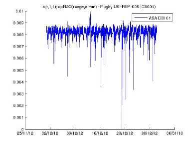
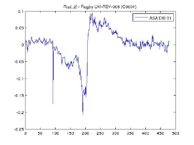
Figure 1: $q_{i}$ vs $i$ (left) and ${\bf v}_{2}$ (right), for a signal from Rugby

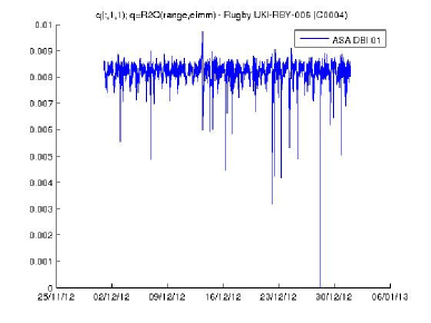
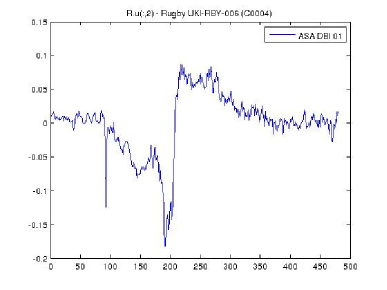
Figure 2: $q_{i}$ vs $i$ (left) and ${\bf v}_{2}$ (right), for a second signal from Rugby

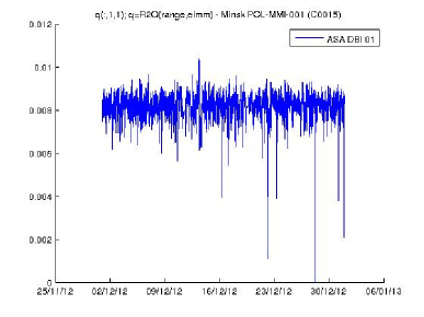
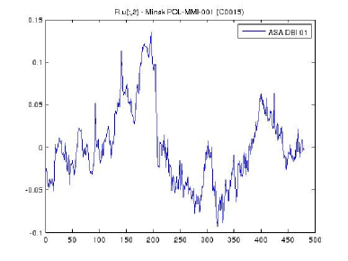
Figure 3: $q_{i}$ vs $i$ (left) and ${\bf v}_{2}$ (right), for a signal from Mińsk Mazowiecki

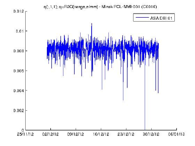
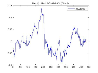
Figure 4: $q_{i}$ vs $i$ (left) and ${\bf v}_{2}$ (right), for a second signal from Mińsk Mazowiecki

4 Quantifying the Similarity between Signatures

The scalar product of two quantum state vectors ${\bf r}$ and ${\bf s}$ with real components is ${\mathbf{r}}^{T}{\mathbf{s}}$ and we can use this to define a measure $D$ of the distance between the states,

$$D({\mathbf{r}},{\mathbf{s}})=\sqrt{1-|{\mathbf{r}}^{T}{\mathbf{s}}|^{2}}$$ (9)

which is zero when the vectors are identical, and is one when they are maximally different (orthogonal). Since the signatures (the ${\bf v}_{2}$ vectors from the SVD) are orthonormal, they have a norm of one, and they are valid quantum state vectors, and we use $D$ to calculate the distance between pairs of them, to quantify their similarity. The distance for carriers from the same antenna turns out to be lower on average than for carriers from different antennas.

5 Performance Evaluation

In order to quantitatively test this approach for identifying signals we developed a statistical model based on histograms of distances between carriers, and applied the model to carrier data that was monitored in Dubai in December 2012, consisting of $53$ carriers from $32$ antennas, which were relayed by the SESAT2 satellite. We initially analysed data from the whole month, and then investigated the performance for shorter periods of time.

5.1 Statistical model and results for data from one month

Figure 5 shows the frequency distributions of distances between pairs of different carriers, from the same antenna, $f_{s}(D)$, and from different antennas, $f_{d}(D)$, using data for each carrier for the whole month. For the 53 carriers there are $\binom{53}{2}=53\times 26=1378$ pairs, 70 of which were from the same antenna, and 1308 of which were from different antennas. It can be seen that the distances between most carriers from the same antenna are much lower than the distances between carriers from different antennas, so fairly good separation can be obtained between carrier pairs from the same antenna and pairs from different antennas.

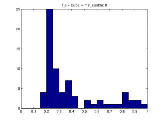
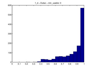
Figure 5: $f_{s}(D)$ (left) and $f_{d}(D)$ (right) - Dubai

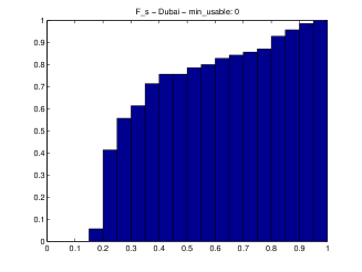
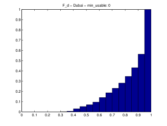
Figure 6: $F_{s}(D)$ (left) and $F_{d}(D)$ (right) - Dubai

The quality of the separation can be characterized using the corresponding relative cumulative frequency distributions, for pairs of carriers from the same antenna, $F_{s}(D)$, and from different antennas, $F_{d}(D)$, shown in figure 6. $F_{s}(D)$ is an estimate of the probability that the distance between a pair of carriers from the same antenna is less than $D$. For example, the value of $F_{s}(0.2)$ is approximately $0.71$. Given the scenario that an interfering carrier is coming from one of a number of known uplink antennas, but we don’t know which one, our approach for identifying the antenna is to calculate the distances from the interferer to all the known carriers from the satellite that is relaying the interferer, and to select those for which the distance $D$ is less than a specified threshold $D_{t}$, and we refer to those carriers as being in the ‘result set’. $F_{s}(D_{t})$ is therefore an estimate of the probability that a given carrier from a satellite is in the result set. Each carrier in the result set that is from the same antenna as the interferer is a positive identification of the source of the interferer, so we refer to these as positives.

5.1.1 Probability of at least one positive

Typically several carriers are transmitted from the same antenna at the same time, so the probability that at least one carrier from the same antenna as the interferer is in the result set is bigger than $F_{s}(D_{t})$, because $F_{s}(D_{t})$ is a probability estimate for a single pair, but on average there is more than one of them. We call this probability $p_{id}$, because it is the probability that at least one carrier has been correctly identified as coming from the same antenna as the interferer. For each known carrier, the probability that it is not in the result set is $1-F_{s}(D_{t})$, so for an antenna with $k$ carriers the probability that none of them are in the result set is $(1-F_{s}(D_{t}))^{k}$. If the number of antennas that have $k$ carriers is $n(k)$, then averaged across antennas, the probability that none of the carriers are in the result set, which we call $\bar{p}_{id}$, is

$$\bar{p}_{id}=\frac{\sum_{k}n(k)(1-F_{s}(D_{t}))^{k}}{\sum_{k}n(k)}.$$ (10)

Now, the sum in the denominator of this equation is equal to the total number of antennas, which we call $N_{a}$ and the probability that at least one carrier in the result set came from the same antenna as the interferer is $1-\bar{p}_{id}$, so

$$p_{id}=1-\frac{1}{N_{a}}\sum_{k}n(k)(1-F_{s}(D_{t}))^{k}.$$ (11)

For the Dubai data in December 2012, 27 of the 32 antennas had only one carrier, and the other five antennas had two, three, six (twice) and nine carriers respectively, so if we choose $D_{t}=0.4$ for our threshold, for which $F_{s}(D_{t})=0.714$, the probability that the antenna we are seeking is in the result set is approximately $p_{id}=0.76$.

5.1.2 Expected number of positives

We call the expected number of positives $n_{i}$, because they are carriers that have been correctly identified as coming from the same antenna as the interferer, and we call the average number of carriers per antenna $n_{s}$, because it is the average number of carriers from the same antenna. Only carriers from the same antenna as the interferer can contribute towards $n_{i}$, and on average there will be $n_{s}$ of them. We can consider the decision as to whether the distance of each of these carriers from that of the interferer is less than $D_{t}$ as being independent trials, so so the probability that a carrier from the same antenna as the interferer is in the result set (the trial is a success) is equal to the number of successes $n_{i}$ divided by the number of trials $n_{s}$, but we know that this probability is given by $F_{s}(D_{t})$, so we have $F_{s}(D_{t})=n_{i}/n_{s}$, which gives an estimate for $n_{i}$ of

$$n_{i}=n_{s}F_{s}(D_{t}).$$ (12)

A more detailed analysis takes into account the distribution of the number of carriers per antenna. We can consider the decisions as to whether the distances between each carrier from the antenna and the interferer are less than $D_{t}$ as being independent trials, so the probability of obtaining $k$ positives from an antenna with $K$ known carriers, which we call $P(k)$, will follow a binomial distribution, and if we let $p=F_{s}(D_{t})$ and $q=1-p$, then

$$P(k)=\binom{K}{k}p^{k}q^{K-k}.$$ (13)

The expected value of $k$ is known to be

$$\bar{k}=\sum_{k}kP(k)=Kp,$$ (14)

and given the distribution $n(K)$, and averaging over $K$, the expected number of positives is

$$n_{i}=\langle\bar{k}\rangle=\frac{p}{N_{a}}\sum_{K}n(K)K=\bar{K}p,$$ (15)

where $\bar{K}=n_{s}$, the average number of carriers from the same antenna, so we obtain the same result as equation 12.

For the Dubai data in December 2012 the value of $n_{s}$ was approximately $1.66$ and $F_{s}(0.4)$ was $0.71$, so $n_{i}$ is therefore approximately $1.2$.

5.1.3 Expected number of false positives

In general the result set will also contain some carriers from antennas other than the one that we are trying to identify, and the number of such false positives, which we call $n_{f}$, can be estimated using $F_{d}(D)$, which is an estimate of the probability that the distance between a pair of carriers from different antennas is less than $D$. A similar argument to the one that led to equation 12 gives

$$n_{f}=n_{d}F_{d}(D_{t}),$$ (16)

where $n_{d}$ is the number of carriers from different antennas to the one that the interferer originated from. We call the number of carriers relayed by the satellite is $N_{s}$, and we know that of these, on average $n_{s}$ of them are from one particular antenna, so the average the number that are from other antennas is

$$n_{d}=N_{s}-n_{s},$$ (17)

so we have

$$n_{f}=(N_{s}-n_{s})F_{d}(D_{t}),$$ (18)

For this example case, 53 carriers were relayed by the satellite, so $N_{s}=53$, and given our example threshold of $D_{t}=0.4$, the value of $F_{d}(0.4)$ is approximately $0.0061$, so we have an estimated number of $n_{f}=n_{d}F_{d}(D_{t})=51.34\times 0.0061$ false positives, which is approximately $0.31$. Note that a slightly higher value of $D_{t}$, say $D_{t}=0.5$, would give a higher expected number of positives, of $n_{i}=1.25$, but also a much higher number of false positives, $n_{f}=2.7$.

Note also that we need not restrict our data to carriers relayed by the same satellite as the interferer, since other satellites may also relay carriers from the antenna that is the source of the interferer, but it was found that for the data at our disposal, including such carriers increased the false positive rate significantly, with little or no increase in the number of positives.

5.1.4 Probability of one or more false positives

For a carrier from an antenna with $K$ carriers there are $N_{s}-K$ possible comparisons with carriers from the other antennas, and if we now let $p=F_{d}(D_{t})$ then the probability of one or more false positives, which we call $p_{f}^{K}$, as it applies to an antenna with $K$ carriers, is

$$p_{f}^{K}=1-(1-p)^{(N_{s}-K)}.$$ (19)

Provided $p$ is small, this approximates to

$$p_{f}^{K}\simeq(N_{s}-K)p,$$ (20)

which happens to also equal the expected number of false positives for that antenna, which we call $n_{f}^{K}$. Provided $N_{s}$ is large and $K$ is small, (20) is not a strong function of K, and with this assumption

$$p_{f}^{K}=n_{f}^{K}\simeq N_{s}p\simeq\langle p_{f}^{K}\rangle=\langle n_{f}^{K}\rangle,$$ (21)

and this would be the expected result averaged over all the antennas, which we call $p_{f}=\langle p_{f}^{K}\rangle$, and we have

$$p_{f}\simeq N_{s}p=N_{s}F_{d}(D_{t}),$$ (22)

For the Dubai data in December 2012 the probability of a false positive is therefore approximately $p_{f}=0.32$.

5.2 Results for data from two days

So far we have presented data from a period of one month, but we also tried analysing data from shorter periods of time, and found that results with $n_{i}>n_{f}$ could be obtained for periods right down to two days, which was the minimum amount of data necessary for the algorithm to work in its original form. However, we found that the results were better for some two-day periods than for others. This can be seen from figures 7 and 8, which show the frequency distributions of distances between pairs of carriers from the same antenna, $f_{s}(D)$, and from different antennas, $f_{d}(D)$, for data monitored by Dubai for two different two-day periods in December 2012. Note that the number of counts in figure 7 (left) is roughly twice that of figure 8 (left), which is because not all carriers were present for the whole month, and for each period, only carriers were considered that were present for the whole of the period. The data in figure 7 is for pairs taken from 68 carriers, and in figure 8 it is from 54 carriers. The average number of carriers per antenna was also higher for the data in figure 7, which further boosted the number of pairs.

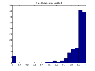
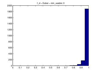
Figure 7: $f_{s}(D)$ (left) and $f_{d}(D)$ (right) - Dubai, 1-2 Dec. 2012

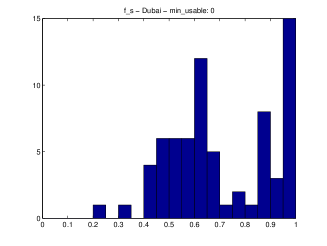
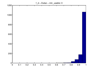
Figure 8: $f_{s}(D)$ (left) and $f_{d}(D)$ (right) - Dubai, 15-16 Dec. 2012

The best separation is shown by the data from 15-16 December 2012, for which a choice of $D_{t}=0.7$ gives $p_{id}=0.64$, $n_{i}=0.97$, $n_{f}=0.19$, and $p_{f}=0.20$.

5.3 Results for data from less than two days

The algorithm was designed to require a minimum of two days of data (two periods of 24 hours each), as it compared one day with the next, in order to remove the 24 hour variation that is present in all carriers, and all of the results presented in the previous sections used that version of the algorithm. We then decided to investigate whether the algorithm could still identify characteristic features of carriers if it was modified to use periods of less than 24 hours, which would mean that the 24 hour variation was not removed. The modified algorithm still compares data from equal-length periods, and there must be at least two of them, but they can be of arbitrary length, and in particular, less than 24 hours.

Figure 9 shows the frequency distributions of distances between pairs of carriers from the same antenna, $f_{s}(D)$, and from different antennas, $f_{d}(D)$, for one day’s data, monitored at Dubai for December 15th 2012, split into two 12 hour periods. It can be seen that there is some separation between carrier pairs from the same antenna and pairs from different antennas, and choosing $D_{t}=0.85$ gives $p_{id}=0.62$, $n_{i}=0.93$, $n_{f}=0.92$, and $p_{f}=0.95$.

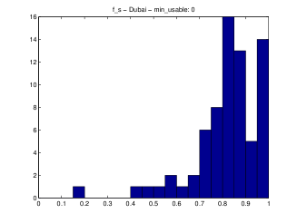
Figure 9: $f_{s}(D)$ (left) and $f_{d}(D)$ (right) - Dubai, 15 Dec. 2012

Figure 10 shows the frequency distributions of distances between pairs of carriers from the same antenna, $f_{s}(D)$, and from different antennas, $f_{d}(D)$, for half a day’s data, monitored at Dubai for the first 12 hours of December 15th 2012, split into two 6 hour periods. Again it can be seen that there is some separation between carrier pairs from the same antenna and pairs from different antennas, and choosing $D_{t}=0.85$ gives $p_{id}=0.33$, $n_{i}=0.33$, $n_{f}=0.69$, and $p_{f}=0.71$.

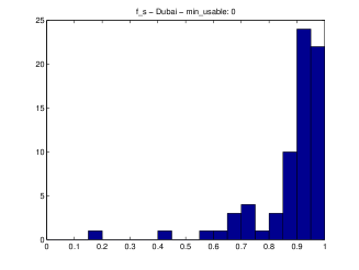
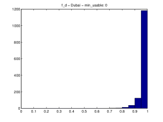
Figure 10: $f_{s}(D)$ (left) and $f_{d}(D)$ (right) - 0:00–12:00, Dubai, 15 Dec. 2012

It is encouraging that the algorithm works at all for less than one day’s data, and although the results presented here show that it works less well for shorter periods, this is based on a fixed sampling rate of $\mathrm{EIRP}$ values, meaning that the shorter periods contain less data. As long as the signal contains enough structure, a higher sampling rate should give better results.

6 Conclusion

We have described a method for identifying the source of a satellite interferer using a single satellite, which relies on the variation with time of the strength of carrier signals measured at the downlink station. The method uses a quantum-inspired algorithm to compute a signature for each carrier, and a distance between the signature for an interfering carrier and the signatures of all known carriers being relayed by the same satellite. As a proof of concept we have presented a simple statistical model to estimate the probability of successful identification of the source of an interferer, the expected number of carriers correctly identified to have originated from the interfering transmitter, the expected number of false positives, and the probability of one or more false positives, and we have used the model to evaluate the performance of the technique using measured data for a sample of 53 carriers relayed by one satellite. We presented results using data from one month, and also for two days and less. In its original form the algorithm was designed to work with a minimum of two days’ of data, and we found that the results were better for some two-day periods than others, but that in some cases successful identification was possible. We also modified the algorithm to operate on less than two days’ of data, and we found that the results were less good, but that positive identification was still possible in some cases. However, the results were based on a fixed sampling rate, meaning that the shorter periods contained less data, and a higher sampling rate should give better results.

References

- [1] Martin Coleman. Jamming overview. ITU Workshop on the efficient use of the spectrum/orbit resource, Limassol, Cyprus, April 2014.
- [2] Ibrahim Öz. Harmful interference: regional security consequences. UNIDIR regional seminar: Building confidence for Eurasian space activities through norms of behaviour, Astana, Kazakhstan, October 2013.
- [3] Paul C. Chestnut. Emitter location accuracy using TDOA and differential Doppler. IEEE Transactions on Aerospace and Electronic Systems, AES-18(2):214–218, March 1982.
- [4] William W. Smith and Paul G. Steffes. Time delay techniques for satellite interference location system. IEEE Transactions on Aerospace and Electronic Systems, 25(2):224–231, March 1989.
- [5] John Effland, John M. Gipson, David B. Shaffer, and John C. Webber. Method and system for locating an unknown transmitter. US patent US5008679 (A), April 1991.
- [6] D. P. Haworth, N. G. Smith, R. Bardelli, and T. Clement. Interference localization for EUTELSAT satellites-the first European transmitter location system. International Journal of Satellite Communications and Networking, 15(4):155–183, 1997.
- [7] Howard Grant, Eric Salt, and David Dodds. Geolocation of communications satellite interference. In 2013 26th Annual IEEE Canadian Conference on Electrical and Computer Engineering (CCECE), 2013.
- [8] Ramoni O. Adeogun. A robust MUSIC based scheme for interference location in satellite systems with multibeam antennas. International Journal of Computer Applications, 82(12):1–6, November 2013.
- [9] Brian C. Fredrick. Geolocation of source interference from a single satellite with multiple antennas. Master’s thesis, Naval Postgraduate School, Monterey, California, March 2014.
- [10] Dominic Ho, Jeffrey Chu, and Michael Downey. Determining transmit location of an emitter using a single geostationary satellite. US patent US8462044 (B1), June 2013.
- [11] Ashkan Kalantari, Sina Maleki, Symeon Chatzinotas, and Björn Ottersten. Frequency of arrival-based interference localization using a single satellite. In 2016 8th Advanced Satellite Multimedia Systems Conference and the 14th Signal Processing for Space Communications Workshop (ASMS/SPSC), 2016.
- [12] Michael Nölle. Verfahren zur Identifikation von Störsendern. Austrian patent AT515001 (B1), August 2015.
- [13] Michael Nölle. Method for identifying interfering transmitters from a plurality of known satellite transmitters. International patent application WO2015062810 (A1), May 2015.
- [14] Michael Nölle. Method for identifying interfering transmitters from a plurality of known satellite transmitters. US patent application US2016254856 (A1), September 2016.
- [15] Michael Nölle. Method for identifying interfering transmitters from a plurality of known satellite transmitters. European patent application EP3063879 (A1), September 2016.
- [16] Michael Nölle, Bernhard Ömer, and Martin Suda. Quantum information algorithms – new solutions for known problems. e & i Elektrotechnik und Informationstechnik, 124(5):154–157, 2007.
- [17] Michael Nölle and Martin Suda. Conjugate variables as a resource in signal and image processing, August 2011.
- [18] Michael Nölle, Martin Suda, and Winfried Boxleitner. H2SI - A new perceptual colour space. In 18th International Conference on Digital Signal Processing, DSP 2013, Fira, Santorini, Greece, July 1-3, 2013, pages 1–6, 2013.
- [19] Yu. I. Bogdanov, N. A. Bogdanova, V. F. Lukichev, D. V. Fastovets, and A. Yu. Chernyavskii. Schmidt decomposition and analysis of statistical correlations. Russian Microelectronics, 45(5):314–323, 2016.
- [20] Michael A. Nielsen and Isaac L. Chuang. Quantum Computation and Quantum Information: 10th Anniversary Edition. Cambridge University Press, New York, NY, USA, 10th edition, 2011.
- [21] I.T. Jolliffe. Principal Component Analysis. Springer Series in Statistics. Springer, 2002.
- [22] M. A. Turk and A. P. Pentland. Face recognition using eigenfaces. In Proceedings. 1991 IEEE Computer Society Conference on Computer Vision and Pattern Recognition, pages 586–591, Jun 1991.