A possible partner state of the $Y(2175)$

Abstract

We study the $Y(2175)$ using the method of QCD sum rules. There are two independent $ss\bar{s}\bar{s}$ interpolating currents with $J^{PC}=1^{--}$, and we calculate both their diagonal and off-diagonal correlation functions. We obtain two new currents which do not strongly correlate to each other, so they may couple to two different physical states: one of them couples to the $Y(2175)$, while the other may couple to another state whose mass is about $71^{+172}_{-~{}48}$ MeV larger. Evidences of the latter state can be found in the BaBar Aubert:2007ur , BESII Ablikim:2007ab , Belle Shen:2009zze , and BESIII Ablikim:2014pfc experiments.

I Introduction

In recent years there have been lots of exotic hadrons observed in hadron experiments pdg , which can not be explained in the traditional quark model and are of particular importance to understand the low energy behaviours of Quantum Chromodynamics (QCD) Chen:2016qju ; Klempt:2007cp ; Lebed:2016hpi ; Esposito:2016noz ; Guo:2017jvc ; Ali:2017jda ; Olsen:2017bmm . Most of them contain heavy quarks, such as the charmonium-like $XYZ$ states, while there are not so many exotic hadrons in the light sector only containing light $u/d/s$ quarks. The $Y(2175)$ is one of them, which is often taken as the strange analogue of the $Y(4220)$ Aubert:2005rm ; Ablikim:2016qzw .

The $Y(2175)$ was first observed in 2006 by the BaBar Collaboration in the $\phi f_{0}(980)$ invariant mass spectrum Aubert:2006bu ; Aubert:2007ur ; Aubert:2007ym ; Lees:2011zi , and later confirmed in the BESII Ablikim:2007ab , Belle Shen:2009zze , and BESIII Ablikim:2014pfc ; Ablikim:2017auj experiments. Its mass and width were measured to be $M=2188\pm 10$ MeV and $\Gamma=83\pm 12$ MeV respectively, and its spin-parity quantum number is $J^{PC}=1^{--}$ pdg . We list some of these experiments in Fig. 1, including:

1. Fig. 1(a): the BaBar experiment Aubert:2006bu discovering the $Y(2175)$ in the $e^{+}e^{-}\to\phi f_{0}(980)$ cross section in 2006.

2. Fig. 1(b): the BaBar experiment Aubert:2007ur in 2007.

3. Fig. 1(c): the Belle experiment Shen:2009zze in 2009.

4. Fig. 1(d): a combined fit to the BaBar Aubert:2006bu ; Aubert:2007ur and Belle Shen:2009zze measurements of the $e^{+}e^{-}\to\phi f_{0}(980)$ cross sections, performed by Shen and Yuan in Ref. Shen:2009mr .

5. Fig. 1(e): the BESII experiment Ablikim:2007ab in 2007.

6. Fig. 1(f): the BESIII experiment Ablikim:2014pfc in 2014.

Besides the $Y(2175)$, there might be another structure in the $\phi f_{0}(980)$ invariant mass spectrum at around 2.4 GeV, whose evidences can be found in the BaBar Aubert:2007ur (Fig. 1(b) around 2.4 GeV), Belle Shen:2009zze (Fig. 1(c) around 2.40 GeV), BESII Ablikim:2007ab (Fig. 1(e) around 2.46 GeV), and BESIII Ablikim:2014pfc (Fig. 1(f) around 2.35 GeV) experiments. The BaBar experiment Aubert:2007ur determined its mass and width to be $2.47\pm 0.07$ GeV and $77\pm 65$ MeV, respectively. Shen and Yuan Shen:2009mr also used the BaBar Aubert:2006bu ; Aubert:2007ur and Belle Shen:2009zze data to fit its mass and width to be $2436\pm 34$ MeV and $99\pm 105$ MeV, respectively. However, its statistical significance is smaller than $3.0\sigma$. In this paper we shall study this structure as well as the $Y(2175)$ simultaneously using the method of QCD sum rules.

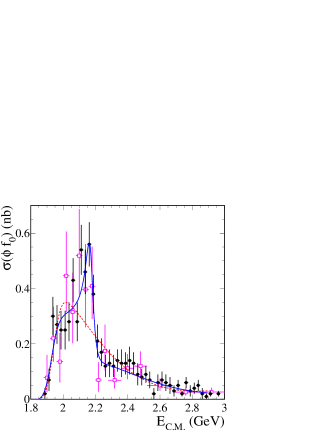
(a) The $e^{+}e^{-}\to\phi f_{0}(980)$ cross section. Taken from BaBar Aubert:2006bu .

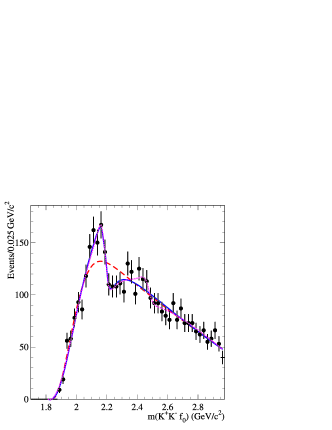
(b) The $K^{+}K^{-}\pi^{+}\pi^{-}$ invariant mass distribution in the $K^{+}K^{-}f_{0}(980)$ threshold region. The fits are done by including no (dashed), one (solid) and two (dotted) resonances. Taken from BaBar Aubert:2007ur .

(c) The $e^{+}e^{-}\to\phi\pi^{+}\pi^{-}$ cross section with two incoherent Briet-Wigner functions, the $\phi(1680)$ and the $Y(2175)$. Taken from Belle Shen:2009zze .

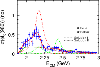
(d) Fits to the BaBar Aubert:2006bu ; Aubert:2007ur and Belle Shen:2009zze measurements of the $e^{+}e^{-}\to\phi f_{0}(980)$ cross sections with two coherent Briet-Wigner functions, performed by Shen and Yuan and taken from Ref. Shen:2009mr .

(e) The $\phi f_{0}(980)$ invariant mass spectrum. Taken from BESII Ablikim:2007ab .

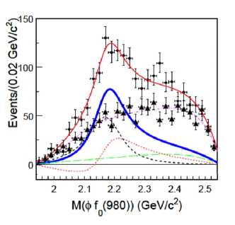
(f) The $\phi f_{0}(980)$ invariant mass spectrum. Taken from BESIII Ablikim:2014pfc .

Figure 1: The BaBar Aubert:2006bu ; Aubert:2007ur , Belle Shen:2009zze , BESII Ablikim:2007ab , and BESIII Ablikim:2014pfc experiments observing the $Y(2175)$ as well as the fit performed in Ref. Shen:2009mr .

Since its discovery, the $Y(2175)$ has attracted much attention from the hadron physics community, and many theoretical methods and models were applied to study it. By using both the chiral unitary model Napsuciale:2007wp ; GomezAvila:2007ru and the Faddeev equations MartinezTorres:2008gy , the authors interpreted the $Y(2175)$ as a dynamically generated state in the $\phi K\bar{K}$ and $\phi\pi\pi$ systems, and more states were predicted in the $\phi\pi^{0}\eta$ VaqueraAraujo:2009jq and $NK\bar{K}$ MartinezTorres:2009cw ; Xie:2010ig systems. By using similar approaches, the $Y(2175)$ was interpreted as a dynamically generated resonance by the self-interactions between the $\phi$ and $f_{0}(980)$ resonances AlvarezRuso:2009xn , while the resonance spectrum expansion formalism by including the $f_{0}(980)$ as a resonance in the coupled $\pi\pi$-$KK$ system is also able to generate the $Y(2175)$ in the $\phi f_{0}(980)$ channel Coito:2009na .

Besides the dynamically generated resonance, there are many other interpretations to explain this structure. In Ref. Ding:2007pc the authors interpreted the $Y(2175)$ as a $2^{3}D_{1}$ $s\bar{s}$ meson, and calculated its decay modes using both the ${}^{3}P_{0}$ model and the flux-tube model. In Ref. Abud:2009rk the authors used a constituent quark model to interpret the $Y(2175)$ as a hidden-strangeness baryon-antibaryon state ($qqs\bar{q}\bar{q}\bar{s}$) strongly coupling to the $\Lambda\bar{\Lambda}$ channel. Later in Ref. Zhao:2013ffn the authors applied the one-boson-exchange model to interpret the $Y(2175)$ and $\eta(2225)$ as the bound states of $\Lambda\bar{\Lambda}(^{3}S_{1})$ and $\Lambda\bar{\Lambda}(^{1}S_{0})$, respectively. In Ref. Ding:2006ya the authors interpreted the $Y(2175)$ as a strangeonium hybrid state and used the flux-tube model to study its decay properties. However, this interpretation is not supported by the non-perturbative lattice QCD calculations Dudek:2011bn . Productions of the $Y(2175)$ were studied in Refs. Bystritskiy:2007wq ; Ali:2011qi by using the Nambu-Jona-Lasinio model and the Drell-Yan mechanism, while its decay properties were studied in Refs. Chen:2011cj ; Wang:2012wa via the initial single pion emission mechanism.

The method of QCD sum rules was also applied to study the $Y(2175)$ Wang:2006ri ; Chen:2008ej , which method has been widely and successfully used to study hadron properties Shifman:1978bx ; Reinders:1984sr . When using this method to investigate a physical state, one needs to construct the relevant interpolating current, but we still do not fully understand their relations: a) the interpolating current sees only the quantum numbers of the physical state, so it can also couple to some other physical states as well as the relevant threshold; b) one can sometimes construct more than one interpolating currents, all of which can couple to the same physical state. Some previous studies tell us that:

1. In Ref. Chen:2015kpa we systematically studied the $P$-wave singly heavy baryons. Theoretically, we find that they have rich internal structures, and there can be as many as three excited $\Omega_{c}$ states of $J^{P}=1/2^{-}$, three of $J^{P}=3/2^{-}$, and one of $J^{P}=5/2^{-}$. For each state we can construct one interpolating current having the same internal structure. The numbers of excited $\Lambda_{c}/\Xi_{c}/\Sigma_{c}/\Xi_{c}^{\prime}$ states/currents are the same.

   We do not know which of them exist in nature, but we do know that, experimentally, the $P$-wave charmed baryons also have rich structures Chen:2016spr , for example, the LHCb experiment Aaij:2017nav observed as many as five excited $\Omega_{c}$ states at the same time, all of which can be $P$-wave charmed baryons.

2. In Ref. Chen:2010ze the mass spectra of vector and axial-vector hidden-charm tetraquark states were systematically investigated. There can be as many as eight $qc\bar{q}\bar{c}$ ($q=u/d$) interpolating currents of $J^{PC}=1^{--}$. Comparably, there have been many vector charmonium-like states observed in hadron experiments pdg , including the $Y(4008)$ Yuan:2007sj , $Y(4220)$ Aubert:2005rm , $Y(4320)$ Ablikim:2016qzw , $Y(4360)$ Aubert:2007zz , $Y(4630)$ Pakhlova:2008vn , and $Y(4660)$ Wang:2007ea , etc.

3. In Ref. Chen:2016otp we systematically studied hidden-charm pentaquark states having spin $J={1\over 2}/{3\over 2}/{5\over 2}$. We constructed hundreds of hidden-charm pentaquark interpolating currents, suggesting that their internal structures are rather complicated. However, the only observed hidden-charm pentaquark states so far are the $P_{c}(4380)$ and $P_{c}(4450)$ Aaij:2015tga , and it is unbelievable that there exist hundreds of hidden-charm pentaquark states in nature.

Hence, the internal structures of (exotic) hadrons are complicated. For each internal structure we can construct the relevant interpolating current, and their relations are also complicated. Especially, there can be many interpolating currents when studying exotic hadrons, which makes them not easy to handle.

To clarify this problem, a good subject is to study the $Y(2175)$ of $J^{PC}=1^{--}$. The relevant $ss\bar{s}\bar{s}$ interpolating currents have been systematically constructed in Ref. Chen:2008ej , and there are only two independent ones. We have separately used them to perform QCD sum rule analyses, both of which can be used to explain the $Y(2175)$. However, in Ref. Chen:2008ej we only calculated the diagonal terms of these two currents, and in this work we shall further calculate their off-diagonal term to study their correlation. This can significantly improve our understanding on the relations between interpolating currents and physical states.

Another advantage to study the $Y(2175)$ is that, experimentally, there might be another structure in the $\phi f_{0}(980)$ invariant mass spectrum at around 2.4 GeV, as we have discussed before. It is quite interesting to study the relations between the two independent $ss\bar{s}\bar{s}$ currents with $J^{PC}=1^{--}$ and the two possible structures in the $\phi f_{0}(980)$ invariant mass spectrum, both theoretically and experimentally, and both coherently and incoherently. Note that there are many charmonium-like $Y$ states of $J^{PC}=1^{--}$, so it is natural to think that there can be more than one $Y$ states in the light sector.

This paper is organized as follows. In Sec. II, we list the two independent $ss\bar{s}\bar{s}$ interpolating currents with $J^{PC}=1^{--}$, and discuss how to diagonalize them. In Sec. III, we use two diquark-antidiquark $(ss)(\bar{s}\bar{s})$ interpolating currents to perform QCD sum rule analyses, and obtain two new currents which do not strongly correlate to each other. In Sec. IV, we use these two new currents to calculate mass spectra, and Sec. V is a summary.

II Interpolating currents and their relations to possible physical states

The interpolating currents having the quark content $ss\bar{s}\bar{s}$ and with the quantum number $J^{PC}=1^{--}$ have been systematically constructed in Ref. Chen:2008ej . We briefly summarize the results here and discuss their relations to possible physical states.

1. There are two non-vanishing diquark-antidiquark $(ss)(\bar{s}\bar{s})$ interpolating currents with $J^{PC}=1^{--}$:

   $$\eta_{1\mu}=$$ (1)

   $$~{}~{}~{}(s_{a}^{T}C\gamma_{5}s_{b})(\bar{s}_{a}\gamma_{\mu}\gamma_{5}C\bar{s}_{b}^{T})-(s_{a}^{T}C\gamma_{\mu}\gamma_{5}s_{b})(\bar{s}_{a}\gamma_{5}C\bar{s}_{b}^{T})\,,$$

   $$\eta_{2\mu}=$$ (2)

   $$~{}~{}~{}(s_{a}^{T}C\gamma^{\nu}s_{b})(\bar{s}_{a}\sigma_{\mu\nu}C\bar{s}_{b}^{T})-(s_{a}^{T}C\sigma_{\mu\nu}s_{b})(\bar{s}_{a}\gamma^{\nu}C\bar{s}_{b}^{T})\,,$$

   where $a$ and $b$ are color indices, $C=i\gamma_{2}\gamma_{0}$ is the charge conjugation operator, and the superscript $T$ represents the transpose of Dirac indices. These two currents are independent of each other.

2. There are four non-vanishing meson-meson $(\bar{s}s)(\bar{s}s)$ interpolating currents with $J^{PC}=1^{--}$:

   $$\eta_{3\mu} = (\bar{s}_{a}s_{a})(\bar{s}_{b}\gamma_{\mu}s_{b})\,,$$ (3)

   $$\eta_{4\mu} = (\bar{s}_{a}\gamma^{\nu}\gamma_{5}s_{a})(\bar{s}_{b}\sigma_{\mu\nu}\gamma_{5}s_{b})\,,$$ (4)

   $$\eta_{5\mu} = {\lambda_{ab}}{\lambda_{cd}}(\bar{s}_{a}s_{b})(\bar{s}_{c}\gamma_{\mu}s_{d})\,,$$ (5)

   $$\eta_{6\mu} = {\lambda_{ab}}{\lambda_{cd}}(\bar{s}_{a}\gamma^{\nu}\gamma_{5}s_{b})(\bar{s}_{c}\sigma_{\mu\nu}\gamma_{5}s_{d})\,.$$ (6)

   However, only two of them are independent.

3. When using local currents, we can verify the following relations between the above $(ss)(\bar{s}\bar{s})$ and $(\bar{s}s)(\bar{s}s)$ currents through the Fierz transformation:

   $$\eta_{1\mu}(x) = -\eta_{3\mu}(x)+i\eta_{4\mu}(x)\,,$$ (7)

   $$\eta_{2\mu}(x) = 3i\eta_{3\mu}(x)-\eta_{4\mu}(x)\,.$$

In Ref. Chen:2008ej we have separately used $\eta_{1\mu}$ and $\eta_{2\mu}$ to perform QCD sum rule analyses, i.e., we have calculated the diagonal terms:

$$\langle 0|T\eta_{1\mu}(x){\eta_{1\nu}^{\dagger}}(0)|0\rangle~{}~{}~{}{\rm and}~{}~{}~{}\langle 0|T\eta_{2\mu}(x){\eta_{2\nu}^{\dagger}}(0)|0\rangle\,.$$ (8)

However, although $\eta_{1\mu}$ and $\eta_{2\mu}$ are independent of each other, they can be correlated to each other, i.e., the off-diagonal term can be non-zero:

$$\langle 0|T\eta_{1\mu}(x){\eta_{2\nu}^{\dagger}}(0)|0\rangle\neq 0\,,$$ (9)

suggesting that $\eta_{1\mu}$ and $\eta_{2\mu}$ may couple to the same physical state. In this paper we shall evaluate this off-diagonal term in order to find two non-correlated currents:

$$J_{1\mu} = \cos\theta~{}\eta_{1\mu}+\sin\theta~{}i~{}\eta_{2\mu}\,,$$ (10)

$$J_{2\mu} = \sin\theta~{}\eta_{1\mu}+\cos\theta~{}i~{}\eta_{2\mu}\,,$$

satisfying

$$\langle 0|TJ_{1\mu}(x){J_{2\nu}^{\dagger}}(0)|0\rangle=0\,,$$ (11)

$$~{}~{}~{}~{}~{}~{}~{}~{}~{}~{}~{}~{}~{}~{}~{}~{}{\rm or}~{}~{}~{}\left\{\begin{array}[]{c}\ll\langle 0|TJ_{1\mu}(x){J_{1\nu}^{\dagger}}(0)|0\rangle\\ \ll\langle 0|TJ_{2\mu}(x){J_{2\nu}^{\dagger}}(0)|0\rangle\end{array}\right.\,.$$ (14)

Then we shall use $J_{1\mu}$ and $J_{2\mu}$ to perform QCD sum rule analyses. Due to the above Eq. (11), $J_{1\mu}$ and $J_{2\mu}$ should not strongly couple to the same physical state, so we assume

$$\langle 0|J_{1\mu}|Y_{1}\rangle = f_{1}~{}\epsilon_{\mu}\,,$$ (15)

$$\langle 0|J_{2\mu}|Y_{2}\rangle = f_{2}~{}\epsilon_{\mu}\,,$$ (16)

where $Y_{1}$ and $Y_{2}$ are two different states with $J^{PC}=1^{--}$, $f_{1}$ and $f_{2}$ are decay constants, and $\epsilon_{\mu}$ is the polarization vector. Especially, we shall evaluate the mass splitting between these two states/currents.

III QCD sum rule Analysis

The method of QCD sum rules is a powerful and successful non-perturbative method Shifman:1978bx ; Reinders:1984sr . In this method, we calculate the two-point correlation function

$$\Pi_{\mu\nu}(q^{2})\,\equiv\,i\int d^{4}xe^{iqx}\langle 0|T\eta_{\mu}(x){\eta_{\nu}^{\dagger}}(0)|0\rangle\,,$$ (17)

at both the hadron and quark-gluon levels.

At the hadron level we simplify its Lorentz structure to be:

$$\Pi_{\mu\nu}(q^{2})=({q_{\mu}q_{\nu}\over q^{2}}-g_{\mu\nu})\Pi(q^{2})+{q_{\mu}q_{\nu}\over q^{2}}\Pi^{(0)}(q^{2})\,,$$ (18)

and express $\Pi(q^{2})$ in the form of the dispersion relation:

$$\Pi(q^{2})=\int^{\infty}_{16m_{s}^{2}}\frac{\rho(s)}{s-q^{2}-i\varepsilon}ds\,.$$ (19)

Here $\rho(s)$ is the spectral density, for which we adopt a parametrization of one pole dominance for the ground state $Y$ and a continuum contribution:

$$\rho(s) \equiv \sum_{n}\delta(s-M^{2}_{n})\langle 0|\eta|n\rangle\langle n|{\eta^{\dagger}}|0\rangle\$$ (20)

$$= f^{2}_{Y}\delta(s-M^{2}_{Y})+\rm{continuum}\,.$$

At the quark-gluon level, we insert $J_{1\mu}$ and $J_{2\mu}$ into Eq. (17), and calculate the correlation function using the method of operator product expansion (OPE). After performing the Borel transformation at both the hadron and quark-gluon levels, we obtain

$$\Pi^{(all)}(M_{B}^{2})\equiv\mathcal{B}_{M_{B}^{2}}\Pi(p^{2})=\int^{\infty}_{16m_{s}^{2}}e^{-s/M_{B}^{2}}\rho(s)ds\,.$$ (21)

After approximating the continuum using the spectral density of OPE above a threshold value $s_{0}$, we obtain the sum rule equation

$$\Pi(M_{B}^{2})\equiv f^{2}_{Y}e^{-M_{Y}^{2}/M_{B}^{2}}=\int^{s_{0}}_{16m_{s}^{2}}e^{-s/M_{B}^{2}}\rho(s)ds\,.$$ (22)

We can use this equation to calculate $M_{Y}$ through

$$M^{2}_{Y}=\frac{\frac{\partial}{\partial(-1/M_{B}^{2})}\Pi(M_{B}^{2})}{\Pi(M_{B}^{2})}=\frac{\int^{s_{0}}_{16m_{s}^{2}}e^{-s/M_{B}^{2}}s\rho(s)ds}{\int^{s_{0}}_{16m_{s}^{2}}e^{-s/M_{B}^{2}}\rho(s)ds}\,.$$ (23)

The sum rules for the currents $\eta_{1\mu}$ and $\eta_{2\mu}$ have been separately calculated and given in Eqs. (13) and (14) of Ref. Chen:2008ej . In this paper we revise these calculations by adding the diagram shown in Fig. 2. We write them as $\Pi_{\eta_{1}\eta_{1}}(q^{2})$ and $\Pi_{\eta_{2}\eta_{2}}(q^{2})$ in the present study, which are transformed to be $\Pi_{\eta_{1}\eta_{1}}(M_{B}^{2})$ and $\Pi_{\eta_{2}\eta_{2}}(M_{B}^{2})$ after the Borel transformation. The results are shown in Eqs. (III) and (III), which do not change significantly compared to Ref. Chen:2008ej .

Figure 2: Feynman diagram related to the quark-gluon mixed condensate $\langle g_{s}\bar{s}\sigma Gs\rangle$.

In Eqs. (III) and (III) we have calculated the OPE up to twelve dimension, including the strange quark mass, the perturbative term, the quark condensate $\langle\bar{s}s\rangle$, the gluon condensate $\langle g_{s}^{2}GG\rangle$, the quark-gluon mixed condensate $\langle g_{s}\bar{s}\sigma Gs\rangle$, and their combinations $\langle\bar{s}s\rangle^{2}$, $\langle\bar{s}s\rangle^{3}$, $\langle\bar{s}s\rangle^{4}$, $\langle g_{s}\bar{s}\sigma Gs\rangle^{2}$, $\langle\bar{s}s\rangle\langle g_{s}\bar{s}\sigma Gs\rangle$, $\langle\bar{s}s\rangle^{2}\langle g_{s}\bar{s}\sigma Gs\rangle$, $\langle g_{s}^{2}GG\rangle\langle\bar{s}s\rangle$, $\langle g_{s}^{2}GG\rangle\langle\bar{s}s\rangle^{2}$, $\langle g_{s}^{2}GG\rangle\langle g_{s}\bar{s}\sigma Gs\rangle$, and $\langle g_{s}^{2}GG\rangle\langle\bar{s}s\rangle\langle g_{s}\bar{s}\sigma Gs\rangle$. These parameters take the following values Yang:1993bp ; Narison:2002pw ; Gimenez:2005nt ; Jamin:2002ev ; Ioffe:2002be ; Ovchinnikov:1988gk ; Ellis:1996xc ; pdg :

$$\langle\bar{q}q\rangle=-(0.24\pm 0.01\mbox{ GeV})^{3}\,,$$

$$\langle\bar{s}s\rangle=-(0.8\pm 0.1)\times(0.240\mbox{ GeV})^{3}\,,$$

$$\langle g_{s}^{2}GG\rangle=(0.48\pm 0.14)\mbox{ GeV}^{4}\,,$$

$$\langle g_{s}\bar{q}\sigma Gq\rangle=-M_{0}^{2}\times\langle\bar{q}q\rangle\,,$$ (24)

$$M_{0}^{2}=(0.8\pm 0.2)\mbox{ GeV}^{2}\,,$$

$$m_{s}(2\mbox{ GeV})=96^{+8}_{-4}\mbox{ MeV}\,,$$

$$\alpha_{s}(1.7\mbox{GeV})=0.328\pm 0.03\pm 0.025\,.$$

Beside the diagonal terms $\Pi_{\eta_{1}\eta_{1}}(q^{2})$ and $\Pi_{\eta_{2}\eta_{2}}(q^{2})$, in the present study we also calculate the sum rules for the off-diagonal term:

$$\Pi_{\mu\nu}^{\eta_{1}\eta_{2}}(q^{2}) = i\int d^{4}xe^{iqx}\langle 0|T\eta_{1\mu}(x){\eta_{2\nu}^{\dagger}}(0)|0\rangle$$

$$= ({q_{\mu}q_{\nu}\over q^{2}}-g_{\mu\nu})\Pi_{\eta_{1}\eta_{2}}(q^{2})+{q_{\mu}q_{\nu}\over q^{2}}\Pi^{(0)}_{\eta_{1}\eta_{2}}(q^{2})\,.$$

After performing the Borel transformation to $\Pi_{\eta_{1}\eta_{2}}(q^{2})$, we obtain $\Pi_{\eta_{1}\eta_{2}}(M_{B}^{2})$ as shown in Eq. (III).

$$\Pi_{\eta_{1}\eta_{1}} = \int^{s_{0}}_{16m_{s}^{2}}\Bigg{[}{s^{4}\over 18432\pi^{6}}-{m_{s}^{2}s^{3}\over 256\pi^{6}}+\Big{(}-{\langle g^{2}GG\rangle\over 18432\pi^{6}}+{m_{s}\langle\bar{s}s\rangle\over 48\pi^{4}}\Big{)}s^{2}$$

$$+\Big{(}{\langle\bar{s}s\rangle^{2}\over 18\pi^{2}}-{m_{s}\langle g\bar{s}\sigma Gs\rangle\over 32\pi^{4}}+{17m_{s}^{2}\langle g^{2}GG\rangle\over 9216\pi^{6}}\Big{)}s+\Big{(}{\langle\bar{s}s\rangle\langle g\bar{s}\sigma Gs\rangle\over 8\pi^{2}}-{m_{s}\langle g^{2}GG\rangle\langle\bar{s}s\rangle\over 128\pi^{4}}-{29m_{s}^{2}\langle\bar{s}s\rangle^{2}\over 12\pi^{2}}\Big{)}\Bigg{]}e^{-s/M_{B}^{2}}ds$$

$$+\Big{(}{5\langle g^{2}GG\rangle\langle\bar{s}s\rangle^{2}\over 864\pi^{2}}+{\langle g\bar{s}\sigma Gs\rangle^{2}\over 24\pi^{2}}+{20m_{s}\langle\bar{s}s\rangle^{3}\over 9}-{5m_{s}\langle g^{2}GG\rangle\langle g\bar{s}\sigma Gs\rangle\over 2304\pi^{4}}-{13m_{s}^{2}\langle\bar{s}s\rangle\langle g\bar{s}\sigma Gs\rangle\over 8\pi^{2}}\Big{)}$$

$$+{1\over M_{B}^{2}}\Big{(}-{32g^{2}\langle\bar{s}s\rangle^{4}\over 81}-{\langle g^{2}GG\rangle\langle\bar{s}s\rangle\langle g\bar{s}\sigma Gs\rangle\over 576\pi^{2}}-{19m_{s}\langle\bar{s}s\rangle^{2}\langle g\bar{s}\sigma Gs\rangle\over 18}+{m_{s}^{2}\langle g^{2}GG\rangle\langle\bar{s}s\rangle^{2}\over 576\pi^{2}}+{m_{s}^{2}\langle g\bar{s}\sigma Gs\rangle^{2}\over 16\pi^{2}}\Big{)}\,,$$

$$\Pi_{\eta_{2}\eta_{2}} = \int^{s_{0}}_{16m_{s}^{2}}\Bigg{[}{s^{4}\over 12288\pi^{6}}-{3m_{s}^{2}s^{3}\over 512\pi^{6}}+\Big{(}{\langle g^{2}GG\rangle\over 18432\pi^{6}}+{m_{s}\langle\bar{s}s\rangle\over 32\pi^{4}}\Big{)}s^{2}$$

$$+\Big{(}{\langle\bar{s}s\rangle^{2}\over 12\pi^{2}}-{m_{s}\langle g\bar{s}\sigma Gs\rangle\over 24\pi^{4}}+{35m_{s}^{2}\langle g^{2}GG\rangle\over 9216\pi^{6}}\Big{)}s+\Big{(}{\langle\bar{s}s\rangle\langle g\bar{s}\sigma Gs\rangle\over 6\pi^{2}}-{3m_{s}\langle g^{2}GG\rangle\langle\bar{s}s\rangle\over 128\pi^{4}}-{29m_{s}^{2}\langle\bar{s}s\rangle^{2}\over 8\pi^{2}}\Big{)}\Bigg{]}e^{-s/M_{B}^{2}}ds$$

$$+\Big{(}{5\langle g^{2}GG\rangle\langle\bar{s}s\rangle^{2}\over 288\pi^{2}}+{5\langle g\bar{s}\sigma Gs\rangle^{2}\over 96\pi^{2}}+{10m_{s}\langle\bar{s}s\rangle^{3}\over 3}-{5m_{s}\langle g^{2}GG\rangle\langle g\bar{s}\sigma Gs\rangle\over 768\pi^{4}}-{19m_{s}^{2}\langle\bar{s}s\rangle\langle g\bar{s}\sigma Gs\rangle\over 8\pi^{2}}\Big{)}$$

$$+{1\over M_{B}^{2}}\Big{(}-{16g^{2}\langle\bar{s}s\rangle^{4}\over 27}-{\langle g^{2}GG\rangle\langle\bar{s}s\rangle\langle g\bar{s}\sigma Gs\rangle\over 192\pi^{2}}-{29m_{s}\langle\bar{s}s\rangle^{2}\langle g\bar{s}\sigma Gs\rangle\over 18}-{m_{s}^{2}\langle g^{2}GG\rangle\langle\bar{s}s\rangle^{2}\over 576\pi^{2}}+{5m_{s}^{2}\langle g\bar{s}\sigma Gs\rangle^{2}\over 48\pi^{2}}\Big{)}\,,$$

$$\Pi_{\eta_{1}\eta_{2}} = i\int^{s_{0}}_{16m_{s}^{2}}\Bigg{[}{\langle g^{2}GG\rangle\over 6144\pi^{6}}s^{2}+{3m_{s}^{2}\langle g^{2}GG\rangle\over 1024\pi^{6}}s-{3m_{s}\langle g^{2}GG\rangle\langle\bar{s}s\rangle\over 128\pi^{4}}\Bigg{]}e^{-s/M_{B}^{2}}ds$$

$$+i\Big{(}{5\langle g^{2}GG\rangle\langle\bar{s}s\rangle^{2}\over 288\pi^{2}}-{5m_{s}\langle g^{2}GG\rangle\langle g\bar{s}\sigma Gs\rangle\over 768\pi^{4}}\Big{)}+{i\over M_{B}^{2}}\Big{(}-{\langle g^{2}GG\rangle\langle\bar{s}s\rangle\langle g\bar{s}\sigma Gs\rangle\over 192\pi^{2}}-{m_{s}^{2}\langle g^{2}GG\rangle\langle\bar{s}s\rangle^{2}\over 192\pi^{2}}\Big{)}\,.$$

After fixing $s_{0}=6.0$ GeV², we show $\Pi_{\eta_{1}\eta_{2}}(M_{B}^{2})$ as a function of the Borel mass $M_{B}$ in the left panel of Fig. 3, compared with $\Pi_{\eta_{1}\eta_{1}}(M_{B}^{2})$ and $\Pi_{\eta_{2}\eta_{2}}(M_{B}^{2})$. Especially, we have

$$\left|{\Pi_{\eta_{1}\eta_{2}}(3.0~{}{\rm GeV}^{2})\over\Pi_{\eta_{1}\eta_{1}}(3.0~{}{\rm GeV}^{2})}\right|=0.20\,,\,\left|{\Pi_{\eta_{1}\eta_{2}}(3.0~{}{\rm GeV}^{2})\over\Pi_{\eta_{2}\eta_{2}}(3.0~{}{\rm GeV}^{2})}\right|=0.12\,.$$ (29)

These values suggest that the off-diagonal term is non-ignorable. By diagonalizing the following matrix at around $s_{0}=6.0$ GeV² and $M_{B}^{2}=2.5$ GeV²

$$\left(\begin{array}[]{cc}\Pi_{\eta_{1}\eta_{1}}&\Pi_{\eta_{1}\eta_{2}}\\ \Pi_{\eta_{1}\eta_{2}}^{\dagger}&\Pi_{\eta_{2}\eta_{2}}\end{array}\right)\,,$$ (32)

we obtain two new currents $J_{1\mu}$ and $J_{2\mu}$ with the mixing angle $\theta=-5.0^{\rm o}$, which do not strongly correlate to each other. Again we fix $s_{0}=6.0$ GeV², and show $\Pi_{J_{1}J_{2}}(M_{B}^{2})$ as a function of the Borel mass $M_{B}$ in the right panel of Fig. 3, compared with $\Pi_{J_{1}J_{1}}(M_{B}^{2})$ and $\Pi_{J_{2}J_{2}}(M_{B}^{2})$. Especially, we have

$$\left|{\Pi_{J_{1}J_{2}}(3.0~{}{\rm GeV}^{2})\over\Pi_{J_{1}J_{1}}(3.0~{}{\rm GeV}^{2})}\right|=0.04\,,\,\left|{\Pi_{J_{1}J_{2}}(3.0~{}{\rm GeV}^{2})\over\Pi_{J_{2}J_{2}}(3.0~{}{\rm GeV}^{2})}\right|=0.02\,.$$ (33)

Figure 3: Left: $\left|{\Pi_{\eta_{1}\eta_{2}}(M_{B}^{2})\over\Pi_{\eta_{1}\eta_{1}}(M_{B}^{2})}\right|$ (solid) and $\left|{\Pi_{\eta_{1}\eta_{2}}(M_{B}^{2})\over\Pi_{\eta_{2}\eta_{2}}(M_{B}^{2})}\right|$ (dotted), as functions of the Borel mass $M_{B}$, when taking $s_{0}=6.0$ GeV². Right: $\left|{\Pi_{J_{1}J_{2}}(M_{B}^{2})\over\Pi_{J_{1}J_{1}}(M_{B}^{2})}\right|$ (solid) and $\left|{\Pi_{J_{1}J_{2}}(M_{B}^{2})\over\Pi_{J_{2}J_{2}}(M_{B}^{2})}\right|$ (dotted), as functions of the Borel mass $M_{B}$, when taking $s_{0}=6.0$ GeV².

IV Numerical Analysis

In this section we use the currents $J_{1\mu}$ and $J_{2\mu}$ to perform QCD sum rule analyses. Take $J_{1\mu}$ as an example. First we study the convergence of the operator product expansion, which is the cornerstone of the reliable QCD sum rule analysis. To do this we require that the $D=10$ and $D=12$ terms be less than 5%:

CVG $$\equiv \left|\frac{\Pi^{D=8+10}(M_{B}^{2})}{\Pi(M_{B}^{2})}\right|\leq 5\%\,.$$ (34)

After fixing $s_{0}=6.0$ GeV², we find that this condition is satisfied when $M_{B}^{2}$ is larger than 2.0 GeV². We also show the relative contribution of each term to the correlation function $\Pi_{J_{1}J_{1}}(M_{B}^{2})$ in Fig. 4. We find that in the region 2.0 GeV${}^{2}<M_{B}^{2}<4.0$ GeV², the perturbative term ($D=0$) gives the most important contribution, and the convergence is quite good.

Figure 4: Various contributions to the correlation function $\Pi_{J_{1}J_{1}}(M_{B}^{2})$, as functions of the Borel mass $M_{B}$ in unit of GeV¹⁰, when taking $s_{0}=6.0$ GeV².

A common problem, when studying multiquark states using QCD sum rules, is how to differentiate the multiquark state and the relevant threshold, because the interpolating current can couple to both of them. For the case of the $Y(2175)$, its relevant threshold is the $\phi f_{0}(980)$ around 2.0 GeV, which $J_{1\mu}$ and $J_{2\mu}$ can both couple to. Moreover, the $Y(2175)$ is not the lowest state in the $1^{--}$ channel containing $s\bar{s}$, and $J_{1\mu}$ and $J_{2\mu}$ may also couple to the $\phi(1680)$ (for example, see the Belle experiment Shen:2009zze observing the $\phi(1680)$ and $Y(2175)$ at the same time).

Figure 5: The correlation function $\Pi_{J_{1}J_{1}}(M_{B}^{2})$ as a function of $s_{0}$ in unit of GeV¹⁰. The curves are obtained by taking $M_{B}^{2}=2.0$ GeV² (short-dashed), 3.0 GeV² (solid), and 4.0 GeV² (long-dashed).

If this happens, the resulting correlation function should be positive. Fortunately, we find that the correlation functions $\Pi_{J_{1}J_{1}}(M_{B}^{2})$ and $\Pi_{J_{2}J_{2}}(M_{B}^{2})$ are negative, and so non-physical, in the region $s_{0}<4.0$ GeV² when taking $2.0$ GeV${}^{2}<M_{B}^{2}<4.0$ GeV². As an illustration, we show the correlation function $\Pi_{J_{1}J_{1}}(M_{B}^{2})$ as a function of $s_{0}$ in Fig. 5 for $M_{B}^{2}=2.0/3.0/4.0$ GeV². This fact indicates that $J_{1\mu}$ and $J_{2\mu}$ both couple weakly to the lower state $\phi(1680)$ as well as the $\phi f_{0}(980)$ threshold, so the states they couple to, as if they can couple to some states, should be new and possibly exotic states. However, due to the above negative contributions to the correlation functions, the pole contribution is not large enough. This small pole contribution also suggests that the continuum contribution is important, which demands a careful choice of the parameters of QCD sum rules. Accordingly, in the present study we require that the extracted mass have a dual minimum dependence on both the threshold value $s_{0}$ and the Borel mass $M_{B}$.

Figure 6: Mass calculated using the current $J_{1\mu}$, as a function of the threshold value $s_{0}$ (left) and the Borel mass $M_{B}$ (right). In the left panel, the short-dashed/solid/long-dashed curves are obtained by setting $M_{B}^{2}=2.0/3.0/4.0$ GeV², respectively. In the right panel, the short-dashed/solid/long-dashed curves are obtained by setting $s_{0}=5.5/6.0/6.5$ GeV², respectively.

Still using $J_{1\mu}$ as an example, we show the mass obtained using Eq. (23) as a function of the threshold value $s_{0}$ and the Borel mass $M_{B}$ in Fig. 6. We find that there is a mass minimum at around 2.4 GeV when taking $s_{0}$ to be around $6.0$ GeV², and at the same time the Borel mass dependence is weak at around 3.0 GeV². Accordingly, we fix $s_{0}$ to be around $6.0$ GeV² and $M_{B}^{2}$ to be around 3.0 GeV², and choose our working regions to be 5.0 GeV${}^{2}<s_{0}<7.0$ GeV² and 2.0 GeV${}^{2}<M_{B}^{2}<4.0$ GeV². These regions are moderately large enough for the mass prediction, where the mass is extracted to be

$$M_{Y_{1}}=2.41\pm 0.25{\rm~{}GeV}\,.$$ (35)

Here the uncertainty is due to the Borel mass $M_{B}$, the threshold value $s_{0}$, and various condensates Yang:1993bp ; Narison:2002pw ; Gimenez:2005nt ; Jamin:2002ev ; Ioffe:2002be ; Ovchinnikov:1988gk ; Ellis:1996xc ; pdg .

Figure 7: Mass calculated using the current $J_{2\mu}$, as a function of the threshold value $s_{0}$ (left) and the Borel mass $M_{B}$ (right). In the left panel, the short-dashed/solid/long-dashed curves are obtained by setting $M_{B}^{2}=2.0/3.0/4.0$ GeV², respectively. In the right panel, the short-dashed/solid/long-dashed curves are obtained by setting $s_{0}=5.5/6.0/6.5$ GeV², respectively.

Similarly, we use $J_{2\mu}$ to perform QCD sum rule analyses. Choosing the same working regions 5.0 GeV${}^{2}<s_{0}<7.0$ GeV² and 2.0 GeV${}^{2}<M_{B}^{2}<4.0$ GeV², the mass is extracted to be

$$M_{Y_{2}}=2.34\pm 0.17{\rm~{}GeV}\,.$$ (36)

The above result is shown in Fig. 7 as a function of the threshold value $s_{0}$ and the Borel mass $M_{B}$.

Figure 8: Mass splitting between the two currents $J_{1\mu}$ and $J_{2\mu}$, as a function of the threshold value $s_{0}$ (left) and the Borel mass $M_{B}$ (right). In the left panel, the short-dashed/solid/long-dashed curves are obtained by setting $M_{B}^{2}=2.0/3.0/4.0$ GeV², respectively. In the right panel, the short-dashed/solid/long-dashed curves are obtained by setting $s_{0}=5.5/6.0/6.5$ GeV², respectively.

As we have discussed in previous sections, $J_{1\mu}$ and $J_{2\mu}$ may couple to two different physical states. Using the same working region, we evaluate the mass splitting between these two states/currents to be

$$\Delta M=71^{+172}_{-~{}48}{\rm~{}MeV}\,.$$ (37)

The above result is shown in Fig. 8 as a function of the threshold value $s_{0}$ and the Borel mass $M_{B}$.

V Summary and Discussions

In this work we apply the method of QCD sum rules to study the $Y(2175)$ by using local $ss\bar{s}\bar{s}$ interpolating currents with $J^{PC}=1^{--}$. The relevant diquark-antidiquark $(ss)(\bar{s}\bar{s})$ and meson-meson $(\bar{s}s)(\bar{s}s)$ interpolating currents have been systematically constructed in Ref. Chen:2008ej , where their relations have also been derived. There we found two independent currents, so there are (at least) two different internal structures. In Ref. Chen:2008ej we have calculated the two diagonal terms using the two diquark-antidiquark $(ss)(\bar{s}\bar{s})$ currents $\eta_{1\mu}$ and $\eta_{2\mu}$, and in this work we further calculate their off-diagonal term

$$\langle 0|T\eta_{1\mu}(x){\eta_{2\nu}^{\dagger}}(0)|0\rangle\,.$$ (38)

We find two new currents $J_{1\mu}$ and $J_{2\mu}$ with the mixing angle $\theta=-5.0^{\rm o}$:

$$J_{1\mu} = \cos\theta~{}\eta_{1\mu}+\sin\theta~{}i~{}\eta_{2\mu}\,,$$ (39)

$$J_{2\mu} = \sin\theta~{}\eta_{1\mu}+\cos\theta~{}i~{}\eta_{2\mu}\,.$$

These two currents do not strongly correlate to each other, suggesting that they may couple to different physical states.

We use $J_{1\mu}$ and $J_{2\mu}$ to perform QCD sum rule analyses. Especially, we find that $J_{1\mu}$ and $J_{2\mu}$ both couple weakly to the lower state $\phi(1680)$ as well as the $\phi f_{0}(980)$ threshold, so the states they couple to, as if they can couple to some states, should be new and possibly exotic states. Accordingly, we assume $J_{1\mu}$ and $J_{2\mu}$ separately couple to two different states with the same quantum number $J^{PC}=1^{--}$, whose masses are extracted to be

$$M_{Y_{1}} = 2.41\pm 0.25{\rm~{}GeV}\,,$$ (40)

$$M_{Y_{2}} = 2.34\pm 0.17{\rm~{}GeV}\,.$$ (41)

These results do not change significantly compared with those obtained in Ref. Chen:2008ej . However, their mass splitting depend significantly on the mixing angle, and we use $J_{1\mu}$ and $J_{2\mu}$ with $\theta=-5.0^{\rm o}$ to evaluate it to be

$$\Delta M=71^{+172}_{-~{}48}{\rm~{}MeV}\,.$$ (42)

The mass extracted using $J_{2\mu}$ is consistent with the experimental mass of the $Y(2175)$, suggesting that $J_{2\mu}$ may couple to the $Y(2175)$; while the mass extracted using $J_{1\mu}$ is a bit larger, suggesting that the $Y(2175)$ may have a partner state whose mass is around $71^{+172}_{-~{}48}$ MeV larger.

Because $J_{1\mu}$ and $J_{2\mu}$ are two $ss\bar{s}\bar{s}$ interpolating currents with $J^{PC}=1^{--}$, both the $Y(2175)$ and its possible partner state should be vector mesons containing large strangeness components. Note that our results do not definitely suggest that they are $ss\bar{s}\bar{s}$ tetraquark states, because the interpolating current sees only the quantum numbers of the physical state, that is $J^{PC}=1^{--}$. We can further use Eq. (7), which is derived from the Fierz transformation, to obtain that the $Y(2175)$ and its possible partner state can both be observed in the $\phi f_{0}(980)$ channel, while the latter may also be observed in the $\phi f_{1}(1420)$ channel, as if kinematically allowed.

Experimentally, the $Y(2175)$ has been well established by the BaBar, BESII, BESIII, and Belle experiments. Besides it, there might be another structure in the $\phi f_{0}(980)$ invariant mass spectrum at around 2.4 GeV. This might be the partner state of the $Y(2175)$, which is coupled by the current $J_{1\mu}$. To end this paper, we note that the two mass values we obtained, $2.34\pm 0.17$ GeV and $2.41\pm 0.25$ GeV, are both around 2.4 GeV, indicating that there might be even more complicated structures in this region, such as two coherent resonances. We also note that there are many charmonium-like $Y$ states of $J^{PC}=1^{--}$, so it is natural to think that there can be more than one $Y$ states in the light sector. Accordingly, we propose to carefully study the structure in the $\phi f_{0}(980)$ invariant mass spectrum at around 2.4 GeV in future experiments.