Perspective Maximum Likelihood-Type Estimation
via Proximal Decomposition

Abstract

We introduce an optimization model for maximum likelihood-type estimation (M-estimation) that generalizes a large class of existing statistical models, including Huber’s concomitant M-estimator, Owen’s Huber/Berhu concomitant estimator, the scaled lasso, support vector machine regression, and penalized estimation with structured sparsity. The model, termed perspective M-estimation, leverages the observation that convex M-estimators with concomitant scale as well as various regularizers are instances of perspective functions. Such functions are amenable to proximal analysis, which leads to principled and provably convergent optimization algorithms via proximal splitting. Using a geometrical approach based on duality, we derive novel proximity operators for several perspective functions of interest. Numerical experiments on synthetic and real-world data illustrate the broad applicability of the proposed framework.

1 Introduction

High-dimensional regression methods play a pivotal role in modern data analysis. A large body of statistical work has focused on estimating regression coefficients under various structural assumptions, such as sparsity of the regression vector [37]. In the standard linear model, regression coefficients constitute, however, only one aspect of the model. A more fundamental objective in statistical inference is the estimation of both location (i.e., the regression coefficients) and scale (e.g., the standard deviation of the noise) of the statistical model from the data. A common approach is to decouple this estimation process by designing and analyzing individual estimators for scale and location parameters (see, e.g., [22, pp. 140], [42]) because joint estimation often leads to non-convex formulations [15, 35]. One important exception has been proposed in robust statistics in the form of a maximum likelihood-type estimator (M-estimator) for location with concomitant scale [22, pp. 179], which couples both parameters via a convex objective function. To discuss this approach more precisely, we introduce the linear heteroscedastic mean shift regression model. This data formation model will be used throughout the paper.

Model 1.1

The vector $y=(\eta_{i})_{1\leqslant i\leqslant n}\in\mathbb{R}^{n}$ of observations is

$$y=X\overline{b}+\overline{o}+Ce,$$ (1.1)

where $X\in\mathbb{R}^{n\times p}$ is a known design matrix with rows $(x_{i})_{1\leqslant i\leqslant n}$, $\overline{b}\in\mathbb{R}^{p}$ is the unknown regression vector (location), $\overline{o}\in\mathbb{R}^{n}$ is the unknown mean shift vector containing outliers, $e\in\mathbb{R}^{n}$ is a vector of realizations of i.i.d. zero mean random variables, and $C\in\left[0,+\infty\right[^{n\times n}$ is a diagonal matrix the diagonal of which are the (unknown) non-negative standard deviations. One obtains the homoscedastic mean shift model when the diagonal entries of $C$ are identical.

The concomitant M-estimator proposed in [22, pp. 179] is based on the objective function

$$(\sigma,b)\mapsto{\frac{\sigma}{n}\sum_{i=1}^{n}\Bigg{(}\mathsf{h}_{\rho_{1}}\bigg{(}\frac{x_{i}^{\top}b-\eta_{i}}{\sigma}\bigg{)}+\delta\Bigg{)}},$$ (1.2)

where $\mathsf{h}_{\rho_{1}}$ is the Huber function [21] with parameter $\rho_{1}\in\left]0,+\infty\right[$, $\delta\in\left[0,+\infty\right[$, and the scalar $\sigma$ is a scale. The objective function, which we also refer to as the homoscedastic Huber M-estimator function, is jointly convex in both $b$ and scalar $\sigma$, and hence, amenable to global optimization. Under suitable assumptions, this estimator can identify outliers $o$ and can estimate a scale that is proportional to the diagonal entries of $C$ in the homoscedastic case, In [3], it was proposed that joint convex optimization of regression vector and standard deviation may also be advantageous in sparse linear regression. There, the objective function is

$$(\sigma,b)\mapsto{\frac{\sigma}{n}\sum_{i=1}^{n}\Bigg{(}\Bigg{|}\frac{x_{i}^{\top}b-\eta_{i}}{\sigma}\Bigg{|}^{2}+\delta\Bigg{)}+\alpha_{1}\|b\|_{1}},$$ (1.3)

where the term $\|\cdot\|_{1}$ promotes sparsity of the regression estimate, $\alpha_{1}\in\left]0,+\infty\right[$ is a tuning parameter, and $\sigma$ is an estimate of the standard deviation. This objective function is at the heart of the scaled lasso estimator [36]. The resulting estimator is not robust to outliers but is equivariant, which makes the tuning parameter $\alpha_{1}$ independent of the noise level. In [30], an extension of (1.2) was introduced that includes a new penalization function as well as concomitant scale estimation for the regression vector. The objective function is

$$(\sigma,\tau,b)\mapsto{\frac{\sigma}{n}\sum_{i=1}^{n}\Bigg{(}\mathsf{h}_{\rho_{1}}\bigg{(}\frac{x_{i}^{\top}b-\eta_{i}}{\sigma}\bigg{)}+\delta_{1}\Bigg{)}+\frac{\alpha_{1}\tau}{p}\sum_{i=1}^{p}\Bigg{(}\mathsf{b}_{\rho_{2}}\bigg{(}\frac{\beta_{i}}{\tau}\bigg{)}+\delta_{2}\Bigg{)}},$$ (1.4)

where $\mathsf{b}_{\rho_{2}}$ is the reverse Huber (Berhu) function [30] with parameter $\rho_{2}\in\left]0,+\infty\right[$, constants $\delta_{1}\in\left]0,+\infty\right[$ and $\delta_{2}\in\left]0,+\infty\right[$, and tuning parameter $\alpha_{1}\in\left]0,+\infty\right[$. This objective function is jointly convex in $b$ and the scalar parameters $\sigma$ and $\tau$. The estimator inherits the equivariance and robustness of the previous estimators. In addition, the Berhu penalty is advantageous when the design matrix comprises correlated rows [24]. In [11], it was observed that these objective functions, as well as many regularization penalties for structured sparsity [4, 27, 26], are instances of the class of composite “perspective functions” [9].

In the present paper, we leverage the ubiquity of perspective functions in statistical M-estimation and introduce a new statistical optimization model, perspective M-estimation. The perspective M-estimation model, put forward in detail in (3.2), uses perspective functions as fundamental building blocks to couple scale and regression variables in a jointly convex fashion. It includes in particular the M-estimators discussed above as special cases. For a large class of perspective functions, proximal analysis enables the principled construction of proximity operators, a key ingredient for minimization of the model using proximal algorithms [11]. Using geometrical insights revealed by the dual problem, we derive new proximity operators for several perspective functions, including the generalized scaled lasso, the generalized Huber, the abstract Vapnik, and the generalized Berhu function. This enables the development of a unifying algorithmic framework for global optimization of the proposed model using modern splitting techniques. The model also allows seamless integration of a large class of regularizers for structured sparsity and novel robust heteroscedastic estimators of location and scale. Numerical experiments on synthetic and real-world data illustrate the applicability of the framework.

2 Proximity operators of perspective functions

The general perspective M-estimation model proposed in Problem 3.1 hinges on the notion of a perspective function (see (2.15) below). To solve this problem we need to be able to compute the proximity operators of such functions. The properties of these proximity operators were investigated in [11], where some examples of computation were presented. In this section, we derive further instances of explicit expressions for the proximity operator of perspective functions. Since these results are of general interest beyond statistical analysis, throughout, ${\mathcal{H}}$ is a real Hilbert space with scalar product ${\langle{{\cdot}\mid{\cdot}}\rangle}$ and associated norm $\|\cdot\|$.

2.1 Notation and background on convex analysis

The closed ball with center $x\in{\mathcal{H}}$ and radius $\rho\in\left]0,+\infty\right[$ is denoted by $B(x;\rho)$. Let $C$ be a subset of ${\mathcal{H}}$. Then

$$\iota_{C}\colon{\mathcal{H}}\to\{0,{+\infty}\}\colon x\mapsto\begin{cases}0,&\text{if}\;\;x\in C;\\ {+\infty},&\text{if}\;\;x\notin C\end{cases}$$ (2.1)

is the indicator function of $C$,

$$d_{C}\colon{\mathcal{H}}\to\left[0,+\infty\right]\colon x\mapsto\inf_{y\in C}\|y-x\|$$ (2.2)

is the distance function to $C$, and

$$\sigma_{C}\colon{\mathcal{H}}\to\left[-\infty,+\infty\right]\colon u\mapsto\sup_{x\in C}{\langle{{x}\mid{u}}\rangle}$$ (2.3)

is the support function of $C$. If $C$ is nonempty, closed, and convex then, for every $x\in{\mathcal{H}}$, there exists a unique point $\text{\rm proj}_{C}x\in C$, called the projection of $x$ onto $C$, such that $\|x-\text{\rm proj}_{C}x\|=d_{C}(x)$. We have

$$(\forall x\in{\mathcal{H}})(\forall p\in{\mathcal{H}})\quad p=\text{\rm proj}_{C}x\quad\Leftrightarrow\quad\big{[}\,p\in C\quad\text{and}\quad(\forall y\in C)\quad{\langle{{y-p}\mid{x-p}}\rangle}\leqslant 0\,\big{]}.$$ (2.4)

The normal cone to $C$ is

$$N_{C}=\partial\iota_{C}\colon{\mathcal{H}}\to 2^{\mathcal{H}}\colon x\mapsto\begin{cases}\big{\{}{u\in{\mathcal{H}}}~{}\big{|}~{}{\sup{\langle{{C-x}\mid{u}}\rangle}\leqslant 0}\big{\}},&\text{if}\;\;x\in C;\\ {\varnothing},&\text{otherwise.}\end{cases}$$ (2.5)

A function $\varphi\colon{\mathcal{H}}\to\left]-\infty,+\infty\right]$ is proper if $\text{\rm dom}\,\varphi=\big{\{}{x\in{\mathcal{H}}}~{}\big{|}~{}{\varphi(x)<{+\infty}}\big{\}}\neq{\varnothing}$ and coercive if $\lim_{\|x\|\to{+\infty}}\varphi(x)={+\infty}$. We denote by $\Gamma_{0}({\mathcal{H}})$ the class of proper lower semicontinuous convex functions from ${\mathcal{H}}$ to $\left]-\infty,+\infty\right]$. Let $\varphi\in\Gamma_{0}({\mathcal{H}})$. The conjugate of $\varphi$ is

$$\varphi^{*}\colon{\mathcal{H}}\to\left]-\infty,+\infty\right]\colon u\mapsto\sup_{x\in{\mathcal{H}}}\big{(}{\langle{{x}\mid{u}}\rangle}-\varphi(x)\big{)}.$$ (2.6)

It also belongs to $\Gamma_{0}({\mathcal{H}})$ and $\varphi^{**}=\varphi$. The Moreau subdifferential of $\varphi$ is the set-valued operator

$$\partial\varphi\colon{\mathcal{H}}\to 2^{\mathcal{H}}\colon x\mapsto\big{\{}{u\in{\mathcal{H}}}~{}\big{|}~{}{(\forall y\in\text{\rm dom}\,\varphi)\;\>{\langle{{y-x}\mid{u}}\rangle}+\varphi(x)\leqslant\varphi(y)}\big{\}}.$$ (2.7)

We have

$$(\forall x\in{\mathcal{H}})(\forall u\in{\mathcal{H}})\quad u\in\partial\varphi(x)\quad\Leftrightarrow\quad x\in\partial\varphi^{*}(u).$$ (2.8)

Moreover,

$$(\forall x\in{\mathcal{H}})(\forall u\in{\mathcal{H}})\quad\varphi(x)+\varphi^{*}(u)\geqslant{\langle{{x}\mid{u}}\rangle}$$ (2.9)

and

$$(\forall x\in{\mathcal{H}})(\forall u\in{\mathcal{H}})\quad u\in\partial\varphi(x)\quad\Leftrightarrow\quad\varphi(x)+\varphi^{*}(u)={\langle{{x}\mid{u}}\rangle}.$$ (2.10)

If $\varphi$ is Gâteaux differentiable at $x\in\text{\rm dom}\,f$, with gradient $\nabla\varphi(x)$, then

$$\partial\varphi(x)=\{\nabla\varphi(x)\}.$$ (2.11)

The infimal convolution of $\varphi$ and $\psi\in\Gamma_{0}({\mathcal{H}})$ is

$$\varphi\mbox{\small$\,\square\,$}\psi\colon{\mathcal{H}}\to\left[-\infty,+\infty\right]\colon x\mapsto\inf_{y\in{\mathcal{H}}}\big{(}\varphi(y)+\psi(x-y)\big{)}.$$ (2.12)

Given any $z\in\text{\rm dom}\,\varphi$, the recession function of $\varphi$ is

$$(\forall x\in{\mathcal{H}})\quad(\text{\rm rec}\,\varphi)(x)=\sup_{y\in\text{\rm dom}\,\varphi}\big{(}\varphi(x+y)-\varphi(y)\big{)}=\lim_{\alpha\to{+\infty}}\frac{\varphi(z+\alpha x)}{\alpha}.$$ (2.13)

Finally, the proximity operator of $\varphi$ is [28]

$$\text{\rm prox}_{\varphi}\colon{\mathcal{H}}\to{\mathcal{H}}\colon x\mapsto\underset{y\in{\mathcal{H}}}{\text{argmin}}\bigg{(}\varphi(y)+\frac{1}{2}\|x-y\|^{2}\bigg{)}.$$ (2.14)

For detailed accounts of convex analysis, see [5, 32].

2.2 Perspective functions

Let $\varphi\in\Gamma_{0}({\mathcal{H}})$. The perspective of $\varphi$ is

$$\widetilde{\varphi}\colon\mathbb{R}\times{\mathcal{H}}\to\left]-\infty,+\infty\right]\colon(\sigma,x)\mapsto\begin{cases}\sigma\varphi(x/\sigma),&\text{if}\;\>\sigma>0;\\ (\text{\rm rec}\,\varphi)(x),&\text{if}\;\>\sigma=0;\\ {+\infty},&\text{otherwise.}\end{cases}$$ (2.15)

We have $\widetilde{\varphi}\in\Gamma_{0}(\mathbb{R}\oplus{\mathcal{G}})$ [9, Proposition 2.3]. The following result is useful to establish existence results for problems involving perspective functions.

Proposition 2.1

Let $\varphi\in\Gamma_{0}({\mathcal{H}})$ be such that $\inf\varphi({\mathcal{H}})>0$ and $0\in\text{\text{\rm int\,dom}\,}\varphi^{*}$. Then $\widetilde{\varphi}$ is coercive.

Proof. We have $\varphi^{*}(0)=-\inf\varphi({\mathcal{H}})<0$ and $0\in\text{\text{\rm int\,dom}\,}\varphi^{*}$. Hence, $(0,0)\in\text{\rm int}\,\text{\rm epi}\,{\varphi^{*}}$. In turn, we derive from [9, Proposition 2.3(iv)] that

$$(0,0)\in\text{\rm int}\,\big{\{}{(\mu,u)\in\mathbb{R}\oplus{\mathcal{H}}}~{}\big{|}~{}{\mu+\varphi^{*}(u)\leqslant 0}\big{\}}=\text{\rm int}\,\text{\rm dom}\,(\widetilde{\varphi})^{*}.$$ (2.16)

It therefore follows from [5, Proposition 14.16] that $\widetilde{\varphi}$ is coercive.      

Let us now turn to the proximity operator of $\widetilde{\varphi}$.

Lemma 2.2

[11, Theorem 3.1] Let $\varphi\in\Gamma_{0}({\mathcal{H}})$, let $\gamma\in\left]0,+\infty\right[$, let $\sigma\in\mathbb{R}$, and let $x\in{\mathcal{H}}$. Then the following hold:

1. Suppose that $\sigma+\gamma\varphi^{*}(x/\gamma)\leqslant 0$. Then $\text{\rm prox}_{\gamma\widetilde{\varphi}}(\sigma,x)=(0,0)$.

2. Suppose that $\text{\rm dom}\,\varphi^{*}$ is open and that $\sigma+\gamma\varphi^{*}(x/\gamma)>0$. Then

   $$\text{\rm prox}_{\gamma\widetilde{\varphi}}(\sigma,x)=\big{(}\sigma+\gamma\varphi^{*}(p),x-\gamma p\big{)},$$ (2.17)

   where $p$ is the unique solution to the inclusion $x\in\gamma p+(\sigma+\gamma\varphi^{*}(p))\partial\varphi^{*}(p)$. If $\varphi^{*}$ is differentiable at $p$, then $p$ is characterized by $x=\gamma p+(\sigma+\gamma\varphi^{*}(p))\nabla\varphi^{*}(p)$.

When $\text{\rm dom}\,\varphi^{*}$ is not open, we propose a geometric construction instead of Lemma 2.2 to compute $\text{\rm prox}_{\gamma\widetilde{\varphi}}$ via the projection onto a certain convex set. It is based on the following property, which reduces the problem of evaluating the proximity operator of $\widetilde{\varphi}$ to a projection problem in $\mathbb{R}^{2}$ if $\varphi$ is radially symmetric.

Proposition 2.3

Let $\phi\in\Gamma_{0}(\mathbb{R})$ be an even function, set $\varphi=\phi\circ\|\cdot\|\colon{\mathcal{H}}\to\left]-\infty,+\infty\right]$, let $\gamma\in\left]0,+\infty\right[$, let $\sigma\in\mathbb{R}$, and let $x\in{\mathcal{H}}$. Set

$$\mathcal{R}=\big{\{}{(\chi,\nu)\in\mathbb{R}^{2}}~{}\big{|}~{}{\chi+\phi^{*}(\nu)\leqslant 0}\big{\}}.$$ (2.18)

Then $\mathcal{R}$ is a nonempty closed convex set, and the following hold:

1. Suppose that $\sigma+\gamma\phi^{*}(\|x\|/\gamma)\leqslant 0$. Then $\text{\rm prox}_{\gamma\widetilde{\varphi}}(\sigma,x)=(0,0)$.

2. Suppose that $\sigma>\gamma\phi(0)$ and $x=0$. Then $\text{\rm prox}_{\gamma\widetilde{\varphi}}(\sigma,x)=(\sigma-\gamma\phi(0),x)$.

3. Suppose that $\sigma+\gamma\phi^{*}(\|x\|/\gamma)>0$ and $x\neq 0$, and set $(\chi,\nu)=\text{\rm proj}_{\mathcal{R}}(\sigma/\gamma,\|x\|/\gamma)$. Then

   $$\text{\rm prox}_{\gamma\widetilde{\varphi}}(\sigma,x)=\Bigg{(}\sigma-\gamma\chi,\bigg{(}1-\dfrac{\gamma\nu}{\|x\|}\bigg{)}\,x\Bigg{)}.$$ (2.19)

Proof. The properties of $\mathcal{R}$ follow from the fact that $\phi^{*}\in\Gamma_{0}(\mathbb{R})$. Now, let us recall from [11, Remark 3.2] that

$$\mathcal{C}=\big{\{}{(\mu,u)\in\mathbb{R}\oplus{\mathcal{H}}}~{}\big{|}~{}{\mu+\varphi^{*}(u)\leqslant 0}\big{\}}$$ (2.20)

and that

$$\text{\rm prox}_{\gamma\widetilde{\varphi}}(\sigma,x)=(\sigma,x)-\gamma\text{\rm proj}_{\mathcal{C}}\big{(}\sigma/\gamma,x/\gamma\big{)}.$$ (2.21)

In addition, [5, Example 13.8] states that

$$\varphi^{*}=\phi^{*}\circ\|\cdot\|.$$ (2.22)

(i): This follows from (2.22) and Lemma 2.2(i).

(ii): Let us show that $\text{\rm proj}_{\mathcal{C}}(\sigma/\gamma,0)=(\phi(0),0)$, which will establish the claim by virtue of (2.21). Since $\phi$ is an even function in $\Gamma_{0}(\mathbb{R})$, $\phi(0)=\inf\phi(\mathbb{R})=-\phi^{*}(0)$. Hence $\phi(0)+\varphi^{*}(0)=\phi(0)+\phi^{*}(0)=0$ and $(\phi(0),0)\in\mathcal{C}$. Now fix $(\eta,y)\in\mathcal{C}$. Then, since $\varphi$ is an even function in $\Gamma_{0}({\mathcal{H}})$, $\eta\leqslant-\varphi^{*}(y)\leqslant-\inf\varphi^{*}({\mathcal{H}})=-\varphi^{*}(0)=-\phi^{*}(0)=\phi(0)$ and, since $\sigma>\gamma\phi(0)$, we get

$${\langle{{(\eta,y)-(\phi(0),0)}\mid{(\sigma/\gamma,0)-(\phi(0),0)}}\rangle}=\big{(}\eta-\phi(0)\big{)}\big{(}\sigma/\gamma-\phi(0)\big{)}\leqslant 0.$$ (2.23)

Altogether, (2.4) asserts that $\text{\rm proj}_{\mathcal{C}}(\sigma/\gamma,0)=(\phi(0),0)$.

(iii): In view of (2.21), it is enough to show that $\text{\rm proj}_{\mathcal{C}}(\sigma/\gamma,x/\gamma)=(\chi,\nu x/\|x\|)$. Since $(\chi,\nu)\in\mathcal{R}$, (2.22) yields $\chi+\varphi^{*}(\nu x/\|x\|)=\chi+\phi^{*}(\nu)\leqslant 0$ and, therefore, $(\chi,\nu x/\|x\|)\in\mathcal{C}$. On the other hand, we infer from (2.22) that $\mathcal{C}\subset\mathbb{R}\oplus{\mathcal{H}}$ is radially symmetric in the ${\mathcal{H}}$-direction. As a result, $\text{\rm proj}_{\mathcal{C}}\big{(}\sigma/\gamma,x/\gamma\big{)}\in V=\mathbb{R}\times\text{span}\,\{x\}$ and therefore $\text{\rm proj}_{\mathcal{C}}\big{(}\sigma/\gamma,x/\gamma\big{)}=\text{\rm proj}_{V\cap\mathcal{C}}\big{(}\sigma/\gamma,x/\gamma\big{)}$ [5, Proposition 29.5]. Now fix $(\eta,y)\in V\cap\mathcal{C}$. Then $(\eta,\pm\|y\|)\in\mathcal{R}$ and (2.4) yields

$$(\eta-\chi)(\sigma/\gamma-\chi)+(\pm\|y\|-\nu)(\|x\|/\gamma-\nu)={\langle{{(\eta-\chi,\pm\|y\|-\nu)}\mid{(\sigma/\gamma-\chi,\|x\|/\gamma-\nu)}}\rangle}_{\mathbb{R}^{2}}\leqslant 0.$$ (2.24)

Hence, since $y=\pm\|y\|x/\|x\|$,

$$\hskip-11.38109pt{\langle{{(\eta,y)-(\chi,\nu x/\|x\|)}\mid{(\sigma/\gamma,x/\gamma)-(\chi,\nu x/\|x\|)}}\rangle}_{\mathbb{R}\oplus{\mathcal{H}}}$$

$$=(\eta-\chi)(\sigma/\gamma-\chi)+{\langle{{y-\nu x/\|x\|}\mid{x/\gamma-\nu x/\|x\|}}\rangle}$$

$$=(\eta-\chi)(\sigma/\gamma-\chi)+{\langle{{\pm\|y\|x/\|x\|-\nu x/\|x\|}\mid{\|x\|x/(\gamma\|x\|)-\nu x/\|x\|}}\rangle}$$

$$=(\eta-\chi)(\sigma/\gamma-\chi)+(\pm\|y\|-\nu)(\|x\|/\gamma-\nu){\langle{{x}\mid{x}}\rangle}/\|x\|^{2}$$

$$=(\eta-\chi)(\sigma/\gamma-\chi)+(\pm\|y\|-\nu)(\|x\|/\gamma-\nu)$$

$$\leqslant 0.$$ (2.25)

Altogether, we derive from (2.4) that $(\chi,\nu x/\|x\|)=\text{\rm proj}_{V\cap\mathcal{C}}\big{(}\sigma/\gamma,x/\gamma\big{)}=\text{\rm proj}_{\mathcal{C}}\big{(}\sigma/\gamma,x/\gamma\big{)}$.      

Figure 1: Geometry of the computation of $\text{\rm prox}_{\widetilde{\varphi}}$ in (2.21). Left: original function $\varphi$. Center: conjugate of $\varphi$. Right: action of the projection operator $\text{\rm proj}_{\mathcal{C}}$ onto the set ${\mathcal{C}}$ of (2.20). The proximity operator of ${\widetilde{\varphi}}$ is $\operatorname{Id}\,-\text{\rm proj}_{\mathcal{C}}$. In the specific example depicted here, ${\mathcal{H}}=\mathbb{R}$ and $\varphi$ is the Berhu function of (2.56).

2.3 Examples

We provide several examples that are relevant to the statistical problems we have in sight.

Example 2.4 (generalized scaled lasso function)

[11, Example 3.7] Let $\alpha\in\left]0,+\infty\right[$, $\gamma\in\left]0,+\infty\right[$, $\kappa\in\left]0,+\infty\right[$, $q\in\left]1,{+\infty}\right[$, $\sigma\in\mathbb{R}$, and $x\in{\mathcal{H}}$. Set $\varphi=\alpha+\|\cdot\|^{q}/\kappa\colon{\mathcal{H}}\to\mathbb{R}$ and $q^{*}=q/(q-1)$. Then

$$\widetilde{\varphi}(\sigma,x)=\begin{cases}\alpha\sigma+\displaystyle{\frac{\|x\|^{q}}{\kappa\sigma^{q-1}}},&\text{if}\;\;\sigma>0;\\[8.53581pt] 0,&\text{if}\;\;x=0\;\;\text{and}\;\;\sigma=0;\\ {+\infty},&\text{otherwise.}\end{cases}$$ (2.26)

Now set $\rho=(\kappa/q)^{q^{*}-1}$. If $q^{*}\gamma^{q^{*}-1}\sigma+\rho\|x\|^{q^{*}}>q^{*}\gamma^{q^{*}}\alpha$ and $x\neq 0$, let $t$ be the unique solution in $\left]0,+\infty\right[$ to the equation

$$t^{2q^{*}-1}+\frac{q^{*}(\sigma-\gamma\alpha)}{\gamma\rho}t^{q^{*}-1}+\frac{q^{*}}{\rho^{2}}t-\frac{q^{*}\|x\|}{\gamma\rho^{2}}=0.$$ (2.27)

Set $p=tx/\|x\|$ if $x\neq 0$, and $p=0$ if $x=0$. Then (note [11, Eq. (3.47)] is incorrect when $\alpha\neq 0$)

$$\text{\rm prox}_{\gamma\widetilde{\varphi}}(\sigma,x)=\begin{cases}\Big{(}\sigma+\gamma\big{(}\rho t^{q^{*}}/q^{*}-\alpha\big{)},x-\gamma p\Big{)},&\text{if}\;\;q^{*}\gamma^{q^{*}-1}\sigma+\rho\|x\|^{q^{*}}>q^{*}\gamma^{q^{*}}\alpha;\\ \big{(}0,0\big{)},&\text{if}\;\;q^{*}\gamma^{q^{*}-1}\sigma+\rho\|x\|^{q^{*}}\leqslant q^{*}\gamma^{q^{*}}\alpha.\end{cases}$$ (2.28)

Given $\rho\in\left]0,+\infty\right[$, the classical Huber function is defined as [21]

$$\mathsf{h}_{\rho}\colon\mathbb{R}\to\mathbb{R}\colon\xi\mapsto\begin{cases}\rho|\xi|-\displaystyle{\frac{\rho^{2}}{2}},&\text{if}\;\;|\xi|>\rho;\\[11.38109pt] \displaystyle{\frac{|\xi|^{2}}{2}},&\text{if}\;\;|\xi|\leqslant\rho,\end{cases}$$ (2.29)

and it is known as the Huber function. Below, we study the perspective of a generalization of it.

Example 2.5 (generalized Huber function)

Let $\alpha$, $\gamma$, and $\rho$ be in $\left]0,+\infty\right[$, let $q\in\left]1,{+\infty}\right[$, and set $q^{*}=q/(q-1)$. Define

$$\varphi\colon{\mathcal{H}}\to\mathbb{R}\colon x\mapsto\begin{cases}\alpha-\displaystyle{\frac{\rho^{q^{*}}}{q^{*}}}+\rho\|x\|,&\text{if}\;\;\|x\|>\rho^{q^{*}/q};\\[11.38109pt] \alpha+\displaystyle{\frac{\|x\|^{q}}{q}},&\text{if}\;\;\|x\|\leqslant\rho^{q^{*}/q}.\end{cases}$$ (2.30)

Let $\sigma\in\mathbb{R}$ and $x\in{\mathcal{H}}$. Then

$$\widetilde{\varphi}(\sigma,x)=\begin{cases}\bigg{(}\alpha-\displaystyle{\frac{\rho^{q^{*}}}{q^{*}}}\bigg{)}\sigma+\rho\|x\|,&\text{if}\;\;\sigma>0\;\;\text{and}\;\;\|x\|>\sigma\rho^{q^{*}/q};\\[11.38109pt] \alpha\sigma+\dfrac{\|x\|^{q}}{q\sigma^{q-1}},&\text{if}\;\;\sigma>0\;\;\text{and}\;\;\|x\|\leqslant\sigma\rho^{q^{*}/q};\\[8.53581pt] \rho\|x\|,&\text{if}\;\;\sigma=0;\\ {+\infty},&\text{if}\;\;\sigma<0.\end{cases}$$ (2.31)

In addition, the following hold:

1. Suppose that $\|x\|\leqslant\gamma\rho$ and $\|x\|^{q^{*}}\leqslant\gamma^{q^{*}}q^{*}(\alpha-\sigma/\gamma)$. Then $\text{\rm prox}_{\gamma\widetilde{\varphi}}(\sigma,x)=(0,0)$.

2. Suppose that $\sigma\leqslant\gamma(\alpha-\rho^{q^{*}}/q^{*})$ and $\|x\|>\gamma\rho$. Then

   $$\text{\rm prox}_{\gamma\widetilde{\varphi}}(\sigma,x)=\Bigg{(}0,\bigg{(}1-\dfrac{\gamma\rho}{\|x\|}\bigg{)}x\Bigg{)}.$$ (2.32)

3. Suppose that $\sigma>\gamma(\alpha-\rho^{q^{*}}/q^{*})$ and $\|x\|\geqslant\gamma\rho^{q^{*}-1}(\sigma/\gamma+\rho^{2-q^{*}}+\rho^{q^{*}}/q^{*}-\alpha)$. Then

   $$\text{\rm prox}_{\gamma\widetilde{\varphi}}(\sigma,x)=\Bigg{(}\sigma+\gamma\bigg{(}\dfrac{\rho^{q^{*}}}{q^{*}}-\alpha\bigg{)},\bigg{(}1-\dfrac{\gamma\rho}{\|x\|}\bigg{)}x\Bigg{)}.$$ (2.33)

4. Suppose that $\|x\|^{q^{*}}>q^{*}\gamma^{q^{*}}(\alpha-\sigma/\gamma)$ and $\|x\|<\gamma\rho^{q^{*}-1}(\sigma/\gamma+\rho^{2-q^{*}}+\rho^{q^{*}}/q^{*}-\alpha)$. If $x\neq 0$, let $t$ be the unique solution in $\left]0,+\infty\right[$ to the equation

   $$\gamma t^{2q^{*}-1}+q^{*}(\sigma-\gamma\alpha)t^{q^{*}-1}+\gamma q^{*}t-q^{*}\|x\|=0.$$ (2.34)

   Set $p=tx/\|x\|$ if $x\neq 0$, and $p=0$ if $x=0$. Then

   $$\text{\rm prox}_{\gamma\widetilde{\varphi}}(\sigma,x)=\begin{cases}\big{(}\sigma+\gamma(t^{q^{*}}/q^{*}-\alpha),x-\gamma p\big{)},&\text{if}\;\;q^{*}\gamma^{q^{*}-1}\sigma+\|x\|^{q^{*}}>q^{*}\gamma^{q^{*}}\alpha;\\ \big{(}0,0\big{)},&\text{if}\;\;q^{*}\gamma^{q^{*}-1}\sigma+\|x\|^{q^{*}}\leqslant q^{*}\gamma^{q^{*}}\alpha.\end{cases}$$ (2.35)

Proof. We derive (2.31) from (2.30), (2.15), and the fact that $\text{\rm rec}\,\varphi=\text{\rm rec}\,(\rho\|\cdot\|)=\rho\|\cdot\|$. Now set

$$\phi\colon\mathbb{R}\to\mathbb{R}\colon\xi\mapsto\begin{cases}\alpha-\displaystyle{\frac{\rho^{q^{*}}}{q^{*}}}+\rho|\xi|,&\text{if}\;\;|\xi|>\rho^{q^{*}/q};\\[11.38109pt] \alpha+\displaystyle{\frac{|\xi|^{q}}{q}},&\text{if}\;\;|\xi|\leqslant\rho^{q^{*}/q}.\end{cases}$$ (2.36)

Then $\phi=(\rho|\cdot|)\mbox{\small$\,\square\,$}(|\cdot|^{q}/q)+\alpha$ is convex and even, and $\varphi=\phi\circ\|\cdot\|$. We derive from [5, Proposition 13.24(i) and Example 13.2(i)] that

$$\phi^{*}=\Bigg{(}\big{(}\rho|\cdot|\big{)}\mbox{\small$\,\square\,$}\bigg{(}\dfrac{|\cdot|^{q}}{q}\bigg{)}\Bigg{)}^{*}-\alpha=\iota_{[-\rho,\rho]}+\dfrac{|\cdot|^{q^{*}}}{q^{*}}-\alpha.$$ (2.37)

In turn, (2.37) and (2.18) yield

$$\mathcal{R}=\mathcal{R}_{1}\cap\mathcal{R}_{2},\quad\text{where}\quad\mathcal{R}_{1}=\mathbb{R}\times[-\rho,\rho]\quad\text{and}\quad\mathcal{R}_{2}=\big{\{}{(\chi,\nu)\in\mathbb{R}^{2}}~{}\big{|}~{}{|\nu|^{q^{*}}\leqslant q^{*}(\alpha-\chi)}\big{\}}.$$ (2.38)

Now set $(\chi,\nu)=\text{\rm proj}_{\mathcal{R}}(\sigma/\gamma,\|x\|/\gamma)$.

(i): This follows from Proposition 2.3(i) and (2.37).

(ii): Since $\sigma/\gamma\leqslant\alpha-\rho^{q^{*}}/q^{*}$, we have $(\chi,\nu)=\text{\rm proj}_{\mathcal{R}_{1}}(\sigma/\gamma,\|x\|/\gamma)=(\sigma/\gamma,\text{\rm proj}_{[-\rho,\rho]}(\|x\|/\gamma))$. Thus, since $\|x\|/\gamma>\rho$, $(\chi,\nu)=(\sigma/\gamma,\rho)$ and (2.32) follows from Proposition 2.3(iii).

(iii): The point $\Pi=(\alpha-\rho^{q^{*}}/q^{*},\rho)$ is in the intersection of the boundaries of $\mathcal{R}_{1}$ and $\mathcal{R}_{2}$. Therefore, the normal cone to $\mathcal{R}$ at $\Pi$ is generated by outer normals $n_{1}$ to $\mathcal{R}_{1}$ and $n_{2}$ to $\mathcal{R}_{2}$ at $\Pi$. A tangent vector to $\mathcal{R}_{2}$ at $\Pi$ is $t(\Pi)=(-(|\cdot|^{q^{*}}/q^{*})^{\prime}(\rho),1)=(-\rho^{q^{*}-1},1)$. We can take $n_{1}=(0,1)$ and $n_{2}=(1,\rho^{q^{*}-1})\perp t(\Pi)$. Thus, the set of points which have projection $\Pi$ onto $\mathcal{R}$ is

$$\Pi+N_{\mathcal{R}}\Pi =\Pi+\text{\rm cone}\,(n_{1},n_{2})$$

$$=\big{(}\alpha-\rho^{q^{*}}/q^{*},\rho\big{)}+\big{\{}{(\tau,\xi)\in\mathbb{R}\times\mathbb{R}}~{}\big{|}~{}{\tau\geqslant 0\;\;\text{and}\;\xi\geqslant\rho^{q^{*}-1}\tau}\big{\}}$$

$$=\big{\{}{(\tau,\xi)\in\mathbb{R}\times\mathbb{R}}~{}\big{|}~{}{\tau\geqslant\alpha-\rho^{q^{*}}/q^{*}\;\;\text{and}\;\xi-\rho\geqslant\rho^{q^{*}-1}(\tau-\alpha+\rho^{q^{*}}/q^{*})}\big{\}}$$

$$=\big{\{}{(\tau,\xi)\in\mathbb{R}\times\mathbb{R}}~{}\big{|}~{}{\tau\geqslant\alpha-\rho^{q^{*}}/q^{*}\;\;\text{and}\;\xi\geqslant\rho+\rho^{q^{*}-1}(\tau-\alpha)+\rho^{2q^{*}-1}/q^{*})}\big{\}},$$ (2.39)

and therefore

$$(\chi,\nu)=\big{(}\alpha-\rho^{q^{*}}/q^{*},\rho\big{)}\quad\Leftrightarrow\quad\begin{cases}\sigma\geqslant\gamma\big{(}\alpha-\rho^{q^{*}}/q^{*}\big{)}\\ \|x\|\geqslant\gamma\big{(}\rho+\rho^{q^{*}-1}(\sigma/\gamma-\alpha)+\rho^{2q^{*}-1}/q^{*})\big{)}.\end{cases}$$ (2.40)

In view of Proposition 2.3(iii), this yields (2.33).

(iv): Here $(\sigma/\gamma,\|x\|/\gamma)\notin\mathcal{R}_{2}$ and $(\chi,\nu)=\text{\rm proj}_{\mathcal{R}_{2}}(\sigma/\gamma,\|x\|/\gamma)$. Since

$$\mathcal{R}_{2}=\big{\{}{(\chi,\nu)\in\mathbb{R}^{2}}~{}\big{|}~{}{\chi+\big{(}\alpha+|\cdot|^{q}/q\big{)}^{*}(\nu)\leqslant 0}\big{\}},$$ (2.41)

the expression of $\text{\rm prox}_{\gamma\widetilde{\varphi}}(\sigma,x)$ is computed exactly as though we were dealing with the generalized scaled lasso function $\alpha+\|\cdot\|^{q}/q$ of Example 2.4 with $\kappa=q$ and the result is given in (2.28).      

Example 2.6 (generalized Berhu function)

Let $\alpha$, $\gamma$, $\rho$, and $\kappa$ be in $\left]0,+\infty\right[$, let $q\in\left]1,{+\infty}\right[$, and set $C=B(0;\rho)$. Define $\varphi\colon{\mathcal{H}}\to\mathbb{R}$ by

$$\varphi=\alpha+\kappa\|\cdot\|+\frac{d^{q}_{C}}{q\rho^{q^{*}-1}},\quad\text{where}\quad q^{*}=\dfrac{q}{q-1},$$ (2.42)

and let $\sigma\in\mathbb{R}$ and $x\in{\mathcal{H}}$. Then

$$\widetilde{\varphi}(\sigma,x)=\begin{cases}\alpha\sigma+\kappa\|x\|+\dfrac{\sigma}{q\rho^{q^{*}-1}}\bigg{(}\dfrac{\|x\|}{\sigma}-\rho\bigg{)}^{q},&\text{if}\;\;\sigma>0\;\;\text{and}\;\;\|x\|>\rho\sigma;\\ \alpha\sigma+\kappa\|x\|,&\text{if}\;\;\sigma>0\;\;\text{and}\;\;\|x\|\leqslant\rho\sigma;\\ 0,&\text{if}\;\;\sigma=0\;\;\text{and}\;\;x=0;\\ {+\infty},&\text{otherwise.}\end{cases}$$ (2.43)

Furthermore, set $\Delta\colon\mathbb{R}\to\mathbb{R}\colon\mu\mapsto\text{max}(|\mu|-\kappa,0)+\text{max}^{q^{*}}(|\mu|-\kappa,0)/q^{*}$. Then the following hold:

1. Suppose that $\Delta(\|x\|/\gamma)\leqslant(\alpha-\sigma/\gamma)/\rho$. Then $\text{\rm prox}_{\gamma\widetilde{\varphi}}(\sigma,x)=(0,0)$.

2. Suppose that $\Delta(\|x\|/\gamma)>(\alpha-\sigma/\gamma)/\rho$ and that $\|x\|>\gamma\kappa+\rho(\sigma-\gamma\alpha)$. If $x\neq 0$, let $t$ be the unique solution in $\left]\kappa,{+\infty}\right[$ to the polynomial equation

   $$\rho\bigg{(}\sigma-\gamma\alpha+\gamma\rho\bigg{(}t-\kappa+\dfrac{(t-\kappa)^{q^{*}}}{q^{*}}\bigg{)}\bigg{)}\Big{(}1+(t-\kappa)^{q^{*}-1}\Big{)}+\gamma t-\|x\|=0.$$ (2.44)

   Set $p=tx/\|x\|$ if $x\neq 0$, and set $t=0$ and $p=0$ if $x=0$. Then $\text{\rm prox}_{\gamma\widetilde{\varphi}}(\sigma,x)=\big{(}\sigma-\gamma\alpha+\gamma\rho\Delta(t),x-\gamma p\big{)}$.

3. Suppose that $\gamma\kappa\leqslant\|x\|\leqslant\gamma\kappa+\rho(\sigma-\gamma\alpha)$. Then

   $$\text{\rm prox}_{\gamma\widetilde{\varphi}}(\sigma,x)=\big{(}\sigma-\gamma\alpha,(1-\gamma\kappa/\|x\|)x\big{)}.$$ (2.45)

4. Suppose that $\sigma>\gamma\alpha$ and $\|x\|<\gamma\kappa$. Then $\text{\rm prox}_{\gamma\widetilde{\varphi}}(\sigma,x)=(\sigma-\gamma\alpha,0)$.

Proof. The geometry underlying the proof is that depicted in Fig. 1, where $q=2$. Set $R=[-\rho,\rho]$, $D=[-\kappa,\kappa]$, $\phi=\alpha+\kappa|\cdot|+d^{q}_{[-\rho,\rho]}/(q\rho^{q/q^{*}})$, $\theta\colon\mathbb{R}\to\mathbb{R}\colon t\mapsto|t|^{q}/(q\rho^{q/q^{*}})$, and $\psi\colon\mathbb{R}\to\mathbb{R}\colon t\mapsto\rho(|t|+|t|^{q^{*}}/{q^{*}})$. Then $\phi\colon\mathbb{R}\to\mathbb{R}$ is convex and even, and it follows from (2.42) and [5, Example 13.8] that

$$\varphi=\phi\circ\|\cdot\|\quad\text{and}\quad\varphi^{*}=\phi^{*}\circ\|\cdot\|.$$ (2.46)

Furthermore, $\sigma_{D}=\kappa|\cdot|$ and we derive from [5, Examples 13.26 and 13.2(i)] that

$$\phi^{*} =\big{(}\sigma_{D}+\theta\circ d_{R}\big{)}^{*}-\alpha$$

$$=\sigma^{*}_{D}\mbox{\small$\,\square\,$}\big{(}\theta\circ d_{R}\big{)}^{*}-\alpha$$

$$=\iota_{D}\mbox{\small$\,\square\,$}\big{(}\sigma_{R}+\theta^{*}\circ|\cdot|\big{)}-\alpha$$

$$=\iota_{D}\mbox{\small$\,\square\,$}\big{(}\rho|\cdot|+\theta^{*}\circ|\cdot|\big{)}-\alpha$$

$$=\iota_{D}\mbox{\small$\,\square\,$}\big{(}\psi\circ|\cdot|\big{)}-\alpha$$

$$=\big{(}\psi\circ d_{D}\big{)}-\alpha$$

$$=\rho\bigg{(}d_{D}+\frac{d_{D}^{q^{*}}}{q^{*}}\bigg{)}-\alpha.$$ (2.47)

In turn, [5, Example 17.33] yields

$$(\forall\nu\in\mathbb{R})\quad\partial\phi^{*}(\nu)=\begin{cases}\left\{\rho\bigg{(}\dfrac{1+d_{D}^{q^{*}-1}(\nu)}{d_{D}(\nu)}\bigg{)}(\nu-\text{\rm proj}_{D}\nu)\right\},&\text{if}\;\;\nu\notin D;\\[8.53581pt] N_{D}\nu\cap[-\rho,\rho],&\text{if}\;\;\nu\in D.\end{cases}$$ (2.48)

However, since $D=[-\kappa,\kappa]$, we have $d_{D}\colon\nu\mapsto\max(|\nu|-\kappa,0)$. Therefore, (2.3) implies that

$$(\forall\nu\in\mathbb{R})\quad\phi^{*}(\nu)=\rho\Delta(\nu)-\alpha=\begin{cases}\rho\big{(}|\nu|-\kappa+(|\nu|-\kappa)^{q^{*}}/q^{*}\big{)}-\alpha,&\text{if}\;\;|\nu|>\kappa;\\ -\alpha,&\text{if}\;\;|\nu|\leqslant\kappa\end{cases}$$ (2.49)

and

$$(\forall\nu\in\mathbb{R})\quad\partial\phi^{*}(\nu)=\begin{cases}\left\{\rho\Big{(}1+(|\nu|-\kappa)^{q^{*}-1}\Big{)}\text{\rm sign}(\nu)\right\},&\text{if}\;\;|\nu|>\kappa;\\[8.53581pt] [0,\rho],&\text{if}\;\;\nu=\kappa;\\ [-\rho,0],&\text{if}\;\;\nu=-\kappa;\\ \{0\},&\text{if}\;\;|\nu|<\kappa.\end{cases}$$ (2.50)

On the other hand, (2.49) and (2.18) yield

$$\mathcal{R}=\big{\{}{(\chi,\nu)\in\mathbb{R}^{2}}~{}\big{|}~{}{\rho\Delta(\nu)\leqslant\alpha-\chi}\big{\}}.$$ (2.51)

Now set $\Pi=(\alpha,\kappa)$ and $(\chi,\nu)=\text{\rm proj}_{\mathcal{R}}(\sigma/\gamma,\|x\|/\gamma)$. In view of (2.50), the normal cone to $\text{\rm epi}\,\phi^{*}$ at $(\kappa,-\alpha)$ is generated by the vectors $(\rho,-1)$ and $(0,-1)$. Hence, the normal cone to $\mathcal{R}$ at $\Pi$ is generated by $n_{1}=(1,\rho)$ and $n_{2}=(1,0)$, that is

$$N_{\mathcal{R}}\Pi=\big{\{}{(\tau,\xi)\in\mathbb{R}\times\mathbb{R}}~{}\big{|}~{}{0\leqslant\xi\leqslant\rho\tau}\big{\}}.$$ (2.52)

In turn,

$$\text{\rm proj}_{\mathcal{R}}^{-1}\{\Pi\}=\Pi+N_{\mathcal{R}}\Pi=\big{\{}{(\tau,\xi)\in\mathbb{R}^{2}}~{}\big{|}~{}{\kappa\leqslant\xi\leqslant\kappa+\rho(\tau-\alpha)}\big{\}}.$$ (2.53)

(i): It follows from the assumptions and (2.49) that $\sigma+\gamma\phi^{*}(\|x\|/\gamma)\leqslant 0$. In turn, Proposition 2.3(i) implies that $\text{\rm prox}_{\gamma\widetilde{\varphi}}(\sigma,x)=(0,0)$.

(ii): We have $(\sigma/\gamma,\|x\|/\gamma)\notin\mathcal{R}\supset\left]{-\infty},\alpha\right]\times[-\kappa,\kappa]$ and $\|x\|/\gamma>\kappa+\rho(\sigma/\gamma-\alpha)$. Hence $|\nu|>\kappa$. Now set $(\pi,p)=\text{\rm proj}_{\mathcal{C}}(\sigma/\gamma,x/\gamma)$. Then $\|p\|=|\nu|>\kappa$. Therefore, since it results from (2.46) and (2.3) that $\text{\rm dom}\,\varphi^{*}=\text{\rm dom}\,(\phi^{*}\circ\|\cdot\|)={\mathcal{H}}$, Lemma 2.2(ii), (2.46), and (2.50) yield

$$x =\gamma p+\big{(}\sigma+\gamma\varphi^{*}(p)\big{)}\nabla\varphi^{*}(p)$$

$$=\gamma p+\big{(}\sigma+\gamma\phi^{*}(\|p\|)\big{)}\nabla(\phi^{*}\circ\|\cdot\|)(p)$$

$$=\Bigg{(}\gamma+\rho\bigg{(}\sigma-\gamma\alpha+\gamma\rho\bigg{(}\|p\|-\kappa+\dfrac{(\|p\|-\kappa)^{q^{*}}}{q^{*}}\bigg{)}\bigg{)}\bigg{(}\dfrac{1+(\|p\|-\kappa)^{q^{*}-1}}{\|p\|}\bigg{)}\Bigg{)}p.$$ (2.54)

Hence,

$$p=\dfrac{1}{\gamma+\rho\bigg{(}\sigma-\gamma\alpha+\gamma\rho\bigg{(}t-\kappa+\dfrac{(t-\kappa)^{q^{*}}}{q^{*}}\bigg{)}\bigg{)}\bigg{(}\dfrac{1+(t-\kappa)^{q^{*}-1}}{t}\bigg{)}}x,$$ (2.55)

where $t=\|p\|$ is the unique solution in $\left]\kappa,{+\infty}\right[$ to (2.44), which is obtained by taking the norm of both sides of (2.3). We then get the conclusion by invoking (2.17).

(iii): In view of (2.53), the assumptions imply that $(\sigma/\gamma,\|x\|/\gamma)\in\Pi+N_{\mathcal{R}}\Pi$ and therefore that $(\chi,\nu)=(\alpha,\kappa)$. Consequently, Proposition 2.3(iii) yields $\text{\rm prox}_{\gamma\widetilde{\varphi}}(\sigma,x)=\big{(}\sigma-\gamma\alpha,(1-\gamma\kappa/\|x\|)x\big{)}$.

(iv): Set $H=\left]{-\infty},\alpha\right]\times\mathbb{R}$. Then $\mathcal{R}=\mathcal{R}\cap H$ and $(\sigma/\gamma,\|x\|/\gamma)\in\left]\alpha,{+\infty}\right[\times[-\kappa,\kappa]$. Hence, $(\chi,\nu)=\text{\rm proj}_{H}(\sigma/\gamma,\|x\|/\gamma)=(\alpha,\|x\|/\gamma)$. In turn, we derive from Proposition 2.3(iii) that $\text{\rm prox}_{\gamma\widetilde{\varphi}}(\sigma,x)=(\sigma-\gamma\alpha,0)$.      

Example 2.7 (standard Berhu function)

Let $\alpha$, $\gamma$, and $\rho$ be in $\left]0,+\infty\right[$. The standard Berhu function of [30] with shift $\alpha$ is obtained by setting ${\mathcal{H}}=\mathbb{R}$, $\kappa=1$, and $q=2$ in (2.42), that is

$$\mathsf{b}_{\rho}\colon\mathbb{R}\to\mathbb{R}\colon x\mapsto\begin{cases}\alpha+\dfrac{|x|^{2}+\rho^{2}}{2\rho},&\text{if}\;\>|x|>\rho;\\ \alpha+|x|,&\text{if}\;\>|x|\leqslant\rho.\end{cases}$$ (2.56)

Now let $\sigma\in\mathbb{R}$ and $x\in\mathbb{R}$. Then we derive from Example 2.6 that

$$\widetilde{\mathsf{b}}_{\rho}(\sigma,x)=\begin{cases}\alpha\sigma+\dfrac{|x|^{2}+\sigma^{2}\rho^{2}}{2\rho\sigma},&\text{if}\;\;\sigma>0\;\;\text{and}\;\;|x|>\sigma\rho;\\ \alpha\sigma+|x|,&\text{if}\;\;\sigma>0\;\;\text{and}\;\;|x|\leqslant\sigma\rho;\\ 0,&\text{if}\;\;\sigma=0\;\;\text{and}\;\;x=0;\\ {+\infty},&\text{otherwise,}\end{cases}$$ (2.57)

and that $\text{\rm prox}_{\gamma\widetilde{\mathsf{b}}_{\rho}}(\sigma,x)$ is given by

$$\begin{cases}(0,0)&\text{if}\;\;\text{max}(|x|^{2}-\gamma^{2},0)\leqslant 2\gamma(\gamma\alpha-\sigma)/\rho;\\ (\sigma-\gamma\alpha,0)&\text{if}\;\;\sigma>\gamma\alpha\;\;\text{and}\;\;|x|\leqslant\gamma;\\ \big{(}\sigma-\gamma\alpha,(1-\gamma/|x|)x\big{)}&\text{if}\;\;\sigma>\gamma\alpha\;\;\text{and}\;\;\gamma<|x|\leqslant\gamma+\rho(\sigma-\gamma\alpha);\\ \big{(}\sigma-\gamma\alpha+\gamma\rho(|p|^{2}-1)/2,x-\gamma p\big{)}&\text{if}\;\;|x|>\gamma+\rho(\sigma-\gamma\alpha)\;\;\text{and}\\ &\hskip 93.89409pt|x|>\sqrt{\gamma^{2}+2\gamma(\gamma\alpha-\sigma)/\rho},\end{cases}$$ (2.58)

with

$$p=\dfrac{1}{\gamma+\rho\Big{(}\sigma-\gamma\alpha+\dfrac{\gamma\rho}{2}\big{(}t^{2}-1\big{)}\Big{)}}\,x,$$ (2.59)

where $t$ is the unique solution in $\left]1,{+\infty}\right[$ to the reduced third degree equation

$$t^{3}+\bigg{(}\dfrac{2\big{(}\gamma+\rho(\sigma-\gamma\alpha)\big{)}}{\gamma\rho^{2}}-1\bigg{)}t-\dfrac{2\|x\|}{\gamma\rho^{2}}=0,$$ (2.60)

which can be solved explicitly via Cardano’s formula.

Example 2.8 (abstract Vapnik function)

Let $\alpha$, $\varepsilon$, and $\gamma$ be in $\left]0,+\infty\right[$, and define $\varphi\colon{\mathcal{H}}\to\mathbb{R}$ by $\varphi=\alpha+\text{max}(\|\cdot\|-\varepsilon,0)$. Then

$$\widetilde{\varphi}\colon{\mathcal{H}}\to\left]-\infty,+\infty\right]\colon(\sigma,x)\mapsto\begin{cases}\alpha\sigma+\text{max}(\|x\|-\varepsilon\sigma,0),&\text{if}\;\;\sigma\geqslant 0;\\ {+\infty},&\text{if}\;\;\sigma<0.\end{cases}$$ (2.61)

Now let $\sigma\in\mathbb{R}$ and $x\in{\mathcal{H}}$. Then the following hold:

1. Suppose that $\sigma+\varepsilon\|x\|\leqslant\gamma\alpha$ and $\|x\|\leqslant\gamma$. Then $\text{\rm prox}_{\gamma\widetilde{\varphi}}(\sigma,x)=(0,0)$.

2. Suppose that $\sigma\leqslant\gamma(\alpha-\varepsilon)$ and $\|x\|>\gamma$. Then

   $$\text{\rm prox}_{\gamma\widetilde{\varphi}}(\sigma,x)=\Bigg{(}0,\bigg{(}1-\frac{\gamma}{\|x\|}\bigg{)}x\Bigg{)}.$$ (2.62)

3. Suppose that $\sigma>\gamma(\alpha-\varepsilon)$ and $\|x\|\geqslant\varepsilon\sigma+\gamma(1+\varepsilon(\varepsilon-\alpha))$. Then

   $$\text{\rm prox}_{\gamma\widetilde{\varphi}}(\sigma,x)=\Bigg{(}\sigma+\gamma(\varepsilon-\alpha),\bigg{(}1-\frac{\gamma}{\|x\|}\bigg{)}x\Bigg{)}.$$ (2.63)

4. Suppose that $\sigma+\varepsilon\|x\|>\gamma\alpha$ and $\varepsilon(\sigma-\gamma\alpha)<\|x\|<\varepsilon\sigma+\gamma(1+\varepsilon(\varepsilon-\alpha))$. Then

   $$\text{\rm prox}_{\gamma\widetilde{\varphi}}(\sigma,x)=\frac{\sigma+\varepsilon\|x\|-\gamma\alpha}{1+\varepsilon^{2}}\bigg{(}1,\dfrac{\varepsilon}{\|x\|}\,x\bigg{)}.$$ (2.64)

5. Suppose that $\sigma\geqslant\gamma\alpha$ and $\|x\|\leqslant\varepsilon(\sigma-\gamma\alpha)$. Then $\text{\rm prox}_{\gamma\widetilde{\varphi}}(\sigma,x)=(\sigma-\gamma\alpha,x)$.

Proof. We derive (2.61) at once from (2.15). Set $\phi=\alpha+\text{max}(|\cdot|-\varepsilon,0)$. Then $\varphi=\phi\circ\|\cdot\|$ and $\phi=\alpha+d_{[-\varepsilon,\varepsilon]}=\alpha+\iota_{[-\varepsilon,\varepsilon]}\mbox{\small$\,\square\,$}|\cdot|$. Therefore

$$\phi^{*}=\varepsilon|\cdot|+\iota_{[-1,1]}-\alpha.$$ (2.65)

Thus, (2.18) yields

$$\mathcal{R}=\mathcal{R}_{1}\cap\mathcal{R}_{2},\quad\text{where}\quad\mathcal{R}_{1}=\left]{-\infty},\alpha\right]\times[-1,1]\quad\text{and}\quad\mathcal{R}_{2}=\big{\{}{(\chi,\nu)\in\mathbb{R}^{2}}~{}\big{|}~{}{\varepsilon|\nu|\leqslant\alpha-\chi}\big{\}}.$$ (2.66)

Now set $(\chi,\nu)=\text{\rm proj}_{\mathcal{R}}(\sigma/\gamma,\|x\|/\gamma)$.

(i): This follows from (2.65) and Proposition 2.3(i).

(ii): Since $\sigma/\gamma\leqslant\alpha-\varepsilon$ and $\|x/\gamma\|>1$, it follows from (2.66) that

$$(\chi,\nu)=\text{\rm proj}_{\mathcal{R}_{1}}\big{(}\sigma/\gamma,\|x\|/\gamma\big{)}=\big{(}\sigma/\gamma,1\big{)}.$$ (2.67)

In turn, we derive (2.62) from Proposition 2.3(iii).

(iii): The point $\Pi=(\alpha-\varepsilon,1)$ lies in the intersection of the boundaries of $\mathcal{R}_{1}$ and $\mathcal{R}_{2}$, which are line segments. Therefore, the normal cone to $\mathcal{R}$ at $\Pi$ is generated by outer normals $n_{1}$ to $\mathcal{R}_{1}$ and $n_{2}$ to $\mathcal{R}_{2}$ at $\Pi$. A tangent vector to $\mathcal{R}_{2}$ at $\Pi$ is $t(\Pi)=(-\varepsilon,1)$. Therefore we take $n_{1}=(0,1)$ and $n_{2}=(1,\varepsilon)\perp t(\Pi)$. Consequently, the set of points which have projection $\Pi$ onto $\mathcal{R}$ is

$$\text{\rm proj}_{\mathcal{R}}^{-1}\{\Pi\} =\Pi+N_{\mathcal{R}}\Pi$$

$$=\Pi+\text{\rm cone}\,(n_{1},n_{2})$$

$$=\big{(}\alpha-\varepsilon,1\big{)}+\big{\{}{(\tau,\xi)\in\mathbb{R}^{2}}~{}\big{|}~{}{\tau\geqslant 0\;\;\text{and}\;\xi\geqslant\varepsilon\tau}\big{\}}$$

$$=\big{\{}{(\tau,\xi)\in\mathbb{R}^{2}}~{}\big{|}~{}{\tau\geqslant\alpha-\varepsilon\;\;\text{and}\;\xi\geqslant 1+\varepsilon(\tau-\alpha+\varepsilon)}\big{\}}$$

$$=\big{\{}{(\tau,\xi)\in\mathbb{R}^{2}}~{}\big{|}~{}{\tau\geqslant\alpha-\varepsilon\;\;\text{and}\;\xi\geqslant\varepsilon\tau+1+\varepsilon(\varepsilon-\alpha)}\big{\}},$$ (2.68)

and it contains $(\sigma/\gamma,\|x\|/\gamma)$. Hence

$$(\chi,\nu)=\big{(}\alpha-\varepsilon,1\big{)}\quad\Leftrightarrow\quad\begin{cases}\sigma\geqslant\gamma(\alpha-\varepsilon)\\ \|x\|\geqslant\varepsilon\sigma+\gamma\big{(}1+\varepsilon(\varepsilon-\alpha)\big{)}.\end{cases}$$ (2.69)

We then use Proposition 2.3(iii) to get (2.63).

(iv): In this case, $(\chi,\nu)=\text{\rm proj}_{\mathcal{R}_{2}}(\sigma/\gamma,\|x\|/\gamma)$. More precisely, $(\chi,\nu)$ is the projection of $(\sigma/\gamma,\|x\|/\gamma)$ onto the hyperplane $\big{\{}{(\tau,\xi)\in\mathbb{R}^{2}}~{}\big{|}~{}{\varepsilon\xi\leqslant\alpha-\tau}\big{\}}=\big{\{}{(\tau,\xi)\in\mathbb{R}^{2}}~{}\big{|}~{}{{\langle{{(\tau,\xi)}\mid{n_{2}}}\rangle}\leqslant\alpha}\big{\}}$, where $n_{2}=(1,\varepsilon)$. Thus,

$$(\chi,\nu) =\dfrac{1}{\gamma}(\sigma,\|x\|)+\dfrac{\alpha-{\langle{{(\sigma,\|x\|)}\mid{n_{2}}}\rangle}/\gamma}{\|n_{2}\|^{2}}n_{2}$$

$$=\bigg{(}\dfrac{\sigma}{\gamma}+\dfrac{\alpha-(\sigma+\varepsilon\|x\|)/\gamma}{1+\varepsilon^{2}},\dfrac{\|x\|}{\gamma}+\varepsilon\dfrac{\alpha-(\sigma+\varepsilon\|x\|)/\gamma}{1+\varepsilon^{2}}\bigg{)},$$ (2.70)

and (2.64) follows from Proposition 2.3(iii).

(v): Set $\Pi=(\alpha,0)$, $n_{2}=(1,\varepsilon)$, and $n_{3}=(1,-\varepsilon)$. The set of points which have projection $\Pi$ onto $\mathcal{R}$ is

$$\Pi+N_{\mathcal{R}}\Pi =\Pi+N_{\mathcal{R}_{2}}\Pi$$

$$=\Pi+\text{\rm cone}\,(n_{2},n_{3})$$

$$=\big{(}\alpha,0\big{)}+\big{\{}{(\tau,\xi)\in\mathbb{R}^{2}}~{}\big{|}~{}{\tau\geqslant 0\;\;\text{and}\;\xi\leqslant\varepsilon\tau}\big{\}}$$

$$=\big{\{}{(\tau,\xi)\in\mathbb{R}^{2}}~{}\big{|}~{}{\tau\geqslant\alpha\;\;\text{and}\;\xi\leqslant\varepsilon(\tau-\alpha)}\big{\}},$$ (2.71)

and it therefore contains $(\sigma/\gamma,\|x\|/\gamma)$. In turn, $(\chi,\nu)=(\alpha,0)$ and the conclusion follows from Proposition 2.3(iii).      

3 Optimization model and examples

Let us first recall that our data formation model is Model 1.1. We now introduce the perspective M-estimation model, which enables the estimation of the regression vector $\overline{b}=(\overline{\beta}_{k})_{1\leqslant k\leqslant p}\in\mathbb{R}^{p}$ as well as scale vectors $\overline{s}=(\overline{\sigma}_{i})_{1\leqslant i\leqslant N}\in\mathbb{R}^{N}$ and $\overline{t}=(\overline{\tau}_{i})_{1\leqslant i\leqslant P}\in\mathbb{R}^{P}$. If robust data fitting functions are used, the outlier vector in Model 1.1 can be identified from the solution of (3.2) below. For instance, if the Huber function is used for data fitting, one can estimate the mean shift vector $\overline{o}$ in (1.1) [2, 34].

The optimization problem under investigation is as follows.

Problem 3.1

Let $N$ and $P$ be strictly positive integers, let $\varsigma\in\Gamma_{0}(\mathbb{R}^{N})$, let $\varpi\in\Gamma_{0}(\mathbb{R}^{P})$, let $\theta\in\Gamma_{0}(\mathbb{R}^{p})$, let $(n_{i})_{1\leqslant i\leqslant N}$ be strictly positive integers such that $\sum_{i=1}^{N}n_{i}=n$, and let $(p_{i})_{1\leqslant i\leqslant P}$ be strictly positive integers. For every $i\in\{1,\ldots,N\}$, let $\varphi_{i}\in\Gamma_{0}(\mathbb{R}^{n_{i}})$, let $X_{i}\in\mathbb{R}^{n_{i}\times p}$, and let $y_{i}\in\mathbb{R}^{n_{i}}$ be such that

$$X=\begin{bmatrix}X_{1}\\ \vdots\\ X_{N}\\ \end{bmatrix}\quad\text{and}\quad y=\begin{bmatrix}y_{1}\\ \vdots\\ y_{N}\\ \end{bmatrix}.$$ (3.1)

Finally, for every $i\in\{1,\ldots,P\}$, let $\psi_{i}\in\Gamma_{0}(\mathbb{R}^{p_{i}})$, and let $L_{i}\in\mathbb{R}^{p_{i}\times p}$. The objective of perspective M-estimation is to

$$\underset{\begin{subarray}{c}{s\in\mathbb{R}^{N},\,t\in\mathbb{R}^{P},\,b\in\mathbb{R}^{p}}\end{subarray}}{\text{minimize}}\;\;\varsigma(s)+\varpi(t)+\theta(b)+{\displaystyle\sum_{i=1}^{N}\widetilde{\varphi}_{i}\big{(}\sigma_{i},X_{i}b-y_{i}\big{)}+\displaystyle\sum_{i=1}^{P}\widetilde{\psi}_{i}\big{(}\tau_{i},L_{i}b\big{)}}.$$ (3.2)

Remark 3.2

Let us make a few observations about Problem 3.1.

1. In (3.2), $N+P$ perspective functions $(\widetilde{\varphi_{i}})_{1\leqslant i\leqslant N}$ and $(\widetilde{\psi_{i}})_{1\leqslant i\leqslant P}$ are used to penalize affine transformations $(X_{i}b-y_{i})_{1\leqslant i\leqslant N}$ and $(L_{i}b)_{1\leqslant i\leqslant P}$ of $b$. The operators $(L_{i})_{1\leqslant i\leqslant P}$ can, for instance, select a single coordinate, or blocks of coordinates (as in the group lasso penalty), or can model finite difference operators. Constraints on the scale variables $(\sigma_{i})_{1\leqslant i\leqslant N}$ and $(\tau_{i})_{1\leqslant i\leqslant P}$ of the perspective functions can be enforced via the functions $\varsigma$ and $\varpi$.

2. It is also possible to use “scaleless” non-perspective functions of the transformations $(X_{i}b-y_{i})_{1\leqslant i\leqslant N}$ and $(L_{i}b)_{1\leqslant i\leqslant P}$. For instance, given $i\in\{1,\ldots,N\}$, the term ${\varphi}_{i}(X_{i}b-y_{i})$ is obtained by using $\widetilde{\varphi}_{i}(\sigma_{i},X_{i}b-y_{i})$ and imposing $\sigma_{i}=1$ via $\varsigma$.

3. We attach individual scale variables to each of the functions $(\widetilde{\varphi_{i}})_{1\leqslant i\leqslant N}$ and $(\widetilde{\psi_{i}})_{1\leqslant i\leqslant P}$ for flexibility in the case of heteroscedastic models, but also for computational reasons. Indeed, the proximal tools we are proposing in Sections 4 and 5 can handle separable functions better. For instance, it is hard to process the function

   $$(\sigma,x_{1},x_{2})\mapsto\widetilde{\varphi}_{1}(\sigma,x_{1})+\widetilde{\varphi}_{2}(\sigma,x_{2})$$ (3.3)

   via proximal tools, whereas the equivalent separable function with coupling of the scales

   $$(\sigma_{1},\sigma_{2},x_{1},x_{2})\mapsto\varsigma(\sigma_{1},\sigma_{2})+\widetilde{\varphi}_{1}(\sigma_{1},x_{1})+\widetilde{\varphi}_{2}(\sigma_{2},x_{2}),\\ \quad\text{where}\quad\varsigma(\sigma_{1},\sigma_{2})=\begin{cases}0,&\text{if}\;\;\sigma_{1}=\sigma_{2};\\ {+\infty},&\text{if}\;\;\sigma_{1}\neq\sigma_{2},\end{cases}$$ (3.4)

   will be much easier.

We now present some important instantiations of Problem 3.1.

Example 3.3

Consider the optimization problem

$$\underset{\begin{subarray}{c}{b\in\mathbb{R}^{p}}\end{subarray}}{\text{minimize}}\;\;\|Xb-y\|_{q}^{q}+\alpha_{1}\|b\|_{1}+\alpha_{2}\|b\|_{r}^{r},$$ (3.5)

where $\alpha_{1}\in\left[0,+\infty\right[$, $\alpha_{2}\in\left[0,+\infty\right[$, $q\in\{1,2\}$, and $r\in[1,2]$. For $q=r=2$, $\alpha_{1}>0$, and $\alpha_{2}>0$, (3.5) is the elastic-net model of [43]; in addition, if $\alpha_{1}=0$ and $\alpha_{2}>0$, we obtain the ridge regression model [20] and, if $\alpha_{1}>0$ and $\alpha_{2}=0$, we obtain the lasso model [37]. On the other hand, taking $q=1$, $\alpha_{1}>0$, and $\alpha_{2}=0$, leads to the least absolute deviation lasso model of [40]. Finally, taking $q=2$, $\alpha_{1}=0$, and $\alpha_{2}>0$ yields to the bridge model [17]. The formulation (3.5) corresponds to the special case of Problem 3.1 in which

$$\begin{cases}N=1,\;n_{1}=n,\;\varphi_{1}=\|\cdot\|_{q}^{q}\\ P=1,\;p_{1}=p,\;\psi_{1}=0,\;L_{1}=0\\ \varsigma=\iota_{\{1\}},\;\varpi=0,\;\theta=\alpha_{1}\|\cdot\|_{1}+\alpha_{2}\|\cdot\|_{r}^{r}.\end{cases}$$ (3.6)

Note that our choice of $\varsigma$ imposes that $\sigma_{1}=1$ and therefore that $\widetilde{\varphi}_{1}(\sigma_{1},\cdot)=\|\cdot\|_{q}^{q}$. The proximity operator of $\varphi_{1}$ is derived in [8] and that of $\theta$ in [12].

Example 3.4

Given $\alpha_{1}$ and $\alpha_{2}$ in $\left[0,+\infty\right[$ and $q\in\{1,2\}$, consider the model

$$\underset{\begin{subarray}{c}{b\in\mathbb{R}^{p}}\end{subarray}}{\text{minimize}}\;\;\|Xb-y\|_{2}^{2}+\alpha_{1}\sum_{i=1}^{p}|\beta_{i}|+\alpha_{2}\sum_{i=1}^{p-1}|\beta_{i+1}-\beta_{i}|^{q}.$$ (3.7)

It derives from Problem 3.1 by setting

$$\begin{cases}N=1,\;n_{1}=n,\;\varphi_{1}=\|\cdot\|_{2}^{2}\\ P=p-1,\;(\forall i\in\{1,\ldots,P\})\;\;p_{i}=1,\;\psi_{i}=\alpha_{2}|\cdot|^{q},\;L_{i}\colon b\mapsto\beta_{i+1}-\beta_{i}\\ \varsigma=\iota_{\{1\}},\;\varpi=\iota_{\{(1,\ldots,1)\}},\;\theta=\alpha_{1}\|\cdot\|_{1}.\end{cases}$$ (3.8)

For $q=1$, we obtain the fused lasso model [39], while $q=2$ yields the smooth lasso formulation of [19]. Let us note that one obtains alternative formulations such that of [38] by suitably redefining the operators $(L_{i})_{1\leqslant i\leqslant P}$ in (3.8).

Example 3.5

Given $\rho_{1}$ and $\rho_{2}$ in $\left]0,+\infty\right[$, the formulation proposed in [30] is

$$\underset{\begin{subarray}{c}{\sigma\in\left]0,+\infty\right[,\,\tau\in\left]0,+\infty\right[,\,b\in\mathbb{R}^{p}}\end{subarray}}{\text{minimize}}\;\;\sigma\sum_{i=1}^{n}\mathsf{h}_{\rho_{1}}\bigg{(}\frac{x_{i}^{\top}b-\eta_{i}}{\sigma}\bigg{)}+n\sigma+\alpha_{1}\tau\sum_{i=1}^{p}{\mathsf{b}_{\rho_{2}}\bigg{(}\frac{\beta_{i}}{\tau}\bigg{)}}+p\tau,$$ (3.9)

where $\mathsf{h}_{\rho_{1}}$ and $\mathsf{b}_{\rho_{2}}$ are the Huber and Berhu functions of (2.29) and (2.57), respectively. From a convex optimization viewpoint, we reformulate this problem more formally in terms of the lower semicontinuous function of (2.15) to obtain

$$\underset{\begin{subarray}{c}{\sigma\in\mathbb{R},\,\tau\in\mathbb{R},\,b\in\mathbb{R}^{p}}\end{subarray}}{\text{minimize}}\;\;\sum_{i=1}^{n}[\mathsf{h}_{\rho_{1}}+n]^{\sim}\big{(}\sigma,x_{i}^{\top}b-\eta_{i}\big{)}+\alpha_{1}\sum_{i=1}^{p}[\mathsf{b}_{\rho_{2}}+p]^{\sim}\big{(}\tau,\beta_{i}\big{)}.$$ (3.10)

This is a special case of Problem 3.1 with

$$\begin{cases}N=n\;\;\text{and}\;\;(\forall i\in\{1,\ldots,N\})\;\;n_{i}=1,\;\varphi_{i}=\mathsf{h}_{\rho_{1}}+n,\;X_{i}=x_{i}^{\top}\\ P=p\;\;\text{and}\;\;(\forall i\in\{1,\ldots,P\})\;\;p_{i}=1,\;\psi_{i}=\alpha_{1}\mathsf{b}_{\rho_{2}}+p,\;L_{i}\colon b\mapsto\beta_{i}\\ \varsigma=\iota_{D},\;\;\text{where}\;\;D=\big{\{}{(\sigma,\ldots,\sigma)\in\mathbb{R}^{n}}~{}\big{|}~{}{\sigma\in\mathbb{R}}\big{\}}\\ \varpi=\iota_{E},\;\;\text{where}\;\;E=\big{\{}{(\tau,\ldots,\tau)\in\mathbb{R}^{p}}~{}\big{|}~{}{\tau\in\mathbb{R}}\big{\}}\\ \theta=0.\end{cases}$$ (3.11)

If one omits the right-most summation in (3.10) one recovers Huber’s concomitant model [22]. Note that

$$\text{\rm prox}_{\varsigma}=\text{\rm proj}_{D}\colon(\sigma_{i})_{1\leqslant i\leqslant n}\mapsto\Bigg{(}\frac{1}{n}\sum_{i=1}^{n}\sigma_{i},\ldots,\frac{1}{n}\sum_{i=1}^{n}\sigma_{i}\Bigg{)}.$$ (3.12)

The operator $\text{\rm prox}_{\varpi}$ is computed likewise. On the other hand, the proximity operators of $\mathsf{h}_{\rho_{1}}$ and $\mathsf{b}_{\rho_{2}}$ are provided in Examples 2.5 and 2.6, respectively.

Example 3.6

The scaled square-root elastic net formulation of [31] is

$$\underset{\begin{subarray}{c}{\sigma\in\left]0,+\infty\right[,\,b\in\mathbb{R}^{p}}\end{subarray}}{\text{minimize}}\;\;\frac{\|Xb-y\|_{2}^{2}}{2\sigma}+\frac{n\sigma}{2}+\alpha_{1}\|b\|_{1}+\alpha_{2}\|b\|_{2}^{q},$$ (3.13)

where $\alpha_{1}\in\left[0,+\infty\right[$, $\alpha_{2}\in\left[0,+\infty\right[$, and $q\in\{1,2\}$. Reformulated more formally in terms of lower semicontinuous functions, this model becomes

$$\underset{\begin{subarray}{c}{\sigma\in\mathbb{R},\,b\in\mathbb{R}^{p}}\end{subarray}}{\text{minimize}}\;\;\bigg{[}\frac{\|\cdot\|_{2}^{2}+n}{2}\bigg{]}^{\sim}\big{(}\sigma,Xb-y\big{)}+\alpha_{1}\|b\|_{1}+\alpha_{2}\|b\|_{2}^{q}.$$ (3.14)

We thus obtain the special case of Problem 3.1 in which

$$\begin{cases}N=1,\;n_{1}=n,\;\varphi_{1}=\big{(}\|\cdot\|_{2}^{2}+n\big{)}/2\\ P=p\;\;\text{and}\;\;(\forall i\in\{1,\ldots,P\})\;\;p_{i}=1,\;\psi_{i}=\alpha_{1}|\cdot|,\;L_{i}\colon b\mapsto\beta_{i}\\ \varsigma=0,\;\varpi=0,\;\theta=\alpha_{2}\|b\|_{2}^{q}.\end{cases}$$ (3.15)

The proximity operator of $\theta$ is given in [14], while that of $\widetilde{\varphi}_{1}$ is provided in Example 2.4. Note that, when $q=2$, we could also take the functions $(\psi_{i})_{1\leqslant i\leqslant P}$ to be zero and $\theta=\alpha_{1}\|b\|_{1}+\alpha_{2}\|b\|_{2}^{2}$ since the proximity operator of $\theta$ is computable explicitly in this case [12]. When $\alpha_{2}=0$ in (3.14), we obtain the scaled lasso model [3, 36]. On the other hand if we use $\alpha_{2}=0$ and $\varsigma=\iota_{\left[\varepsilon,{+\infty}\right[}$ for some $\varepsilon\in\left]0,+\infty\right[$ in (3.14), we recover the formulation of [29].

Example 3.7

Given $\alpha$, $\rho_{1}$, $\rho_{2}$, and $(\omega_{i})_{1\leqslant i\leqslant p}$ in $\left]0,+\infty\right[$, the formulation proposed in [24] is

$$\underset{\begin{subarray}{c}{\sigma\in\mathbb{R},\,\tau\in\mathbb{R},\,b\in\mathbb{R}^{p}}\end{subarray}}{\text{minimize}}\;\;\begin{cases}\sigma\displaystyle\sum_{i=1}^{n}\mathsf{h}_{\rho_{1}}\bigg{(}\dfrac{x_{i}^{\top}b-\eta_{i}}{\sigma}\bigg{)}+n\sigma,&\text{if}\;\;\sigma>0;\\ \rho_{1}\displaystyle\sum_{i=1}^{n}\big{|}x_{i}^{\top}b-\eta_{i}\big{|},&\text{if}\;\;\sigma=0;\\ {+\infty},&\text{if}\;\;\sigma<0\end{cases}\\[11.38109pt] +\begin{cases}\alpha\tau\displaystyle\sum_{i=1}^{p}\bigg{(}\omega_{i}{\mathsf{b}_{\rho_{2}}\bigg{(}\dfrac{\beta_{i}}{\tau}\bigg{)}}+\frac{1}{\omega_{i}}\bigg{)},&\text{if}\;\;\tau>0;\\ 0,&\text{if}\;\;b=0\;\text{and}\;\tau=0;\\ {+\infty},&\text{otherwise,}\end{cases}$$ (3.16)

where $\mathsf{h}_{\rho_{1}}$ and $\mathsf{b}_{\rho_{2}}$ are the Huber and Berhu functions of (2.29) and (2.57), respectively. In view of (2.15), we can rewrite (3.16) as

$$\underset{\begin{subarray}{c}{\sigma\in\mathbb{R},\,\tau\in\mathbb{R},\,b\in\mathbb{R}^{p}}\end{subarray}}{\text{minimize}}\;\;\sum_{i=1}^{n}[\mathsf{h}_{\rho_{1}}+n]^{\sim}\big{(}\sigma,x_{i}^{\top}b-\eta_{i}\big{)}+\alpha\sum_{i=1}^{p}\bigg{[}\omega_{i}\mathsf{b}_{\rho_{2}}+\dfrac{1}{\omega_{i}}\bigg{]}^{\sim}\big{(}\tau,\beta_{i}\big{)}.$$ (3.17)

This is a special case of Problem 3.1 with

$$\begin{cases}N=n\;\;\text{and}\;\;(\forall i\in\{1,\ldots,N\})\;\;n_{i}=1,\;\varphi_{i}=\mathsf{h}_{\rho_{1}}+n,\;X_{i}=x_{i}^{\top}\\ P=p\;\;\text{and}\;\;(\forall i\in\{1,\ldots,P\})\;\;p_{i}=1,\;\psi_{i}=\alpha\big{(}\omega_{i}\mathsf{b}_{\rho_{2}}+1/\omega_{i}\big{)},\;L_{i}\colon b\mapsto\beta_{i}\\ \varsigma=\iota_{D},\;\;\text{where}\;\;D=\big{\{}{(\sigma,\ldots,\sigma)\in\mathbb{R}^{n}}~{}\big{|}~{}{\sigma\in\mathbb{R}}\big{\}}\\ \varpi=\iota_{E},\;\;\text{where}\;\;E=\big{\{}{(\tau,\ldots,\tau)\in\mathbb{R}^{p}}~{}\big{|}~{}{\tau\in\mathbb{R}}\big{\}}\\ \theta=0.\end{cases}$$ (3.18)

The variant studied in [23] replaces the functions $(\psi_{i})_{1\leqslant i\leqslant p}$ of (3.18) by $(\forall i\in\{1,\ldots,p\})$ $\psi_{i}=\alpha\omega_{i}|\beta_{i}|$.

Example 3.8

Let $\alpha\in\left]0,+\infty\right[$. The formulation

$$\underset{\begin{subarray}{c}{\tau\in\left]0,+\infty\right[,\,b\in\mathbb{R}^{p}}\end{subarray}}{\text{minimize}}\;\;-\dfrac{\ln\tau}{2}+\dfrac{\|y\|_{2}^{2}\,\tau}{2n}+\frac{\|Xb\|_{2}^{2}}{2n\tau}+\alpha\|b\|_{1}-\dfrac{{y}^{\top}{Xb}}{n},$$ (3.19)

was proposed in [41] under the name “natural lasso.” It can be cast in the framework of Problem 3.1 with

$$\begin{cases}N=1,\;n_{1}=n,\;\varphi_{1}=0\\ P=1,\;p_{1}=p,\;\psi_{1}=\|\cdot\|_{2}^{2}/(2n),\;L_{1}=X\\ \varsigma=0,\;\theta=\alpha\|\cdot\|_{1}-{\langle{{X^{\top}y}\mid{\cdot}}\rangle}/n\end{cases}$$ (3.20)

and

$$\varpi\colon\tau\mapsto\begin{cases}-(\ln\tau)/2+\|y\|_{2}^{2}\tau/(2n),&\text{if}\;\;\tau>0;\\ {+\infty},&\text{if}\;\;\tau\leqslant 0.\end{cases}$$ (3.21)

The proximity operators of $\theta$ and $\varpi$ are given in [14].

Example 3.9

Given $\alpha$ and $\varepsilon$ in $\left]0,+\infty\right[$, define $\mathsf{v}_{i}\colon\mathbb{R}\to\mathbb{R}\colon\eta\mapsto\alpha+\text{max}(|\eta|-\varepsilon,0)$. Using the perspective function derived in Example 2.8, we can rewrite the linear $\nu$-support vector regression problem of [33] as

$$\underset{\begin{subarray}{c}{\sigma\in\mathbb{R},\,b\in\mathbb{R}^{p}}\end{subarray}}{\text{minimize}}\;\;\sum_{i=1}^{n}\widetilde{\mathsf{v}}_{i}\big{(}\sigma,x_{i}^{\top}b-\eta_{i}\big{)}+\frac{1}{2}\|b\|^{2}_{2}.$$ (3.22)

We identify this problem as a special case of Problem 3.1 with

$$\begin{cases}N=n\;\;\text{and}\;\;(\forall i\in\{1,\ldots,N\})\;\;\varphi_{i}=\mathsf{v}_{i},\;X_{i}=x_{i}^{\top}\\ P=1,\;p_{1}=p,\;\psi_{1}=0,\;L_{1}=0\\ \varsigma=\iota_{D},\;\;\text{where}\;\;D=\big{\{}{(\sigma,\ldots,\sigma)\in\mathbb{R}^{n}}~{}\big{|}~{}{\sigma\in\mathbb{R}}\big{\}}\\ \varpi=0,\;\theta=\|\cdot\|^{2}_{2}/2.\end{cases}$$ (3.23)

The proximity operator of $\widetilde{\mathsf{v}}_{i}$ is given in Example 2.8 and that of $\varsigma$ in (3.12). The concomitant parameter $\sigma$ scales the width of the “tube” in the $\nu$-support vector regression and trades off model complexity and slack variables [33].

The next two examples are novel M-estimators that will be employed in Section 5.

Example 3.10

In connection with (3.1), we introduce a generalized heteroscedastic scaled lasso with $N$ data blocks, which employs the perspective derived in Example 2.4. Recall that $n_{i}$ is the number of data points in the $i$th block, let $\alpha_{1}\in\left[0,+\infty\right[$, and set

$$(\forall i\in\{1,\ldots,N\})\quad\mathsf{c}_{i,q}\colon\mathbb{R}^{n_{i}}\to\mathbb{R}\colon x\mapsto\|x\|_{2}^{q}+\dfrac{1}{2}.$$ (3.24)

The objective is to

$$\underset{\begin{subarray}{c}{s\in\mathbb{R}^{N},\,b\in\mathbb{R}^{p}}\end{subarray}}{\text{minimize}}\;\;\sum_{i=1}^{N}\widetilde{\mathsf{c}}_{i,q}\big{(}\sigma_{i},X_{i}b-y_{i}\big{)}+\alpha_{1}\|b\|_{1}.$$ (3.25)

This is a special case of Problem 3.1 with

$$\begin{cases}(\forall i\in\{1,\ldots,N\})\;\;\varphi_{i}=\mathsf{c}_{i,q}\\ P=1,\;p_{1}=p,\;\psi_{1}=0,\;L_{1}=0\\ \varpi=0,\;\varsigma=0,\;\theta=\alpha_{1}\|\cdot\|_{1}.\end{cases}$$ (3.26)

The choice of the exponent $q\in\left]1,{+\infty}\right[$ reflects prior distributional assumptions on the noise. This model can handle generalized normal distributions. The proximity operator of $\widetilde{\mathsf{c}}_{i,q}$ is provided in Example 2.4.

Example 3.11

In connection with (3.1), we introduce a generalized heteroscedastic Huber M-estimator, with $J$ scale variables $(\sigma_{j})_{1\leqslant j\leqslant J}$, which employs the perspective derived in Example 2.5. Each scale $\sigma_{j}$ is attached to a group of $m_{j}$ data points, hence $\sum_{j=1}^{J}m_{j}=n$. Let $\alpha_{1}$ and $\alpha_{2}$ be in $\left[0,+\infty\right[$, let $\delta$, $\rho_{1}$, and $\rho_{2}$ be in $\left]0,+\infty\right[$, and denote by $\mathsf{h}_{\rho_{1},q}$ the function in (2.30), where ${\mathcal{H}}=\mathbb{R}$. The objective is to

$$\underset{\begin{subarray}{c}{s\in\mathbb{R}^{J},\,\tau\in\mathbb{R},\,b\in\mathbb{R}^{p}}\end{subarray}}{\text{minimize}}\;\;\sum_{j=1}^{J}\sum_{i=1}^{m_{j}}[\mathsf{h}_{\rho_{1},q}+\delta]^{\sim}\big{(}\sigma_{j},x_{i}^{\top}b-\eta_{i}\big{)}+\alpha_{1}\|b\|_{1}+\alpha_{2}\sum_{i=1}^{p}[\mathsf{b}_{\rho_{2}}+p]^{\sim}\big{(}\tau,\beta_{i}\big{)}.$$ (3.27)

This statistical model is rewritten in the format of the computational model described in Problem 3.1 by choosing

$$\begin{cases}N=n\;\;\text{and}\;\;(\forall i\in\{1,\ldots,N\})\;\;n_{i}=1,\;\varphi_{i}=\mathsf{h}_{\rho_{1},q}+\delta,\;X_{i}=x_{i}^{\top}\\ P=p\;\;\text{and}\;\;(\forall i\in\{1,\ldots,P\})\;\;p_{i}=1,\;\psi_{i}=\alpha_{2}\mathsf{b}_{\rho_{2}}+p,\;L_{i}\colon b\mapsto\beta_{i}\\ \varsigma=\iota_{D},\;\;\text{where}\;\;D=\big{\{}{(\sigma_{1},\ldots,\sigma_{1},\ldots,\sigma_{J},\ldots,\sigma_{J})\in\mathbb{R}^{n}}~{}\big{|}~{}{(\sigma_{j})_{1\leqslant j\leqslant J}\in\mathbb{R}^{J}}\big{\}}\\ \varpi=\iota_{E},\;\;\text{where}\;\;E=\big{\{}{(\tau,\ldots,\tau)\in\mathbb{R}^{p}}~{}\big{|}~{}{\tau\in\mathbb{R}}\big{\}}\\ \theta=\alpha_{1}\|\cdot\|_{1}.\end{cases}$$ (3.28)

The choice of the exponent $q\in\left]1,{+\infty}\right[$ reflects prior distributional assumptions on the noise. This model handles generalized normal distributions and can identify outliers. Note that

$$\text{\rm prox}_{\varsigma}=\text{\rm proj}_{D}\colon(\sigma_{i})_{1\leqslant i\leqslant n}\mapsto\Bigg{(}\underbrace{\frac{1}{m_{1}}\sum_{i=1}^{m_{1}}\sigma_{i},\ldots,\frac{1}{m_{1}}\sum_{i=1}^{m_{1}}\sigma_{i}}_{m_{1}\;\text{terms}},\ldots,\underbrace{\frac{1}{m_{J}}\sum_{i=n-m_{J}+1}^{n}\sigma_{i},\ldots,\frac{1}{m_{J}}\sum_{i=n-m_{J}+1}^{n}\sigma_{i}}_{m_{J}\;\text{terms}}\Bigg{)}.$$ (3.29)

Remark 3.12

Particular instances of perspective M-estimation models come with statistical guarantees. For the scaled lasso, initial theoretical guarantees are given in [36]. In [23, 24] results are provided for the homoscedastic Huber M-estimator with adaptive $\ell^{1}$ penalty and the adaptive Berhu penalty. In [18], explicit bounds for estimation and prediction error for “convex loss lasso” problems are given which cover scaled homoscedastic lasso, the least absolute deviation model, and the homoscedastic Huber model. For the heteroscedastic M-estimators we have presented above, statistical guarantees are, to the best of our knowledge, elusive.

4 Algorithm

Recall from (3.2) that the problem of perspective M-estimation is to

$$\underset{\begin{subarray}{c}{s\in\mathbb{R}^{N},\,t\in\mathbb{R}^{P},\,b\in\mathbb{R}^{p}}\end{subarray}}{\text{minimize}}\;\;\varsigma(s)+\varpi(t)+\theta(b)+{\displaystyle\sum_{i=1}^{N}\widetilde{\varphi}_{i}\big{(}\sigma_{i},X_{i}b-y_{i}\big{)}+\displaystyle\sum_{i=1}^{P}\widetilde{\psi}_{i}\big{(}\tau_{i},L_{i}b\big{)}}.$$ (4.1)

This minimization problem is quite complex, as it involves the sum of several terms, compositions with linear operators, as well as perspective functions. In addition, none of the functions present in the model is assumed to have any full domain or smoothness property. In this section, we show that via suitable reformulations in higher dimensional product spaces, (4.1) can be reduced to a problem which is amenable to Douglas-Rachford splitting and which, once reformulated in the original space, produces a method which requires only to use separately the proximity operators of the functions $\theta$, $(\widetilde{\varphi}_{i})_{1\leqslant i\leqslant N}$, and $(\widetilde{\psi}_{i})_{1\leqslant i\leqslant P}$, the proximity operators of the functions $\varsigma$ and $\varpi$, as well as application of simple linear transformations. This method will be shown to produce sequence $(s_{k})_{k\in\mathbb{N}}$, $(t_{k})_{k\in\mathbb{N}}$, and $(b_{k})_{k\in\mathbb{N}}$ which converge respectively to vectors $s$, $t$, and $b$ that solve (4.1).

Let us set $\varrho\colon\mathbb{R}^{N}\times\mathbb{R}^{P}\to\left]-\infty,+\infty\right]\colon(s,t)\mapsto\varsigma(s)+\varpi(t)$, $M=N+P$, and

$$(\forall i\in\{1,\ldots,N\})\quad\begin{cases}\vartheta_{i}=\varphi_{i}\\ m_{i}=n_{i}\\ w_{i}=y_{i}\\ A_{i}=X_{i}\end{cases}\quad\text{and}\quad(\forall i\in\{N+1,\ldots,M\})\quad\begin{cases}\vartheta_{i}=\psi_{i-N}\\ m_{i}=p_{i-N}\\ w_{i}=0\\ A_{i}=L_{i-N}.\end{cases}$$ (4.2)

Then, upon introducing the variable $v=(s,t)=(\nu_{i})_{1\leqslant i\leqslant M}\in\mathbb{R}^{M}$, we can rewrite (4.1) as

$$\underset{\begin{subarray}{c}{v\in\mathbb{R}^{M},\,b\in\mathbb{R}^{p}}\end{subarray}}{\text{minimize}}\;\;\varrho(v)+\theta(b)+\displaystyle\sum_{i=1}^{M}\widetilde{\vartheta}_{i}\big{(}\nu_{i},A_{i}b-w_{i}\big{)}.$$ (4.3)

Now let us set $m=n+p$ and define

$$A=\begin{bmatrix}A_{1}\\ \vdots\\ A_{M}\\ \end{bmatrix}$$ (4.4)

and

$$\begin{cases}\begin{array}[]{ccll}\boldsymbol{f}\colon&\mathbb{R}^{M}\times\mathbb{R}^{p}&\to&\left]-\infty,+\infty\right]\\[5.69054pt] &(v,b)&\mapsto&\varrho(v)+\theta(b)\end{array}\\[14.22636pt] \begin{array}[]{ccll}\boldsymbol{g}\colon&\mathbb{R}^{M}\times\mathbb{R}^{m}&\to&\left]-\infty,+\infty\right]\\ &\big{(}v,z)&\mapsto&\displaystyle\sum_{i=1}^{M}\widetilde{\vartheta}_{i}(\nu_{i},z_{i}-w_{i})\end{array}\\[19.91692pt] \begin{array}[]{ccll}\boldsymbol{L}\colon&\mathbb{R}^{M}\times\mathbb{R}^{p}&\to&\mathbb{R}^{M}\times\mathbb{R}^{m}\\[5.69054pt] &(v,b)&\mapsto&\big{(}v,Ab\big{)}.\end{array}\end{cases}$$ (4.5)

Then, upon introducing the variable $\boldsymbol{a}=(v,b)\in\mathbb{R}^{M}\times\mathbb{R}^{p}$, (4.3) can be rewritten as

$$\underset{\begin{subarray}{c}{\boldsymbol{a}\in\mathbb{R}^{M+p}}\end{subarray}}{\text{minimize}}\;\;\boldsymbol{f}(\boldsymbol{a})+\boldsymbol{g}(\boldsymbol{L}\boldsymbol{a}),$$ (4.6)

which we can solve by various algorithms [6, 10]. Following an approach used in [11] and [13], we reformulate (4.6) as a problem involving the sum of two functions $\boldsymbol{F}$ and $\boldsymbol{G}$, and then solve it via the Douglas-Rachford algorithm [5, 16, 25]. To this end, define

$$\boldsymbol{F}\colon\mathbb{R}^{M+p}\times\mathbb{R}^{M+m}\to\left]-\infty,+\infty\right]\colon(\boldsymbol{a},\boldsymbol{c})\mapsto\boldsymbol{f}(\boldsymbol{a})+\boldsymbol{g}(\boldsymbol{c})$$ (4.7)

and

$$\boldsymbol{G}=\iota_{\boldsymbol{V}},\quad\text{where}\quad\boldsymbol{V}=\left\{{(\boldsymbol{x},\boldsymbol{h})\in\mathbb{R}^{M+p}\times\mathbb{R}^{M+m}}~{}\left|~{}{\boldsymbol{Lx}=\boldsymbol{h}}\right.\right\}$$ (4.8)

is the graph of $\boldsymbol{L}$. Then, in terms of the variable $\boldsymbol{u}=(\boldsymbol{a},\boldsymbol{c})$, (4.6) is equivalent to

$$\underset{\begin{subarray}{c}{\boldsymbol{u}\in\mathbb{R}^{2M+m+p}}\end{subarray}}{\text{minimize}}\;\;\boldsymbol{F}(\boldsymbol{u})+\boldsymbol{G}(\boldsymbol{u}).$$ (4.9)

Let $\gamma\in\left]0,+\infty\right[$, let $\boldsymbol{v}_{0}\in\mathbb{R}^{2M+p+m}$, and let $(\mu_{k})_{k\in\mathbb{N}}$ be a sequence in $\left]0,2\right[$ such that $\sum_{k\in\mathbb{N}}\mu_{k}(2-\mu_{k})={+\infty}$. The Douglas-Rachford algorithm for solving (4.9) is [5, Section 28.3]

$$\begin{array}[]{l}\text{for}\;k=0,1,\ldots\\ \left\lfloor\begin{array}[]{l}\boldsymbol{u}_{k}=\text{\rm prox}_{\gamma{\boldsymbol{G}}}\boldsymbol{v}_{k}\\ \boldsymbol{w}_{k}=\text{\rm prox}_{\gamma{\boldsymbol{F}}}(2\boldsymbol{u}_{k}-\boldsymbol{v}_{k})\\ \boldsymbol{v}_{k+1}=\boldsymbol{v}_{k}+\mu_{k}(\boldsymbol{w}_{k}-\boldsymbol{u}_{k}).\end{array}\right.\\[5.69054pt] \end{array}$$ (4.10)

Under the qualification condition

$$\boldsymbol{V}\cap\text{\rm ri}\,\text{\rm dom}\,\boldsymbol{F}\neq{\varnothing},$$ (4.11)

the sequence $(\boldsymbol{u}_{k})_{k\in\mathbb{N}}$ is guaranteed to converge to a solution $\boldsymbol{u}$ to (4.9) [5, Corollary 27.4]. To make this algorithm more explicit, we first use (4.7) and [5, Proposition 24.11] to obtain

$$\text{\rm prox}_{\boldsymbol{F}}\colon(\boldsymbol{a},\boldsymbol{c})\mapsto\big{(}\text{\rm prox}_{\boldsymbol{f}}\boldsymbol{a},\text{\rm prox}_{\boldsymbol{g}}\boldsymbol{c}\big{)}.$$ (4.12)

Next, we derive from (4.8) that $\text{\rm prox}_{\boldsymbol{G}}$ is the projection operator onto $\boldsymbol{V}$, that is [5, Example 29.19(i)],

$$\text{\rm prox}_{\boldsymbol{G}}\colon(\boldsymbol{x},\boldsymbol{h})\mapsto(\boldsymbol{a},\boldsymbol{La}),\quad\text{where}\;\;\boldsymbol{a}=\boldsymbol{x}-\boldsymbol{L}^{\top}\big{(}\boldsymbol{\operatorname{Id}}\,+\boldsymbol{LL}^{\top}\big{)}^{-1}(\boldsymbol{Lx}-\boldsymbol{h}).$$ (4.13)

Therefore, using the notation

$$\boldsymbol{R}=\boldsymbol{L}^{\top}(\boldsymbol{\operatorname{Id}}\,+\boldsymbol{LL}^{\top})^{-1}\quad\text{and}\quad(\forall k\in\mathbb{N})\quad\begin{cases}\boldsymbol{u}_{k}=(\boldsymbol{a}_{k},\boldsymbol{c}_{k})\\ \boldsymbol{v}_{k}=(\boldsymbol{x}_{k},\boldsymbol{h}_{k})\\ \boldsymbol{w}_{k}=(\boldsymbol{z}_{k},\boldsymbol{d}_{k}),\end{cases}$$ (4.14)

we see that, given some initial points $\boldsymbol{x}_{0}\in\mathbb{R}^{M+p}$ and $\boldsymbol{h}_{0}\in\mathbb{R}^{m+M}$, (4.10) amounts to iterating

$$\begin{array}[]{l}\text{for}\;k=0,1,\ldots\\ \left\lfloor\begin{array}[]{l}\boldsymbol{q}_{k}=\boldsymbol{Lx}_{k}-\boldsymbol{h}_{k}\\ \boldsymbol{a}_{k}=\boldsymbol{x}_{k}-\boldsymbol{Rq}_{k}\\ \boldsymbol{c}_{k}=\boldsymbol{L}\boldsymbol{a}_{k}\\ \boldsymbol{z}_{k}=\text{\rm prox}_{\gamma\boldsymbol{f}}(2\boldsymbol{a}_{k}-\boldsymbol{x}_{k})\\ \boldsymbol{d}_{k}=\text{\rm prox}_{\gamma\boldsymbol{g}}(2\boldsymbol{c}_{k}-\boldsymbol{h}_{k})\\ \boldsymbol{x}_{k+1}=\boldsymbol{x}_{k}+\mu_{k}(\boldsymbol{z}_{k}-\boldsymbol{a}_{k})\\ \boldsymbol{h}_{k+1}=\boldsymbol{h}_{k}+\mu_{k}(\boldsymbol{d}_{k}-\boldsymbol{c}_{k}).\end{array}\right.\\[5.69054pt] \end{array}$$ (4.15)

In addition, it generates a sequence $(\boldsymbol{a}_{k})_{k\in\mathbb{N}}$ that converges to a solution $\boldsymbol{a}$ to (4.6). Now set

$$(\forall k\in\mathbb{N})\quad\begin{cases}\boldsymbol{a}_{k}=(s_{k},t_{k},b_{k})\in\mathbb{R}^{N}\times\mathbb{R}^{P}\times\mathbb{R}^{p}\\ \boldsymbol{c}_{k}=(s_{k},t_{k},c_{b,k})\in\mathbb{R}^{N}\times\mathbb{R}^{P}\times\mathbb{R}^{n+p}\\ \boldsymbol{x}_{k}=(x_{s,k},x_{t,k},x_{b,k})\in\mathbb{R}^{N}\times\mathbb{R}^{P}\times\mathbb{R}^{p}\\ \boldsymbol{h}_{k}=(h_{s,k},h_{t,k},h_{b,k})\in\mathbb{R}^{N}\times\mathbb{R}^{P}\times\mathbb{R}^{n+p}\\ \boldsymbol{z}_{k}=(z_{s,k},z_{t,k},z_{b,k})\in\mathbb{R}^{N}\times\mathbb{R}^{P}\times\mathbb{R}^{p}\\ \boldsymbol{d}_{k}=(d_{s,k},d_{t,k},d_{b,k})\in\mathbb{R}^{N}\times\mathbb{R}^{P}\times\mathbb{R}^{n+p}\\ \boldsymbol{q}_{k}=(q_{s,k},q_{t,k},q_{b,k})\in\mathbb{R}^{N}\times\mathbb{R}^{P}\times\mathbb{R}^{n+p},\end{cases}$$ (4.16)

and observe that (4.5) and (4.14) yield

$$(\forall k\in\mathbb{N})\quad\boldsymbol{R}\boldsymbol{q}_{k}=\Big{(}q_{s,k}/2,q_{t,k}/2,Qq_{b,k}\Big{)},\quad\text{where}\quad Q=A^{\top}(\operatorname{Id}\,+{AA}^{\top})^{-1}.$$ (4.17)

Let us further decompose the above vectors as

$$\begin{cases}s_{k}=(\sigma_{1,k},\ldots,\sigma_{N,k})\in\mathbb{R}^{N}\\ t_{k}=(\tau_{1,k},\ldots,\tau_{P,k})\in\mathbb{R}^{P}\\ h_{s,k}=(\eta_{1,k},\ldots,\eta_{N,k})\in\mathbb{R}^{N}\\ h_{t,k}=(\eta_{N+1,k},\ldots,\eta_{N+P,k})\in\mathbb{R}^{P}\\ h_{b,k}=(h_{1,k},\ldots,h_{n,k},h_{n+1,k},\ldots,h_{n+p,k})\in\mathbb{R}^{n_{1}}\times\cdots\times\mathbb{R}^{n_{N}}\times\mathbb{R}^{p_{1}}\times\cdots\times\mathbb{R}^{p_{P}}\\ c_{b,k}=(c_{1,k},\ldots,c_{n,k},c_{n+1,k},\ldots,c_{n+p,k})\in\mathbb{R}^{n_{1}}\times\cdots\times\mathbb{R}^{n_{N}}\times\mathbb{R}^{p_{1}}\times\cdots\times\mathbb{R}^{p_{P}}\\ q_{b,k}=(q_{1,k},\ldots,q_{n,k},q_{n+1,k},\ldots,q_{n+p,k})\in\mathbb{R}^{n_{1}}\times\cdots\times\mathbb{R}^{n_{N}}\times\mathbb{R}^{p_{1}}\times\cdots\times\mathbb{R}^{p_{P}}\\ d_{s,k}=(\delta_{1,k},\ldots,\delta_{N,k})\in\mathbb{R}^{N}\\ d_{t,k}=(\delta_{N+1,k},\ldots,\delta_{N+P,k})\in\mathbb{R}^{P}\\ d_{b,k}=(d_{1,k},\ldots,d_{N,k},d_{N+1,k},\ldots,d_{N+P,k})\in\mathbb{R}^{n_{1}}\times\cdots\times\mathbb{R}^{n_{N}}\times\mathbb{R}^{p_{1}}\times\cdots\times\mathbb{R}^{p_{P}}.\end{cases}$$ (4.18)

Then, given $x_{s,0}\in\mathbb{R}^{N}$, $x_{t,0}\in\mathbb{R}^{P}$, $x_{b,0}\in\mathbb{R}^{p}$, $h_{s,0}\in\mathbb{R}^{N}$, $h_{t,0}\in\mathbb{R}^{P}$, and $h_{b,0}\in\mathbb{R}^{m}$, (4.15) consists in iterating

$$\begin{array}[]{l}\text{for}\;k=0,1,\ldots\\ \left\lfloor\begin{array}[]{l}q_{s,k}=x_{s,k}-h_{s,k}\\ q_{t,k}=x_{t,k}-h_{t,k}\\ q_{b,k}=Ax_{b,k}-{h}_{b,k}\\ \text{for}\;i=1,\ldots,N\\ \left\lfloor\begin{array}[]{l}q_{i,k}=X_{i}x_{b,k}-{h}_{i,k}\end{array}\right.\\[5.69054pt] \text{for}\;i=1,\ldots,P\\ \left\lfloor\begin{array}[]{l}q_{N+i,k}=L_{i}x_{b,k}-{h}_{N+i,k}\end{array}\right.\\[5.69054pt] s_{k}=x_{s,k}-q_{s,k}/2\\ t_{k}=x_{t,k}-q_{t,k}/2\\ b_{k}=x_{b,k}-Qq_{b,k}\\ z_{s,k}=\text{\rm prox}_{\gamma\varsigma}(2s_{k}-x_{s,k})\\ z_{t,k}=\text{\rm prox}_{\gamma\varpi}(2t_{k}-x_{t,k})\\ z_{b,k}=\text{\rm prox}_{\gamma\theta}(2b_{k}-x_{b,k})\\ x_{s,k+1}=x_{s,k}+\mu_{k}({z}_{s,k}-s_{k})\\ x_{t,k+1}=x_{t,k}+\mu_{k}({z}_{t,k}-t_{k})\\ x_{b,k+1}=x_{b,k}+\mu_{k}(z_{b,k}-b_{k})\\ \text{for}\;i=1,\ldots,N\\ \left\lfloor\begin{array}[]{l}c_{i,k}=X_{i}b_{k}\\ (\delta_{i,k},d_{i,k})=(0,y_{i})+\text{\rm prox}_{\gamma\widetilde{\varphi}_{i}}(2\sigma_{i,k}-\eta_{i,k},2c_{i,k}-h_{i,k}-y_{i})\\ \end{array}\right.\\[5.69054pt] \text{for}\;i=1,\ldots,P\\ \left\lfloor\begin{array}[]{l}c_{N+i,k}=L_{i}b_{k}\\ (\delta_{N+i,k},d_{N+i,k})=\text{\rm prox}_{\gamma\widetilde{\psi}_{i}}(2\tau_{i,k}-\eta_{N+i,k},2c_{N+i,k}-h_{N+i,k})\\ \end{array}\right.\\[5.69054pt] h_{s,k+1}=h_{s,k}+\mu_{k}(d_{s,k}-s_{k})\\ h_{t,k+1}=h_{t,k}+\mu_{k}(d_{t,k}-t_{k})\\ h_{b,k+1}=h_{b,k}+\mu_{k}(d_{b,k}-c_{b,k}).\end{array}\right.\\[5.69054pt] \end{array}$$ (4.19)

Using the above mentioned results for the convergence of the sequence $(\boldsymbol{u}_{k})_{k\in\mathbb{N}}$ produced by (4.10), we obtain in the setting of Problem 3.1 the convergence of the sequences $(s_{k})_{k\in\mathbb{N}}$, $(t_{k})_{k\in\mathbb{N}}$, and $(b_{k})_{k\in\mathbb{N}}$ generated by (4.19) to vectors $s$, $t$, and $b$, respectively, that solve (4.1).

5 Numerical experiments

We illustrate the versatility of perspective M-estimation for sparse robust regression in a number of numerical experiments. The algorithm outlined in Section 4 has been implemented for several important instances in MATLAB and is available at https://github.com/muellsen/PCM. We set $\mu=1.9$ and $\gamma=1$ for all model instances. We declare that the algorithm has converged at iteration $k$ if $\|b_{k}-b_{k+1}\|_{2}<\epsilon$, for some $\epsilon\in\left]0,+\infty\right[$ to be specified.

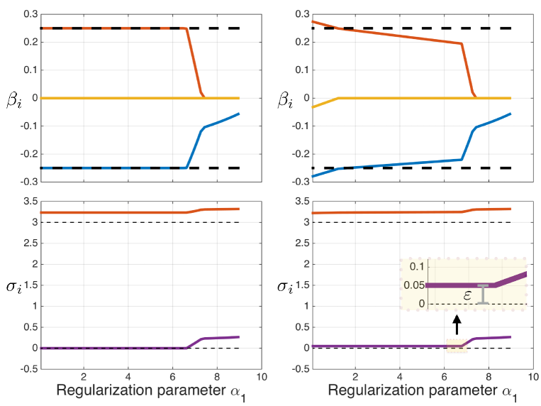
Figure 2: Generalized heteroscedastic lasso solutions for $b$ (top panel) and $s$ (bottom panel) across the $\alpha_{1}$-path. The left panels show the results of fully non-smooth perspective M-estimation. The right panels show the results for a smoothed version with $\sigma_{i}\in\left[\varepsilon,{+\infty}\right[$ for $\varepsilon=0.05$. The dashed lines mark the ground truth entries of $\overline{b}$ and $\overline{s}$.

5.1 Numerical illustrations on low-dimensional data

Our algorithmic approach to perspective M-estimation can effortlessly handle non-smooth data fitting terms. To illustrate this property, we consider a partially noiseless data formation model in low dimensions. We instantiate the data model (1.1) as follows. We consider the design matrix $X\in\mathbb{R}^{n\times p}$ with $p=3$ and sample size $n=18$. Entries in the design matrix and the noise vector $e\in\mathbb{R}^{n}$ are sampled from a standard normal distribution $\mathcal{N}(0,1)$. The matrix $C\in\mathbb{R}^{n\times n}$ is a diagonal matrix with $N=2$ groups. We set $\overline{s}=[\overline{\sigma}_{1},\overline{\sigma}_{2}]^{\top}=[3,0]^{\top}$. The $i$th diagonal entry of $C$ is set to $\overline{\sigma}_{1}$ for $i\in\{1,\ldots,8\}$ and to $\overline{\sigma}_{2}$ for $i\in\{10,\ldots,18\}$, resulting in noise-free observations for the second group. The mean shift (or outlier) vector is $\overline{o}=[0,\ldots,0]^{\top}$. The regression vector is $\overline{b}=[0.25,-0.25,0]^{\top}$. The goal is to estimate the regression vector $\overline{b}\in\mathbb{R}^{3}$ as well as the concomitant (or scale) vector $\overline{s}=[\overline{\sigma}_{1},\overline{\sigma}_{2}]^{\top}$. We consider the generalized heteroscedastic lasso of Example 3.10 with $N=2$ and $q=2$. To demonstrate the advantage of our non-smooth approach in this partially noiseless setting, we consider two variations of the model, the standard non-smooth case and a smoothed version with $D=\left[\varepsilon,{+\infty}\right[^{2}$ for $\varepsilon=0.05$. The convergence accuracy for the algorithm is set to $\epsilon=10^{-8}$. Figure 2 shows the estimates $b=[\beta_{1},\beta_{2},\beta_{3}]^{\top}$ and $s=[\sigma_{1},\sigma_{2}]^{\top}$ across the regularization path, where $\alpha_{1}\in\{0.089,\ldots,8.95\}$, with $200$ values equally spaced on a log-linear grid for both settings. The results indicate that only the heteroscedastic lasso in the non-smooth setting can recover the ground truth regression vector $\overline{b}$ (top left panel) and $\overline{\sigma}_{2}=0$ (bottom left panel). In both settings the estimate $\sigma_{1}$ is slightly overestimated (due to the finite sample size). The “smoothed” version of the heteroscedastic lasso cannot achieve exact recovery of $\overline{b}$ across the regularization path (top right panel).

5.2 Numerical illustrations for correlated designs and outliers

To illustrate the efficacy of the different M-estimators we instantiate the full data formation model (1.1) as follows. We consider the design matrix $X\in\mathbb{R}^{n\times p}$ with $p=64$ and sample size $n=75$ where each row $X_{i}$ is sampled from a correlated normal distribution $\mathcal{N}(0,\Sigma)$ with off-diagonal entries $0.3$ and diagonal entries $1$. The entries of $e\in\mathbb{R}^{n}$ are realizations of i.i.d. zero mean normal variables $\mathcal{N}(0,1)$. The matrix $C\in\mathbb{R}^{n\times n}$ is a diagonal matrix with three groups. We set $\overline{s}=[\overline{\sigma}_{1},\overline{\sigma}_{2},\overline{\sigma}_{3}]^{\top}=[5,0.5,0.05]^{\top}$. The $i$th diagonal element of $C$ is set to $\overline{\sigma}_{1}$ for $i\in\{1,\ldots,25\}$, to $\overline{\sigma}_{2}$ for $i\in\{26,\ldots,50\}$, and to $\overline{\sigma}_{3}$ for $i\in\{51,\ldots,75\}$. The mean shift vector $o\in\mathbb{R}^{n}$ contains $\lceil 0.1n\rceil=8$ non-zero entries, sampled from $\mathcal{N}(0,5)$. The entries of the regression vector $\overline{b}\in\mathbb{R}^{p}$ are set to $\overline{\beta}_{i}=-1$ for $i\in\{1,3,5\}$ and $\overline{\beta}_{i}=1$ for $i\in\{2,4,6\}$.

The presence of outliers, correlation in the design, and heteroscedasticity provides a considerable challenge for regression estimation and support recovery with standard models such as the lasso. We consider instances of the perspective M-estimation model of increasing complexity that can cope with various aspects of the data formation model. Specifically, we use the models outlined in Examples 3.10 and 3.11 (with $\alpha_{2}=0$) in homoscedastic and heteroscedastic mode. For all models, we compute the minimally achievable mean absolute error (MAE) $\|Xb-X\overline{b}\|_{1}/n$ across the $\alpha_{1}$-regularization path, where $\alpha_{1}\in\{0.254,\ldots,25.42\}$, with $50$ values equally spaced on a log-linear grid. The convergence criterion is $\epsilon=5\cdot 10^{-4}$.

Homoscedastic models. We first consider homoscedastic instances of Examples 3.10 and 3.11, in which we jointly estimate a regression vector and a single concomitant parameter in the data fitting part. We consider the generalized scaled lasso of Example 3.10 and the generalized Huber of Example 3.11 with exponents $q\in\{3/2,2\}$. Figure 3 presents the estimation results of $b$ over the relevant $\alpha_{1}$-path.

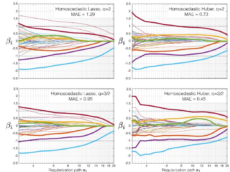
Figure 3: Generalized homoscedastic lasso and Huber solutions for $b$ when $q=2$ (top panel) and $q=3/2$ (bottom panel) across the relevant $\alpha_{1}$-path. The minimally achievable mean absolute error (MAE) is shown for all models. The six highlighted $\beta_{i}$ trajectories mark the true non-zeros entries of $\overline{b}$. The dashed black lines show the values of the true $\overline{b}$ entries.

Heteroscedastic models. We consider the same model instances as previously described but in the heteroscedastic setting. We jointly estimate regression vectors and concomitant scale parameters for each of the three groups. Figure 4 presents the results for heteroscedastic lasso and Huber estimations of $b$ across the relevant $\alpha_{1}$-path. The convergence criterion is $\epsilon=10^{-4}$.

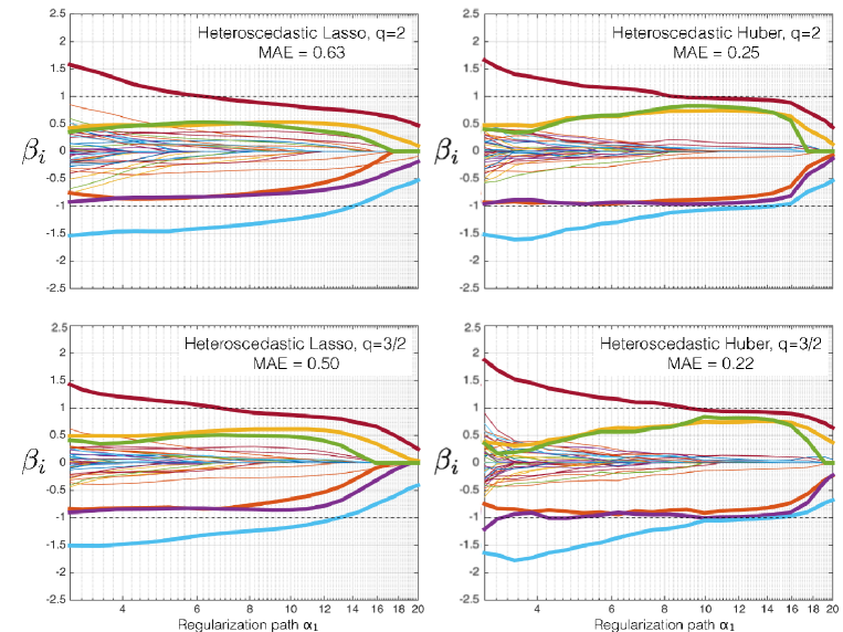
Figure 4: Generalized heteroscedastic lasso and Huber solutions for $\overline{b}$ when $q=2$ (top panel) and $q=3/2$ (bottom panel) across the relevant $\alpha_{1}$-path. The minimally achievable mean absolute error (MAE) is shown for all models. The six highlighted $\beta_{i}$ trajectories mark the true non-zeros entries of $\overline{b}$. The dashed black lines show the values of the true $\overline{b}$ entries.

The numerical experiments indicate that only heteroscedastic M-estimators are able to produce convincing $b$ estimates (as captured by lower MAE). The heteroscedastic Huber model with $q=3/2$ (see Figure 3 lower right panel) achieves the best performance in terms of MAE among all tested models.

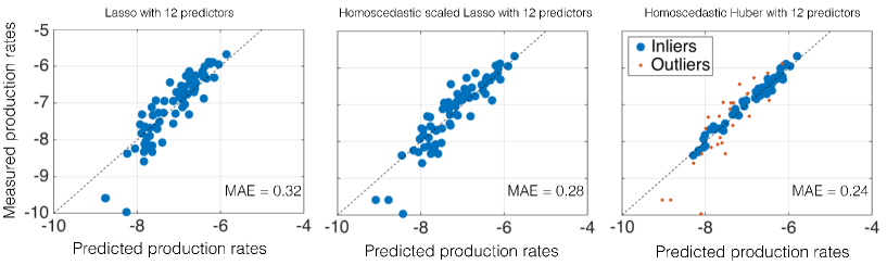
Figure 5: Standard lasso, homoscedastic lasso, and homoscedastic Huber log-production rate predictions with identical model complexity (every vector $b$ comprises twelve non-zero components) and associated MAE (computed across all samples). The Huber M-estimator identifies 26 outliers (marked in red).

5.3 Robust regression for gene expression data

We consider a high-dimensional linear regression problem from genomics [7]. The design matrix $X$ consists of $p=4088$ highly correlated gene expression profiles for $n=71$ different strains of Bacillus subtilis (B. subtilis). The response $y\in\mathbb{R}^{71}$ comprises standardized riboflavin (Vitamin B) log-production rates for each strain. The statistical task is to identify a small set of genes that is highly predictive of the riboflavin production rate. No grouping of the different strain measurements is available. We thus consider the homoscedastic models from Example 3.6 with $\alpha_{2}=0$ and Example 3.11 with $\alpha_{2}=0$. We optimize the corresponding perspective M-estimation models over the $\alpha_{1}$-path where $\alpha_{1}=[0.623,\ldots,6.23]$ with 20 values equally spaced on a log-linear grid. We compare the resulting models with the standard lasso in terms of in-sample prediction performance. Figure 5 summarizes the results for the in-sample prediction of the three different models with identical model complexity (twelve non-zero entries in $\overline{b}$). To assess model quality, we compute the minimally achievable mean absolute error (MAE) $\|Xb-y\|_{1}/n$ for these three models. The Huber model achieves significantly improved MAE (0.24) compared to lasso (0.32). The Huber models also identifies 26 non-zero components in the outlier vector $o$ (shown in red in the rightmost panel of Figure 5).

References

• [1]
• [2] A. Antoniadis, Wavelet methods in statistics: Some recent developments and their applications, Stat. Surv., vol. 1, pp. 16–55, 2007.
• [3] A. Antoniadis, Comments on: $\ell_{1}$-penalization for mixture regression models, TEST, vol. 19, pp. 257–258, 2010.
• [4] F. Bach, R. Jenatton, J. Mairal, and G. Obozinski, Optimization with sparsity-inducing penalties, Found. Trends Mach. Learn., vol. 4, pp. 1–106, 2011.
• [5] H. H. Bauschke and P. L. Combettes, Convex Analysis and Monotone Operator Theory in Hilbert Spaces, 2nd ed. Springer, New York, 2017.
• [6] L. M. Briceño-Arias and P. L. Combettes, A monotone+skew splitting model for composite monotone inclusions in duality, SIAM J. Optim., vol. 21, pp. 1230–1250, 2011.
• [7] P. Bühlmann, M. Kalisch, and L. Meier, High-dimensional statistics with a view toward applications in biology, Ann. Rev. Stat. Appl., vol. 1, pp. 255–278, 2014.
• [8] C. Chaux, P. L. Combettes, J.-C. Pesquet, and V. Wajs, A variational formulation for frame-based inverse problems, Inverse Problems, vol. 23, pp. 1495–1518, 2007.
• [9] P. L. Combettes, Perspective functions: Properties, constructions, and examples, Set-Valued Var. Anal., vol. 26, pp. 247–264, 2018.
• [10] P. L. Combettes and J. Eckstein, Asynchronous block-iterative primal-dual decomposition methods for monotone inclusions, Math. Programming, vol. 168, pp. 645–672, 2018.
• [11] P. L. Combettes and C. L. Müller, Perspective functions: Proximal calculus and applications in high-dimensional statistics, J. Math. Anal. Appl., vol. 457, pp. 1283–1306, 2018.
• [12] P. L. Combettes and J.-C. Pesquet, Proximal thresholding algorithm for minimization over orthonormal bases, SIAM J. Optim., vol. 18, pp. 1351–1376, 2007.
• [13] P. L. Combettes and J.-C. Pesquet, Stochastic quasi-Fejér block-coordinate fixed point iterations with random sweeping, SIAM J. Optim., vol. 25, pp. 1221–1248, 2015.
• [14] P. L. Combettes and V. R. Wajs, Signal recovery by proximal forward-backward splitting, Multiscale Model. Simul., vol. 4, pp. 1168–1200, 2005.
• [15] Z. J. Daye, J. Chen, and H. Li, High-dimensional heteroscedastic regression with an application to eQTL data analysis, Biometrics, vol. 68, pp. 316–326, 2012.
• [16] J. Eckstein and D. P. Bertsekas, On the Douglas-Rachford splitting method and the proximal point algorithm for maximal monotone operators, Math. Programming, vol. 55, pp. 293–318, 1992.
• [17] I. E. Frank and J. H. Friedman, A statistical view of some chemometrics regression tools, Technometrics, vol. 35, pp. 109–135, 1993.
• [18] M. Hannay and P.-Y. Deléamont, Error bounds for the convex loss Lasso in linear models, Electron. J. Stat., vol. 11, pp. 2832–2875, 2017.
• [19] M. Hebiri and S. van de Geer, The Smooth-Lasso and other $\ell_{1}+\ell_{2}$-penalized methods, Electron. J. Stat., vol. 5, pp. 1184–1226, 2011.
• [20] A. E. Hoerl, Application of ridge analysis to regression problems, Chem. Eng. Progress, vol. 58, pp. 54–59, 1962.
• [21] P. J. Huber, Robust estimation of a location parameter, Ann. Stat., vol. 35, pp. 73–101, 1964.
• [22] P. J. Huber, Robust Statistics, 1st ed. Wiley, New York, 1981.
• [23] S. Lambert-Lacroix and L. Zwald, Robust regression through the Huber’s criterion and adaptive lasso penalty, Electron. J. Stat., vol. 5, pp. 1015–1053, 2011.
• [24] S. Lambert-Lacroix and L. Zwald, The adaptive BerHu penalty in robust regression, J. Nonparametr. Stat., vol. 28, pp. 487–514, 2016.
• [25] P.-L. Lions and B. Mercier, Splitting algorithms for the sum of two nonlinear operators, SIAM J. Numer. Anal., vol. 16, pp. 964–979, 1979.
• [26] A. M. McDonald, M. Pontil, and D. Stamos, New perspectives on $k$-support and cluster norms, J. Machine Learn. Res., vol. 17, pp. 1–38, 2016.
• [27] C. A. Micchelli, J. M. Morales, and M. Pontil, Regularizers for structured sparsity, Adv. Comput. Math., vol. 38, pp. 455–489, 2013.
• [28] J. J. Moreau, Fonctions convexes duales et points proximaux dans un espace hilbertien, C. R. Acad. Sci. Paris Sér. A Math., vol. 255, pp. 2897–2899, 1962.
• [29] E. Ndiaye, O. Fercoq, A. Gramfort, V. Leclère, and J. Salmon, Efficient smoothed concomitant lasso estimation for high dimensional regression, J. Phys. Conf. Series, vol. 904, art. 012006, 2017.
• [30] A. B. Owen, A robust hybrid of lasso and ridge regression, Contemp. Math., vol. 443, pp. 59–71, 2007.
• [31] E. Raninen and E. Ollila, Scaled and square-root elastic net, Proc. IEEE Intl. Conf. Acoust. Speech Signal Process., pp. 4336–4340, 2017.
• [32] R. T. Rockafellar, Convex Analysis. Princeton University Press, Princeton, NJ, 1970.
• [33] B. Schölkopf, A. J. Smola, R. C. Williamson, and P. L. Bartlett, New support vector algorithms, Neural Computation, vol. 12, pp. 1207–1245, 2000.
• [34] Y. She and A. B. Owen, Outlier detection using nonconvex penalized regression, J. Amer. Statist. Assoc., vol. 106, pp. 626–639, 2011.
• [35] N. Städler, P. Bühlmann, and S. van de Geer, $\ell_{1}$-penalization for mixture regression models, TEST, vol. 19, pp. 209–256. 2010.
• [36] T. Sun and C. Zhang, Scaled sparse linear regression, Biometrika, vol. 99, pp. 879–898, 2012.
• [37] R. Tibshirani, Regression shrinkage and selection via the lasso, J. Roy. Stat. Soc., vol. B58, pp. 267–288, 1996.
• [38] R. J. Tibshirani, Adaptive piecewise polynomial estimation via trend filtering, Ann. Stat., vol. 42, pp. 285–323, 2014.
• [39] R. Tibshirani, M. Saunders, S. Rosset, J. Zhu, and K. Knight, Sparsity and smoothness via the fused lasso, J. Roy. Stat. Soc., vol. B67, pp. 91–108, 2005.
• [40] J. Xu and Z. Ying, Simultaneous estimation and variable selection in median regression using Lasso-type penalty, Ann. Inst. Stat. Math., vol. 62, pp. 487–514, 2010.
• [41] G. Yu and J. Bien, Estimating the error variance in a high-dimensional linear model, 2018.
https://arxiv.org/abs/1712.02412.
• [42] C. Yu and W. Yao, Robust linear regression: A review and comparison, Comm. Statist. Simulation Comput., vol. 46, pp. 6261–6282, 2017.
• [43] Z. Zou and T. Hastie, Regularization and variable selection via the elastic net, J. Royal Stat. Soc., vol. B67, pp. 301–320, 2005.