Transport coefficients of leptons in superconducting neutron star cores

Abstract

I consider the thermal conductivity and shear viscosity of leptons (electrons and muons) in the nucleon neutron star cores where protons are in the superconducting state. I restrict the consideration to the case of not too high temperatures $T\lesssim 0.35T_{\mathrm{c}p}$, where $T_{\mathrm{c}p}$ is the critical temperature of the proton pairing. In this case, lepton collisions with protons can be neglected. Charged lepton collision frequencies are mainly determined by the transverse plasmon exchange and are mediated by the character of the transverse plasma screening. In our previous works [Shternin & Yakovlev, Phys. Rev. D 75 103004 (2007); 78 063006 (2008)] the superconducting proton contribution to the transverse screening was considered in the Pippard limit $\Delta\ll\hbar qv_{\mathrm{F}p}$, where $\Delta$ is the proton pairing gap, $v_{\mathrm{F}p}$ is the proton Fermi velocity, and $\hbar q$ is the typical transferred momentum in collisions. However, for large critical temperatures (large $\Delta$) and relatively small densities (small $q$) the Pippard limit may become invalid. In the present study I show that this is indeed the case and that the older calculations severely underestimated the screening in a certain range of the parameters appropriate to the neutron star cores. As a consequence, the kinetic coefficients at $T\ll T_{\mathrm{c}p}$ are found to be smaller than in previous calculations.

I Introduction

Neutron stars (NSs) are the most compact stars known in the Universe comprising about 1.5 solar masses in a $\sim 12$ km radius sphere. In their interiors, NSs contain superdense matter of largely unknown composition Haensel et al. (2007). Their astrophysical manifestations are numerous, delivering signals in all bands of the electromagnetic spectra Kaspi (2010). Moreover, gravitational waves from a binary NS merger were detected recently Abbott et al. (2017). Understanding NSs requires modelling of various processes in their interiors. Important ingredients for this modelling are the transport coefficients of the superdense matter Schmitt and Shternin (2017); Potekhin et al. (2015).

In the present paper I discuss the thermal conductivity $\kappa$ and shear viscosity $\eta$ in NS cores of the simplest composition containing mainly neutrons (n) with admixture of protons (p), electrons (e), and muons ($\mu$). Electrons and muons form relativistic degenerate almost ideal Fermi gases, while baryons (neutrons and protons) form non-ideal strongly-interacting Fermi liquid Haensel et al. (2007). Transport coefficients are governed by the particle collisions. Leptons collide with themselves and with charged protons due to electromagnetic interaction, while collisions between baryons are mediated mainly by the strong interaction. To a good approximation, it is possible to consider lepton and baryon subsystems separately Flowers and Itoh (1979). For instance for the thermal conductivity one writes $\kappa=\kappa_{e\mu}+\kappa_{np}$. In this case, when the lepton part, $\kappa_{e\mu}$ (or $\eta_{e\mu}$), is calculated, protons (or other charged baryons if present) are treated as passive scatterers.

Currently adopted calculations of the lepton contribution to transport coefficients of non-superfluid NS core matter were performed in Refs. Shternin and Yakovlev (2007, 2008); Shternin (2008) with a proper account for the screening of electromagnetic interaction following original ideas of Heiselberg et al. (1992) and Heiselberg and Pethick (1993). Calculations of the nucleon part, $\kappa_{np}$ and $\eta_{np}$, are more uncertain since one needs to rely on a certain many-body theory of nuclear matter. Transport coefficients in the nucleon sector are studied, for instance, in Refs. Shternin et al. (2013); Kolomeitsev and Voskresensky (2015); Benhar and Valli (2007); Zhang et al. (2010) and more complete list of references can be found in the recent review Schmitt and Shternin (2017).

Nuclear matter in NS cores can be in the superfluid (paired) state due to an attractive component of the nuclear interaction Lombardo and Schulze (2001); Page et al. (2014); Haskell and Sedrakian (2017); Sedrakian and Clark (2018). Critical temperatures of the proton paring $T_{\mathrm{c}p}(n_{B})$ and neutron pairing $T_{\mathrm{c}n}(n_{B})$ depend on the baryon number density $n_{B}$. Neutrons are believed to be paired in the singlet ¹S₀ state at low densities (low Fermi momenta). In most models this type of the neutron pairing realizes in the NS inner crust, where the gas of free unbound neutrons coexists with the Coulomb lattice of ions and the degenerate electron gas. The singlet neutron pairing ceases in the core, where the ¹S₀ channel of the nuclear interaction becomes repulsive. Instead, the neutron-neutron interaction becomes attractive in the triplet ³P₂ channel leading to the anisotropic paired state in the NS core. Proton number density is $\sim 10$ times smaller than the neutron one, therefore protons in the outer core are thought to be paired in the ¹S₀ channel. In the inner core, where the proton number density increases, the ${}^{1}S_{0}$ proton pairing is thought to disappear. Calculations of critical temperature profiles for triplet neutron and singlet proton pairings in the NS core are very model-dependent Lombardo and Schulze (2001); Page et al. (2014); Gezerlis et al. (2014). Generally, the profiles $T_{\mathrm{c}p}(n_{B})$ and $T_{\mathrm{c}n}(n_{B})$ are bell-like, reaching maximum at some density within the core. The maximal critical temperature for protons is thought to be in the range $10^{9}-10^{10}$ K, while for triplet neutron superfluidity the corresponding values are found to be generally smaller, in the range of $10^{8}-5\times 10^{9}$ K. For typical temperatures in the interiors of not too young NSs, $T\sim 10^{8}$ K Yakovlev and Pethick (2004), protons in a large part of the core are expected to be in the paired and hence superconducting state.

Neutron superfluidity does not produce immediate effect on the lepton contribution to the transport coefficients. In contrast, the superfluidity of protons affects $\kappa_{e\mu}$ and $\eta_{e\mu}$ in two aspects. The first one is the damping of the lepton-proton collisions due to the reduction of the number of the proton excitations. The lepton-proton scattering is damped roughly by the exponential factor $\mathrm{exp}(-\Delta/T)$, where $\Delta$ is the gap in the proton energy spectrum. The second effect comes from the modification of the screening of the electromagnetic interactions which affects collisions between all charged particles including unpaired ones (leptons in the present case). Both these effects were investigated in Refs. Shternin and Yakovlev (2007, 2008). In these papers, the proton contribution to screening was taken in the so-called Pippard limit, $qv_{\mathrm{F}p}\gg\Delta$, where $v_{\mathrm{F}p}$ is the proton Fermi velocity and $q$ is the momentum transfer in collisions, both of which increase with density. In the present paper I show that this limit is inapplicable for the wide range of conditions relevant for NS cores, i.e. for not too high densities (small $qv_{\mathrm{F}p}$) or for relatively high gap values (high $T_{\mathrm{c}p}$). The opposite, London limit, $\Delta\gg qv_{\mathrm{F}p}$ can be equally relevant for lepton scattering, and the transition between two limiting cases occurs roughly at the transition between the superconductors of the first and second kind.

The paper is organized as follows. In Sec. II the general formalism needed to calculate transport coefficients of npe$\mu$ matter of NS cores is briefly outlined and the results of Refs. Shternin and Yakovlev (2007, 2008) for a normal (non-superfluid) case are reviewed. In Sec. III.1 the plasma screening properties in presence of the proton pairing are discussed and in Sec. III.2–III.4 transport coefficients in this case are calculated. The results are summarized and discussed in Sec. IV. I conclude in Sec. V.

The consideration in this study is limited to small temperatures, $T\lesssim 0.35T_{\mathrm{c}p}$ and the effects of magnetic fields are not included.

II General expressions

Transport coefficients in NS cores can be calculated in the framework of the transport theory of Fermi liquids Baym and Pethick (1991) adapted for multicomponent systems Flowers and Itoh (1979); Anderson et al. (1987); Schmitt and Shternin (2017). Below I closely follow Refs. Shternin and Yakovlev (2007, 2008) and omit the details.

Thermal conductivity $\kappa_{c}$ and shear viscosity $\eta_{c}$ of particle species $c$ can be conveniently written as

$$\kappa_{c}=\frac{\pi^{2}Tn_{c}}{3m^{*}_{c}}\tau^{\kappa}_{c},\quad\eta_{c}=\frac{p_{{\rm F}c}^{2}n_{c}}{5m^{*}_{c}}\tau^{\eta}_{c},$$ (1)

where $n_{c}$ is the number density of the corresponding species, $p_{\mathrm{F}c}$ is their Fermi momentum, and $m_{c}^{*}$ is their effective mass on the Fermi surface. The quantities $\tau^{\kappa,\eta}_{c}$ are effective relaxation times which are generally not the same for different transport problems (thermal conductivity and shear viscosity in present case, as indicated by the corresponding superscripts here and in the rest of the paper) and need to be determined from the transport theory.

The effective relaxation times $\tau^{\kappa,\eta}_{c}$ are found from the solution of a system of coupled transport equations. However, for strongly degenerate matter in NS cores it is enough to rely on the simplest variational solution of this system Shternin and Yakovlev (2007, 2008); Schmitt and Shternin (2017) (see, however, Sec. III.4). Then the problem of finding effective relaxation times reduces to a system of algebraic equation

$$1=\sum_{i}\left(\nu_{ci}\tau_{c}+\nu_{ci}^{\prime}\tau_{i}\right),$$ (2)

where indices $c$, $i$ number particles species and the effective collision frequencies $\nu_{ci}$ and $\nu^{\prime}_{ci}$ are related to the transport cross-sections as shown below. The correction to the variational solution for lepton transport coefficients in normal matter was found to be within 10% Shternin and Yakovlev (2007, 2008) which is unimportant for practical applications. The frequencies $\nu_{ci}$ describe relaxation due to collisions of particle species $c$ with all other particles including the passive scatterers. The primed quantities $\nu_{ci}^{\prime}$ are the mixing terms. Notice, that the summation in Eq. (2) is carried over all particle species in both terms, so that the actual collision frequency for collisions of like particles is $\nu_{cc}+\nu_{cc}^{\prime}$. These two parts are kept separated for convenience.

Collision frequencies are calculated by integrating the squared matrix element $|M_{ci}|^{2}$ of corresponding interaction over the available phasespace with certain phase factors. Consider particle collisions $c,i\to c^{\prime},i^{\prime}$. Primes here mark the particle states after the collision. Due to a strong degeneracy, the particle states before and after the collision can be placed on the respective Fermi surfaces whenever possible, hence the absolute values of input and output momenta are fixed: $p_{c}=p_{c^{\prime}}=p_{\mathrm{F}c}$ and $p_{i}=p_{i^{\prime}}=p_{\mathrm{F}i}$. Owing to the momentum conservation, the relative orientation of the four participating momenta is fixed by two angular variables. In case of electromagnetic collisions, the convenient pair of variables is the absolute value of the transferred momentum $q$, where $\mathbf{q}=\mathbf{p}_{c^{\prime}}-\mathbf{p}_{c}$, and the angle $\phi$ between the vectors $\mathbf{p}_{c}+\mathbf{p}_{c^{\prime}}$ and $\mathbf{p}_{i}+\mathbf{p}_{i^{\prime}}$. Notice, that these two vectors are transverse to $\mathbf{q}$. It is instructive to introduce the spin-averaged squared matrix element ${\cal Q}_{ci}(\omega,q,\phi)=(1+\delta_{ci})^{-1}\sum_{\mathrm{spins}}|M_{ci}|^{2}/4$, where the factor $(1+\delta_{ci})^{-1}$ is included in order to avoid double counting of the same collisions when antisymmetrized amplitudes are used. In general, ${\cal Q}_{ci}$ depends also on the transferred energy $\omega=\epsilon_{c^{\prime}}-\epsilon_{c}$, where $\epsilon_{c}$ is the particle energy. In degenerate matter, $\omega$ is of the order of $T$ and therefore small. In the limit $\omega\ll qv_{\mathrm{F}i}$, the collision frequencies to be used in (2) are Shternin and Yakovlev (2007, 2008)

$$\nu^{\kappa}_{ci} = \frac{3T^{2}m_{c}^{*}m_{i}^{*2}}{4\pi^{4}p_{\mathrm{F}c}}$$ (3)

$$\times\left\langle\frac{\omega^{2}}{\pi^{2}T^{2}}\left(1+\left[\frac{\pi^{2}T^{2}}{3\omega^{2}}-\frac{1}{6}\right]\frac{q^{2}}{p_{\mathrm{F}c}^{2}}\right)\,{\cal Q}_{ci}\right\rangle,$$

$${\nu^{\prime}}^{\kappa}_{ci} = -\frac{3T^{2}p_{\mathrm{F}i}m_{c}^{*2}m_{i}^{*}}{4\pi^{4}p_{\mathrm{F}c}^{2}}$$

$$\times\left\langle\frac{\omega^{2}}{\pi^{2}T^{2}}\sqrt{\left(1-\frac{q^{2}}{4p_{\mathrm{F}c}^{2}}\right)\left(1-\frac{q^{2}}{4p_{\mathrm{F}i}^{2}}\right)}{\cos\phi}\,{\cal Q}_{ci}\right\rangle,$$

$$\nu^{\eta}_{ci}=\frac{3T^{2}m_{c}^{*}m_{i}^{*2}}{4\pi^{4}p_{\mathrm{F}c}}\left\langle{\frac{q^{2}}{p_{\mathrm{F}c}^{2}}}\left(1-\frac{q^{2}}{4p_{\mathrm{F}c}^{2}}\right)\,{\cal Q}_{ci}\right\rangle,$$ (5)

$${\nu^{\prime}}^{\eta}_{ci} = -\frac{3T^{2}p_{\mathrm{F}i}m_{c}^{*2}m_{i}^{*}}{4\pi^{4}p_{\mathrm{F}c}^{2}}$$

$$\times\left\langle{\frac{q^{2}}{p_{\mathrm{F}c}^{2}}}\sqrt{\left(1-\frac{q^{2}}{4p_{\mathrm{F}c}^{2}}\right)\left(1-\frac{q^{2}}{4p_{\mathrm{F}i}^{2}}\right)}{\cos\phi}\,{\cal Q}_{ci}\right\rangle,$$

where the angular brackets denote phase-space integration

$$\langle\cdot\rangle=\int\limits_{0}^{\infty}dw\,\frac{\left(w/2\right)^{2}}{\mathrm{sinh^{2}}\left(w/2\right)}\int\limits_{0}^{q_{m}}dq\int\limits_{0}^{\pi}d\phi\,\cdot\,,$$ (7)

$w=\omega/T$, and $q_{m}=\mathrm{min}(2p_{\mathrm{F}c},2p_{\mathrm{F}i})$. Dependence of ${\cal Q}_{ci}$ on $\omega$ determines the temperature behavior of collision frequencies and hence of the corresponding transport coefficients. In traditional transport theory of Fermi systems, the transition probability is assumed to be independent of $\omega$. Then each collision frequency in Eqs. (3)–(II) obeys $\nu_{ci}\propto T^{2}$ scaling which according to Eqs. (1)–(2) results in standard dependencies $\kappa\propto T^{-1}$ and $\eta\propto T^{-2}$. These relations hold, for instance, for the transport coefficients in the nucleon sector, e.g. Schmitt and Shternin (2017).

Consider leptonic (electrons and muons) subsystem. Leptons collide with all charged particles due to electromagnetic interaction. The matrix element of this interaction can be written as a sum of the longitudinal and transverse parts

$$M_{ci}=4\pi\alpha_{f}\left(\frac{J^{(0)}_{c}J^{(0)}_{i}}{q^{2}+\Pi_{l}(\omega,q)}-\frac{\mathbf{J}_{c,t}\cdot\mathbf{J}_{i,t}}{q^{2}-\omega^{2}+\Pi_{t}(\omega,q)}\right)\,,$$ (8)

where $\alpha_{f}\approx 1/137$ is the fine structure constant, $J^{(0)}_{c}$ and $\mathbf{J}_{c,t}$ are time-like and transverse (with respect to $\mathbf{q}$) space-like components of the transition current, respectively, and $\Pi_{l}$ and $\Pi_{t}$ are the longitudinal and transverse polarization functions, respectively.

The transition four-current in Eq. (8) is $J^{\lambda}_{c}=Z_{c}\bar{u}(\mathbf{p}_{c^{\prime}})\gamma^{\lambda}u(\mathbf{p}_{c})/(2\sqrt{\epsilon_{c}\epsilon_{c^{\prime}}})$, where $Z_{c}$ is the charge number of the particle species $c$, $\gamma^{\lambda}$ is a Dirac matrix, and $u(\mathbf{p}_{c})$ is the Dirac spinor. Performing spin summations (in the limit $\omega\ll qv_{\mathrm{F}i}$), one obtains Shternin and Yakovlev (2007, 2008); Alford et al. (2014)

$${\cal Q}_{ci}=16\pi^{2}\alpha_{f}^{2}Z_{c}^{2}Z_{i}^{2}\left(\frac{L_{l}}{\left|q^{2}+\Pi_{l}(\omega,q)\right|^{2}}-2\mathrm{Re}\frac{v_{\mathrm{F}c}v_{\mathrm{F}i}L_{tl}}{(q^{2}+\Pi_{l}(\omega,q))(q^{2}+\Pi_{t}(\omega,q))^{*}}+\frac{v_{\mathrm{F}c}^{2}v_{\mathrm{F}i}^{2}L_{t}}{\left|q^{2}+\Pi_{t}(\omega,q)\right|^{2}}\right),$$ (9)

where the numerators are

$$L_{l} = \left(1-\frac{q^{2}}{4m_{c}^{*2}}\right)\left(1-\frac{q^{2}}{4m_{i}^{*2}}\right),$$ (10)

$$L_{tl} = \sqrt{\left(1-\frac{q^{2}}{4p_{\mathrm{F}c}^{2}}\right)\left(1-\frac{q^{2}}{4p_{\mathrm{F}i}^{2}}\right)}{\cos\phi},$$ (11)

$$L_{t} = \left(1-\frac{q^{2}}{4p_{\mathrm{F}c}^{2}}\right)\left(1-\frac{q^{2}}{4p_{\mathrm{F}i}^{2}}\right){\cos^{2}\phi}$$ (12)

$$+\frac{q^{2}}{4p_{\mathrm{F}c}^{2}}+\frac{q^{2}}{4p_{\mathrm{F}i}^{2}}.$$

In case of identical particles, ${\cal Q}_{cc}$ also contains an exchange contribution from the interference between two scattering channels with the final states interchanged. However, for the electromagnetic collisions, small momentum transfer $q\ll p_{\mathrm{F}c}$ dominates the scattering, interference corrections are of the next order in $q$ and are found to be negligible Shternin and Yakovlev (2007, 2008).

As follows from Eq. (9), ${\cal Q}_{ci}$ has contributions from longitudinal, transverse, and mixed parts of electromagnetic interaction. Moreover, due to a specific $\cos\phi$ dependence in Eqs. (3)–(II) and (10)–(11), the mixed term does not contribute to ‘direct’ collision frequencies (3) and (5), so one can write $\nu_{ci}=\nu_{ci}^{l}+\nu_{ci}^{t}$. In contrast, only the mixed term contributes to the primed collision frequencies, $\nu_{ci}^{\prime}=\nu_{ci}^{tl}$ Shternin and Yakovlev (2007, 2008). In the non-relativistic limit $v_{\mathrm{F}c/i}\ll 1$ and the transverse part of the interaction is unimportant. However, it turns out that for relativistic particles this part gives the dominant contribution because of the weaker screening. The leading $q^{-4}$ dependence of ${\cal Q}_{ci}$ is regularized at small $q$ by the polarization functions $\Pi_{l}$ and $\Pi_{t}$ which play the central role in determining the collision frequencies. Characters of the longitudinal and transverse screening are very different. It is enough to consider screening in the limits of small $q\ll p_{\mathrm{F}i}$ and $\omega\ll\mu_{i}$, where $\mu_{i}$ is the chemical potential of the i species, and also in the static limit $\omega\ll qv_{\mathrm{F}i}$. Then the longitudinal part of the interaction is screened on a static Thomas-Fermi scale

$$\Pi_{l}(\omega,q)=q_{\mathrm{TF}}^{2}\equiv\frac{4\alpha_{f}}{\pi}\sum_{i}Z_{i}^{2}m_{i}^{*}p_{\mathrm{F}i},$$ (13)

where $q_{\mathrm{TF}}$ is the Thomas-Fermi screening momentum. In contrast, the transverse screening is dynamical

$$\Pi_{t}(\omega,q)=i\;\frac{\pi}{4}\frac{\omega}{q}q_{t}^{2}\equiv i\;\frac{\omega}{q}\alpha_{f}\sum_{i}Z_{i}^{2}p^{2}_{\mathrm{F}i},$$ (14)

where $q_{t}$ is a characteristic transverse momentum. Therefore the screening scale of the transverse part of the interaction is $\sim(\omega q_{t}^{2})^{1/3}\ll q_{\mathrm{TF}}$ [examine the denominator in the third term in Eq. (9)]. This leads to dominant contribution of the transverse interaction to the collision frequencies, $\nu_{ci}^{t}\gg\nu_{ci}^{l},\,\nu_{ci}^{tl}$. As a consequence, the system (2) decouples, and in the leading order $\tau_{c}=\left(\sum_{i}\nu_{ci}^{t}\right)^{-1}$. Retaining only the transverse contribution and the leading order in $q$ in Eqs. (3)–(II), one gets the following expressions for the lepton thermal conductivity and shear viscosity in normal matter Shternin and Yakovlev (2007, 2008); Schmitt and Shternin (2017)

$$\kappa_{e\mu} = \frac{\pi^{2}}{54\zeta(3)}\frac{p_{\mathrm{F}e}^{2}+p_{\rm F\mu}^{2}}{\alpha_{f}},$$ (15)

$$\eta_{e\mu} = \frac{1.1}{\alpha_{f}}\frac{n_{e}^{2}+n_{\mu}^{2}}{q_{t}^{1/3}}{T^{-5/3}},$$ (16)

where $\zeta(3)$ is the Riemann zeta-function. Notice the unusual temperature behavior of $\kappa_{e\mu}$ and $\eta_{e\mu}$ in comparison to the standard Fermi-liquid results. This is a consequence of the dynamical character of the transverse screening. The different powers of $T$ in Eqs. (15) and (16) are traced back to the different leading orders in $q$ for the thermal conductivity ($q^{0}$) and shear viscosity ($q^{2}$) problems in Eqs. (3)–(II). Expression (15) is a good approximation to the exact result, which includes all contributions to collision frequencies. For the shear viscosity, the dominance of the transverse part of interaction is not so strong, and Eq. (16) can actually result in a strong overestimation of the shear viscosity coefficient Shternin and Yakovlev (2008); Kolomeitsev and Voskresensky (2015). In this case all terms need to be retained.

III Lepton transport coefficients in superconducting NS cores

Shternin and Yakovlev (2007, 2008) also calculated $\kappa_{e\mu}$ and $\eta_{e\mu}$ in the case when the protons are in the paired state. They noticed that the proton pairing changes the character of transverse plasma screening from the dynamical to the static one restoring the Fermi-liquid behavior of transport coefficients. Below I show that this qualitative result is correct, but the treatment of screening in Refs. Shternin and Yakovlev (2007, 2008) was incomplete. For simplicity, I restrict myself to the case of well-developed superconductivity $T\lesssim 0.2\Delta$. For ${}^{1}S_{0}$ pairing, dependence of the superfluid gap on temperature can be approximated as Levenfish and Yakovlev (1994)

$$\frac{\Delta}{T}=\sqrt{1-t}\left(1.456-\frac{0.157}{\sqrt{t}}+\frac{1.764}{t}\right),$$ (17)

where $t=T/T_{\mathrm{c}p}$. Thus the condition $T\lesssim 0.2\Delta$ translates to $T/T_{\mathrm{c}p}\lesssim 0.35$. In this case, first of all, lepton-proton collisions can be neglected, and, second, the zero-temperature limit for the proton polarization function can be used. Provided high expected values of $T_{\mathrm{c}p}$, this limit is comfortably satisfied at $T\lesssim 10^{8}$ K.

III.1 Plasma screening in presence of proton pairing

Pairing of protons, which are charged particles, modifies the screening of the electromagnetic interaction. Up to the order $\Delta/\mu_{p}$, the static longitudinal screening does not change Gusakov (2010); Arseev et al. (2006) and $\Pi_{l}$ is given by Eq. (13). In contrast, the transverse screening modifies. At low $T$, the dominant contribution to screening comes from protons. In the zero-temperature limit $T\to 0$ in the Bardeen-Cooper-Schrieffer (BCS) theory the static ($\omega\to 0$) transverse polarization function can be written as Lifshitz and Pitaevskii (1980)

$$\Pi_{t}(0,q)=q_{M}^{2}J(\zeta),$$ (18)

where $\zeta=qv_{\mathrm{F}p}/\Delta=\pi q\xi$, $\xi$ is the coherence length, and $q_{M}$ is the Meissner screening momentum (Meissner mass)

$$q_{M}^{2}=\frac{4\alpha_{f}}{3\pi}p_{\mathrm{F}p}^{2}v_{\mathrm{F}p}.$$ (19)

The function $J(\zeta)$ in Eq. (18) is Lifshitz and Pitaevskii (1980)

$$J(\zeta) = \frac{3}{8}\int\limits_{-\infty}^{\infty}d\eta\int\limits_{-1}^{1}\frac{dx\,(1-x^{2})}{\sqrt{\eta^{2}+1}\left(\eta^{2}+1+(\zeta x)^{2}/4\right)}$$ (20)

$$= \frac{3}{4}\int\limits_{-1}^{1}dx\,(1-x^{2})\,\frac{2{\rm ArcSinh}(\zeta x/2)}{\zeta x\sqrt{1+(\zeta x)^{2}/4}}.$$

In principle, the integration over $x$ in the second line in Eq. (20) can be performed analytically with the result being expressed via the polylogarithmic functions.

Figure 1: Proton contribution to the zero-temperature transverse polarization function in the static limit. Polarization function is normalized to $q_{M}^{2}$. Dashed line shows the asymptote in the Pippard limit.

The function $J(\zeta)$ is plotted in Fig. 1. At small $\zeta$ (small momentum $q\ll\xi^{-1}$), which corresponds to the London limit, $J(\zeta)=1$. In this limit, the transverse screening is independent of $\Delta$ and the screening momentum is equal to $q_{M}$. The real transverse photons obey the Meissner mass $q_{M}$ in this limit. This leads to the Meissner effect in superconductors. In the opposite, Pippard limit, $\zeta\gg 1$ and $\Pi_{t}$ is inversely proportional to $\zeta$ as shown by the dashed line in Fig. 1. The asymptotic expression in the Pippard limit reads $J(\zeta)=3\pi^{2}/(4\zeta)$. In this limit, the characteristic transverse screening momentum is $q_{P}=(3\pi^{2}\Delta q_{M}^{2}/(4v_{\mathrm{F}p}))^{1/3}$. This expression resembles the screening momentum in the non-superfluid case, with $\Delta$ in place of $\omega$ and $q_{M}$ in place of $q_{t}$. In the Pippard limit, contrary to the London limit, the screening depends on $\Delta$.

In Fig. 2, the characteristic transverse screening momenta $q_{M}$ (dashed lines) and $q_{P}$ (dash-dotted lines for $T_{\mathrm{c}p}=10^{9}$ K and double-dot-dashed lines for $T_{\mathrm{c}p}=10^{10}$ K) are compared with the longitudinal screening momentum $q_{\mathrm{TF}}$ (solid lines). The momenta in the plot are normalized to $2p_{\mathrm{F}e}$, which is the maximum momentum transfer in electron-electron collisions. Thick and thin lines correspond to two widely used equations of state (EOSs) of dense nucleon matter in NS cores. Namely, by the abbreviation HHJ (thick lines) I denote the EOS constructed by Heiselberg and Hjorth-Jensen (1999) as an analytical parameterization of the variational EOS by Akmal et al. (1998). Specifically, I use the model with the parameter $\gamma=0.6$ of Ref. Heiselberg and Hjorth-Jensen (1999); this model was designated as APR I in Ref. Gusakov et al. (2005) and the NS properties with such EOS can be found there. With thin lines I show the results for one of the EOSs based on the Brussels-Skyrme nucleon interaction functionals, namely the BSk21 model Potekhin et al. (2013). Both EOSs satisfy the equilibrium conditions with respect to the weak processes. Unless otherwise indicated, the proton effec1tive mass is set to $m_{p}^{*}=0.8m_{u}$, where $m_{u}$ is the nucleon mass unit. Two EOSs are different in the particle fractions, however the results shown in Fig. 2 are qualitatively same. As in the normal matter, characteristic transverse screening momenta ($q_{M}$ or $q_{P}$) are much smaller than the longitudinal one. As a consequence, the transverse part of the interaction dominates in the presence of proton superconductivity as well.

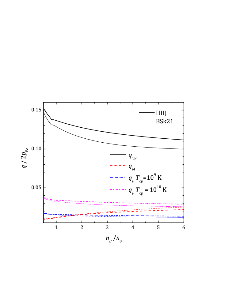
Figure 2: (Color online). Ratios of characteristic screening momenta to $2p_{\mathrm{F}e}$ versus baryon density (in units of the nuclear saturation density $n_{0}=0.16\leavevmode\nobreak\ {\rm fm}^{-3}$) for two EOSs desribed in the text. Thick lines correspond to the HHJ EOS, while thin lines show the results for the BSk21 EOS. Solid lines show the longitudinal (Thomas-Fermi) screening momentum $q_{\mathrm{TF}}$, dashed lines give the Meissner momentum $q_{M}$. Dash-dotted and double-dot-dashed lines show the characteristic screening momenta in Pippard limit for $T_{\mathrm{c}p}=10^{9}$ K and $10^{10}$ K, respectively.

In Refs. Shternin and Yakovlev (2007, 2008) it was assumed that the typical transferred momentum $q$ is not so small, so that the Pippard limit gives appropriate description of the transverse plasma screening in NS cores. In fact, which limit, London or Pippard, gives the dominant contribution depends on the value of $\zeta$ at $q=q_{M}$. This point was overlooked in Refs. Shternin and Yakovlev (2007, 2008). It is hence convenient to introduce the parameter $A\equiv\zeta(q=q_{M})=v_{\mathrm{F}p}q_{M}/\Delta$. In the BCS approximation, this parameter is related to the familiar Ginzburg-Landau coherence parameter $\varkappa$, namely $\varkappa=\lambda_{L}/\xi=\pi/A$, where $\lambda_{L}=q_{M}^{-1}$ is the London penetration depth. The value of $\varkappa$ determines the superconductivity type. The transition from type I superconductor to type II superconductor occurs at $\varkappa>1/\sqrt{2}$ as type-I Tilley and Tilley (1990); Lifshitz and Pitaevskii (1980), which corresponds to $A<\sqrt{2}\pi\approx 4.4$. The parameter $A$ can be written as

$$A=1.12\left(\frac{x_{p}}{0.1}\right)^{5/6}\left(\frac{n_{B}}{n_{0}}\right)^{5/6}\left(\frac{m^{*}_{p}}{m_{u}}\right)^{-3/2}\frac{0.5\leavevmode\nobreak\ {\rm MeV}}{\Delta},$$ (21)

where $n_{0}=0.16\leavevmode\nobreak\ {\rm fm}^{-3}$ is the nuclear saturation density. In Fig. 3, the parameter $A$ is plotted for two EOSs discussed above and for $\Delta=1$ MeV. This corresponds to $T_{\mathrm{c}p}\approx 6.5\times 10^{9}$ K [see Eq. (17) at $T=0$]. For this large $\Delta$, most of the core forms type-II superconductor Baym et al. (1969). Since $A$ is inversely proportional to $\Delta$, it is higher for lower $\Delta$ (lower $T_{\mathrm{c}p}$). For the NS core conditions, $A$ can vary in the range $0.1\div 100$. Figure 1 shows that these values correspond to the intermediate region between the London and Pippard limits, thus one can expect that neither of these limits is strictly applicable in NS cores, and the general form of $\Pi_{t}$ should be used for calculating the transport coefficients. This is demonstrated in the next Section.

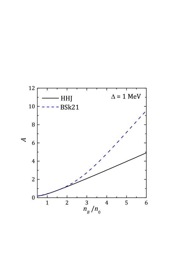
Figure 3: (Color online). The coherence scale parameter $A$ as a function of the total baryon density for two selected EOSs. Effective masses are set to $m^{*}_{p}=0.8m_{u}$ and $\Delta=1$ MeV.

III.2 Calculation of transport coefficients in the leading order

According to the discussion in Secs. II and III.1 (see also Fig. 2), the dominant contribution to the lepton collision frequencies comes from the transverse part of the electromagnetic interaction. In addition, since the screening is weak, the lowest order in $q$ in Eqs. (3)–(II), (9)–(12) gives the leading contribution to transport coefficients. In order to calculate the transverse collision frequencies $\nu_{ci}^{t}$, the integrals

$$I^{t}_{n}(A,q_{M})=\int_{0}^{q_{m}}\frac{dq\,q^{n}}{(q^{2}+q_{M}^{2}J(\zeta))^{2}}$$ (22)

are needed. The exponent $n=0$ in Eq. (22) gives the leading order contribution for the thermal conductivity problem, while for the shear viscosity the leading order is given by $n=2$ (Sec. II). Retaining only the leading contributions one gets the following results for the lepton thermal conductivity and shear viscosity

$$\kappa_{e\mu}^{t,\,\mathrm{Lead}} = \frac{5}{72\pi\alpha^{2}_{f}{T}}\left[I^{t}_{0}(A,q_{M})\right]^{-1},$$ (23)

$$\eta_{e\mu}^{t,\,\mathrm{Lead}} = \frac{3\pi}{10\alpha_{f}^{2}T^{2}}\frac{n_{e}^{2}+n_{\mu}^{2}}{p_{\mathrm{F}e}^{2}+p_{\mathrm{F}\mu}^{2}}\left[I^{t}_{2}(A,q_{M})\right]^{-1}.$$ (24)

Let us analyze an asymptotic behavior of the integrals (22). In the weak-screening limit $q_{M}\ll q_{m}$ it is enough to extend the upper integration limit to infinity. Then, the low-$A$ asymptote becomes

$$I^{t}_{n}=\frac{\pi}{4q_{M}^{3-n}},\quad A\ll 1,$$ (25)

while the high-$A$ asymptotes are

$$I^{t}_{0}=\frac{4A}{9\pi^{2}q_{M}^{3}},\quad I^{t}_{2}=\frac{4A^{1/3}}{9q_{M}}\,\frac{2^{2/3}\pi^{1/3}}{3^{5/6}},\quad A\gg 1.$$ (26)

Remarkably, the low-$A$ asymptote (25), which corresponds to the London limit, is independent of $A$ and hence of $\Delta$. This is a consequence of the independence of the Meissner momentum $q_{M}$ of the gap value. The case of large $A$, Eq. (26), corresponds to the Pippard limit that was employed in Refs. Shternin and Yakovlev (2007, 2008). In the intermediate case, the integrals $I_{0}^{t}$ and $I_{2}^{t}$ were fitted by the analytic expressions to facilitate their use in applications. These expressions are given in the Appendix. Substituting the limiting expressions (25)–(26) into Eqs. (23)–(24), one obtains the asymptotic expressions for the thermal conductivity and shear viscosity

$$\kappa_{e\mu}^{\mathrm{Lon}} = \frac{5q_{M}^{3}}{18\pi^{2}\alpha_{f}^{2}T},$$ (27)

$$\eta_{e\mu}^{\mathrm{Lon}} = \frac{6q_{M}}{5\alpha_{f}^{2}\,T^{2}}\frac{n_{e}^{2}+n_{\mu}^{2}}{p_{\mathrm{F}e}^{2}+p_{\mathrm{F}\mu}^{2}},$$ (28)

$$\kappa_{e\mu}^{\mathrm{Pip}} = \frac{5\,p_{\mathrm{F}p}^{2}}{24\alpha_{f}}\frac{\Delta}{{T}},$$ (29)

$$\eta_{e\mu}^{\mathrm{Pip}} = \frac{1.71\,p_{\mathrm{F}p}}{\alpha_{f}^{5/3}\,T^{2}}\frac{n_{e}^{2}+n_{\mu}^{2}}{p_{\mathrm{F}e}^{2}+p_{\mathrm{F}\mu}^{2}}{\left(\frac{\Delta}{p_{\mathrm{F}p}c}\right)^{1/3}},$$ (30)

where the superscripts Lon and Pip correspond to the London and Pippard approximations to $\Pi_{t}$, respectively.

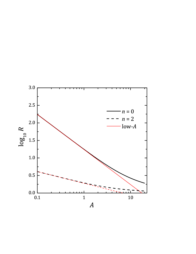
Figure 4: (Color online). The ratio $R(A)$ for $n=0$ (solid lines) and $n=2$ (dashed lines). Thin lines represent the low-$A$ approximation (25).

Comparing the expressions (25) and (26) one can roughly estimate that the crossover between the two limiting cases occurs at $A\approx 17.5$ for $n=0$ and at $A\approx 6.8$ for $n=2$. From Fig. 3, one concludes that for large $\Delta\sim 1$ MeV or for small $n_{B}$ if $\Delta$ is lower, the Pippard limit used in Refs. Shternin and Yakovlev (2007, 2008) is inapplicable. To illustrate the possible degree of inaccuracy of the older results, let us construct the ratio $R(A)$ of the leading contribution to transverse collision frequency to those calculated in the Pippard limit: $\nu_{t}^{\mathrm{Lead}}=\nu_{t}^{\mathrm{Pip}}R(A)$. This ratio is plotted as a function of $A$ in Fig. 4 for $n=0$ (thermal conductivity, solid lines) and $n=2$ (shear viscosity, dashed lines). The plot clearly shows underestimation of the collision frequencies, and, hence overestimation of the transport coefficients by the Pippard limiting values (29)–(30). For small $A$ and $n=0$ this overestimation reaches two orders of magnitude. For the shear viscosity problem ($n=2$), the overestimation is modest because of the weaker dependence of the collision frequencies on the screening momentum (Sec. II). Thin lines in Figure 4 show the same factors, where the London asymptotic expression for collision frequencies is used in place of $\nu^{t,\mathrm{Lead}}$. One concludes, that the London limit for screening is appropriate in the case of type-II superconductivity, but for large values of $A$ it becomes inapplicable. Fig. 4 shows that both asymptotic limits generally underestimate the collision frequencies and overestimate the transport coefficients. This is because of an overestimation of the screening at large $q$ by the London expression and at small $q$ by the Pippard expression, see Fig. 1.

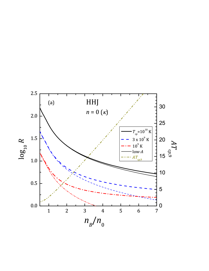
Figure 5: (Color online). The ratios $R$ for (a) thermal conductivity ($n=0$) and (b) shear viscosity ($n=2$) as function of $n_{B}$ for the HHJ equation of state and three values of $T_{\mathrm{c}p}=10^{10}$ K (solid lines), $3\times 10^{9}$ K (dashed lines), and $10^{9}$ K (dash-dotted lines). Thin lines give low-$A$ approximation, where the interaction is screened by the pure Meissner mass. Double-dot-dashed lines show with right vertical scales the combination $AT_{\mathrm{c}p,9}$ which is independent of $T_{\mathrm{c}p}$. Here $T_{\mathrm{c}p,\,9}\equiv T_{\mathrm{c}p}/(10^{9}\leavevmode\nobreak\ \mathrm{K})$.

For illustration, the same ratios $R$ are plotted in Fig. 5 now as functions of the baryon density for the HHJ EOS and three values of $T_{\mathrm{c}p}=10^{10}$ K (solid lines), $3\times 10^{9}$ K (dashed lines), and $10^{9}$ K (dash-dotted lines). Figure 5(a) shows the results appropriate for the thermal conductivity ($n=0$), while for the shear viscosity problem ($n=2$), $R$ is shown in Fig. 5(b). Like in Fig. 4, thin lines give the ratio $R$ calculated with London limiting expression. For the highest shown critical temperature, $T_{\mathrm{c}p}=10^{10}$ K, $R$ is largest and the London expression is a good approximation for $n=0$ in the whole shown range of densities and for $n_{B}\lesssim 3n_{0}$ for $n=2$. With decreasing $T_{\mathrm{c}p}$ (increasing $A$), the ratio $R$ lowers down and the applicability range of the London limiting expression shifts to lower densities. For instance, for $T_{\mathrm{c}p}=10^{9}$ K and $n=2$ the London approximation is always inaccurate, as seen from a comparison of thin and thick dash-dotted lines in Fig. 5(b).

III.3 Kinematic corrections

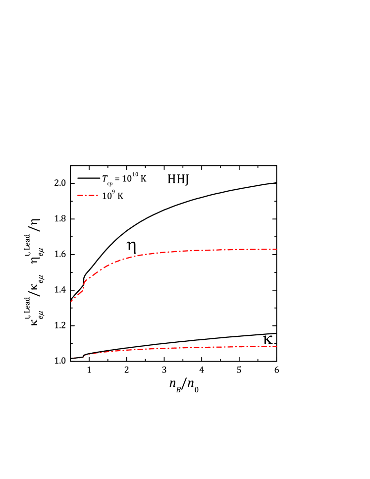
Figure 6: (Color online). Comparison of the thermal conductivity and shear viscosity in the leading approximation, Eqs. (23)–(24), to the results of complete calculations. Upper pair of curves shows the ratio $\eta^{t,\,\mathrm{Lead}}_{e\mu}/\eta_{e\mu}$, while lower pair of curves marked $\kappa$ shows $\kappa^{t,\,\mathrm{Lead}}_{e\mu}/\kappa_{e\mu}$. Results for the HHJ EOS are shown and for two values of the proton critical temperature. $T_{\mathrm{c}p}=10^{10}$ K (solid lines) and $10^{9}$ K (dashed lines). Variational solutions are employed. See text for details.

In the previous section the leading order contribution to the collision frequencies was discussed. However, as was mentioned at the end of the Sec. II, this approximation can be inaccurate, especially for the shear viscosity and in principle the full result that follows from Eqs. (2)–(II) and (9)–(12) shall be used Shternin and Yakovlev (2008); Kolomeitsev and Voskresensky (2015); Schmitt and Shternin (2017). The main corrections come from the inclusion of the longitudinal part of the interaction, and from the kinematic corrections of high-$q$ powers in Eqs. (3)–(II) and (10)–(12). Going beyond the long-wavelength and static limit in polarization functions is not necessary, since the possible difference would be sizable at large $q$, where the $q^{2}$ term dominates in the denominators in Eq. (9). Since both longitudinal and transverse screening are static, the integration over $w$ in Eqs. (3)–(II) can be performed analytically, as well as the integration over $\phi$, leaving one with the following result for the thermal conductivity collision frequencies

$$\nu^{\kappa}_{ci}=\nu^{\kappa,t}_{ci}+\nu^{\kappa,l}_{ci},$$ (31)

$$\nu^{\kappa,t}_{ci} = \frac{8\pi\alpha_{f}^{2}T^{2}p_{\mathrm{F}c}p_{\mathrm{F}i}^{2}}{5m_{c}^{*}}$$ (32)

$$\times\int\limits_{0}^{q_{m}}\frac{dq\,\left(1+\frac{q^{2}}{4p_{\mathrm{F}c}^{2}}\right)^{2}\left(1+\frac{q^{2}}{4p_{\mathrm{F}i}^{2}}\right)}{\left(q^{2}+q_{M}^{2}J(\zeta)\right)^{2}},$$

$$\nu^{\kappa,l}_{ci} = \frac{16\pi\alpha_{f}^{2}T^{2}m_{c}^{*}m_{i}^{*2}}{5p_{\mathrm{F}c}}$$

$$\times\int\limits_{0}^{q_{m}}\frac{dq\,\left(1+\frac{q^{2}}{4p_{\mathrm{F}c}^{2}}\right)\left(1-\frac{q^{2}}{4m_{c}^{*2}}\right)\left(1-\frac{q^{2}}{4m_{i}^{*2}}\right)}{\left(q^{2}+q_{\mathrm{TF}}^{2}\right)^{2}},$$

$${\nu^{\prime}}^{\kappa}_{ci} = \frac{16\pi\alpha_{f}^{2}T^{2}m_{i}^{*}p_{\mathrm{F}i}}{5}$$ (34)

$$\times\int\limits_{0}^{q_{m}}\frac{dq\,\left(1-\frac{q^{2}}{4p_{\mathrm{F}c}^{2}}\right)\left(1-\frac{q^{2}}{4p_{\mathrm{F}i}^{2}}\right)}{\left(q^{2}+q_{\mathrm{TF}}^{2}\right)\left(q^{2}+q_{M}^{2}J(\zeta)\right)}$$

and similarly for the shear viscosity collision frequencies

$$\nu^{\eta}_{ci}=\nu^{\kappa,t}_{ci}+\nu^{\kappa,l}_{ci},$$ (35)

$$\nu^{\eta,t}_{ci} = \frac{2\pi\alpha_{f}^{2}T^{2}p_{\mathrm{F}i}^{2}}{m_{c}^{*}p_{\mathrm{F}c}}$$ (36)

$$\times\int\limits_{0}^{q_{m}}\frac{dq\,q^{2}\left(1-\frac{q^{4}}{16p_{\mathrm{F}c}^{4}}\right)\left(1+\frac{q^{2}}{4p_{\mathrm{F}i}^{2}}\right)}{\left(q^{2}+q_{M}^{2}J(\zeta)\right)^{2}},$$

$$\nu^{\eta,l}_{ci} = \frac{4\pi\alpha_{f}^{2}T^{2}m_{c}^{*}m_{i}^{*2}}{p_{\mathrm{F}c}^{3}}$$

$$\times\int\limits_{0}^{q_{m}}\frac{dq\,q^{2}\left(1-\frac{q^{2}}{4p_{\mathrm{F}i}^{2}}\right)\left(1-\frac{q^{2}}{4m_{c}^{*2}}\right)\left(1-\frac{q^{2}}{4m_{i}^{*2}}\right)}{\left(q^{2}+q_{\mathrm{TF}}^{2}\right)^{2}},$$

$${\nu^{\prime}}^{\eta}_{ci} = \frac{4\pi\alpha_{f}^{2}T^{2}m_{i}^{*}p_{\mathrm{F}i}}{p_{\mathrm{F}c}^{2}}$$ (38)

$$\times\int\limits_{0}^{q_{m}}\frac{dq\,q^{2}\left(1-\frac{q^{2}}{4p_{\mathrm{F}c}^{2}}\right)\left(1-\frac{q^{2}}{4p_{\mathrm{F}i}^{2}}\right)}{\left(q^{2}+q_{\mathrm{TF}}^{2}\right)\left(q^{2}+q_{M}^{2}J(\zeta)\right)}.$$

Thus in order to calculate the transverse part of the collision frequencies, $\nu_{ci}^{\kappa,t}$ and $\nu_{ci}^{\eta,t}$, including all kinematic corrections one needs integrals $I^{t}_{n}$ defined in Eq. (22) up to $n=8$. Similarly, to calculate longitudinal contributions, $\nu_{ci}^{\kappa,l}$ and $\nu_{ci}^{\eta,l}$, analogous longitudinal integrals

$$I^{l}_{n}(q_{\mathrm{TF}})=\int_{0}^{q_{m}}\frac{dq\,q^{n}}{(q^{2}+q_{\mathrm{TF}}^{2})^{2}}$$ (39)

are required. These are standard integrals, and their explicit expressions up to $n=8$ can be found, for instance, in the Appendix in Ref. Shternin and Yakovlev (2008). Finally, to calculate the mixing terms, we need integrals

$$I^{tl}_{n}(A,q_{M},q_{\mathrm{TF}})=\int_{0}^{q_{m}}\frac{dq\,q^{n}}{\left(q^{2}+q_{TF}^{2}\right)\left(q^{2}+q_{M}^{2}J(\zeta)\right)}$$ (40)

up to $n=6$.

In Fig. 6, the results of full calculations which are based on Eqs. (31)–(38) and Eq. (2) are compared with the leading-order results (23)–(24) for two values of the critical temperature, $T_{\mathrm{c}p}=10^{9}$ K and $10^{10}$ K. Clearly, the kinematic corrections to the thermal conductivity coefficient can be safely ignored in applications. However, the leading-order expression (24) overestimates the shear viscosity by 50% for $T_{\mathrm{c}p}=10^{9}$ and up to a factor of two for $T_{\mathrm{c}p}=10^{10}$ K, since in the latter case the transverse screening momentum is larger, see Fig. 2. It is thus advisable to go beyond the leading-order expression when calculating $\eta_{e\mu}$. A detailed analysis of various corrections shows that it is necessary to include all three contributions – transverse, longitudinal, and mixed – but it is enough to use the lowest-order terms in $q$, namely retain only $q^{2}$ in numerators for each of these terms. In this approximation, $\eta_{e\mu}$ stays within 10% of the total result. The lowest-order contribution to $\nu_{ci}^{\eta,t}$ is discussed in the previous section, while the explicit leading-order expression for $\nu^{\eta,l}_{ci}$ is given in the Appendix, Eq. (56). It remains to consider the leading-order contribution to ${\nu^{\prime}}_{ci}^{\eta}$. Because of $q^{2}$ in the numerator and since $q_{M}\ll q_{\mathrm{TF}}$, it is possible to neglect the transverse screening in Eq. (38) Shternin and Yakovlev (2008). Then the integration over $q$ is trivial. Explicit result is given in Eq. (57). Notice, that this procedure does not work for ${\nu^{\prime}}_{ci}^{\kappa}$, Eq. (34). However, as discussed before, ${\nu^{\prime}}_{ci}^{\kappa}$ is actually not needed.

III.4 Corrections to variational solution

Up to now the simplest variational solution of the system of transport equations was employed. However, it is possible to obtain the exact solution. For a single-component Fermi liquid, the general theory was developed in Refs. Brooker and Sykes (1968); Sykes and Brooker (1970); Højgård Jensen et al. (1968) and was extended to the multicomponent case in Refs. Flowers and Itoh (1979); Anderson et al. (1987). In these references, the exact solution was given in analytical way in form of the rapidly converging series. Equivalently, the system of transport equations can be solved numerically.

Let me briefly outline the method of the exact solution of transport equations for the thermal conductivity and shear viscosity problems. Here I mainly follow the notations in Ref. Shternin et al. (2017). Instead of Eq. (1), transport coefficients are rewritten in the form

$$\kappa_{c}=C^{\kappa}_{c}\,\frac{\pi^{2}Tn_{c}}{3m^{*}_{c}}\tau_{c0},\quad\eta_{c}=C^{\eta}_{c}\,\frac{p_{{\rm Fc}}^{2}n_{c}}{5m^{*}_{c}}\tau_{c0},$$ (41)

where the characteristic relaxation time

$$\tau_{c0}^{-1}=\nu_{c0}=\frac{3T^{2}m_{c}^{*}}{8\pi^{4}p_{\mathrm{F}c}}\sum\limits_{i}m_{i}^{*2}\left\langle{\cal Q}_{ci}\right\rangle_{q\phi}$$ (42)

is introduced. By $\langle\cdot\rangle_{q\phi}$ in Eq. (42), the $w$-independent part of Eq. (7) is denoted. Characteristic relaxation times are now the same for the thermal conductivity and for the shear viscosity. The differences between the specific transport problems are encapsulated in the coefficients $C^{\kappa}_{c}$ and $C^{\eta}_{c}$. In order to find these coefficients, one starts from the system of transport equations for the non-equilibrium distribution functions $F_{c}(\mathbf{p}_{c})$ for the particle species c. These equations are then linearized by introducing a correction to the local equilibrium distribution function as

$$F_{c}(\mathbf{p}_{c})=f(x_{c})+\tau_{c0}\Psi_{c}(x_{c})D(\mathbf{p}_{c})\frac{1}{T}\frac{\partial f(x_{c})}{\partial x_{c}},$$ (43)

where $f(x)=\left[1+\mathrm{exp}(x)\right]^{-1}$ is the Fermi-Dirac distribution, $x_{c}=(\epsilon_{c}-\mu_{c})/T$, $\mu_{c}$ is the chemical potential and $D(\mathbf{p})$ is the anisotropic part of the driving term. For the thermal conductivity, $D(\mathbf{p})=\mathbf{v}\nabla T$ where $\mathbf{v}$ is the particle velocity, while for the shear viscosity, $D(\mathbf{p})=\left(v_{\alpha}p_{\beta}-3^{-1}vp\delta_{\alpha\beta}\right)\left(\partial_{\beta}V_{\alpha}+\partial_{\alpha}V_{\beta}\right)/2$, where $\mathbf{V}$ is the hydrodynamical velocity with $\mathrm{div}\mathbf{V}=0$. Transport coefficients can be found by substituting Eq. (43) into the equations for the corresponding thermodynamic fluxes Pitaevskii and Lifshitz (2008); Baym and Pethick (1991). This results in

$$C^{\kappa}_{c}=\frac{3}{\pi^{2}}\int\limits_{-\infty}^{+\infty}dx\,x\Psi^{\kappa}_{c}(x)f(x)(1-f(x))$$ (44)

and

$$C^{\eta}_{c}=\int\limits_{-\infty}^{+\infty}dx\,\Psi_{c}^{\eta}(x)f(x)(1-f(x)).$$ (45)

Unknown functions $\Psi_{c}(x)$ obey the system of integral equations, derived by the linearization of the system of transport equations using anzatz (43). Without going into details Baym and Pethick (1991); Anderson et al. (1987); Shternin et al. (2017), the resulting system of integral equations takes a form

$$\Xi(x)f(-x)=\left(1+\frac{x^{2}}{\pi^{2}}\right)\Psi_{c}(x)f(-x)-\frac{2}{\pi^{2}}\int\limits_{-\infty}^{+\infty}d\,x^{\prime}\,f(-x^{\prime})\frac{x-x^{\prime}}{1-{\rm e}^{x^{\prime}-x}}\sum_{i}\lambda_{ci}\Psi_{i}(x^{\prime}),$$ (46)

where $\Xi(x)=1$ for the shear viscosity and $\Xi(x)=x$ for the thermal conductivity. This simple form is possible due the appropriate choice of the relaxation time $\tau_{c0}$ by Eq. (42). All information about the quasiparticle scattering is encapsulated in the matrix $\lambda_{ci}$ which depends on the transport coefficient in question. In case of thermal conductivity, this matrix can be expressed through the collision frequencies discussed in the previous sections in the following way:

$$\lambda^{\kappa}_{ci}=-\frac{5}{4}\frac{{\nu^{\prime}}^{\kappa}_{ci}}{\nu_{i0}},\quad i\neq c,$$ (47)

$$\lambda^{\kappa}_{cc}=3-\frac{5}{4}\sum\limits_{i}\frac{\nu^{\kappa}_{ci}}{\nu_{c0}}-\frac{5}{4}\frac{{\nu^{\prime}}^{\kappa}_{cc}}{\nu_{c0}}.$$ (48)

Simplest variational solution discussed above is $\Psi^{\kappa}_{c}=C^{\kappa}_{c}x_{c}$ and corresponds to the solution of the linear system $5/4=\sum_{i}(3\delta_{ci}-\lambda^{\kappa}_{ci})C^{\kappa}_{i}$. Once $\lambda^{\kappa}_{ci}$ is calculated, the system (46) can be solved numerically and the correction coefficients $C^{\kappa}_{c}$ can be obtained. It turns out, however, that $\lambda^{\kappa}_{ci}\approx\delta_{ci}$ in the conditions of the present study. This is because both $\nu^{\kappa}_{ci}$ and $\nu_{c0}$ are dominated by the transverse contribution in its leading order, while the mixed collision frequencies ${\nu^{\prime}}_{ci}^{\kappa}$ are of the next order and thus their ratios to $\nu_{c0}$ are small. As a result, the system of equations (46) decouples to independent equations for each species. Therefore the correction to variational solution is given by the expression for the single-component Fermi liquid with $\lambda^{\kappa}=1$. In this case, one obtains $C^{\kappa}_{c}/C^{\kappa,\,\mathrm{Var}}_{c}=1.2$, see, e.g., Ref. Baym and Pethick (1991). Numerical solution of Eq. (46) supports this conclusion, giving $\kappa_{e\mu}/\kappa_{e\mu}^{\mathrm{Var}}\approx 1.20-1.22$ in all considered cases.

The situation is similar for the shear viscosity. The matrix $\lambda^{\eta}_{ci}$ is

$$\lambda^{\eta}_{ci}=-\frac{3}{4}\frac{{\nu^{\prime}}^{\eta}_{ci}}{\nu_{i0}},\quad i\neq c,$$ (49)

$$\lambda^{\eta}_{cc}=1-\frac{3}{4}\sum\limits_{i}\frac{\nu^{\eta}_{ci}}{\nu_{c0}}-\frac{3}{4}\frac{{\nu^{\prime}}^{\eta}_{cc}}{\nu_{c0}},$$ (50)

and simplest variational result is $\Psi^{\eta}_{c}=C^{\eta}_{c}$ and corresponds to the solution of the linear system $1=\sum_{i}(\delta_{ci}-\lambda^{\eta}_{ci})C^{\eta}_{i}$. In this case, since the collision frequencies for shear viscosity are $q^{2}$ in the leading order, in the weak-screening approximation they are much smaller than $\nu_{c0}$. As a consequence, $\lambda^{\eta}_{ci}\approx\delta_{ci}$ as well. Moreover, this means that variational result does not need to be corrected and $\eta_{e\mu}=\eta_{e\mu}^{\mathrm{Var}}$ Baym and Pethick (1991). Numerical calculations show that this conclusion holds up to 0.1% for the present conditions.

IV Discussion

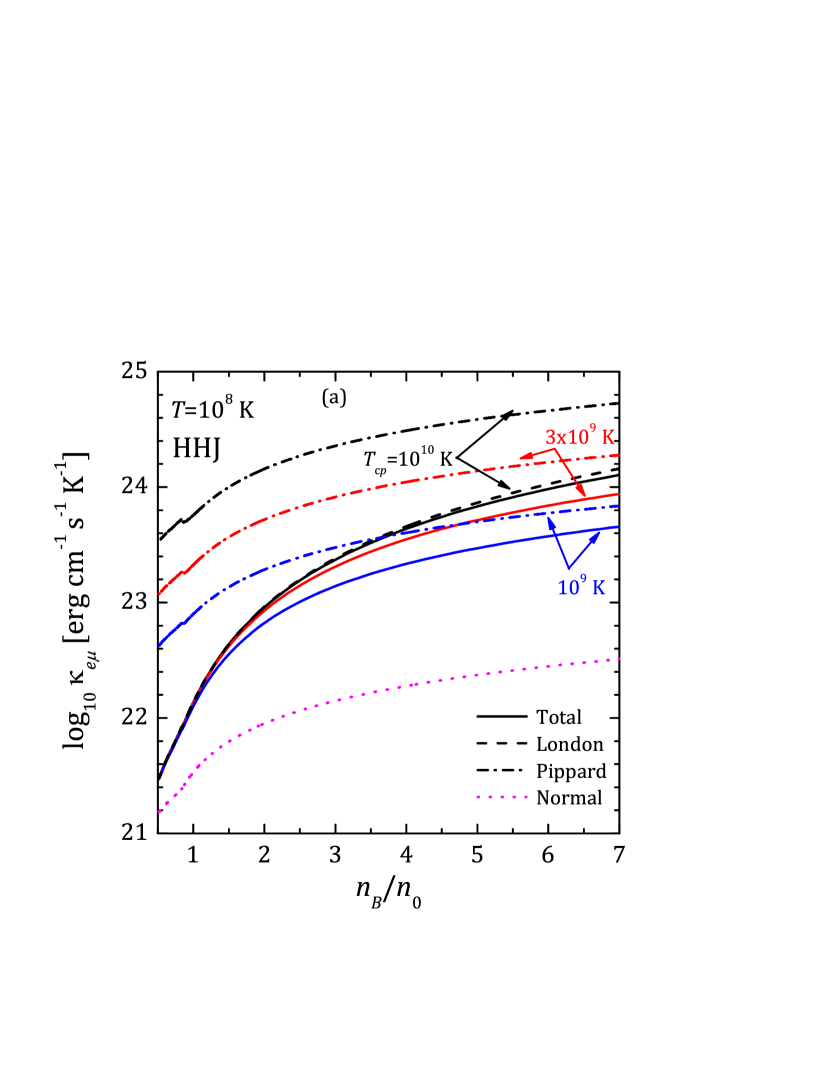
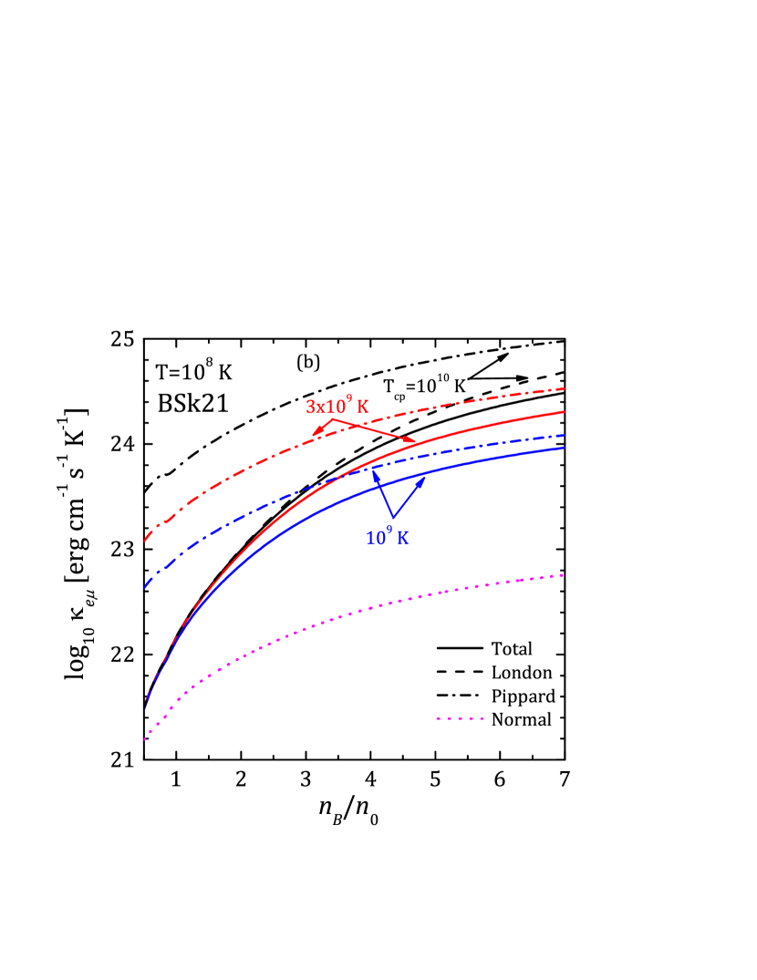
Figure 7: (Color online). Lepton thermal conductivity $\kappa_{e\mu}$ as a function of $n_{B}$ (a) for the HHJ EOS and (b) for the BSK21 EOS, $T=10^{8}$ K, and for three values of $T_{\mathrm{c}p}=10^{10}$, $3\times 10^{9}$, and $10^{9}$ K as indicated in the plot. Solid lines show the results of the present paper, dash-dotted lines correspond to the Pippard limit, and dashed lines to the London limit of transverse screening. Dotted lines show the calculations for normal (not superconducting) matter.

The results of the previous sections can be used for calculating the lepton contribution to transport coefficients of superconducting NS cores at not-too-high temperatures. Since these coefficients are governed by the electromagnetic interactions, the obtained results are applicable for any npe$\mu$ EOS of a neutron star core, provided the particle fractions and proton effective masses are known. It is clear from examining Eqs. (27)–(30), that the increase in proton fraction at a given baryon density lead to increase in both $\kappa_{e\mu}$ and $\eta_{e\mu}$. At the same time, the parameter $A$ increases with $x_{p}$ as well, so the crossover between the London and Pippard regimes occurs at lower $n_{B}$ for the EOS with higher proton fraction. Specifically, results are illustrated for two EOSs, HHJ and BSk21, and as before, the proton effective mass $m^{*}_{p}=0.8m_{u}$ is used. (The effect of effective mass variation is discussed separately below.) For completeness, all results discussed in this section employ exact solution of the system of transport equations taking into account all kinematical corrections as discussed in Secs. III.3–III.4.

Figure 7 shows the total lepton thermal conductivity $\kappa_{e\mu}$ as a function of $n_{B}$ for the HHJ EOS [panel (a)] and the BSk21 EOS [panel (b)], $T=10^{8}$ K and three values of $T_{\mathrm{c}p}=10^{10}$ K, $3\times 10^{9}$ K, and $10^{9}$ K. Remember, that the lepton thermal conductivity in a superconducting NS core scales as $\kappa_{e\mu}\propto T^{-1}$ as in the normal Fermi liquid. Solid lines give the results of the present paper with the corrected description of the transverse screening. Dash-dotted lines are calculated taking the screening in the Pippard limit, as in Ref. Shternin and Yakovlev (2007). According to Eq. (29), in this limit $\kappa_{e\mu}$ is approximately proportional to $\Delta$. Clearly, these results strongly overestimate $\kappa_{e\mu}$, especially at lower densities and higher values of $T_{\mathrm{c}p}$, which correspond to low values of the $A$ parameter. The dashed lines in Fig. 7 show $\kappa_{e\mu}$ calculated employing the transverse screening in the London limit. In this limit, $\kappa_{e\mu}$ is independent of $\Delta$, see Eq. (29), so only the single dashed line is present in Fig. 7. Thermal conductivity calculated in this limit also overestimates $\kappa_{e\mu}$. For low densities and/or high $T_{\mathrm{c}p}$, this overestimation is small. For instance, for $T_{\mathrm{c}p}=10^{10}$ K, dashed lines give rather good approximation for $\kappa_{e\mu}$ (compare with the solid lines) for all shown densities and for both EOSs. In contrast, for high densities and $T_{\mathrm{c}p}=10^{9}$ K, the Pippard limit gives much better approximation than the London one. Comparing left and right panels of Fig. 7, one can see that the difference between $\kappa_{e\mu}$ calculated in the Pippard limit and the correct value is smaller for the BSk21 EOS than for the HHJ EOS. Similarly, the difference between the London-limit calculations and exact ones (solid lines) is larger for the BSk21 EOS than for the HHJ EOS. This is a consequence of the larger value of the $A$ parameter for the BSk21 EOS (see Fig. 3). For comparison, with dotted lines in Fig. 7, $\kappa_{e\mu}^{N}$ calculated for the non-superconducting case is plotted. Again, all terms in the interaction are included, although the leading-order Eq. (15) gives a good approximation (notice, that correction to the variational solution is negligible in this case Shternin and Yakovlev (2007)). Since $\kappa_{e\mu}^{N}$ in leading order does not depend on temperature (see Sec. II), the difference between $\kappa_{e\mu}$ and $\kappa_{e\mu}^{N}$ increases with lowering $T$ Shternin and Yakovlev (2007). Taking this in mind and looking at the lower-density region in the left panel of Fig. 7 one can naively suggest that with increase of temperature, the normal-matter $\kappa_{e\mu}^{N}$ would become larger than $\kappa_{e\mu}$ for superconducting matter. This is not so, since in these conditions the assumption of the dominance of the proton contribution to the transverse screening will break down. In this case, one needs to include the dynamical contribution from the normal constituents of matter (leptons) to the transverse screening, see below. Presence of the normal matter contribution to screening effectively limits the collision frequencies from above, making them lower than in the normal case.

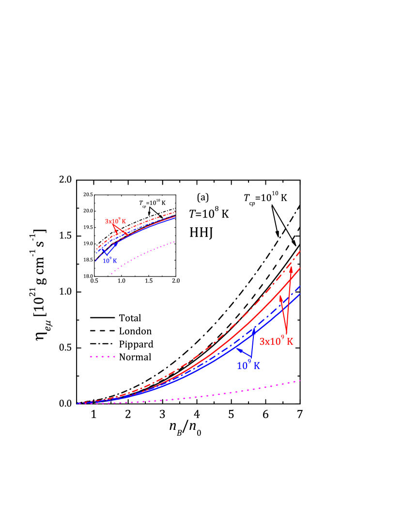
Figure 8: (Color online). Lepton shear viscosity (a) for the HHJ EOS and (b) for the BSK21 EOS as a function of $n_{B}$. The parameters of calculations and notations are the same as in Fig. 7. Notice, that the linear scale is used in this plot. Insets enlarge the region of $n_{B}$ up to $2n_{0}$, where the logarithmic scale for $\eta_{e\mu}$ is used.

Similar calculations for the shear viscosity $\eta_{e\mu}$ are shown in Fig. 8. Qualitatively, the situation is the same as for the thermal conductivity, although the differences between results in various approximations are less dramatic. This is a consequence of, first, the weaker dependence of the transverse collision frequencies $\nu^{\eta}_{ci}$ on the screening than found for $\nu^{\kappa}_{ci}$ and, second, of the larger contribution of the longitudinal part of the interaction to $\eta_{e\mu}$ than to $\kappa_{e\mu}$. For instance, the older results of Ref. Shternin and Yakovlev (2008) calculated in the Pippard limit (dash-dotted lines in Fig. 8) are acceptable for $T_{\mathrm{c}p}<3\times 10^{9}$ K, especially at higher densities. At most, the use of the Pippard limit results in an overestimation of $\eta_{e\mu}$ by a factor of 2.5 for $T=10^{9}$ K and lowest densities. This is not seen in Fig. 8 because of the linear scale, and is illustrated in the insets that show $\eta_{e\mu}$ up to $n_{B}=2n_{0}$ with the logarithmic scale. In the inset plots, due to a low density, the difference between $\eta_{e\mu}$ calculated for various $T_{\mathrm{c}p}$ and those calculated in London limit is barely seen. On the over hand, the overestimation that results from using the Pippard expression becomes visible. $\eta_{e\mu}^{N}$ calculated for non-superconducting matter is shown in Fig. 8 with dotted lines. Notice again, that the relation $\eta_{e\mu}^{N}\propto T^{-5/3}$ given by Eq. (16) works well only at low temperatures, where the transverse part of the interaction starts to dominate Shternin and Yakovlev (2008). Both the shear viscosity and the thermal conductivity for the BSk21 EOS are larger than those for the HHJ EOS. This is a consequence of different particle number fractions in these models.

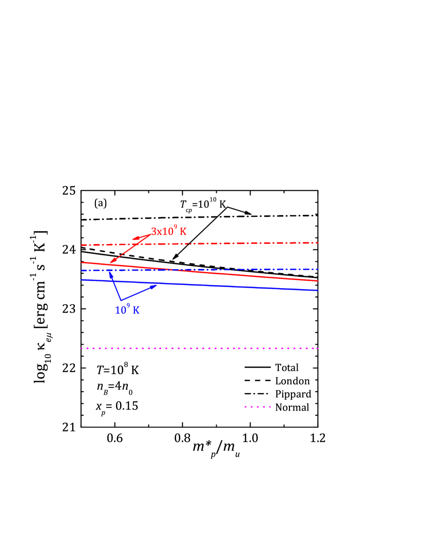
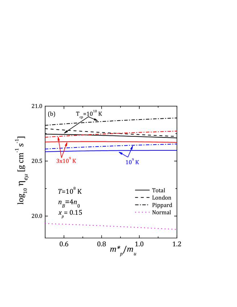
Figure 9: (Color online). Lepton thermal conductivity (a) and shear viscosity (b) calculated for $T=10^{8}$ K, $n_{B}=4n_{0}$, and proton fraction $x_{p}=0.15$ as functions of the proton effective mass $m^{*}_{p}$. The notations are the same as in Fig. 7.

In the previous discussion the constant (density-independent) proton effective mass was employed. It is instructive to look how the results depend on $m_{p}^{*}$. This is illustrated in Fig. 9 where the thermal conductivity [panel (a)] and shear viscosity [panel (b)] are plotted as a function of $m^{*}_{p}$ for the density $n_{B}=4n_{0}$ and proton fraction $x_{p}=0.15$. These are some typical values and do not correspond to a specific EOS. The line types and notations are similar to those in Figs. 7-8. Asymptotic expression in the Pippard limit in the leading order, Eqs. (29)–(30) do not depend on the proton effective mass. Some dependence on $m^{*}_{p}$ demonstrated by the dash-dotted lines in Fig. 9 is due to the corrections beyond the leading order. This dependence is more pronounced for the shear viscosity than for the thermal conductivity, in accordance with the discussion in Sec. III.3. Similar arguments apply for the transport coefficients of the normal matter shown with dotted lines in Fig. 9. In contrast, the asymptotic expressions in the London limit, Eqs. (27)–(28) explicitly depend on the proton effective mass through the Meissner momentum $q_{M}$. According to Eq. (19), an increase in $m^{*}_{p}$ leads to decrease in $q_{M}$ and hence to decrease of $\kappa_{e\mu}$ and $\eta_{e\mu}$. As seen in Fig. 9, this decrease is larger for $\kappa_{e\mu}$ than for $\eta_{e\mu}$ because of the weaker $q_{M}$-dependence of the latter, see Eqs. (27)–(28). The dependence of the results of the full calculations on the effective mass is in between the discussed limiting cases. Since the parameter $A$ decreases with $m_{p}^{*}$ [see Eq. (21)], London limiting expressions work better for larger $m_{p}^{*}$. Figure 9 shows that the use of the variable proton effective mass instead of the constant $m_{p}^{*}$ approximation can change the results illustrated in Figs. 7-8 quantitatively, but not qualitatively. In principle one should use the density dependence of $m_{p}^{*}$ consistent with the chosen EOS, but this is rarely provided.

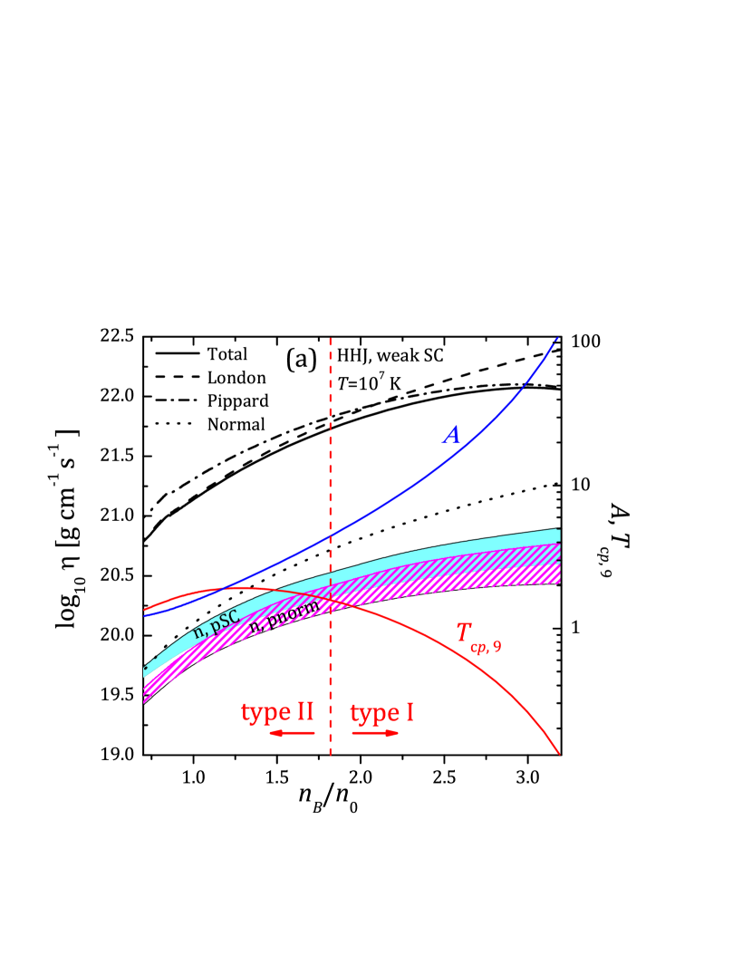
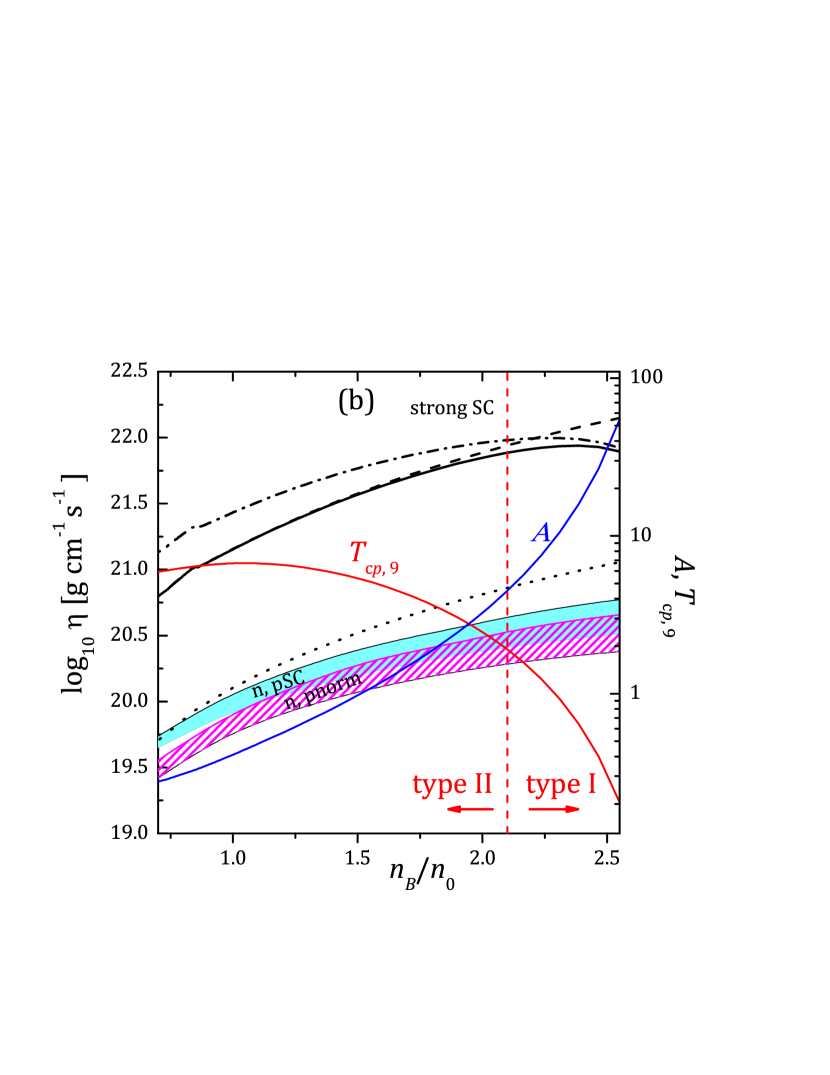
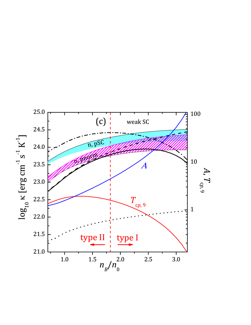
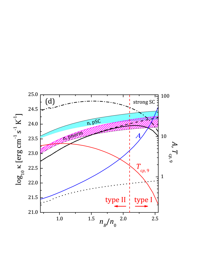
Figure 10: (Color online). Shear viscosity (a)–(b) and thermal conductivity (c)–(d) in the HHJ NS core for weak proton superconductivity model [panels (a) and (c)] and strong superconductivity model [panels (b) and (d)] discussed in the text. Temperature is set to $T=10^{7}$ K. As in previous figures, solid lines give full results of the present work, dash-dotted lines correspond to calculations in the Pippard limit, and dashed lines – to calculations in London limit. Dotted lines show the transports coefficients in normal matter. Lower hatched strips marked ‘n, pnorm’ and upper filled strips marked ‘n, pSC’ give the uncertainty bands for neutron transport coefficients in normal and superconducting matter, respectively. Thin solid lines and the right scales in each panel show the values of $T_{\mathrm{c}p,9}=T_{\mathrm{c}p}/10^{9}\leavevmode\nobreak\ {\rm K}$ and $A$ for each model. Vertical dashed lines ($A=\sqrt{2}\pi$) divide type-II and type-I superconductivity regions. See text for details

The proton critical temperature in the NS core is not constant but is actually density-dependent. It is instructive to illustrate the results by considering ‘realistic’ profiles $T_{\mathrm{c}p}(n_{B})$ in the NS core.This is done in Figs. 10 and 11 for the HHJ and the BSK21 EOSs, respectively. There exists a variety of calculations of the critical density profiles in a literature, each of which is based on a specific microscopic model. The results of these calculations generally do not agree with each other. In these circumstances it is instructive to rely on the phenomenological profiles $T_{\mathrm{c}p}(n_{B})$ instead of trying to handle EOS and superconductivity properties self-consistently Kaminker et al. (2001); Andersson et al. (2005). It is, however, reasonable to make these phenomenological models to resemble the extreme cases available on the market. Taking this in mind, following Glampedakis et al. (2011), I take two profiles of $T_{\mathrm{c}p}(n_{B})$ denoted by ‘e’ and ‘f’ in Ref. Andersson et al. (2005). These models are constructed by applying the phenomenological parametrization suggested by Kaminker et al. (2001) to the results of microscopic calculations of the proton ¹S₀ gaps Andersson et al. (2005). The critical temperature profiles for these models are shown in Fig. 10 for the HHJ EOS and in Fig. 11 for the BSk21 EOS with right vertical scales. The model ‘f’ describes weaker proton superconductivity based on the calculations in Ref. Amundsen and Østgaard (1985). The corresponding panels in Figs. 10 and 11 are marked ‘weak SC’. Panels (b) and (d) in the same Figs., marked ‘strong SC’, show results for stronger proton superconductivity model ‘e’ that is fitted to the results of Ref. Elgarøy et al. (1996), see Ref. Andersson et al. (2005) for details. With the same right vertical scale in each panel the corresponding density-dependence of the parameter $A$ is shown. Vertical dashed lines divide the regions of the superconductivity of the first and second types, according to the criterion $A>\sqrt{2}\pi$ ($\varkappa<1/\sqrt{2}$). Notice that the critical temperature profiles for the same superconductivity models are different for different EOSs because they actually depend on the proton Fermi momentum $p_{\mathrm{F}p}$ which differs in the HHJ and BSK21 EOSs at the same $n_{B}$.

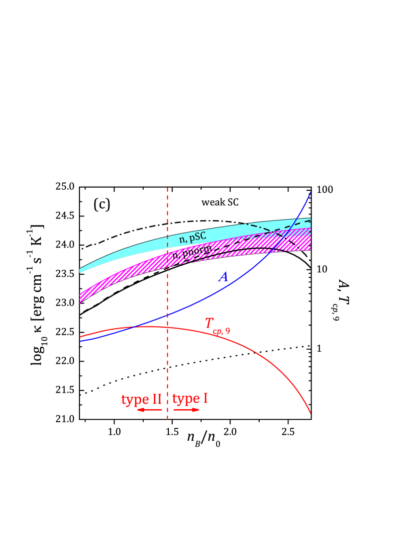
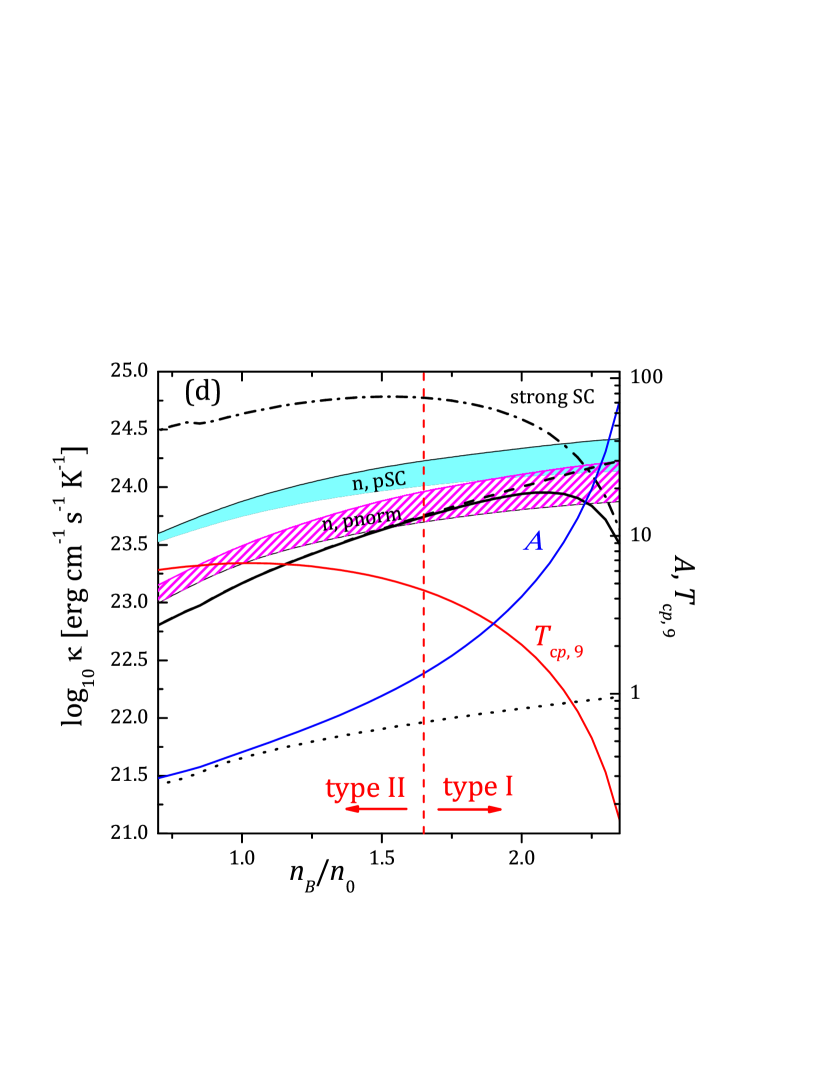
Figure 11: (Color online). Same as Fig. 10 but for the BSk21 EOS. Notations are the same as in Fig. 10.

The results for the shear viscosity $\eta_{e\mu}$ for the models ‘f’ and ‘e’ are shown in the panes (a) and (b), respectively, in Figs. 10 and 11. The thermal conductivity calculations are shown in panels (c) and (d) of the same figures. All calculations employ now $T=10^{7}$ K in order to meet the zero-temperature approximation in a whole density region shown (the low-temperature approximation can break down near the walls of the critical density profile, where $T_{\mathrm{c}p}$ is low). All the values can be scaled by $T^{2}$ for shear viscosity (by $T$ for thermal conductivity) provided the condition $T<0.35T_{\mathrm{c}p}$ is fulfilled in the density region of interest. As in Figs. 7–8, solid lines in Figs. 10–11 show the results of the full calculations, while dashed and dot-dashed lines are calculated in the London and Pippard limits, respectively. Dotted lines represent the lepton transport coefficients in normal matter. The results in Figs. 10–11 follow the same pattern as discussed above. The use of any of the limiting expressions, London or Pippard, for the transverse screening leads to an overestimation of the transport coefficients. The London limit is appropriate in the case of type-II superconductivity, while in the case of type-I superconductivity, the London limit is inappropriate and the Pippard limit can be a better approximation. In the intermediate case full calculations should be used. As seen from Figs. 10–11, in the real situation, both types of superconductivity can be simultaneously present in the NS cores Glampedakis et al. (2011).

For comparison, in Figs. 10–11 I also show the neutron shear viscosity $\eta_{n}$ and thermal conductivity $\kappa_{n}$ calculated following Refs. Shternin et al. (2013, 2017). In these Refs., the in-medium nucleon-nucleon interaction is treated in the Brueckner-Hartree-Fock framework with the inclusion of the effective three-body forces. The hatched strips in Figs. 10–11 show the results for normal (non-superconducting) beta-equilibrated matter, and the widths of the strips illustrate the uncertainty in calculations related to the different models of the nuclear interactions as considered in Ref. Shternin et al. (2017). The lower boundaries correspond to the nuclear interaction described by the Argonne v18 potential with addition of the three-body forces in the phenomenological Urbana IX model. Upper boundaries correspond to the same potential, but another model for the three-body interaction based on the meson-nucleon model of the nucleon interactions. More details can be found in Refs. Baldo et al. (2014); Shternin et al. (2017). Filled strips in Figs. 10–11 represent calculations of $\kappa_{n}$ and $\eta_{n}$ for the proton-superconducting matter. As in the case of the lepton transport coefficients, these results are obtained by neglecting the collisions with protons (they are damped exponentially in the considered limit). Then the neutron contribution to transport coefficients is mediated by the neutron-neutron collisions only. Notice, that the results for the neutron transport coefficients shown in Figs. 10–11 include the corrections to variational solution Shternin et al. (2013, 2017). Since $\kappa_{n}$ and $\eta_{n}$ are calculated within specific models of the nucleon interaction, the obtained results are not self-consistent with EOSs used elsewhere in the present paper. However, one expects that the results shown here give plausible estimates for the nucleon contribution (see Refs. Shternin et al. (2013) and Schmitt and Shternin (2017) for more discussion).

Since neutron-proton collisions are damped in the superconducting matter, respective $\kappa_{n}$ and $\eta_{n}$ values are larger than those in normal matter (see, e.g. Baiko et al. (2001); Shternin and Yakovlev (2008)). However this increase is much smaller than the increase in lepton transport coefficients, which are additionally boosted by the change of the screening behavior. According to Figs. 10–11, the relation between lepton and neutron transport coefficients remains qualitatively the same as in the non-superfluid matter. Namely, $\kappa_{n}>\kappa_{e\mu}$, while $\eta_{n}<\eta_{e\mu}$. Remember (Sec. II) that the neutron transport coefficients obey the standard Fermi-liquid behavior $\kappa_{n}\propto T^{-1}$, $\eta_{n}\propto T^{-2}$ as do the lepton transport coefficients in proton-superconducting matter.

All calculations above rely on the zero-temperature approximation $T/\Delta\lesssim 0.2$. In this limit, it is enough to use the expressions (18)–(20) for the proton part of the transverse screening. Since this screening is static, the lepton dynamical screening, which in the leading order is proportional to $\omega$, see Eq. (14), was neglected. In the Pippard limit this is possible when $\omega\ll\pi\Delta/r$, where $r=(p_{\mathrm{F}e}^{2}+p_{\mathrm{F}\mu}^{2})/p_{\mathrm{F}p}^{2}\approx 1$. Since typically $\omega\sim T$, this is always justified in our approximation. In the London limit, the similar comparison requires $\omega\sim T\ll 4/(3\pi)q_{M}v_{\mathrm{F}p}/r$. This requirement becomes stronger with lowering density, and transforms to $T\ll 10^{9}$ K for the BSk21 and HHJ EOSs at $n_{B}\approx 0.5n_{0}$.

When t emperature starts to increase, the superfluid density of protons $n_{sp}$ decreases and the Meissner momentum $q_{M}\propto n_{sp}^{1/2}$ also decreases. The screening becomes temperature-dependent. However, at low $q$ it is approximately constant, moreover the change of the screening behavior from the London one to the Pippard one occurs at the temperature-independent value $q\sim\xi_{0}^{-1}$, where $\xi_{0}\equiv\xi(T=0)$ Lifshitz and Pitaevskii (1980). Therefore, qualitatively, the results of the above analysis hold if one takes $A=\pi q_{M}(T)\xi_{0}$ (now $A$ is not related to $\varkappa$ which is independent of $T$). At a given density, $A$ decreases with increase of temperature making London limiting expressions more appropriate. Transport coefficients start to decrease, and in the leading order their temperature behavior is given by Eqs. (27)–(28), providing temperature-dependent $q_{M}(T)$ is used in this case. Such approach is possible until the dynamical part of the proton polarization function and the lepton contribution (14) start to be important. Thus, at the intermediate temperature the $\omega$ dependence of the transverse polarization function needs to be taken into account, that complicates the calculations Shternin and Yakovlev (2007, 2008). In the same region, the lepton-proton collisions start to be important that additionally decrease the transport coefficients. The consideration of the lepton-proton collisions is less straightforward since in the region of small momenta $qv_{\mathrm{F}p}\sim\Delta$ the renormalization of the proton current is necessary (e.g., Kundu and Reddy (2004); Arseev et al. (2006)). In addition, because of the gap in the proton spectrum, typical transferred energy is of the order of $\Delta$ and the limiting approximation $qv_{\mathrm{F}p}\gg\omega$ is not justified in the London limit. Fortunately, due to the exponential suppression of the lepton-proton collision frequencies, these effects need to be taken into account relatively close to the critical temperature where $\Delta(T)\sim T$. Then the approximation $qv_{\mathrm{F}p}\gg\omega$ is valid since $\omega\sim\Delta\sim T$. Clearly, the calculations of the transport coefficients in the transition region $0.35T_{\mathrm{c}p}\lesssim T\lesssim T_{\mathrm{c}p}$ are more involved than in the simple zero-temperature case. However, it seems sufficient in applications to construct the smooth interpolation between the results of the present paper at $T<0.35T_{\mathrm{c}p}$ and the normal matter results at $T>T_{\mathrm{c}p}$.

V Conclusions

I have calculated the electron and muon shear viscosity $\eta_{e\mu}$ and thermal conductivity $\kappa_{e\mu}$ in the proton-superconducting core of the NS based on the transport theory of the Fermi systems. The present results are applicable at the low temperatures, $T\lesssim 0.35T_{\mathrm{c}p}$, and differ from available calculations Shternin and Yakovlev (2007, 2008) by the corrected account of the screening of the electromagnetic interaction when the protons are in the paired state.

The variational results for the thermal conductivity and for the shear viscosity are obtained from Eqs. (1)–(2) using the appropriate collision frequencies. According to Secs. III.2–III.3, Eq. (23) with Eq. (53) can be used for thermal conductivity calculations. For the shear viscosity, it is enough to use the leading-order contributions in $q$ in Eqs. (35)–(38). The explicit expressions for these contributions are given by Eqs. (55)–(57). Finally, the simplest variational solution works well for $\eta_{e\mu}$, while for $\kappa_{e\mu}$ additional factor $C^{\kappa}=1.2$ should be used in Eq. (1) to correct the variational result.

The main conclusions of the present study are as follows:

1. In the superconducting NS cores, lepton transport coefficients obey the standard Fermi-liquid temperature dependence $\kappa_{e\mu}\propto T^{-1}$, $\eta_{e\mu}\propto T^{-2}$ in contrast to the situation in normal NS cores where $\kappa_{e\mu}\approx\mathrm{const}(T)$, $\eta_{e\mu}\propto T^{-5/3}$. This is a consequence of the static regime of the screening of electromagnetic interactions. The screening in the transverse channel is dominated by the proton contribution.

2. At a given density, $\kappa_{e\mu}$ and $\eta_{e\mu}$ increase with increase of the proton critical temperature $T_{\mathrm{c}p}$ (increase of the gap $\Delta$). At large densities, where the typical transferred momentum $q$ is large so that the Pippard limit for the transverse screening is applicable, one finds $\kappa_{e\mu}\propto\Delta$ and $\eta_{e\mu}\propto\Delta^{1/3}$. In the opposite limit of low densities, where the transverse electromagnetic interaction is screened by the Meissner momentum (the London limit), $\kappa_{e\mu}$ and $\eta_{e\mu}$ are independent of $\Delta$.

3. In general situation relevant for the NS cores, the whole range of momentum transfer is important, both limiting expressions overestimate transport coefficients, and the complete results developed here shall be used. However, in case of the superconductivity of the second kind it is enough to take the London limit for transverse screening and use corresponding limiting expressions for the transverse part of the collision frequencies. In case of the type-I superconductivity, the Pippard limit is more appropriate, although it is recommended to rely on the complete result in this limit.

4. Both limiting expressions can be used to estimate the transport coefficients from above. In this respect, the expression in London limit is more interesting since it gives the gap-independent boundary.

5. As in the case of the normal matter Shternin et al. (2013); Schmitt and Shternin (2017), leptons give dominant contribution to the shear viscosity while neutrons dominate the thermal conductivity.

Since the consideration of the lepton transport coefficients presented here does not rely of the specific EOS properties, the conclusions (i)–(iv) are universal in a sense that they are valid for any npe$\mu$ EOS of the dense matter in NS cores. In contrast, the conclusion (v) is model-dependent and need to be taken with caution. The neutron transport coefficients shown in Figs. 10–11 are calculated for different nucleon interactions, but within the single many-body approach, namely the Brueckner-Hartree-Fock scheme. Thus it is in principle not excluded that the conclusion (v) can fail for a specific microscopic model that produces significantly different values of $\kappa_{n}$ and $\eta_{n}$ than used here. Ideally, the neutron transport coefficients need to be calculated from the same microscopic model of the nucleon interaction as the EOS which is not a straightforward task. The detailed discussion of the neutron transport coefficients is outside the scope of the present paper, see Refs. Shternin et al. (2013); Schmitt and Shternin (2017) for more details.

The results obtained in the present paper can be improved by considering the finite temperature effects in order to study in detail the transition from the superconducting to the normal matter. This can be done following the same lines as described here, but considering the full temperature-dependent polarization functions. In this case, however, one needs to account for the dynamical part of the screening making the interaction $\omega$-dependent. In this case the integration over $\omega$ in Eqs. (3)–(II) cannot be performed analytically. Additional care must be taken when lepton collisions with the protonic excitations are considered. Anyway, it seems enough to interpolate through the transition region for practical applications, however the detailed investigation of the transition region remains to future studies.

In this paper I used polarization functions calculated in pure BCS framework, neglecting Fermi-liquid effects. In the Pippard limit this is a good approximation Gusakov (2010). However, the static screening in the London limit is affected Gusakov (2010). The consideration of these effects requires separate study. Moreover, it was proposed that the coupling between neutrons and protons in NS cores induces the effective electron-neutron interaction Bertoni et al. (2015) that modifies the screening properties of matter Stetina et al. (2018) and can affect the lepton collision frequencies. The effect of this interaction on the transport coefficients can be expected both in the normal and superconducting matter and is under investigation Stetina et al. (2018).

In the inner cores of NSs, hyperons can also appear Haensel et al. (2007). If they are normal (unpaired), the results of the present paper for lepton transport coefficients can be easily generalized by treating charged hyperons as passive scatterers. It is thought, however, that hyperons like the protons can be paired in the ${}^{1}S_{0}$ channel (since their number density is low), see e.g. review in Ref. Sedrakian and Clark (2018). In this case, their contribution to the transverse plasma screening should be considered in the same way as the proton one, although the situation will be more cumbersome since more than one gap is involved.

*

Appendix A Fitting expressions for integrals

The transverse integrals (22) can be normalized as

$$I_{n}=q_{M}^{3-n}\tilde{I}_{n}(x_{t},A),$$ (51)

where $x_{t}=q_{M}/q_{m}$ and

$$\tilde{I}_{n}(x_{t},A)=\int\limits_{0}^{1/x_{t}}\frac{x^{n}d\,x}{\left(x^{2}+J(Ax)\right)^{2}}.$$ (52)

The integrals $\tilde{I}_{n}(x_{t},A)$ were calculated on the dense grid and fitted by analytical expressions that take into account the correct asymptotic behavior in the limiting cases.

For $n=0$ the result is

$$\frac{p_{1}A^{1.5}+p_{2}A^{2}+\pi/4-x_{t}^{3}/3+p_{3}x_{t}^{4}+A\left(p_{4}-p_{5}x_{t}^{3}\right)}{1+p_{6}A},$$ (53)

where $p_{1}=0.0119$, $p_{2}=0.0063$, $p_{3}=0.202$, $p_{4}=0.108$, $p_{5}=0.454$, and $p_{6}=0.14$. Fit rms error is 0.4% and the maximal fitting error is 3% at $A=5$ and $x_{t}=0.76$.

Similarly, for $n=2$.

$$(1+p_{6}A)^{-1}\left[p_{1}A^{4/3}+\frac{\pi}{4}-x_{t}-p_{2}Ax_{t}+p_{3}x_{t}^{2}\right.$$

$$\left.+A^{2/3}(p_{4}+p_{5}x_{t})+A^{1/3}\left(p_{7}-p_{8}x_{t}+p_{9}x_{t}^{2}\right)\right],$$

(54)

where $p_{1}=0.094$, $p_{2}=0.234$, $p_{3}=0.356$, $p_{4}=0.1859$, $p_{5}=0.0496$, $p_{6}=0.227$, $p_{7}=-0.0537$, $p_{8}=-0.2345$, and $p_{9}=0.239$. Fit rms error is $\sim 1$% and the maximal fitting error is 7% at $A=0.5$ and $x_{t}=0.14$.

The leading-order contributions to the collision frequencies relevant for the shear viscosity problem (36)–(38) can be given as

$$\nu^{\eta,t}_{ci}=\frac{2\pi\alpha_{f}^{2}T^{2}p_{\mathrm{F}i}^{2}}{m_{c}^{*}p_{\mathrm{F}c}}I^{t}_{2},$$ (55)

$$\nu^{\eta,l}_{ci}=\frac{2\pi\alpha_{f}^{2}T^{2}m_{c}^{*}m_{i}^{*2}}{p_{\mathrm{F}c}^{3}q_{\mathrm{TF}}}\left(\mathrm{arctan}\frac{q_{m}}{q_{\mathrm{TF}}}+\frac{q_{\mathrm{TF}}q_{m}}{q_{\mathrm{TF}}^{2}+q_{m}^{2}}\right),$$ (56)

$${\nu^{\prime}}^{\eta}_{ci}=\frac{4\pi\alpha_{f}^{2}T^{2}m_{i}^{*}p_{\mathrm{F}i}}{p_{\mathrm{F}c}^{2}q_{\mathrm{TF}}}\mathrm{arctan}\frac{q_{m}}{q_{\mathrm{TF}}}.$$ (57)