Fiducial distributions in Higgs and Drell-Yan production at N³LL+NNLO

Abstract

The perturbative description of certain differential distributions across a wide kinematic range requires the matching of fixed-order perturbation theory with resummation of large logarithmic corrections to all orders. We present precise matched predictions for transverse-momentum distributions in Higgs boson (H) and Drell-Yan pair (DY) production as well as for the closely related $\phi^{*}_{\eta}$ distribution at the LHC. The calculation is exclusive in the Born kinematics, and allows for arbitrary fiducial selection cuts on the decay products of the colour singlets, which is of primary relevance for experimental analyses. Our predictions feature very small residual scale uncertainties and display a good convergence of the perturbative series. A comparison of the predictions for DY observables to experimental data at $8~{}\mathrm{TeV}$ shows a very good agreement within the quoted errors.

1 Introduction

The accurate prediction and measurement of differential distributions is of primary importance for the LHC precision programme, especially in view of the absence of clear signals of new physics in the data collected so far. In this context, a special role is played by the kinematic distributions of a colour singlet produced in association with QCD radiation. These observables are often measured by reconstructing the decay products of the colour singlet (whenever possible), which are sensitive to the accompanying hadronic activity only through kinematic recoil. As a consequence, measurements of transverse and angular observables often lead to small experimental systematic uncertainties Khachatryan:2016nbe ; Aaij:2016mgv ; Aaboud:2017soa ; Aaboud:2017oem ; Sirunyan:2017igm ; Sirunyan:2017exp ; Aaboud:2018xdt ; Sirunyan:2018ouh .

The implication of these precise measurements is twofold. On one hand, they can be used to fit the parameters of the SM Lagrangian (e.g. strong coupling constant, or masses) or to calibrate the models that typically enter the calculation of hadron-collider observables (like for instance collinear parton distribution functions (PDFs) Ball:2017nwa , or non-perturbative corrections and transverse-momentum-dependent PDFs Scimemi:2016ffw ; Scimemi:2017etj ; Bacchetta:2017gcc ). An example is given by the differential distributions in $Z$- and $W$-boson production, that recently were exploited to perform very precise extractions of the $W$-boson mass Aaboud:2017svj and to constrain the behaviour of some PDFs Boughezal:2017nla . On the other hand, an excellent control over kinematic distributions is a way to set compelling constraints on new-physics models that would lead to mild shape distortions. An example is given by the sensitivity of the Higgs transverse-momentum ($p_{t}$) distribution to modification of the Yukawa couplings of the Higgs to quarks Bishara:2016jga ; Soreq:2016rae .

In this article we present state-of-the-art predictions for a class of differential distributions both in Higgs boson (H) and Drell-Yan pair (DY) production. Specifically, we combine fixed-order calculations at next-to-next-to-leading order (NNLO) with the recently-obtained resummation of Sudakov logarithms to next-to-next-to-next-to-leading-logarithmic order (N³LL), for the transverse-momentum spectrum of the colour singlet, as well as for the angular variable $\phi^{*}_{\eta}$ Banfi:2010cf . In the following, for simplicity, we will collectively denote $p_{t}/M$ or $\phi^{*}_{\eta}$ by $v$, with $M$ representing the invariant mass of the colour singlet.

Inclusive and differential distributions for Higgs-boson production in gluon fusion are nowadays known with very high precision. The inclusive cross section has been computed to next-to-next-to-next-to-leading-order (N³LO) accuracy in QCD deFlorian:1999zd ; Harlander:2002wh ; Anastasiou:2002yz ; Ravindran:2003um ; Ravindran:2002dc ; Anastasiou:2016cez ; Mistlberger:2018etf in the heavy-top-quark limit. The impact of all-order effects due to a combined resummation of threshold and high-energy logarithms has been studied in detail, and at the current collider energies the corrections amount to a few-percent of the total cross section Bonvini:2018ixe , indicating that the missing higher-order contributions are under good theoretical control. The state-of-the-art results for the Higgs transverse-momentum spectrum in fixed-order perturbation theory are the next-to-next-to-leading-order (NNLO) computations of Refs. Boughezal:2015dra ; Boughezal:2015aha ; Caola:2015wna ; Chen:2016zka , which have been obtained in the heavy-top-quark limit. The effect of finite quark masses on differential distributions at next-to-leading order has been recently computed in Refs. Melnikov:2017pgf ; Lindert:2017pky ; Lindert:2018iug ; Neumann:2018bsx ; Caola:2018zye ; Jones:2018hbb .

The state-of-the-art for the QCD corrections to differential distributions in DY production is at a similar level of accuracy. The total cross section is known fully differentially in the Born phase space up to NNLO Hamberg:1990np ; vanNeerven:1991gh ; Anastasiou:2003yy ; Melnikov:2006di ; Melnikov:2006kv ; Catani:2010en ; Catani:2009sm ; Gavin:2010az ; Anastasiou:2003ds , while differential distributions in transverse momentum were recently computed up to NNLO both for $Z$- Ridder:2015dxa ; Ridder:2016nkl ; Gehrmann-DeRidder:2016jns ; Gauld:2017tww ; Boughezal:2015ded ; Boughezal:2016isb and $W$-boson Boughezal:2015dva ; Boughezal:2016dtm ; Gehrmann-DeRidder:2017mvr production. In the DY distributions, electroweak corrections become important especially at large transverse momenta, and they have been computed to NLO in Kuhn:2005az ; Kuhn:2007qc ; Denner:2009gj ; Denner:2011vu .

Although fixed-order results are crucial to obtain reliable theoretical predictions away from the soft and collinear regions of the phase space ($v\sim 1$), it is well known that regions dominated by soft and collinear QCD radiation—which give rise to the bulk of the total cross section—are affected by large logarithmic terms of the form $\alpha_{\mathrm{s}}^{n}\ln^{k}(1/v)/v$, with $k\leq 2n-1$, which spoil the convergence of the perturbative series at small $v$. In order to have a finite and well-behaved calculation in this limit, the subtraction of the infrared and collinear divergences requires an all-order resummation of the logarithmically divergent terms. The logarithmic accuracy is commonly defined in terms of the perturbative series of the logarithm of the cumulative cross section $\Sigma$ as

$$\ln\Sigma(v) \equiv\ln\int_{0}^{v}\mathrm{d}v^{\prime}\;\frac{\mathrm{d}\Sigma(v^{\prime})}{\mathrm{d}v^{\prime}}$$

$$=\sum_{n}\left\{{\cal O}\left(\alpha_{\mathrm{s}}^{n}\ln^{n+1}(1/v)\right)+{\cal O}\left(\alpha_{\mathrm{s}}^{n}\ln^{n}(1/v)\right)+{\cal O}\left(\alpha_{\mathrm{s}}^{n}\ln^{n-1}(1/v)\right)+\dots\right\}.$$ (1)

One refers to the dominant terms $\alpha_{\mathrm{s}}^{n}\ln^{n+1}(1/v)$ as leading logarithmic (LL), to terms $\alpha_{\mathrm{s}}^{n}\ln^{n}(1/v)$ as next-to-leading logarithmic (NLL), to $\alpha_{\mathrm{s}}^{n}\ln^{n-1}(1/v)$ as next-to-next-to-leading logarithmic (NNLL), and so on.

The resummation of the $p_{t}$ spectrum of a heavy colour singlet is commonly performed in impact-parameter ($b$) space Parisi:1979se ; Collins:1984kg , where the observable completely factorises and the resummed cross section takes an exponential form. Using the $b$-space formulation the Higgs $p_{t}$ spectrum was resummed at NNLL accuracy in Refs. Bozzi:2005wk ; deFlorian:2012mx ; Becher:2012yn , following either the conventional approach of Ref. Collins:1984kg , or a soft-collinear-effective-theory Bauer:2000ew ; Bauer:2000yr ; Bauer:2001yt ; Bauer:2002nz (SCET) formulation of Refs. Becher:2010tm ; GarciaEchevarria:2011rb . A study of the related theory uncertainties in the SCET formulation was presented in Ref. Neill:2015roa . In DY production, NNLL predictions for the transverse momentum of the color singlet as well as for $\phi^{*}_{\eta}$ were obtained in Refs. Bozzi:2010xn ; Becher:2010tm ; Banfi:2012du . The impact of both threshold and high-energy resummation on the small-transverse-momentum region was also studied in detail in Refs. Li:1998is ; Laenen:2000ij ; Kulesza:2003wn ; Marzani:2015oyb ; Forte:2015gve ; Caola:2016upw ; Lustermans:2016nvk ; Marzani:2016smx ; Muselli:2017bad and the effects were found to be quite moderate at LHC energies.

The problem of the resummation of the transverse-momentum distribution in direct ($p_{t}$) space received substantial attention throughout the years Ellis:1997ii ; Frixione:1998dw ; Kulesza:1999sg , but remained unsolved until recently. Due to the vectorial nature of $p_{t}$ (analogous considerations apply to $\phi^{*}_{\eta}$), it is indeed not possible to define a resummed cross section at a given logarithmic accuracy in direct space that is simultaneously free of both subleading-logarithmic contributions and spurious singularities at finite, non-zero values of $p_{t}$. A possible solution to the problem was recently proposed in Refs. Monni:2016ktx ; Bizon:2017rah , in whose formalism the resummation is performed by generating the relevant QCD radiation by means of a Monte Carlo (MC) algorithm. The resummation of the $p_{t}$ spectrum in momentum space has been also studied in Ref. Ebert:2016gcn within a SCET framework, where the renormalisation-group evolution is performed directly in $p_{t}$ space. An alternative technique to analytically transform the impact-parameter-space result into momentum space was recently proposed in Ref. Kang:2017cjk .

All the necessary ingredients for the N³LL resummation of $p_{t}$ (and $\phi^{*}_{\eta}$) spectra in color-singlet production have been computed in Catani:2011kr ; Catani:2012qa ; Gehrmann:2014yya ; Echevarria:2016scs ; Li:2016ctv ; Vladimirov:2016dll , and the four-loop cusp anomalous dimension has been recently obtained numerically in refs. Moch:2017uml ; Moch:2018wjh . This has paved the way to more accurate theoretical results for transverse observables in the infrared region, like for instance the computation of the Higgs-transverse-momentum spectrum at N³LL matched to NNLO in Refs. Bizon:2017rah ; Chen:2018pzu . In this manuscript, employing the direct-space resummation at N³LL accuracy of Ref. Bizon:2017rah matched to NNLO, we present results for Higgs $p_{t}$ both at the inclusive level and with fiducial cuts on the decay products in the $H\to\gamma\gamma$ channel. We also consider Drell-Yan pair production and compute N³LL+NNLO predictions for the transverse momentum of the lepton pair and for the $\phi^{*}_{\eta}$ observable, comparing these results to ATLAS measurements at $8~{}\mathrm{TeV}$.

The article is organised as follows. In section 2 we discuss the computation of the NNLO differential distributions in DY and H production with the fixed-order parton-level code NNLOjet. Section 3 contains a brief review of the resummation for the $p_{t}$ and $\phi^{*}_{\eta}$ distributions using a momentum-space approach as implemented in the computer code RadISH, and in section 4 we discuss in detail the matching to fixed order together with the validation of our calculation. Section 5 reports the results for H production, while the analogous results for DY production are reported in Section 6. Section 7 contains our conclusions. We report the relevant formulae used for the matching in Appendix A, while Appendix B contains various quantities necessary for the resummation up to N³LL.

2 Fixed order

In this article we consider the production of either a Higgs boson or a leptonic Drell-Yan pair. In particular, the main focus lies in the description of the transverse-momentum spectrum and, in the case of DY production, of the closely related $\phi^{*}_{\eta}$ observable. These observables are studied in the context of matching the fixed-order calculation to a resummed prediction, and consequently the low- to intermediate-$p_{t}$ regimes are of particular interest.

For the Higgs production process, we therefore restrict ourselves to the region with $p_{t}^{\rm H}\lesssim m_{t}$ where the HEFT description is appropriate. In this effective-field-theory framework, the top quark is integrated out in the large-top-mass limit ($m_{t}\rightarrow\infty$), giving rise to an effective operator that directly couples the Higgs field to the gluon field-strength tensor via Wilczek:1977zn ; Shifman:1978zn ; Inami:1982xt

$$\mathcal{L}_{\text{HEFT}}=-\frac{\lambda}{4}\;G^{\mu\nu}G_{\mu\nu}H.$$ (2)

The Wilson coefficient $\lambda$ is known to three-loop accuracy Chetyrkin:1997un and its renormalisation-scale dependence was studied in Chen:2016zka . We consider the $p_{t}^{\rm H}$ spectrum for both the inclusive production of an on-shell Higgs boson as well as including its decay into two photons. For the latter, the production and decay are treated in the narrow-width approximation and fiducial cuts, summarised in Section 5, are applied on the photons in the final state.

For the DY process, we consider the full off-shell production of a charged lepton pair, including both the $Z$-boson and photon exchange contributions. Fiducial cuts are applied to the leptons in the final state and match the corresponding measurement performed by ATLAS at $8~{}\mathrm{TeV}$ Aad:2015auj , which are summarised in Section 6. We consider both the $p_{t}^{\rm Z}$ spectrum as well as the $\phi^{*}_{\eta}$ distribution, which are further studied multi-differentially for different invariant-mass ($M_{\ell\ell}$) or rapidity ($Y_{\ell\ell}$) bins.

The differential distributions in $v=p_{t}/M,~{}\phi^{*}_{\eta}$ for the production of a colour singlet at hadron colliders are indirectly generated through the recoil of the colour singlet against QCD radiation. The observables $v$ are therefore closely related to the $X+\text{jet}$ process with $X=H,~{}Z$, where the jet requirement is replaced by a restriction on $v$ to be non-vanishing: $v\geq v_{\text{cut}}>0$. The state-of-the-art fixed-order QCD predictions for this class of processes is at NNLO Boughezal:2015dra ; Boughezal:2015aha ; Caola:2015wna ; Chen:2016zka ; Ridder:2015dxa ; Ridder:2016nkl ; Gehrmann-DeRidder:2016jns ; Gauld:2017tww ; Boughezal:2015ded ; Boughezal:2016isb . Starting from the LO distributions, in which the colour singlet recoils against a single parton, the NNLO predictions receive contributions from configurations (with respect to LO) with two extra partons (RR: double-real corrections for H DelDuca:2004wt ; Dixon:2004za ; Badger:2004ty and DY Campbell:2002tg ; Campbell:2003hd ; Hagiwara:1988pp ; Berends:1988yn ; Falck:1989uz ), with one extra parton and one extra loop (RV: real-virtual corrections for H Dixon:2009uk ; Badger:2009hw ; Badger:2009vh and DY Campbell:2002tg ; Campbell:2003hd ; Glover:1996eh ; Bern:1996ka ; Campbell:1997tv ; Bern:1997sc ) and with no extra parton but two extra loops (VV: double-virtual corrections for H Gehrmann:2011aa and DY Moch:2002hm ; Garland:2001tf ; Garland:2002ak ; Gehrmann:2011ab ). Each of the three contributions is separately infrared divergent either in an implicit manner from phase-space regions where parton radiations become unresolved (soft and/or collinear) or in a explicit manner from divergent poles in virtual loop corrections. Only the sum of the three contributions is finite.

Our calculation is performed using the parton-level event generator NNLOjet, which implements the antenna subtraction method GehrmannDeRidder:2005hi ; Daleo:2006xa ; Currie:2013vh to isolate infrared singularities and to enable their cancellation between different contributions prior to the numerical phase-space integration. The NNLO corrections for Higgs and DY production at finite $v$ are calculated using established implementations for $pp\rightarrow H+\text{jet}$ Chen:2014gva ; Chen:2016zka and $pp\rightarrow Z+\text{jet}$ Ridder:2015dxa ; Ridder:2016nkl ; Gehrmann-DeRidder:2016jns ; Gauld:2017tww at NNLO, and it takes the schematic form:

$$\sigma^{\text{NNLO}}_{X+\text{jet}}= \int_{\Phi_{X+3}}\Big{(}\mathrm{d}\sigma^{RR}_{\text{NNLO}}-\mathrm{d}\sigma^{S}_{\text{NNLO}}\Big{)}$$

$$+ \int_{\Phi_{X+2}}\Big{(}\mathrm{d}\sigma^{RV}_{\text{NNLO}}-\mathrm{d}\sigma^{T}_{\text{NNLO}}\Big{)}$$

$$+ \int_{\Phi_{X+1}}\Big{(}\mathrm{d}\sigma^{VV}_{\text{NNLO}}-\mathrm{d}\sigma^{U}_{\text{NNLO}}\Big{)}.$$ (3)

The antenna subtraction terms, $\mathrm{d}\sigma^{S,T,U}_{\text{NNLO}}$, for both Higgs and Drell-Yan related processes are constructed from antenna functions GehrmannDeRidder:2005cm ; GehrmannDeRidder:2005aw ; Daleo:2009yj ; Boughezal:2010mc ; Gehrmann:2011wi ; GehrmannDeRidder:2012ja to cancel infrared singularities between the contributions of different parton multiplicities. The integrals are performed over the phase space ${\Phi_{X+1,2,3}}$ corresponding to the production of the colour singlet in association with one, two or three partons in the final state. The integration of the final-state phase space is fully differential such that any infrared-safe observable $\cal O$ can be studied through differential distributions as $\mathrm{d}\sigma^{\text{NNLO}}_{X+\text{jet}}/\mathrm{d}\cal O$.

For large values of $v$ ($v\sim 1$), the phase-space integral in each line of Eq. (2) is well defined and was calculated with high numerical precision in previous studies. Extending these predictions to smaller, but finite $v\ (\sim 0.01)$ becomes extremely challenging due to the wider dynamical range that is probed in the integration. Both the matrix elements and the subtraction terms grow rapidly in magnitude towards smaller values of $v$, thereby resulting in large numerical cancellations between them and rendering both the numerical precision and the stability of the results challenging. The finite remainder of such cancellations needs to be numerically stable in order to be consistently combined with resummed logarithmic corrections and extrapolated to the limit $v\to 0$. For this reason, the integration is performed separately for each individual initial-state partonic channel. We further split the integration region for each channel into multiple intervals in $v$, which are partially overlapping with each other. By carefully checking the consistency of the distributions in the overlapping region and using dedicated reweighting factors in each interval, we use NNLOjet to produce fixed-order predictions up to NNLO for values in $v$ down to $p_{t}=2~{}\mathrm{GeV}$ and $\phi^{*}_{\eta}=0.004$ Gehrmann-DeRidder:2016jns .

The accuracy of the results obtained with the NNLOjet code for small $v$ has been systematically validated in Ref. Chen:2018pzu by comparing fixed-order predictions of the Higgs boson transverse momentum distribution $\mathrm{d}\sigma_{\text{NNLO}}/\mathrm{d}p_{t}^{\rm H}$ against the expansion of the N³LL resummation (obtained in the framework of soft-collinear effective field theory, SCET) to the respective order in the small $p_{t}^{\rm H}$ region. This validation was performed for individual initial-state partonic channels down to $p_{t}^{\rm H}=0.7~{}\mathrm{GeV}$.

As $v\rightarrow 0$, the final-state phase space $\Phi_{X+1,2,3}$ is reduced to the phase space of colour singlet production $\Phi_{X}$. The RR, RV, and VV contributions contain infrared divergences with one extra unresolved parton that cannot be cancelled by the subtraction terms $\mathrm{d}\sigma^{S,T,U}_{\text{NNLO}}$. These extra logarithmic divergences are cancelled by combining the fixed-order computation to a resummed calculation, where the logarithms in the fixed-order prediction are subtracted and replaced by a summation of the corresponding enhanced terms to all orders in perturbation theory. This operation is discussed in the next section, and more details on the combination of the two results are reported in Appendix A.

3 Resummation

The approach developed in Refs. Monni:2016ktx ; Bizon:2017rah uses the factorisation properties of the QCD squared amplitudes to devise a Monte Carlo formulation of the all-order calculation. In this framework, large logarithms are resummed directly in momentum space by effectively generating soft and/or collinear emissions in a fashion similar in spirit to an event generator.

To summarise the final result, we consider the cumulative distribution

$$\Sigma(v)\equiv\int_{0}^{v}\mathrm{d}v^{\prime}\;\frac{\mathrm{d}\Sigma(v^{\prime})}{\mathrm{d}v^{\prime}}$$ (4)

for an observable $v^{(\prime)}=V(\Phi_{B},k_{1},\dots,k_{n})$, being either $p_{t}/M$ or $\phi^{*}_{\eta}$, in the presence of $n$ real emissions with momenta $k_{1},...,k_{n}$. Using the notation of Ref. Bizon:2017rah , $\Sigma(v)$ can be expressed as

$$\Sigma(v)=\int\mathrm{d}\Phi_{B}{\cal V}(\Phi_{B})\sum_{n=0}^{\infty}\int\prod_{i=1}^{n}[\mathrm{d}k_{i}]|{\cal M}(\Phi_{B},k_{1},\dots,k_{n})|^{2}\,\Theta\left(v-V(\Phi_{B},k_{1},\dots,k_{n})\right)\,,$$ (5)

where ${\cal M}$ is the matrix element for $n$ real emissions and ${\cal V}(\Phi_{B})$ denotes the resummed form factor that encodes the purely virtual corrections Dixon:2008gr . The phase spaces of the $i$-th emission $k_{i}$ and that of the Born configuration are denoted by $[\mathrm{d}k_{i}]$ and $\mathrm{d}\Phi_{B}$, respectively.

The recursive infrared and collinear (rIRC) safety Banfi:2004yd of the observable allows one to establish a well defined logarithmic counting in the squared amplitude Banfi:2004yd ; Banfi:2014sua , and to systematically identify the contributions that enter at a given logarithmic order. In particular, the squared amplitude can be decomposed in terms of $n$-particle-correlated blocks, such that blocks with $n$ particles start contributing one logarithmic order higher than blocks with $n-1$ particles.

Eq. (5) contains exponentiated divergences of virtual origin in the $\mathcal{V}(\Phi_{B})$ factor, as well as singularities in the real matrix elements, which appear at all perturbative orders. In order to handle such divergences, one can introduce a resolution scale $Q_{0}$ on the transverse momentum of the radiation: thanks to rIRC safety, unresolved real radiation (i.e. softer than $Q_{0}$) does not contribute to the observable’s value, namely it can be neglected when computing $V(\Phi_{B},k_{1},\dots,k_{n})$, thus it exponentiates and cancels the divergences contained in $\mathcal{V}(\Phi_{B})$ at all orders. The precise definition of the unresolved radiation requires a careful clustering of momenta belonging to a given correlated block in order to be collinear safe. On the other hand, the real radiation harder than the resolution scale (referred to as resolved) must be generated exclusively since it is constrained by the $\Theta$ function in Eq. (5). rIRC safety also ensures that the dependence of the results upon $Q_{0}$ is power-like, hence the limit $Q_{0}\to 0$ can be taken safely.

For observables which depend on the total transverse momentum of QCD radiation, such as $p_{t}$ or $\phi^{*}_{\eta}$, it is particularly convenient to set the resolution scale to a small fraction $\delta>0$ of the transverse momentum of the block with largest $k_{t}$, hereby denoted by $\delta k_{t1}$, which allows for an efficient Monte Carlo implementation of the resulting resummed formula that can be used to simultaneously compute both $p_{t}$ and $\phi^{*}_{\eta}$.

Including terms up to N³LL, the cumulative cross section in momentum space can be recast in the following form Bizon:2017rah

$$\frac{\mathrm{d}\Sigma(v)}{\mathrm{d}\Phi_{B}}=\int_{0}^{\infty}\frac{\mathrm{d}k_{t1}}{k_{t1}}{\cal J}(k_{t1})\frac{\mathrm{d}\phi_{1}}{2\pi}\partial_{\tilde{L}}\left(-\mathrm{e}^{-\tilde{R}(k_{t1})}{\tilde{\cal L}}_{\rm N^{3}LL}(k_{t1})\right)\int\mathrm{d}\mathcal{Z}[\{{\tilde{R}}^{\prime},k_{i}\}]\Theta\left(v-V(\Phi_{B},k_{1},\dots,k_{n+1})\right)$$

$$+\int_{0}^{\infty}\frac{\mathrm{d}k_{t1}}{k_{t1}}{\cal J}(k_{t1})\frac{\mathrm{d}\phi_{1}}{2\pi}\mathrm{e}^{-\tilde{R}(k_{t1})}\int\mathrm{d}\mathcal{Z}[\{{\tilde{R}}^{\prime},k_{i}\}]\int_{0}^{1}\frac{\mathrm{d}\zeta_{s}}{\zeta_{s}}\frac{\mathrm{d}\phi_{s}}{2\pi}\Bigg{\{}\bigg{(}{\tilde{R}}^{\prime}(k_{t1}){\tilde{\cal L}}_{\rm NNLL}(k_{t1})-\partial_{\tilde{L}}{\tilde{\cal L}}_{\rm NNLL}(k_{t1})\bigg{)}$$

$$\times\left({\tilde{R}}^{\prime\prime}(k_{t1})\ln\frac{1}{\zeta_{s}}+\frac{1}{2}{\tilde{R}}^{\prime\prime\prime}(k_{t1})\ln^{2}\frac{1}{\zeta_{s}}\right)-{\tilde{R}}^{\prime}(k_{t1})\left(\partial_{\tilde{L}}{\tilde{\cal L}}_{\rm NNLL}(k_{t1})-2\frac{\beta_{0}}{\pi}\alpha_{\mathrm{s}}^{2}(k_{t1})\hat{P}^{(0)}\otimes{\tilde{\cal L}}_{\rm NLL}(k_{t1})\ln\frac{1}{\zeta_{s}}\right)$$

$$+\frac{\alpha_{\mathrm{s}}^{2}(k_{t1})}{\pi^{2}}\hat{P}^{(0)}\otimes\hat{P}^{(0)}\otimes{\tilde{\cal L}}_{\rm NLL}(k_{t1})\Bigg{\}}\bigg{\{}\Theta\left(v-V(\Phi_{B},k_{1},\dots,k_{n+1},k_{s})\right)-\Theta\left(v-V(\Phi_{B},k_{1},\dots,k_{n+1})\right)\bigg{\}}$$

$$+\frac{1}{2}\int_{0}^{\infty}\frac{\mathrm{d}k_{t1}}{k_{t1}}{\cal J}(k_{t1})\frac{\mathrm{d}\phi_{1}}{2\pi}\mathrm{e}^{-\tilde{R}(k_{t1})}\int\mathrm{d}\mathcal{Z}[\{{\tilde{R}}^{\prime},k_{i}\}]\int_{0}^{1}\frac{\mathrm{d}\zeta_{s1}}{\zeta_{s1}}\frac{\mathrm{d}\phi_{s1}}{2\pi}\int_{0}^{1}\frac{\mathrm{d}\zeta_{s2}}{\zeta_{s2}}\frac{\mathrm{d}\phi_{s2}}{2\pi}{\tilde{R}}^{\prime}(k_{t1})$$

$$\times\Bigg{\{}{\tilde{\cal L}}_{\rm NLL}(k_{t1})\left({\tilde{R}}^{\prime\prime}(k_{t1})\right)^{2}\ln\frac{1}{\zeta_{s1}}\ln\frac{1}{\zeta_{s2}}-\partial_{\tilde{L}}{\tilde{\cal L}}_{\rm NLL}(k_{t1}){\tilde{R}}^{\prime\prime}(k_{t1})\bigg{(}\ln\frac{1}{\zeta_{s1}}+\ln\frac{1}{\zeta_{s2}}\bigg{)}$$

$$+\frac{\alpha_{\mathrm{s}}^{2}(k_{t1})}{\pi^{2}}\hat{P}^{(0)}\otimes\hat{P}^{(0)}\otimes{\tilde{\cal L}}_{\rm NLL}(k_{t1})\Bigg{\}}$$

$$\times\bigg{\{}\Theta\left(v-V(\Phi_{B},k_{1},\dots,k_{n+1},k_{s1},k_{s2})\right)-\Theta\left(v-V(\Phi_{B},k_{1},\dots,k_{n+1},k_{s1})\right)-$$

$$\Theta\left(v-V(\Phi_{B},k_{1},\dots,k_{n+1},k_{s2})\right)+\Theta\left(v-V(\Phi_{B},k_{1},\dots,k_{n+1})\right)\bigg{\}}+{\cal O}\left(\alpha_{\mathrm{s}}^{n}\ln^{2n-6}\frac{1}{v}\right),$$ (6)

where $\zeta_{si}\equiv k_{tsi}/k_{t1}$ and we introduced the notation $\mathrm{d}\mathcal{Z}[\{{\tilde{R}}^{\prime},k_{i}\}]$ to denote an ensemble that describes the emission of $n$ identical independent blocks Bizon:2017rah . The average of a function $G(\{\tilde{p}\},\{k_{i}\})$ over the measure $\mathrm{d}{\cal Z}$ is defined as ($\zeta_{i}\equiv k_{ti}/k_{t1}$)

$$\begin{split}\int\mathrm{d}\mathcal{Z}[\{{\tilde{R}}^{\prime},k_{i}\}]G(\{\tilde{p}\},\{k_{i}\})=\mathrm{e}^{-{\tilde{R}}^{\prime}(k_{t1})\ln\frac{1}{\delta}}\sum_{n=0}^{\infty}\frac{1}{n!}\prod_{i=2}^{n+1}\int_{\delta}^{1}\frac{\mathrm{d}\zeta_{i}}{\zeta_{i}}\int_{0}^{2\pi}\frac{\mathrm{d}\phi_{i}}{2\pi}{\tilde{R}}^{\prime}(k_{t1})G(\{\tilde{p}\},k_{1},\dots,k_{n+1})\,.\end{split}$$ (7)

The $\ln 1/\delta$ divergence in the exponential prefactor of Eq. (7) cancels exactly against that contained in the resolved real radiation, encoded in the nested sums of products on the right-hand side of the same equation. This ensures that the final result is therefore $\delta$-independent.

To obtain Eq. (3) we used the fact that, for resolved radiation, $\zeta_{i}$ is a quantity of $\mathcal{O}(1)$, which allows us to expand all ingredients in Eq. (3) about $k_{t1}$, retaining only terms necessary for the desired logarithmic accuracy. We stress that this is allowed because of rIRC safety, which ensures that blocks with $k_{ti}\ll k_{t1}$ do not contribute to the value of the observable and are therefore fully cancelled by the term $\exp\{-{\tilde{R}}^{\prime}(k_{t1})\ln(1/\delta)\}$ of Eq. (7). Although not strictly necessary, this expansion allows for a more efficient numerical implementation. The expansion gives rise to the terms ${\tilde{R}}^{(n)}$ which denote the derivatives of the radiator as

$${\tilde{R}}^{\prime}=\mathrm{d}\tilde{R}/\mathrm{d}\tilde{L},\qquad{\tilde{R}}^{\prime\prime}=\mathrm{d}{\tilde{R}}^{\prime}/\mathrm{d}\tilde{L},\qquad{\tilde{R}}^{\prime\prime\prime}=\mathrm{d}{\tilde{R}}^{\prime\prime}/\mathrm{d}\tilde{L},$$ (8)

where $\tilde{R}$ takes the form

$$\tilde{R}(k_{t1}) =-\tilde{L}g_{1}(\alpha_{\mathrm{s}}\beta_{0}\tilde{L})-g_{2}(\alpha_{\mathrm{s}}\beta_{0}\tilde{L})-\frac{\alpha_{\mathrm{s}}}{\pi}g_{3}(\alpha_{\mathrm{s}}\beta_{0}\tilde{L})-\frac{\alpha_{\mathrm{s}}^{2}}{\pi^{2}}g_{4}(\alpha_{\mathrm{s}}\beta_{0}\tilde{L}),$$ (9)

and $\alpha_{\mathrm{s}}=\alpha_{\mathrm{s}}(\mu_{R})$. We report the functions $g_{i}$ in Appendix B, and we refer to Ref. Bizon:2017rah for further details. The function $g_{4}$ involves a contribution from the recently determined Moch:2018wjh four-loop cusp anomalous dimension $\Gamma_{\rm cusp}^{(4)}$ that we report in Eq. (B).

In previous N³LL resummation studies, $\Gamma_{\rm cusp}^{(4)}$ was either neglected Bizon:2017rah ; Chen:2018pzu or extrapolated from its lower order contributions through a Padé approximation Moch:2005ba . With the new result of Moch:2018wjh at hand, we could now explicitly verify that the numerical impact of $\Gamma_{\rm cusp}^{(4)}$ is indeed very small (not visibly noticeable in the distributions), and well below other sources of parametric uncertainties that are discussed in the following.

The expression in Eq. (3) would originally contain resummed logarithms of the form $\ln(Q/k_{t1})$, where $Q$ is the resummation scale, whose variation is used to probe the size of subleading logarithmic corrections not included in our result. In order to ensure that the resummation does not affect the hard region of the spectrum when matched to fixed order (see Section 4), the resummed logarithms are supplemented with power-suppressed terms, negligible at small $k_{t1}$, that ensure resummation effects to vanish for $k_{t1}\gg Q$. Such modified logarithms $\tilde{L}$ are defined by constraining the rapidity integration of the real radiation to vanish at large transverse momenta. This is done by mapping the limit $k_{t1}\to Q$ onto $k_{t1}\to\infty$ in all terms of Eq. (3), with the exception of the observable’s measurement function. A convenient choice of such a mapping is

$$\ln\frac{Q}{k_{t1}}\to\tilde{L}=\frac{1}{p}\ln\left(\left(\frac{Q}{k_{t1}}\right)^{p}+1\right),$$ (10)

where $p$ is a positive real parameter chosen in such a way that the resummed differential distribution vanishes faster than the fixed-order one at large $v$, with slope $(1/v)^{p+1}$. The above prescription comes with the prefactor $\mathcal{J}$, defined as

$${\cal J}(k_{t1})=\left(\frac{Q}{k_{t1}}\right)^{p}\left(1+\left(\frac{Q}{k_{t1}}\right)^{p}\right)^{-1}.$$ (11)

This corresponds to the Jacobian for the transformation (10), and ensures the absence of fractional (although power suppressed) $\alpha_{\mathrm{s}}$ powers in the final distribution Bizon:2017rah . This factor, once again, leaves the small $k_{t1}$ region untouched, and only modifies the large $p_{t}$ region by power-suppressed effects. Although this procedure seems a simple change of variables, we stress that the observable’s measurement function (i.e. the $\Theta$ function in Eq. (3)) is not affected by this prescription. As a consequence, the final result will depend on the parameter $p$ through power-suppressed terms.

The factors ${\tilde{\cal L}}$ contain the parton luminosities up to N³LL, multiplied by the Born-level squared, and virtual amplitudes. They are defined as (we adopt the notation of Ref. Bizon:2017rah )

$$\tilde{\cal L}_{\rm NLL}(k_{t1})=\sum_{c,c^{\prime}}\frac{\mathrm{d}|\mathcal{M}_{B}|_{cc^{\prime}}^{2}}{\mathrm{d}\Phi_{B}}f_{c}\!\left(\mu_{F}\mathrm{e}^{-\tilde{L}},x_{1}\right)f_{c^{\prime}}\!\left(\mu_{F}\mathrm{e}^{-\tilde{L}},x_{2}\right),$$ (12)

$$\tilde{\cal L}_{\rm NNLL}(k_{t1})=\sum_{c,c^{\prime}}\frac{\mathrm{d}|\mathcal{M}_{B}|_{cc^{\prime}}^{2}}{\mathrm{d}\Phi_{B}}\sum_{i,j}\int_{x_{1}}^{1}\frac{\mathrm{d}z_{1}}{z_{1}}\int_{x_{2}}^{1}\frac{\mathrm{d}z_{2}}{z_{2}}f_{i}\!\left(\mu_{F}\mathrm{e}^{-\tilde{L}},\frac{x_{1}}{z_{1}}\right)f_{j}\!\left(\mu_{F}\mathrm{e}^{-\tilde{L}},\frac{x_{2}}{z_{2}}\right)$$

$$\times\Bigg{\{}\delta_{ci}\delta_{c^{\prime}j}\delta(1-z_{1})\delta(1-z_{2})\left(1+\frac{\alpha_{\mathrm{s}}(\mu_{R})}{2\pi}\tilde{H}^{(1)}(\mu_{R},x_{Q})\right)$$

$$+\frac{\alpha_{\mathrm{s}}(\mu_{R})}{2\pi}\frac{1}{1-2\alpha_{\mathrm{s}}(\mu_{R})\beta_{0}\tilde{L}}\left(\tilde{C}_{ci}^{(1)}(z_{1},\mu_{F},x_{Q})\delta(1-z_{2})\delta_{c^{\prime}j}+\{z_{1}\leftrightarrow z_{2};c,i\leftrightarrow c^{\prime}j\}\right)\Bigg{\}},$$ (13)

$$\tilde{\cal L}_{\rm N^{3}LL}(k_{t1})=\sum_{c,c^{\prime}}\frac{\mathrm{d}|\mathcal{M}_{B}|_{cc^{\prime}}^{2}}{\mathrm{d}\Phi_{B}}\sum_{i,j}\int_{x_{1}}^{1}\frac{\mathrm{d}z_{1}}{z_{1}}\int_{x_{2}}^{1}\frac{\mathrm{d}z_{2}}{z_{2}}f_{i}\!\left(\mu_{F}\mathrm{e}^{-\tilde{L}},\frac{x_{1}}{z_{1}}\right)f_{j}\!\left(\mu_{F}\mathrm{e}^{-\tilde{L}},\frac{x_{2}}{z_{2}}\right)$$

$$\times\Bigg{\{}\delta_{ci}\delta_{c^{\prime}j}\delta(1-z_{1})\delta(1-z_{2})\left(1+\frac{\alpha_{\mathrm{s}}(\mu_{R})}{2\pi}\tilde{H}^{(1)}(\mu_{R},x_{Q})+\frac{\alpha_{\mathrm{s}}^{2}(\mu_{R})}{(2\pi)^{2}}\tilde{H}^{(2)}(\mu_{R},x_{Q})\right)$$

$$+\frac{\alpha_{\mathrm{s}}(\mu_{R})}{2\pi}\frac{1}{1-2\alpha_{\mathrm{s}}(\mu_{R})\beta_{0}\tilde{L}}\left(1-\alpha_{\mathrm{s}}(\mu_{R})\frac{\beta_{1}}{\beta_{0}}\frac{\ln\left(1-2\alpha_{\mathrm{s}}(\mu_{R})\beta_{0}\tilde{L}\right)}{1-2\alpha_{\mathrm{s}}(\mu_{R})\beta_{0}\tilde{L}}\right)$$

$$\times\left(\tilde{C}_{ci}^{(1)}(z_{1},\mu_{F},x_{Q})\delta(1-z_{2})\delta_{c^{\prime}j}+\{z_{1}\leftrightarrow z_{2};c,i\leftrightarrow c^{\prime},j\}\right)$$

$$+\frac{\alpha_{\mathrm{s}}^{2}(\mu_{R})}{(2\pi)^{2}}\frac{1}{(1-2\alpha_{\mathrm{s}}(\mu_{R})\beta_{0}\tilde{L})^{2}}\Bigg{(}\tilde{C}_{ci}^{(2)}(z_{1},\mu_{F},x_{Q})\delta(1-z_{2})\delta_{c^{\prime}j}+\{z_{1}\leftrightarrow z_{2};c,i\leftrightarrow c^{\prime},j\}\Bigg{)}$$

$$+\frac{\alpha_{\mathrm{s}}^{2}(\mu_{R})}{(2\pi)^{2}}\frac{1}{(1-2\alpha_{\mathrm{s}}(\mu_{R})\beta_{0}\tilde{L})^{2}}\Big{(}\tilde{C}_{ci}^{(1)}(z_{1},\mu_{F},x_{Q})\tilde{C}_{c^{\prime}j}^{(1)}(z_{2},\mu_{F},x_{Q})+G_{ci}^{(1)}(z_{1})G_{c^{\prime}j}^{(1)}(z_{2})\Big{)}$$

$$+\frac{\alpha_{\mathrm{s}}^{2}(\mu_{R})}{(2\pi)^{2}}\tilde{H}^{(1)}(\mu_{R},x_{Q})\frac{1}{1-2\alpha_{\mathrm{s}}(\mu_{R})\beta_{0}\tilde{L}}\Big{(}\tilde{C}_{ci}^{(1)}(z_{1},\mu_{F},x_{Q})\delta(1-z_{2})\delta_{c^{\prime}j}+\{z_{1}\leftrightarrow z_{2};c,i\leftrightarrow c^{\prime},j\}\Big{)}\Bigg{\}}.$$ (14)

where

$$x_{1} =\frac{M}{\sqrt{s}}\;\mathrm{e}^{Y}, x_{2} =\frac{M}{\sqrt{s}}\;\mathrm{e}^{-Y},$$ (15)

$Y$ is the rapidity of the colour singlet in the centre-of-mass frame of the collision at the Born-level, $|\mathcal{M}_{B}|_{cc^{\prime}}^{2}$ is the Born-level squared matrix element, and $x_{Q}=Q/M$. The above luminosities contain the NLO and NNLO coefficient functions $\tilde{C}_{ci}^{(n)}$ for Higgs and Drell-Yan production Catani:2011kr ; Catani:2012qa ; Gehrmann:2014yya ; Echevarria:2016scs , as well as the hard virtual corrections $\tilde{H}^{(n)}$. A precise definition is given is Section 4 of Ref. Bizon:2017rah , and the relevant formulae are also reported in Appendix B.

Finally, we define the convolution of a regularised splitting function ${\hat{P}}$ Moch:2004pa ; Vogt:2004mw with the coefficient $\tilde{\cal L}_{\rm NLL}$ as

$$\hat{P}^{(0)}\otimes\tilde{\cal L}_{\rm NLL}(k_{t1}) \equiv\sum_{c,c^{\prime}}\frac{\mathrm{d}|\mathcal{M}_{B}|_{cc^{\prime}}^{2}}{\mathrm{d}\Phi_{B}}\bigg{\{}\left(\hat{P}^{(0)}\otimes f\right)_{c}\left(\mu_{F}\mathrm{e}^{-\tilde{L}},x_{1}\right)f_{c^{\prime}}\!\left(\mu_{F}\mathrm{e}^{-\tilde{L}},x_{2}\right)$$

$$\hskip 99.58464pt+f_{c}\!\left(\mu_{F}\mathrm{e}^{-\tilde{L}},x_{1}\right)\left(\hat{P}^{(0)}\otimes f\right)_{c^{\prime}}\left(\mu_{F}\mathrm{e}^{-\tilde{L}},x_{2}\right)\bigg{\}}.$$ (16)

The term $\hat{P}^{(0)}\otimes\hat{P}^{(0)}\otimes\tilde{\cal L}_{\rm NLL}(k_{t1})$ is to be interpreted similarly as

$$\hat{P}^{(0)}\otimes\hat{P}^{(0)} \otimes\tilde{\cal L}_{\rm NLL}(k_{t1})\equiv\sum_{c,c^{\prime}}\frac{\mathrm{d}|M_{B}|_{cc^{\prime}}^{2}}{\mathrm{d}\Phi_{B}}\bigg{\{}\left(\hat{P}^{(0)}\otimes\hat{P}^{(0)}\otimes f\right)_{c}\left(\mu_{F}\mathrm{e}^{-\tilde{L}},x_{1}\right)f_{c^{\prime}}\!\left(\mu_{F}\mathrm{e}^{-\tilde{L}},x_{2}\right)$$

$$+f_{c}\!\left(\mu_{F}\mathrm{e}^{-\tilde{L}},x_{1}\right)\left(\hat{P}^{(0)}\otimes\hat{P}^{(0)}\otimes f\right)_{c^{\prime}}\left(\mu_{F}\mathrm{e}^{-\tilde{L}},x_{2}\right)$$

$$+2\left(\hat{P}^{(0)}\otimes f\right)_{c}\!\left(\mu_{F}\mathrm{e}^{-\tilde{L}},x_{1}\right)\left(\hat{P}^{(0)}\otimes f\right)_{c^{\prime}}\left(\mu_{F}\mathrm{e}^{-\tilde{L}},x_{2}\right)\bigg{\}}.$$ (17)

Moreover, the explicit factors of the strong coupling evaluated at $k_{t1}$ in Eq. (3) are defined as

$$\alpha_{\mathrm{s}}(k_{t1})\equiv\frac{\alpha_{\mathrm{s}}(\mu_{R})}{1-2\alpha_{\mathrm{s}}(\mu_{R})\beta_{0}\tilde{L}}.$$ (18)

4 Matching to fixed order

In this section we discuss the matching of the resummed and the fixed-order results. Since we work at the level of the cumulative distribution $\Sigma$, we define the analogue of Eq. (4) for the fixed-order prediction as

$$\Sigma^{\rm N^{3}LO}(v)=\sigma_{\rm tot}^{\rm N^{3}LO}-\int_{v}^{\infty}\mathrm{d}v^{\prime}\;\frac{\mathrm{d}\Sigma^{\rm NNLO}(v^{\prime})}{\mathrm{d}v^{\prime}},$$ (19)

where $\sigma_{\rm tot}^{\rm N^{3}LO}$ is the total cross section for the considered processes and $\mathrm{d}\Sigma^{\rm NNLO}/\mathrm{d}v^{\prime}$ denotes the NNLO differential distribution.

For inclusive Higgs production, the transverse-momentum distribution at NNLO was obtained in Refs. Boughezal:2015aha ; Boughezal:2015dra ; Caola:2015wna ; Chen:2016zka , while the N³LO total cross section has been computed in Refs. Anastasiou:2016cez ; Mistlberger:2018etf . On the other hand, the N³LO cross section within fiducial cuts on the Born kinematics is currently unknown. Since in this article we address differential distributions for $H\to\gamma\gamma$ with fiducial cuts, we approximate the N³LO correction to $\sigma_{\rm tot}^{\rm N^{3}LO}$ by rescaling the NNLO fiducial cross section by the inclusive (i.e. without fiducial cuts) N³LO/NNLO $K$ factor. We stress that, at the level of the differential distributions we are interested in, this approximation is formally a N⁴LL effect, and it lies beyond the accuracy considered in this study.

For DY production, the differential distributions to NNLO were obtained in Refs. Gehrmann-DeRidder:2016jns ; Boughezal:2015ded . We set to zero the unknown N³LO correction to the total cross section, observing once again that its contribution to the distributions derived here is subleading.

In order to assess the uncertainty associated with the matching procedure, we consider here two different matching schemes. The first scheme we introduce is the common additive scheme defined as

$$\Sigma_{\rm add}^{\rm MAT}(v)=\Sigma^{\rm N^{3}LL}(v)+\Sigma^{\rm N^{3}LO}(v)-\Sigma^{\rm EXP}(v),$$ (20)

where $\Sigma^{\rm EXP}$ denotes the expansion of the resummation formula $\Sigma^{\rm N^{3}LL}$ to N³LO.

The second scheme we consider belongs to the class of multiplicative schemes similar to those defined in Refs. Banfi:2012yh ; Banfi:2012jm ; Banfi:2015pju , and it is schematically defined as

$$\Sigma_{\rm mult}^{\rm MAT}(v)=\Sigma^{\rm N^{3}LL}(v)\left[\frac{\Sigma^{\rm N^{3}LO}(v)}{\Sigma^{\rm EXP}(v)}\right]_{\rm EXPANDED~{}TO~{}N^{3}LO},$$ (21)

where the quantity in square brackets is expanded to N³LO. The two schemes (20), (21) are equivalent at the perturbative order we are working at, and differ by N⁴LO and N⁴LL terms. The main difference between the two schemes is that in the multiplicative approach, unlike in the additive one, higher-order corrections are damped by the resummation factor $\Sigma^{\rm N^{3}LL}$ at low $v$. Moreover, this damping occurs in the region where the fixed-order result may be occasionally affected by numerical instabilities, hence allowing for a stable matched distribution even with limited statistics for the NNLO component.

One advantage of the multiplicative solution is that the N³LO constant terms, of formal N⁴LL accuracy, are automatically extracted from the fixed order in the matching procedure, whenever the N³LO total cross section is known. We recall that Eq. (3) resums all towers of $\ln(1/v)$ up to N³LL, defined at the level of the logarithm of $\Sigma$ (1). At this order, one predicts correctly all logarithmic terms up to, and including, $\alpha_{\mathrm{s}}^{n}\ln^{2n-5}(1/v)$ in the expanded formula for $\Sigma$, while terms of order $\alpha_{\mathrm{s}}^{n}\ln^{2n-6}(1/v)$ would be modified by including N⁴LL corrections.

The inclusion of constant terms of order ${\cal O}(\alpha_{\mathrm{s}}^{3})$ relative to Born level in the resummed formula, of formal N⁴LL accuracy, extends the prediction to all terms of order $\alpha_{\mathrm{s}}^{n}\ln^{2n-6}(1/v)$ in the expanded formula for $\Sigma$. Indeed these terms, which contain the N³LO collinear coefficient functions and three-loop virtual corrections, would multiply the Sudakov $\mathrm{e}^{-\tilde{R}(k_{t1})}$ in the resummed formula (3) starting at N⁴LL. Since they are currently unknown analytically, in an additive matching these terms are simply added to the resummed cumulative result, and disappear at the level of the differential distribution. On the other hand, in a multiplicative scheme, they multiply the resummed cross section and hence correctly include a whole new tower of N⁴LL terms $\alpha_{\mathrm{s}}^{n}\ln^{2n-6}(1/v)$ in the expanded formula for the matched cumulative cross section $\Sigma^{\rm MAT}$. We stress that this, as pointed out above, requires the knowledge of the N³LO cross section in the considered fiducial volume. This is currently only known in the case of fully inclusive Higgs production, whose results are presented in Section 5.1. In the remaining studies of fiducial distributions, both for Higgs in Section 5.2, and for DY in Section 6, the N³LO cross sections are approximated, as described at the beginning of this section, and hence the tower of N⁴LL terms $\alpha_{\mathrm{s}}^{n}\ln^{2n-6}(1/v)$ in $\Sigma$ is not fully included.

However, there is a drawback in using Eq. (21) as is. Indeed, in the limit ${\tilde{L}}\to 0$, $\Sigma^{\rm N^{3}LL}$ tends to the integral of $\tilde{\cal L}_{\rm N^{3}LL}(\mu_{F})$ (defined in Eq. (3)) over $\Phi_{B}$, evaluated at ${\tilde{L}}=0$. Therefore, the fixed-order result $\Sigma^{\rm N^{3}LO}$ at large $v$ receives a spurious correction of relative order $\alpha_{\mathrm{s}}^{4}$

$$\Sigma_{\rm mult}^{\rm MAT}(v)\sim\Sigma^{\rm N^{3}LO}(v)\left(1+{\cal O}(\alpha_{\mathrm{s}}^{4})\right).$$ (22)

Despite being formally of higher order, this effect can be moderately sizeable in processes with large $K$ factors, such as Higgs production. There are different possible solutions to this problem. In Ref. Bizon:2017rah the resummed component (as well as the relative expansion) was modified by introducing a damping factor as

$$\Sigma^{\rm N^{3}LL}\to\left(\Sigma^{\rm N^{3}LL}\right)^{Z},$$ (23)

where $Z$ is a $v$-dependent exponent that effectively acts as a smoothened $\Theta$ function that tends to zero at large $v$. This solution, however, introduces new parameters that control the scaling of the damping factor $Z$ (see Section 4.2 of Ref. Bizon:2017rah for details). In this article we adopt a simpler solution, which avoids the introduction of extra parameters in the matching scheme. To this end, we define the multiplicative matching scheme by normalising the resummed prefactor to its asymptotic $\tilde{L}\to 0$ value. This is simply given by the integral over the Born phase space $\Phi_{B}$ of the $\tilde{L}\to 0$ limit of $\tilde{\cal L}_{\rm N^{3}LL}$ (that we report in Eq. (A))

$$\Sigma^{\rm N^{3}LL}_{\rm asym.}=\int_{\rm with~{}cuts}\mathrm{d}\Phi_{B}\quad\left(\lim_{\tilde{L}\to 0}\tilde{\cal L}_{\rm N^{3}LL}\right),$$ (24)

where the integration over $\Phi_{B}$ is performed by taking into account the phase-space cuts of the experimental analysis.

We thus obtain

$$\Sigma_{\rm mult}^{\rm MAT}(v)=\frac{\Sigma^{\rm N^{3}LL}(v)}{\Sigma^{\rm N^{3}LL}_{\rm asym.}}\left[\Sigma^{\rm N^{3}LL}_{\rm asym.}\frac{\Sigma^{\rm N^{3}LO}(v)}{\Sigma^{\rm EXP}(v)}\right]_{\rm EXPANDED~{}TO~{}N^{3}LO},$$ (25)

where

$$\Sigma^{\rm N^{3}LL}(v)\xrightarrow[v\gg Q/M]{}\Sigma^{\rm N^{3}LL}_{\rm asym.},$$ (26)

and the whole squared bracket in Eq. (25) is expanded to N³LO. This ensures that, in the $v\gg Q/M$ limit, Eq. (25) reproduces by construction the fixed-order result, and no large spurious higher-order corrections arise in this region. The detailed matching formulae for the two schemes considered in our analysis are reported in Appendix A.

In order to estimate the systematic uncertainty associated with the choice of the matching scheme, a consistent comparison between the two will be performed in the next section considering inclusive Higgs production as a case study.

Before we proceed with the results, we stress that in the remainder of this article we will only focus on differential distributions rather than on cumulative ones. Therefore, at the level of the spectrum, in our notation we will drop one order in the fixed-order counting, so that the derivative of $\Sigma^{\rm N^{3}LO}$ will be referred to as a NNLO distribution, and analogously for the lower-order cases.

In the next two subsections we perform some validation studies both for Higgs (Section 4.1) and DY (Section 4.2) production, where we compare the fixed-order calculation in the deep infrared regime to the expansion of the resummed result. Moreover, we discuss the uncertainty associated with the choice of the matching scheme, and estimate it through a comparison of the two prescriptions defined above for a case study.

4.1 Validation of the expansion and matching uncertainty for Higgs production

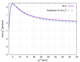
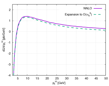
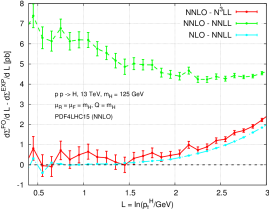
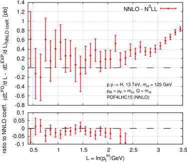
Figure 1: Comparison between the fixed-order transverse momentum distribution for Higgs boson production at $\sqrt{s}=13~{}\mathrm{TeV}$ at NLO (left) and NNLO (right) and the expansion of the N³LL resummation formula given in Eq. (3) to the corresponding order, i.e. ${\cal O}(\alpha_{\mathrm{s}}^{4})$ and ${\cal O}(\alpha_{\mathrm{s}}^{5})$ (namely ${\cal O}(\alpha_{\mathrm{s}}^{2})$ and ${\cal O}(\alpha_{\mathrm{s}}^{3})$ relative to Born), respectively.

Figure 2: Left: difference between the full NLO and NNLO $p_{t}^{\rm H}$ distribution and the expansion of the NNLL and N³LL resummation formulae (3) to the respective perturbative order. Right: difference between the fixed-order NNLO coefficient, i.e. the $\mathcal{O}\left(\alpha_{\mathrm{s}}^{5}\right)$ term alone, and the corresponding coefficient obtained from the expansion of the N³LL resummation.

To perform the matching to fixed order, the resummation formula (3) is expanded up to the third order in the strong coupling. To obtain the expanded results, one can directly set the resolution scale $\delta$ to zero, since the cancellation of IRC divergences is manifest. In Figure 2 we show the comparison between the expansion of the N³LL resummed cross section and the fixed order for the differential distribution of $p_{t}^{\rm H}$ both at NLO (left plot) and at NNLO (right plot). We remind the reader that at the level of the differential distribution NNLO denotes the derivative of the N³LO cumulant, and similarly for lower orders.

In Figure 2 we see that below $p_{t}^{\rm H}\sim 10~{}\mathrm{GeV}$ the fixed-order and the expansion of the resummation are in excellent agreement, and that the size of non-logarithmic terms in the perturbative series remains moderate up to $p_{t}^{\rm H}\sim 50~{}\mathrm{GeV}$.

It is instructive to further investigate the difference between the fixed order and the expansion of the resummation formula in the region of very small $p_{t}^{\rm H}$. In particular, we consider the differential distribution

$$\frac{\mathrm{d}\Sigma(p_{t}^{\rm H})}{\mathrm{d}\ln(p_{t}^{\rm H}/\mathrm{GeV})}\,,$$ (27)

in order to highlight potential logarithmic differences in the $p_{t}^{\rm H}\to 0$ region. A similar validation of the NNLO $p_{t}^{\rm H}$ distribution has been performed in Ref. Chen:2018pzu . The result of our comparison is displayed in the left panel of Figure 2. The dashed green line shows the difference between the NNLO distribution and the ${\cal O}(\alpha_{\mathrm{s}}^{3})$ expansion of the NNLL resummation. As one expects, at small $p_{t}^{\rm H}$ the two predictions for the cumulative distribution differ by a double-logarithmic term (due to the absence of the NNLO coefficient functions and of the two-loop virtual corrections in the NNLL result), which induces a linear slope at the level of the differential distribution (27). When we include the N³LL corrections (solid red line), the difference between the two curves tends to zero, hence proving the consistency between the two predictions. For comparison, the difference between the NLO and NNLL (cyan dot-dashed line) is also reported. The right panel of Figure 2 shows the difference between the NNLO coefficient and the corresponding expansion of the N³LL resummation at the same order. The lower inset of the same figure shows the ratio of the above difference to the NNLO coefficient, which helps quantify the relative difference.

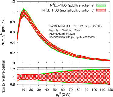
Figure 3: Comparison between additive and multiplicative matching schemes at N³LL+NLO for the transverse momentum distribution for Higgs boson production at $\sqrt{s}=13~{}\mathrm{TeV}$. The lower panel shows the relative uncertainty bands obtained within the two schemes.

As a check on the theoretical setup that will be used in the next sections, it is interesting to compare the predictions for the $p_{t}^{\rm H}$ spectrum obtained with the two matching schemes defined in Eqs. (20) and (25). In order to compare the multiplicative and additive schemes on an equal footing, hence including the same ingredients for both schemes, in this section we consider a matching to NNLO at the level of the cumulative cross section that will allow us to estimate the systematic uncertainty associated with the choice of the matching scheme. In this case the resummed cross section is defined as in Eqs. (20) and (25) with the obvious replacement of ${\rm N^{3}LO}$ by ${\rm NNLO}$. The result of the comparison is reported in Figure 3. We observe a very good agreement between the two matching schemes, which is a sign of robustness of the predictions shown below. The lower panel of Figure 3 shows the relative uncertainty bands obtained within the two schemes, where each prediction is divided by its own central value. The theory uncertainties have a very similar pattern. Given that the difference between the two schemes is always quite moderate with respect to the scale uncertainty, in the following we decide to proceed with the multiplicative prescription (25) as our default. We find analogous conclusions for DY production, and therefore we choose not to report this further comparison here.

4.2 Validation of the expansion for Drell-Yan pair production

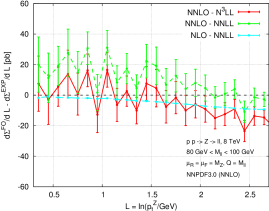
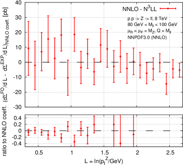
Figure 4: Left: difference between the full NLO and NNLO $p_{t}^{\rm Z}$ distribution and the expansion of the NNLL and N³LL resummation formulae (3) to the respective perturbative order. Right: difference between the fixed-order NNLO coefficient, i.e. the $\mathcal{O}\left(\alpha_{\mathrm{s}}^{3}\right)$ term alone, and the corresponding coefficient obtained from the expansion of the N³LL resummation.

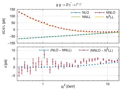
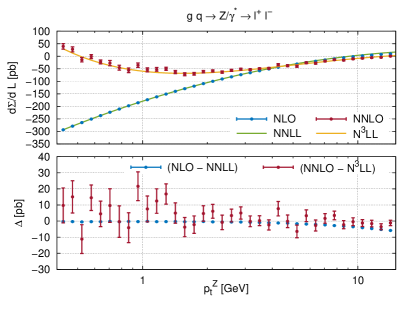
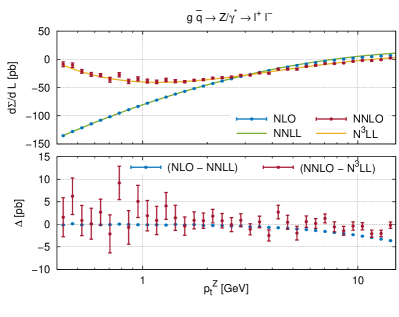
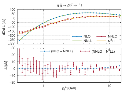
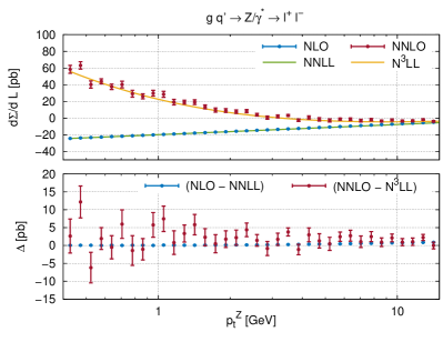
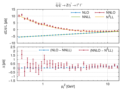
Figure 5: Validation between the fixed-oder coefficients (at NLO and NNLO) and the corresponding expansion of the resummed prediction (at NNLL and N³LL) for the individual partonic channels, with $L=\ln(p_{t}^{\rm Z}/{\rm GeV})$. Note that in contrast to Fig. 4, the curves labelled as “NNLL” only comprises term of $\mathcal{O}\left(\alpha_{\mathrm{s}}^{2}\right)$ and does not include higher-order $\mathcal{O}\left(\alpha_{\mathrm{s}}^{3}\right)$ terms.

Similarly to the validation performed for inclusive Higgs production, in this section we consider the difference between the NNLO differential distribution and the corresponding expansion of the N³LL resummed calculation. In particular, we focus on the differential distribution

$$\frac{\mathrm{d}\Sigma(p_{t}^{\rm Z})}{\mathrm{d}\ln(p_{t}^{\rm Z}/\mathrm{GeV})}\,,$$ (28)

in order to highlight potential logarithmic differences in the $p_{t}^{\rm Z}\to 0$ region.

To perform the validation we consider $8~{}\mathrm{TeV}$ $pp$ collisions with NNPDF3.0 parton densities Ball:2014uwa , and we work within an inclusive setup requiring

$$80~{}\mathrm{GeV} <M_{\ell\ell}<100~{}\mathrm{GeV},$$ (29)

and setting the scales to $\mu_{R}=\mu_{F}=M_{\mathrm{Z}}$ with $x_{Q}=Q/M_{\ell\ell}=1$. This inclusive setup is chosen as to avoid any potential complications due to the use of fiducial cuts, as well as dynamical scales, that act differently on the fixed-order and resummed calculations. Indeed, at variance with the case of the fixed-order calculation, in the resummation both fiducial cuts and dynamical scales are always defined at level of the Born (i.e. $\mathrm{Z}+0$ jet) phase space, which differs from the definition used in the fixed-order calculation unless the extra QCD radiation is extremely soft or collinear to the beam. As a consequence, employing fiducial cuts and/or dynamical scales may necessitate going to smaller values of $p_{t}^{\rm Z}$ in order to see a convergence of the fixed-order to the expansion of the resummation.

The results of the comparison are shown in Figure 4. The left panel displays the difference between the NLO distribution and the expansion of the NNLL resummation to second order (cyan dot-dashed line), and between the NNLO distribution and the expansion of the N³LL resummation to third order (solid red line). In both cases one expects the differences to approach zero at small $p_{t}^{\rm Z}$, which is well confirmed by the plot. In addition, we report on the difference between the NNLO distribution and the expansion of the NNLL resummation to third order given by the dashed green line. Due to missing double-logarithmic terms in the NNLL expansion, a non-vanishing slope is expected in the low-$p_{t}^{\rm Z}$ region, which is suggested by the green curve within statical uncertainties. In order to single out the contribution of the NNLO correction, in the right panel of Figure 4 we show the difference between the NNLO coefficient alone, and the corresponding coefficient in the expansion of the N³LL resummation. As expected, such a difference asymptotically tends to zero for small $p_{t}^{\rm Z}$ values.

In addition to the validation of the full $p_{t}^{\rm Z}$ spectrum shown in Fig. 4, we have further performed the analogous checks for the individual partonic channels which are summarised in Fig. 5. To this end, we have computed the fixed-order NNLO contribution to the $p_{t}^{\rm Z}$ distribution down to $p_{t}^{\rm Z}\sim 0.5~{}\mathrm{GeV}$ with uncertainties at the $10\%$ level. We can clearly observe that the fixed-order prediction is in excellent agreement with the prediction from the resummed calculation for all partonic configurations. The respective bottom panels in each figure show the difference between the two predictions, which for all channels approach zero in the limit $p_{t}^{\rm Z}\to 0$. This is an excellent cross-check of the two calculations, which proves the good numerical stability of the NNLO distributions down to the deep infrared regime.

5 Results for Higgs production in HEFT

In this section we present our predictions for the $p_{t}^{\rm H}$ spectrum both in inclusive $pp\to H$ production, and in the $pp\to H\to\gamma\gamma$ channel with fiducial cuts. The computational setup is the same for both analyses, and all results presented below are obtained in the heavy-top-quark limit. We consider collisions at $13~{}\mathrm{TeV}$, and use parton densities from the PDF4LHC15_nnlo_mc set Butterworth:2015oua ; Dulat:2015mca ; Ball:2014uwa ; Harland-Lang:2014zoa ; Carrazza:2015hva ; Watt:2012tq . The value of the parameter $p$ appearing in the definition of the modified logarithms $\tilde{L}$ is chosen considering the scaling of the spectrum in the hard region, so as to make the matching to the fixed order smooth there. We set $p=4$ as our reference value, but nevertheless have checked that a variation of $p$ by one unit does not induce any significant differences.

We set the central renormalisation and factorisation scales as $\mu_{R}=\mu_{F}=m_{H}/2$, with $m_{H}=125~{}\mathrm{GeV}$, while the resummation scale is chosen to be $x_{Q}=Q/m_{H}=1/2$. We estimate the perturbative uncertainty by performing a seven-scale variation of $\mu_{R}$, $\mu_{F}$ by a factor of two in either direction, while keeping $1/2<\mu_{R}/\mu_{F}<2$ and $x_{Q}=1/2$; Moreover, for central $\mu_{R}$ and $\mu_{F}$ scales, $x_{Q}$ is varied around its central value by a factor of two. The quoted theoretical error is defined as the envelope of all the above variations. We discuss the results for inclusive production in Section 5.1, and then present the predictions for the fiducial distributions in Section 5.2.

5.1 Matched predictions for inclusive Higgs

We start by quantifying the size of the N³LL effects compared to NNLL resummation. In the left plot of Figure 6 we compare the differential distributions at N³LL+NLO and NNLL+NLO in the small-$p_{t}^{\rm H}$ region. The lower panel of the plot shows the ratio of both predictions to the central line of the N³LL+NLO band, which corresponds to central scales in our setup. We observe that N³LL corrections are very moderate in size, with effects of order $2\%$ on the central prediction in most of the displayed range, growing up to at most $5\%$ only in the region of extremely low $p_{t}^{\rm H}$. The central N³LL+NLO result is entirely contained in the NNLL+NLO uncertainty band. On the other hand, the inclusion of the N³LL corrections reduces the perturbative uncertainty for $p_{t}^{\rm H}\lesssim 5~{}\mathrm{GeV}$.

The right plot of Figure 6 shows the same comparison for the matching to NNLO. The effect of the N³LL corrections is consistent with the previous order, with a percent-level correction in most of the range, growing up to $5\%$ at very small $p_{t}^{\rm H}$. Similarly, the perturbative uncertainty is significantly reduced below $10~{}\mathrm{GeV}$ with respect to the NNLL+NNLO case. It is important to stress that in the NNLL+NNLO matching the fixed order and the expansion of the resummation differ by a divergent term $\sim 1/p_{t}^{\rm H}$ at small $p_{t}^{\rm H}$. The fact that the divergence is not visible in the distribution reported in the upper panel of Figure 6 is entirely due to the nature of the multiplicative scheme, which ensures that the distribution follows the resummation scaling at small $p_{t}^{\rm H}$, therefore damping the divergence. A multiplicative matching of N³LL resummation to NNLO was already shown in Ref. Bizon:2017rah , where however no significant reduction in the uncertainty band at small $p_{t}^{\rm H}$ was observed in that case. This feature was due to the limited statistics of the fixed-order distributions used in that analysis at small $p_{t}^{\rm H}$, whose fluctuations dominated the uncertainty band at very small transverse momentum. An additive matching of N³LL to NNLO was recently performed in Ref. Chen:2018pzu .

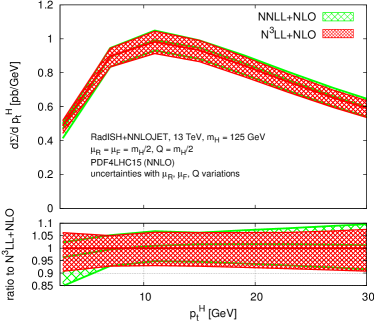
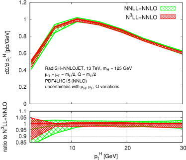
Figure 6: Comparison between different combinations of fixed-order (NLO and NNLO) and resummation (NNLL and N³LL) for the transverse momentum distribution for Higgs boson production at $\sqrt{s}=13~{}\mathrm{TeV}$. Left: NLO and Right: NNLO. The lower panel shows the ratio of predictions to that obtained with N³LL resummation.

Next, we consider the comparison between the matched prediction and the fixed-order one. Figure 7 shows this comparison for two different central scales. The left plot is obtained with central $\mu_{F}=\mu_{R}=m_{H}/2$, while the right plot is obtained with $\mu_{F}=\mu_{R}=m_{H}$. The rest of the setup is kept as described above. We observe that at $\mu_{F}=\mu_{R}=m_{H}/2$ the uncertainty band is affected by cancellations in the scale variation, which accidentally lead to a small perturbative uncertainty. Choosing $m_{H}$ as a central scale (right plot of Figure 7) leads to a broader uncertainty band resulting in a more robust estimate of the perturbative error. This is particularly the case for predictions above $50~{}\mathrm{GeV}$, where resummation effects are progressively less important. We notice indeed that in both cases the effect of resummation starts to be increasingly relevant for $p_{t}^{\rm H}\lesssim 40~{}\mathrm{GeV}$.

In the following we choose $m_{H}/2$ as a central scale. Nevertheless, we stress that a comparison to data (not performed here for Higgs boson production) will require a study of different central-scale choices.

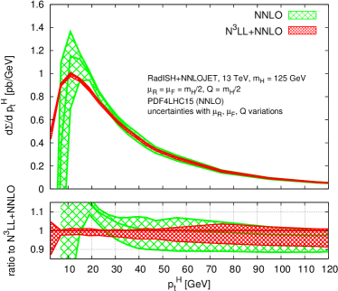
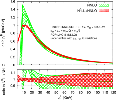
Figure 7: Comparison of the transverse momentum distribution for Higgs boson production at NNLO and N³LL+NNLO for a central scale choice of $\mu_{R}=\mu_{F}=m_{H}/2$ (left) and $\mu_{R}=\mu_{F}=m_{H}$ (right). In both cases, $Q=m_{H}/2$. The lower panel shows the ratio to the N³LL+NNLO prediction.

To conclude, Figure 8 reports the comparison between our best prediction (N³LL+NNLO), the NNLL+NLO, and the NNLO distributions. The plot shows a very good convergence of the predictions at different perturbative orders, with a significant reduction of the scale uncertainty in the whole kinematic range considered here.

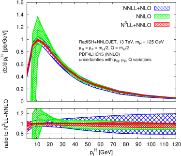
Figure 8: Comparison of the transverse momentum distribution for Higgs boson production between N³LL+NNLO, NNLL+NLO, and NNLO at central scale choice of $\mu_{R}=\mu_{F}=m_{H}/2$. The lower panel shows the ratio to the N³LL+NNLO prediction.

5.2 Matched predictions for fiducial $H\to\gamma\gamma$

Experimental measurements are performed within a fiducial phase-space volume, defined in order to comply with the detector geometry and to enhance signal sensitivity. On the theoretical side it is therefore highly desirable to provide predictions that exactly match the experimental setup. The availability of matched predictions that are fully differential in the Born phase space also allows for a direct comparison to data without relying on Monte Carlo modeling of acceptances. In this section we consider the process $pp\to H\to\gamma\gamma$ and, in particular, we focus on the transverse momentum of the $\gamma\gamma$ system in the presence of fiducial cuts.

The fiducial volume is defined by the set of cuts detailed below Aaboud:2018xdt

$$\min(p_{t}^{\gamma_{1}},p_{t}^{\gamma_{2}})>31.25~{}\mathrm{GeV},\qquad\max(p_{t}^{\gamma_{1}},p_{t}^{\gamma_{2}})>43.75~{}\mathrm{GeV},$$

$$0<|\eta^{\gamma_{1,2}}|<1.37~{}~{}{\rm or}~{}~{}1.52<|\eta^{\gamma_{1,2}}|<2.37,\qquad|Y_{\gamma\gamma}|<2.37\,,$$ (30)

where $p_{t}^{\gamma_{1}}$, $p_{t}^{\gamma_{2}}$ are the transverse momenta of the two photons, $\eta^{\gamma_{i}}$ are their pseudo-rapidities in the hadronic centre-of-mass frame, and $Y_{\gamma\gamma}$ is the photon-pair rapidity. In the definition of the fiducial volume we do not include the photon-isolation requirement, since this would introduce additional logarithmic corrections of non-global nature in the problem, spoiling the formal N³LL+NNLO accuracy of the differential distributions. We consider on-shell Higgs boson production followed by a decay into two photons under the narrow-width approximation with a branching ratio of $2.35\times 10^{-3}$.

In Figure 9 we show the comparison of the matched and the fixed-order predictions for the transverse momentum of the photon pair in the fiducial volume, at different perturbative accuracies: N³LL+NLO vs. NLO in the left panel, and N³LL+NNLO vs. NNLO in the right one.

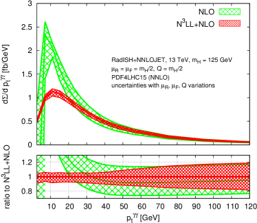
Figure 9: Comparison of the transverse momentum distribution for Higgs boson production at $\sqrt{s}=13~{}\mathrm{TeV}$ in the fiducial volume defined by Eq. (5.2) at N³LL+NLO and NLO (left) and N³LL+NNLO and NNLO (right). The lower panel shows the ratio to the N³LL+NNLO prediction.

By comparing the two panels of Figure 9 we notice a substantial reduction in the theoretical uncertainty in the medium-high-$p_{t}^{\gamma\gamma}$ region, driven by the increase in perturbative accuracy of the fixed-order computation; at very low $p_{t}^{\gamma\gamma}$, the prediction is dominated by resummation, which is common to both panels. The pattern observed in the right panel is very similar to what we obtained in the inclusive case in the left panel of Figure 7. We stress again that the particularly small uncertainty of the matched prediction is to a certain extent due to the choice of central scales we adopt, namely $\mu_{R}=\mu_{F}=m_{H}/2$, which suffers from large accidental cancellations.

6 Results for Drell-Yan production

We now turn to the study of Drell-Yan pair production at the LHC. In this section we present the results for the differential distributions of the transverse momentum of the DY pair, as well as for the angular observable $\phi^{*}_{\eta}$.

We consider $8~{}\mathrm{TeV}$ proton-proton collisions, and compare the resulting calculation for the differential spectra with ATLAS data from Ref. Aad:2015auj . The fiducial phase-space volume is defined as follows:

$$p_{t}^{\ell^{\pm}} >20~{}\mathrm{GeV}, |\eta^{\ell^{\pm}}| <2.4, |Y_{\ell\ell}| <2.4, 46~{}\mathrm{GeV} <M_{\ell\ell}<150~{}\mathrm{GeV},$$ (31)

where $p_{t}^{\ell^{\pm}}$ are the transverse momenta of the two leptons, $\eta^{\ell^{\pm}}$ are their pseudo-rapidities, while $Y_{\ell\ell}$ and $M_{\ell\ell}$ are the rapidity and invariant mass of the di-lepton system, respectively. All rapidities and pseudo-rapidities are evaluated in the hadronic centre-of-mass frame.

For our results, we use parton densities as obtained from the NNPDF3.0 set. The reference value we set for the parameter $p$ appearing in the modified logarithms is $p=4$, but we have checked that a variation of $p$ by one unit does not induce any significant differences.

We set the central scales as $\mu_{R}=\mu_{F}=M_{T}=\sqrt{M_{\ell\ell}^{2}+(p_{t}^{\rm Z})^{2}}$, while the central resummation scale is chosen to be $x_{Q}=Q/M_{\ell\ell}=1/2$. The theoretical uncertainty is estimated through the same set of variations as for Higgs boson production.

The results for $p_{t}^{\rm Z}$ and $\phi^{*}_{\eta}$ are shown in the following two subsections. All plots have the same pattern: the main panels display the comparison of normalised differential distributions at NNLO (green), NNLL+NLO (blue), and N³LL+NNLO (red), respectively, overlaid on ATLAS data points (black). Correspondingly, the lower insets of each panel show the ratio of the theoretical curves to data, with the same colour code as in the main panels.

6.1 Matched predictions for fiducial $p_{t}^{\rm Z}$ distributions

In Figure 10 we display the normalised $p_{t}^{\rm Z}$ distributions in which, in addition to the fiducial cuts reported above, we consider three different lepton-pair invariant-mass windows:

$${\rm low~{}invariant~{}mass:} ~{}46~{}\mathrm{GeV}<M_{\ell\ell}<~{}66~{}\mathrm{GeV},$$

$${\rm medium~{}invariant~{}mass:} ~{}66~{}\mathrm{GeV}<M_{\ell\ell}<116~{}\mathrm{GeV},$$

$${\rm high~{}invariant~{}mass:} 116~{}\mathrm{GeV}<M_{\ell\ell}<150~{}\mathrm{GeV}.$$ (32)

A comparison of the most accurate matched prediction with the fixed-order one shows that the N³LL+NNLO prediction starts differing significantly from the NNLO for $p_{t}^{\rm Z}\lesssim 15~{}\mathrm{GeV}$, while for $p_{t}^{\rm Z}>20~{}\mathrm{GeV}$ the NNLO is sufficient to provide a reliable description. Comparing matched predictions with different formal accuracy, we note that the N³LL+NNLO curve has a significantly reduced theoretical systematics with respect to that for NNLL+NLO, in the whole $p_{t}^{\rm Z}$ range and for all considered invariant-mass windows. The perturbative error is reduced by more than a factor of two at very low $p_{t}^{\rm Z}$, where the prediction is dominated by resummation, and the leftover uncertainty in that region is as small as $3$–$5\%$, and almost comparable with the excellent experimental precision. The shape of the $p_{t}^{\rm Z}$ distributions is also significantly distorted by the inclusion of higher orders: the spectrum is harder than the NNLL+NLO result for $p_{t}^{\rm Z}\gtrsim 10~{}\mathrm{GeV}$, and the peak is lower, with the N³LL+NNLO curves in much better agreement with data with respect to NNLL+NLO in the whole kinematic range. Among the three considered windows, the most accurately described at N³LL+NNLO are the ones at intermediate and high invariant mass; the accuracy very slightly degrades for smaller invariant masses, however the theory uncertainty never gets larger than $5$–$7\%$ over the whole displayed $p_{t}^{\rm Z}$ range.

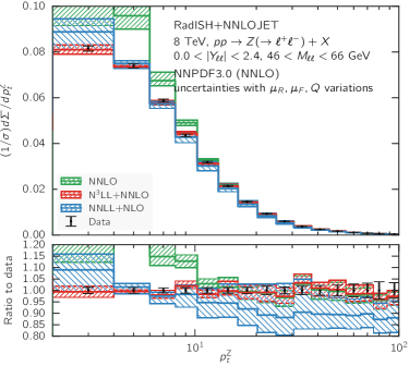
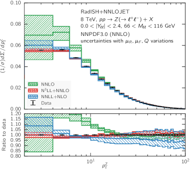
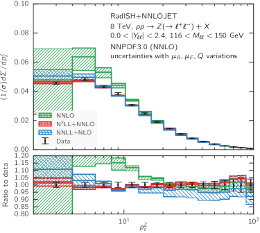
Figure 10: Comparison of the normalised transverse momentum distribution for Drell-Yan pair production at NNLO (green), NNLL+NLO (blue) and N³LL+NNLO (red) at $\sqrt{s}=8~{}\mathrm{TeV}$ integrated over the full lepton-pair rapidity range ($0<|Y_{\ell\ell}|<2.4$), in three different lepton-pair invariant-mass windows. For reference, the ATLAS data is also shown, and the lower panel shows the ratio of each prediction to data.

In Figure 11 we focus our analysis on the central lepton-pair invariant-mass window defined in Eq. (6.1) and show predictions for the normalised $p_{t}^{\rm Z}$ distribution in six different lepton-pair rapidity slices:

(a) $$0.0<\lvert Y_{\ell\ell}\rvert<0.4, 0.4<\lvert Y_{\ell\ell}\rvert<0.8, 0.8<\lvert Y_{\ell\ell}\rvert<1.2,$$ (b) (c)

(d) $$1.2<\lvert Y_{\ell\ell}\rvert<1.6, 1.6<\lvert Y_{\ell\ell}\rvert<2.0, 2.0<\lvert Y_{\ell\ell}\rvert<2.4.$$ (e) (f) (33)

The comments relevant to Figure 10 by far and large apply in this case as well, with our best prediction at N³LL+NNLO affected by an uncertainty that is of order $3$–$5\%$ in the whole $p_{t}^{\rm Z}$ range, regardless of the considered rapidity slice. It is moreover in very good agreement with the experimental data, hence significantly improving on both the NNLL+NLO, in the whole $p_{t}^{\rm Z}$ range, and the pure NNLO, in the $p_{t}^{\rm Z}\lesssim 20~{}\mathrm{GeV}$ region.

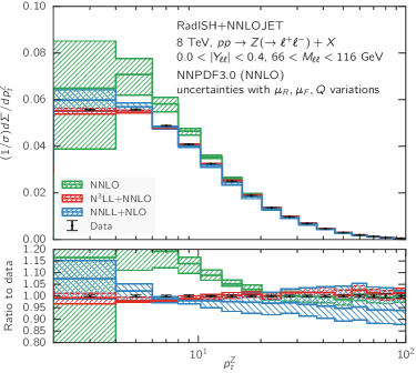
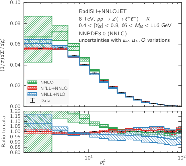
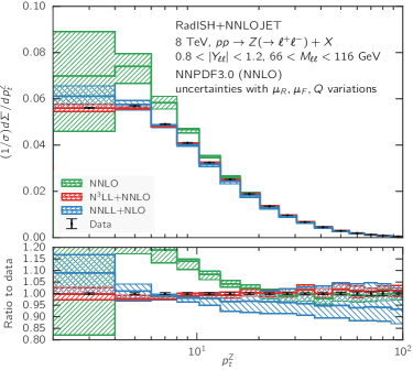
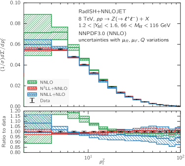
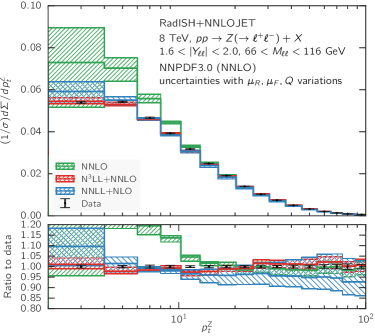
Figure 11: Comparison of the normalised transverse momentum distribution for Drell-Yan pair production at NNLO (green), NNLL+NLO (blue) and N³LL+NNLO (red) at $\sqrt{s}=8~{}\mathrm{TeV}$ in the central lepton-pair invariant-mass window ($66~{}\mathrm{GeV}<M_{\ell\ell}<116~{}\mathrm{GeV}$) for six different lepton-pair rapidity slices. For reference, the ATLAS data is also shown, and the lower panel shows the ratio of each prediction to data.

6.2 Matched predictions for fiducial $\phi^{*}_{\eta}$ distributions

Figure 12 shows the $\phi^{*}_{\eta}$ distribution for three different lepton-pair invariant-mass windows as defined in Eq. (6.1).

The pattern of comparisons among theoretical predictions is qualitatively similar to what discussed for the $p_{t}^{\rm Z}$ distribution. Resummation effects at N³LL+NNLO start being important with respect to the pure NNLO in the region $\phi^{*}_{\eta}\lesssim 0.2$; the shape of the N³LL+NNLO distribution is significantly distorted with respect to the NNLL+NLO one in a similar fashion as for the $p_{t}^{\rm Z}$ case, and the uncertainty band is reduced by a factor of two or more over the whole range and for all invariant-mass windows, down to the level of $3$–$5\%$ (except at low invariant mass, where the uncertainty is $5$–$7\%$).

At variance with the $p_{t}^{\rm Z}$ case, however, for $\phi^{*}_{\eta}$ we note that the N³LL+NNLO prediction describes data appropriately only in the central- and high- invariant-mass windows. In the low-invariant-mass one, the prediction undershoots data in the medium-hard region, by up to $5$–$7\%$. This tension was already observed in the fixed-order NNLO comparison Gehrmann-DeRidder:2016jns . However, given the large statistical uncertainty of the data in this invariant-mass range, the theory still provides a reasonable description of the measurement, and the N³LL+NNLO prediction is in much better agreement with data than the NNLL+NLO in the whole range of $\phi^{*}_{\eta}$, especially at low $\phi^{*}_{\eta}$.

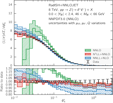
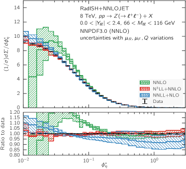
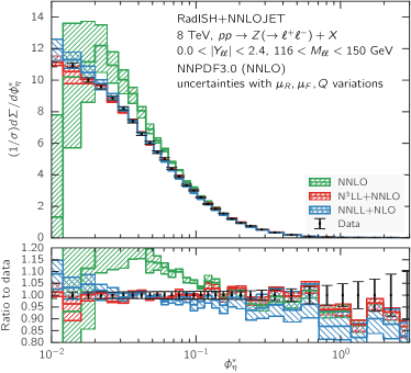
Figure 12: Comparison of the normalised $\phi^{*}_{\eta}$ distribution for Drell-Yan pair production at NNLO (green), NNLL+NLO (blue) and N³LL+NNLO (red) at $\sqrt{s}=8~{}\mathrm{TeV}$ integrated over the full lepton-pair rapidity range ($0<|Y_{\ell\ell}|<2.4$), in three different lepton-pair invariant-mass windows. For reference, the ATLAS data is also shown, and the lower panel shows the ratio of each prediction to data.

In Figure 13 we show the results for the $\phi^{*}_{\eta}$ distributions in the central invariant-mass window, see Eq. (6.1), split into the six lepton-pair rapidity slices described in Eq. (6.1). Moreover, given the availability of experimental measurements, in Figures 14 and 15 we also provide predictions sliced in $Y_{\ell\ell}$ for the low- and high- di-lepton invariant-mass windows, respectively. The three rapidity slices we focus on correspond to regions (a+b), (c+d), and (e+f) of Eq. (6.1).

The prediction subdivided in rapidity slices largely shares the same features as that integrated over rapidity, which has been detailed in Figure 12. In the central invariant-mass window, data is accurately reproduced by the N³LL+NNLO prediction, regardless of the considered rapidity slice, with a theoretical systematics in the $5\%$ range or smaller. The quality of the description slightly degrades at low invariant mass, and to a lesser extent also at high invariant mass, mainly in the hard region, with a pattern similar to that displayed by the rapidity-integrated spectrum. Overall, the uncertainty associated with the N³LL+NNLO is of order of $5\%$ or better, with a significant improvement both in the shape and in the systematics with respect to NNLL+NLO.

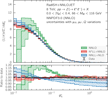
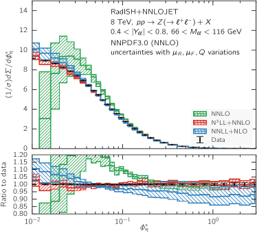
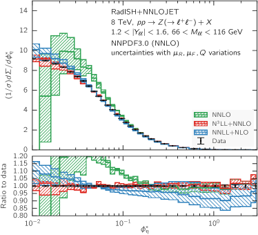
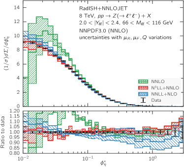
Figure 13: Comparison of the normalised $\phi^{*}_{\eta}$ distribution for Drell-Yan pair production at NNLO (green), NNLL+NLO (blue) and N³LL+NNLO (red) at $\sqrt{s}=8~{}\mathrm{TeV}$ in the central lepton-pair invariant-mass window ($66~{}\mathrm{GeV}<M_{\ell\ell}<116~{}\mathrm{GeV}$) for three different lepton-pair rapidity slices. For reference, the ATLAS data is also shown, and the lower panel shows the ratio of each prediction to data.

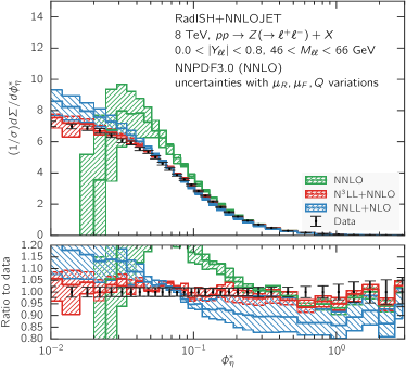
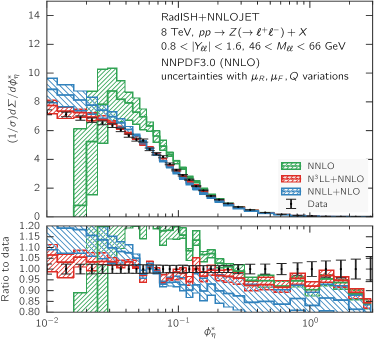
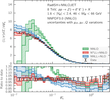
Figure 14: Comparison of the normalised $\phi^{*}_{\eta}$ distribution for Drell-Yan pair production at NNLO (green), NNLL+NLO (blue) and N³LL+NNLO (red) at $\sqrt{s}=8~{}\mathrm{TeV}$ in the low lepton-pair invariant-mass window ($46~{}\mathrm{GeV}<M_{\ell\ell}<66~{}\mathrm{GeV}$) for three different lepton-pair rapidity slices. For reference, the ATLAS data is also shown, and the lower panel shows the ratio of each prediction to data.

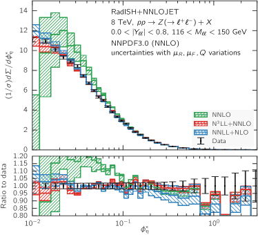
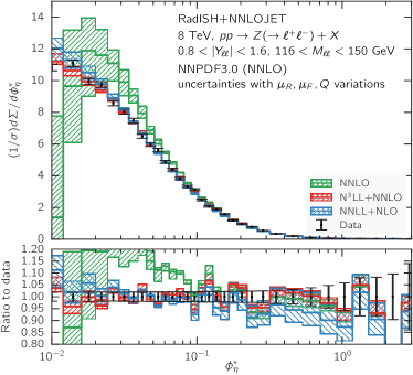
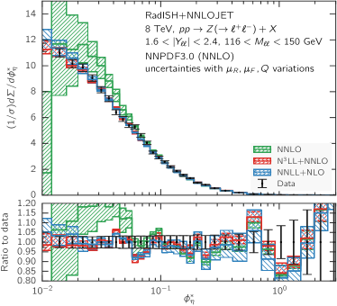
Figure 15: Comparison of the normalised $\phi^{*}_{\eta}$ distribution for Drell-Yan pair production at NNLO (green), NNLL+NLO (blue) and N³LL+NNLO (red) at $\sqrt{s}=8~{}\mathrm{TeV}$ in the high lepton-pair invariant-mass window ($116~{}\mathrm{GeV}<M_{\ell\ell}<150~{}\mathrm{GeV}$) for three different lepton-pair rapidity slices. For reference, the ATLAS data is also shown, and the lower panel shows the ratio of each prediction to data.

7 Conclusions

In this work we have presented precise predictions for differential distributions in Higgs boson and Drell-Yan pair production at the LHC at N³LL+NNLO.

The resummation is performed in momentum space and is fully exclusive in the Born phase space. For the matching to NNLO we adopted a multiplicative scheme, which allows for the inclusion of the N³LO constant terms to the cumulative cross section. These are currently unknown analytically, but can be included numerically once the total N³LO cross section has been obtained. The uncertainty associated with the choice of the matching scheme was estimated at NLO accuracy, for which an additive matching with the same ingredients can be also performed. At this order the predictions obtained with the two prescriptions are in very good agreement with each other, and the matching-scheme uncertainty is under control within the perturbative error.

For Higgs boson production in gluon fusion, we have considered the transverse-momentum spectrum both at the inclusive level and in the $H\rightarrow\gamma\gamma$ channel within ATLAS fiducial cuts. In both cases, we observe that the resummation reduces the theoretical uncertainties and stabilises the fixed-order result below $p_{t}^{\rm H}\sim 40~{}\mathrm{GeV}$. The effects of the N³LL corrections with respect to NNLL+NNLO distributions are moderate in size, with a percent-level correction in most of the range, growing up to $5\%$ at very small $p_{t}^{\rm H}$. However, the perturbative uncertainty is reduced significantly below $10~{}\mathrm{GeV}$ with respect to the NNLL+NNLO case.

For Drell-Yan pair production, we have presented resummed predictions within ATLAS fiducial cuts Aad:2015auj both for the normalised $p_{t}^{\rm Z}$ distributions and for the normalised $\phi^{*}_{\eta}$ distributions, and we have compared them to experimental data. In the case of transverse-momentum distributions, the difference between the fixed-order and the N³LL+NNLO result becomes significant for $p_{t}^{\rm Z}<10$–$15~{}\mathrm{GeV}$, while for $p_{t}^{\rm Z}>20~{}\mathrm{GeV}$ the NNLO prediction is sufficient to provide a reliable description of the experimental data. Comparing matched results with different formal accuracy, we note that the N³LL+NNLO prediction has a significantly reduced theoretical uncertainty with respect to that for NNLL+NLO, in the whole $p_{t}^{\rm Z}$ range and for all invariant-mass windows considered in our study.

For the $\phi^{*}_{\eta}$ distribution, resummation effects start being important with respect to pure NNLO in the region $\phi^{*}_{\eta}\lesssim 0.2$. At N³LL+NNLO the shape of the distribution is significantly distorted with respect to that for NNLL+NLO (the spectrum is hardened in the tail, and the height of the peak is lowered), and the uncertainty band is reduced by a factor of two or more over the whole range of $\phi^{*}_{\eta}$ and for most invariant-mass windows, down to the level of $3$–$5\%$. An exception is at low invariant mass, where the uncertainty remains in the $5$–$7\%$ range. Unlike the $p_{t}^{\rm Z}$ case, for $\phi^{*}_{\eta}$ we note that the N³LL+NNLO prediction describes data appropriately only in the central- and high-invariant-mass windows, while at low invariant mass the prediction undershoots the data in the medium-hard region. The difference between the central values of the data and theory here can be of the order of $10\%$, however no significant tension with the data is observed, due to the sizeable statistical uncertainty in the measurement. The agreement in these invariant-mass bins is much improved by the inclusion of the N³LL+NNLO corrections with respect to the NNLL+NLO distribution.

Our results are an important step in the LHC precision programme, where accurate predictions have become necessary for an appropriate interpretation and exploitation of data. In order to improve on the predictions presented here, several effects must be considered.

For Higgs boson production via gluon fusion, the impact of other heavy quarks, notably the bottom quark, becomes relevant at this level of accuracy and therefore must be taken into account. Recent studies show that the effect of the top-bottom interference at NNLL+NLO Lindert:2017pky ; Caola:2018zye could lead to distortions of the transverse-momentum spectrum that are as large as $\sim 5\%$ with respect to the HEFT approximation, and the theory uncertainties associated with this contribution are of ${\cal O}(20\%)$. These effects are therefore of the same order as the perturbative uncertainties presented here, and must be included for a consistent prediction of the spectrum with $5$–$10\%$ perturbative accuracy in the region $p_{t}^{\rm H}\lesssim m_{H}$.

In the DY case, the situation is more involved given the smaller perturbative uncertainty. At this level of precision, it is necessary to supplement the predictions obtained in this work at small $p_{t}^{\rm Z}$ and $\phi^{*}_{\eta}$ with QED corrections and with an estimate of various sources of non-perturbative effects that could be as large as a few $\%$ in this region. Similarly, the inclusion of quark masses may have a few-percent effect on the spectrum Pietrulewicz:2017gxc ; Bagnaschi:2018dnh , and more precise studies are necessary in order to assess their impact precisely. Recent analyses Bagnaschi:2018dnh suggest that the inclusion of these effects may have a non-negligible impact on observables of current phenomenological interest, such as the determination of the $W$-boson mass Aaboud:2017svj . Given that the size of these effects is of the order of the perturbative uncertainty of the N³LL+NNLO prediction, a careful assessment will be necessary to improve further on the results presented in this work.

Appendix A Formulae for the matching schemes

In this appendix we report the necessary formulae to implement the matching schemes defined in Eqs. (20) and (25) and used in our study. We start by introducing a convenient notation for the perturbative expansion of the various ingredients. We define

$$\sigma_{\rm tot}^{\rm N^{3}LO}=\sum_{i=0}^{3}\sigma^{(i)},\qquad\Sigma^{\rm N^{3}LO}(v)=\sigma^{(0)}+\sum_{i=1}^{3}\Sigma^{(i)}(v),$$ (34)

where

$$\Sigma^{(i)}(v)=\sigma^{(i)}+\bar{\Sigma}^{(i)}(v),\qquad\bar{\Sigma}^{(i)}(v)\equiv-\int_{v}^{\infty}\mathrm{d}v^{\prime}\;\frac{\mathrm{d}\Sigma^{(i)}(v^{\prime})}{\mathrm{d}v^{\prime}}.$$ (35)

Moreover, we denote the perturbative expansion of the resummed cross section $\Sigma^{\rm N^{k}LL}$ as

$$\Sigma^{\rm EXP}(v)=\sigma^{(0)}+\sum_{i=1}^{3}\Sigma_{\rm N^{k}LL}^{(i)}(v).$$ (36)

With this notation, the additive scheme of Eq. (20) becomes (for simplicity we drop the explicit dependence on $v$ in the following)

$$\Sigma_{\rm add}^{\rm MAT}= \Sigma^{\rm N^{k}LL}+\left\{\sigma^{(1)}+\bar{\Sigma}^{(1)}-\Sigma_{\rm N^{k}LL}^{(1)}\right\}+\left\{\sigma^{(2)}+\bar{\Sigma}^{(2)}-\Sigma_{\rm N^{k}LL}^{(2)}\right\}+\left\{\sigma^{(3)}+\bar{\Sigma}^{(3)}-\Sigma_{\rm N^{k}LL}^{(3)}\right\},$$ (37)

where the three terms in curly brackets denote the NLO, NNLO and N³LO contributions to the matching, respectively.

For the multiplicative scheme we need to introduce the asymptotic expansion $\Sigma^{\rm N^{k}LL}_{\rm asym.}$, defined in Eq. (24) (the definition for $k\neq 3$ is analogous with obvious replacements) in terms of the $\tilde{L}\to 0$ limit of the coefficients $\tilde{\cal L}_{\rm N^{k}LL}$ of Eqs. (12), (3), (3), which read

$$\tilde{\cal L}_{\rm NLL}^{\tilde{L}\to 0} =\sum_{c,c^{\prime}}\frac{\mathrm{d}|\mathcal{M}_{B}|_{cc^{\prime}}^{2}}{\mathrm{d}\Phi_{B}}f_{c}\!\left(\mu_{F},x_{1}\right)f_{c^{\prime}}\!\left(\mu_{F},x_{2}\right),$$

$$\tilde{\cal L}_{\rm NNLL}^{\tilde{L}\to 0} =\sum_{c,c^{\prime}}\frac{\mathrm{d}|\mathcal{M}_{B}|_{cc^{\prime}}^{2}}{\mathrm{d}\Phi_{B}}\sum_{i,j}\int_{x_{1}}^{1}\frac{\mathrm{d}z_{1}}{z_{1}}\int_{x_{2}}^{1}\frac{\mathrm{d}z_{2}}{z_{2}}f_{i}\!\left(\mu_{F},\frac{x_{1}}{z_{1}}\right)f_{j}\!\left(\mu_{F},\frac{x_{2}}{z_{2}}\right)$$

$$\times\Bigg{\{}\delta_{ci}\delta_{c^{\prime}j}\delta(1-z_{1})\delta(1-z_{2})\left(1+\frac{\alpha_{\mathrm{s}}(\mu_{R})}{2\pi}\tilde{H}^{(1)}(\mu_{R},x_{Q})\right)$$

$$+\frac{\alpha_{\mathrm{s}}(\mu_{R})}{2\pi}\left(\tilde{C}_{ci}^{(1)}(z_{1},\mu_{F},x_{Q})\delta(1-z_{2})\delta_{c^{\prime}j}+\{z_{1}\leftrightarrow z_{2};c,i\leftrightarrow c^{\prime}j\}\right)\Bigg{\}},$$

$$\tilde{\cal L}_{\rm N^{3}LL}^{\tilde{L}\to 0} =\sum_{c,c^{\prime}}\frac{\mathrm{d}|\mathcal{M}_{B}|_{cc^{\prime}}^{2}}{\mathrm{d}\Phi_{B}}\sum_{i,j}\int_{x_{1}}^{1}\frac{\mathrm{d}z_{1}}{z_{1}}\int_{x_{2}}^{1}\frac{\mathrm{d}z_{2}}{z_{2}}f_{i}\!\left(\mu_{F},\frac{x_{1}}{z_{1}}\right)f_{j}\!\left(\mu_{F},\frac{x_{2}}{z_{2}}\right)$$

$$\times\Bigg{\{}\delta_{ci}\delta_{c^{\prime}j}\delta(1-z_{1})\delta(1-z_{2})\left(1+\frac{\alpha_{\mathrm{s}}(\mu_{R})}{2\pi}\tilde{H}^{(1)}(\mu_{R},x_{Q})+\frac{\alpha_{\mathrm{s}}^{2}(\mu_{R})}{(2\pi)^{2}}\tilde{H}^{(2)}(\mu_{R},x_{Q})\right)$$

$$+\frac{\alpha_{\mathrm{s}}(\mu_{R})}{2\pi}\left(\tilde{C}_{ci}^{(1)}(z_{1},\mu_{F},x_{Q})\delta(1-z_{2})\delta_{c^{\prime}j}+\{z_{1}\leftrightarrow z_{2};c,i\leftrightarrow c^{\prime},j\}\right)$$

$$+\frac{\alpha_{\mathrm{s}}^{2}(\mu_{R})}{(2\pi)^{2}}\left(\tilde{C}_{ci}^{(2)}(z_{1},\mu_{F},x_{Q})\delta(1-z_{2})\delta_{c^{\prime}j}+\{z_{1}\leftrightarrow z_{2};c,i\leftrightarrow c^{\prime},j\}\right)$$

$$+\frac{\alpha_{\mathrm{s}}^{2}(\mu_{R})}{(2\pi)^{2}}\Big{(}\tilde{C}_{ci}^{(1)}(z_{1},\mu_{F},x_{Q})\tilde{C}_{c^{\prime}j}^{(1)}(z_{2},\mu_{F},x_{Q})+G_{ci}^{(1)}(z_{1})G_{c^{\prime}j}^{(1)}(z_{2})\Big{)}$$

$$+\frac{\alpha_{\mathrm{s}}^{2}(\mu_{R})}{(2\pi)^{2}}\tilde{H}^{(1)}(\mu_{R},x_{Q})\Big{(}\tilde{C}_{ci}^{(1)}(z_{1},\mu_{F},x_{Q})\delta(1-z_{2})\delta_{c^{\prime}j}+\{z_{1}\leftrightarrow z_{2};c,i\leftrightarrow c^{\prime},j\}\Big{)}\Bigg{\}}.$$ (38)

In the following formula the perturbative expansion of $\Sigma^{\rm N^{k}LL}_{\rm asym.}$ is denoted as follows

$$\Sigma^{\rm N^{k}LL}_{\rm asym.}=\sigma^{(0)}+\sum_{i=1}^{k-1}\Sigma_{\rm asym.}^{(i)}.$$ (39)

With this notation the matching formula (25) reads

$$\Sigma_{\rm mult}^{\rm MAT}(v)=\frac{\Sigma^{\rm N^{k}LL}}{\Sigma^{\rm N^{k}LL}_{\rm asym.}}\Bigg{[}\sigma^{(0)}+\left\{\sigma^{(1)}+\bar{\Sigma}^{(1)}+\Sigma_{\rm asym.}^{(1)}-\Sigma_{\rm N^{k}LL}^{(1)}\right\}$$

$$+\left\{\sigma^{(2)}+\bar{\Sigma}^{(2)}+\Sigma_{\rm asym.}^{(2)}-\Sigma_{\rm N^{k}LL}^{(2)}+\frac{\Sigma_{\rm asym.}^{(1)}}{\sigma^{(0)}}\left(\sigma^{(1)}+\bar{\Sigma}^{(1)}\right)+\frac{(\Sigma_{\rm N^{k}LL}^{(1)})^{2}}{\sigma^{(0)}}-\frac{\Sigma_{\rm N^{k}LL}^{(1)}}{\sigma^{(0)}}\left(\sigma^{(1)}+\bar{\Sigma}^{(1)}+\Sigma_{\rm asym.}^{(1)}\right)\right\}$$

$$+\Bigg{\{}\sigma^{(3)}+\bar{\Sigma}^{(3)}-\Sigma_{\rm N^{k}LL}^{(3)}-\frac{(\Sigma_{\rm N^{k}LL}^{(1)})^{3}}{(\sigma^{(0)})^{2}}+\frac{(\Sigma_{\rm N^{k}LL}^{(1)})^{2}}{(\sigma^{(0)})^{2}}\left(\sigma^{(1)}+\bar{\Sigma}^{(1)}+\Sigma_{\rm asym.}^{(1)}\right)$$

$$+\frac{1}{\sigma_{0}}\left((\sigma^{(1)}+\bar{\Sigma}^{(1)})(\Sigma_{\rm asym.}^{(2)}-\Sigma_{\rm N^{k}LL}^{(2)})+\Sigma_{\rm asym.}^{(1)}(\sigma^{(2)}+\bar{\Sigma}^{(2)}-\Sigma_{\rm N^{k}LL}^{(2)})\right)$$

$$-\frac{1}{(\sigma^{(0)})^{2}}\Sigma_{\rm N^{k}LL}^{(1)}\left(\Sigma_{\rm asym.}^{(1)}(\sigma^{(1)}+\bar{\Sigma}^{(1)})+\sigma^{(0)}(\sigma^{(2)}+\bar{\Sigma}^{(2)}+\Sigma_{\rm asym.}^{(2)}-2\Sigma_{\rm N^{k}LL}^{(2)})\right)\Bigg{\}}\Bigg{]},$$ (40)

where, as above, we grouped the terms entering at NLO, NNLO, and N³LO within curly brackets.

Appendix B Formulae for N³LL resummation

In this section we report the expressions for quantities needed for N³LL resummation of transverse observables, that we have used throughout this article.

First of all we report our convention for the RG equation of the strong coupling which reads

$$\frac{\mathrm{d}\alpha_{\mathrm{s}}(\mu)}{\mathrm{d}\ln\mu^{2}}=\beta(\alpha_{\mathrm{s}})\equiv-\alpha_{\mathrm{s}}\left(\beta_{0}\alpha_{\mathrm{s}}+\beta_{1}\alpha_{\mathrm{s}}^{2}+\beta_{2}\alpha_{\mathrm{s}}^{3}+\beta_{3}\alpha_{\mathrm{s}}^{4}+\dots\right),$$ (41)

where the coefficients of the $\beta$-function are

$$\beta_{0} = \frac{11C_{A}-2n_{f}}{12\pi}\,,\qquad\beta_{1}=\frac{17C_{A}^{2}-5C_{A}n_{f}-3C_{F}n_{f}}{24\pi^{2}}\,,$$ (42)

$$\beta_{2} = \frac{2857C_{A}^{3}+(54C_{F}^{2}-615C_{F}C_{A}-1415C_{A}^{2})n_{f}+(66C_{F}+79C_{A})n_{f}^{2}}{3456\pi^{3}}\,,$$ (43)

$$\beta_{3} = \frac{1}{(4\pi)^{4}}\Bigg{\{}C_{A}C_{F}n_{f}^{2}\frac{1}{4}\left(\frac{17152}{243}+\frac{448}{9}\zeta_{3}\right)+C_{A}C_{F}^{2}n_{f}\frac{1}{2}\left(-\frac{4204}{27}+\frac{352}{9}\zeta_{3}\right)$$ (44)

$$\hskip 28.45274pt+\frac{53}{243}C_{A}n_{f}^{3}+C_{A}^{2}C_{F}n_{f}\frac{1}{2}\left(\frac{7073}{243}-\frac{656}{9}\zeta_{3}\right)+C_{A}^{2}n_{f}^{2}\frac{1}{4}\left(\frac{7930}{81}+\frac{224}{9}\zeta_{3}\right)$$

$$\hskip 28.45274pt+\frac{154}{243}C_{F}n_{f}^{3}+C_{A}^{3}n_{f}\frac{1}{2}\left(-\frac{39143}{81}+\frac{136}{3}\zeta_{3}\right)+C_{A}^{4}\left(\frac{150653}{486}-\frac{44}{9}\zeta_{3}\right)$$

$$\hskip 28.45274pt+C_{F}^{2}n_{f}^{2}\frac{1}{4}\left(\frac{1352}{27}-\frac{704}{9}\zeta_{3}\right)+23C_{F}^{3}n_{f}+n_{f}\frac{d_{F}^{abcd}d_{A}^{abcd}}{N_{A}}\left(\frac{512}{9}-\frac{1664}{3}\zeta_{3}\right)$$

$$\hskip 28.45274pt+n_{f}^{2}\frac{d_{F}^{abcd}d_{F}^{abcd}}{N_{A}}\left(-\frac{704}{9}+\frac{512}{3}\zeta_{3}\right)+\frac{d_{A}^{abcd}d_{A}^{abcd}}{N_{A}}\left(-\frac{80}{9}+\frac{704}{3}\zeta_{3}\right)\Bigg{\}}\,,$$

with

$$\frac{d_{F}^{abcd}d_{F}^{abcd}}{N_{A}}=\frac{N_{c}^{4}-6N_{c}^{2}+18}{96N_{c}^{2}},\qquad\frac{d_{F}^{abcd}d_{A}^{abcd}}{N_{A}}=\frac{N_{c}(N_{c}^{2}+6)}{48},\qquad\frac{d_{A}^{abcd}d_{A}^{abcd}}{N_{A}}=\frac{N_{c}^{2}(N_{c}^{2}+36)}{24},$$

and $C_{A}=N_{c}$, $C_{F}=\frac{N_{c}^{2}-1}{2N_{c}}$, and $N_{c}=3$.

We also provide expressions for the functions $g_{i}(\lambda)$ entering in the N³LL Sudakov radiator Eq. (9) and its derivative. We define

$$\lambda=\alpha_{\mathrm{s}}(\mu_{R})\beta_{0}\tilde{L}\,.$$ (45)

We have:

$$g_{1}(\lambda)= \frac{A^{(1)}}{\pi\beta_{0}}\frac{2\lambda+\ln(1-2\lambda)}{2\lambda},$$ (46)

$$g_{2}(\lambda)= \frac{1}{2\pi\beta_{0}}\ln(1-2\lambda)\left(A^{(1)}\ln\frac{1}{x_{Q}^{2}}+B^{(1)}\right)-\frac{A^{(2)}}{4\pi^{2}\beta_{0}^{2}}\frac{2\lambda+(1-2\lambda)\ln(1-2\lambda)}{1-2\lambda}$$

$$+A^{(1)}\bigg{(}-\frac{\beta_{1}}{4\pi\beta_{0}^{3}}\frac{\ln(1-2\lambda)((2\lambda-1)\ln(1-2\lambda)-2)-4\lambda}{1-2\lambda}$$

$$\hskip 28.45274pt-\frac{1}{2\pi\beta_{0}}\frac{(2\lambda(1-\ln(1-2\lambda))+\ln(1-2\lambda))}{1-2\lambda}\ln\frac{\mu_{R}^{2}}{x_{Q}^{2}M^{2}}\bigg{)}\,,$$ (47)

$$g_{3}(\lambda)= \left(A^{(1)}\ln\frac{1}{x_{Q}^{2}}+B^{(1)}\right)\bigg{(}-\frac{\lambda}{1-2\lambda}\ln\frac{\mu_{R}^{2}}{x_{Q}^{2}M^{2}}+\frac{\beta_{1}}{2\beta_{0}^{2}}\frac{2\lambda+\ln(1-2\lambda)}{1-2\lambda}\bigg{)}$$

$$-\frac{1}{2\pi\beta_{0}}\frac{\lambda}{1-2\lambda}\left(A^{(2)}\ln\frac{1}{x_{Q}^{2}}+B^{(2)}\right)-\frac{A^{(3)}}{4\pi^{2}\beta_{0}^{2}}\frac{\lambda^{2}}{(1-2\lambda)^{2}}$$

$$+A^{(2)}\bigg{(}\frac{\beta_{1}}{4\pi\beta_{0}^{3}}\frac{2\lambda(3\lambda-1)+(4\lambda-1)\ln(1-2\lambda)}{(1-2\lambda)^{2}}-\frac{1}{\pi\beta_{0}}\frac{\lambda^{2}}{(1-2\lambda)^{2}}\ln\frac{\mu_{R}^{2}}{x_{Q}^{2}M^{2}}\bigg{)}$$

$$+A^{(1)}\bigg{(}\frac{\lambda\left(\beta_{0}\beta_{2}(1-3\lambda)+\beta_{1}^{2}\lambda\right)}{\beta_{0}^{4}(1-2\lambda)^{2}}+\frac{(1-2\lambda)\ln(1-2\lambda)\left(\beta_{0}\beta_{2}(1-2\lambda)+2\beta_{1}^{2}\lambda\right)}{2\beta_{0}^{4}(1-2\lambda)^{2}}$$

$$\hskip 28.45274pt+\frac{\beta_{1}^{2}}{4\beta_{0}^{4}}\frac{(1-4\lambda)\ln^{2}(1-2\lambda)}{(1-2\lambda)^{2}}-\frac{\lambda^{2}}{(1-2\lambda)^{2}}\ln^{2}\frac{\mu_{R}^{2}}{x_{Q}^{2}M^{2}}$$

$$\hskip 28.45274pt-\frac{\beta_{1}}{2\beta_{0}^{2}}\frac{(2\lambda(1-2\lambda)+(1-4\lambda)\ln(1-2\lambda))}{(1-2\lambda)^{2}}\ln\frac{\mu_{R}^{2}}{x_{Q}^{2}M^{2}}\bigg{)}\,,$$ (48)

$$g_{4}(\lambda)= \frac{A^{(4)}(3-2\lambda)\lambda^{2}}{24\pi^{2}\beta_{0}^{2}(2\lambda-1)^{3}}$$

$$+\frac{A^{(3)}}{48\pi\beta_{0}^{3}(2\lambda-1)^{3}}\Bigg{\{}3\beta_{1}(1-6\lambda)\ln(1-2\lambda)+2\lambda\Bigg{(}\beta_{1}(5\lambda(2\lambda-3)+3)$$

$$\hskip 28.45274pt+6\beta_{0}^{2}(3-2\lambda)\lambda\ln\frac{\mu_{R}^{2}}{x_{Q}^{2}M^{2}}\Bigg{)}+12\beta_{0}^{2}(\lambda-1)\lambda(2\lambda-1)\ln\frac{1}{x_{Q}^{2}}\Bigg{\}}$$

$$+\frac{A^{(2)}}{24\beta_{0}^{4}(2\lambda-1)^{3}}\Bigg{\{}32\beta_{0}\beta_{2}\lambda^{3}-2\beta_{1}^{2}\lambda(\lambda(22\lambda-9)+3)$$

$$\hskip 28.45274pt+12\beta_{0}^{4}(3-2\lambda)\lambda^{2}\ln^{2}\frac{\mu_{R}^{2}}{x_{Q}^{2}M^{2}}+6\beta_{0}^{2}\ln\frac{\mu_{R}^{2}}{x_{Q}^{2}M^{2}}\times$$

$$\hskip 28.45274pt\left(\beta_{1}(1-6\lambda)\ln(1-2\lambda)+2(\lambda-1)\lambda(2\lambda-1)\left(\beta_{1}+2\beta_{0}^{2}\ln\frac{1}{x_{Q}^{2}}\right)\right)$$

$$\hskip 28.45274pt+3\beta_{1}\Bigg{(}\beta_{1}\ln(1-2\lambda)(2\lambda+(6\lambda-1)\ln(1-2\lambda)-1)$$

$$\hskip 28.45274pt-2\beta_{0}^{2}(2\lambda-1)(2(\lambda-1)\lambda-\ln(1-2\lambda))\ln\frac{1}{x_{Q}^{2}}\Bigg{)}\Bigg{\}}$$

$$+\frac{\pi A^{(1)}}{12\beta_{0}^{5}(2\lambda-1)^{3}}\Bigg{\{}\beta_{1}^{3}(1-6\lambda)\ln^{3}(1-2\lambda)+3\ln(1-2\lambda)\Bigg{(}\beta_{0}^{2}\beta_{3}(2\lambda-1)^{3}$$

$$\hskip 28.45274pt+\beta_{0}\beta_{1}\beta_{2}\left(1-2\lambda\left(8\lambda^{2}-4\lambda+3\right)\right)+4\beta_{1}^{3}\lambda^{2}(2\lambda+1)$$

$$\hskip 28.45274pt+\beta_{0}^{2}\beta_{1}\ln\frac{\mu_{R}^{2}}{x_{Q}^{2}M^{2}}\left(\beta_{0}^{2}(1-6\lambda)\ln\frac{\mu_{R}^{2}}{x_{Q}^{2}M^{2}}-4\beta_{1}\lambda\right)\Bigg{)}$$

$$\hskip 28.45274pt+3\beta_{1}^{2}\ln^{2}(1-2\lambda)\left(2\beta_{1}\lambda+\beta_{0}^{2}(6\lambda-1)\ln\frac{\mu_{R}^{2}}{x_{Q}^{2}M^{2}}\right)$$

$$\hskip 28.45274pt+3\beta_{0}^{2}(2\lambda-1)\ln\frac{1}{x_{Q}^{2}}\Bigg{(}-\beta_{1}^{2}\ln^{2}(1-2\lambda)+2\beta_{0}^{2}\beta_{1}\ln(1-2\lambda)\ln\frac{\mu_{R}^{2}}{x_{Q}^{2}M^{2}}$$

$$\hskip 28.45274pt+4\lambda\left(\lambda\left(\beta_{1}^{2}-\beta_{0}\beta_{2}\right)+\beta_{0}^{4}(\lambda-1)\ln^{2}\frac{\mu_{R}^{2}}{x_{Q}^{2}M^{2}}\right)\Bigg{)}$$

$$\hskip 28.45274pt+2\lambda\Bigg{(}\beta_{0}^{2}\beta_{3}((15-14\lambda)\lambda-3)+\beta_{0}\beta_{1}\beta_{2}(5\lambda(2\lambda-3)+3)$$

$$\hskip 28.45274pt+4\beta_{1}^{3}\lambda^{2}+2\beta_{0}^{6}(3-2\lambda)\lambda\ln^{3}\frac{\mu_{R}^{2}}{x_{Q}^{2}M^{2}}+3\beta_{0}^{4}\beta_{1}\ln^{2}\frac{\mu_{R}^{2}}{x_{Q}^{2}M^{2}}$$

$$\hskip 28.45274pt+6\beta_{0}^{2}\lambda(2\lambda+1)\left(\beta_{0}\beta_{2}-\beta_{1}^{2}\right)\ln\frac{\mu_{R}^{2}}{x_{Q}^{2}M^{2}}-8\beta_{0}^{6}\left(4\lambda^{2}-6\lambda+3\right)\zeta_{3}\Bigg{)}\Bigg{\}}$$

$$+\frac{B^{(3)}(\lambda-1)\lambda}{4\pi\beta_{0}(1-2\lambda)^{2}}+\frac{B^{(2)}\left(\beta_{1}\ln(1-2\lambda)-2(\lambda-1)\lambda\left(\beta_{1}-2\beta_{0}^{2}\ln\frac{\mu_{R}^{2}}{x_{Q}^{2}M^{2}}\right)\right)}{4\beta_{0}^{2}(1-2\lambda)^{2}}$$

$$+\frac{\pi B^{(1)}}{4\beta_{0}^{3}(1-2\lambda)^{2}}\Bigg{\{}4\lambda\left(\lambda\left(\beta_{1}^{2}-\beta_{0}\beta_{2}\right)+\beta_{0}^{4}(\lambda-1)\ln^{2}\frac{\mu_{R}^{2}}{x_{Q}^{2}M^{2}}\right)$$

$$\hskip 28.45274pt-\beta_{1}^{2}\ln^{2}(1-2\lambda)+2\beta_{0}^{2}\beta_{1}\ln(1-2\lambda)\ln\frac{\mu_{R}^{2}}{x_{Q}^{2}M^{2}}\Bigg{\}}.$$ (49)

For Higgs boson production in gluon fusion, the coefficients $A^{(i)}$ and $B^{(i)}$ which enter the formulae above are (in units of $\alpha_{\mathrm{s}}/(2\pi)$)

$$A_{\rm ggH}^{(1)}= \,2C_{A},$$

$$\vspace{1.5mm}A_{\rm ggH}^{(2)}= \left(\frac{67}{9}-\frac{\pi^{2}}{3}\right)C_{A}^{2}-\frac{10}{9}C_{A}n_{f},$$

$$\vspace{1.5mm}A_{\rm ggH}^{(3)}= \left(-22\zeta_{3}-\frac{67\pi^{2}}{27}+\frac{11\pi^{4}}{90}+\frac{15503}{324}\right)C_{A}^{3}+\left(\frac{10\pi^{2}}{27}-\frac{2051}{162}\right)C_{A}^{2}n_{f}$$

$$+\left(4\zeta_{3}-\frac{55}{12}\right)C_{A}C_{F}n_{f}+\frac{50}{81}C_{A}n_{f}^{2},$$

$$\vspace{1.5mm}A_{\rm ggH}^{(4)}= \left(\frac{121}{3}\zeta_{3}\zeta_{2}-\frac{8789\zeta_{2}}{162}-\frac{19093\zeta_{3}}{54}-\frac{847\zeta_{4}}{24}+132\zeta_{5}+\frac{3761815}{11664}\right)C_{A}^{4}+\left(-\frac{4\zeta_{3}}{9}-\frac{232}{729}\right)C_{A}n_{f}^{3}$$

$$+\left(-\frac{22}{3}\zeta_{3}\zeta_{2}+\frac{2731\zeta_{2}}{162}+\frac{4955\zeta_{3}}{54}+\frac{11\zeta_{4}}{6}-24\zeta_{5}-\frac{31186}{243}\right)C_{A}^{3}n_{f}$$

$$+\left(-\frac{38\zeta_{3}}{9}-2\zeta_{4}+\frac{215}{24}\right)C_{A}C_{F}n_{f}^{2}+\left(\frac{272\zeta_{3}}{9}+11\zeta_{4}-\frac{7351}{144}\right)C_{A}^{2}C_{F}n_{f}$$

$$+\left(-\frac{103\zeta_{2}}{81}-\frac{47\zeta_{3}}{27}+\frac{5\zeta_{4}}{6}+\frac{13819}{972}\right)C_{A}^{2}n_{f}^{2}+\Gamma^{(4)}_{\rm cusp,ggH}+C_{A}\Delta{\rm A}^{(4)},$$

$$\vspace{1.5mm}B_{\rm ggH}^{(1)}= -\frac{11}{3}C_{A}+\frac{2}{3}n_{f},$$

$$\vspace{1.5mm}B_{\rm ggH}^{(2)}= \left(\frac{11\zeta_{2}}{6}-6\zeta_{3}-\frac{16}{3}\right)C_{A}^{2}+\left(\frac{4}{3}-\frac{\zeta_{2}}{3}\right)C_{A}n_{f}+n_{f}C_{F},$$

$$\vspace{1.5mm}B_{\rm ggH}^{(3)}= \left(\frac{22\zeta_{3}\zeta_{2}}{3}-\frac{799\zeta_{2}}{81}-\frac{5\pi^{2}\zeta_{3}}{9}-\frac{2533\zeta_{3}}{54}-\frac{77\zeta_{4}}{12}+20\zeta_{5}-\frac{319\pi^{4}}{1080}+\frac{6109\pi^{2}}{1944}+\frac{34219}{1944}\right)C_{A}^{3}$$

$$+\left(\frac{103\zeta_{2}}{81}+\frac{202\zeta_{3}}{27}-\frac{5\zeta_{4}}{6}+\frac{41\pi^{4}}{540}-\frac{599\pi^{2}}{972}-\frac{10637}{1944}\right)C_{A}^{2}n_{f}$$

$$+\left(-\frac{2\zeta_{3}}{27}+\frac{5\pi^{2}}{162}+\frac{529}{1944}\right)C_{A}n_{f}^{2}+\left(2\zeta_{4}-\frac{\pi^{4}}{45}-\frac{\pi^{2}}{12}+\frac{241}{72}\right)C_{A}C_{F}n_{f}$$

$$-\frac{1}{4}C_{F}^{2}n_{f}-\frac{11}{36}C_{A}n_{f}^{2}+C_{A}\Delta{\rm B}^{(3)}.$$ (50)

For Drell-Yan production, the coefficients read

$$A_{\rm DY}^{(1)}= 2C_{F},$$

$$\vspace{1.5mm}A_{\rm DY}^{(2)}= \left(\frac{67}{9}-\frac{\pi^{2}}{3}\right)C_{A}C_{F}-\frac{10}{9}C_{F}n_{f},$$

$$\vspace{1.5mm}A_{\rm DY}^{(3)}= \left(\frac{15503}{324}-\frac{67\pi^{2}}{27}+\frac{11\pi^{4}}{90}-22\zeta_{3}\right)C_{A}^{2}C_{F}+\left(-\frac{2051}{162}+\frac{10\pi^{2}}{27}\right)C_{A}C_{F}n_{f}$$

$$+\left(-\frac{55}{12}+4\zeta_{3}\right)C_{F}^{2}n_{f}+\frac{50}{81}C_{F}n_{f}^{2},$$

$$\vspace{1.5mm}A_{\rm DY}^{(4)}= \left(\frac{3761815}{11664}-\frac{8789\zeta_{2}}{162}-\frac{19093\zeta_{3}}{54}+\frac{121\zeta_{2}\zeta_{3}}{3}-\frac{847\zeta_{4}}{24}+132\zeta_{5}\right)C_{A}^{3}C_{F}$$

$$+\left(-\frac{232}{729}-\frac{4\zeta_{3}}{9}\right)C_{F}n_{f}^{3}+\left(\frac{215}{24}-\frac{38\zeta_{3}}{9}-2\zeta_{4}\right)C_{F}^{2}n_{f}^{2}$$

$$+\left(-\frac{31186}{243}+\frac{2731\zeta_{2}}{162}+\frac{4955\zeta_{3}}{54}-\frac{22\zeta_{2}\zeta_{3}}{3}+\frac{11\zeta_{4}}{6}-24\zeta_{5}\right)C_{A}^{2}C_{F}n_{f}$$

$$+\left(-\frac{7351}{144}+\frac{272\zeta_{3}}{9}+11\zeta_{4}\right)C_{A}C_{F}^{2}n_{f}+\left(\frac{13819}{972}-\frac{103\zeta_{2}}{81}-\frac{47\zeta_{3}}{27}+\frac{5\zeta_{4}}{4}\right)C_{A}C_{F}n_{f}^{2}$$

$$+\Gamma^{(4)}_{\rm cusp,DY}+C_{F}\Delta{\rm A}^{(4)},$$

$$\vspace{1.5mm}B_{\rm DY}^{(1)}= -3C_{F},$$

$$\vspace{1.5mm}B_{\rm DY}^{(2)}= \left(-\frac{17}{12}-\frac{11\pi^{2}}{12}+6\zeta_{3}\right)C_{A}C_{F}+\left(-\frac{3}{4}+\pi^{2}-12\zeta_{3}\right)C_{F}^{2}+\left(\frac{1}{6}+\frac{\pi^{2}}{6}\right)C_{F}n_{f},$$

$$\vspace{1.5mm}B_{\rm DY}^{(3)}= \left(\frac{22\zeta_{3}\zeta_{2}}{3}-\frac{799\zeta_{2}}{81}-\frac{11\pi^{2}\zeta_{3}}{9}+\frac{2207\zeta_{3}}{54}-\frac{77\zeta_{4}}{12}-10\zeta_{5}-\frac{83\pi^{4}}{360}-\frac{7163\pi^{2}}{1944}+\frac{151571}{3888}\right)C_{A}^{2}C_{F}$$

$$+\left(\frac{4\pi^{2}-51}{3}\zeta_{3}+60\zeta_{5}-\frac{2\pi^{4}}{5}-\frac{3\pi^{2}}{4}-\frac{29}{8}\right)C_{F}^{3}+\left(\frac{34\zeta_{3}}{3}+2\zeta_{4}-\frac{7\pi^{4}}{54}-\frac{13\pi^{2}}{36}+\frac{23}{4}\right)C_{F}^{2}n_{f}$$

$$+\left(-\frac{2}{3}\pi^{2}\zeta_{3}-\frac{211\zeta_{3}}{3}-30\zeta_{5}+\frac{247\pi^{4}}{540}+\frac{205\pi^{2}}{36}-\frac{151}{16}\right)C_{A}C_{F}^{2}$$

$$+\left(\frac{103\zeta_{2}}{81}-\frac{128\zeta_{3}}{27}-\frac{5\zeta_{4}}{6}+\frac{11\pi^{4}}{180}+\frac{1297\pi^{2}}{972}-\frac{3331}{243}\right)C_{A}C_{F}n_{f}$$

$$+\left(\frac{10\zeta_{3}}{27}-\frac{5\pi^{2}}{54}+\frac{1115}{972}\right)C_{F}n_{f}^{2}+C_{F}\Delta{\rm B}^{(3)}.$$ (51)

The expressions for the coefficients $A^{(i)}$ and $B^{(i)}$ are extracted from Refs. deFlorian:2001zd ; Becher:2012yn ; Li:2016ctv ; Vladimirov:2016dll for Higgs boson production and Refs. Davies:1984hs ; Becher:2010tm ; Li:2016ctv ; Vladimirov:2016dll for DY production. The N³LL anomalous dimension $A^{(4)}$ receives a contribution from the four-loop cusp anomalous dimension $\Gamma^{(4)}_{\rm cusp}$, that has recently been computed numerically in ref. Moch:2018wjh , and is given by

$$\Gamma^{(4)}_{\rm cusp,ggH} \simeq 2555-732.125\,n_{f}+27.5031\,n_{f}^{2}+0.460173\,n_{f}^{3}\,,$$

$$\Gamma^{(4)}_{\rm cusp,DY} \simeq 1293.88-323.244\,n_{f}+12.2236\,n_{f}^{2}+0.204522\,n_{f}^{3}\,.$$ (52)

The extra terms

$$\Delta{\rm A}^{(4)}=-64\pi^{3}\beta_{0}^{3}\zeta_{3},\qquad\Delta{\rm B}^{(3)}=-32\pi^{2}\beta_{0}^{2}\zeta_{3},\qquad\Delta{\rm H}^{(2)}=\frac{16}{3}\pi\beta_{0}\zeta_{3},$$ (53)

are a feature of performing the resummation in momentum space, and do not appear in the anomalous dimensions in $b$ space (see Ref. Bizon:2017rah for details). The term $\Delta{\rm H}^{(2)}$ will appear in the $\tilde{H}$ functions defined below.

We also present the expansion of hard-virtual coefficient function $H$ in powers of the strong coupling

$$H(M)=1+\sum_{n=1}^{2}\left(\frac{\alpha_{\mathrm{s}}(M)}{2\pi}\right)^{n}\,H^{(n)}(M),$$ (54)

with

$$H_{{\rm ggH}}^{(1)}(M)= C_{A}\left(5+\frac{7}{6}\pi^{2}\right)-3C_{F},$$

$$H_{{\rm ggH}}^{(2)}(M)= \frac{5359}{54}+\frac{137}{6}\ln\frac{m_{H}^{2}}{m_{t}^{2}}+\frac{1679}{24}\pi^{2}+\frac{37}{8}\pi^{4}-\frac{499}{6}\zeta_{3}+C_{A}\Delta{\rm H}^{(2)}\,,\qquad n_{f}=5,$$ (55)

and

$$H_{{\rm DY}}^{(1)}(M)= C_{F}\left(5+\frac{7}{6}\pi^{2}\right),$$

$$H_{{\rm DY}}^{(2)}(M)= -\frac{57433}{972}+\frac{281}{162}\pi^{2}+\frac{22}{27}\pi^{4}+\frac{1178}{27}\zeta_{3}+C_{F}\Delta{\rm H}^{(2)}\,,\qquad n_{f}=5.$$ (56)

Their renormalisation-scale dependence is given by

$$H^{(1)}(\mu_{R}) =H^{(1)}(M)+2d_{B}\pi\beta_{0}\ln\frac{\mu_{R}^{2}}{M^{2}},$$ (57)

$$H^{(2)}(\mu_{R}) =H^{(2)}(M)+4d_{B}\left(\frac{1+d_{B}}{2}\pi^{2}\beta_{0}^{2}\ln^{2}\frac{\mu_{R}^{2}}{M^{2}}+\pi^{2}\beta_{1}\ln\frac{\mu_{R}^{2}}{M^{2}}\right)$$

$$+2\left(1+d_{B}\right)\pi\beta_{0}\ln\frac{\mu_{R}^{2}}{M^{2}}H^{(1)}(M),$$ (58)

where $d_{B}$ is the strong-coupling order of the Born squared amplitude (e.g. $d_{B}=2$ for Higgs production). The factors $\tilde{H}$ that appear in the luminosity prefactors (Eqs. (12), (3), (3)) are defined as

$$\tilde{H}^{(1)}(\mu_{R}, x_{Q})=H^{(1)}(\mu_{R})+\left(-\frac{1}{2}A^{(1)}\ln x_{Q}^{2}+B^{(1)}\right)\ln x_{Q}^{2},$$

$$\tilde{H}^{(2)}(\mu_{R}, x_{Q})=H^{(2)}(\mu_{R})+\frac{(A^{(1)})^{2}}{8}\ln^{4}x_{Q}^{2}-\left(\frac{A^{(1)}B^{(1)}}{2}+\frac{A^{(1)}}{3}\pi\beta_{0}\right)\ln^{3}x_{Q}^{2}$$

$$+\left(\frac{-A^{(2)}+(B^{(1)})^{2}}{2}+\pi\beta_{0}\left(B^{(1)}+A^{(1)}\ln\frac{x_{Q}^{2}M^{2}}{\mu_{R}^{2}}\right)\right)\ln^{2}x_{Q}^{2}$$

$$-\left(-B^{(2)}+B^{(1)}2\pi\beta_{0}\ln\frac{x_{Q}^{2}M^{2}}{\mu_{R}^{2}}\right)\ln x_{Q}^{2}+H^{(1)}(\mu_{R})\ln x_{Q}^{2}\left(-\frac{1}{2}A^{(1)}\ln x_{Q}^{2}+B^{(1)}\right).$$ (59)

Finally we report the expansion of the collinear coefficient functions $C_{ab}$

$$C_{ab}(z)= \delta(1-z)\delta_{ab}+\sum_{n=1}^{2}\left(\frac{\alpha_{\mathrm{s}}(\mu)}{2\pi}\right)^{n}\,C_{ab}^{(n)}(z),$$ (60)

where $\mu$ is the same scale that enters parton densities. The first-order expansion has been known for a long time and reads

$$C_{ab}^{(1)}(z)=-\hat{P}_{ab}^{(0),\epsilon}(z)-\delta_{ab}\delta(1-z)\frac{\pi^{2}}{12}\,C,$$ (61)

with $C=C_{A},\,C_{F}$ for the $gg$ and $qq$ case, respectively. $\hat{P}_{ab}^{(0),\epsilon}(z)$ is the $\mathcal{O}(\epsilon)$ part of the leading-order regularised splitting functions $\hat{P}_{ab}^{(0)}(z)$

$$\hat{P}^{(0)}_{qq}(z)=C_{F}\left[\frac{1+z^{2}}{(1-z)_{+}}+\frac{3}{2}\delta(1-z)\right], \hat{P}^{(0),\epsilon}_{qq}(z)=-C_{F}(1-z),$$

$$\hat{P}^{(0)}_{qg}(z)=\frac{1}{2}\left[z^{2}+(1-z)^{2}\right], \hat{P}^{(0),\epsilon}_{qg}(z)=-z(1-z),\ \ \$$

$$\hat{P}^{(0)}_{gq}(z)=C_{F}\frac{1+(1-z)^{2}}{z}, \hat{P}^{(0),\epsilon}_{gq}(z)=-C_{F}z,\ \ \ \ \ \ \ \$$

$$\hat{P}^{(0)}_{gg}(z)=2C_{A}\left[\frac{z}{(1-z)_{+}}+\frac{1-z}{z}+z(1-z)\right]+2\pi\beta_{0}\delta(1-z), \hat{P}^{(0),\epsilon}_{gg}(z)=0.\ \ \ \ \ \ \ \ \ \qquad$$ (62)

The second-order collinear coefficient functions $C_{ab}^{(2)}(z)$, as well as the $G$ coefficients (see Eqs. (12), (3), (3)) for gluon-fusion processes are obtained in Refs. Catani:2011kr ; Gehrmann:2014yya ; Echevarria:2016scs , while for quark-induced processes they are derived in Ref. Catani:2012qa . In the present work we extract their expressions using the results of Refs. Catani:2011kr ; Catani:2012qa . For gluon-fusion processes, the $C^{(2)}_{gq}$ and $C^{(2)}_{gg}$ coefficients normalised as in Eq. (61) are extracted from Eqs. (30) and (32) of Ref. Catani:2011kr , respectively, where we use the hard coefficients of Eqs. (B) without the new term $\Delta{\rm H}^{(2)}$ in the $H_{g}^{(2)}(M)$ coefficient. The coefficient $G^{(1)}$ is taken from Eq. (13) of Ref. Catani:2011kr . Similarly, for quark-initiated processes, we extract $C^{(2)}_{qg}$ and $C^{(2)}_{qq}$ from Eqs. (32) and (34) of Ref. Catani:2012qa , respectively, where we use the hard coefficients from Eqs. (B) without the new term $\Delta{\rm H}^{(2)}$ in the $H_{q}^{(2)}(M)$ coefficient. The remaining quark coefficient function $C^{(2)}_{q\bar{q}}$, $C^{(2)}_{q\bar{q}^{\prime}}$ and $C^{(2)}_{qq^{\prime}}$ are extracted from Eq. (35) of the same article.

The coefficients $\tilde{C}$ in Eqs. (12), (3), (3) are defined as

$$\tilde{C}_{ab}^{(1)}(z, \mu_{F},x_{Q})=C_{ab}^{(1)}(z)+\hat{P}_{ab}^{(0)}(z)\ln\frac{x_{Q}^{2}M^{2}}{\mu_{F}^{2}},$$

$$\tilde{C}_{ab}^{(2)}(z, \mu_{F},x_{Q})=C_{ab}^{(2)}(z)+\pi\beta_{0}\hat{P}_{ab}^{(0)}(z)\left(\ln^{2}\frac{x_{Q}^{2}M^{2}}{\mu_{F}^{2}}-2\ln\frac{x_{Q}^{2}M^{2}}{\mu_{F}^{2}}\ln\frac{x_{Q}^{2}M^{2}}{\mu_{R}^{2}}\right)+\hat{P}_{ab}^{(1)}(z)\ln\frac{x_{Q}^{2}M^{2}}{\mu_{F}^{2}}$$

$$+\frac{1}{2}(\hat{P}^{(0)}\otimes\hat{P}^{(0)})_{ab}(z)\ln^{2}\frac{x_{Q}^{2}M^{2}}{\mu_{F}^{2}}+(C^{(1)}\otimes\hat{P}^{(0)})_{ab}(z)\ln\frac{x_{Q}^{2}M^{2}}{\mu_{F}^{2}}-2\pi\beta_{0}C_{ab}^{(1)}(z)\ln\frac{x_{Q}^{2}M^{2}}{\mu_{R}^{2}}.$$ (63)

References

- (1) CMS collaboration, V. Khachatryan et al., Measurement of the transverse momentum spectra of weak vector bosons produced in proton-proton collisions at TeV, JHEP 02 (2017) 096, [1606.05864].
- (2) LHCb collaboration, R. Aaij et al., Measurement of the forward Z boson production cross-section in pp collisions at TeV, JHEP 09 (2016) 136, [1607.06495].
- (3) ATLAS collaboration, M. Aaboud et al., Measurement of differential cross sections and cross-section ratios for boson production in association with jets at TeV with the ATLAS detector, 1711.03296.
- (4) ATLAS collaboration, M. Aaboud et al., Measurement of inclusive and differential cross sections in the decay channel in collisions at TeV with the ATLAS detector, JHEP 10 (2017) 132, [1708.02810].
- (5) CMS collaboration, A. M. Sirunyan et al., Measurement of differential cross sections in the kinematic angular variable for inclusive Z boson production in pp collisions at 8 TeV, JHEP 03 (2018) 172, [1710.07955].
- (6) CMS collaboration, A. M. Sirunyan et al., Measurements of properties of the Higgs boson decaying into the four-lepton final state in pp collisions at TeV, JHEP 11 (2017) 047, [1706.09936].
- (7) ATLAS collaboration, M. Aaboud et al., Measurements of Higgs boson properties in the diphoton decay channel with 36 fb-1 of collision data at TeV with the ATLAS detector, Phys. Rev. D98 (2018) 052005, [1802.04146].
- (8) CMS collaboration, A. M. Sirunyan et al., Measurements of Higgs boson properties in the diphoton decay channel in proton-proton collisions at 13 TeV, 1804.02716.
- (9) NNPDF collaboration, R. D. Ball et al., Parton distributions from high-precision collider data, Eur. Phys. J. C77 (2017) 663, [1706.00428].
- (10) I. Scimemi and A. Vladimirov, Power corrections and renormalons in transverse momentum distributions, JHEP 03 (2017) 002, [1609.06047].
- (11) I. Scimemi and A. Vladimirov, Analysis of vector boson production within TMD factorization, Eur. Phys. J. C78 (2018) 89, [1706.01473].
- (12) A. Bacchetta, F. Delcarro, C. Pisano, M. Radici and A. Signori, Extraction of partonic transverse momentum distributions from semi-inclusive deep-inelastic scattering, Drell-Yan and Z-boson production, JHEP 06 (2017) 081, [1703.10157].
- (13) ATLAS collaboration, M. Aaboud et al., Measurement of the -boson mass in pp collisions at TeV with the ATLAS detector, Eur. Phys. J. C78 (2018) 110, [1701.07240].
- (14) R. Boughezal, A. Guffanti, F. Petriello and M. Ubiali, The impact of the LHC Z-boson transverse momentum data on PDF determinations, JHEP 07 (2017) 130, [1705.00343].
- (15) F. Bishara, U. Haisch, P. F. Monni and E. Re, Constraining light-quark Yukawa couplings from Higgs distributions, Phys. Rev. Lett. 118 (2017) 121801, [1606.09253].
- (16) Y. Soreq, H. X. Zhu and J. Zupan, Light quark Yukawa couplings from Higgs kinematics, JHEP 12 (2016) 045, [1606.09621].
- (17) A. Banfi, S. Redford, M. Vesterinen, P. Waller and T. R. Wyatt, Optimisation of variables for studying dilepton transverse momentum distributions at hadron colliders, Eur. Phys. J. C71 (2011) 1600, [1009.1580].
- (18) D. de Florian, M. Grazzini and Z. Kunszt, Higgs production with large transverse momentum in hadronic collisions at next-to-leading order, Phys.Rev.Lett. 82 (1999) 5209–5212, [hep-ph/9902483].
- (19) R. V. Harlander and W. B. Kilgore, Next-to-next-to-leading order Higgs production at hadron colliders, Phys.Rev.Lett. 88 (2002) 201801, [hep-ph/0201206].
- (20) C. Anastasiou and K. Melnikov, Higgs boson production at hadron colliders in NNLO QCD, Nucl.Phys. B646 (2002) 220–256, [hep-ph/0207004].
- (21) V. Ravindran, J. Smith and W. L. van Neerven, NNLO corrections to the total cross-section for Higgs boson production in hadron hadron collisions, Nucl.Phys. B665 (2003) 325–366, [hep-ph/0302135].
- (22) V. Ravindran, J. Smith and W. Van Neerven, Next-to-leading order QCD corrections to differential distributions of Higgs boson production in hadron-hadron collisions, Nucl. Phys. B634 (2002) 247–290, [hep-ph/0201114].
- (23) C. Anastasiou, C. Duhr, F. Dulat, E. Furlan, T. Gehrmann, F. Herzog, A. Lazopoulos and B. Mistlberger, High precision determination of the gluon fusion Higgs boson cross-section at the LHC, JHEP 05 (2016) 058, [1602.00695].
- (24) B. Mistlberger, Higgs boson production at hadron colliders at N3LO in QCD, JHEP 05 (2018) 028, [1802.00833].
- (25) M. Bonvini and S. Marzani, Double resummation for Higgs production, Phys. Rev. Lett. 120 (2018) 202003, [1802.07758].
- (26) R. Boughezal, F. Caola, K. Melnikov, F. Petriello and M. Schulze, Higgs boson production in association with a jet at next-to-next-to-leading order, Phys. Rev. Lett. 115 (2015) 082003, [1504.07922].
- (27) R. Boughezal, C. Focke, W. Giele, X. Liu and F. Petriello, Higgs boson production in association with a jet at NNLO using jettiness subtraction, Phys. Lett. B748 (2015) 5–8, [1505.03893].
- (28) F. Caola, K. Melnikov and M. Schulze, Fiducial cross sections for Higgs boson production in association with a jet at next-to-next-to-leading order in QCD, Phys. Rev. D92 (2015) 074032, [1508.02684].
- (29) X. Chen, J. Cruz-Martinez, T. Gehrmann, E. W. N. Glover and M. Jaquier, NNLO QCD corrections to Higgs boson production at large transverse momentum, JHEP 10 (2016) 066, [1607.08817].
- (30) K. Melnikov, L. Tancredi and C. Wever, Two-loop amplitudes for and mediated by a nearly massless quark, Phys. Rev. D95 (2017) 054012, [1702.00426].
- (31) J. M. Lindert, K. Melnikov, L. Tancredi and C. Wever, Top-bottom interference effects in Higgs plus jet production at the LHC, Phys. Rev. Lett. 118 (2017) 252002, [1703.03886].
- (32) J. M. Lindert, K. Kudashkin, K. Melnikov and C. Wever, Higgs bosons with large transverse momentum at the LHC, Phys. Lett. B782 (2018) 210–214, [1801.08226].
- (33) T. Neumann, NLO Higgs+jet at Large Transverse Momenta Including Top Quark Mass Effects, J. Phys. Comm. 2 (2018) 095017, [1802.02981].
- (34) F. Caola, J. M. Lindert, K. Melnikov, P. F. Monni, L. Tancredi and C. Wever, Bottom-quark effects in Higgs production at intermediate transverse momentum, JHEP 09 (2018) 035, [1804.07632].
- (35) S. P. Jones, M. Kerner and G. Luisoni, NLO QCD corrections to Higgs boson plus jet production with full top-quark mass dependence, Phys. Rev. Lett. 120 (2018) 162001, [1802.00349].
- (36) R. Hamberg, W. L. van Neerven and T. Matsuura, A complete calculation of the order correction to the Drell-Yan factor, Nucl. Phys. B359 (1991) 343–405.
- (37) W. L. van Neerven and E. B. Zijlstra, The corrected Drell-Yan factor in the DIS and MS scheme, Nucl. Phys. B382 (1992) 11–62.
- (38) C. Anastasiou, L. J. Dixon, K. Melnikov and F. Petriello, Dilepton rapidity distribution in the Drell-Yan process at NNLO in QCD, Phys. Rev. Lett. 91 (2003) 182002, [hep-ph/0306192].
- (39) K. Melnikov and F. Petriello, The boson production cross section at the LHC through , Phys. Rev. Lett. 96 (2006) 231803, [hep-ph/0603182].
- (40) K. Melnikov and F. Petriello, Electroweak gauge boson production at hadron colliders through O(), Phys. Rev. D74 (2006) 114017, [hep-ph/0609070].
- (41) S. Catani, G. Ferrera and M. Grazzini, W boson production at hadron colliders: The lepton charge asymmetry in NNLO QCD, JHEP 05 (2010) 006, [1002.3115].
- (42) S. Catani, L. Cieri, G. Ferrera, D. de Florian and M. Grazzini, Vector boson production at hadron colliders: a fully exclusive QCD calculation at NNLO, Phys. Rev. Lett. 103 (2009) 082001, [0903.2120].
- (43) R. Gavin, Y. Li, F. Petriello and S. Quackenbush, FEWZ 2.0: A code for hadronic Z production at next-to-next-to-leading order, Comput. Phys. Commun. 182 (2011) 2388–2403, [1011.3540].
- (44) C. Anastasiou, L. J. Dixon, K. Melnikov and F. Petriello, High precision QCD at hadron colliders: Electroweak gauge boson rapidity distributions at NNLO, Phys. Rev. D69 (2004) 094008, [hep-ph/0312266].
- (45) A. Gehrmann-De Ridder, T. Gehrmann, E. W. N. Glover, A. Huss and T. A. Morgan, Precise QCD predictions for the production of a Z boson in association with a hadronic jet, Phys. Rev. Lett. 117 (2016) 022001, [1507.02850].
- (46) A. Gehrmann-De Ridder, T. Gehrmann, E. W. N. Glover, A. Huss and T. A. Morgan, The NNLO QCD corrections to Z boson production at large transverse momentum, JHEP 07 (2016) 133, [1605.04295].
- (47) A. Gehrmann-De Ridder, T. Gehrmann, E. W. N. Glover, A. Huss and T. A. Morgan, NNLO QCD corrections for Drell-Yan and observables at the LHC, JHEP 11 (2016) 094, [1610.01843].
- (48) R. Gauld, A. Gehrmann-De Ridder, T. Gehrmann, E. W. N. Glover and A. Huss, Precise predictions for the angular coefficients in Z-boson production at the LHC, JHEP 11 (2017) 003, [1708.00008].
- (49) R. Boughezal, J. M. Campbell, R. K. Ellis, C. Focke, W. T. Giele, X. Liu and F. Petriello, Z-boson production in association with a jet at next-to-next-to-leading order in perturbative QCD, Phys. Rev. Lett. 116 (2016) 152001, [1512.01291].
- (50) R. Boughezal, X. Liu and F. Petriello, Phenomenology of the Z-boson plus jet process at NNLO, Phys. Rev. D94 (2016) 074015, [1602.08140].
- (51) R. Boughezal, C. Focke, X. Liu and F. Petriello, -boson production in association with a jet at next-to-next-to-leading order in perturbative QCD, Phys. Rev. Lett. 115 (2015) 062002, [1504.02131].
- (52) R. Boughezal, X. Liu and F. Petriello, W-boson plus jet differential distributions at NNLO in QCD, Phys. Rev. D94 (2016) 113009, [1602.06965].
- (53) A. Gehrmann-De Ridder, T. Gehrmann, E. W. N. Glover, A. Huss and D. M. Walker, NNLO QCD corrections to the transverse momentum distribution of weak gauge bosons, Phys. Rev. Lett. 120 (2018) 122001, [1712.07543].
- (54) J. H. Kühn, A. Kulesza, S. Pozzorini and M. Schulze, One-loop weak corrections to hadronic production of Z bosons at large transverse momenta, Nucl. Phys. B727 (2005) 368–394, [hep-ph/0507178].
- (55) J. H. Kühn, A. Kulesza, S. Pozzorini and M. Schulze, Electroweak corrections to large transverse momentum production of W bosons at the LHC, Phys. Lett. B651 (2007) 160–165, [hep-ph/0703283].
- (56) A. Denner, S. Dittmaier, T. Kasprzik and A. Mück, Electroweak corrections to W + jet hadroproduction including leptonic W-boson decays, JHEP 08 (2009) 075, [0906.1656].
- (57) A. Denner, S. Dittmaier, T. Kasprzik and A. Mück, Electroweak corrections to dilepton + jet production at hadron colliders, JHEP 06 (2011) 069, [1103.0914].
- (58) G. Parisi and R. Petronzio, Small transverse momentum distributions in hard processes, Nucl. Phys. B154 (1979) 427–440.
- (59) J. C. Collins, D. E. Soper and G. F. Sterman, Transverse Momentum Distribution in Drell-Yan Pair and W and Z Boson Production, Nucl. Phys. B250 (1985) 199–224.
- (60) G. Bozzi, S. Catani, D. de Florian and M. Grazzini, Transverse-momentum resummation and the spectrum of the Higgs boson at the LHC, Nucl. Phys. B737 (2006) 73–120, [hep-ph/0508068].
- (61) D. de Florian, G. Ferrera, M. Grazzini and D. Tommasini, Higgs boson production at the LHC: transverse momentum resummation effects in the , and decay modes, JHEP 06 (2012) 132, [1203.6321].
- (62) T. Becher, M. Neubert and D. Wilhelm, Higgs-Boson production at small transverse momentum, JHEP 05 (2013) 110, [1212.2621].
- (63) C. W. Bauer, S. Fleming and M. E. Luke, Summing Sudakov logarithms in B —> X(s gamma) in effective field theory, Phys. Rev. D63 (2000) 014006, [hep-ph/0005275].
- (64) C. W. Bauer, S. Fleming, D. Pirjol and I. W. Stewart, An Effective field theory for collinear and soft gluons: Heavy to light decays, Phys.Rev. D63 (2001) 114020, [hep-ph/0011336].
- (65) C. W. Bauer, D. Pirjol and I. W. Stewart, Soft collinear factorization in effective field theory, Phys.Rev. D65 (2002) 054022, [hep-ph/0109045].
- (66) C. W. Bauer, S. Fleming, D. Pirjol, I. Z. Rothstein and I. W. Stewart, Hard scattering factorization from effective field theory, Phys.Rev. D66 (2002) 014017, [hep-ph/0202088].
- (67) T. Becher and M. Neubert, Drell-Yan production at small , transverse parton distributions and the collinear anomaly, Eur. Phys. J. C71 (2011) 1665, [1007.4005].
- (68) M. G. Echevarria, A. Idilbi and I. Scimemi, Factorization theorem for Drell-Yan at low and transverse momentum distributions On-The-Light-Cone, JHEP 07 (2012) 002, [1111.4996].
- (69) D. Neill, I. Z. Rothstein and V. Vaidya, The Higgs transverse momentum distribution at NNLL and its Theoretical Errors, JHEP 12 (2015) 097, [1503.00005].
- (70) G. Bozzi, S. Catani, G. Ferrera, D. de Florian and M. Grazzini, Production of Drell-Yan lepton pairs in hadron collisions: Transverse-momentum resummation at next-to-next-to-leading logarithmic accuracy, Phys. Lett. B696 (2011) 207–213, [1007.2351].
- (71) A. Banfi, M. Dasgupta, S. Marzani and L. Tomlinson, Predictions for Drell-Yan and observables at the LHC, Phys. Lett. B715 (2012) 152–156, [1205.4760].
- (72) H.-N. Li, Unification of the kT and threshold resummations, Phys. Lett. B454 (1999) 328–334, [hep-ph/9812363].
- (73) E. Laenen, G. F. Sterman and W. Vogelsang, Recoil and threshold corrections in short distance cross-sections, Phys. Rev. D63 (2001) 114018, [hep-ph/0010080].
- (74) A. Kulesza, G. F. Sterman and W. Vogelsang, Joint resummation for Higgs production, Phys. Rev. D69 (2004) 014012, [hep-ph/0309264].
- (75) S. Marzani, Combining and small- resummations, Phys. Rev. D93 (2016) 054047, [1511.06039].
- (76) S. Forte and C. Muselli, High energy resummation of transverse momentum distributions: Higgs in gluon fusion, JHEP 03 (2016) 122, [1511.05561].
- (77) F. Caola, S. Forte, S. Marzani, C. Muselli and G. Vita, The Higgs transverse momentum spectrum with finite quark masses beyond leading order, JHEP 08 (2016) 150, [1606.04100].
- (78) G. Lustermans, W. J. Waalewijn and L. Zeune, Joint transverse momentum and threshold resummation beyond NLL, Phys. Lett. B762 (2016) 447–454, [1605.02740].
- (79) S. Marzani and V. Theeuwes, Vector boson production in joint resummation, JHEP 02 (2017) 127, [1612.01432].
- (80) C. Muselli, S. Forte and G. Ridolfi, Combined threshold and transverse momentum resummation for inclusive observables, JHEP 03 (2017) 106, [1701.01464].
- (81) R. K. Ellis and S. Veseli, and transverse momentum distributions: Resummation in space, Nucl. Phys. B511 (1998) 649–669, [hep-ph/9706526].
- (82) S. Frixione, P. Nason and G. Ridolfi, Problems in the resummation of soft gluon effects in the transverse momentum distributions of massive vector bosons in hadronic collisions, Nucl. Phys. B542 (1999) 311–328, [hep-ph/9809367].
- (83) A. Kulesza and W. J. Stirling, On the resummation of subleading logarithms in the transverse momentum distribution of vector bosons produced at hadron colliders, JHEP 01 (2000) 016, [hep-ph/9909271].
- (84) P. F. Monni, E. Re and P. Torrielli, Higgs transverse-momentum resummation in direct space, Phys. Rev. Lett. 116 (2016) 242001, [1604.02191].
- (85) W. Bizon, P. F. Monni, E. Re, L. Rottoli and P. Torrielli, Momentum-space resummation for transverse observables and the Higgs p⟂ at N3LL+NNLO, JHEP 02 (2018) 108, [1705.09127].
- (86) M. A. Ebert and F. J. Tackmann, Resummation of transverse momentum distributions in distribution space, JHEP 02 (2017) 110, [1611.08610].
- (87) D. Kang, C. Lee and V. Vaidya, A fast and accurate method for perturbative resummation of transverse momentum-dependent observables, JHEP 04 (2018) 149, [1710.00078].
- (88) S. Catani and M. Grazzini, Higgs boson production at hadron colliders: Hard-collinear coefficients at the NNLO, Eur. Phys. J. C72 (2012) 2013, [1106.4652].
- (89) S. Catani, L. Cieri, D. de Florian, G. Ferrera and M. Grazzini, Vector boson production at hadron colliders: hard-collinear coefficients at the NNLO, Eur. Phys. J. C72 (2012) 2195, [1209.0158].
- (90) T. Gehrmann, T. Luebbert and L. L. Yang, Calculation of the transverse parton distribution functions at next-to-next-to-leading order, JHEP 06 (2014) 155, [1403.6451].
- (91) M. G. Echevarria, I. Scimemi and A. Vladimirov, Unpolarized Transverse Momentum Dependent Parton Distribution and Fragmentation Functions at next-to-next-to-leading order, JHEP 09 (2016) 004, [1604.07869].
- (92) Y. Li and H. X. Zhu, Bootstrapping rapidity anomalous dimensions for transverse-momentum resummation, Phys. Rev. Lett. 118 (2017) 022004, [1604.01404].
- (93) A. A. Vladimirov, Correspondence between soft and rapidity anomalous dimensions, Phys. Rev. Lett. 118 (2017) 062001, [1610.05791].
- (94) S. Moch, B. Ruijl, T. Ueda, J. A. M. Vermaseren and A. Vogt, Four-Loop Non-Singlet Splitting Functions in the Planar Limit and Beyond, JHEP 10 (2017) 041, [1707.08315].
- (95) S. Moch, B. Ruijl, T. Ueda, J. A. M. Vermaseren and A. Vogt, On quartic colour factors in splitting functions and the gluon cusp anomalous dimension, Phys. Lett. B782 (2018) 627–632, [1805.09638].
- (96) X. Chen, T. Gehrmann, E. W. N. Glover, A. Huss, Y. Li, D. Neill, M. Schulze, I. W. Stewart and H. X. Zhu, Precise QCD Description of the Higgs Boson Transverse Momentum Spectrum, 1805.00736.
- (97) F. Wilczek, Decays of Heavy Vector Mesons Into Higgs Particles, Phys. Rev. Lett. 39 (1977) 1304.
- (98) M. A. Shifman, A. I. Vainshtein and V. I. Zakharov, Remarks on Higgs boson interactions with nucleons, Phys. Lett. 78B (1978) 443–446.
- (99) T. Inami, T. Kubota and Y. Okada, Effective gauge theory and the effect of heavy quarks in Higgs boson decays, Z. Phys. C18 (1983) 69.
- (100) K. G. Chetyrkin, B. A. Kniehl and M. Steinhauser, Decoupling relations to O () and their connection to low-energy theorems, Nucl. Phys. B510 (1998) 61–87, [hep-ph/9708255].
- (101) ATLAS collaboration, G. Aad et al., Measurement of the transverse momentum and distributions of Drell-Yan lepton pairs in proton-proton collisions at TeV with the ATLAS detector, Eur. Phys. J. C76 (2016) 291, [1512.02192].
- (102) V. Del Duca, A. Frizzo and F. Maltoni, Higgs boson production in association with three jets, JHEP 05 (2004) 064, [hep-ph/0404013].
- (103) L. J. Dixon, E. W. N. Glover and V. V. Khoze, MHV rules for Higgs plus multi-gluon amplitudes, JHEP 12 (2004) 015, [hep-th/0411092].
- (104) S. D. Badger, E. W. N. Glover and V. V. Khoze, MHV rules for Higgs plus multi-parton amplitudes, JHEP 03 (2005) 023, [hep-th/0412275].
- (105) J. M. Campbell and R. K. Ellis, Next-to-leading order corrections to + 2 jet and + 2 jet production at hadron colliders, Phys. Rev. D65 (2002) 113007, [hep-ph/0202176].
- (106) J. M. Campbell, R. K. Ellis and D. L. Rainwater, Next-to-leading order QCD predictions for + 2 jet and + 2 jet production at the CERN LHC, Phys. Rev. D68 (2003) 094021, [hep-ph/0308195].
- (107) K. Hagiwara and D. Zeppenfeld, Amplitudes for multiparton processes involving a current at , and hadron colliders, Nucl. Phys. B313 (1989) 560–594.
- (108) F. A. Berends, W. T. Giele and H. Kuijf, Exact expressions for processes involving a vector boson and up to five partons, Nucl. Phys. B321 (1989) 39–82.
- (109) N. K. Falck, D. Graudenz and G. Kramer, Cross-section for Five Jet Production in Annihilation, Nucl. Phys. B328 (1989) 317–341.
- (110) L. J. Dixon and Y. Sofianatos, Analytic one-loop amplitudes for a Higgs boson plus four partons, JHEP 08 (2009) 058, [0906.0008].
- (111) S. Badger, E. W. N. Glover, P. Mastrolia and C. Williams, One-loop Higgs plus four gluon amplitudes: Full analytic results, JHEP 01 (2010) 036, [0909.4475].
- (112) S. Badger, J. M. Campbell, R. K. Ellis and C. Williams, Analytic results for the one-loop NMHV Hqqgg amplitude, JHEP 12 (2009) 035, [0910.4481].
- (113) E. W. N. Glover and D. J. Miller, The one loop QCD corrections for , Phys. Lett. B396 (1997) 257–263, [hep-ph/9609474].
- (114) Z. Bern, L. J. Dixon, D. A. Kosower and S. Weinzierl, One loop amplitudes for , Nucl. Phys. B489 (1997) 3–23, [hep-ph/9610370].
- (115) J. M. Campbell, E. W. N. Glover and D. J. Miller, The one loop QCD corrections for , Phys. Lett. B409 (1997) 503–508, [hep-ph/9706297].
- (116) Z. Bern, L. J. Dixon and D. A. Kosower, One loop amplitudes for to four partons, Nucl. Phys. B513 (1998) 3–86, [hep-ph/9708239].
- (117) T. Gehrmann, M. Jaquier, E. W. N. Glover and A. Koukoutsakis, Two-Loop QCD corrections to the helicity amplitudes for 3 partons, JHEP 02 (2012) 056, [1112.3554].
- (118) S. Moch, P. Uwer and S. Weinzierl, Two loop amplitudes with nested sums: Fermionic contributions to , Phys. Rev. D66 (2002) 114001, [hep-ph/0207043].
- (119) L. W. Garland, T. Gehrmann, E. W. N. Glover, A. Koukoutsakis and E. Remiddi, The Two loop QCD matrix element for jets, Nucl. Phys. B627 (2002) 107–188, [hep-ph/0112081].
- (120) L. W. Garland, T. Gehrmann, E. W. N. Glover, A. Koukoutsakis and E. Remiddi, Two loop QCD helicity amplitudes for three jets, Nucl. Phys. B642 (2002) 227–262, [hep-ph/0206067].
- (121) T. Gehrmann and L. Tancredi, Two-loop QCD helicity amplitudes for and , JHEP 02 (2012) 004, [1112.1531].
- (122) A. Gehrmann-De Ridder, T. Gehrmann and E. W. N. Glover, Quark-gluon antenna functions from neutralino decay, Phys. Lett. B612 (2005) 36–48, [hep-ph/0501291].
- (123) A. Daleo, T. Gehrmann and D. Maitre, Antenna subtraction with hadronic initial states, JHEP 04 (2007) 016, [hep-ph/0612257].
- (124) J. Currie, E. W. N. Glover and S. Wells, Infrared structure at NNLO using antenna subtraction, JHEP 04 (2013) 066, [1301.4693].
- (125) X. Chen, T. Gehrmann, E. W. N. Glover and M. Jaquier, Precise QCD predictions for the production of Higgs + jet final states, Phys. Lett. B740 (2015) 147–150, [1408.5325].
- (126) A. Gehrmann-De Ridder, T. Gehrmann and E. W. N. Glover, Antenna subtraction at NNLO, JHEP 0509 (2005) 056, [hep-ph/0505111].
- (127) A. Gehrmann-De Ridder, T. Gehrmann and E. W. N. Glover, Gluon-gluon antenna functions from Higgs boson decay, Phys. Lett. B612 (2005) 49–60, [hep-ph/0502110].
- (128) A. Daleo, A. Gehrmann-De Ridder, T. Gehrmann and G. Luisoni, Antenna subtraction at NNLO with hadronic initial states: initial-final configurations, JHEP 1001 (2010) 118, [0912.0374].
- (129) R. Boughezal, A. Gehrmann-De Ridder and M. Ritzmann, Antenna subtraction at NNLO with hadronic initial states: double real radiation for initial-initial configurations with two quark flavours, JHEP 02 (2011) 098, [1011.6631].
- (130) T. Gehrmann and P. F. Monni, Antenna subtraction at NNLO with hadronic initial states: real-virtual initial-initial configurations, JHEP 12 (2011) 049, [1107.4037].
- (131) A. Gehrmann-De Ridder, T. Gehrmann and M. Ritzmann, Antenna subtraction at NNLO with hadronic initial states: double real initial-initial configurations, JHEP 10 (2012) 047, [1207.5779].
- (132) L. J. Dixon, L. Magnea and G. F. Sterman, Universal structure of subleading infrared poles in gauge theory amplitudes, JHEP 08 (2008) 022, [0805.3515].
- (133) A. Banfi, G. P. Salam and G. Zanderighi, Principles of general final-state resummation and automated implementation, JHEP 03 (2005) 073, [hep-ph/0407286].
- (134) A. Banfi, H. McAslan, P. F. Monni and G. Zanderighi, A general method for the resummation of event-shape distributions in annihilation, JHEP 05 (2015) 102, [1412.2126].
- (135) S. Moch, J. A. M. Vermaseren and A. Vogt, Higher-order corrections in threshold resummation, Nucl. Phys. B726 (2005) 317–335, [hep-ph/0506288].
- (136) S. Moch, J. A. M. Vermaseren and A. Vogt, The three-loop splitting functions in QCD: The nonsinglet case, Nucl. Phys. B688 (2004) 101–134, [hep-ph/0403192].
- (137) A. Vogt, S. Moch and J. A. M. Vermaseren, The three-loop splitting functions in QCD: The singlet case, Nucl. Phys. B691 (2004) 129–181, [hep-ph/0404111].
- (138) A. Banfi, G. P. Salam and G. Zanderighi, NLL+NNLO predictions for jet-veto efficiencies in Higgs-boson and Drell-Yan production, JHEP 06 (2012) 159, [1203.5773].
- (139) A. Banfi, P. F. Monni, G. P. Salam and G. Zanderighi, Higgs and Z-boson production with a jet veto, Phys. Rev. Lett. 109 (2012) 202001, [1206.4998].
- (140) A. Banfi, F. Caola, F. A. Dreyer, P. F. Monni, G. P. Salam, G. Zanderighi and F. Dulat, Jet-vetoed Higgs cross section in gluon fusion at N3LO+NNLL with small- resummation, JHEP 04 (2016) 049, [1511.02886].
- (141) NNPDF collaboration, R. D. Ball et al., Parton distributions for the LHC Run II, JHEP 04 (2015) 040, [1410.8849].
- (142) J. Butterworth et al., PDF4LHC recommendations for LHC Run II, J. Phys. G43 (2016) 023001, [1510.03865].
- (143) S. Dulat, T.-J. Hou, J. Gao, M. Guzzi, J. Huston, P. Nadolsky, J. Pumplin, C. Schmidt, D. Stump and C. P. Yuan, New parton distribution functions from a global analysis of quantum chromodynamics, Phys. Rev. D93 (2016) 033006, [1506.07443].
- (144) L. A. Harland-Lang, A. D. Martin, P. Motylinski and R. S. Thorne, Parton distributions in the LHC era: MMHT 2014 PDFs, Eur. Phys. J. C75 (2015) 204, [1412.3989].
- (145) S. Carrazza, J. I. Latorre, J. Rojo and G. Watt, A compression algorithm for the combination of PDF sets, Eur. Phys. J. C75 (2015) 474, [1504.06469].
- (146) G. Watt and R. S. Thorne, Study of Monte Carlo approach to experimental uncertainty propagation with MSTW 2008 PDFs, JHEP 08 (2012) 052, [1205.4024].
- (147) P. Pietrulewicz, D. Samitz, A. Spiering and F. J. Tackmann, Factorization and resummation for massive quark effects in exclusive Drell-Yan, JHEP 08 (2017) 114, [1703.09702].
- (148) E. Bagnaschi, F. Maltoni, A. Vicini and M. Zaro, Lepton-pair production in association with a pair and the determination of the boson mass, 1803.04336.
- (149) D. de Florian and M. Grazzini, The Structure of large logarithmic corrections at small transverse momentum in hadronic collisions, Nucl. Phys. B616 (2001) 247–285, [hep-ph/0108273].
- (150) C. T. H. Davies and W. J. Stirling, Nonleading Corrections to the Drell-Yan Cross-Section at Small Transverse Momentum, Nucl. Phys. B244 (1984) 337–348.