Orbital-selective superconductivity in the nematic phase of FeSe

Abstract

The interplay between electronic orders and superconductivity is central to the physics of unconventional superconductors, and is particularly pronounced in the iron-based superconductors. Motivated by recent experiments on FeSe, we study the superconducting pairing in its nematic phase in a multiorbital model with frustrated spin-exchange interactions. Electron correlations in the presence of nematic order give rise to an enhanced orbital selectivity in the superconducting pairing amplitudes. This orbital-selective pairing produces a large gap anisotropy on the Fermi surface. Our results naturally explain the striking experimental observations, and shed light on the unconventional superconductivity of correlated electron systems in general.

Introduction.  High temperature superconductivity in the iron-based superconductors (FeSCs) is a major frontier of condensed matter physics Hos18 ; NatRevMat:2016 ; Dai2015 . New phenomena and insights continue to arise in this area, giving hope for deep understandings of the ingredients that are central to the mechanism of superconductivity. One such ingredient is the orbital-selective Mott physics NatRevMat:2016 ; MYi.2016 . It has been advanced for multiorbital models of the FeSCs Yu2011 ; Yu2013 ; deMedici2014 , in which the lattice symmetry dictates the presence of interorbital kinetic hybridizations, and has been observed by angle-resolved photoemission spectroscopy (ARPES) MYi.2013 ; MYi.2015 ; YJPu.2016 ; MYi.2016 . The orbital-selective Mott physics connects well with the bad-metal normal state Si2008 ; Haule08 , as implicated by the room-temperature electrical resistivity reaching the Mott-Ioffe-Regel limit and the Drude weight having a large correlation-induced reduction Basov.2009 . Another closely related ingredient is orbital-selective superconducting pairing (OSSP), which was initially advanced for the purpose of understanding the gap anisotropy of iron-pnictide superconductors Yu_PRB2014 .

Among the FeSCs, the bulk FeSe system is of particular interest. It is the structural basis of the single-layer FeSe on an SrTiO₃ substrate, which holds the record for the superconducting transition temperature $T_{c}$ in the FeSCs Xue.2012 ; SLHe2013 ; Shen.2014 ; YWang2015 . It has a nematic ground state, which reduces the $C_{4}$ rotational symmetry of a tetragonal lattice to $C_{2}$ and in turn lifts the degeneracy between the $d_{xz}$ and $d_{yz}$ orbitals.

More generally, FeSe provides a setting to study the interplay between the orbital selectivity and electronic orders. Indeed, recent scanning tunneling microscopy (STM) measurements in the nematic phase of FeSe have uncovered a surprisingly large difference between the quasiparticle weights of the $d_{xz}$ and $d_{yz}$ orbitals, suggesting the proximity to the orbital-selective Mott phase Davis_2018 . Moreover, they suggest a strongly orbital-selective superconducting state, as reflected in an unusually large anisotropy of the superconducting gap stm : The ratio of the maximum to the minimum of the gap, $\Delta_{\text{max}}/\Delta_{\text{min}}$, is at least about $4$. Recently, several of us have suggested a microscopic picture for the orbital-selective Mott physics in the nematic but normal (i.e., non-superconducting) state Rong2018 . Within a slave-spin approach, electron correlations in the presence of nematic order are found to yield a large difference in the quasiparticle weights of the $d_{xz}$ and $d_{yz}$ orbitals while the associated band-splittings as seen in ARPES are relatively small arpes ; XJZhou .

In this Rapid Communication, we study the pairing structure in the nematic phase of FeSe using this theoretical picture. We show that the orbital selectivity in the normal state leads to an orbital-selective pairing, which in turn produces a large gap anisotropy that is consistent with the STM results. Our work not only provides a natural understanding of the experimental observations, but also sheds light on the interplay between the orbital-selective pairing/Mott physics and electronic orders, all of which appear to be important ingredients for the unconventional superconductivity in FeSCs and beyond.

Model and method.  As a starting point, we consider the five-orbital Hubbard model for FeSe. The Hamiltonian reads as $H=H_{t}+H_{\rm{int}}$. Here, $H_{t}=\sum_{ij,\alpha\beta}t_{ij}^{\alpha\beta}c_{i,\alpha,\sigma}^{\dagger}c_{j,\beta,\sigma}$, where $c_{i,\alpha,\sigma}^{\dagger}$ creates an electron in orbital $\alpha(\in{xz,yz,x^{2}-y^{2},xy,z^{2}})$, spin $\sigma$ and at site $i$ of an Fe-square lattice. The tight-binding parameters are obtained by fitting the ab initio density functional theory (DFT) bandstructure of FeSe, and $H_{\rm{int}}$ describes the on-site interactions, which include the intra- and inter-orbital Coulomb repulsions and the Hund’s coupling [see Supplemental Material (SM) suppl ]. We use the $U(1)$ slave-spin method Yu_PRB2012 ; Yu_PRB2017 to study the correlation effects of this model. In this representation, the electron creation operator is expressed as $c_{i,\alpha,\sigma}^{\dagger}=S^{+}_{i,\alpha,\sigma}f_{i,\alpha,\sigma}^{\dagger}$, where $S^{+}_{i,\alpha,\sigma}$ is the ladder operator of a quantum $S=1/2$ slave spin and $f_{i,\alpha,\sigma}^{\dagger}$ is the creation operator of a fermionic spinon. The effective strength of the correlation effect in orbital $\alpha$ is characterized by the quasiparticle spectral weight $Z_{\alpha}\sim|\langle S_{\alpha}^{\dagger}\rangle|^{2}$ (here we have dropped the site and spin indices). $Z_{\alpha}>0$ describes the spectral weight for the coherent itinerant electrons, while $Z_{\alpha}=0$ refers to a Mott localization of the corresponding orbital. We obtain $Z_{\alpha}$ for each orbital in the nematic normal (i.e., non-superconducting) state via solving the slave-spin saddle-point equations detailed in Refs. Yu_PRB2012, ; Yu_PRB2017, . Calculations in Ref. Rong2018 for nematic normal state yield a strongly orbital-dependent spectral weight of the order $Z_{xz}:Z_{yz}:Z_{xy}=1:4:0.5$, which is consistent with the values extracted from the STM measurements Davis_2018 ; stm ; Kreisel2017 . We will adopt this ratio for our calculation. An important advantage of the $U(1)$ slave-spin approach in comparison with, for instance, the $Z_{2}$ counterpart deMedici05 ; Ruegg2010 ; Nandkishore2012 , is that the slave-spin operators can carry all the charge degrees of freedom and the $f$ fermions are left with carrying all the spin degrees of freedom. Consequently, in the bad-metal regime, we can get a low-energy effective model by integrating out the incoherent part of the electron spectrum (via the quantum fluctuation of the slave spins) NatRevMat:2016 ; Ding_arXiv2014 ; Dai_PNAS2009 . The resulting effective model can be written in terms of the $f$-fermion operators as follows,

$$H_{eff} = \sum_{ij,\alpha\beta}(\sqrt{Z_{\alpha}Z_{\beta}}t_{ij}^{\alpha\beta}-\lambda_{\alpha}\delta_{\alpha\beta})f_{i,\alpha,\sigma}^{\dagger}f_{j,\beta,\sigma}$$ (1)

$$-\sum_{ij,\alpha\beta}J_{ij}^{\alpha\beta}f_{j,\beta,\downarrow}^{\dagger}f_{i,\alpha,\uparrow}^{\dagger}f_{i,\alpha,\downarrow}f_{j,\beta,\uparrow}.$$

It takes the form of a multiorbital $t$-$J$ model with the spin-exchange couplings $J_{ij}^{\alpha\beta}$ coming from the integrating-out procedure. The slave-spin calculations for the renormalization factors, $Z_{\alpha}$ for orbital $\alpha$, are similar to those for the normal nematic state of FeSe as described in Ref. Rong2018, , with a bare Coulomb interaction being about 3.5 eV. The intraorbital components $J_{1}^{\alpha}$ and $J_{2}^{\alpha}$, for the nearest neighbor $\langle ij\rangle$ and next nearest-neighbor $\langle\langle ij\rangle\rangle$, will be used.

To study the superconductivity, we define the pairing amplitude of the $f$ fermions to be $\widetilde{\Delta}^{\alpha\beta}_{\textbf{e}}=\frac{1}{2N}\sum_{i}\langle f_{i,\alpha,\uparrow}f_{i+\textbf{e},\beta,\downarrow}-f_{i,\alpha,\downarrow}f_{i+\textbf{e},\beta,\uparrow}\rangle$ refers to a unit vector connecting nearest and next nearest neighboring sites. We treat the four-fermion $J$ terms through a Hubbard-Stratonovich decoupling, and self-consistently solve the pairing amplitudes $\widetilde{\Delta}^{\alpha\beta}_{\textbf{e}}$ in the resulting effective model. The pairing amplitude of the physical electrons $\Delta_{\textbf{e}}^{\alpha\beta}=\frac{1}{2N}\sum_{i}\langle c_{i,\alpha,\uparrow}c_{i+\textbf{e},\beta,\downarrow}-c_{i,\alpha,\downarrow}c_{i+\textbf{e},\beta,\uparrow}\rangle$ is

$${\Delta}_{\textbf{e}}^{\alpha\beta} = \sqrt{Z_{\alpha}Z_{\beta}}\widetilde{\Delta}_{\textbf{e}}^{\alpha\beta}.$$ (2)

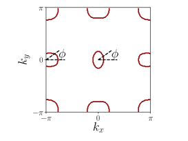
Figure 1: Calculated Fermi surface in the nematic normal phase of FeSe with $\eta=0.07$ and $\lambda=-0.03$.

Nematic order.  In the nematic phase, the breaking of $C_{4}$ symmetry induces additional anisotropies to both the kinetic energy and exchange interactions. To take this effect into account in a simple way, we introduce an anisotropy parameter $\eta$ in the nearest-neighbor hopping parameters and the exchange couplings of the $d_{xz/yz}$ orbitals as follows,

$$t_{x/y}=t(1\pm\eta);~{}~{}~{}~{}~{}~{}J_{x/y}=J(1\pm\eta)^{2}.$$ (3)

For example, the nearest-neighbor hopping terms of the $d_{xz/yz}$ orbitals contains the following in the nematic phase,

$$\eta\left[t_{1}(c_{xz,i}^{\dagger}c_{xz,i+e_{x}}-c_{yz,i}^{\dagger}c_{yz,i+e_{y}})\right.$$

$$+ \left.t_{2}(-c_{xz,i}^{\dagger}c_{xz,i+e_{y}}+c_{yz,i}^{\dagger}c_{yz,i+e_{x}})\right].$$

The latter corresponds to a combination of the $s$- and $d$-wave bond nematic orders bond_nematic_waston ,

$$\eta\left[\frac{t_{1}-t_{2}}{2}(\cos(k_{x})+\cos(k_{y}))(n_{xz,k}-n_{yz,k})\right.$$

$$\left.+\frac{t_{1}+t_{2}}{2}(\cos(k_{x})-\cos(k_{y}))(n_{xz,k}+n_{yz,k})\right].$$

Fermi surface in the nematic phase.  We use the notation of the 1-Fe Brillouin zone (BZ). In Fig. 1, we show the Fermi surface in the nematic phase for $\eta=0.07$. An atomic spin-orbit coupling (SOC), of the form $\lambda\textbf{S}\cdot\textbf{L}$, is included in the calculation for Fig. 1. The superconductivity considered here is mainly driven by the magnetic interactions. Because the SOC is much smaller than the magnetic bandwidth, its effect on the pairing will be neglected. With increasing $\eta$, the inner hole pocket near the $\Gamma$ point quickly disappears; this evolution is shown in Fig.S1 of the SM suppl . The (outer) hole pocket near the $\Gamma$ point is elongated along the $k_{y}$ direction. The electron pocket near the $M_{x}$ [$(\pi,0)$] point is also elongated, along the $k_{x}$ direction. The electron pocket is dominated by the $d_{yz}$ and $d_{xy}$ orbitals, whereas the hole pocket mainly comprises the $d_{xz}$ and $d_{yz}$ orbitals (Fig. S2 suppl ). The hole pocket near the $(\pi,\pi)$ point, which appears in our model as a result of the known artifact of the DFT calculations dft2008 ; dft2010 ; dft_jpsj , does not come into play in our main result.

pairing channel	$D_{4h}$	$D_{2h}$	pairing channel in real space
$s_{x^{2}+y^{2}}\ \tau_{0}$	$A_{1g}$	$A_{g}$	${\sum}_{\textbf{e}\in\{e_{x},e_{y}\}}\bigg{(}\Delta_{xz}(\textbf{e})+\Delta_{yz}(\textbf{e})\bigg{)}$
$s_{x^{2}y^{2}}\ \tau_{0}$	$A_{1g}$	$A_{g}$	${\sum}_{\textbf{e}\in\{e_{x}\pm e_{y}\}}\bigg{(}\Delta_{xz}(\textbf{e})+\Delta_{yz}(\textbf{e})\bigg{)}$
$s_{x^{2}y^{2}}\ \tau_{z}$	$B_{1g}$	$A_{g}$	${\sum}_{\textbf{e}\in\{e_{x}\pm e_{y}\}}\bigg{(}\Delta_{xz}(\textbf{e})-\Delta_{yz}(\textbf{e})\bigg{)}$
$d_{x^{2}-y^{2}}\ \tau_{0}$	$B_{1g}$	$A_{g}$	${\sum}_{\alpha\in\{xz,yz\}}\bigg{(}\Delta_{\alpha}(e_{x})-\Delta_{\alpha}(e_{y})\bigg{)}$

Table 1: Symmetry classification of spin-singlet intra-orbital pairing channels by the $D_{4h}$ and $D_{2h}$ point groups. Here, $\tau_{i}$ are the Pauli matrices in the $d_{xz},d_{yz}$ orbital basis. A complete list involving these orbitals and the $d_{xy}$ orbital is given in the SM suppl

.

Pairing structure in the nematic phase.  We next analyze the influence of nematic order on the pairing structure. The pairing can be classified by the irreducible representations of the point group associated with the lattice symmetry, which is summarized in Table  1 and in the SM suppl . In the tetragonal phase, the corresponding point group is $D_{4h}$. For example, the usual $s$-wave and $d$-wave pairings have an $A_{1g}$ and a $B_{1g}$ symmetry, respectively. In the nematic phase, the point group is reduced to $D_{2h}$. In this case, both the $A_{1g}$ and $B_{1g}$ representations of $D_{4h}$ belong to the $A_{g}$ representation of the $D_{2h}$ group. As a consequence, the $s$- and $d$-wave pairing channels will generically mix.

We now turn to detailed calculations. Because the relevant electronic states are dominated by the $d_{xz}$,$d_{yz}$,and $d_{xy}$ orbitals, we only consider the nearest-neighbor and next-nearest-neighbor intraorbital exchange interactions for these three orbitals. As in the previous study of orbital-selective pairing in the tetragonal phase osp_nica , we introduce two ratios $r_{L}$ and $r_{O}$. Here, $r_{L}=\frac{J_{1}}{J_{2}}$, for each orbital, quantifies the magnetic frustration effect; $r_{O}=\frac{J_{2}^{xy}}{J_{2}^{xz/yz}}=\frac{J_{1}^{xy}}{J_{1}^{xz/yz}}$ reflects the orbital-selective effect between the $xz/yz$ and $xy$ orbitals. (The inter-orbital pairings are negligibly small osp_nica .)

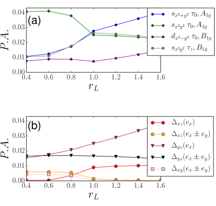
Figure 2: (Color online) Top panel: Evolution of the pairing amplitudes (P.A.), $\Delta$, with magnetic frustration parameter $r_{L}$ for several channels according to the $D_{4h}$ representations. The parameters are $\eta=0.07$, $r_{O}=0.3$, and $J_{2,xz/yz}=0.3$. Bottom panel: Same as the top panel but shown according to the $D_{2h}$ representations, demonstrating a strong orbital-selective pairing with $\Delta_{yz}\gg\Delta_{xz/xy}$.

In Fig. 2, we present the evolution of the pairing amplitudes of several pairing channels with $r_{L}$. The top panel shows the pairing channels classified by the $D_{4h}$ group. The dominant pairing always has an $A_{1g}$ symmetry. With increasing $r_{L}$, it crosses over from the sign-changing $s$ wave (with form factor $\cos k_{x}\cos k_{y}$) to an extended $s$-wave (with form factor $\cos k_{x}+\cos k_{y}$). It is more transparent to show the pairing amplitudes according to the irreducible representations of the $D_{2h}$ group. As illustrated in the bottom panel of Fig. 2, we find strong orbital-selective pairing with $|\Delta_{yz}|/|\Delta_{xz/xy}|>2$. Such an orbital-selective pairing is quite robust within a wide range of $r_{L}$ and $r_{O}$ values.

The strong orbital selectivity in the superconducting pairing is connected with that of the normal state. To see this, note that from Eq. (2) we have the ratio of the pairing amplitudes,

$$\frac{|\Delta_{yz}|}{|\Delta_{xz/xy}|}=\frac{Z_{yz}}{Z_{xz/xy}}\frac{|\tilde{\Delta}_{yz}|}{|\tilde{\Delta}_{xz/xy}|}.$$ (4)

In other words, the orbital selectivity of the pairing amplitudes is magnified by $\frac{Z_{yz}}{Z_{xz/xy}}$, the ratio of the quasiparticle spectral weights in the normal state.

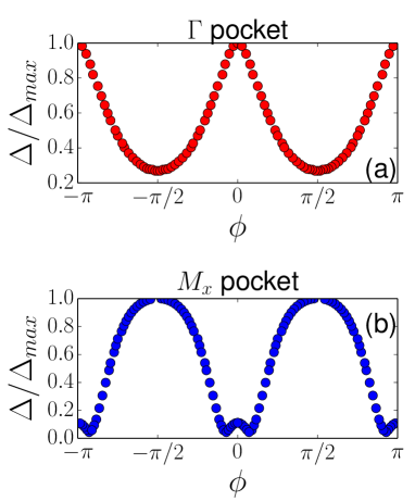
Figure 3: Top: Variation of the superconducting gap on the hole (top panel) and electron (bottom panel) pockets near $\Gamma$ and $M_{x}$ points of the BZ, respectively. The angle $\phi$ is defined as in Fig. 1. Along each pocket, the gap values are normalized by the corresponding maximum. The calculations are for $r_{L}=1.2$, $r_{O}=0.3$, and $\eta=0.07$.

Gap anisotropy.  We now calculate the superconducting gap on the normal-state Fermi surface. In Fig. 3 we plot the gap variation on the hole (near $\Gamma$) and electron (near $M_{x}$) Fermi pockets. Along each Fermi pocket, the gap values are normalized by its corresponding maximal value, and the angle $\phi$ is defined in Fig. 1. For the Fermi pocket near $\Gamma$, the gap maximum appears at $\phi=0/\pi$ and the minimum is at $\phi=\frac{\pi}{2}$. For the pocket near $M_{x}$, the maximum is at $\phi=\frac{\pi}{2}$ and the minimum is close to $\phi=0$. These positions of the gap maximum/minimum, as well as the large gap anisotropy on both Fermi pockets, are consistent with the experimental results stm . More specifically, i) the ratio of the maximum gap of the hole pocket to that of the electron pocket is of order unity, about $1.01$ in our calculation. Experimentally, the ratio is comparable to this: It is $1.5$ ($1.0$) when the maximal gap on the hole pocket is inferred from the STM stm (laser-ARPES Shin-FeSe ) measurements. ii) The calculated ratio of the gap minimum to gap maximum for the electron pocket ($\sim 5\%$) is comparable to its experimental counterpart (in the range 5%-30%) stm . iii) Likewise, the calculated ratio for the hole pocket ($\sim 25\%$) is comparable to its experimental counterpart (4%-25%) stm .

Our results are understood as follows. At any given point of the Fermi surface k, the overall gap $\Delta(\textbf{k})=\sum\Delta_{\alpha}(\textbf{k})W_{\alpha}(\textbf{k})$. Here, $W_{\alpha}$ is the orbital weight, and $\Delta_{\alpha}(\textbf{k})=\sum_{\textbf{e}\in\{e_{x},e_{y},e_{x}\pm e_{y}\}}J_{\textbf{e}}^{\alpha\alpha}\Delta_{\alpha}(\textbf{e})\cos(\textbf{k}\cdot\textbf{e})$ is the orbital-resolved gap. As an illustration, we show the distributions of the orbital-resolved gap and the corresponding orbital weight on the electron pocket near $M_{x}$ in Fig. 4 (and for the hole pocket in the SM suppl ). Along the electron pocket, near $\phi=\frac{\pi}{2}$, the $yz$ orbital has the largest orbital weight. Thus, the gap there is dominated by the pairing in the $yz$ orbital, namely, $\Delta({\phi=\frac{\pi}{2}})\approx\Delta_{yz}$. Similarly, near $\phi=0$, the $xy$ orbital has the largest orbital weight and then $\Delta({\phi=0})\approx\Delta_{xy}$. The strong orbital-selectivity in the pairing amplitude $|\Delta_{yz}(\textbf{e})|\gg|\Delta_{xy}(\textbf{e})|$ gives rise to a large gap anisotropy $|\Delta({\phi=\frac{\pi}{2}})|\approx|\Delta_{yz}|\gg|\Delta_{xy}|\approx|\Delta({\phi=\frac{\pi}{2}})|$. A similar argument applies to the hole pocket, where $|\Delta({\phi=0})|\approx|\Delta_{yz}|\gg|\Delta_{xz}|\approx|\Delta({\phi=\frac{\pi}{2}})|$, as seen in the SMsuppl .

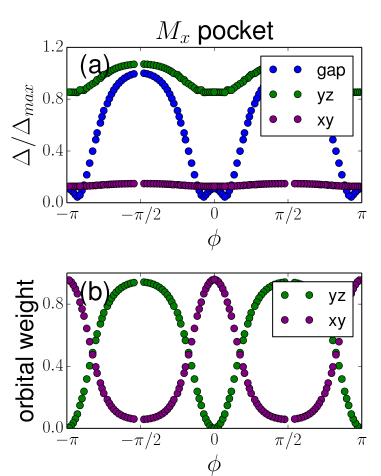
Figure 4: (Color online) (Top): Overall and orbital resolved superconducting gaps along the $M_{x}$ electron pocket. (Bottom): Weight distributions of the $xy$ and $yz$ orbitals along the $M_{x}$ electron pocket.

Discussions.  In principle, additional factors may influence the gap anisotropy. For instance, it has been shown that the magnetic frustration $r_{L}$ can tune the relative strength of nearest-neighbor and next nearest-neighbor pairings, and gives rise to a moderate level of gap anisotropy along the electron pocket in NaFeAs Yu_PRB2014 . For FeSe, we have focused on the regime $r_{L}\sim 1$: The absence of antiferromagnetic order in the nematic state suggests a strong magnetic frustration with $r_{L}\sim 1$, where the nearest-neighbor and next nearest-neighbor pairings are quasidegenerate.

In the calculations we have carried out, the nematicity has multiple effects on the pairing structure. First, it enhances the orbital selectivity in the spectral weight of the coherent itinerant electrons, leading to strong orbital-selective pairing amplitudes, as shown in Eq. (4). Second, the orbital weights are largely redistributed along the distorted Fermi surface as a combined effect of the additional anisotropy and orbital-dependent band-structure renormalization in the nematic phase. On each Fermi pocket, the dominant orbital character has a large variation. Third, the nematicity induces additional magnetic anisotropy, which enhances the pairing in the $e_{x}$ direction but reduces the pairing in the $e_{y}$ direction. While this last effect also contributes to the gap anisotropy, it is not the dominant source in our case. In other words, the gap anisotropy primarily originates from the first two effects, which dictate the orbital-selective nature of the pairing amplitudes.

The orbital-selective pairing concerns superconductivity driven by short-range spin-exchange interactions between the electrons associated with the multiple $3d$ orbitals. For FeSe, direct evidence exists that the local Coulomb (Hubbard and Hund’s) interactions are strong Watson2017 ; Evtushinksy , and the orbitals thus represent a natural basis to consider superconducting pairing.

We now discuss the broader implications of the orbital selective pairing. There is accumulating evidence that superconductivity in the FeSCs is mainly driven by magnetic correlations. Yet, the precise role of the nematicity on the superconductivity remains an open question. Our study raises the possibility that the main influence of the nematicity on the magnetically driven superconductivity is through its influence on the orbital selectivity.

Finally, the correlation effects provide intuition on how to control low-energy physics by tuning local degrees of freedom. For instance, the multi-orbital nature affords a handle for engineering the low-energy electronic states and raising $T_{c}$. Even when the superconductivity is primarily driven by magnetic correlations, tuning the orbital levels and orbital-dependent couplings may optimize superconductivity. This notion is consistent with experiments on single-layer FeSe XShi , which indicate a further increased $T_{c}$ by varying the weight of particular $3d$ orbitals near the Fermi energy.

Conclusions.  We have studied the superconductivity in the nematic phase of FeSe through a multiorbital model using a $U(1)$ slave-spin approach. The enhanced orbital selectivity in the normal state by the nematic order is shown to yield a strong orbital-selective superconducting pairing. The latter produces sizable gap anisotropy on both the hole and electron pockets, which naturally explains the recent experimental observations. The orbital-selective pairing raises the prospect of harnessing the orbital degrees of freedom to realize still higher $T_{c}$, even when superconductivity is magnetically driven, and provides insights into the interplay between electronic orders and superconductivity. As such, our results shed light not only on the physics of the iron-based compounds but also on the unconventional superconductivity in a variety of other strongly correlated systems.

I Supplemental Material

I.1 Details on the Model and Self-consistent Calculations of the Pairing Amplitudes

We consider a five-orbital Hubbard model for FeSe. The Hamiltonian reads as

$$H = H_{t}+H_{\rm{int}},$$

$$H_{t} = \sum_{ij,\alpha\beta}t_{ij}^{\alpha\beta}c_{i,\alpha,\sigma}^{\dagger}c_{j,\beta,\sigma},$$

$$H_{\rm{int}} = \frac{U}{2}\sum_{i,\alpha,\sigma}n_{i\alpha\sigma}n_{i\alpha\bar{\sigma}}+\sum_{i,\alpha<\beta,\sigma}\left\{U^{\prime}n_{i\alpha\sigma}n_{i\beta\bar{\sigma}}\right.+(U^{\prime}-J_{\rm{H}})n_{i\alpha\sigma}n_{i\beta\sigma}$$ (5)

$$\left.-J_{\rm{H}}(c^{\dagger}_{i\alpha\sigma}c_{i\alpha\bar{\sigma}}c^{\dagger}_{i\beta\bar{\sigma}}c_{i\beta\sigma}+c^{\dagger}_{i\alpha\sigma}c^{\dagger}_{i\alpha\bar{\sigma}}c_{i\beta\sigma}c_{i\beta\bar{\sigma}})\right\},$$

where $c_{i,\alpha,\sigma}^{\dagger}$ creates an electron in orbital $\alpha(\in{xz,yz,x^{2}-y^{2},xy,z^{2}})$, spin $\sigma$ and at site $i$ of an Fe-square lattice, and $H_{\rm{int}}$ describes the on-site interactions, which include the intra- and inter-orbital Coulomb repulsions $U$ and $U^{\prime}$, and the Hund’s coupling $J_{\rm{H}}$. After integrating out the incoherent part of the electron spectrum via the $U(1)$ slave-spin approach, we obtain an effective multi-orbital $t$-$J$ model. In terms of the $f$-fermions this effective model takes the following form:

$$H_{eff} = \sum_{ij,\alpha\beta}\widetilde{t}_{ij}^{\alpha\beta}f_{i,\alpha,\sigma}^{\dagger}f_{j,\beta,\sigma}-\sum_{ij,\alpha\beta}J_{ij}^{\alpha\beta}f_{j,\beta,\downarrow}^{\dagger}f_{i,\alpha,\uparrow}^{\dagger}f_{i,\alpha,\downarrow}f_{j,\beta,\downarrow}$$ (6)

with the normalized hopping term $\widetilde{t}_{ij}^{\alpha\beta}=\sqrt{Z_{\alpha}Z_{\beta}}t_{ij}^{\alpha\beta}-\lambda_{\alpha}\delta_{\alpha\beta}\delta_{ij}$. Here we only consider the intraorbital exchange interaction with $J^{\alpha\beta}=J^{\alpha}\delta_{\alpha\beta}$.

We consider the pairing amplitudes of the $f$-fermions,

$$\widetilde{\Delta}_{\textbf{e},\alpha}=\frac{1}{2N}\sum_{i}\bigg{<}f_{i,\alpha,\uparrow}f_{i+\textbf{e},\alpha,\downarrow}-f_{i,\alpha,\downarrow}f_{i+\textbf{e},\alpha,\uparrow}\bigg{>}$$ (7)

where $\textbf{e}\in\{e_{x},e_{y},e_{x+y},e_{x-y}\}$. From a Hubbard-Stratonovich decoupling, the $H_{eff}$ is reduced into fermion bilinears and $\widetilde{\Delta}_{\textbf{e},\alpha}$ can then be solved. The pairing amplitude of the physical electrons is obtained as follows:

$${\Delta}_{\textbf{e},\alpha}=\frac{1}{2N}\sum_{i}\bigg{<}c_{i,\alpha,\uparrow}c_{i+\textbf{e},\alpha,\downarrow}-c_{i,\alpha,\downarrow}c_{i+\textbf{e},\alpha,\uparrow}\bigg{>}=Z_{\alpha}\widetilde{\Delta}_{\textbf{e},\alpha}$$ (8)

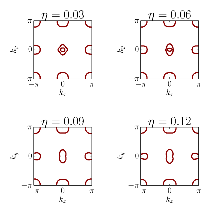
Figure S1: (Color online) Evolution of the Fermi surface with the anisotropy parameter $\eta$ in the nematic phase.

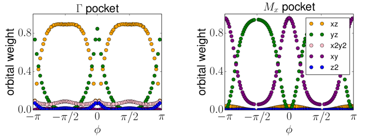
Figure S2: (Color online) Orbital weights along the outer hole pocket near $\Gamma$ (left panel) and those for the electron pocket near M_x (right panel).

I.2 Details on the tight-binding parameters

We present the tight-binding parameters in Table S1. To obtain the tight-binding parameters, we perform local density approximation (LDA) calculations for bulk FeSe with a tetragonal structure, and we fit the LDA band structure to the tight-binding Hamiltonian. The form of the five-orbital tight-binding Hamiltonian given in Ref. [SM_Graser_2009, ] is used.

	$\alpha=1$	$\alpha=2$	$\alpha=3$	$\alpha=4$	$\alpha=5$
$\epsilon_{\alpha}$	-0.00733	-0.00733	-0.52154	0.10974	-0.5694
$t^{\alpha\alpha}_{\mu}$	$\mu=x$	$\mu=y$	$\mu=xy$	$\mu=xx$	$\mu=xxy$	$\mu=xyy$	$\mu=xxyy$
$\alpha=1$	-0.0111	-0.49155	-0.23486	-0.0119	-0.04025	-0.03917	-0.03808
$\alpha=3$	-0.38485		-0.08015	-0.00646
$\alpha=4$	-0.16872		-0.10728	-0.00626	-0.04592		-0.02079
$\alpha=5$	-0.03681			-0.00159	-0.01585		-0.02739
$t^{\alpha\beta}_{\mu}$	$\mu=x$	$\mu=xy$	$\mu=xxy$	$\mu=xxyy$
$\alpha\beta=12$		-0.12701	-0.00655	-0.05869
$\alpha\beta=13$	-0.36123	-0.07201	-0.0134
$\alpha\beta=14$	-0.20068	-0.03548	-0.00705
$\alpha\beta=15$	-0.08057	-0.14823		-0.01218
$\alpha\beta=34$			-0.0217
$\alpha\beta=35$	-0.29868		-0.01332
$\alpha\beta=45$		-0.13208		-0.05213

Supplemental Table S1. Tight-binding parameters of the five-orbital model for bulk FeSe with the tetragonal structure. Here we use the same notation as in Ref.  [SM_Graser_2009, ]. The orbital index $\alpha=$1,2,3,4,5 correspond to $d_{xz}$, $d_{yz}$, $d_{x^{2}-y^{2}}$, $d_{xy}$, and $d_{3z^{2}-r^{2}}$ orbitals, respectively. The listed parameters are in eV.

I.3 Evolution of the Fermi surface

To study the effect of nematic order on the Fermi surface, we set the interaction strength to zero and calculate the Fermi surface and orbital weight distribution of the tight-binding model with various nematic order parameters. In Fig. S1, we show the evolution of the Fermi surface with the anisotropy parameter $\eta$. The $\Gamma$ pocket enlarges in the $y$ direction and both $\Gamma$ and M_x pockets have a peanut shape for sufficiently large $\eta$. In Fig. S2, we plot the orbital weight distribution at $\eta=0.07$. The $\Gamma$ pocket is dominated by the $d_{xz}$ and $d_{yz}$ orbitals and the M_x pocket by the $d_{yz}$ and $d_{xy}$ orbitals.

I.4 Classification of the Pairing Channels

The pairing channels can be classified by using the irreducible representations of the lattice point group of the system. For the tetragonal symmetry, the corresponding lattice point group is $D_{4h}$. In the presence of the nematic order, the $C_{4}$ rotational symmetry is broken, and the point group is reduced to $D_{2h}$. In the main text, we consider the intraorbital spin-singlet pairing channels of the system. A full list of these pairing channels involving the $d_{xz}$, $d_{yz}$, and $d_{xy}$ orbitals and their corresponding symmetry classification are given in Table S2.

pairing channel in momentum space	$D_{4h}$	$D_{2h}$	pairing channel in real space
$s_{x^{2}+y^{2}}\tau_{0}$	$A_{1g}$	$A_{g}$	$\Delta_{xz}(e_{x})+\Delta_{xz}(e_{y})+\Delta_{yz}(e_{x})+\Delta_{yz}(e_{y})$
$s_{x^{2}y^{2}}\tau_{0}$	$A_{1g}$	$A_{g}$	$\Delta_{xz}(e_{x}+e_{y})+\Delta_{xz}(e_{x}-e_{y})+\Delta_{yz}(e_{x}+e_{y})+\Delta_{yz}(e_{x}-e_{y})$
$d_{x^{2}-y^{2}}\tau_{z}$	$A_{1g}$	$A_{g}$	$\Delta_{xz}(e_{x})-\Delta_{xz}(e_{y})-\Delta_{yz}(e_{x})+\Delta_{yz}(e_{y})$
$d_{x^{2}-y^{2}}\tau_{0}$	$B_{1g}$	$A_{g}$	$\Delta_{xz}(e_{x})-\Delta_{xz}(e_{y})+\Delta_{yz}(e_{x})-\Delta_{yz}(e_{y})$
$s_{x^{2}+y^{2}}\tau_{z}$	$B_{1g}$	$A_{g}$	$\Delta_{xz}(e_{x})+\Delta_{xz}(e_{y})-\Delta_{yz}(e_{x})-\Delta_{yz}(e_{y})$
$s_{x^{2}y^{2}}\tau_{z}$	$B_{1g}$	$A_{g}$	$\Delta_{xz}(e_{x}+e_{y})+\Delta_{xz}(e_{x}-e_{y})-\Delta_{yz}(e_{x}+e_{y})-\Delta_{yz}(e_{x}-e_{y})$
$d_{xy}\tau_{z}$	$A_{2g}$	$B_{1g}$	$\Delta_{xz}(e_{x}+e_{y})-\Delta_{xz}(e_{x}-e_{y})-\Delta_{yz}(e_{x}+e_{y})+\Delta_{yz}(e_{x}-e_{y})$
$d_{xy}\tau_{0}$	$B_{2g}$	$B_{1g}$	$\Delta_{xz}(e_{x}+e_{y})-\Delta_{xz}(e_{x}-e_{y})+\Delta_{yz}(e_{x}+e_{y})-\Delta_{yz}(e_{x}-e_{y})$
$s_{x^{2}y^{2}}\mathds{1}_{xy}$	$A_{1g}$	$A_{g}$	$\Delta_{xy}(e_{x}+e_{y})+\Delta_{xy}(e_{x}-e_{y})$
$s_{x^{2}+y^{2}}\mathds{1}_{xy}$	$A_{1g}$	$A_{g}$	$\Delta_{xy}(e_{x})+\Delta_{xy}(e_{y})$
$d_{x^{2}-y^{2}}\mathds{1}_{xy}$	$B_{1g}$	$A_{g}$	$\Delta_{xy}(e_{x})-\Delta_{xy}(e_{y})$
$d_{xy}\mathds{1}_{xy}$	$B_{2g}$	$B_{1g}$	$\Delta_{xy}(e_{x}+e_{y})-\Delta_{xy}(e_{x}-e_{y})$

Table S2. Symmetry classification of the spin-singlet intra-orbital pairing channels involving the $d_{xz},d_{yz},d_{xy}$ orbitals. Here $\tau_{i}$ are the Pauli matrices of the isospin operator in the $d_{xz/yz}$ orbital basis.

I.5 Phase Diagram and the Pairing Amplitude

To study the evolution of pairing symmetry in the nematic phase, we fix $\eta=0.07$ and solve for the pairing amplitudes at different $r_{L}$ and $r_{O}$ values. Fig. S3 is the resulting phase diagram where each regime is characterized by the leading pairing channel. Fig. S4 and Fig. S5 show the evolution of pairing amplitude with $r_{L}$ at $r_{O}=0.3$. As is seen, the pairing amplitude in the $d_{yz}$ orbital is always larger than those of the $d_{xz}$ and $d_{xy}$ orbitals. In addition, the pairing in $e_{x}$ direction is dominant when $r_{L}$ is small and the pairing in $e_{x\pm y}$ direction is dominant when $r_{L}$ is large.

Figure S3: (Color online) Phase diagram showing the different regimes with different leading pairing channels in the $r_{L}$-$r_{O}$ plane.

Figure S4: (Color online) Pairing amplitudes in the different channels according to the irreducible representations of the $D_{4h}$ group.

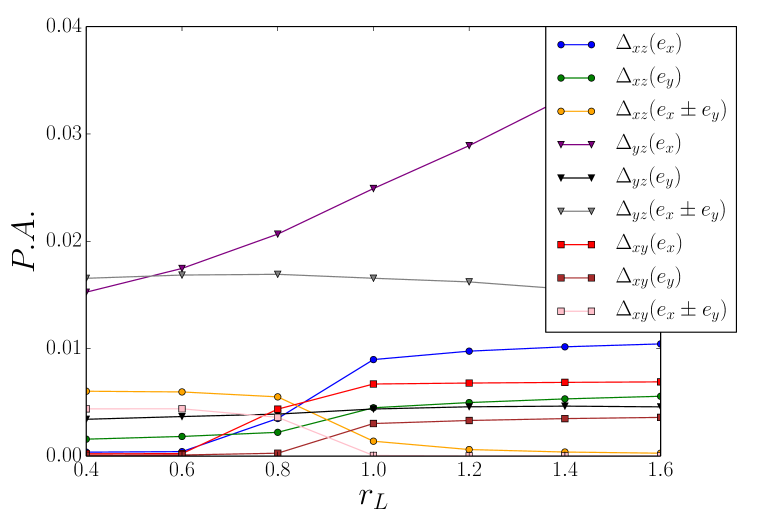
Figure S5: (Color online) Pairing amplitudes of the different orbitals expressed in the irreducible representations of the $D_{2h}$ group.

I.6 Gap anisotropy along the $\Gamma$ pocket

In Fig. S6 (top panel), we show the gap anisotropy and the paring strength of the $d_{xz}$ and $d_{yz}$ orbitals along the $\Gamma$ hole pocket. In Fig. S6 (bottom panel), we plot the weight distributions of the $d_{xz}$ and $d_{yz}$ orbitals along the same pocket. At $\phi=0$, the $yz$ orbital has the largest orbital weight, and $\Delta({\phi=0})\sim{\Delta}_{yz}$. At $\phi=\frac{\pi}{2}$, the $xz$ orbital has the largest orbital weight; correspondingly, $\Delta({\phi=\frac{\pi}{2}})\sim\Delta_{xz}$. For strong orbital selective pairing, $\Delta_{yz}\gg\Delta_{xz}$. As a result, the gap will become very anisotropic with $\Delta({\phi=0})\gg\Delta({\phi=\frac{\pi}{2}})$.

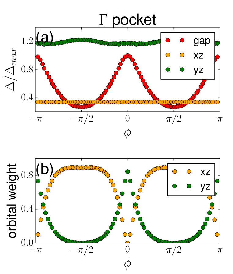
Figure S6: (Color online) Gap anisotropy and orbital weight distribution of the $\Gamma$ pocket

References

- (1) S. Graser et al., New J. Phys. 11, 025016 (2009).