Nonparametric Bayesian volatility learning under microstructure noise

Abstract.

Aiming at financial applications, we study the problem of learning the volatility under market microstructure noise. Specifically, we consider noisy discrete time observations from a stochastic differential equation and develop a novel computational method to learn the diffusion coefficient of the equation. We take a nonparametric Bayesian approach, where we model the volatility function a priori as piecewise constant. Its prior is specified via the inverse Gamma Markov chain. Sampling from the posterior is accomplished by incorporating the Forward Filtering Backward Simulation algorithm in the Gibbs sampler. Good performance of the method is demonstrated on two representative synthetic data examples. Finally, we apply the method on the EUR/USD exchange rate dataset.

1. Introduction

Let the one-dimensional stochastic differential equation (SDE)

(1) $${{\mathrm{d}}}X_{t}=b(t,X_{t})\,{{\mathrm{d}}}t+s(t)\,{{\mathrm{d}}}W_{t},\quad X_{0}=x_{0},\quad t\in[0,T],$$

be given. Here $W$ is a standard Wiener process and $b$ and $s$ are referred to as the drift function and volatility function respectively. We assume (not necessarily uniformly spaced) observation times $\{t_{i}:1\leq i\leq n\}$ and observations $\mathcal{Y}_{n}=\{Y_{1},\ldots,Y_{n}\},$ where

(2) $$Y_{i}=X_{t_{i}}+V_{i},\quad 0<t_{1}<\cdots<t_{n}=T,$$

and $\{V_{i}\}$ is a sequence of independent and identically distributed random variables, independent of $W$. Our aim is to nonparametrically learn the volatility $s$ using the noisy observations $\scr{Y}_{n}$. Knowledge of the volatility is of paramount importance in financial applications, specifically in pricing financial derivatives, see, e.g., Musiela and Rutkowski (2005), and in risk management.

The quantity $\Delta t_{i}=t_{i}-t_{i-1}$ is referred to as the observation frequency; small values of $\Delta t_{i}$ correspond to high frequency, dense-in-time data. Intraday financial data are commonly thought to be high frequency data. In this high frequency financial data setting, which is the one we are interested in in this work, the measurement errors $\{V_{i}\}$ are referred to as microstructure noise. Their inclusion in the model aims to reflect such features of observed financial time series as their discreteness or approximations due to market friction. Whereas for low-frequency financial data these can typically be neglected without much ensuing harm, empirical evidence shows that this is not the case for high frequency data; cf. Mykland and Zhang (2012).

There exists a large body of statistics and econometrics literature on nonparametric volatility estimation under microstructure noise. See, e.g., Hoffmann et al. (2012), Jacod et al. (2009), Mykland and Zhang (2009), Reiß (2011), Sabel et al. (2015); a recent overview is Mykland and Zhang (2012). The literature predominantly deals with estimation of the integrated volatility $\int_{0}^{t}s^{2}(u){{\mathrm{d}}}u$, although inference on $s$ has also been studied in several of these references. Various methods proposed in the above-mentioned works share the property of being frequentist in nature.

In this paper, our main and novel contribution is the development of a practical nonparametric Bayesian approach to volatility learning under microstructure noise. More specifically, we propose a novel Bayesian approach to volatility learning and demonstrate good performance of our method on two representative simulation examples. We also apply our method on the EUR/USD exchange rate dataset.

In general, a nonparametric approach reduces the risk of model misspecification; the latter may lead to distorted inferential conclusions. The presented nonparametric method is not only useful for an exploratory analysis of the problem at hand (cf. Silverman (1986)), but also allows honest representation of inferential uncertainties (cf. Müller and Mitra (2013)). Attractive features of the Bayesian approach include its internal coherence, automatic uncertainty quantification in parameter estimates via Bayesian credible sets, and the fact that it is a fundamentally likelihood-based method. For a modern monographic treatment of nonparametric Bayesian statistics see Ghosal and van der Vaart (2017); an applied perspective is found in Müller et al. (2015).

The paper is organised as follows: in Section 2 we introduce in detail our approach. In Section 3 we test its practical performance on synthetic data examples. Section 4 applies our method on a real data example. Section 5 summarises our findings. Finally, Appendices A, B, C and D contain the frequently used notation and give further implementational details.

2. Methodology

In this section we introduce our methodology for inferring the volatility. We first recast the model into a simpler form amenable to computational analysis, next specify a nonparametric prior on the volatility, and finally describe an MCMC method for sampling from the posterior.

2.1. Linear state space model

Let $t_{0}=0$. By equation (1), we have

(3) $$X_{t_{i}}=X_{t_{i-1}}+\int_{t_{i-1}}^{t_{i}}b(t,X_{t}){{\mathrm{d}}}t+\int_{t_{i-1}}^{t_{i}}s(t){{\mathrm{d}}}W_{t}.$$

We derive our method under the assumption that the “true”, data-generating volatility $s$ is a deterministic function of time $t$. Next, if the “true” $s$ is in fact a stochastic process, we apply our procedure without further changes, as if $s$ were deterministic. As shown in the example of Subsection 3.2, this works in practice.

Over short time intervals $[{t_{i-1}},{t_{i}}]$, the term $\int_{t_{i-1}}^{t_{i}}s(t){{\mathrm{d}}}W_{t}$ in (3), roughly speaking, will dominate the term $\int_{t_{i-1}}^{t_{i}}b(t,X_{t}){{\mathrm{d}}}t$, as the former scales as $\Delta t_{i}$, whereas the latter as $\sqrt{\Delta t_{i}}$ (due to the properties of the Wiener process paths). As our emphasis is on learning $s$ rather than $b$, following Gugushvili et al. (2017), Gugushvili et al. (2018a) we act as if the process $X$ had a zero drift, $b\equiv 0$. A similar idea is often used in frequentist volatility estimation procedures in the high frequency financial data setting; see Mykland and Zhang (2012), Section 2.1.5 for an intuitive exposition. Formal results why this works in specific settings rely on Girsanov’s theorem, see, e.g., Hoffmann et al. (2012), Mykland and Zhang (2009), Gugushvili et al. (2017). Further reasons why one would like to set $b=0$ are that $b$ is a nuisance parameter, in specific applications its appropriate parametric form might be unknown, and finally, the observed time series might simply be not long enough to learn $b$ consistently (see Ignatieva and Platen (2012)).

We thus assume $X_{t_{i}}=X_{t_{i-1}}+U_{i},$ where $U_{i}=\int_{t_{i-1}}^{t_{i}}s(t){{\mathrm{d}}}W_{t}.$ Note that then

(4) $$U_{i}\sim N(0,w_{i})\quad\text{with}\quad w_{i}=\int_{t_{i-1}}^{t_{i}}s^{2}(t){{\mathrm{d}}}t,$$

and also that $\{U_{i}\}$ is a sequence of independent random variables. To simplify our notation, write $x_{i}=X_{t_{i}}$, $y_{i}=Y_{i}$, $u_{i}=U_{i}$, $v_{i}=V_{i}$. The preceding arguments and (2) allow us to reduce our model to the linear state space model

(5) $$\begin{split}x_{i}&=x_{i-1}+u_{i},\\ y_{i}&=x_{i}+v_{i},\end{split}$$

where $i=1,\dots,n$. The first equation in (5) is the state equation, while the second equation is the observation equation. We assume that $\{v_{i}\}$ is a sequence of independent $N(0,\eta_{v})$ distributed random variables, independent of the Wiener process $W$ in (1), so that $\{v_{i}\}$ is independent of $\{u_{i}\}$. For justification of such assumptions on the noise sequence $\{v_{i}\}$ from a practical point of view, see Sabel et al. (2015), page 229. We endow the initial state $x_{0}$ with the $N(\mu_{0},C_{0})$ prior distribution. Under our assumptions, (5) is a Gaussian linear state space model. This is very convenient computationally and had we not followed this route, we would have had to deal with an intractable likelihood, which constitutes the main computational bottleneck for Bayesian inference in SDE models; see, e.g, van der Meulen and Schauer (2017) and Papaspiliopoulos et al. (2013) for discussion.

2.2. Prior

For the measurement error variance $\eta_{v}$, we assume a priori $\eta_{v}\sim\operatorname{IG}(\alpha_{v},\beta_{v})$. The construction of the prior for $s$ is more complex and follows Gugushvili et al. (2018a), that in turn relies on Cemgil and Dikmen (2007). Fix an integer $m<n$. Then we have a unique decomposition $n=mN+r$ with $0\leq r<m$, where $N=\lfloor{n}/{m}\rfloor$. Now define bins $B_{k}=[t_{m(k-1)},t_{mk})$, $k=1,\ldots,N-1$, and $B_{N}=[t_{m(N-1)},T]$. We model $s$ as

(6) $$s=\sum_{k=1}^{N}\xi_{k}\mathbf{1}_{B_{k}},$$

where $N$ (the number of bins) is a hyperparameter. Then $s^{2}=\sum_{k=1}^{N}\theta_{k}\mathbf{1}_{B_{k}},$ where $\theta_{k}=\xi_{k}^{2}$. We complete the prior specification for $s$ by assigning a prior distribution to the coefficients $\theta_{1:N}$. For this purpose, we introduce auxiliary variables $\zeta_{2:N}$, and suppose the sequence $\theta_{1},\zeta_{2},\theta_{2},\ldots,\zeta_{k},\theta_{k},\ldots,\zeta_{N},\theta_{N}$ forms a Markov chain (in this order of variables). The transition distributions of this chain are defined by

(7) $$\theta_{1}\sim\operatorname{IG}(\alpha_{1},\beta_{1}),\quad\zeta_{k+1}|\theta_{k}\sim\operatorname{IG}(\alpha,\alpha\theta_{k}^{-1}),\quad\theta_{k+1}|\zeta_{k+1}\sim\operatorname{IG}(\alpha,\alpha\zeta_{k+1}^{-1}),$$

where $\alpha_{1},\beta_{1},\alpha$ are hyperparameters. We refer to this chain as an inverse Gamma Markov chain, see Cemgil and Dikmen (2007). The corresponding prior on $\theta_{1:N}$ will be called the inverse Gamma Markov chain (IGMC) prior. The definition in (7) ensures that $\theta_{1},\ldots,\theta_{N}$ are positively correlated, which imposes smoothing across different bins $B_{k}$. Simultaneously, it ensures partial conjugacy in the Gibbs sampler that we derive below, leading to simple and tractable MCMC inference. In our experience, an uninformative choice $\alpha_{1},\beta_{1}\rightarrow 0$ performs well in practice. We also endow $\alpha$ with a prior distribution and assume $\log\alpha\sim N(a,b)$, with hyperparameters $a\in\mathbb{R},b>0$ chosen so as to render the hyperprior on $\alpha$ diffuse. As explained in Gugushvili et al. (2017), Gugushvili et al. (2018a), the hyperparameter $N$ (or equivalently $m$) can be considered both as a smoothing parameter and the resolution at which one wants to learn the volatility function. Obviously, given the limited amount of data, this resolution cannot be made arbitrarily fine. On the other hand, as shown in Gugushvili et al. (2018a) (see also Gugushvili et al. (2018b)), inference with the IGMC prior is quite robust with respect to a wide range of values of $N$, as the corresponding Bayesian procedure has an additional regularisation parameter $\alpha$ that is learned from the data. Statistical optimality results in Munk and Schmidt-Hieber (2010) suggest that in our setting $N$ should be chosen considerably smaller than in the case of an SDE observed without noise (that was studied via the IGMC prior in Gugushvili et al. (2018a)).

2.3. Likelihood

Although an expression for the posterior of $s$ can be written down in closed form, it is not amenable to computations. This problem is alleviated by following a data augmentation approach, in which $x_{0:n}$ are treated as missing data; cf. Tanner and Wong (1987). An expression for the joint density of all random quantities involved is easily derived from the prior specification and (5). We have

$$p(y_{1:n},x_{0:n},\theta_{1:N},\zeta_{2:N},\alpha,\eta_{v}) =\left(\prod_{k=1}^{n}p(y_{k}\mid x_{k},\eta_{v})\right)p(x_{0:n}\mid\theta_{1:N})$$

$$\qquad p(\theta_{1})\prod_{k=1}^{N-1}\left[p(\zeta_{k+1}\mid\theta_{k},\alpha)p(\theta_{k+1}\mid\zeta_{k+1},\alpha)\right]p(\alpha).$$

Except for $p(x_{0:n}\mid\theta_{1:N})$, all the densities have been specified directly in the previous subsections. To obtain an expression for the latter, define

$$Z_{k} =\sum_{i=(k-1)m+1}^{km}\frac{(x_{i}-x_{i-1})^{2}}{\Delta_{i}},\quad k=1,\ldots,N-1,$$

$$Z_{N} =\sum_{i=(N-1)m+1}^{n}\frac{(x_{i}-x_{i-1})^{2}}{\Delta_{i}},$$

and set $m_{k}=m$ for $k=1,\ldots,N-1$, and $m_{N}=m+r$. Then

$$p(x_{0:N}\mid\theta_{1:N})\propto e^{(x_{0}-\mu_{0})^{2}/(2C_{0})}\prod_{k=1}^{N}\theta_{k}^{-m_{k}/2}\exp\left(-\frac{Z_{k}}{2\theta_{k}}\right).$$

2.4. Gibbs sampler

We use the Gibbs sampler to sample from the joint distribution of $(x_{0:n},\theta_{1:N},\zeta_{2:N},\eta_{v},\alpha)\mid y_{1:n}$. The full conditionals of $\theta_{1:N}$, $\zeta_{2:N}$, $\eta_{v}$ are easily derived from Section 2.3 and recognised to be of the inverse Gamma type. The parameter $\alpha$ can be updated via a Metropolis-Hastings step. For updating $x_{0:N}$, conditional on all other parameters, we use the standard Forward Filtering Backward Simulation (FFBS) algorithm for Gaussian state space models (cf. Section 4.4.3 in Petris et al. (2009)). The resulting Gibbs sampler is summarised in Algorithm 1. For details, see Appendix B.

Data: Observations $y_{1:n}$

Hyperparameters $\alpha_{1},$ $\beta_{1}$, $\alpha_{v}$, $\beta_{v}$, $a$, $b$, $N$;

Result: Posterior samples $\theta_{1:N}^{i}:i=1,\ldots,M$

Initialization $\theta_{1:N}^{0},$ $\zeta_{1:N}^{0}$, $\eta_{v}^{0}$, $\alpha^{0}$;

while $i\leq M$ do

       sample $x_{0:n}^{i}$ via FFBS;

       sample $\theta_{1:N}^{i}$ from the inverse Gamma full conditionals;

       sample $\zeta_{2:N}^{i}$ from the inverse Gamma full conditionals;

       sample $\eta_{v}^{i}$ from the inverse Gamma full conditional;

       sample $\alpha^{i}$ via a Metropolis-Hastings step;

       set $i=i+1$.

end while

Algorithm 1 Gibbs sampler for volatility learning

3. Synthetic data examples

In this section we study the practical performance of our method on challenging synthetic data examples. In each of them we take the time horizon $T=1$ and generate $n=4\,000$ observations as follows. First, using a fine grid of $10n+1$ time points which are sampled from the $\operatorname{Uniform}(0,1)$ distribution, conditional on including 0 and 1, a realisation of the process $X$ is obtained via Euler’s scheme. The $n$ time points $\{t_{i}\}$ are then taken as a random subsample of those times, conditional on including $1$. The settings used for the Gibbs sampler are given in Appendix C. In each example below, we plot the posterior mean and $95\%$ marginal credible band (obtained from the central posterior intervals for the coefficients $\xi_{k}=\sqrt{\theta}_{k}$ in (6)). The former gives an estimate of the volatility, while the latter provides a means for uncertainty quantification. All the computations are performed in the programming language Julia, see Bezanson et al. (2017), and we provide the code used in our examples, see Schauer and Gugushvili (2018). The hardware and software specifications for the MacBook used to perform simulations are: CPU: Intel(R) Core(TM) M-5Y31 CPU @ 0.90GHz; OS: macOS (x86_64-apple-darwin14.5.0).

3.1. Fan & Gijbels function

Suppose the volatility function is given by

(8) $$s(t)=3/2+\sin(2(4t-2))+2\exp(-16(4t-2)^{2}),\quad t\in[0,1].$$

This is a popular benchmark in nonparametric regression, which we call the Fan & Gijbels function (see Fan and Gijbels (1995)). This function was already used in the volatility estimation context in Gugushvili et al. (2017). We generated data using the drift coefficient $b(x)=-x$. For the noise level we took $\eta_{v}=0.01$, which is substantial. Given the general difficulty of learning the volatility from noisy observations, one cannot expect to infer it on a very fine resolution (cf. the remarks in Subsection 2.2), and thus we opted for $N=40$ bins.

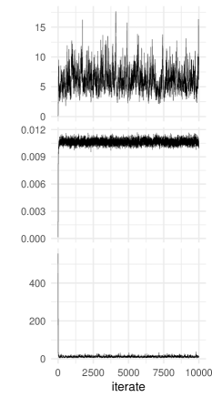
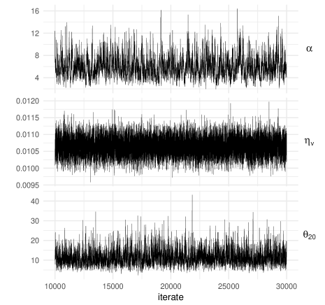
Figure 5. Trace plots for the example of Subsection 3.1. Left: first $10.000$ samples. Right: subsequent $20.000$ samples. Top: $\alpha$, middle: $\eta_{v}$, bottom: $\theta_{20}$.

Inference results are reported in Figure 1. It can be seen from the plot that we succeed in learning the volatility function. Note that the credible band does not cover the entire volatility function, but this had to be expected given that this is a marginal band. Quick mixing of the Markov chains can be visually assessed via the trace plots in Figure 5 in Appendix D. The algorithm took ca. 11 minutes to complete.

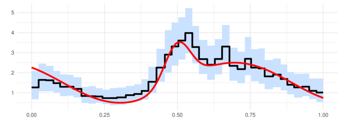
Figure 1. Posterior and pointwise $95\%$ credible band for the example of Subsection 3.1. The true volatility function is plotted in red, the black step function gives the posterior mean, and the credible band is shaded in blue.

3.2. Heston model

The Heston model (see Heston (1993)) is a widely used stochastic volatility model where it is assumed that the price process of a certain asset, denoted by $S$, evolves over time according to the SDE

$${{\mathrm{d}}}S_{t}=\mu S_{t}{{\mathrm{d}}}t+\sqrt{Z_{t}}S_{t}{{\mathrm{d}}}W_{t},$$

where the process $Z$ follows the CIR or square root process (see Cox et al. (1985)),

$${{\mathrm{d}}}Z_{t}=\kappa(\theta-Z_{t}){{\mathrm{d}}}t+\sigma\sqrt{Z_{t}}{{\mathrm{d}}}B_{t}.$$

Here $W$ and $B$ are correlated Wiener processes with correlation $\rho$. Following a usual approach in quantitative finance, we work not with $S$ directly, but with its logarithm $X_{t}=\log S_{t}$ (according to Itô’s formula it obeys a diffusion equation with volatility $s(t)=\sqrt{Z_{t}}$). We assume high-frequency observations on the log-price process $X$ with additive noise $V_{i}\sim N(0,\eta_{v})$. In this setup the volatility $s$ is a random function. We assume no further knowledge of the data generation mechanism. This setting is extremely challenging and puts our method to a serious test. To generate data, we used the parameter values $\mu=0.05,$ $\kappa=7,$ $\theta=0.04,$ $\sigma=0.6,$ $\rho=-0.6$, that mimmick the ones obtained via fitting the Heston model to real data (see Table 5.2 in van der Ploeg (2006)). Furthermore, the noise variance was taken equal to $\eta_{v}=10^{-6}.$ The latter choice ensures a sufficiently large signal-to-noise ratio in the model (5), that can be quantified via the ratio $w_{i}/\eta_{v}$ of the intrinsic noise level $w_{i}$ to the external noise level $\eta_{v}$. Finally, the parameter choice $\mu=0.04$ corresponds to a $4\%$ log-return rate, which is a reasonable value.

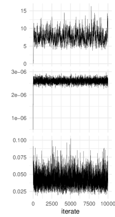
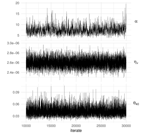
Figure 6. Trace plots for the example of subsection 3.2. Left: first $10.000$ samples. Right: subsequent $20.000$ samples. Top: $\alpha$, middle: $\eta_{v}$, bottom: $\theta_{40}$.

We report inference results with $N=80$ bins in Figure 2. These are surprisingly accurate, given a general difficulty of the problem and the amount of assumptions that went into the learning procedure. The Markov chains mix rapidly, as evidenced by the trace plots in Figure 6 in Appendix D. The simulation run took ca. 12 minutes to complete. Finally, we note that the Heston model does not formally fall into the framework under which our Bayesian method was derived (deterministic volatility function $s$). We expect that a theoretical validation why our approach also works in this case requires the use of intricate technical arguments, which lie beyond the scope of the present, practically-oriented paper.

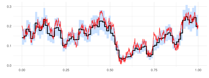
Figure 2. Posterior mean and pointwise $95\%$ credible band for the example of Subsection 3.2. The true volatility function is plotted in red, the black step function gives the posterior mean, and the credible band is shaded in blue.

4. Exchange rate data

Unlike daily stock quotes or exchange rate series that can easily be obtained via several online resources (e.g., Yahoo Finance), high frequency financial data are rarely accessible for free for academia. In this section, we apply our methodology to infer volatility of the high frequency foreign exchange rate data made available by Pepperstone Limited, the London based forex broker. Specifically, we use the EUR/USD tick data (bid prices) for 2 March 2015. As the independent additive measurement error model (2) becomes harder to justify for highly densely spaced data, we work with the subsampled data, retaining every $10$th observation; subsampling is a common strategy in this context. This results in a total of $n=13\,025$ observations over one day. As in Subsection 3.2, we apply the log-transformation on the observed time series, and assume the additive measurement error model (2). The data are displayed in Figure 3.

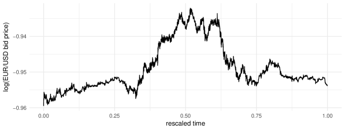
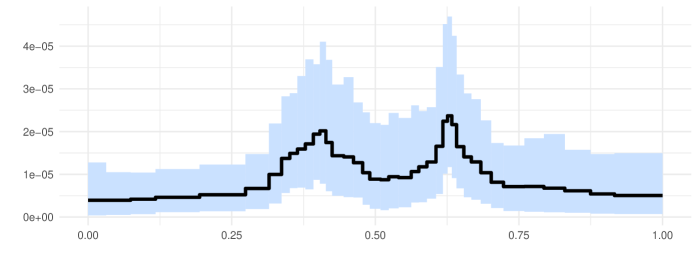
Figure 3. Top: Natural logarithm of the EUR/USD exchange rate data for 2 March 2015 analysed in Section 4. Bottom: Posterior mean (black curve) and pointwise 95% credible band (blue band) for the volatility function. The time axis is rescaled to $[0,1]$.

Financial time series often contain jumps, accurate detection of which is a delicate task. As this section serves illustrative purposes only, for simplicity we ignore jumps in our analysis. For high frequency data, volatility estimates are expected to recover quickly after infrequent jumps in the underlying process. This should in particular be the case for our learning procedure, given that we model the volatility as a piecewise constant function, which can be viewed as an estimate of the “histogramised” true volatility. Indeed, effects of infrequent jumps in the underlying process are likely to get smoothed out by averaging (we make no claim of robustness of our procedure with respect to possible presence of large jumps in the process $X$, or densely clustered small jumps). An alternative here would have been to use a heuristic jump removal technique, such as the ones discussed in Sabel et al. (2015); next one could have applied our Bayesian procedure on the resulting “cleaned” data.

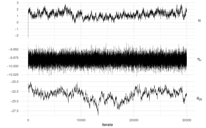
Figure 7. Log trace plots for the real data example of Section 4. Top: $\alpha$, middle: $\eta_{v}$, bottom: $\theta_{20}$.

We report inference results in Figure 3, where time is rescaled to the interval $[0,1]$, so that $t=0$ corresponds to the midnight and $t=0.5$ to noon. As seen from the plot, there is considerable uncertainty in volatility estimates. Understandably, the volatility is lower during the night hours. It also displays two peaks corresponding to the early morning and late afternoon parts of the day. Finally, we give several trace plots of the generated Markov chains in Figure 7. The algorithm took ca. 33 minutes to complete. In Figure 4 we give inference results obtained via further subsampling of the data, retaining $50\%$ of the observations. The posterior mean is quite similar to that in Figure 3, whereas the wider credible band reflects greater inferential uncertainty due to a smaller sample size. The figure provides a partial validation of the model we use.

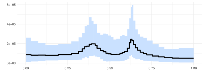
Figure 4. Posterior mean (black curve) and pointwise 95% credible band (blue band) for the volatility of the further subsampled EUR/USD exchange rate data analysed in Section 4. The time axis is rescaled to $[0,1]$.

5. Discussion

In this paper we studied a practical nonparametric Bayesian approach to volatility learning under microstructure noise. From the statistical theory point of view, the problem is much more difficult than volatility learning from noiseless observations. Hence, accurate inference on volatility under microstructure noise requires large amounts of data, which, fortunately, are available in financial applications. On the other hand, it becomes important to devise a learning method that scales well with the size of the data. This is indeed the case for the technique we study in this work. Our prior specification and a deliberate, but asymptotically harmless misspecification of the drift by taking $b\equiv 0$ are clever choices which enable to combine our earlier work in Gugushvili et al. (2018a) with FFBS algorithm for Gaussian linear state space models. This directly gives a conceptually simple algorithm (Gibbs sampler) to obtain samples from the posterior, from which measures of inferential uncertainty can be extracted in a straightforward way. Given the promising results we have obtained, we plan to further pursue the current research direction for exploring for example online Bayesian learning of the volatility. This may require the use of sequential Monte Carlo methods (see, e.g., Cappé et al. (2007)). Another very interesting topic is to explicitly account for the possible presence of jumps in financial time series within the statistical model.

Appendix A

We denote the inverse Gamma distribution with shape parameter $\alpha>0$ and scale parameter $\beta>0$ by $\operatorname{IG}(\alpha,\beta)$. Its density is

$$x\mapsto\frac{\beta^{\alpha}}{\Gamma(\alpha)}x^{-\alpha-1}e^{-\beta/x},\quad x>0.$$

By $N(\mu,\sigma^{2})$ we denote a normal distribution with mean $\mu\in\mathbb{R}$ and variance $\sigma^{2}>0$. The uniform distribution on an interval $[a,b]$ is denoted by $\operatorname{Uniform}(a,b).$ For a random variate $X$, the notation $X\sim p$ stands for the fact that $X$ is distributed according to a density $p$, or is drawn according to a density $p$. Conditioning of a random variate $X$ on a random variate $Y$ is denoted by $X\mid Y$. By $\lfloor x\rfloor$ we denote the integer part of a real number $x$. The notation $p\propto q$ for a density $p$ denotes the fact that a positive function $q$ is an unnormalised density corresponding to $p$: $p$ can be recovered from $q$ as $q/\int q$. Finally, we use the shorthand notation $a_{k:\ell}=(a_{k},\ldots,a_{\ell})$.

Appendix B

B.1. Drawing $x_{0:n}$

We first describe how to draw the state vector $x_{0:n}$ conditional on all other parameters in the model and the data $y_{1:n}$. Note that for $u_{i}$ in (5) we have by (4) that $u_{i}\sim N(0,w_{i})$, where

(9) $$\begin{split}w_{i}&=\theta_{k}\Delta_{i},\quad i\in[(k-1)m+1,km],\quad k=1,\ldots,N-1,\\ w_{i}&=\theta_{N}\Delta_{i},\quad i\in[(N-1)m+1,n].\end{split}$$

By equation (4.21) in Petris et al. (2009), write (we omit dependence on $\theta_{1:N},\eta_{v}$ in our notation, as they stay fixed in this step)

$$p(x_{0:n}|y_{1:n})=\prod_{i=0}^{n}p(x_{i}|x_{i+1:n},y_{1:n}),$$

where the factor with $i=n$ in the product on the righthand side is the filtering density $p(x_{n}|y_{1:n})$. This distribution is in fact $N(\mu_{n},C_{n})$, with the mean $\mu_{n}$ and variance $C_{n}$ obtained from Kalman recursions

$$\mu_{i}=\mu_{i-1}+K_{i}e_{i},\quad C_{i}=K_{i}\eta_{v},\quad i=1,\ldots,n.$$

Here

$$K_{i}=\frac{C_{i-1}+w_{i}}{C_{i-1}+w_{i}+\eta_{v}},\quad i=1,\ldots,n,$$

is the Kalman gain. Furthermore, $e_{i}=y_{i}-\mu_{i-1}$ is the one-step ahead prediction error. See Petris et al. (2009), Section 2.7.2. This constitutes the forward pass of the FFBS.

Next, in the backward pass, one draws backwards in time $\widetilde{x}_{n}\sim N(\mu_{n},C_{n})$ and $\widetilde{x}_{n-1},\ldots\widetilde{x}_{0}$ from the densities $p(x_{i}|\widetilde{x}_{i+1},y_{1:n})$ for $i=n-1,n-2,\ldots,0$. It holds that $p(x_{i}|\widetilde{x}_{i+1:n},y_{1:n})=p(x_{i}|\widetilde{x}_{i+1},y_{1:n})$, and the latter distribution is $N(h_{t},H_{t})$, with

$$h_{i}=\mu_{i}+\frac{C_{i}}{C_{i}+w_{i+1}}(\widetilde{x}_{i+1}-\mu_{i}),\quad H_{i}=\frac{C_{i}w_{i+1}}{C_{i}+w_{i+1}}.$$

For every $i$, these expressions depend on a previously generated $\widetilde{x}_{i+1}$ and other known quantities only. The sequence $\widetilde{x}_{0},\widetilde{x}_{1},\ldots,\widetilde{x}_{n}$ is a sample from $p(x_{0:n}|y_{1:n})$. See Section 4.4.1 in Petris et al. (2009) for details on FFBS.

B.2. Drawing $\eta_{v}$

Using the likelihood expression from Subsection 2.3 and the fact that $\eta_{v}\sim\operatorname{IG}(\alpha_{v},\beta_{v})$, one sees that the full conditional distribution of $\eta_{v}$ is given by

$$\eta_{v}|x_{1:n},y_{1:n}\sim\operatorname{IG}\left(\alpha_{v}+\frac{n}{2},\beta_{v}+\frac{1}{2}\sum_{i=1}^{n}(y_{i}-x_{i})^{2}\right).$$

B.3. Drawing $\theta_{1:N}$ and $\zeta_{2:N}$

Using the likelihood expression from Subsection 2.3 and the conditional distributions in (7), one sees that the full conditional distributions for $\theta_{1:N}$ are

$$\theta_{1}|\zeta_{2},x_{1:n} \sim\mathrm{IG}\left(\alpha_{1}+\alpha+\frac{m_{1}}{2},\,\beta_{1}+\frac{\alpha}{\zeta_{2}}+\frac{Z_{1}}{2}\right),$$

$$\theta_{k}|\zeta_{k},\zeta_{k+1},x_{1:n} \sim\mathrm{IG}\left(2\alpha+\frac{m_{k}}{2},\,\frac{\alpha}{\zeta_{k}}+\frac{\alpha}{\zeta_{k+1}}+\frac{Z_{k}}{2}\right),\quad k=2,\dots,N-1,$$

$$\theta_{N}|\zeta_{N},x_{1:n} \sim\mathrm{IG}\left(\alpha+\frac{m_{N}}{2},\,\frac{\alpha}{\zeta_{N}}+\frac{Z_{N}}{2}\right).$$

The full conditional distributions for $\zeta_{2:N}$ are

$$\zeta_{k}|\theta_{k},\theta_{k-1}\sim\operatorname{IG}\left(2\alpha,\frac{\alpha}{\theta_{k-1}}+\frac{\alpha}{\theta_{k}}\right),\quad k=2,\ldots,N.$$

B.4. Drawing $\alpha$

The unnormalised full conditional density of $\alpha$ is

$$q(\alpha)=\pi(\alpha)\left(\frac{\alpha^{\alpha}}{\Gamma(\alpha)}\right)^{2(N-1)}\exp\left(-\alpha\sum_{k=2}^{N}\frac{1}{\zeta_{k}}\left(\frac{1}{\theta_{k-1}}+\frac{1}{\theta_{k}}\right)\right)\prod_{k=2}^{N}\left(\theta_{k-1}\theta_{k}\zeta_{k}^{2}\right)^{-\alpha}.$$

The corresponding normalised density is nonstandard, and the Metropolis-within-Gibbs step (see, e.g., Tierney (1994)) is used to update $\alpha$. The specific details are exactly the same as in Gugushvili et al. (2018a).

Appendix C

Settings for the Gibbs sampler we used in Section 3 are as follows: we used a vague specification $\alpha_{1},\beta_{1}\rightarrow 0$, and also assumed that $\log\alpha\sim N(1,0.25)$ and $\eta_{v}\sim\operatorname{IG}(0.3,0.3)$ (for the Heston model we used the specification $\eta_{v}\sim\operatorname{IG}(0.001,0.001)$). Furthermore, we set $x_{0}\sim N(0,25)$. The Metropolis-within-Gibbs step to update the hyperparameter $\alpha$ was performed via an independent Gaussian random walk proposal (with a correction as in Wilkinson (2012)) with scaling to ensure the acceptance rate of ca. $30-50\%$. The Gibbs sampler was run for $30\,000$ iterations, with the first third of the samples dropped as burn-in.

Appendix D

This appendix gives several trace plots for data examples we analysed in the main body of the paper.

References

- Bezanson et al. [2017] J. Bezanson, A. Edelman, S. Karpinski, and V. B. Shah. Julia: a fresh approach to numerical computing. SIAM Rev., 59(1):65–98, 2017. ISSN 0036-1445.
- Cappé et al. [2007] O. Cappé, S. J. Godsill, and E. Moulines. An overview of existing methods and recent advances in sequential Monte Carlo. Proceedings of the IEEE, 95(5):899–924, may 2007. ISSN 0018-9219.
- Cemgil and Dikmen [2007] A. T. Cemgil and O. Dikmen. Conjugate gamma Markov random fields for modelling nonstationary sources. In Mike E. Davies, Christopher J. James, Samer A. Abdallah, and Mark D. Plumbley, editors, Independent Component Analysis and Signal Separation: 7th International Conference, ICA 2007, London, UK, September 9–12, 2007. Proceedings, pages 697–705. Springer Berlin Heidelberg, Berlin, Heidelberg, 2007. ISBN 978-3-540-74494-8.
- Cox et al. [1985] John C. Cox, Jonathan E. Ingersoll, and Stephen A. Ross. A theory of the term structure of interest rates. Econometrica, 53(2):385–407, 1985.
- Fan and Gijbels [1995] Jianqing Fan and Irène Gijbels. Data-driven bandwidth selection in local polynomial fitting: variable bandwidth and spatial adaptation. J. Roy. Statist. Soc. Ser. B, 57(2):371–394, 1995. ISSN 0035-9246.
- Ghosal and van der Vaart [2017] S. Ghosal and A. van der Vaart. Fundamentals of nonparametric Bayesian inference, volume 44 of Cambridge Series in Statistical and Probabilistic Mathematics. Cambridge University Press, Cambridge, 2017. ISBN 978-0-521-87826-5.
- Gugushvili et al. [2017] S. Gugushvili, F. van der Meulen, M. Schauer, and P. Spreij. Nonparametric Bayesian estimation of a Hölder continuous diffusion coefficient. ArXiv e-prints, 2017.
- Gugushvili et al. [2018a] S. Gugushvili, F. van der Meulen, M. Schauer, and P. Spreij. Nonparametric Bayesian volatility estimation. ArXiv e-prints, 2018a.
- Gugushvili et al. [2018b] S. Gugushvili, F. van der Meulen, M. Schauer, and P. Spreij. Fast and scalable non-parametric Bayesian inference for Poisson point processes. ArXiv e-prints, 2018b.
- Heston [1993] Steven L. Heston. A closed-form solution for options with stochastic volatility with applications to bond and currency options. Rev. Financial Stud., 6(2):327–343, 1993.
- Hoffmann et al. [2012] M. Hoffmann, A. Munk, and J. Schmidt-Hieber. Adaptive wavelet estimation of the diffusion coefficient under additive error measurements. Ann. Inst. Henri Poincaré Probab. Stat., 48(4):1186–1216, 2012. ISSN 0246-0203.
- Ignatieva and Platen [2012] K. Ignatieva and E. Platen. Estimating the diffusion coefficient function for a diversified world stock index. Comput. Statist. Data Anal., 56(6):1333–1349, 2012. ISSN 0167-9473.
- Jacod et al. [2009] J. Jacod, Y. Li, P.A. Mykland, M. Podolskij, and M. Vetter. Microstructure noise in the continuous case: the pre-averaging approach. Stochastic Process. Appl., 119(7):2249–2276, 2009. ISSN 0304-4149.
- Müller and Mitra [2013] P. Müller and R. Mitra. Bayesian nonparametric inference—why and how. Bayesian Anal., 8(2):269–302, 2013. ISSN 1936-0975.
- Müller et al. [2015] P. Müller, F. A. Quintana, A. Jara, and T. Hanson. Bayesian nonparametric data analysis. Springer Series in Statistics. Springer, Cham, 2015. ISBN 978-3-319-18967-3; 978-3-319-18968-0.
- Munk and Schmidt-Hieber [2010] A. Munk and J. Schmidt-Hieber. Lower bounds for volatility estimation in microstructure noise models. In Borrowing strength: theory powering applications—a Festschrift for Lawrence D. Brown, volume 6 of Inst. Math. Stat. (IMS) Collect., pages 43–55. Inst. Math. Statist., Beachwood, OH, 2010.
- Musiela and Rutkowski [2005] M. Musiela and M. Rutkowski. Martingale methods in financial modelling, volume 36 of Stochastic Modelling and Applied Probability. Springer-Verlag, Berlin, 2 edition, 2005. ISBN 3-540-20966-2.
- Mykland and Zhang [2009] P. A. Mykland and L. Zhang. Inference for continuous semimartingales observed at high frequency. Econometrica, 77(5):1403–1445, 2009. ISSN 0012-9682.
- Mykland and Zhang [2012] P. A. Mykland and L. Zhang. The econometrics of high-frequency data. In Statistical methods for stochastic differential equations, volume 124 of Monogr. Statist. Appl. Probab., pages 109–190. CRC Press, Boca Raton, FL, 2012.
- Papaspiliopoulos et al. [2013] Omiros Papaspiliopoulos, Gareth O. Roberts, and Osnat Stramer. Data augmentation for diffusions. J. Comput. Graph. Statist., 22(3):665–688, 2013. ISSN 1061-8600.
- Petris et al. [2009] G. Petris, S. Petrone, and P. Campagnoli. Dynamic linear models with R. Use R! Springer, New York, 2009. ISBN 978-0-387-77237-0.
- Reiß [2011] M. Reiß. Asymptotic equivalence for inference on the volatility from noisy observations. Ann. Statist., 39(2):772–802, 2011. ISSN 0090-5364.
- Sabel et al. [2015] T. Sabel, J. Schmidt-Hieber, and A. Munk. Spot volatility estimation for high-frequency data: adaptive estimation in practice. In Modeling and stochastic learning for forecasting in high dimensions, volume 217 of Lect. Notes Stat., pages 213–241. Springer, Cham, 2015.
- Schauer and Gugushvili [2018] Moritz Schauer and Shota Gugushvili. MicrostructureNoise, may 2018. URL https://doi.org/10.5281/zenodo.1241024.
- Silverman [1986] B. W. Silverman. Density estimation for statistics and data analysis. Monographs on Statistics and Applied Probability. Chapman & Hall, London, 1986. ISBN 0-412-24620-1.
- Tanner and Wong [1987] M. A. Tanner and W. H. Wong. The calculation of posterior distributions by data augmentation. J. Amer. Statist. Assoc., 82(398):528–550, 1987. ISSN 0162-1459. With discussion and with a reply by the authors.
- Tierney [1994] L. Tierney. Markov chains for exploring posterior distributions. Ann. Statist., 22(4):1701–1762, 1994. ISSN 0090-5364. With discussion and a rejoinder by the author.
- van der Meulen and Schauer [2017] F. van der Meulen and M. Schauer. Bayesian estimation of discretely observed multi-dimensional diffusion processes using guided proposals. Electron. J. Stat., 11(1):2358–2396, 2017. ISSN 1935-7524.
- van der Ploeg [2006] A. P. C. van der Ploeg. Stochastic volatility and the pricing of financial derivatives. PhD thesis, University of Amsterdam, 2006.
- Wilkinson [2012] D. J. Wilkinson. Metropolis Hastings MCMC when the proposal and target have differing support, 2012. URL https://darrenjw.wordpress.com/2012/06/04/metropolis-hastings-mcmc-when-the-proposal-and-target-have-differing-support/. Online; accessed on 23 December 2017.