Influence of diffuse surface scattering on the stability of superconducting phases with spontaneous surface current generated by Andreev bound states

Abstract

We report a theoretical study on the phase transition between superconducting states with and without spontaneous surface current. The phase transition takes place due to the formation of surface Andreev bound states in unconventional superconductors. Based on the quasiclassical theory of superconductivity, we examine the influence of atomic-scale surface roughness on the surface phase transition temperature $T_{s}$. To describe the surface effect, the boundary condition for the quasiclassical Green’s function is parameterized in terms of specularity (the specular reflection probability in the normal state at the Fermi level). This boundary condition allows systematic study of the surface effect ranging from the specular limit to the diffuse limit. We show that diffuse quasiparticle scattering at a rough surface causes substantial reduction of $T_{s}$ in the $d$-wave pairing state of high-$T_{c}$ cuprate superconductors. We also consider a $p$-wave pairing state in which Andreev bound states similar to those in the $d$-wave state are generated. In contrast to the $d$-wave case, $T_{s}$ in the $p$-wave state is insensitive to the specularity. This is because the Andreev bound states in the $p$-wave superconductor are robust against diffuse scattering, as implied from symmetry consideration for odd-frequency Cooper pairs induced at the surface; the $p$-wave state has odd-frequency pairs with $s$-wave symmetry, while the $d$-wave state does not.

I Introduction

Theoretical studies of the $d$-wave pairing state in high-$T_{c}$ cuprate superconductors have predicted a surface state that carries a spontaneous surface current and locally breaks time-reversal symmetry $\mathcal{T}$. The authors of Ref. MatsumotoShiba, demonstrated that a pairing state with $\mathcal{T}$-breaking symmetry such as $d+is$ is stabilized near the surface by a subdominant pairing interaction and this surface state with broken $\mathcal{T}$ generates a spontaneous current. The spontaneous surface current was later shown to occur also in the absence of subdominant interactions SeijiJPSJ1997 . The origin of the local symmetry breaking lies in the existence of Andreev bound states (ABSs) that form, in the presence of $\mathcal{T}$, a flat band at zero energy (Fermi level) Hu ; TanakaKashiwaya ; KashiwayaTanaka . Those midgap ABSs drive the instability of the $\mathcal{T}$-preserving $d$-wave phase toward a $\mathcal{T}$-breaking phase. In the latter superconducting (SC) phase, the bound-state band is shifted from the Fermi level and thereby the surface free energy can be lowered SigristPTP . The self-induced vector potential associated with the spontaneous current provides a mechanism for the energy shift SeijiJPSJ1997 ; Lofwander . The subdominant order parameter itself also brings about the energy shift MatsumotoShiba ; Fogelstrom . In restricted geometries such as thin films VorontsovPRL ; SeijiJPSJ2015 ; MiyawakiPRB2015 ; MiyawakiJLTP2017 , a direct phase transition from the normal state to the $\mathcal{T}$-breaking state was shown to be possible when the confinement size is of the order of the coherent length $\xi_{0}$. Recently, spontaneous generation of a vortex chain structure was predicted to occur along the surface of the cuprate superconductors Hakansson ; Holmvall ; HolmvallPHD .

In this paper, we are concerned with the surface phase transition between the SC states with and without the spontaneous surface current. In general, the surface physics sensitively depends on the nature of the boundary condition. For example, surface roughness causes significant modification of the surface density of states (SDOS) in superconductors and superfluids Zhang ; Yamada ; Yamamoto ; VorontsovSauls ; NagaiJPSJ ; MurakawaPRL ; MurakawaJPSJ ; Okuda . In the case of the $d$-wave SC state, diffuse quasiparticle scattering by the surface roughness results in substantial broadening of SDOS at zero energy Yamada . The broadening of zero-energy SDOS suggests the reduction of the surface phase transition temperature $T_{s}$ Barash . Here, we address the rough surface problem with the purpose of evaluating the robustness of the $\mathcal{T}$-breaking SC phase against diffuse surface scattering. We parameterize the boundary problem in terms of the specularity of the surface NagaiJPSJ ; MurakawaPRL ; MurakawaJPSJ ; Okuda . This parameterization allows us to treat the surface effect ranging from the specular limit to the diffuse limit in a unified way (Fig. 1). For simplicity, we do not take into consideration impurity effects Barash , subdominant pairing channels MatsumotoShiba ; Fogelstrom , and the possibility of the surface vortex chain state Hakansson ; Holmvall ; HolmvallPHD .

We consider not only the $d$-wave state but also a $p$-wave (polar) state (Fig. 2). The two SC states have a common symmetry such that the gap function felt by quasiparticles changes sign for specular reflection processes. Because of this symmetry, the midgap ABSs appear in both superconductors Hu ; HaraNagai ; OhashiTakada . When the surface is specular, the midgap ABSs manifest in SDOS as a zero-energy peak. As mentioned above, this peak in the $d$-wave state is broadened in the presence of surface roughness. On the other hand, SDOS in the $p$-wave polar state is hardly affected by diffuse scattering Yamamoto . We show that $T_{s}$ in the $p$-wave state is insensitive to surface roughness, while in the $d$-wave state the broadening of zero-energy SDOS gives rise to a substantial reduction of $T_{s}$. The difference between the two SC states in the sensitivity to surface roughness can qualitatively be understood from symmetry consideration for odd-frequency Cooper pairs induced at the surface of the two SC states. This point will be discussed in the final part of Sec. III.

Our calculations are based on the quasiclassical theory of superconductivity Eilenberger ; LarkinOvchinnikov . We outline the theoretical formulation in Sec. II. The rough surface effect is described by random $S$-matrix theory NagatoJLTP , from which one can obtain the specularity-dependent boundary condition for the quasiclassical equation. We numerically solve Maxwell’s equations along with the quasiclassical equation to determine the vector potential spontaneously induced in the $\mathcal{T}$-breaking SC phase. The surface value of the vector potential, which is proportional to the total spontaneous magnetic field, exhibits a temperature dependence typical for a second-order phase transition. We determine the transition temperature $T_{s}$ for various values of specularity by calculating the linear response of the system to the vector potential. Those numerical results are presented in Sec. III. Our conclusions are summarized in Sec. IV.

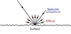
Figure 1: Scattering at a rough surface parameterized by specularity (specular reflection probability) $R$. An incident quasiparticle in the normal state at the Fermi level is scattered specularly with probability $R$ and diffusively with probability $1-R$ [see Eq. (45)]. The specular and diffuse limits correspond to $R=1$ and $R=0$, respectively.

II Quasiclassical theory

The quasiclassical theory is formulated in terms of a Green’s function $\hat{g}(\bm{r},\hat{p},\epsilon)$, which is a $4\times 4$ matrix in Nambu space. Here, $\bm{r}$ is the real-space position vector, $\hat{p}$ a unit vector to specify the Fermi-surface position, and $\epsilon$ a complex energy variable. The four-dimensional Nambu space is spanned by spin and particle-hole degrees of freedom. From symmetry consideration, the quasiclassical Green’s function $\hat{g}$ is found to have the matrix structure (Appendix A)

$$\hat{g}(\bm{r},\hat{p},\epsilon)=\begin{bmatrix}ig(\bm{r},\hat{p},\epsilon)&f(\bm{r},\hat{p},\epsilon)\\ f(\bm{r},-\hat{p},-\epsilon^{*})^{*}&-ig(\bm{r},-\hat{p},-\epsilon^{*})^{*}\\ \end{bmatrix},$$ (1)

where the elements are $2\times 2$ matrices in spin space. The spatial evolution of $\hat{g}$ is governed by the Eilenberger equation

$$i\hbar\bm{v}_{\hat{p}}\cdot\nabla_{\bm{r}}\hat{g}=[\hat{g},\ (\epsilon-\hat{\Delta})\hat{\rho}_{3}]$$ (2)

supplemented by the normalization condition

$$\hat{g}^{2}(\bm{r},\hat{p},\epsilon)=-1$$ (3)

and appropriate boundary conditions depending on the geometry of system. The gradient term on the left-hand side of Eq. (2) connects $\hat{g}$ at different spatial points on a straight line corresponding to the classical trajectory along the Fermi velocity $\bm{v}_{\hat{p}}$. On the right-hand side,

$$\hat{\Delta}=\begin{bmatrix}0&&\Delta(\bm{r},\hat{p})\\ \Delta(\bm{r},\hat{p})^{\dagger}&&0\\ \end{bmatrix}$$ (4)

is the Nambu-space gap matrix and $\hat{\rho}_{3}$ is the third Pauli matrix in particle-hole space. In superconductors with a spontaneous surface current, a magnetic field $\bm{B}(\bm{r})=\nabla_{\bm{r}}\times\bm{A}(\bm{r})$ is induced near the surface. The current-carrying state can be treated by replacing $\epsilon$ in Eq. (2) as

$$\epsilon\to\epsilon-\hbar\bm{v}_{\hat{p}}\cdot\bm{Q}(\bm{r})/2,$$ (5)

where $\bm{Q}(\bm{r})=-(2e/c\hbar)\bm{A}(\bm{r})$ with $e$ ($e<0$) being the electron charge and $c$ the speed of light. The magnetic field $\bm{B}(\bm{r})$ is related to the current density $\bm{J}(\bm{r})$ by Maxwell’s equation

$$\nabla_{\bm{r}}\times\bm{B}(\bm{r})=\frac{4\pi}{c}\bm{J}(\bm{r}).$$ (6)

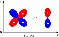
Figure 2: Semi-infinite superconductor. The surface is located at $y=0$ and a quasi-two-dimensional superconductor occupies the $y>0$ space. The superconductor is in the $d_{xy}$-wave (left) or $p_{y}$-wave (right) pairing states.

The gap matrix $\Delta(\bm{r},\hat{p})$ and the current density $\bm{J}(\bm{r})$ can be determined from $\hat{g}(\bm{r},\hat{p},\epsilon)$ on the imaginary axis of the complex $\epsilon$ plane, i.e., $\hat{g}(\bm{r},\hat{p},i\epsilon_{n})$ at the Matsubara energies $\epsilon_{n}=(2n+1)\pi/\beta$ with $n=0,\pm 1,\pm 2,\cdots$, and $\beta=1/k_{B}T$ being the inverse temperature. The corresponding equations are

$$\Delta(\bm{r},\hat{p})=N(0)\frac{\pi}{\beta}\sideset{}{{}^{\prime}}{\sum}_{\epsilon_{n}}\left\langle V_{\hat{p}\hat{p}^{\prime}}f(\bm{r},\hat{p}^{\prime},i\epsilon_{n})\right\rangle_{\hat{p}^{\prime}},$$ (7)

$$\bm{J}(\bm{r})=eN(0)\frac{\pi}{\beta}\sum_{\epsilon_{n}}{\rm Im}\left\langle\bm{v}_{\hat{p}}\,{\rm Tr}\,g(\bm{r},\hat{p},i\epsilon_{n})\right\rangle_{\hat{p}},$$ (8)

where $N(0)$ is the density of states (per spin) in the normal state at the Fermi level and $V_{\hat{p}\hat{p}^{\prime}}$ the pairing interaction. The notation

$$\langle\cdots\rangle_{\hat{p}}\equiv\frac{\int(\cdots){d^{2}p_{F}}/{|\bm{v}_{\hat{p}}|}}{\int{d^{2}p_{F}}/{|\bm{v}_{\hat{p}}|}}$$ (9)

denotes the average over the Fermi surface. The prime on the sum in Eq. (7) means that a cutoff is necessary for the Matsubara sum.

From $\hat{g}$, one can also get information on the quasiparticle density of states. The angle-resolved local density of states, normalized to be unity at an energy $E$ sufficiently larger than the SC gap, is given in terms of the diagonal elements of $\hat{g}$ with $\epsilon$ on the real axis:

$$n(\bm{r},\hat{p},E)={\rm Re}\left[\frac{1}{2}{\rm Tr}\,g(\bm{r},\hat{p},E+i\delta)\right],$$ (10)

where $\delta$ is an infinitesimal positive constant defining the retarded Green’s function.

In the actual calculation of the quasiclassical Green’s function, we used the Riccati parameterization method EschrigPRB . In this method, the spin-space matrix Green’s functions $g$ and $f$ are expressed as (Appendix A)

$$g(\bm{r},\hat{p},\epsilon) =\frac{2}{1-\mathcal{D}(\bm{r},\hat{p},\epsilon)\mathcal{D}(\bm{r},-\hat{p},-\epsilon^{*})^{*}}-1,$$ (11)

$$f(\bm{r},\hat{p},\epsilon) =[g(\bm{r},\hat{p},\epsilon)+1]\mathcal{D}(\bm{r},\hat{p},\epsilon),$$ (12)

with $\mathcal{D}(\bm{r},\hat{p},\epsilon)$ obeying the Riccati-type differential equation

$$\hbar\bm{v}_{\hat{p}}\cdot\nabla_{\bm{r}}\mathcal{D}=2i\epsilon\mathcal{D}+\Delta(\bm{r},\hat{p})-\mathcal{D}\Delta(\bm{r},\hat{p})^{\dagger}\mathcal{D}.$$ (13)

We note again that $\epsilon$ in Eq. (13) is replaced by Eq. (5) when surface current flows.

We apply the quasiclassical theory to a semi-infinite geometry as depicted in Fig. 2. A quasi-two-dimensional superconductor with a flat surface at $y=0$ occupies the $y>0$ space. The quasi-two-dimensionality is described by a cylindrical Fermi surface with an isotropic Fermi velocity $|\bm{v}_{\hat{p}}|=v_{F}$. The surface may have atomic-scale irregularity, though it is assumed to be macroscopically flat. We consider the effect of the surface roughness by parameterizing the boundary condition for Eq. (13) in terms of the specularity $R$ defined as the specular reflection probability in the normal state at the Fermi level (Fig. 1). The boundary condition is obtained from the random-$S$ matrix theory developed in Ref. NagatoJLTP, . The outline of this theory and the explicit expression for the boundary condition are given in Appendix B. We characterize the SC phase with broken $\mathcal{T}$ by the vector fields

$$\bm{Q}(\bm{r})=Q_{x}(y)\bm{e}_{x},\ \bm{B}(\bm{r})=B_{z}(y)\bm{e}_{z},\ \bm{J}(\bm{r})=J_{x}(y)\bm{e}_{x},$$

where $\bm{e}_{i}$ is the unit vectors along the $i$-axis of real-space coordinate.

The above SC system is assumed to be in $d_{xy}$-wave or $p_{y}$-wave states with the gap matrix

$$\Delta(\bm{r},\hat{p})=\Delta_{0}(y)\zeta(\hat{p})s_{\sigma}.$$ (14)

For the $d_{xy}$-wave state, $\zeta(\hat{p})=2\sqrt{2}\,\hat{p}_{x}\hat{p}_{y}$ and $s_{\sigma}=i\sigma_{2}$. For the $p_{y}$-wave state, $\zeta(\hat{p})=\sqrt{2}\,\hat{p}_{y}$ and $s_{\sigma}=\bm{s}\cdot\bm{\sigma}i\sigma_{2}$. Here, $\bm{\sigma}=(\sigma_{1},\sigma_{2},\sigma_{3})$ is the Pauli matrix and $\bm{s}$ is a unit vector in spin space. Because our model system has rotational symmetry in spin space, the direction of $\bm{s}$ may be chosen arbitrarily. The basis function $\zeta(\hat{p})$ is normalized as $\langle\zeta^{2}(\hat{p})\rangle_{\hat{p}}=1$. The single-component SC states can be characterized by the pairing interaction of the form $V_{\hat{p}\hat{p}^{\prime}}=V\zeta(\hat{p})\zeta(\hat{p}^{\prime})$. The interaction parameter $V$ is related to the transition temperature $T_{c}$ between the normal and bulk-SC states by

$$\frac{1}{N(0)V}=2\pi k_{B}T_{c}\sideset{}{{}^{\prime}}{\sum}_{\epsilon_{n}>0}\frac{1}{\epsilon_{n}}\approx\ln(1.13\epsilon_{c}/k_{B}T_{c}),$$ (15)

where $\epsilon_{c}$ denotes the cutoff energy for the Matsubara sum.

III Numerical results

For numerical calculation of $Q_{x}(y)$, $B_{z}(y)$, and $J_{x}(y)$, we introduce the dimensionless quantities

$$q_{x}(y) =\xi_{0}Q_{x}(y),$$ (16)

$$b_{z}(y) =\frac{2|e|}{\hbar c}\lambda_{0}\xi_{0}B_{z}(y),$$ (17)

$$j_{x}(y) =\frac{8\pi|e|}{\hbar c^{2}}\lambda_{0}^{2}\xi_{0}J_{x}(y)=\frac{J_{x}(y)}{\pi|e|v_{F}N(0)k_{B}T_{c}},$$ (18)

where $\xi_{0}=\hbar v_{F}/2\pi k_{B}T_{c}$ is the coherence length and $\lambda_{0}=(c^{2}/4\pi e^{2}N(0)v_{F}^{2})^{1/2}$ is the London penetration depth at $T=0$. The dimensionless fields are determined from Maxwell’s equations

$$\lambda_{0}\frac{dq_{x}(y)}{dy}=-b_{z}(y),$$ (19)

$$\lambda_{0}\frac{db_{z}(y)}{dy}=j_{x}(y),$$ (20)

along with $j_{x}(y)$ obtained from Eq. (8). The boundary conditions are $q_{x}(\infty)=0$ and $b_{z}(0)=0$. In the self-consistent calculation of the fields, we neglect, for simplicity, the surface pairbreaking effect and put $\Delta_{0}(y)=\Delta_{0}(\infty)$. This approximation will not be serious because the low-energy structure of SDOS is insensitive to the self-consistency of the gap function NagatoNagaiPRB .

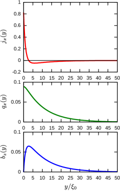
Figure 3: Spatial distribution of $j_{x}(y)$, $q_{x}(y)$, and $b_{z}(y)$ in the $d_{xy}$ superconductor with $\lambda_{0}/\xi_{0}=10.0$ at $T/T_{c}=0.02$. The surface is assumed to be specular ($R=1$).

In Fig. 3, we plot the typical spatial distribution of the fields $j_{x}(y)$, $q_{x}(y)$, and $b_{z}(y)$ induced spontaneously in the $d_{xy}$ superconductor. The results are shown for $R=1$. The current $j_{x}(y)$ takes a large positive value at the surface ($y=0$) owing to the formation of midgap ABSs. As the distance $y$ from the surface increases, $j_{x}(y)$ decreases and becomes negative at $y\sim\xi_{0}$. The negative (screening) current prevents the spontaneous magnetic field $b_{z}(y)$ from penetrating into the superconductor. The total current $\int_{0}^{\infty}dy\,j_{x}(y)$ vanishes SeijiJPSJ1997 ; OhashiMomoi ; KusamaOhashi , as assured by Maxwell’s equation (20) with the boundary condition $b_{z}(0)=0$. The fields for $R\neq 1$ exhibit similar $y$ dependence.

The spontaneous surface current appears at low temperatures after a second-order phase transition from the conventional $\mathcal{T}$-preserving SC state. To demonstrate the surface phase transition in the $d_{xy}$ superconductor, we plot in Fig. 4 the temperature dependence of $q_{x}(0)$, which is proportional to the total magnetic field induced by the spontaneous current [see Eq. (19)]. The symbols are the results obtained by numerically solving Maxwell’s equations at several temperatures. The solid lines are fits using

$$q_{x}(0)=C_{1}\tanh\left(C_{2}\sqrt{C_{3}/t-1}\right),$$ (21)

where the $C_{i}$’s are fitting parameters and $t=T/T_{c}$ is the reduced temperature. The numerical data are well fitted by Eq. (21), in which a second-order phase transition is assumed to take place at $t=C_{3}$ corresponding to the surface phase transition temperature $T_{s}$ scaled by $T_{c}$. As we increase the parameter $\lambda_{0}/\xi_{0}$, the reduced transition temperature $T_{s}/T_{c}$ decreases [Fig. 4 (a)]. The origin of this property is the different length scales between the surface current carried by ABSs and the conventional screening current. The former is localized within the surface region of width $\sim\xi_{0}$. The latter flows within a width $\sim\lambda_{0}$. To satisfy the condition of vanishing total current at a finite $q_{x}(0)$, larger ABS current and therefore lower temperature is required for larger $\lambda_{0}/\xi_{0}$. Figure 4 (b) demonstrates the effect of diffuse surface scattering on $q_{x}(0)$. The reduced transition temperature $T_{s}/T_{c}$ is suppressed by diffuse scattering and depends rather sensitively on the specularity $R$. The corresponding suppression of $b_{z}(y)$ at $T/T_{c}=0.05$ is shown in Fig. 5.

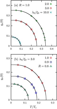
Figure 4: Temperature dependence of $q_{x}(0)$ in the $d_{xy}$ superconductor for (a) several $\lambda_{0}/\xi_{0}$ at $R=1.0$ and (b) several $R$ at $\lambda_{0}/\xi_{0}=3.0$. The symbols are the numerical results and the solid lines are fits using Eq. (21).

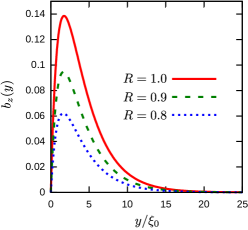
Figure 5: Spontaneous magnetic field $b_{z}(y)$ in the $d_{xy}$ superconductor with $\lambda_{0}/\xi_{0}=3.0$ at $T/T_{c}=0.05$.

To study the rough surface effect on $T_{s}/T_{c}$ in more detail, we solved the linearized Maxwell’s equations numerically

$$\int_{0}^{\infty}dy^{\prime}K(y,y^{\prime})\,q_{x}(y^{\prime})=\lambda_{0}^{2}\frac{d^{2}q_{x}(y)}{dy^{2}}.$$ (22)

The left-hand side corresponds to the linear response of $-j_{x}(y)$ to $q_{x}(y)$. The kernel $K(y,y^{\prime})$ can be obtained by expanding the quasiclassical Green’s function $g$ to linear order in $q_{x}(y)$ and substituting the linear deviation into Eq. (8). The resulting explicit formula is so lengthy that it is not shown here. We note only that $K(y,y^{\prime})$ is real and symmetric under the exchange of $y$ and $y^{\prime}$.

To solve Eq. (22), we used the finite difference formulas

$$\frac{dq_{x}}{dy}=\frac{q_{i+1}-q_{i-1}}{2h},\ \ \frac{d^{2}q_{x}}{dy^{2}}=\frac{q_{i+1}-2q_{i}+q_{i-1}}{h^{2}},$$ (23)

where $q_{i}=q_{x}(ih)$ with $i$ being an integer. Evaluating the $y^{\prime}$ integral in Eq. (22) using the trapezoidal rule, we obtain

$$\frac{K_{i0}q_{0}+K_{iN}q_{N}}{2}+\sum_{j=1}^{N-1}K_{ij}q_{j}=\mu(q_{i+1}-2q_{i}+q_{i-1}),$$

$$b_{z}(0)\propto(q_{1}-q_{-1})/2h=0,\ \ q_{N}=0,$$

where $K_{ij}=hK(ih,jh)$ and $\mu=\lambda_{0}^{2}/h^{2}$. This set of equations can be cast into the form of the generalized eigenvalue equation $\mathbb{A}\vec{q}=\mu\mathbb{B}\vec{q}$ with $\mathbb{A}$ being a real symmetric matrix and $\mathbb{B}$ being a positive-definite real symmetric matrix. Using the GNU Scientific Library, we solved it to obtain the eigenvalue $\mu$ at a given $t=T/T_{c}$ (we performed the calculations down to $t=0.01$). The resulting $\mu$-$t$ relation gives $T_{s}/T_{c}$ as a function of $\lambda_{0}/\xi_{0}$. From the numerical calculation, we found that the maximum eigenvalue $\mu_{\rm max}$ reproduces $T_{s}/T_{c}$ determined from the full (nonlinear) Maxwell’s equation (Fig. 4).

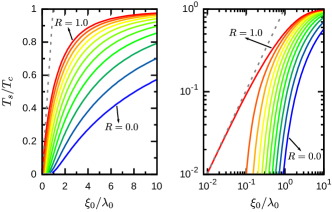
Figure 6: Reduced transition temperature $T_{s}/T_{c}$ in the $d_{xy}$ superconductor as a function of $\xi_{0}/\lambda_{0}$. The left panel is the linear plot of $T_{s}/T_{c}$ vs $\xi_{0}/\lambda_{0}$ and the right panel the corresponding log-log plot. The solid lines are, from right to left, the numerical results obtained by changing specularity $R$ from zero to unity in increments of 0.1. The dashed line corresponds to Eq. (24).

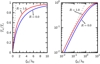
Figure 7: Reduced transition temperature $T_{s}/T_{c}$ in the $p_{y}$ superconductor as a function of $\xi_{0}/\lambda_{0}$. The left panel is the linear plot of $T_{s}/T_{c}$ vs $\xi_{0}/\lambda_{0}$ and the right panel is its log-log plot. The solid lines are the numerical results for $R=0.0$ and $1.0$. The dashed line corresponds to Eq. (24).

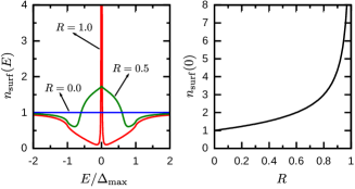
Figure 8: SDOS in the $d_{xy}$-wave SC phase without spontaneous surface current. The left panel shows the energy dependence of SDOS for $R=0.0$, $0.5$, and $1.0$. In calculating these results, we choose $\delta$ in Eq. (10) to be $10^{-3}\Delta_{\rm max}$, where $\Delta_{\rm max}=\sqrt{2}\Delta_{0}$ is the maximum value of the $\hat{p}$-dependent energy gap in the bulk SC state. In the right panel, SDOS at zero energy, Eq. (25), is plotted as a function of $R$.

In Fig. 6, we plot $T_{s}/T_{c}$ in the $d_{xy}$-wave state as a function of $\xi_{0}/\lambda_{0}$. The same plot for the $p_{y}$-wave state is shown in Fig. 7. The solid lines are the numerical results for various values of $R$. The dashed line represents the approximate formula Barash

$$\frac{T_{s}}{T_{c}}=\frac{\pi}{3}\frac{\xi_{0}}{\lambda_{0}},$$ (24)

which can be applied to strong type-II $d_{xy}$-wave and $p_{y}$-wave superconductors with $R=1.0$. When $R=1.0$, the two superconductors have almost the same $T_{s}/T_{c}$. However, the rough surface effect on $T_{s}/T_{c}$ is quite different between the two states. Diffuse surface scattering results in a substantial reduction of $T_{s}/T_{c}$ in the $d_{xy}$-wave case. On the other hand, $T_{s}/T_{c}$ in the $p_{y}$-wave state is insensitive to surface roughness. This marked difference can be understood qualitatively by observing SDOS in the absence of surface current. In Fig. 8, we plot the total SDOS, the surface value $n_{\rm surf}(E)$ of $\langle n(\bm{r},\hat{p},E)\rangle_{\hat{p}}$, in the $d_{xy}$ superconductor. In the specular limit, there is a delta-function peak at zero energy originating from midgap ABSs. This peak is broadened by diffuse scattering and the midgap SDOS, $n_{\rm surf}(0)$, decreases steeply as the specularity $R$ decreases from unity. We can show that $n_{\rm surf}(0)$ in the $d_{xy}$ superconductor depends on $R$ as Yamada

$$n_{\rm surf}(0)=\frac{1}{2}\left(\frac{1+\sqrt{R}}{\sqrt{1-\sqrt{R}}}+\frac{\sqrt{1-\sqrt{R}}}{1+\sqrt{R}}\right).$$ (25)

In the diffuse limit, $n_{\rm surf}(0)$ is suppressed to unity (then SDOS in the whole energy region coincides with that of the normal state Yamada ). The broadening of the midgap SDOS implies the reduction of the ABS current, resulting in the decrease of $T_{s}/T_{c}$ with $R$. In the $p_{y}$-wave state, SDOS also has a zero-energy peak. In contrast to the $d_{xy}$ case, however, SDOS in the $p_{y}$-wave state is quite robust against diffuse scattering Yamamoto .

The robustness of the midgap SDOS is closely related to the symmetry of odd-frequency Cooper pairing. As has been shown in the studies of boundary effects in superconductors and superfluids, ABSs appear accompanied by odd-frequency pairs (for a review, see Ref. TanakaJPSJ2012, ). Moreover, there is a relationship between the midgap density of states and the odd-frequency pair amplitude, which states the equivalence between them SeijiPRB2012 ; TsutsumiMachida ; SeijiPRB2014 ; MizushimaOddFreq . Fermi statistics requires that the odd-frequency pairs in spin-singlet and spin-triplet states have odd-parity and even-parity symmetries, respectively. The robustness of the midgap SDOS in the $p_{y}$-wave superconductor is supported by the triplet odd-frequency $s$-wave pairing induced at the surface.

IV Conclusion

We have examined numerically the influence of surface roughness on the instability temperature $T_{s}$ toward the appearance of a spontaneous surface current in unconventional superconductors. This surface phase transition is driven by midgap Andreev bound states such as formed in the $d$-wave pairing state of high-$T_{c}$ cuprate superconductors SeijiJPSJ1997 ; Lofwander ; Barash . Considering strong type-II superconductors like the cuprates and assuming the surface to be specular, one can analytically estimate $T_{s}$ and obtain the result $T_{s}\sim(\xi_{0}/\lambda_{0})T_{c}$ Lofwander ; Barash . Our numerical calculation for the specular surface reproduces this result well. In actual systems, the surface inevitably has atomic-scale surface roughness giving rise to diffuse scattering of quasiparticles. In our theory, the rough surface effect is parameterized in terms of the surface specularity (Fig. 1). We have calculated the specularity dependence of $T_{s}/T_{c}$ in the $d$-wave superconductor and found that the broadening of the midgap Andreev bound states at a rough surface causes substantial reduction of $T_{s}/T_{c}$ even for such a large specularity as $0.9$ (Fig. 6).

We have compared the result of $T_{s}/T_{c}$ for the $d$-wave state to that for the $p$-wave polar state in which the gap function has a momentum-direction dependence Hu ; HaraNagai ; OhashiTakada responsible for the generation of the midgap Andreev bound states, similar to those in the $d$-wave superconductor (Fig. 2). For the $p$-wave superconductor, we found that $T_{s}/T_{c}$ is insensitive to specularity (Fig. 7). This difference from the $d$-wave case can be accounted for by the fact that in the $p$-wave state there exist odd-frequency $s$-wave Cooper pairs behind the midgap states. The presence of the odd-frequency $s$-wave pairs assures that the midgap states are robust against diffuse surface scattering.

In the present work, we have assumed that the spontaneous surface current $\bm{J}(\bm{r})$ depends only on the coordinate perpendicular to the surface. This assumption excludes the possibility of a spontaneously-induced vortex chain structure, which has recently been predicted to appear along the surface of the high-$T_{c}$ cuprates Hakansson ; Holmvall ; HolmvallPHD . The surface phase transition temperature to the vortex chain state was reported to be higher than that for the surface state considered here. It should be noted, however, that the theoretical analysis is based on the specular surface model. The rough surface effect on the stability of this novel surface state is an important issue that remains to be examined.

Appendix A Symmetry and Nambu-space matrix structure of the quasiclassical Green’s function

The quasiclassical Green’s function $\hat{g}(\bm{r},\hat{p},\epsilon)$ defined as a $4\times 4$ Nambu-space matrix has the symmetry SereneRainer

$$\hat{g}(\bm{r},\hat{p},\epsilon) =\hat{\rho}_{1}\widetilde{\hat{g}}(\bm{r},\hat{p},\epsilon)\hat{\rho}_{1}$$ (26)

$$=\hat{\rho}_{3}\hat{g}(\bm{r},\hat{p},\epsilon^{*})^{\dagger}\hat{\rho}_{3},$$ (27)

where $\hat{\rho}_{i}$’s are the Pauli matrices in particle-hole space and the tilde transform in Eq. (26) is defined as

$$\widetilde{X}(\bm{r},\hat{p},\epsilon)=X(\bm{r},-\hat{p},-\epsilon^{*})^{*}.$$ (28)

It follows from Eq. (26) that $\hat{g}$ has the matrix structure

$$\hat{g}(\bm{r},\hat{p},\epsilon)=\begin{bmatrix}ig(\bm{r},\hat{p},\epsilon)&f(\bm{r},\hat{p},\epsilon)\\ \widetilde{f}(\bm{r},\hat{p},\epsilon)&-i\widetilde{g}(\bm{r},\hat{p},\epsilon)\\ \end{bmatrix}.$$ (29)

From Eq. (27), the spin-space matrices $g$ and $f$ are found to have the symmetry

$$g(\bm{r},\hat{p},\epsilon)=-g(\bm{r},\hat{p},\epsilon^{*})^{\dagger},$$ (30)

$$f(\bm{r},\hat{p},\epsilon)=-\widetilde{f}(\bm{r},\hat{p},\epsilon^{*})^{\dagger}=-f(\bm{r},-\hat{p},-\epsilon)^{T},$$ (31)

where the superscript $T$ denotes matrix transpose.

Introducing a spin-space matrix $\mathcal{D}(\bm{r},\hat{p},\epsilon)$ called the coherence function EschrigPRB , one can parameterize $\hat{g}(\bm{r},\hat{p},\epsilon)$ in a form that automatically satisfies the normalization condition $\hat{g}^{2}(\bm{r},\hat{p},\epsilon)=-1$:

$$\hat{g}+i=2i\begin{bmatrix}1\\ -i\widetilde{\mathcal{D}}\end{bmatrix}\frac{1}{1-\mathcal{D}\widetilde{\mathcal{D}}}\begin{bmatrix}1&-i\mathcal{D}\end{bmatrix},$$ (32)

or, equivalently,

$$\hat{g}-i=-2i\begin{bmatrix}i\mathcal{D}\\ 1\end{bmatrix}\frac{1}{1-\widetilde{\mathcal{D}}\mathcal{D}}\begin{bmatrix}i\widetilde{\mathcal{D}}&1\end{bmatrix}.$$ (33)

The symmetry relation $\eqref{eq:symrel-g-2}$ implies that the coherence function has the symmetry

$$\mathcal{D}(\bm{r},\hat{p},\epsilon^{*})^{\dagger}=\mathcal{D}(\bm{r},\hat{p},\epsilon)^{-1}.$$ (34)

Under this parameterization method, the spatial evolution of $\hat{g}(\bm{r},\hat{p},\epsilon)$ is described by the Riccati-type differential equation (13) for $\mathcal{D}(\bm{r},\hat{p},\epsilon)$, instead of the transport-like equation (2) supplemented by the normalization condition.

Appendix B Random $S$-matrix theory

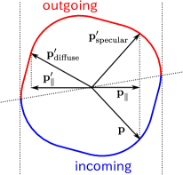
Figure 9: Fermi momenta of the incoming ($\bm{p}$) and outgoing ($\bm{p}^{\prime}$) states. The incoming (outgoing) state has a Fermi velocity towards (away from) the surface. The Fermi velocity is directed outward normal to the Fermi surface.

In the random $S$-matrix (RSM) theory NagatoJLTP , the surface effect is incorporated into the quasiclassical theory by introducing an $S$-matrix $S_{\bm{p}_{\|}^{\prime}\bm{p}_{\|}}$ in the normal state at the Fermi level and parameterizing it as

$$S_{\bm{p}_{\|}^{\prime}\bm{p}_{\|}}=-\left(\frac{1-i\eta}{1+i\eta}\right)_{\bm{p}_{\|}^{\prime}\bm{p}_{\|}}.$$ (35)

Here, $\bm{p}$ and $\bm{p}^{\prime}$ are the Fermi momenta of incoming and outgoing states, respectively, and the subscript $\|$ denotes the vector component parallel to the surface (Fig. 9). The momentum-space matrix $\eta$ is required to be an Hermite matrix so that the unitarity of $S$ is assured. When $\eta=0$, Eq. (35) is reduced to $S_{\bm{p}_{\|}^{\prime}\bm{p}_{\|}}=-\delta_{\bm{p}_{\|}^{\prime}\bm{p}_{\|}}$. This form of the $S$-matrix corresponds to the specular surface case, where $\bm{p}_{\|}$ is conserved during surface scattering processes. The diffuse scattering effect is therefore described by $\eta$. In the RSM theory, every element of $\eta$ is treated as a random variable to describe the statistical property of the surface and the statistical average of $\hat{g}$ is evaluated by employing the self-consistent Born approximation. A consequence of this procedure is that the diffuse scattering effect is characterized by the average $\overline{|\eta_{\bm{p}_{\|}^{\prime}\bm{p}_{\|}}|^{2}}\equiv\eta^{(2)}(\bm{p}_{\|}-\bm{p}_{\|}^{\prime})$.

Under this model for the $S$-matrix, the boundary condition for the averaged Green’s function is obtained as

$$\hat{g}_{\rm out}(\bm{p}_{\|},\epsilon)=\frac{1+i\hat{\gamma}_{\bm{p}_{\|}}(\epsilon)}{1-i\hat{\gamma}_{\bm{p}_{\|}}(\epsilon)}\hat{g}_{\rm in}(\bm{p}_{\|},\epsilon)\frac{1-i\hat{\gamma}_{\bm{p}_{\|}}(\epsilon)}{1+i\hat{\gamma}_{\bm{p}_{\|}}(\epsilon)},$$ (36)

where

$$\hat{\gamma}_{\bm{p}_{\|}}(\epsilon) =\sum_{\bm{p}_{\|}^{\prime}}\eta^{(2)}(\bm{p}_{\|}-\bm{p}_{\|}^{\prime})\hat{G}_{\bm{p}_{\|}^{\prime}}(\epsilon),$$ (37)

$$\hat{G}_{\bm{p}_{\|}}(\epsilon) =\frac{1}{1-i\hat{\gamma}_{\bm{p}_{\|}}(\epsilon)}\left[\hat{g}_{\rm in}(\bm{p}_{\|},\epsilon)-\hat{\gamma}_{\bm{p}_{\|}}(\epsilon)\right]\frac{1}{1+i\hat{\gamma}_{\bm{p}_{\|}}(\epsilon)}$$

$$=\frac{1}{1+i\hat{\gamma}_{\bm{p}_{\|}}(\epsilon)}\left[\hat{g}_{\rm out}(\bm{p}_{\|},\epsilon)-\hat{\gamma}_{\bm{p}_{\|}}(\epsilon)\right]\frac{1}{1-i\hat{\gamma}_{\bm{p}_{\|}}(\epsilon)}.$$

In Eq. (36), $\hat{g}_{{\rm in}({\rm out})}(\bm{p}_{\|},\epsilon)$ stands for the surface value of $\hat{g}(\bm{r},\hat{p},\epsilon)$ at the incoming (outgoing) Fermi momentum with a given parallel component $\bm{p}_{\|}$. Equation (36) with $\hat{\gamma}_{\bm{p}_{\|}}(\epsilon)=0$ ($\eta^{(2)}=0)$ gives the specular surface boundary condition

$$\hat{g}_{\rm out}(\bm{p}_{\|},\epsilon)=\hat{g}_{\rm in}(\bm{p}_{\|},\epsilon),$$ (38)

which means that the quasiclassical propagator is continuous on the trajectory along a specular reflection process. This property is lost at a rough surface because of a finite $\hat{\gamma}_{\bm{p}_{\|}}(\epsilon)$. The Nambu-space matrix $\hat{\gamma}_{\bm{p}_{\|}}(\epsilon)$ has symmetries similar to Eqs. (26) and (27) for the quasiclassical Green’s function, i.e.,

$$\hat{\gamma}_{\bm{p}_{\|}}(\epsilon) =\hat{\rho}_{1}\widetilde{\hat{\gamma}}_{\bm{p}_{\|}}(\epsilon)\hat{\rho}_{1}$$ (39)

$$=\hat{\rho}_{3}\hat{\gamma}_{\bm{p}_{\|}}(\epsilon^{*})^{\dagger}\hat{\rho}_{3}.$$ (40)

Equation (36) can be rewritten in the form

$$\hat{g}_{\rm out}(\bm{p}_{\|},\epsilon)-\hat{g}_{\rm in}(\bm{p}_{\|},\epsilon)$$

$$=2i\sum_{\bm{p}_{\|}^{\prime}}\eta^{(2)}(\bm{p}_{\|}-\bm{p}_{\|}^{\prime})[\hat{G}_{\bm{p}_{\|}^{\prime}}(\epsilon),\ \hat{G}_{\bm{p}_{\|}}(\epsilon)].$$ (41)

From this, we readily find

$$0 =\sum_{\bm{p}_{\|}}\left[\hat{g}_{\rm out}(\bm{p}_{\|},\epsilon)-\hat{g}_{\rm in}(\bm{p}_{\|},\epsilon)\right]$$ (42)

$$\propto\int_{\rm out}\frac{d^{2}p_{F}}{|\bm{v}_{\hat{p}}|}\,|v_{\hat{p}}^{\perp}|\hat{g}_{\rm out}(\bm{p}_{\|},\epsilon)-\int_{\rm in}\frac{d^{2}p_{F}}{|\bm{v}_{\hat{p}}|}\,|v_{\hat{p}}^{\perp}|\hat{g}_{\rm in}(\bm{p}_{\|},\epsilon),$$

where $v_{\hat{p}}^{\perp}$ is the Fermi velocity component perpendicular to the surface. Equation (42) guarantees that there is no net current across the surface.

The boundary condition for the coherence function is given as

$$\begin{bmatrix}i\mathcal{D}_{\rm out}(\bm{p}_{\|},\epsilon)\\ 1\end{bmatrix}C_{2\times 2}=\frac{1+i\hat{\gamma}_{\bm{p}_{\|}}(\epsilon)}{1-i\hat{\gamma}_{\bm{p}_{\|}}(\epsilon)}\begin{bmatrix}i\mathcal{D}_{\rm in}(\bm{p}_{\|},\epsilon)\\ 1\end{bmatrix},$$ (43)

where $C_{2\times 2}$ is an arbitrary spin-space matrix. The equivalence between the boundary conditions (36) and (43) can be confirmed in the following way. Using the symmetry relations (34), (39), and (40), one can convert Eq. (43) into the form

$$C_{2\times 2}^{\prime}\begin{bmatrix}i\widetilde{\mathcal{D}}_{\rm in}(\bm{p}_{\|},\epsilon)&1\end{bmatrix}=\begin{bmatrix}i\widetilde{\mathcal{D}}_{\rm out}(\bm{p}_{\|},\epsilon)&1\end{bmatrix}\frac{1+i\hat{\gamma}_{\bm{p}_{\|}}(\epsilon)}{1-i\hat{\gamma}_{\bm{p}_{\|}}(\epsilon)},$$

where $C_{2\times 2}^{\prime}$ is again an arbitrary spin-space matrix. Substituting the above two relations for the coherence function into Eq. (33), we obtain Eq. (36).

In the RSM theory, the nature of the boundary condition is specified by $\eta^{(2)}(\bm{p}_{\|}-\bm{p}_{\|}^{\prime})$. We can describe the surface effect from the specular to the diffusive limit (Fig. 1) in a unified way by expressing it as

$$\eta^{(2)}=\frac{2W}{\sum_{\bm{p}_{\|}}1},\ \ W=\frac{1-\sqrt{R}}{\left(1+\sqrt{R}\right)^{2}},$$ (44)

where $R$ is a momentum-independent parameter. Physically, $R$ corresponds to the surface specularity, SeijiJPSJ2015 ; MurakawaPRL ; MurakawaJPSJ ; Okuda which is defined as the specular reflection probability in the normal state at the Fermi level. In fact, evaluating the statistical average of $|S_{\bm{p}_{\|}^{\prime}\bm{p}_{\|}}|^{2}$ with Eq. (44), we obtain Yamamoto

$$\overline{|S_{\bm{p}_{\|}^{\prime}\bm{p}_{\|}}|^{2}}=R\delta_{\bm{p}_{\|}^{\prime}\bm{p}_{\|}}+\frac{1-R}{\sum_{\bm{p}_{\|}}1}.$$ (45)

It is obvious that the specular surface corresponds to $R=1$. The diffuse limit, where surface scattering occurs in any possible direction with equal probability $1/\sum_{\bm{p}_{\|}}1$, is achieved for $R=0$. It follows that the above one-parameter model for $\eta^{(2)}$ provides a simple interpolation formula connecting the specular and diffuse limits.

When the boundary condition is parameterized with Eq. (44), $\hat{\gamma}_{\bm{p}_{\|}}(\epsilon)$ is independent of $\bm{p}_{\|}$ and is given by

$$\hat{\gamma}(\epsilon) =\frac{2W}{1+2W+\hat{\gamma}^{2}(\epsilon)}\,\hat{g}_{0}(\epsilon),$$ (46)

$$\hat{g}_{0}(\epsilon) =\langle\hat{g}_{\rm in}(\bm{p}_{\|},\epsilon)\rangle_{\bm{p}_{\|}}=\langle\hat{g}_{\rm out}(\bm{p}_{\|},\epsilon)\rangle_{\bm{p}_{\|}},$$ (47)

where

$$\langle\cdots\rangle_{\bm{p}_{\|}}=\sum_{\bm{p}_{\|}}(\cdots)/\sum_{\bm{p}_{\|}}1.$$ (48)

Because of the symmetries (26) and (39), $\hat{g}_{0}(\epsilon)$ and $\hat{\gamma}(\epsilon)$ have the matrix structures

$$\hat{g}_{0}(\epsilon) =\begin{bmatrix}ig_{0}(\epsilon)&f_{0}(\epsilon)\\ \widetilde{f}_{0}(\epsilon)&-i\widetilde{g}_{0}(\epsilon)\end{bmatrix},$$ (49)

$$\hat{\gamma}(\epsilon) =\begin{bmatrix}ia(\epsilon)&b(\epsilon)\\ \widetilde{b}(\epsilon)&-i\widetilde{a}(\epsilon)\end{bmatrix}.$$ (50)

Finally, we note that the RSM theory in the diffuse limit gives the same boundary condition obtained from Ovchinnikov’s rough surface model Ovchinnikov ; VorontsovSauls . To see this, let us first assume that the matrix $\hat{\gamma}(\epsilon)$ in the diffuse limit, which we denote by $\hat{\gamma}_{\rm DL}(\epsilon)$, has the property

$$\hat{\gamma}_{\rm DL}^{2}(\epsilon)=-1$$ (51)

similar to the normalization condition for the quasiclassical Green’s function. It can be shown that Eq. (51) is in fact satisfied in the normal state; the quasiclassical Green’s function in the normal state is given as $\hat{g}_{N}(\epsilon)={\rm sgn}({\rm Im}[\epsilon])i\hat{\rho}_{3}$. Then Eq. (46) has the solution

$$\hat{\gamma}(\epsilon)=\frac{1-\sqrt{R}}{1+\sqrt{R}}\,\hat{g}_{N}(\epsilon).$$ (52)

When $R=0$, $\hat{\gamma}(\epsilon)=\hat{g}_{N}(\epsilon)$ and hence Eq. (51) holds. Assuming that it also holds in SC states, we can write the boundary condition (43) in the form

$$[1-i\hat{\gamma}_{\rm DL}(\epsilon)]\begin{bmatrix}i\mathcal{D}_{\rm out}(\bm{p}_{\|},\epsilon)\\ 1\end{bmatrix}=0,$$ (53)

$$\hat{\gamma}_{\rm DL}(\epsilon)=\hat{g}_{0}(\epsilon).$$ (54)

Equation (53) tells us that $\mathcal{D}_{\rm out}(\bm{p}_{\|},\epsilon)$ in the diffuse limit is independent of $\bm{p}_{\|}$. Noting this and using Eqs. (32) and (33), we readily find that $\hat{g}_{0}(\epsilon)$ has the property $\hat{g}_{0}^{2}(\epsilon)=-1$, which justifies the assumption of Eq. (51). From Eqs. (49), (53), and (54), we obtain

$$\mathcal{D}_{\rm out}(\bm{p}_{\|},\epsilon)=\frac{1}{g_{0}(\epsilon)+1}f_{0}(\epsilon)=\frac{1}{\widetilde{f}_{0}(\epsilon)}[\widetilde{g}_{0}(\epsilon)-1].$$ (55)

The second equality holds because $\hat{g}_{0}^{2}(\epsilon)=-1$. Equation (55) coincides with the boundary condition derived by Vorontsov and Sauls VorontsovSauls using Ovchinnikov’s rough surface model.

References

- (1) M. Matsumoto and H. Shiba, J. Phys. Soc. Jpn. 64, 3384 (1995); 64, 4867 (1995).
- (2) S. Higashitani, J. Phys. Soc. Jpn. 66, 2556 (1997).
- (3) C. R. Hu, Phys. Rev. Lett. 72, 1526 (1994).
- (4) Y. Tanaka and S. Kashiwaya, Phys. Rev. Lett. 74, 3451 (1995).
- (5) S. Kashiwaya and Y. Tanaka, Rep. Prog. Phys. 63, 1641 (2000).
- (6) M. Sigrist, Prog. Theor. Phys. 99, 899 (1998).
- (7) T. Löfwander, V. S. Shumeiko, and G. Wendin, Phys. Rev. B 62, R14653 (2000).
- (8) M. Fogelström, D. Rainer, and J. A. Sauls, Phys. Rev. Lett. 79, 281 (1997).
- (9) A. B. Vorontsov, Phys. Rev. Lett. 102, 177001 (2009).
- (10) S. Higashitani and N. Miyawaki, J. Phys. Soc. Jpn. 84, 033708 (2015).
- (11) N. Miyawaki and S. Higashitani, Phys. Rev. B 91, 094511 (2015).
- (12) N. Miyawaki and S. Higashitani, J. Low Temp. Phys. 187, 545 (2017).
- (13) M. Håkansson, T. Löfwander, and M. Fogelström, Nat. Phys. 11, 755 (2015).
- (14) P. Holmvall, T. Löfwander, and M. Fogelström, J. Phys.: Conf. Ser. 969, 012037 (2018).
- (15) P. Holmvall, Ph.D. thesis, Chalmers University of Technology, 2017.
- (16) W. Zhang, Phys. Lett. A 130, 314 (1988).
- (17) K. Yamada, Y. Nagato, S. Higashitani, and K. Nagai, J. Phys. Soc. Jpn. 65, 1540 (1996).
- (18) Y. Nagato, M. Yamamoto, and K. Nagai, J. Low Temp. Phys. 110, 1135 (1998).
- (19) A. B. Vorontsov and J. A. Sauls, Phys. Rev. B 68, 064508 (2003).
- (20) K. Nagai, Y. Nagato, M. Yamamoto, and S. Higashitani, J. Phys. Soc. Jpn. 77, 111003 (2008).
- (21) S. Murakawa, Y. Tamura, Y. Wada, M. Wasai, M. Saitoh, Y. Aoki, R. Nomura, Y. Okuda, Y. Nagato, M. Yamamoto, S. Higashitani, and K. Nagai, Phys. Rev. Lett. 103, 155301 (2009).
- (22) S. Murakawa, Y. Wada, Y. Tamura, M. Wasai, M. Saitoh, Y. Aoki, R. Nomura, Y. Okuda, Y. Nagato, M. Yamamoto, S. Higashitani, and K. Nagai, J. Phys. Soc. Jpn. 80, 013602 (2011).
- (23) Y. Okuda and R. Nomura, J. Phys.: Condens. Matter 24, 343201 (2012).
- (24) Y. S. Barash, M. S. Kalenkov, and J. Kurkijärvi, Phys. Rev. B 62, 6665 (2000).
- (25) J. Hara and K. Nagai, Prog. Theor. Phys. 76, 1237 (1986).
- (26) Y. Ohashi and S. Takada, J. Phys. Soc. Jpn. 65, 246 (1996).
- (27) G. Eilenberger, Z. Phys. 214, 195 (1968).
- (28) A. I. Larkin and Y. N. Ovchinnikov, Sov. Phys. JETP 28, 1200 (1969).
- (29) Y. Nagato, S. Higashitani, K. Yamada, and K. Nagai, J. Low Temp. Phys. 103, 1 (1996).
- (30) M. Eschrig, Phys. Rev. B 61, 9061 (2000).
- (31) Y. Nagato and K. Nagai, Phys. Rev. B 51, 16254 (1995).
- (32) Y. Ohashi and T. Momoi, J. Phys. Soc. Jpn. 65, 3254 (1996).
- (33) Y. Kusama and Y. Ohashi, J. Phys. Soc. Jpn. 68, 987 (1999).
- (34) Y. Tanaka, M. Sato, and N. Nagaosa, J. Phys. Soc. Jpn. 81, 011013 (2012).
- (35) S. Higashitani, S. Matsuo, Y. Nagato, K. Nagai, S. Murakawa, R. Nomura, and Y. Okuda, Phys. Rev. B 85, 024524 (2012).
- (36) Y. Tsutsumi and K. Machida, J. Phys. Soc. Jpn. 81, 074607 (2012).
- (37) S. Higashitani, Phys. Rev. B 89, 184505 (2014).
- (38) T. Mizushima, Phys. Rev. B 90, 184506 (2014).
- (39) J. W. Serene and D. Rainer, Phys. Rep. 101, 221 (1983).
- (40) Y. N. Ovchinnikov, Sov. Phys. JETP 29, 853 (1969).