The hyperbolic Einstein-Rosen bridge

Abstract

Using systematically isothermal coordinates we show that there exist three different maximal extensions of the original Einstein-Rosen bridge. One of them, the hyperbolic Einstein-Rosen bridge, has two-dimensional sections diffeomorphic to the covering space of an hyperboloid of revolution, a singularity satisfying the cosmic censorship and a bridge generated by light-like geodesics that can be traversed by time-like curves. The collapse process that might produce this object is an interesting open problem.

Keywords: Einstein-Rosen bridge, maximal extensions, change of topology, traversability

I Introduction

In $1935$ Einstein and Rosen ER proposed the metric

$$ds^{2}=-\frac{u^{2}}{u^{2}+2m}dt^{2}+4(u^{2}+2m)du^{2}+(u^{2}+2m)^{2}(d\theta^{2}+\sin^{2}\theta\,d\varphi^{2})$$ (1)

$$-\infty<u<0\,,0<u<\infty\ ,$$ (2)

obtained in two steps, first changing the Schwarzschild radial coordinate $\rho=u^{2}+2m,\,u>0$ and then, allowing the new coordinate to take also values in $-\infty<u<0$, producing two copies of the exterior Schwarzschild metric. But this metric is degenerate, $det(g_{\mu\nu})=0$ at $u=0$, and the absence of good coordinates to cover the union of the two exterior spaces was not considered.

Recently, Katanaev KATA1 obtained this metric as a solution of Einstein’s equations with a $\delta$-type energy momentum tensor corresponding to a point particle at $r=0$ in isotropic coordinates. But he pointed out the incompleteness of its solution, in the same sense as in the original Einstein-Rosen metric, because he did not solve the problem of the coordinate singularity at $u=0$. Despite that, he demonstrated the complete bridge passability in KATA2 . Guendelman et al. GUEN1 claimed that the correct interpretation of the incomplete original Einstein-Rosen bridge has as source a generalized function (a distribution) with support on the tridimensional bridge, interpreted as a light-like thin shell (L-L brane). Using Eddington-Finkelstein-like coordinates they obtained an extension with discontinuous first derivatives in the metric, producing the distributional character of the source. The complete passability of the bridge, in both senses, and the existence of closed time-like geodesics was discussed in GUEN2 .

We must contemplate the notion of extension of a space-time, and consider the possibility of the existence of many different extensions. One can get a maximal extension of a metric, in the sense that all geodesics are complete, but there can exist more than one maximal extension (see for example the nice book of Earman EARM ). In fact, Katanaev commented in KATA1 that he had to choose between two possible solutions for the lapse function, and that having taken the discarded one he would have obtained the same conclusion as Guendelman et al.

The purpose of this work is to study the possibility of other extensions of the Einstein-Rosen space-time. To find them, it will be useful to take into account that any two-dimensional metric (in our case the metric of the submanifolds $\theta,\varphi$ constant), verifying some specific conditions, admits isothermal coordinates. So in section II we propose a method for constructing isothermal coordinates, that will be systematically used to find all possible extensions of the original Einstein-Rosen bridge. We shall obtain first the Einstein-Rosen bridge with boundary ($ERb$), which is a non maximal extension of the original Einstein-Rosen metric. It is also a subspace of the Kruskal-Szekeres space-time KRUS , which has been considered as the maximal extension of the original Einstein-Rosen bridge, but it is not the only possibility. In section III we show two other possible extensions by doing a change of topology. One of them, according to Poplawski POPLA , should coincide with the aforementioned Guendelman et al. extension, so we will study the other one. We call it the hyperbolic Einstein-Rosen bridge ($hER$), since it is diffeomorphic to the covering space of an hyperboloid, as we prove in Appendix A. In section IV we provide this extension with a differential structure, and obtain its corresponding metric in section V. We find that in this extension the bridge is generated by isotropic geodesics and it is traverable, and furthermore, the first derivatives of the metric are continue on it, in contrast to the Guendelman’s extension. However, the metric presents an unexpected singularity in one side, but, as in the Schwarzschild metric, it is concealed by a horizon, which in this case is the bridge itself. Finally, in section VI we discuss which kind of physical process could generate our extension (or a part of it), and in section VII we summarize the main conclusions. In order to facilitate the reading, in Appendix B we gather the main definitions used in the paper.

II The Einstein-Rosen bridge with boundary $ERb$

Proposition 1: Let us consider a two-dimensional metric of the type $ds^{2}=g_{{}_{11}}(\varphi_{2})d\varphi_{{}_{1}}^{2}+g_{{}_{22}}(\varphi_{2})d\varphi_{{}_{2}}^{2}$, with $g_{11}g_{22}<0$. Under the change of coordinates

$$U=f(\varphi_{2})\cosh\varphi_{{}_{1}}\,,V=f(\varphi_{{}_{2}})\sinh\varphi_{{}_{1}}\,,\mathrm{if}\,\ g_{22}>0$$ (3)

$$U=f(\varphi_{2})\sinh\varphi_{{}_{1}}\,,V=f(\varphi_{{}_{2}})\cosh\varphi_{{}_{1}}\,,\mathrm{if}\,\ g_{22}<0\ ,$$ (4)

it may be written as $ds^{2}=\Omega^{2}(-dV^{2}+dU^{2})$ with : $\Omega^{2}=\frac{\mid g_{{}_{11}}\mid}{f^{2}}\,,\ \ f=Ce^{\pm\int\sqrt{\frac{\mid g_{{}_{22}}\mid}{\mid g_{{}_{11}}\mid}}d\varphi_{{}_{2}}}$, and $C$ a non null arbitrary constant.

The proof is simple. A straightforward calculation transforms the second form of the metric into the first form. Let us apply this result to the metric $ds^{2}=-\frac{u^{2}}{u^{2}+2m}dt^{2}+4(u^{2}+2m)du^{2}$ of the $t$-$u$ section of the Einstein-Rosen bridge. We must identify in this case $\varphi_{1}=t/k$, taking for $k$ a positive constant to be determined bellow, and $\varphi_{2}=u$, and substitute $g_{11}=-\frac{k^{2}u^{2}}{u^{2}+2m}$, $g_{22}=4(u^{2}+2m)$. The change of coordinates $U=f_{{}_{ER}}(u)\cosh(\frac{t}{\kappa})\,,\ V=f_{{}_{ER}}(u)\sinh(\frac{t}{\kappa})$ produces

$$f_{{}_{ER}}=Ce^{\pm\frac{u^{2}}{\kappa}}u^{\pm\frac{4m}{\kappa}}$$ (5)

$$\Omega^{2}=\frac{\kappa^{2}}{C^{2}}\frac{u^{2}}{u^{2}+2m}\frac{1}{e^{\pm\frac{2u^{2}}{\kappa}}u^{\pm\frac{8m}{\kappa}}}$$ (6)

in the region $u>0$, and we can extend it to the region $u<0$. Taking $\kappa=4m$ and choosing sign $(+)$ we avoid the metric degeneration, and we get in the region $U^{2}-V^{2}\geq 0$ the metric

$$ds^{2}=\frac{16m^{2}}{C^{2}}\frac{e^{-\frac{u^{2}}{2m}}}{u^{2}+2m}\left(-dV^{2}+dU^{2}\right)$$ (7)

$$U^{2}-V^{2}=C^{2}e^{\frac{u^{2}}{2m}}u^{2}\ .$$ (8)

The second equation defines a monotonous function $u^{2}=h_{ER}(U^{2}-V^{2})$ of the variable $U^{2}-V^{2}$, that is derivable in the set $ERb=\{(U,V)\in\mathbb{R}^{2}\mid U^{2}-V^{2}\geq 0\}-(0,0)$. We will use below the inverse change given by $u=\mathrm{sig}(U)\sqrt{h_{ER}(U^{2}-V^{2})}$. The set $U^{2}-V^{2}=0$ is the topological boundary of the open $U^{2}-V^{2}>0$, and corresponds to the coordinate axis $u=0\,(r=2m)$.

The constant $C$ may be determined in order to reach the exterior part of the Schwarzschild metric, obtaining $C=1/\sqrt{2m}$. Using the $h_{ER}$ function defined above we can express the metric in the form

$$ds^{2}=\Omega^{2}_{ER}\left(-dV^{2}+dU^{2}\right)$$ (9)

$$\Omega^{2}_{ER}=\frac{32m^{3}}{h_{ER}(U^{2}-V^{2})+2m}e^{-\frac{h_{ER}(U^{2}-V^{2})}{2m}}\ .$$ (10)

As in the Kruskal-Szekeres’ extension of the Schwarzschild metric (podriem posar la referència de Kruskal KRUS ), the isothermal coordinates have solved the trouble at $r=2m$, but in this case the extension does not cover the region $U^{2}-V^{2}<0$. The set of points $ERb=\{(U,V)\in\mathbb{R}^{2}\mid U^{2}-V^{2}\geq 0\}-(0,0)$, is a manifold with boundary $\partial ERb=\{(U,V)\in\mathbb{R}^{2}\mid U^{2}-V^{2}=0\}-(0,0)$. The metric is well defined and derivable on $ERb$, and the boundary just corresponds to the bridge, but it is a bridge to nowhere. This manifold is properly an extension of the Einstein-Rosen space, because it adds points to the space that were not covered by the Einstein-Rosen coordinates. We shall call this extension the Einstein-Rosen bridge with boundary ($ERb$). If we stop here we would have a serious drawback because the radial isotropic geodesics $U+V=\mathrm{const.}\,,\ \ U-V=\mathrm{const.}$ would be incomplete, as we show in Fig.1.

III Possible maximal extensions

III.1 The Kruskal-Szekeres space-time

It is trivial to consider the previous extension as a subspace of the Kruskal-Szekeres space-time. In this way the geodesic incompleteness at the boundary disappears, but one gets the singularity at $r=0$. Moreover, only space-like curves might connect the two isometric infinite spaces of the bridge, through the two-dimensional region $\{U=V=0$ and any angles $\theta,\varphi\}$. Therefore, this extension of the Einstein-Rosen bridge is not traversable. Usually, the original Einstein-Rosen metric is extended in this sense MTW , but this is not the only possiblity, so we come back to our manifold with boundary to look for alternative extensions.

III.2 Two more extensions by changing the topology

It is well manifest that the metric given in (9) and (10) is the same over all the points of the boundary, then we can change the topology by identifying points of it, without come into terms with the field equations. (Let us recall a precedent in the sixties, when W. Rindler RIND identified the points $\{U,V,\theta,\varphi\}$ and $\{-U,-V,\theta,\varphi\}$ of the Kruskal-Szekeres space-time to construct the Elliptic Kruskal-Schwarzschild space-time. It has the virtue of giving, in the limit $m=0$, the Minkowski space-time instead of two copies of it, as it happens in the K-S space). In principle, as we show in Fig. 1, we have two possibilities: we can identify points with the same coordinate $V$, i.e; pairs of points as $A$ and $B$, and pairs as $C$ and $D$, or else we can identify points symmetric with respect to the center $(0,0)$, i.e; identify pairs as $A$ and $D$ and pairs as $B$ and $C$. The change of topology may help to extend the space-time.

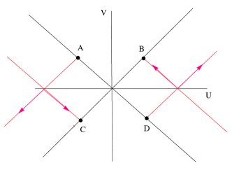
Figure 1: Diagram of the $ERb$ extension (where the origin $(0,0)$ is excluded), showing how the incompleteness of the isotropic geodesics (red lines) may be in principle avoided with a change of topology by gluing points $A\equiv B,C\equiv D$ , and choosing the appropriated light cones orientations.

In the next section we shall use the first identification of points of the $ERb$ manifold ($A\equiv B\,,\,C\equiv D$), and provide the quotient space $ERb/\sim$ with a differentiable structure, obtaining what we have called the hyperbolic Einstein-Rosen bridge. The set formed by all the identified points defines the bridge $B$ connecting the two sheets of the Einstein-Rosen space. The other possible identification of points has been commented by Poplawski POPLA and associated to the extension of the Einstein-Rosen bridge described by Guendelman et al. GUEN1 , which has a $LL$-light brane installed in the bridge.

The following two remarks will help to understand the rest of the paper. Firstly, we must realize that the manifold $ERb/\sim$ obtained by gluing points will have a different differentiable structure than $ERb$. This means that the coordinates to be introduced in a neighbourhood of the bridge $B$ cannot be linked to the coordinates of the $ERb$ manifold of section II by a diffeomorphism. The second remark refers to the orientation of the light cones. Since we are going to identify events $A$ and $B$, if we choose in the region $U>0$ the orientation down-up for the light cone (as shown in Fig. 1), then we must choose the up-down orientation in the region $U<0$, in order to make topologically possible that a light ray can pass through the bridge.

IV A differentiable structure for the quotient space $ERb/\sim$

In order to give a differentiable structure to the quotient space $ERb/\sim$ considered in III.2, we must introduce a system of compatible coordinates covering all the space. We have got it with only a pair of coordinate systems that convert $ERb/\sim$ into a manifold diffeomorphic to the covering space of an hyperboloid of revolution with signature $(-\ +)$. We deviate to the Appendix A the description of this covering space in isothermal coordinates, denoted as $(\bar{U},\bar{V})$, whose values define the set $\bar{H}=\{(\bar{U},\bar{V})\mid\bar{U}^{2}-\bar{V}^{2}>0\,,\bar{U}>0\}$ showed in the right hand of Fig. 2-3. The throat of the hyperboloid generates in the covering space the hyperbola $\bar{J}=\{(\bar{U},\bar{V})\mid\bar{U}^{2}-\bar{V}^{2}=D^{2}\,,\bar{U}>0\}$, which will correspond to the bridge. We start by introducing a map $P_{1}:\Gamma_{1}\subset ERb\,\rightarrow\bar{H}_{1}\subset\bar{H}$, defined on the interior of $ERb$: $\Gamma_{1}=\{(U,V)\in\mathbb{R}^{2}\mid U^{2}-V^{2}>0\}$, and giving values over the covering of the hyperboloid minus the covering of its throat: $\bar{H}_{1}=\{(\bar{U}_{1},\bar{V}_{1})\mid\bar{U}_{1}^{2}-\bar{V}_{1}^{2}>0\,,\bar{U}_{1}>0\}\setminus\bar{J}$. We define it as follows

$$P_{1}(U,V)=(\bar{U}_{1},\bar{V}_{1})$$ (11)

$$\bar{U}_{1}=DS\left(\mathrm{sig}(U)\sqrt{h_{ER}(U^{2}-V^{2})}\right)\frac{\mid U\mid}{\sqrt{U^{2}-V^{2}}}$$ (12)

$$\bar{V}_{1}=DS\left(\mathrm{sig}(U)\sqrt{h_{ER}(U^{2}-V^{2})}\right)\frac{V}{\sqrt{U^{2}-V^{2}}}\ ,$$ (13)

where $D$ is an arbitrary positive constant and $S(\cdot)$ is a positive, smooth and monotonous increasing function verifying $S(0)=1$. The values of this function allow the introduction of the coordinate system $(\bar{U}_{1},\bar{V}_{1})$ over the subset $\Gamma_{1}\subset ERb/\sim$. In Appendix A we prove that, with this definition, the assignation $(\bar{U}_{1},\bar{V}_{1})=(\bar{U},\bar{V})$ is a diffeomorphism between our manifold minus the bridge and the covering of the hyperboloid minus the throat.

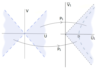
Figure 2: Map $P_{1}:\Gamma_{1}\rightarrow\bar{H}_{1}$. It introduces the coordinates $(\bar{U}_{1},\bar{V}_{1})$ over $ERb/\sim$ excluding the bridge, which is represented as an hyperbola (with point $(D,0)$ removed) in these coordinates.

To complete the differentiable structure we need coordinates for a neighbourhood of the bridge $B$. To this end, we consider the map $P_{2}:\Gamma_{2}\subset ERb\rightarrow\bar{H}_{2}\subset\bar{H}$, with $\Gamma_{2}=\{(U,V)\mid 0\leq U^{2}-V^{2}<\epsilon^{2}\}-(0,0)$, defined as

$$P_{2}(U,V)=(\bar{U}_{2},\bar{V}_{2})=\left(\sqrt{V^{2}+D^{2}}+\frac{U^{2}-V^{2}}{U}\,\ ,V\right)\ .$$ (14)

The bridge $B$ is mapped onto $\bar{J}-(D,0)$, where $\bar{J}$ is the hyperbola defined above. The image set $\bar{H}_{2}=P_{2}(\Gamma_{2})$ is now a neighborhood of the set $\bar{J}-(D,0)$, defined as

$$\bar{H}_{2}=\{(\bar{U}_{2},\bar{V}_{2})\mid\bar{U}_{L}(\bar{V}_{2})<\bar{U}_{2}<\bar{U}_{R}(\bar{V}_{2})\}-(D,0)$$ (15)

$$\bar{U}_{L}(\bar{V}_{2})=\sqrt{\bar{V}_{2}^{2}+D^{2}}-\frac{\epsilon^{2}}{\sqrt{\bar{V}_{2}^{2}+\epsilon^{2}}}\,\ ,\ \bar{U}_{R}(\bar{V}_{2})=\sqrt{\bar{V}_{2}^{2}+D^{2}}+\frac{\epsilon^{2}}{\sqrt{\bar{V}_{2}^{2}+\epsilon^{2}}}\ ,$$ (16)

as shown in the right hand of Fig. 3. This map verifies $P_{2}(-b,b)=P_{2}(b,b)$ and $P_{2}(-b,-b)=P_{2}(b,-b)$ for any $b>0$, i.e, it is not injective over the boundary $\partial ERb$ defined in II. The set $\Gamma_{2}\setminus\partial ERb$ is formed by two disjoint open subsets $\{R_{i}\}_{i=1,2}\subset\Gamma_{2}\setminus\partial ERb$, and $P_{2}$ maps them bijectively onto two open subsets $\{\bar{R}_{i}\}_{i=1,2}\subset\bar{H}_{2}\setminus\ \bar{J}$, i.e, $P_{2}(R_{i})=\bar{R}_{i}$ as shown in Fig. 3. We shall need the coordinates of the sets $R_{i}=P_{2}^{-1}(\bar{R}_{i})$ as functions of the coordinates of $\bar{R}_{i}$. One gets

$$P_{2}^{-1}(\bar{R}_{1})=\{(U_{-},V)\}\,\ \ ,\,\ \ P_{2}^{-1}(\bar{R}_{2})=\{(U_{+},V)\}$$ (17)

$$U_{+}=\frac{1}{2}(\sqrt{\varphi^{2}+4\bar{V}_{2}^{2}}-\varphi)\,\ ,V=\bar{V}_{2}$$ (18)

$$U_{-}=-\frac{1}{2}(\sqrt{\varphi^{2}+4\bar{V}_{2}^{2}}+\varphi)\,\ ,V=\bar{V}_{2}\,\ ,\ \varphi=\sqrt{\bar{V}_{2}^{2}+D^{2}}-\bar{U}_{2}\ .$$ (19)

The non-injectivity of $P_{2}$ over the boundary $\partial ERb$ will make possible to assign the same coordinates to pairs of points like $A,B$ and $C,D$. By identifying the pairs $(-b,b),(b,b)$ and $(-b,-b),(b,-b)$ of the set $\Gamma_{2},$ shown in the left part of Fig. 3, we obtain a neighborhood of the bridge of the quotient space $\mathrm{ERb}/\sim$.

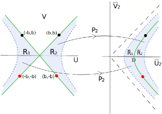
Figure 3: Map $P_{2}:\Gamma_{2}\rightarrow\bar{H}_{2}$. It maps a neighborhood of the bridge $B$, formed by the set of identified points, onto a neighborhood of the covering of the throat of the hyperboloid, represented by the hyperbola in green. The values of this function define the coordinates $(\bar{U}_{2},\bar{V}_{2})$.

With this application we can proceed to the introduction of the coordinate system $(\bar{U}_{2},\bar{V}_{2})$ in a neighborhood $\Gamma_{2}/\sim\,\ \subset ERb/\sim$ of the bridge of the quotient space as follows. To the pair of points $(-V,V)\equiv(V,V)$ we assign coordinates $(\bar{U}_{2},\bar{V}_{2})=(\sqrt{V^{2}+D^{2}},V)$. To points such that $U^{2}-V^{2}>0$ we assign coordinates $(\bar{U}_{2},\bar{V}_{2})=(\sqrt{V^{2}+D^{2}}+\frac{U^{2}-V^{2}}{U},V)$. With the next proposition we shall provide a differentiable structure to the quotient space $ERb/\sim$.

Proposition 2. The coordinate systems $(\bar{U}_{1},\bar{V}_{1})$ and $(\bar{U}_{2},\bar{V}_{2})$ over the quotient space $ERb/\sim$ are compatible, i.e., the function change of coordinates is a diffeomorphism.

To prove it we have to consider the common regions of the domains of $P_{1}$ and $P_{2}$, that is $R_{1}\cup R_{2}$. It is enough to prove it in one of them, since in the other one the procedure would be analogue. We choose $R_{2}$, as shown in Fig. 4. So, we shall choose $U=U_{+}=\frac{1}{2}(\sqrt{\varphi^{2}+4\bar{V}_{2}^{2}}-\varphi),\bar{V}_{2}=V$ given in (18), and we can express $V/U$ and $U^{2}-V^{2}$ as functions of $(\bar{U}_{2},\bar{V}_{2})$

$$\frac{V}{U}=q(\bar{U}_{2},\bar{V}_{2})\,\ ,\ q(\bar{U}_{2},\bar{V}_{2})=\frac{2\bar{V}_{2}}{-\varphi+\sqrt{\varphi^{2}+4\bar{V}_{2}^{2}}}$$ (20)

$$U^{2}-V^{2}=p(\bar{U}_{2},\bar{V}_{2})\,\ ,\ p(\bar{U}_{2},\bar{V}_{2})=\frac{\varphi}{2}\left(\varphi-\sqrt{\varphi^{2}+4\bar{V}_{2}^{2}}\right)\ .$$ (21)

The functions $p(\bar{U}_{2},\bar{V}_{2})$ and $q(\bar{U}_{2},\bar{V}_{2})$ are both differentiable and moreover $|q(\bar{U}_{2},\bar{V}_{2})|<1$ because $\varphi<0$ in the region considered. This property will be used bellow. Let us introduce $\tilde{S}(\bar{U}_{2},\bar{V}_{2})=S\left(\sqrt{h_{ER}(p(\bar{U}_{2},\bar{V}_{2})}\right)$, then from equation (11) we have

$$\bar{U}_{1}^{2}-\bar{V}_{1}^{2}=D^{2}\tilde{S}(\bar{U}_{2},\bar{V}_{2})^{2}$$ (22)

$$\frac{\bar{V}_{1}}{\bar{U}_{1}}=q(\bar{U}_{2},\bar{V}_{2})=\frac{V}{U}\ ,$$ (23)

and by combining (22) and (23) one gets the change of coordinates

$$\bar{U}_{1}=\frac{D\tilde{S}(\bar{U}_{2},\bar{V}_{2})}{\sqrt{1-q(\bar{U}_{2},\bar{V}_{2})^{2}}}\,\ ,\ \bar{V}_{1}=\frac{D\tilde{S}(\bar{U}_{2},\bar{V}_{2})q(\bar{U}_{2},\bar{V}_{2})}{\sqrt{1-q(\bar{U}_{2},\bar{V}_{2})^{2}}}\ .$$ (24)

The change of coordinates (24) is differentiable because $q^{2}<1$ in the domain considered. This completes the proof.

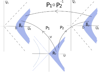
Figure 4: Diagram of the change of isothermic coordinates $(\bar{U}_{2},\bar{V}_{2})\rightarrow(\bar{U}_{1},\bar{V}_{1})$ in the region $R_{2}$, that has been proved to be differentiable.

With the coordinate systems $(\bar{U}_{1},\bar{V}_{1}),(\bar{U}_{2},\bar{V}_{2})$ we cover all the space $\bar{H}=\{(\bar{U},\bar{V})\mid\bar{U}^{2}-\bar{V}^{2}>0\,,\bar{U}>0\}$. Hence we have given a differentiable structure to the quotient space $ERb/\sim$. Regarding the geometrical characteristics of this space, the manifold $ERb/\sim$ is diffeomorphic to the covering space of the hyperboloid of revolution with the point $(D,0)$ removed, as proved in Appendix A. This is why we have given the name hyperbolic Einstein-Rosen bridge (hER) to the manifold $ERb/\sim$. Simply, to a point with coordinates $(\bar{U}_{1},\bar{V}_{1})$ we associate a point of the hyperboloid with the same coordinates $(\bar{U},\bar{V})=(\bar{U}_{1},\bar{V}_{1})$, and similarly for points of $ERb/\sim$ with coordinates $(\bar{U}_{2},\bar{V}_{2})$. Therefore, the set $\bar{J}-(D,0)\subset\bar{H}$, which is the throat of the hyperboloid, is diffeomorphic to the bridge $B\subset ERb/\sim$ that connects the sheets of the Einstein-Rosen space.

In the next section, using the function $P_{2}^{-1}$ introduced in (17) we shall get the metric in a neighborhood of the bridge expressed in coordinates $(\bar{U}_{2},\bar{V}_{2})$, and will be able to study the passability of the bridge.

V The metric on the hyperbolic Einstein-Rosen bridge $hER$

The metric space $(ERb,\Omega^{2}_{ER}\eta)$ with $\eta=-dV^{2}+dU^{2}$, obtained in section II, is a non maximal extension of the incomplete Einstein-Rosen bridge. In the previous section we have obtained, by identifying points of the bridge, a new manifold $ERb/\sim$ which is diffeomorphic to the covering space of an hyperboloid of revolution, and we have provided it with a differential structure. We shall explain how to obtain in this new space a maximal extension of the Einstein-Rosen bridge different from the well-known Kruskal-Szequeres black hole.

The dipheomorphism $P_{2}^{-1}:\bar{R}_{2}\subset\bar{H}_{2}\setminus\bar{J}\rightarrow R_{2}\subset\Gamma_{2}$ will be used now to pullback the metric on the open set $R_{2}\subset\Gamma_{2}$ over the open set $\bar{R}_{2}$. So, taking into account (18), we get

$$dU=Ad\bar{U}_{2}+Bd\bar{V}_{2}\,,\,dV=d\bar{V}_{2}$$ (25)

$$A=\frac{1}{2}\left(1-\frac{\varphi}{\sqrt{\varphi^{2}+4\bar{V}_{2}^{2}}}\right)$$ (26)

$$B=-\frac{1}{2}\left(1-\frac{\varphi}{\sqrt{\varphi^{2}+4\bar{V}_{2}^{2}}}\right)\frac{\bar{V}_{2}}{\sqrt{\bar{V}_{2}^{2}+D^{2}}}+\frac{2\bar{V}_{2}}{\sqrt{\varphi^{2}+4\bar{V}_{2}^{2}}}\ ,$$ (27)

with $\varphi=\sqrt{\bar{V}_{2}^{2}+D^{2}}-\bar{U}_{2}$. Using these relations we get the metric in the region $\bar{R}_{2}\subset\bar{H}_{2}$, where $\varphi<0$, shown in Fig. 3

$$d\bar{s}^{2}=\bar{\Omega}^{2}(\bar{\eta}_{{}_{\bar{U}_{2}\bar{U}_{2}}}d\bar{U}_{2}^{2}+\bar{\eta}_{{}_{\bar{V}_{2}\bar{V}_{2}}}d\bar{V}_{2}^{2}+2\bar{\eta}_{{}_{\bar{U}_{2}\bar{V}_{2}}}d\bar{U}_{2}d\bar{V}_{2})$$ (28)

$$\bar{\eta}_{{}_{\bar{V}_{2}\bar{V}_{2}}}=B^{2}-1\,\ ,\ \bar{\eta}_{{}_{\bar{U}_{2}\bar{U}_{2}}}=A^{2}\,\ ,\,\bar{\eta}_{{}_{\bar{U}_{2}\bar{V}_{2}}}=AB\ ,$$ (29)

where the factor $\bar{\Omega}^{2}=\Omega^{2}_{ER}(U^{2}-V^{2})$ is obtained by substituting $U^{2}-V^{2}=U_{+}^{2}-V^{2}=\frac{\varphi}{2}\left(\varphi-\sqrt{\varphi^{2}+4\bar{V}_{2}^{2}}\right)$into the function $\Omega^{2}_{ER}$ given in (10). The same functional form of the metric defined above in $\bar{R}_{2}$ is extended now to the the region $(\bar{J}-(D,0))\cup\bar{R}_{1}$ where $\varphi\geq 0$. The extended metric is degenerate over the axis $\bar{V}_{2}=0$ in the region $\varphi>0$ (the left hand of the bridge), because there we have $A=B=0$, but it is smooth over all the bridge $\bar{J}-(D,0)$.

The components of the metric are analytic functions in the open set formed by subtracting the semi axis $\varphi>0\,,\bar{V}_{2}=0$ from the open set $\bar{H}_{2}$, and so are the components of the Ricci tensor. On the other hand, by construction, the Ricci tensor is null in the region $\bar{R}_{2}$ (to the right of the bridge), since this region is diffeomorphic to the right hand of the Einstein-Rosen space-time, where the Ricci tensor vanishes. Therefore, according to the theorem of interior uniqueness of analytic functions, the Ricci tensor will also be null in the region $\bar{R}_{1}$ (to the left of the bridge) minus the semi axis $\varphi>0\,,\bar{V}_{2}=0$. Then, the metric verifies the Einstein equations in empty space, except in the degenerate region. To ascertain the geometrical character of the degeneracy we have considered the Kretschmann scalar, $\mathrm{Kret}(\bar{U}_{2},\bar{V}_{2})=R_{abcd}R^{abcd}$ in the region $\varphi>0$, $\bar{U}_{2}<D$, to study the limit when $\bar{V}_{2}$ tends to zero keeping $\bar{U}_{2}$ constant. We have found that it diverges as $(D-\bar{U}_{2})^{6}/\bar{V}_{2}^{10}$. The calculation is straightforward and helped by the fact that the metric is the sum of two mutually independent submetrics. The semi-axis $\varphi>0,\bar{V}_{2}=0$ is therefore a geometrical singularity of the space-time.

We shall show that the bridge is a horizon that protects the right region ($\varphi<0$) from the singularity present in the left region ($\varphi>0$), as in the maximal extension of the Schwarzschild metric. We start studying the geometrical properties of the hyperbola $\bar{J}-(D,0)$. A bridge is the possibility of communicating two separate zones. To ascertain if our hyperbola has this property we shall construct the light cones over it, i.e., the tangent vectors to the pair of light rays at any point of $\bar{J}$. If we renounce to an affine parametrization we can get them by considering the simpler metric $ds^{2}=\bar{\eta}_{{}_{\bar{U}_{2}\bar{U}_{2}}}d\bar{U}_{2}^{2}+\bar{\eta}_{{}_{\bar{V}_{2}\bar{V}_{2}}}d\bar{V}_{2}^{2}+2\bar{\eta}_{{}_{\bar{U}_{2}\bar{V}_{2}}}d\bar{U}_{2}d\bar{V}_{2}$. It is manifest that the transformation $\bar{V}_{2}\rightarrow-\bar{V}_{2}$ is an isometry, therefore the geodesics in the $\bar{V}_{2}<0$ region may be obtained by symmetry respect the $\bar{V}_{2}=0$ axis. Using the coordinate $\bar{V}_{2}$ as parameter of the isotropic geodesics, we get an algebraic equation to determine the isotropic directions, which is given by

$$\bar{\eta}_{{}_{\bar{U}_{2}\bar{U}_{2}}}\left(\frac{d\bar{U}_{2}}{d\bar{V}_{2}}\right)^{2}+2\eta_{{}_{\bar{U}_{2}\bar{V}_{2}}}\frac{d\bar{U}_{2}}{d\bar{V}_{2}}+\bar{\eta}_{{}_{\bar{V}_{2}\bar{V}_{2}}}=0\ .$$ (30)

The two solutions define the following two first order differential equations

$$\frac{d\bar{U}_{2}}{d\bar{V}_{2}}=\frac{1-B}{A}\,\ \ ,\ \ \frac{d\bar{U}_{2}}{d\bar{V}_{2}}=-\frac{1+B}{A}\ ,$$ (31)

where $A$ and $B$ are defined in (26), (27). On the bridge it is verified $\varphi=0$, so we have

$$\frac{1-B}{A}\mid_{\varphi=0}=\frac{\bar{V}_{2}}{\sqrt{\bar{V}_{2}^{2}+D^{2}}}\,\ \ ,\ -\frac{1+B}{A}\mid_{\varphi=0}=\frac{\bar{V}_{2}}{\sqrt{\bar{V}_{2}^{2}+D^{2}}}-4\,\ \mathrm{if}\,\ \bar{V}_{2}>0$$ (32)

$$\frac{1-B}{A}\mid_{\varphi=0}=\frac{\bar{V}_{2}}{\sqrt{\bar{V}_{2}^{2}+D^{2}}}+4\,\ \ ,\ -\frac{1+B}{A}\mid_{\varphi=0}=\frac{\bar{V}_{2}}{\sqrt{\bar{V}_{2}^{2}+D^{2}}}\,\ \mathrm{if}\,\ \bar{V}_{2}<0\ ,$$ (33)

and it follows immediately that the parametrization $(\bar{U}_{2}=\sqrt{\bar{V}_{2}^{2}+D^{2}},\bar{V}_{2}=\bar{V}_{2})$ of the bridge $\bar{J}-(D,0)$ is a light ray. One of the two isotropic vectors at any point $p\in\bar{J}-(D,0)$ is the tangent vector to the bridge $K_{1}=(\frac{\bar{V}_{2}}{\sqrt{\bar{V}_{2}^{2}+D^{2}}},1)$, while the other one is clearly directed from right to left: $K_{2}=(-4+\frac{\bar{V}_{2}}{\sqrt{\bar{V}_{2}^{2}+D^{2}}},1)$ in the $\bar{V}_{2}>0$ region, and from left to right $K_{2}=(4+\frac{\bar{V}_{2}}{\sqrt{\bar{V}_{2}^{2}+D^{2}}},1)$ in the $\bar{V}_{2}<0$ zone . The couple $(K_{1},K_{2})$ define the light cone at each point of the bridge. They show that in the region $\bar{V}_{2}>0$ the matter can traverse the bridge only in right to left direction; by contrary in the region $\bar{V}_{2}<0$ matter only can traverse it from left to right. Therefore we conclude that the bridge is traversable.

Fig. 5 shows the representation of some isotropic geodesics in a neighbourhood of the bridge and the light cones, which show the possible transit directions. These directions agree with the orientation of the light cone chosen at the end of section III.2. Let us point out that if we had started obtaining the metric on $\bar{R}_{1}\subset\bar{H}_{2}$ by choosing the value $U=U_{-}$ given in (19), instead of $U=U_{+}$, and extending it to $\bar{R}_{2}$, the bridge would be passable too but with inverted transit directions. This option would correspond to the opposite choice of the light cone orientation in section (III.2).

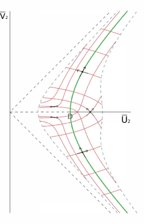
Figure 5: Diagram showing the light rays (red lines) in a neighbourhood of the bridge using coordinates $(\bar{U}_{2},\bar{V}_{2})$. The central hyperbola (green line), minus $(D,0)$, is the bridge formed by two interrupted light rays. The light cones traced on the bridge show the possible directions of transit for light and matter. All the light rays have been obtained using $Mathematica$.

.

Regarding the point $(D,0)$, it is a conical singularity and is not included in the space-time. If it had been included in the new manifold, the metric would be discontinuous at that point, and equations (31) would be of the form $\frac{d\bar{U}_{2}}{d\bar{V}_{2}}=f(\bar{U}_{2},\bar{V}_{2})$ with $f(\bar{U}_{2},\bar{V}_{2})$ discontinuous at $(D,0)$, no satisfying the existence theorem.

An interesting characteristic of the semi-axis $(\varphi>0,\bar{V}_{2}=0)$, where the metric is degenerate, is that it cannot be connected by light rays to any point of the space time, as it is manifest in Fig. 5. Moreover, light and matter coming from the region $\varphi>0,\bar{V}_{2}>0$ cannot traverse to the right side. Therefore, the bridge acts as a horizon and the singularity satisfies the cosmic censorship, since it is causally disconnected from the right side. This singularity could have been avoided by obtaining the metric on the left and right regions (i.e., $\bar{R}_{1}$ and $\bar{R}_{2}$) independently, as pull-backs of the known metrics in regions $R_{1}$ and $R_{2}$. But the metric obtained in this way is not continuous on the bridge, and it cannot be considered an actual extension of the Einstein-Rosen space.

VI The problem of the source of the $hER$ metric space.

Finally, let us add some comments about the source of the $hER$ metric space. According to Katanaev, a point particle is the source of the incomplete metric (1). However, the point particle is at $r=0$ in isotropic coordinates, which is at infinite distance of the bridge where the curvature of this space-time is enormous. This fact is interpreted by Katanaev as repulsive gravity in the left side of the bridge, but for us this is an uncomfortable conclusion that prompts to look for a different interpretation.

In the case of the black-hole extension of the Schwarzschild metric, an illuminating finding was its relation with the continued gravitational contraction of an spherical star made of pressure-less matter OPENSNY : only the exterior of the collapsing star was a part of the Kruskal-Szekeres extension. In our case, it is an interesting issue to find the kind of collapse whose exterior would correspond to a part of the hyperbolic Einstein-Rosen bridge. The spherical star must contract, as shown in Fig. 6, until the free surface reaches the bridge, and then it must begin to expand again, but now in the other side of it. (Only negative pressures could produce this sort of collapse. Newtonian gravity predicts a negative gravitational contribution to the pressure, but a correct extension of this gravitational effect has not been accomplished so far). The orientation of the light cone in Fig. 6 shows that the source in her expansive phase, in the left part of the bridge, can not be observed from the right of it, and no material particle evolving in the left part can get the bridge. In other words, an observer in the right side could not distinguish this process from an Oppenheimer-Snyder collapse creating a black-hole. However, after crossing the horizon, the star would not finish in a singularity, but would begin to expand again. In fact, no singularities would be present, since the degenerate region $(\bar{U}_{2}<D,\bar{V}_{2}=0)$ is now occupied by the collapsing fluid.

This interpretation would explain why gravity is stronger on the bridge, because any point of it is connected by a light ray (the bridge) to the collapsing body at the point of maximum contraction. By contrast, the curvature tends to zero at great distances to the left of the bridge, because the light rays connect with points at the expansion phase. No point-particle would be present in this space-time, only a part of the mathematical point-particle Katanaev’s solution would be generated as the exterior of this collapse-expansion process.

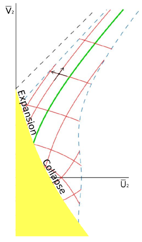
Figure 6: Diagram of the proposed collapse process generating a part of the $hER$ space-time. The green line represents the bridge, generated by light rays. The yellow region is the source, contracting before and in expansion after passing the bridge.

VII Conclusions

In this work we have obtained a new extension ($hER$) of the original incomplete Einstein-Rosen bridge, different from the well-known Kruskal-Szekeres space-time and from the more recent one obtained by Guendelman et al. GUEN1 ; GUEN2 . The manifold of $hER$ is diffeomorphic to the covering space of an hyperboloid of revolution, and the metric components are analytic functions in a neighborhood of the bridge with a geometrical singularity on the semi axis $\bar{V}_{2}=0,\bar{U}_{2}<D$. The bridge is formed by light rays, and is traversable unlike the bridge in the $KS$ extension. The $hER$ space-time differs from the one obtained by Guendelman et al. in three aspects: a) it has no source installed in the bridge, b) it has no closed time-like geodesics typical of whormholes with exotic sources, and c) it presents a singularity, though compatible with the cosmic censorship conjecture (it is causally disconnected from the opposite side of the bridge, so the bridge acts as a horitzon). Finally, we have discussed the problem of the source of this space-time, and proposed a gravitational collapse as in the black-hole case but with two phases: contraction in one side and expansion in the other. It would generate a part of the $hER$ metric in the exterior of the collapse, avoiding the singularity. We leave the deep analysis of this process for future work.

Acknowledgments.– P. B. is supported by a Ph.D. fellowship, Grant No. FPU17/03712. M.P. thanks support by the Spanish ”Ministerio de Economia y Competitividad (sic)” and the ”Fondo Europeo de Desarrollo Regional” MINECO-FEDER Project No. PGC2018-095251-B.100.

Appendix A: Diffeomorphism with the covering space of the hyperboloid

We shall obtain the expression in isothermal coordinates of the covering space of a two dimensional hyperboloid with signature $(-,+)$ that has been used in section IV. The manifold of the two-dimensional sections with ($\theta,\varphi$) constant of the Einstein-Rosen metric given in (1) could be considered, excluding the section $u=0$, as a surface of revolution (for example the one sheet hyperboloid) if we take $t$ as the angle of revolution. This is only possible if we consider the covering space of the hyperboloid, $\bar{H},$ by extending to all $\mathbb{R}$ its angular coordinate, defined in $(0,2\pi)$. We shall do that and our quotient space $ERb/\sim$ defined in section IV will be diffeomorphic to the covering surface $\bar{H}$.

Description of a one sheet hyperboloid with signature $(-\,\ +)$. We consider in the space $\mathbb{R}^{3}$ the metric $ds^{2}=-dx^{2}-dy^{2}+dz^{2}$, and the surface of an hyperboloid defined by $\frac{x^{2}}{q^{2}}+\frac{y^{2}}{q^{2}}-\frac{z^{2}}{p^{2}}=1$, with $p>q$. It can be parametrizated as: $X(\varphi_{1},\varphi_{2})=(q\cosh\varphi_{2}\cos\varphi_{1},q\cosh\varphi_{2}\sin\varphi_{1},p\sinh\varphi_{2})$, with $0<\varphi_{1}<2\pi\,,\ -\infty<\varphi_{2}<\infty$, and one obtains the metric $ds^{2}=-q^{2}\cosh^{2}\varphi_{2}\,d\varphi_{1}^{2}+(p^{2}\cosh^{2}\varphi_{2}-q^{2}\sinh^{2}\varphi_{2})d\varphi_{2}^{2}$. Now, using the Proposition 1 we can introduce isothermal coordinates $\bar{U}=f_{{H}}(\varphi_{2})\cosh(\varphi_{1})$, $\bar{V}=f_{{H}}(\varphi_{2})\sinh(\varphi_{1})$, with $f_{H}(\varphi_{2})=D\exp(\int_{0}^{\varphi_{2}}\sqrt{1-\frac{p^{2}}{q^{2}}\tanh^{2}s}\,ds)$ and $D$ a positive arbitrary constant, and express the metric as $d\bar{s}^{2}=q^{2}\cosh^{2}(\varphi_{2})f_{H}^{-2}(\varphi_{2})(-d\bar{V}^{2}+d\bar{U}^{2})$. The equation $\bar{U}^{2}-\bar{V}^{2}=f_{H}^{2}(\varphi_{2})$ defines a monotonous increasing function, $\varphi_{2}=h_{{}_{H}}(\bar{U}^{2}-\bar{V}^{2})$ in the open set $\bar{U}^{2}-\bar{V}^{2}>0,\bar{U}>0$. It verifies: $h_{H}(0)=-\infty\,,\ h_{H}(D^{2})=0\,,\ h_{H}(\infty)=\infty$. In isothermal coordinates, the lines $\varphi_{1}=\mathrm{const}.$ in the $(\varphi_{1},\varphi_{2})$ plane transform into the straight lines $\bar{V}=\tanh(\varphi_{1})\,\bar{U}$ in the $(\bar{U},\bar{V})$ plane, for values $0<\varphi_{1}<2\pi$; and the circles $\varphi_{2}=\mathrm{const}.$ into segments of the hyperbolae $\bar{U}^{2}-\bar{V}^{2}=f_{H}^{2}(\varphi_{2})$. In particular, the circle $\varphi_{2}=0$ transforms into a segment of the hiperbola $\bar{J}=\{(\bar{U},\bar{V})\mid\bar{U}^{2}-\bar{V}^{2}=D^{2},\bar{U}>0\}$ in isothermal coordinates.

The covering space $\bar{H}$ of the one sheet hyperboloid. The covering space of a circle in $\mathbb{R}^{2}$, parametrized as $X(\varphi_{1},\varphi_{2})=(a\cos\varphi_{1},a\sin\varphi_{1})$, is the helix in $\mathbb{R}^{3}$, parametrized as $X(\varphi_{1},\varphi_{2})=(a\cos\varphi_{1},a\sin\varphi_{1},b\varphi_{1})$. Using this analogy we extend the coordinate $\varphi_{1}$ to obtain the parametrization of the covering space of the one sheet hyperboloid: $X(\varphi_{1},\varphi_{2})=(q\cosh\varphi_{2}\cos\varphi_{1},q\cosh\varphi_{2}\sin\varphi_{1},p\sinh\varphi_{2},\ \varphi_{1})$, with $-\infty<\varphi_{1}<\infty\,,\ -\infty<\varphi_{2}<\infty$. The expression in isothermal coordinates of this covering space can be obtained by extending the range of values of the isothermal coordinates of the hyperboloid to the open set $\bar{H}=\bar{U}^{2}-\bar{V}^{2}>0\,,\bar{U}>0$.

Diffeomorphism $ERb/\sim\,\leftrightarrow\bar{H}-(D,0)$. We start with the non isothermal coordinates $(u,t),(\varphi_{2},\varphi_{1})$, used to express the Einstein-Rosen metric (1) and the covering space of the one sheet hyperboloid respectively. Let us consider the following diffeomorphisms: $\varphi_{2}=u\,,\,\varphi_{1}=\frac{t}{4m}$, for the open $u>0$ and $\varphi_{2}=u\,,\,\varphi_{1}=-\frac{t}{4m}$ for the open $u<0$. Now, by considering the inverse change $u=\mathrm{sig}(U)\sqrt{h_{ER}(U^{2}-V^{2})}$ (see section II) and the well-known hyperbolic trigonometric relations, we get the expressions of this assignations in isothermal coordinates

$$\bar{U}=f_{H}\left(\mathrm{sig}(U)\sqrt{h_{ER}(U^{2}-V^{2})}\right)\frac{\mid U\mid}{\sqrt{U^{2}-V^{2}}}\,\,\,$$ (34)

$$\bar{V}=f_{H}\left(\mathrm{sig}(U)\sqrt{h_{ER}(U^{2}-V^{2})}\right)\frac{V}{\sqrt{U^{2}-V^{2}}}\ .$$ (35)

Note that they coincide with the expressions of the map $P_{1}$, given by (11), if we define $S=f_{H}/D$. If we had chosen a different surface of revolution diffeomorphic to the hyperboloid, we would had obtained a different function $S(\cdot)$ with similar characteristics. That is why in the definition of $P_{1}$ we have generalized the function $S(\cdot)$ to any positive, smooth and monotonous increasing function verifying $S(0)=1$. Therefore, any point of the manifold $ERb/\sim$ defined with the coordinates $(\bar{U}_{1},\bar{V}_{1})$ (all points except the bridge), can be related with the hyperboloid (or a similar surface of revolution) by the diffeomorphism $\bar{U}_{1}=\bar{U}\,,\,\bar{V}_{1}=\bar{V}$, covering all the surface except the throat $\bar{J}$. The points of the bridge (and its neighbourhood) in the manifold $ERb/\sim$ can be expressed with the coordinates $(\bar{U}_{2},\bar{V}_{2})$, defined in (14). The bridge correspond to the set $B=\{(\bar{U}_{2},\bar{V}_{2})\mid\bar{U}_{2}^{2}-\bar{V}_{2}^{2}=D^{2}\,,\bar{U}_{2}>0\}-(D,0)$, so it can be related to the throat of the hyperboloid by the simple diffeomorphism $\bar{U}_{2}=\bar{U}\,,\,\bar{V}_{2}=\bar{V}$. In the Proposition 2 we have proved that the coordinate systems $(\bar{U}_{1},\bar{V}_{1})$ and $(\bar{U}_{2},\bar{V}_{2})$ are compatible in the intersection of their domains, so there are no discontinuities. Therefore the manifold $ERb/\sim$ is diffeomorphic to the covering space of the one sheet hyperboloid $\bar{H}$, after removing the point $(D,0)$.

Appendix B: Definitions

We shall summarize the main definitions used in the paper in order to facilitate the reading.

$ERb=\{(U,V)\in\mathbb{R}^{2}\mid U^{2}-V^{2}\geq 0\}-(0,0)$

$\partial ERb=\{(U,V)\in\mathbb{R}^{2}\mid U^{2}-V^{2}=0\}-(0,0)$

$R_{1}\subset ERb=\{(U,V)\in\mathbb{R}^{2}\mid 0<U^{2}-V^{2}<\epsilon^{2},U<0\}\}$

$R_{2}\subset ERb=\{(U,V)\in\mathbb{R}^{2}\mid 0<U^{2}-V^{2}<\epsilon^{2},U>0\}\}$

$\Gamma_{1}\subset ERb\,,\,\Gamma_{1}=\{(U,V)\in\mathbb{R}^{2}\mid 0<U^{2}-V^{2}\}$

$\Gamma_{2}\subset ERb\,,\,\Gamma_{2}=\{(U,V)\in\mathbb{R}^{2}\mid 0\leq U^{2}-V^{2}<\epsilon^{2}\}-(0,0)$

$\bar{H}=\{(\bar{U},\bar{V})\in\mathbb{R}^{2}\mid\bar{U}^{2}-\bar{V}^{2}>0\,,\bar{U}>0\}$

$\bar{J}\subset\bar{H}=\{(\bar{U},\bar{V})\in\mathbb{R}^{2}\mid\bar{U}^{2}-\bar{V}^{2}=D^{2}\,,\bar{U}>0\}$

$\bar{H}_{1}\subset\bar{H}\,,\,\bar{H}_{1}=\{(\bar{U}_{1},\bar{V}_{1})\in\mathbb{R}^{2}\mid\bar{U}_{1}^{2}-\bar{V}_{1}^{2}>0\,,\bar{U}_{1}>0\}\setminus\bar{J}$

$\bar{H}_{2}\subset\bar{H}\,,\ \bar{H}_{2}=\{(\bar{U}_{2},\bar{V}_{2})\in\mathbb{R}^{2}\mid\bar{U}_{L}(\bar{V}_{2})<\bar{U}_{2}<\bar{U}_{R}(\bar{V}_{2})\}-(D,0)$

$P_{1}:\Gamma_{1}\subset ERb\rightarrow\bar{H}_{1}\subset\bar{H}$

$P_{2}:\Gamma_{2}\subset ERb\rightarrow\bar{H}_{2}\subset\bar{H}$

$\bar{R}_{1}=\{(\bar{U}_{2},\bar{V}_{2})\in(\bar{H}_{2}-\bar{J})\mid\bar{U}_{2}<\sqrt{D^{2}+\bar{V}_{2}^{2}}\}$

$\bar{R}_{2}=\{(\bar{U}_{2},\bar{V}_{2})\in(\bar{H}_{2}-\bar{J})\mid\bar{U}_{2}>\sqrt{D^{2}+\bar{V}_{2}^{2}}\}$

$P_{2}(R_{i})=\bar{R}_{i}\,,\ i=1,2$

$\varphi=\sqrt{\bar{V}_{2}^{2}+D^{2}}-\bar{U}_{2}$

References

• (1) A. Einstein, E. Rosen, Phys. Rev. 48, 73 (1935).
• (2) M. Katanaev, Gen. Relativ. Grav. 45, 1861 (2013).
• (3) M. Katanaev, Mod. Phys. Lett. A 29, 1450090 (2014).
• (4) E. I. Guendelman, A. Kaganovich, A. E. Nissimov, F. Pacheva, Cent. Eur. J. Phys. 7, 668 (2009).
• (5) E. I. Guendelman, A. E. Nissimov, F. Pacheva, M. Stoilov, Bulg. J. Phys. A 25, 1405 (2017).
• (6) J. Earman, Bangs, Crunches, Whimpers, and Shrieks: Singularities and Acausalities in Relativistic Spacetimes, Oxford University Press, Oxford, England (1995).
• (7) M. D. Kruskal, Phys. Rev. 119, 1743 (1960).
• (8) N. J. Poplawski, Phys. Lett. B 687, 110 (2010).
• (9) Ch. W. Misner, K. S. Thorne, J. A. Wheeler, Gravitation, WH Freeman & Company, San Francisco (2003).
• (10) W. Rindler, Phys. Rev. Lett. 15, 1001 (1965).
• (11) J. R. Oppenheimer, H. Snyder, Phys Rev. 56, 455 (1939).