The Conformal Bootstrap: Theory, Numerical Techniques, and Applications

Abstract

Conformal field theories have been long known to describe the fascinating universal physics of scale invariant critical points. They describe continuous phase transitions in fluids, magnets, and numerous other materials, while at the same time sit at the heart of our modern understanding of quantum field theory. For decades it has been a dream to study these intricate strongly coupled theories nonperturbatively using symmetries and other consistency conditions. This idea, called the conformal bootstrap, saw some successes in two dimensions but it is only in the last ten years that it has been fully realized in three, four, and other dimensions of interest. This renaissance has been possible both due to significant analytical progress in understanding how to set up the bootstrap equations and the development of numerical techniques for finding or constraining their solutions. These developments have led to a number of groundbreaking results, including world record determinations of critical exponents and correlation function coefficients in the Ising and $O(N)$ models in three dimensions. This article will review these exciting developments for newcomers to the bootstrap, giving an introduction to conformal field theories and the theory of conformal blocks, describing numerical techniques for the bootstrap based on convex optimization, and summarizing in detail their applications to fixed points in three and four dimensions with no or minimal supersymmetry.

I Introduction

For most physical systems, the first step to qualitative understanding is to identify their characteristic scales (length, energy, etc.), through which everything else can be expressed via approximate dimensional analysis. However, there exist theories for which this familiar approach does not work, and which are therefore harder to understand intuitively. These are scale invariant theories, which by definition look the same at all distances and energies, and hence do not possess any characteristic scales.

Scale invariant theories are important in physics, because they arise naturally in the theory of critical phenomena. One experimental manifestation of scale invariance in critical phenomena is critical opalescence, first observed near the critical point of CO₂ by Andrews (1869), and interpreted as a sign of density fluctuations occurring over many distance scales by Smoluchowski (1908). The exact solution of the two-dimensional (2d) Ising model by Onsager (1944) also made it possible to see the emergence of scale invariance at the ferromagnet-paramagnet critical point. Nowadays it is understood that all critical points are described by scale invariant theories. This has been incorporated into Wilson’s renormalization group (RG) theory of phase transitions, introduced in Wilson and Kogut (1974) and Wilson (1983), according to which continuous phase transitions are described by the fixed points of RG flows, and are therefore scale invariant.

Formally, scale invariance is expressed as invariance under a rescaling (dilatation) of all coordinates by a uniform factor $x\to\lambda x$. Another interesting class of transformations of space are conformal transformations, defined as transformations preserving angles. Thus conformal transformations are required to look locally at each point as a rotation accompanied by a dilatation, although the rescaling factor can be $x$-dependent. Conformal transformations have been studied by mathematicians since the 19th century Monge (1850). They first entered into physics when Bateman (1910) and Cunningham (1910) showed that Maxwell’s equations are conformally invariant (they are also trivially scale invariant because of the masslessness of the photon).

With conformal invariance being thus a natural extension of scale invariance, one may wonder if scale invariant theories describing critical points in fact possess full conformal invariance. That this should be the case was first conjectured by Polyakov (1970). Since then several theoretical arguments have been given for why scale invariance should generically imply conformal invariance. By now it is understood that most physically relevant scale invariant theories are conformally invariant, and hence referred to as ‘Conformal Field Theories’, or CFTs.

In addition to their role in the theory of critical phenomena, CFTs are also extremely important for the study of quantum field theories (QFTs). For this discussion QFTs may be Euclidean $d$-dimensional field theories, relevant for statistical physics, or field theories in Lorentzian signature, which are relevant for high-energy physics and quantum condensed matter. From the modern perspective, large classes of QFTs can be seen as RG flows which emerge from one CFT (called the UV fixed point) at short distances and flow to either another nontrivial CFT (called the IR fixed point) or a massive phase at long distances. In this sense CFTs can be called signposts in the space of general QFTs. The quest to classify and solve CFTs is a major goal of modern theoretical physics.

The study of CFTs was initiated in the late 1960s, focusing mostly on formal properties of these theories. This early work was done in general dimension $d$, where the group of conformal transformations is finite dimensional, while it is infinite-dimensional in $d=2$ where any holomorphic map gives rise to a conformal transformation. The importance of this special case was realized by Belavin et al. (1984). Using the infinite-dimensional conformal symmetry, they solved the 2d minimal models—an infinite sequence of CFTs describing the critical points of the 2d Ising model and other lattice models such as the 3-state Potts model.

Of course many 2d models can be exactly solved directly on the lattice Baxter (1989), starting with the above-mentioned Onsager solution of the 2d Ising model. The approach of Belavin et al. (1984) was different in that it allowed for a solution of critical theories using the constraints of conformal symmetry alone, with minimal or no microscopic input. The crucial idea to find these solutions was the conformal bootstrap, first described by Ferrara et al. (1973b) and Polyakov (1974). The conformal bootstrap combines conformal invariance with the existence of the operator product expansion (OPE), another powerful concept going back to Wilson (1969) and Kadanoff (1969). This leads to mathematical consistency conditions on the CFT parameters, which were enough to solve the 2d minimal models.

Following these developments, CFT has become an indispensable tool in the theory of 2d critical phenomena. On the other hand, applications of the conformal bootstrap in higher dimensions lagged behind. For example, 3d continuous phase transitions are traditionally studied using the RG by starting from a microscopic action and looking for a fixed point. Often the 3d fixed point of interest is strongly coupled, requiring one to deform the theory artificially in order to do perturbation theory in a small parameter, with the large-$N$ expansion (see e.g. Moshe and Zinn-Justin (2003) for a review) and the $\epsilon$-expansion Wilson and Fisher (1972) being two prime examples. While these theoretical approaches have undoubtedly scored some successes in describing the experimental data, one may wonder what a fully nonperturbative approach such as the conformal bootstrap has to say about this problem.

A period of renewed interest in the conformal bootstrap started following Rattazzi et al. (2008). This work proposed a numerical method, based on linear programming, which made it possible to extract concrete predictions from the conformal bootstrap equations. The method was applicable in higher dimensions (as well as in 2d). Also, an advantage of the method was that rigorous predictions could be extracted without having to fully solve the equations. Since then the method was greatly improved and many interesting results were obtained, mostly for conformal field theories in 3d and 4d, but also in other dimensions. One flagship result of this line of research is the world’s most precise determination of the critical exponents of the critical 3d Ising model (see Kos et al. (2016) for the current world record results). Our purpose is to review these developments, focusing on applications to the most interesting 3d and 4d CFTs considered so far, as well as to give an overview of the theoretical and numerical techniques which proved useful for these applications.

I.1 Outline

Due to the overwhelming number of results in various incarnations of the conformal bootstrap, our review will necessarily be limited in scope. Let us briefly outline the topics that we will cover. We begin in Sec. II with an informal overview of the conformal bootstrap. Sec. III provides a concise introduction to the conformal field theory techniques that are needed to set up the bootstrap in $d$ dimensions. We follow in Sec. IV with an overview of the various numerical methods that have been employed in studies of the bootstrap. Secs. V and VI review results obtained from applying these methods to 3d and 4d CFTs. Sec. VII reviews results obtained with the stronger assumptions of 4d $\mathcal{N}=1$ or 3d $\mathcal{N}=2$ superconformal symmetry. We comment on applications to nonunitary models in Sec. VIII. Notably absent from our main review are CFTs in other dimensions (e.g., $d=2$ or $d>4$), CFTs with extended supersymmetry, analytical progress in the bootstrap, logarithmic and nonrelativstic CFTs, and other related topics. We finish with a brief overview of progress in these related lines of research in Sec. IX and give some concluding words in Sec. X.

II Conformal bootstrap: informal overview

In this section we will give a brief outline of the conformal bootstrap approach to critical phenomena in $d$ dimensions. We will be rather informal in this section, while in the subsequent sections the same material will be treated in more depth and at a higher level of rigor. For another short introduction to these matters, see Poland and Simmons-Duffin (2016). For longer pedagogical introductions see Rychkov (2016b); Simmons-Duffin (2017b).

As a simple physical setup where these methods would be applicable, we can consider a statistical physics system in $d$ spatial dimensions which is (a) in thermodynamic equilibrium and (b) at a temperature corresponding to a continuous phase transition (so that the correlation length is infinite). Suppose that we are interested in equal-time correlation functions of some local quantities characterizing this system:

$$\langle{\cal O}_{1}(x_{1})\ldots{\cal O}_{n}(x_{n})\rangle\,,$$ (1)

where $x_{i}$ are positions in $\mathbb{R}^{d}$. For example, one can think of the 3d Ising model at the critical point, with ${\cal O}_{i}(x)$ the local magnetization, local energy density, etc. In general, the ${\cal O}_{i}(x)$ are called local operators.

We are interested in the behavior of the correlators (1) at distances large compared to any microscopic (such as lattice) scale $a$. According to Wilson’s RG theory, continuous phase transitions are fixed points of RG flows, which means that the long-distance behavior of (1) will have scale invariance (as well as rotation and translation invariance). Using scale invariance, we can formally extend the long-distance behavior of these correlators from distances $|x_{i}-x_{j}|\gg a$ to arbitrary short distances. In what follows we work in the so-defined continuous limit theory, which is exactly scale invariant at all distances from $0$ to $\infty$.

As discussed in the introduction, we expect that the critical theory is also conformally invariant (i.e., a CFT). This means that for any conformal transformation of $d$-dimensional space $x\to x^{\prime}$ (see Sec. III.1 for the definition), Eq. (1) is related to the same correlation function evaluated at points $x_{1}^{\prime},\ldots,x_{n}^{\prime}$. This invariance property (or covariance) of correlation functions is expressed as a transformation rule for local operators, in the next section appearing in Eq. (III.2). For scalar operators, we have

$${\cal O}(x^{\prime})=\Omega(x)^{-\Delta_{\cal O}}{\cal O}(x)\,,$$ (2)

where $\Omega(x)=|\partial x^{\prime}/\partial x|^{1/d}$ is the $x$-dependent scale factor of the conformal transformation, and $\Delta_{\cal O}$ is a fixed parameter characterizing the operator ${\cal O}$, called its scaling dimension.

Polyakov (1970) noticed that invariance under (2) strongly restricts two-point (2pt) and three-point (3pt) correlation functions. The 2pt function is nonzero only for identical operators and can be normalized to one:

$$\langle{\cal O}_{i}(x_{1}){\cal O}_{j}(x_{2})\rangle=\delta_{ij}{|x_{1}-{x_{2}}|^{-2\Delta_{i}}}\,,$$ (3)

while the 3pt function is fixed up to a numerical coefficient:

$$\langle{\cal O}_{1}(x_{1}){\cal O}_{2}(x_{2}){\cal O}_{3}(x_{3})\rangle=\frac{\lambda_{123}}{|x_{12}|^{h_{123}}|x_{13}|^{h_{132}}|x_{23}|^{h_{231}}}\,,$$ (4)

where $x_{ij}\equiv x_{i}-x_{j}$ and $h_{ijk}\equiv\Delta_{i}+\Delta_{j}-\Delta_{k}$. Similar equations hold for operators with indices, see Sec. III.3.

The set of numerical parameters $\Delta_{i}$ and $\lambda_{ijk}$ appearing in (3) and (4) is called the CFT data. It turns out that the CFT data determine not only 2pt and 3pt functions, but are also sufficient to compute all local observables in CFTs in flat space, by which we mean all correlation functions of local operators, including four-point (4pt) and higher-order correlation functions.

To see this, one uses the OPE, which says that we can replace the insertion of two nearby local operators inside a correlation function by a series of single local operators:

$${\cal O}_{i}(x_{1}){\cal O}_{j}(x_{2})=\sum_{k}f_{ijk}{\cal O}_{k}(y)\,.$$ (5)

The coefficients of the series $f_{ijk}$ may and will depend on the relative positions of the operators ${\cal O}_{i}$, ${\cal O}_{j}$, ${\cal O}_{k}$, and on their quantum numbers. Crucially, however, these coefficients are not supposed to depend on which other operators appear in the correlation function, as long as they are sufficiently far away from $x_{1},x_{2},y$. The precise criterion in the CFT context will be given in Eq. (7).

Notice the freedom in where we put operators appearing on the r.h.s. of the OPE: we can choose $y={\textstyle\frac{1}{2}}(x_{1}+x_{2})$, $y=x_{1}$, or any other point nearby. Different choices of $y$ can be related by Taylor-expanding ${\cal O}_{k}$, and thus can be compensated by changing the coefficients of derivatives of ${\cal O}_{k}$ in the OPE. In what follows we will group the operator ${\cal O}_{k}$ together with all its derivatives, formally thinking of $f_{ijk}$ as an infinite power series in $\partial_{y}$.

There are two things that make OPE in conformal field theories more powerful than in a generic QFT. Firstly, compatibility of the OPE with conformal invariance determines the functions $f_{ijk}$ up to a numerical prefactor, coinciding with the 3pt function coefficient $\lambda_{ijk}$ (for this reason it is also called an OPE coefficient):

$$f_{ijk}(x_{1},x_{2},y,\partial_{y})=\lambda_{ijk}\hat{f}_{ijk}(x_{1},x_{2},y,\partial_{y})\,.$$ (6)

The reduced functions $\hat{f}_{ijk}$ depend only on the operator dimensions $\Delta_{i},\Delta_{j},\Delta_{k}$, the spins of these operators (which are kept implicit in this informal discussion), and on the space dimension $d$.

Secondly, the OPE in conformal theories has a finite radius of convergence, which is determined by the distance to the next operator insertions. For example, in the correlator of Eq. (8) given below, the OPE will converge if

$$|x_{1}-y|,\,|x_{2}-y|<\min_{i=3\ldots n}|x_{i}-y|\,,$$ (7)

i.e. if there exists a sphere centered at $y$ and separating $x_{1}$, $x_{2}$ from any other operator insertion.

Because of these two reasons we can compute any correlation function recursively using the OPE, provided that we know the CFT data. For example, suppose we want to compute the $n$-point function

$$\langle{\cal O}_{1}(x_{1}){\cal O}_{2}(x_{2}){\cal O}_{3}(x_{3})\ldots{\cal O}_{n}(x_{n})\rangle\,.$$ (8)

Applying the OPE to ${\cal O}_{1}(x_{1}){\cal O}_{2}(x_{2})$, we reduce this correlator to a sum of correlators containing $n-1$ operators

$$\langle{\cal O}_{k}(y){\cal O}_{3}(x_{3})\ldots{\cal O}_{n}(x_{n})\rangle\,.$$ (9)

Proceeding in this way, we will eventually get down to 2pt functions, which are determined by the CFT data. The only parameters which will enter this computation are the operator positions and quantum numbers, the CFT data, and the space dimension $d$.

Consider now the case of a 4pt function (Eq. (8) with $n=4$) and compute it in two different ways. The first way is to apply the OPE to the pairs of operators ${\cal O}_{1}{\cal O}_{2}$ and ${\cal O}_{3}{\cal O}_{4}$. This reduces the 4pt function to an infinite sum of 2pt functions of operators which appear in these OPEs. A second way is to apply the OPE to the pairs ${\cal O}_{1}{\cal O}_{4}$ and ${\cal O}_{2}{\cal O}_{3}$. Since we are dealing with the same 4pt function, the two expansions must agree in their overlapping regions of convergence. This crossing relation represents a consistency condition on the CFT data and is illustrated in Fig. 1.

The main idea of the conformal bootstrap is that by imposing the crossing relation, we should be able to significantly winnow down the set of all possible CFT data. In the subsequent sections of this review, we will see how the crossing relation can be written in a mathematically manageable form, and how numerical algorithms can be applied to extract from it concrete constraints.

Ideally, if we impose crossing relations for all 4pt functions of the theory, we will be left with the CFT data corresponding to the actually existing critical theories. In practice, it has so far been possible to impose crossing relations on only a handful of 4pt functions at a time. However, we will see that even this limited procedure produces nontrivial constraints, which are in some cases surprisingly strong.

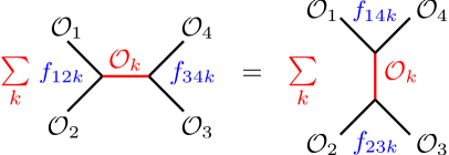
Figure 1: Crossing relation for the 4pt function $\langle{\cal O}_{1}{\cal O}_{2}{\cal O}_{3}{\cal O}_{4}\rangle$.

II.1 Universality and the role of microscopic input

A fundamental concept in the theory of critical phenomena is universality: all continuous phase transitions can be grouped into universality classes which share the same critical exponents. This is neatly explained in Wilson’s RG theory: two phase transitions will fall into the same universality class if they are described by the same fixed point. On the other hand, the conformal bootstrap provides a different perspective on the same phenomenon: each universality class corresponds to a different CFT, with a different set of CFT data.

These two points of view are clearly complementary, and it is important to establish the correspondence between them. Consider for example the critical exponents. In RG theory they can be related to the eigenvalues $\lambda^{y_{i}}$ of the RG transformation linearized around the fixed point, where $\lambda>1$ is the RG rescaling factor. As is well known, these eigenvalues are simply related to the scaling dimensions of the local operators: $y_{i}=d-\Delta_{i}$. Thus, information about the critical exponents can be easily extracted from CFT data, and agreement of their values between an RG fixed point and a CFT may give us confidence that the two describe the same critical universality class.

There are however three more fundamental structural characteristics which can be used to identify universality classes, even before considering the numerical values of critical exponents. These characteristics may not be sufficient to uniquely classify the different CFTs, but they will give us a convenient starting point.

1. The global (or internal) symmetry group. It can be discrete, as for the $\mathbb{Z}_{2}$ symmetry of the Ising model, or continuous, as for the $O(N)$ models. In RG studies, the global symmetry group is specified by considering an RG flow in the space of microscopic theories described by an action possessing a given symmetry. The global symmetry group for a CFT is the same group $G$ as for the corresponding RG fixed point, although it is specified in a different way: by demanding that each local operator transform in an irreducible representation of $G$ and that OPE coefficients respect this symmetry structure.

We note in passing that unlike the global symmetry, the presence of a gauge symmetry in a microscopic description does not manifest itself in the conformal bootstrap, because physically observable local CFT operators are gauge invariant.

2. The number of relevant singlet scalars. The number of scalar operators which are relevant (i.e., have dimension $\Delta_{i}<d$) and transform as singlets under the global symmetry determines whether the universality class has critical as opposed to multicritical behavior. This will be discussed in more detail in Sec. V.1. Here it suffices to note that this number is easy to identify from both the RG and CFT perspectives.

3. Unitarity. Unitarity is of course a required property when quantum mechanics is involved, which is the case for theories of interest to high-energy physics and quantum condensed matter. Many universality classes of interest to statistical physics also happen to be unitary. Importantly, the existence of unitarity can be established at the microscopic scale, and is then inherited by the RG fixed point. In the CFT description, unitarity is imposed via lower bounds on the operator dimensions and reality constraints on the OPE coefficients, see Sec. III.5.

Finally, let us comment on the OPE coefficients $\lambda_{ijk}$. From the CFT point of view, they are an integral part of the CFT data, on par with the scaling dimensions. In the conformal bootstrap approach, the crossing relation involves both $\lambda_{ijk}$ and $\Delta_{i}$. In the examples below, when we are able to determine the $\Delta_{i}$’s to some accuracy (as for the 3d Ising and the $O(N)$ models), we can typically determine the $\lambda_{ijk}$’s to a comparable accuracy. This can be contrasted with the RG approach, where the OPE coefficients do not appear to play such a fundamental role, and they have received relatively little attention.

III Conformal field theory techniques in $d$ dimensions

In this section we review the theory techniques that form the backbone of the conformal bootstrap. These include conformal symmetry, operators and their correlation functions, unitarity and reflection positivity, conformal blocks, and the way they enter crossing relations (also in the presence of global symmetries).

III.1 Conformal transformations

The content of this section is standard textbook material. We will only mention a few fundamental results and set up our conventions. For more details see e.g. Rychkov (2016b); Simmons-Duffin (2017b).

We consider CFTs in flat Euclidean or Lorentzian space with coordinates $x^{\mu}$ and metric $\eta_{\mu\nu}$. Conformal transformations are diffeomorphisms $x\to x^{\prime}$ which locally look like a rotation $\Lambda^{\mu}{}_{\nu}(x)$ combined with a rescaling $\Omega(x)\geqslant 0$ (also called a dilatation), which means that the Jacobian takes the form

$$\frac{\partial x^{\prime\mu}}{\partial x^{\nu}}=\Omega(x)\Lambda^{\mu}{}_{\nu}(x),\quad\eta_{\rho\sigma}\Lambda^{\rho}{}_{\mu}(x)\Lambda^{\sigma}{}_{\nu}(x)=\eta_{\mu\nu}\,.\qquad$$ (10)

Alternatively, the same condition can be expressed by saying that the transformation preserves angles, or that it leaves the metric invariant up to an overall factor.

In any dimension $d\geqslant 3$, the case of primary interest for this review, a theorem of Liouville says that any conformal transformation can be obtained by composing 4 types of basic transformations: translations and rotations (which by themselves form the Poincaré group and have $\Omega=1$), dilatations $x^{\prime\mu}=\Omega x^{\mu}$ with $\Omega$ a constant, and inversions $x^{\prime\mu}=x^{\mu}/x^{2}$ which have $\Omega(x)=1/x^{2}$.

The resulting conformal group is a Lie group of dimension $(d+1)(d+2)/2$. Its special role in physics and mathematics is explained by the fact that it is actually the largest nontrivial subgroup of diffeomorphisms of $\mathbb{R}^{d}$.

The inversion belongs to the component of the conformal group which is disconnected from the identity, but by composing an inversion, translation, and a second inversion we can define special conformal transformations (SCTs), also called conformal boosts, given by

$$x^{\prime\mu}=\frac{x^{\mu}-b^{\mu}x^{2}}{1-2{x\cdot b}+b^{2}x^{2}}\,,\quad\Omega(x)=1-2{x\cdot b}+b^{2}x^{2}\,,\qquad$$ (11)

where $b^{\mu}\in\mathbb{R}^{d}$ is an arbitrary constant vector.

The conformal algebra generators can be obtained by considering the infinitesimal versions of the above-mentioned transformations. We denote by $M_{\mu\nu}$ and $P_{\mu}$ the usual Poincaré generators, $D$ the dilatation generator, and $K_{\mu}$ the generators of SCTs. Their nonzero commutation relations are

$$\left[M_{\mu\nu},M_{\rho\sigma}\right]=\eta_{\nu\rho}M_{\mu\sigma}-\eta_{\mu\rho}M_{\nu\sigma}+\eta_{\nu\sigma}M_{\rho\mu}-\eta_{\mu\sigma}M_{\rho\nu}\,,$$

$$\left[M_{\mu\nu},P_{\rho}\right]=\eta_{\nu\rho}P_{\mu}-\eta_{\mu\rho}P_{\nu}\,,$$

$$\left[M_{\mu\nu},K_{\rho}\right]=\eta_{\nu\rho}K_{\mu}-\eta_{\mu\rho}K_{\nu}\,,$$ (12)

$$\left[D,P_{\mu}\right]=P_{\mu}\,,$$

$$\left[D,K_{\mu}\right]=-K_{\mu}\,,$$

$$\left[K_{\mu},P_{\nu}\right]=2\eta_{\mu\nu}D-2M_{\mu\nu}\,.$$

In Euclidean signature, the conformal algebra is isomorphic to the algebra of $SO(d+1,1)$. This is shown by the mapping

$${\cal J}_{d+1\,\mu}=\left(P_{\mu}-K_{\mu}\right)/2\,,\quad{\cal J}_{d+2\,\mu}=\left(P_{\mu}+K_{\mu}\right)/2\,,$$ (13)

$${\cal J}_{\mu\nu}=M_{\mu\nu}\,,\quad{\cal J}_{d+1\,d+2}=D\,,$$

which satisfies the $SO(d+1,1)$ commutation relations

$$\left[{\cal J}_{AB},{\cal J}_{CD}\right]=$$ (14)

$$\hskip 30.00005pt\eta_{BC}{\cal J}_{AD}-\eta_{AC}{\cal J}_{BD}+\eta_{BD}{\cal J}_{CA}-\eta_{AD}{\cal J}_{CB}\,,$$

where $\eta_{AB}$ is the Lorentzian metric on $\mathbb{R}^{d+1,1}$.

III.2 Operators: primaries and descendants

Our main objects of study will be correlation functions of local operators. Conformal symmetry places constraints on these correlators, expressed as covariance properties when the operators are transformed in a certain way. Our goal here will be to present these transformations, the form of which is determined by representation theory of the conformal group.

Following Mack and Salam (1969), we can restrict to operators inserted at $x=0$, since the transformation properties at any other point can be obtained by applying a translation,

$$\mathcal{O}(x)=e^{x^{\mu}P_{\mu}}\mathcal{O}(0)e^{-x^{\mu}P_{\mu}}\,,$$ (15)

and the commutation relations of Eq. (III.1). Then, we only have to specify the action of the stabilizer group of the origin, generated by $M_{\mu\nu}$, $D$, and $K_{\mu}$. We will assume that ${\cal O}(0){\equiv}\mathcal{O}_{\Delta,r}^{\mathbf{i}}(0)$ forms a finite-dimensional irreducible representation (irrep) $r$ of the rotation group (with indices $\mathbf{i}$), and is characterized by the dilatation eigenvalue $\Delta$, called its scaling dimension:

$$\left[D,\mathcal{O}_{\Delta,r}^{\mathbf{i}}(0)\right]=\Delta\mathcal{O}_{\Delta,r}^{\mathbf{i}}(0)\,,$$

$$\left[M_{\mu\nu},\mathcal{O}_{\Delta,r}^{\mathbf{i}}(0)\right]=(R_{\mu\nu})^{\mathbf{i}}{}_{\mathbf{j}}\mathcal{O}_{\Delta,r}^{\mathbf{j}}(0)\,.$$ (16)

Here $R_{\mu\nu}$ are generators of the representation $r$ of $SO(d)$ (or its double cover $Spin(d)$ for spinor representations).

According to the conformal algebra in Eq. (III.1), the generators $P_{\mu}$ and $K_{\mu}$ act as raising and lowering operators for $D$, generating what we call the conformal multiplet of ${\cal O}$. In physically interesting theories the spectrum of the dilatation operator is real and bounded from below, so the conformal multiplet must contain an operator of lowest dimension. Without loss of generality we assume that ${\cal O}(0)$ is this lowest operator, so that

$$\left[K_{\mu},\mathcal{O}_{\Delta,r}^{\mathbf{i}}(0)\right]=0\,.$$ (17)

An operator satisfying this condition is called the primary operator of the conformal multiplet. All other operators in the multiplet are called descendants and are obtained from the primary by acting $n\geqslant 1$ times with $P_{\mu}$, which means that they are simply its derivatives.

Eqs. (III.2) define the main quantum numbers characterizing the operator: its scaling dimension $\Delta$ and its irrep $r$ under the rotation group. In practice it is important to know the transformation rules of an operator ${\cal O}(x)$ under general infinitesimal or finite conformal transformations and for any $x$. These rules can be determined uniquely from Eqs. (15, III.2, 17). Infinitesimal transformations take the form of first-order differential operators, see e.g. Rychkov (2016b, section 3.1.2). Here we will just give the explicit form for the finite transformations in terms of the parameters of Eq. (10):

$$\mathcal{O}^{\prime}{}^{\mathbf{i}}_{\Delta,r}{}(x^{\prime})={\cal F}^{\mathbf{i}}{}_{\mathbf{j}}\mathcal{O}_{\Delta,r}^{\mathbf{j}}(x)\,,\quad{\cal F}=\frac{1}{\Omega(x)^{\Delta}}\mathcal{R}[\Lambda^{\mu}_{\,\,\nu}(x)]\,,$$ (18)

where $\mathcal{R}[\Lambda^{\mu}_{\,\,\nu}(x)]$ is the matrix representing the finite rotation $\Lambda^{\mu}_{\,\,\nu}(x)$ in the representation $r$. This equation generalizes Eq. (2) for scalar operators.

The scaling dimensions of primary operators comprise the spectrum of the theory. In $d\geqslant 3$, the spectrum is typically discrete. Discreteness of the spectrum follows e.g. from the requirement of a well-defined thermal partition function Simmons-Duffin (2017b).

III.3 Correlation functions

Consider now a correlation function of $n$ primaries:

$$\mathcal{G}^{\mathbf{i}_{1}\ldots\mathbf{i}_{n}}(x_{i})=\langle\mathcal{O}_{\Delta_{1}r_{1}}^{\mathbf{i}_{1}}(x_{1})\ldots\mathcal{O}_{\Delta_{n}r_{n}}^{\mathbf{i}_{n}}(x_{n})\rangle\,.$$ (19)

For our purposes we will only need to work at non-coincident points, and will not be concerned with possible delta-function-like “contact terms”, which play no role in the numerical conformal bootstrap.

Eq. (18) implies that this correlator transforms covariantly under the conformal group. Operationally, for any conformal transformation $x\to x^{\prime}$, correlators at points $x_{j}^{\prime}$ and $x_{j}$ are related by

$$\mathcal{G}^{\mathbf{i}_{1}\ldots\mathbf{i}_{n}}(x^{\prime}_{j})=\mathcal{F}^{(1)}{}^{\mathbf{i}_{1}}{}_{\mathbf{j}_{1}}\cdots\mathcal{F}^{(n)}{}^{\mathbf{i}_{n}}{}_{\mathbf{j}_{n}}\mathcal{G}^{\mathbf{j}_{1}\ldots\mathbf{j}_{n}}(x_{j})\,.$$ (20)

While covariance under translations, rotations, and dilatations is straightforward to understand, it is less intuitive for SCTs, since they act nonlinearly on $x$.

One can classify the most general form of the correlator satisfying Eq. (20). This problem has been addressed using different techniques over the years, starting with Polyakov (1970). Two modern efficient methods to obtain such results are the embedding formalism of Costa et al. (2011b) reviewed in Appendix A, and the conformal frame approach described in Sec. III.3.4, see Osborn and Petkou (1994) and Kravchuk and Simmons-Duffin (2018a).

We will now state results for the most frequently occurring cases $n=2,3,4$. We will focus on scalars ${\cal O}_{\Delta}$ as well as operators ${\cal O}_{\Delta,\ell}$ transforming in the rank $\ell$ traceless symmetric representation of $SO(d)$. For the latter we will introduce an auxiliary polarization vector $\zeta_{\mu}$ and consider the contraction

$$\mathcal{O}_{\Delta,\ell}(x,\zeta)=\zeta_{\mu_{1}}\cdots\zeta_{\mu_{\ell}}\mathcal{O}_{\Delta,\ell}^{\mu_{1}\ldots\mu_{\ell}}(x)\,.$$ (21)

The components of the operator itself can be recovered by differentiating in $\zeta$.

III.3.1 2pt functions

It follows from Eq. (20) that the 2pt function of two operators ${\cal O}_{\Delta_{1},r_{1}}$ and ${\cal O}_{\Delta_{2},r_{2}}$ vanishes unless $\Delta_{1}=\Delta_{2}$ and $r_{1}=r_{2}^{\dagger}$. As a consequence, for every physical operator ${\cal O}_{\Delta,r}$, one can identify an operator ${\cal O}^{\dagger}_{\Delta,r^{\dagger}}$ which transforms in the conjugate representation.

Further, one can almost always work in a basis of operators such that ${\cal O}$ has a nonzero 2pt function only with ${\cal O}^{\dagger}$, which is usually stated as “the 2pt function is diagonal”. For example, this is always possible in unitary theories. For operators in real $SO(d)$ representations $r^{\dagger}=r$, like traceless symmetric tensors, we can choose a real operator basis so that ${\cal O}^{\dagger}={\cal O}$.

Specializing to traceless symmetric tensors, the 2pt function takes the form

$$\langle{\cal O}_{\Delta,\ell}(x_{1},\zeta_{1}){\cal O}_{\Delta,\ell}(x_{2},\zeta_{2})\rangle=\frac{\left(I_{\mu\nu}(x_{12})\zeta_{1}^{\mu}\zeta_{2}^{\nu}\right)^{\ell}-\text{traces}}{(x_{12}^{2})^{\Delta}}\,,$$

$$I_{\mu\nu}(x)=\eta_{\mu\nu}-2{x_{\mu}x_{\nu}}/{x^{2}}\,,$$ (22)

where $x_{ij}\equiv x_{i}-x_{j}$, and “traces” are terms proportional to $\zeta_{1}^{2}$, $\zeta_{2}^{2}$, which are uniquely fixed by the tracelessness of ${\cal O}_{\Delta,\ell}$. This generalizes Eq. (3) for scalars. It is customary to normalize such 2pt functions to unity, with exceptions being conserved currents and the stress tensor, see Sec. III.8. The nontrivial part of the correlator is its numerator, which specifies the dependence on the operator indices. We will refer to such numerators as “tensor structures”.

If the CFT contains a global symmetry, operators are grouped into global symmetry multiplets $\pi$. In this case Eq. (22) still applies to the individual components of the multiplets, with obvious appropriate modifications. We will discuss the consequences of global symmetries further in Sec. III.7.

III.3.2 3pt functions

Next we turn to 3pt functions, focusing on the case where the first two operators are scalars. Then it turns out that the third operator can only be a traceless symmetric tensor. Generalizing Eq. (4) for three scalars, the 3pt function takes the form Mack (1977b)

$$\langle\mathcal{O}_{\Delta_{1}}(x_{1})\mathcal{O}_{\Delta_{2}}(x_{2})\mathcal{O}_{\Delta_{3},\ell}(x_{3},\zeta)\rangle=\\ \lambda_{123}\,[\left(Z^{\mu}_{123}\zeta_{\mu}\right)^{\ell}-\text{traces}]\,{\bf K}_{3}\,,$$ (23)

where ${\bf K}_{3}={\bf K}_{3}(\Delta_{i},x_{i})$ is given by

$${\bf K}_{3}=\frac{1}{(x^{2}_{12})^{\frac{h_{123}+\ell}{2}}(x^{2}_{13})^{\frac{h_{132}-\ell}{2}}\,(x^{2}_{23})^{\frac{h_{231}-\ell}{2}}}\,,$$ (24)

$h_{ijk}\equiv\Delta_{i}+\Delta_{j}-\Delta_{k}$, and $Z_{123}^{\mu}=\frac{x^{\mu}_{13}}{x_{13}^{2}}-\frac{x^{\mu}_{23}}{x_{23}^{2}}$. This 3pt function is unique up to the overall coefficient $\lambda_{123}$. Notice that as defined,

$$\lambda_{123}=(-1)^{\ell}\lambda_{213}\,,$$ (25)

while if $\ell=0$ we can exchange any pair of fields and $\lambda_{123}$ is fully symmetric. The normalization of these coefficients is unambiguous, since the operators are assumed to be unit-normalized according to Eq. (22). Together with the spectrum, the $\lambda$’s constitute the CFT data, which distinguish one CFT from another, as discussed in Sec. II.

In unitary theories, the CFT data must satisfy a set of general well-understood constraints, see Sec. III.5. Significantly more nontrivial constraints on the CFT data come from the crossing relations to be discussed in Sec. III.9.

For operators in three general $SO(d)$ representations, the 3pt functions take a form more complicated than (23). They are also in general not unique, although for any three representations there is at most a finite-dimensional space of allowed tensor structures. The problem of their construction has been completely solved in the most physically important cases of $d=3$ Costa et al. (2011b); Iliesiu et al. (2016a) and $d=4$ Elkhidir et al. (2015). For general $d$ there are partial results, e.g. Costa et al. (2011b) for 3pt functions of traceless symmetric tensors, Costa et al. (2016a) for traceless mixed-symmetry tensors, and Kravchuk and Simmons-Duffin (2018a) for a general approach to classifying the structures.

III.3.3 4pt functions

Finally let us consider 4pt functions, which as mentioned in Sec. II play a fundamental role in the conformal bootstrap. Focusing here on the case of scalars, the 4pt function must take the general form

$$\langle\mathcal{O}_{\Delta_{1}}(x_{1})\mathcal{O}_{\Delta_{2}}(x_{2})\mathcal{O}_{\Delta_{3}}(x_{3})\mathcal{O}_{\Delta_{4}}(x_{4})\rangle=g(u,v)\,\mathbf{K}_{4}\,.$$ (26)

The factor $\mathbf{K}_{4}=\mathbf{K}_{4}(\Delta_{i},x_{i})$ is given by

$$\mathbf{K}_{4}=\frac{1}{(x_{12}^{2})^{\frac{\Delta_{1}+\Delta_{2}}{2}}(x_{34}^{2})^{\frac{\Delta_{3}+\Delta_{4}}{2}}}\left(\frac{x^{2}_{24}}{x^{2}_{14}}\right)^{\frac{\Delta_{12}}{2}}\left(\frac{x^{2}_{14}}{x^{2}_{13}}\right)^{\frac{\Delta_{34}}{2}}\,,$$ (27)

where $\Delta_{ij}\equiv\Delta_{i}-\Delta_{j}$. This factor by itself transforms under conformal transformations as prescribed by Eq. (20). The remaining part of the correlator, $g(u,v)$, must be a function of two cross ratios $u,v$:

$$u=\frac{x_{12}^{2}x_{34}^{2}}{x_{13}^{2}x_{24}^{2}}\,,\qquad v=\frac{x_{14}^{2}x_{23}^{2}}{x_{13}^{2}x_{24}^{2}}\,,$$ (28)

which are invariant under all conformal transformations.

While no further information about $g(u,v)$ can be obtained from conformal invariance alone, it can in fact be computed in terms of the CFT data using additional tools such as the OPE and conformal blocks. This will be discussed in Secs. III.4 and III.6.

III.3.4 Conformal frames

Here we will give a more group theoretical intuition of the number of degrees of freedom contained in a given correlator, and in particular of why conformal invariance fixes 2pt and 3pt functions up to a few constants, but allows arbitrariness in 4pt functions.

Given a set of $n$ points, we can make use of conformal transformations to arrange them in convenient configurations. For instance, given 3 arbitrary points we can find a conformal transformation which maps them to $x_{1,2,3}=0,\hat{e},\infty$, where $\hat{e}$ is a fixed unit vector.

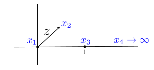
Figure 2: (Color online) Conformal frame defining the $z$ coordinate. Figure from Hogervorst and Rychkov (2013).

For 4 points, we can first find a conformal transformation fixing 3 of them as above, and then rotate around the axis to put the fourth point into a fixed plane (we assume that $d\geqslant 2$). The resulting configuration can be parametrized in Euclidean signature as ($\mathbf{0}\equiv\mathbf{0}_{d-2}$)

$$x_{1} =(0,0,\mathbf{0})\,,\quad x_{2}=(\sigma,\tau,\mathbf{0})\,,$$

$$x_{3} =(1,0,\mathbf{0})\,,\quad x_{4}=(\infty,0,\mathbf{0})\,.$$ (29)

It is customary to define (see Fig. 2)

$$z=\sigma+i\tau,\quad\bar{z}=\sigma-i\tau\,,$$ (30)

which are complex conjugate variables if we are working in the Euclidean. The conformal cross ratios can be expressed in terms of $z$, $\bar{z}$ as

$$u=z\bar{z}\,,\qquad v=(1-z)(1-\bar{z})\,.$$ (31)

A choice of points $x_{i}$, as in Eq. (29), is called a conformal frame. It can be thought of as a gauge fixing of most or all of the conformal symmetry. By construction, any coordinate configuration can be reduced to the conformal frame form. Therefore, the knowledge of a correlation function in the conformal frame is sufficient to reconstruct it at any other point through its covariance properties Osborn and Petkou (1994). The functional forms of 2pt and 3pt functions are fixed because their conformal frames do not contain any free parameters. The 4pt conformal frame (29) has 2 real parameters, explaining the functional freedom of the conformal 4pt function. See Sec. III.6.2 for another frequently used conformal frame.

Conformal frames provide a way to construct conformal correlators which is sometimes more convenient than the embedding formalism described in App. A. This method can also be used to classify the allowed tensor structures. An important role is then played by the stabilizer group, defined as the set of conformal transformations leaving the conformal frame configuration invariant. It is $SO(d-1)$ for 3pt functions and $SO(d-2)$ for 4pt functions. One classifies tensor structures invariant under the stabilizer group, and each of them lifts to an independent conformally invariant tensor structure Kravchuk and Simmons-Duffin (2018a). This method is particularly useful when dealing with 4pt functions of tensor operators: it does not overcount tensor structures, which may happen in the embedding formalism unless special care is taken.

III.4 Operator product expansion

Our point of view on the origin and the role of the Operator Product Expansion (OPE) in CFT is the one pedagogically reviewed in Rychkov (2016b); Simmons-Duffin (2017b). Here we will present the main logic and set some conventions.

The key idea is that of radial quantization, which says that we can represent Euclidean CFT correlation functions as scalar products of states $\langle\Psi_{\rm out}|\Psi_{\rm in}\rangle$ which live on a sphere of radius $R$. The state $|\Psi_{\rm in}\rangle$ is generated by operators in the interior of the sphere, while $\langle\Psi_{\rm out}|$ by those in the exterior. Once we replace the interior operators by the state $|\Psi_{\rm in}\rangle$, in a scale invariant theory we can scale the radius of the sphere to zero. Thus any state $|\Psi_{\rm in}\rangle$ can be expanded in a basis of local operators inserted at the center of the sphere. This is called the state-operator correspondence.

The OPE, written schematically in (5), is just the special case of the above when there are two operators at points $x_{1}$ and $x_{2}$ inside the sphere centered at $y$. We also see the origin of the OPE convergence criterion (7), since we need to have a separating sphere to start the argument.

As discussed in Sec. II, the next step is to group primaries and descendants in the OPE and to impose the constraints of conformal invariance. This gives the “conformal OPE”:

$${\cal O}_{\Delta_{i}}(x_{1}){\cal O}_{\Delta_{j}}(x_{2})=\sum_{k}\lambda_{ijk}\hat{f}_{ijk}(x_{1},x_{2},y,\partial_{y}){\cal O}_{\Delta_{k}}(y)\,.$$ (32)

The differential operator $\hat{f}_{ijk}$ is fixed by conformal invariance. It can be determined by demanding that the conformal OPE reproduce the 3pt function $\langle{\cal O}_{\Delta_{i}}(x_{1}){\cal O}_{\Delta_{j}}(x_{2}){\cal O}_{\Delta_{k}}^{\dagger}(x_{3})\rangle$, whose form is by itself fixed by conformal invariance up to the constants $\lambda_{ijk}$.

Any $SO(d)$ (or $Spin(d)$) index which the operators ${\cal O}_{\Delta_{i}}$ may have are left implicit in (32). Depending on their representations, there may be several allowed 3pt function tensor structures, and then each structure comes with its own OPE coefficient and a corresponding conformally-invariant differential operator $\hat{f}_{ijk}$. In the most frequently occurring case where ${\cal O}_{\Delta_{i}}$ and ${\cal O}_{\Delta_{j}}$ are scalars and ${\cal O}_{\Delta_{k},\ell}$ a spin-$\ell$ traceless symmetric tensor there is just one OPE coefficient.

While it is important to know that the conformal OPE exists and converges, it turns out that in practice one rarely needs its full explicit form. For example, conformal block computations can be organized in ways which avoid explicit knowledge of the full OPE, see Sec. III.6. For this reason, one frequently writes only the “leading OPE”, i.e. the primary term.

For example, in the above-mentioned case of two scalars and a traceless symmetric tensor, the leading OPE has the form (specializing to $x_{1}=x$, $x_{2}=y=0$):

$${\cal O}_{\Delta_{i}}(x){\cal O}_{\Delta_{j}}(0)\supset\lambda_{ijk}\frac{x_{\mu_{1}}\cdots x_{\mu_{\ell}}}{(x^{2})^{(h_{ijk}+\ell)/2}}{\cal O}^{\mu_{1}\ldots\mu_{\ell}}_{\Delta_{k},\ell}(0)+\ldots\,.$$ (33)

This reproduces the leading asymptotics of the 3pt function (23) in the limit $x\to 0$ with $x_{3}$ fixed, including the normalization, provided that the 2pt function of ${\cal O}_{\Delta_{k},\ell}$ is unit-normalized as in (22). Occasionally we will schematically write such a leading OPE as ${\cal O}_{\Delta_{i}}\times{\cal O}_{\Delta_{j}}\supset{\cal O}_{\Delta_{k},\ell}$, but the form (33) should always be understood.

As explained in Sec. II, any $n$-point function can be computed from the CFT data by repeated application of the OPE. The 4pt function case, of primary importance for the bootstrap, will be discussed in Sec. III.6.

III.5 Constraints from unitarity

Here we will review the notion of a unitary CFT, focusing on the constraints on CFT data arising for such theories which make the bootstrap especially powerful.

Unitary CFTs can be considered both in Lorentzian and Euclidean signature. They are characterized in the latter by a property called reflection positivity. On the other hand, nonunitary CFTs are generally expected to make sense only in Euclidean signature. They will be discussed briefly in Sec. VIII.

Unitary theories allow for quantization in a Hilbert space with a positive-definite norm. In the quantization by planes normally used in Euclidean QFT, an “in” state $|\Psi\rangle$ is generated by $n$ local operators ${\cal O}_{i}$ inserted in the half-space $x_{1}<0$, and an “out” state $\langle\Psi|$ is generated by reflected operators ${\cal O}_{i}^{\dagger}$, inserted at $x_{1}>0$ at mirror-symmetric positions. Unitarity implies that the norm $\langle\Psi|\Psi\rangle$ must be non-negative. This norm is just a $2n$-point function in a particular kinematic configuration, and its positivity is called (Osterwalder-Schrader) reflection positivity.

Analogously, in the radial quantization usually used for CFTs, an “in” state $|\Psi\rangle$ is generated by local operators ${\cal O}_{i}$ inserted at positions $x_{i}$ inside the unit sphere $(i=1,\ldots,n)$, and a conjugate “out” state $\langle\Psi|$ is generated by operators ${\cal O}_{i}^{\dagger}$ inserted at positions related by an inversion transformation $x_{i}^{\prime}=x_{i}/x^{2}$. The norm $\langle\Psi|\Psi\rangle$, which is just an inversion-symmetric $2n$-point function, must be non-negative, a property we will call “inversion positivity”. In CFTs, both forms of positivity are equivalent, and they are both useful depending on circumstances.

III.5.1 Unitarity bounds

We already get a simple and powerful constraint by considering radial quantization states $|\Psi\rangle$ produced by a local operator ${\cal O}$ acting at the origin. In this case the conjugate operator is inserted at infinity. For a primary ${\cal O}$ we recover that its 2pt function must have positive normalization and hence can be normalized to one as in (22). Additional constraints arise from considering descendants of ${\cal O}$. The conformal algebra computes the norms of descendants as polynomials in the primary dimension $\Delta$. Imposing that all descendants have a non-negative norm gives a lower bound on $\Delta$. This “unitarity bound” depends on the representation $r$ of $SO(d)$ (or its double cover for spinor representations) in which the primary transforms.

In 3d, the representation $r$ is labeled by a half-integer $j$, with $j=\ell$ for traceless symmetric spin-$\ell$ tensors. The unitarity bounds are

$$d=3:\quad \Delta\geqslant 1/2 (\text{scalar, }j=0)\,,$$

$$\Delta\geqslant 1 (\text{smallest spinor, }j=1/2)\,,$$ (34)

$$\Delta\geqslant j+1\ (j>1/2)\,.$$

In 4d, we can label the representation $r$ by two integers $(\ell,\bar{\ell})$, with traceless symmetric spin-$\ell$ tensors having $\ell=\bar{\ell}$. The unitarity bounds then read

$$d=4:\quad \Delta\geqslant 1 (\text{scalar, }\ell=\bar{\ell}=0)\,,$$

$$\Delta\geqslant{\textstyle\frac{1}{2}}\ell+1 (\ell>0,\bar{\ell}=0)\,,$$ (35)

$$\Delta\geqslant{\textstyle\frac{1}{2}}(\ell+\bar{\ell})+2 (\ell\bar{\ell}\neq 0)\,.$$

For the 5d and 6d unitarity bounds see Minwalla (1998). For some representations occurring in all dimensions the unitarity bounds can be written in dimension-independent form as follows:

$$\Delta\geqslant{\textstyle\frac{1}{2}}(d-2) (\text{scalar})\,,$$

$$\Delta\geqslant{\textstyle\frac{1}{2}}(d-1) (\text{smallest spinor})\,,$$ (36)

$$\Delta\geqslant\ell+d-2 (\text{traceless symmetric, spin }\ell\geqslant 1)\,.$$

As a final comment, in physics literature the unitarity bounds are often derived by imposing positivity of the descendant norms on the first (and the second, for scalars) level. It is a nontrivial fact that no further constraints arise from higher levels. See Bourget and Troost (2018, Tables 3 and 5) for a review of rigorous mathematical results for unitary bounds in any $d$.

III.5.2 OPE coefficients

Unitarity also gives reality constraints on OPE coefficients of real operators. Consider the 3pt function (23) between two scalars and a traceless symmetric tensor, assuming all three operators are real. Then the 3pt function coefficient must be real:

$$\lambda_{123}\in\mathbb{R}\,.$$ (37)

To argue this, we can consider a 6pt function $\langle{\cal O}_{1}{\cal O}_{2}(\Theta{\cal O}_{3}){\cal O}_{3}{\cal O}_{2}{\cal O}_{1}\rangle$, with the operators arranged mirror-symmetrically against a plane into two compact groups positioned a large distance from each other (see Fig. 3). Here $\Theta$ is the reflection factor mentioned in footnote 39. Reflection positivity implies that this 6pt function should be real and positive. On the other hand, by cluster decomposition this 6pt function is equal to the product of two distant 3pt functions, which is easily seen to be $\lambda_{123}^{2}$ times a positive number. So (37) follows. We stress that this conclusion holds for both even and odd $\ell$.

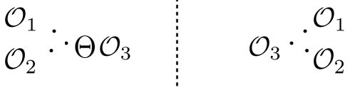
Figure 3: Positivity of this 6pt function implies reality of the 3pt function coefficient $\lambda_{123}$, see the text.

It was important for the above argument that the tensor structure entering (23) was parity invariant (i.e., it did not involve the $\epsilon$-tensor). This argument can be generalized to OPE coefficients for general 3pt tensor structures. The OPE coefficients of tensor structures must be purely imaginary or real depending on whether they involve the $\epsilon$-tensor or not. One must similarly be careful with OPE coefficients involving spinors.

Consider now the 4pt function $\langle{\cal O}_{2}{\cal O}_{1}{\cal O}_{1}{\cal O}_{2}\rangle$ where ${\cal O}_{1}$ and ${\cal O}_{2}$ are real scalars and the point configuration is reflection-symmetric or inversion-symmetric. This 4pt function should be non-negative as a basic consequence of unitarity, and Eq. (37) implies that a more nuanced statement is true: the individual contribution of every primary ${\cal O}$ to this 4pt function is non-negative, see Eq. (43) below. This can be generalized to external operators in general $SO(d)$ (or $Spin(d)$) representations, including the case when there are multiple 3pt function tensor structures.

To summarize, the unitarity bounds say that the CFT Hilbert space has a positive-definite norm, and the OPE coefficient reality constraints say that the OPE preserves this positive-definite structure. If the CFT data satisfies both of these constraints, we are guaranteed that the CFT will be unitary. The bootstrap obtains further constraints on CFT data by combining unitarity with crossing relations.

III.5.3 Averaged null energy condition

In a QFT in Lorentzian signature, we can consider the integral of the stress tensor component $T_{++}$ along a light ray: the light-like direction $x^{+}$ with all other coordinates fixed to zero. The averaged null energy condition (ANEC) says that this light-ray operator has a non-negative expectation value in any state:

$$\langle\Phi|\int_{-\infty}^{\infty}dx^{+}\,T_{++}|\Phi\rangle\geqslant 0\,.$$ (38)

The ANEC should hold in any unitary QFT. Two general proofs of the ANEC were given recently, one via quantum information Faulkner et al. (2016), and one by causality Hartman et al. (2017). Specializing to CFTs, the causality argument makes it clear that the ANEC is not an extra assumption but follows from other CFT axioms such as unitarity, the OPE, and crossing relations for correlation functions involving $T_{\mu\nu}$. Notice however that any results following from the ANEC will require the existence of a local stress-tensor operator.

Choosing $|\Phi\rangle$ in (38) to be generated by a local operator ${\cal O}$ acting on the vacuum, the ANEC leads to positivity constraints on 3pt functions $\langle{\cal O}T_{\mu\nu}{\cal O}\rangle$ called “conformal collider bounds” Hofman and Maldacena (2008).

Recently, Cordova and Diab (2018) used the ANEC to argue that primaries of high chirality (large $|\ell-\bar{\ell}|$) in unitary 4d CFTs should satisfy unitarity bounds stronger than (35). From partial checks for $\bar{\ell}=0,1$, they conjecture the general bound (assuming $\ell\geqslant\bar{\ell}$)

$$\Delta\geqslant\ell\,.$$ (39)

If $\bar{\ell}=0$ this becomes stronger than (35) for $\ell>2$ and for $\ell>\bar{\ell}+4$ otherwise. This can be viewed as a CFT strengthening of the theorem of Weinberg and Witten (1980).

III.6 Conformal blocks

Conformal blocks are of capital importance for the bootstrap. Their theory was initiated in 1970s Ferrara et al. (1972, 1974b, 1975), with further advances in the early 2000s Dolan and Osborn (2001a, 2004) which were crucial for the bootstrap revival. Recently it experienced further rapid developments, and here we will review its current state.

Consider a 4pt function of four primary scalar operators $\phi_{i}(x_{i})$ with $i=1,\ldots,4$ (see Sec. III.6.7 for the general case of external operators with spin). As mentioned in Sec. II, this 4pt function can be computed by applying the OPE of Eq. (5) to two pairs of fields. For definiteness we fix here the pairing $\phi_{1}(x_{1})\phi_{2}(x_{2})$ and $\phi_{3}(x_{3})\phi_{4}(x_{4})$. This is referred to as “the (12)-(34) OPE channel”, to distinguish it from other pairings which will play a role when we discuss crossing. This gives an expansion

$$\langle\phi_{1}(x_{1})\phi_{2}(x_{2})\phi_{3}(x_{3})\phi_{4}(x_{4})\rangle=\sum_{\cal O}\lambda_{12{\cal O}}\lambda_{34{\cal O}}\,{\rm W}_{\cal O}\,,$$ (40)

where ${\rm W}_{\cal O}\equiv{\rm W}_{\cal O}(x_{i})$ are the conformal partial waves (CPWs) given by

$${\rm W}_{\cal O}=\hat{f}_{12{\cal O}}(x_{1},x_{2},y,\partial_{y})\hat{f}_{34{\cal O}}(x_{3},x_{4},y^{\prime},\partial_{y^{\prime}})\langle{\cal O}(y){\cal O}(y^{\prime})\rangle\,.$$ (41)

Since the 2pt function is diagonal, the summation is over the same operator ${\cal O}$ in both OPEs. It follows from conformal invariance of the OPE that each CPW transforms under the conformal transformations in the same way as the 4pt function itself, see e.g. Costa et al. (2011a). It is then conventional to split off the factor ${\bf K}_{4}$ defined in Eq. (27), so that we finally have

$${\rm W}_{{\cal O}}=g^{\Delta_{12},\Delta_{34}}_{\Delta_{\cal O},\ell_{\cal O}}(u,v)\,{\bf K}_{4}\,,$$ (42)

where $g^{\Delta_{12},\Delta_{34}}_{\Delta_{\cal O},\ell_{\cal O}}(u,v)$ is called the conformal block. It represents the contribution of a primary ${\cal O}$ and all of its descendants to the 4pt function. As shown, it depends on the dimension and spin of the exchanged traceless symmetric primary ${\cal O}$, and also on the dimension differences $\Delta_{12}$, $\Delta_{34}$ of the external scalars. Comparing with Eq. (26), we thus have:

$$g(u,v)=\sum_{\cal O}\lambda_{12{\cal O}}\lambda_{34{\cal O}}\,g^{\Delta_{12},\Delta_{34}}_{\Delta_{\cal O},\ell_{\cal O}}(u,v)\,.$$ (43)

Eqs. (40) and (43) are referred to as the CPW decomposition and the conformal block decomposition.

Let us briefly discuss the regions of convergence of the considered expansions. If one works in the $z$ conformal frame of Eq. (29) in Euclidean signature, then Eq. (41) defining the CPWs converges for $|z|<1$, and the conformal block decomposition (43) is also seen to converge in this region, at least if the theory is unitary Pappadopulo et al. (2012). While this is sufficient for many applications, a stronger convergence result can be established using the $\rho$ frame, see Sec. III.6.2 below.

The above definition of conformal blocks via the conformal OPE is important in principle. In practice, there exist efficient approaches to compute the blocks which avoid needing explicit knowledge of the conformal OPE. They will be described below.

III.6.1 The Casimir equation

Let us consider the following alternative representation of CPWs. In radial quantization, as mentioned in Sec. III.4, the above 4pt function is expressed as a scalar product of two states

$$\langle\phi_{3}(x_{3})\phi_{4}(x_{4})|\phi_{1}(x_{1})\phi_{2}(x_{2})\rangle\,$$ (44)

living on a sphere separating $x_{1},x_{2}$ from $x_{3},x_{4}$. The CPW then corresponds to inserting an orthogonal projector ${\cal P}_{\Delta,\ell}$ onto the conformal multiplet of ${\cal O}_{\Delta,\ell}$:

$$\lambda_{12{\cal O}}\lambda_{34{\cal O}}\,{\rm W}_{\cal O}=\langle\phi_{3}(x_{3})\phi_{4}(x_{4})|{\cal P}_{\Delta,\ell}|\phi_{1}(x_{1})\phi_{2}(x_{2})\rangle\,.$$ (45)

For future reference, the projector can be written as

$${\cal P}_{\Delta,\ell}=\sum_{\alpha,\beta={\cal O},P{\cal O},PP{\cal O},\ldots}|\alpha\rangle G^{\alpha\beta}\langle\beta|\,,$$ (46)

where $G_{\alpha\beta}=\langle\alpha|\beta\rangle$ is the Gram matrix of the multiplet and $G^{\alpha\beta}$ is its inverse.

Furthermore, consider the quadratic Casimir

$$\mathcal{C}_{2}=\frac{1}{2}{\cal J}_{AB}{\cal J}^{BA}\,,$$ (47)

where ${\cal J}_{AB}$ are the $SO(d+1,1)$ generators, Eq. (14). Insert this operator into Eq. (45) right after ${\cal P}_{\Delta,\ell}$. The resulting expression can be computed in two ways. When we act with $\mathcal{C}_{2}$ on the left we have

$${\cal P}_{\Delta,\ell}\,{\mathcal{C}}_{2}=C_{\Delta,\ell}{\cal P}_{\Delta,\ell}\,,$$ (48)

where $C_{\Delta,\ell}$ is the quadratic Casimir eigenvalue:

$$C_{\Delta,\ell}=\Delta(\Delta-d)+\ell(\ell+d-2)\,.$$ (49)

On the other hand, the action of $\mathcal{C}_{2}$ on the right can be computed using the representation of the conformal generators on primaries as first-order differential operators, mentioned in Sec. III.2. We conclude that the CPW, and hence the conformal block, satisfies a second-order partial differential equation. The actual form of this “Casimir equation” is most conveniently found using the embedding formalism Dolan and Osborn (2004). In the $z,\bar{z}$ coordinates of Eq. (31) it takes the form

$$\mathcal{D}\,g^{\Delta_{12},\Delta_{34}}_{\Delta,\ell}(z,\bar{z})=C_{\Delta,\ell}\,\,g^{\Delta_{12},\Delta_{34}}_{\Delta,\ell}(z,\bar{z})\,,$$ (50)

where

$$\mathcal{D}=\mathcal{D}_{z}+\mathcal{D}_{\bar{z}}+2(d-2)\frac{z\bar{z}}{z-\bar{z}}[(1-z)\partial_{z}-(1-\bar{z})\partial_{\bar{z}}]\,,$$

$$\mathcal{D}_{z}=\textstyle 2z^{2}(1-z)\partial_{z}^{2}-(2+\Delta_{34}-\Delta_{12})z^{2}\partial_{z}+\frac{\Delta_{12}\Delta_{34}}{2}z\,.$$ (51)

Moreover, the leading $z,\bar{z}\to 0$ behavior of the conformal block can be easily determined using the OPE, and this provides boundary conditions for Eq. (50). Considering the $x_{12},x_{34}\rightarrow 0$ limit in Eq. (42) and using Eqs. (22) and (33), one obtains

$$g^{\Delta_{12},\Delta_{34}}_{\Delta,\ell}(z,\bar{z})\underset{z,\bar{z}\rightarrow 0}{\sim}{\cal N}_{d,\ell}\,(z\bar{z})^{\frac{\Delta}{2}}{\rm Geg}_{\ell}\left(\frac{z+\bar{z}}{2\sqrt{z\bar{z}}}\right)\,,$$ (52)

where ${\rm Geg}_{\ell}(x)$ is a Gegenbauer polynomial,

$${\rm Geg}_{\ell}(x)=C^{(d/2-1)}_{\ell}(x)\,,$$ (53)

and the normalization factor ${\cal N}_{d,\ell}$ is given by

$${\cal N}_{d,\ell}=\frac{\ell!}{{(-2)^{\ell}}(d/2-1)_{\ell}}\,.$$ (54)

We warn the reader that many different normalization choices can be found in the literature. Different conformal block normalizations correspond to different normalizations of OPE coefficients as compared with the one in Eq. (33). In this review we will use the above normalization unless mentioned otherwise. For the reader’s convenience, we have collected some other frequently used normalizations in Table 1.

${\cal N}_{d,\ell}$	Reference
$\frac{\ell!}{(-2)^{\ell}(d/2-1)_{\ell}}$	Dolan and Osborn (2001b, 2004), Rattazzi et al. (2008), Penedones et al. (2016), this review
$\frac{\ell!}{(d-2)_{\ell}}$	Dolan and Osborn (2011), Hogervorst and Rychkov (2013), El-Showk et al. (2012, 2014b), Costa et al. (2016b), JuliBoots Paulos (2014b), cboot Ohtsuki (2016)
$\frac{(-1)^{\ell}\ell!}{4^{\Delta}(d/2-1)_{\ell}}$	Kos et al. (2014a, 2015b, 2016), Li et al. (2017b) PyCFTBoot Behan (2017a)
$\frac{\ell!}{(d/2-1)_{\ell}}$	Poland et al. (2012), Poland and Stergiou (2015)
$\frac{\ell!}{4^{\Delta}(d-2)_{\ell}}$	Kos et al. (2014b) Mathematica notebook Simmons-Duffin (2015b)
$\frac{(-1)^{\ell}\ell!}{(d/2-1)_{\ell}}$	Simmons-Duffin (2017c)

Table 1: Summary of various conformal block normalizations ${\cal N}_{d,\ell}$, Eqs. (52, 62), used in the literature.

By solving Eq. (50) one can find conformal blocks for even $d$ Dolan and Osborn (2004). They are expressed in terms of the basic function

$$k_{\beta}(x)=x^{\beta/2}{}_{2}F_{1}\left(\frac{\beta-\Delta_{12}}{2},\frac{\beta+\Delta_{34}}{2},\beta;x\right)\,,$$ (55)

which satisfies

$$\mathcal{D}_{x}k_{\beta}(x)=\frac{1}{2}\beta(\beta-2)k_{\beta}(x)\,,\quad k_{\beta}(x)\underset{x\rightarrow 0}{\sim}x^{\beta/2}\,.$$ (56)

In the simplest case of $d=2$, we have ${\cal D}={\cal D}_{z}+{\cal D}_{\bar{z}}$, so the conformal blocks factorize. They take the form

$$d=2:\quad g^{\Delta_{12},\Delta_{34}}_{\Delta,\ell}(z,\bar{z})=\frac{1}{(-2)^{\ell}(1+\delta_{\ell 0})}\\ \times\left(k_{\Delta+\ell}(z)k_{\Delta-\ell}(\bar{z})+z\leftrightarrow\bar{z}\right)\,.$$ (57)

Results for higher even $d$ can then be found using recursion relations relating blocks in $d$ and $d+2$ dimensions Dolan and Osborn (2004). The important case of $d=4$ reads

$$d=4:\quad g^{\Delta_{12},\Delta_{34}}_{\Delta,\ell}(z,\bar{z})=\frac{1}{(-2)^{\ell}}\\ \times\frac{z\bar{z}}{z-\bar{z}}\left(k_{\Delta+\ell}(z)k_{\Delta-\ell-2}(\bar{z})-z\leftrightarrow\bar{z}\right)\,.$$ (58)

In odd $d$, general closed-form solutions of the Casimir equation are so far unavailable. Sometimes, one can get closed-form solutions along the “diagonal” $z=\bar{z}$, as e.g. in $d=3$ for all equal external dimensions (Rychkov and Yvernay, 2016, Eqs. (3.7-3.10)). Other expressions along the diagonal, valid for any $d$, can be found in Hogervorst et al. (2013). Using these results as a starting point, one can compute derivatives of conformal blocks orthogonal to the diagonal using the Casimir equation, by the Cauchy-Kovalevskaya method, see Sec. III.6.5. The knowledge of these derivatives is usually sufficient for numerical conformal bootstrap applications. Other techniques used to access the conformal blocks numerically will be discussed below.

Finally, let us mention that conformal blocks have simple transformation properties under the interchange of external operators $1\leftrightarrow 2$ and $3\leftrightarrow 4$ Dolan and Osborn (2001b, 2011):

$$g^{\Delta_{12},\Delta_{34}}_{\Delta,\ell}(u/v,1/v)=(-1)^{\ell}v^{\frac{\Delta_{34}}{2}}g^{-\Delta_{12},\Delta_{34}}_{\Delta,\ell}(u,v)$$

$$\hskip 85.35826pt=(-1)^{\ell}v^{-\frac{\Delta_{12}}{2}}g^{\Delta_{12},-\Delta_{34}}_{\Delta,\ell}(u,v)\,.$$ (59)

This follows from the symmetry of the OPE under the same interchange. As a check, the explicit expressions in Eqs. (57-58) satisfy these relations.

III.6.2 Radial expansion for conformal blocks

While closed-form expressions for conformal blocks in general $d$ are unknown, there exist rapidly convergent power series expansions. Following Hogervorst and Rychkov (2013), we will describe a particular conformal frame used to generate such expansions.

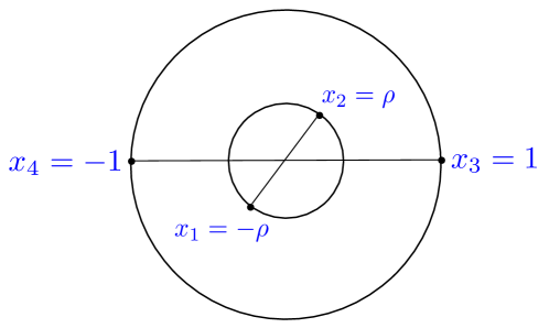
Figure 4: (Color online) Conformal frame defining the radial coordinate. Figure from Hogervorst and Rychkov (2013).

Starting from the conformal frame (29), we apply an additional conformal transformation which keeps the four points in the same 2-plane but moves them into a configuration symmetric around the origin as in Fig. 4. So the points $x_{1}=-x_{2}$ are now on a circle of radius $r<1$, while $x_{3}=-x_{4}$ lie on the unit circle.

Let us call ${\bf n}$ and $\bf{n}^{\prime}$ the unit vectors pointing to $x_{2}$ and $x_{3}$, and introduce the complex radial coordinate Pappadopulo et al. (2012)

$$\rho=re^{i\theta}\,,\qquad{\bf n}\cdot{\bf n}^{\prime}=\cos\theta=\eta\,,$$ (60)

which is related to the variable $z$ in Eq. (30) via

$$\rho=\frac{z}{(1-\sqrt{1-z})^{2}}\,,\qquad z=\frac{4\rho}{(1+\rho)^{2}}\,.$$

See Hogervorst and Rychkov (2013) for why $\rho$ is preferable to $z$ for constructing rapidly convergent power series expansions for conformal blocks.

In this configuration, the 4pt function is interpreted as a matrix element between two radial quantization states: $\langle\phi_{3}(1,{\bf n}^{\prime})\phi_{4}(1,-{\bf n}^{\prime})|$ and $|\phi_{1}(r,-{\bf n})\phi_{2}(r,{\bf n})\rangle=r^{D}|\phi_{1}(1,-{\bf n})\phi_{2}(1,{\bf n})\rangle$. The factor $r^{D}$, with $D$ the dilatation generator, takes care of the radial dependence.

Consider then the conformal partial wave given in Eq. (45). The conformal multiplet of the operator ${\cal O}_{\Delta,\ell}$ at level $m$ contains descendants $|\Delta+m,j\rangle$ of spin $j$ varying from $\max(0,\ell-m)$ to $\ell+m$. We need to know the matrix elements between these descendants and the above in and out states. Leaving aside the overall normalization of these matrix elements, their dependence on the unit vector $\mathbf{n}$ must be proportional to the traceless symmetric tensor $({\bf n}_{\mu_{1}}\ldots{\bf n}_{\mu_{j}}-\text{traces})$. Contracting two such tensors for $\mathbf{n}$ and $\mathbf{n}^{\prime}$ gives, up to a constant factor, the Gegenbauer polynomial ${\rm Geg}_{j}({\bf n}\cdot{\bf n^{\prime}})$ from Eq. (53).

We conclude that the conformal block has a power series expansion of the form

$$g^{\Delta_{12},\Delta_{34}}_{\Delta,\ell}(u,v)=r^{\Delta}\sum_{m=0}^{\infty}r^{m}\sum_{j}w(m,j)\;{\rm Geg}_{j}(\eta)\,,$$ (61)

where $w(m,j)\neq 0$ only for $\max(0,\ell-m)\leqslant j\leqslant\ell+m$. Using unitarity, one can also conclude that $w(m,j)\geqslant 0$ if $\Delta$ is above the unitarity bound and $\Delta_{12}=-\Delta_{34}$.

Since $z\sim 4\rho$ at small $z$, the OPE limit (52) becomes

$$g^{\Delta_{12},\Delta_{34}}_{\Delta,\ell}(r,\eta)\displaystyle\underset{r\rightarrow 0}{\sim}{\cal N}_{d,\ell}(4r)^{\Delta}{\rm Geg}_{\ell}\left(\eta\right)\,,$$ (62)

which fixes $w(0,\ell)={\cal N}_{d,\ell}4^{\Delta}$. To find higher $w(m,j)$, one must determine the normalization of the descendant matrix elements and not just their dependence on $\mathbf{n},\mathbf{n}^{\prime}$. While in principle this can be done using conformal algebra, two more efficient techniques will be discussed below.

The expansion (61) converges for $|\rho|<1$, showing that conformal blocks are smooth and real-analytic functions in this region. The conformal block decomposition (43) can be similarly argued to converge for $|\rho|<1$. In terms of the $z$ coordinate, this covers the whole complex plane minus the cut $(1,+\infty)$, improving the convergence result argued below Eq. (43) using the $z$ frame.

III.6.3 Recursion relation from the Casimir equation

The first method to find the coefficients $w(m,j)$ is to substitute the expansion (61) into the Casimir equation. This gives rise to recurrence relations, obtained in Hogervorst and Rychkov (2013) and Costa et al. (2016b), which determine $w(m,j)$ for $m>0$ starting from $w(0,\ell)$.

Namely, defining the functions $f_{m,j}\equiv r^{m}{\rm Geg}_{j}(\eta)$, it is straightforward to show that any of the operators $\{r,\eta,\partial_{r},\partial_{\eta}\}$ acting on these functions produces linear combinations of $f_{m\pm 1,j\pm 1}$. Similarly, the operator ${\cal D}$ in (50), when written in radial coordinates, maps $f_{m,j}$ into a linear combination of $f_{m+\hat{m},j+\hat{\jmath}}$ functions with suitable shifts. Eq. (50) then gives rise to a relation which can be economically written in the form Costa et al. (2016b)

$$\sum_{(\hat{m},\hat{\jmath})\in\mathcal{S}}c(\hat{m},\hat{\jmath})\;w(m+\hat{m},j+\hat{\jmath})=0\ ,$$ (63)

where the set $\mathcal{S}=\{(0,0),(-1,1),(-1,-1),\ldots\}$ contains $30$ points, all of which but the first have $\hat{m}<0$. The coefficients $c(\hat{m},\hat{\jmath})$ are known functions of the variables $\Delta_{12}$, $\Delta_{34}$, $\Delta$, $\ell$, $d$, $m$, and $j$ (Costa et al., 2016b, attached Mathematica notebook). Using Eq. (63), the coefficient $w(m,j)$ can then be recursively expressed in terms of $w(m^{\prime},j)$ with $m^{\prime}<m$.

III.6.4 Recursion relation from analytic structure

The second method exploits the analytic structure in $\Delta$ to obtain a recursion relation for the conformal blocks. A similar approach was first applied by Zamolodchikov (1984, 1987) to the 2d Virasoro conformal blocks, by considering them as meromorphic functions of the central charge $c$ or of the scaling dimension $\Delta$. For conformal blocks of external scalars in arbitrary $d$, this idea was introduced in Kos et al. (2014b, a). It was formalized and extended to conformal blocks for external operators with spin in Penedones et al. (2016). Here we will explain the external scalar case.

Eqs. (45), (46) provide a convenient starting point for discussing the analytic structure of a conformal block as a function of the exchanged primary dimension $\Delta$. When $\Delta$ is above the unitarity bound, the Gram matrix $G_{\alpha\beta}(\Delta)$ is positive-definite and invertible. However it turns out that for special values of $\Delta=\Delta_{A}^{*}$ at or below the unitarity bounds, the Gram matrix becomes degenerate, in the sense that some states are null (i.e. have zero norm). The conformal block then develops a pole in $\Delta-\Delta^{*}_{A}$. Here we will assume that there are only simple poles, as is true for example in odd $d$, while for even $d$ simple poles coalesce into double ones, see below.

The crucial observation is that the residue of the pole is proportional to another conformal block:

$$g^{\Delta_{12},\Delta_{34}}_{\Delta,\ell}(r,\eta)\sim\frac{R_{A}}{\Delta-\Delta^{*}_{A}}g^{\Delta_{12},\Delta_{34}}_{\Delta_{A},\ell_{A}}(r,\eta)\,.$$ (64)

Namely, we identify the first descendant state ${\cal O}_{A}^{\rm null}$ of ${\cal O}$ which becomes null when $\Delta\to\Delta_{A}^{*}$. Let $\Delta_{A}=\Delta_{A}^{*}+n_{A}$ be its dimension in this limit, and $\ell_{A}$ its spin. It can be shown that ${\cal O}_{A}^{\rm null}$ is annihilated by $K_{\mu}$ when $\Delta\to\Delta_{A}^{*}$ and so can be thought of as both a descendant and a primary. Consider then a fictitious primary ${\cal O}_{A}$ which has quantum numbers $(\Delta_{A},\ell_{A})$ and which is unit-normalized. It is the conformal block of such a primary, with standard normalization (62), that appears in the residue.

To be more precise, consider the rate with which ${\cal O}_{A}^{\rm null}$ becomes null as $\Delta\to\Delta_{A}^{*}$:

$$\langle{\cal O}_{A}^{\rm null}|{\cal O}_{A}^{\rm null}\rangle\sim Q_{A}(\Delta-\Delta_{A}^{*})\,,$$ (65)

with $Q_{A}$ some constant. When ${\cal O}_{A}^{\rm null}$ becomes null, all of its descendants become null too, with the rate proportional to (65). Moreover, it can be shown that the Gram matrix in the submultiplet consisting of these descendants is equal to (65) times the (non-singular) Gram matrix of the multiplet of ${\cal O}_{A}$, up to corrections of higher order in $\Delta-\Delta_{A}^{*}$. This explains why the residue in (64) involves the whole conformal block of ${\cal O}_{A}$.

The coefficient $R_{A}$ in $(\ref{eq:resid})$ is a product of three factors:

$$R_{A}=M_{A}^{(L)}Q^{-1}_{A}M_{A}^{(R)}\ ,$$ (66)

where $Q_{A}$ is defined in (65), while $M_{A}^{(L)}$ and $M_{A}^{(R)}$ come from the 3pt functions $\langle\phi_{3}\phi_{4}|{\cal O}_{A}^{\rm null}\rangle$ and $\langle{\cal O}_{A}^{\rm null}|\phi_{1}\phi_{2}\rangle$.

Using information about the poles, we can now write a complete formula for the conformal block. It is convenient to define the regularized conformal block $h_{\Delta,\ell}\equiv h^{\Delta_{12},\Delta_{34}}_{\Delta,\ell}$ by removing a $(4r)^{\Delta}$ prefactor:

$$g^{\Delta_{12},\Delta_{34}}_{\Delta,\ell}(r,\eta)=(4r)^{\Delta}h_{\Delta,\ell}(r,\eta)\,.$$ (67)

The function $h_{\Delta,\ell}$ has the same poles in $\Delta$ as $g_{\Delta,\ell}$. Moreover it is a meromorphic function of $\Delta$, and is therefore fully characterized by its poles and the value at infinity:

$$h_{\Delta,\ell}(r,\eta)=h_{\infty,\ell}(r,\eta)\\ +\sum_{A}\frac{R_{A}}{\Delta-\Delta^{*}_{A}}(4r)^{n_{A}}\,h_{\Delta^{*}_{A}+n_{A},\ell_{A}}(r,\eta)\,.$$ (68)

Detailed analysis shows that the poles occurring in this equation organize into one finite and two infinite sequences:

$$\begin{array}[]{lccc}A&\Delta^{*}_{A}&n_{A}&\ell_{A}\\ \hline\cr\mbox{I${}_{n}$ }\ \ (n\in\hbox{$N$})&1-\ell-n&n&\ell+n\\ \mbox{II${}_{n}$ }\ (1\leqslant n\leqslant\ell)&\ell+d-1-n&n&\ell-n\\ \mbox{III${}_{n}$ }(n\in\hbox{$N$})&\frac{d}{2}-n&2n&\ell\\ \end{array}$$ (69)

Using this definition, it is easy to check that the residues of the poles themselves are nonsingular (except in even dimensions, see below).

The $h_{\infty,\ell}$ term and the constants $R_{A}$ are given by Kos et al. (2014a); Penedones et al. (2016)

$$h_{\infty,\ell}(r,\eta) =\textstyle\frac{\left(1-r^{2}\right)^{1-\frac{d}{2}}{\cal N}_{d,\ell}{\rm Geg}_{\ell}(\eta)}{\left(r^{2}-2\eta r+1\right)^{\frac{1-\Delta_{12}+\Delta_{34}}{2}}\left(r^{2}+2\eta r+1\right)^{\frac{1+\Delta_{12}-\Delta_{34}}{2}}}\,,$$

$$R_{\text{I}_{n}} =\textstyle\frac{-n(-2)^{n}}{(n!)^{2}}\left(\frac{\Delta_{12}+1-n}{2}\right)_{n}\left(\frac{\Delta_{34}+1-n}{2}\right)_{n}\ ,$$

$$R_{\text{II}_{n}} =\textstyle\frac{-n\,\ell!}{(-2)^{n}(n!)^{2}(\ell-n)!}\frac{(d+\ell-n-2)_{n}}{\left(\frac{d}{2}+\ell-n\right)_{n}\left(\frac{d}{2}+\ell-n-1\right)_{n}}$$ (70)

$$\quad\textstyle\times\left(\frac{\Delta_{12}+1-n}{2}\right)_{n}\left(\frac{\Delta_{34}+1-n}{2}\right)_{n}\ ,$$

$$R_{\text{III}_{n}} =\textstyle\frac{-n(-1)^{n}\left(\frac{d}{2}-n-1\right)_{2n}}{(n!)^{2}\left(\frac{d}{2}+\ell-n-1\right)_{2n}\left(\frac{d}{2}+\ell-n\right)_{2n}}$$

$$\quad\times\textstyle\left(\frac{\Delta_{12}-\frac{d}{2}-\ell-n+2}{2}\right)_{n}\left(\frac{\Delta_{12}+\frac{d}{2}+\ell-n}{2}\right)_{n}$$

$$\quad\times\textstyle\left(\frac{\Delta_{34}-\frac{d}{2}-\ell-n+2}{2}\right)_{n}\left(\frac{\Delta_{34}+\frac{d}{2}+\ell-n}{2}\right)_{n}\ .$$

The key property of Eq. (68) is that each pole residue comes with a factor $r^{n_{A}}$. This means that it can be used as a recursion relation to generate the regularized conformal block as a power series in $r$. Indeed, suppose we want to compute $h_{\Delta,l}(r,\eta)$ up to $O(r^{N})$. We use Eq. (68) keeping all poles with $n_{A}\leqslant N$, of which there are finitely many. The residues of these poles themselves are needed up to smaller order $O(r^{N-n_{A}})$, so we get a recursion relation. This is one of the most elegant and efficient currently known methods to compute the conformal blocks outside of even $d$.

The described recursion relation is adequate for computing conformal blocks in odd dimensions and also in generic $d$. It cannot be applied directly in even $d$, since some simple poles coalesce into double poles. This is not a problem, since even $d$ conformal blocks are known in closed form. Alternatively, one can apply the recursion relation $\epsilon$ away from an even $d$, and take the limit $\epsilon\to 0$ after the coefficients of the $r$ expansion have been generated. This gives the correct result because the conformal blocks vary analytically with $d$.

III.6.5 Rational approximation of conformal blocks and their derivatives

We will now describe how to construct rational approximations to conformal blocks and their derivatives at a given point $(r_{*},\eta_{*})$, which permit an efficient numerical evaluation of these quantities as a function of $\Delta$. This will play an important role in the numerical techniques described in Sec. IV. Our focus will be on rational approximations to scalar conformal blocks, but later in Sec. III.6.7 we will also describe how they can be extended to blocks for external spinning operators.

A rational approximation for conformal block derivatives at a given point can be obtained by combining the radial expansion (61) and the recursion relation (68). It can be expressed in the form

$$\partial_{r}^{m}\partial_{\eta}^{n}g_{\Delta,\ell}(r_{*},\eta_{*})=(4r_{*})^{\Delta}\left(\frac{P_{N}^{mn}(\Delta)}{Q_{N}(\Delta)}+O(r_{*}^{N-m})\right)\,.$$ (71)

Here $Q_{N}$ is a polynomial made by the product of poles given in Eq. (69) up to order $N$,

$$Q_{N}(\Delta)=\prod_{A=(\text{I,II,III}){}_{n},\ n\leqslant N}(\Delta-\Delta_{A}^{*})\,,$$ (72)

and $P_{N}^{mn}(\Delta)$ is a polynomial with ${\rm deg}(P_{N}^{mn})\leqslant{\rm deg}(Q_{N})+m$. The approximation can be made arbitrarily precise by increasing $N$, at the expense of increasing the order of the polynomials.

In numerical applications it is often desirable to keep the polynomial order relatively small while maintaining a precise approximation. This can be accomplished using a trick introduced in Kos et al. (2014b), where one discards some number of poles but compensates by modifying the residues of the kept poles. For example, if one keeps $n$ poles, one can choose their new residues by demanding that the first $n/2$ $\Delta$-derivatives match between the old and new functions at both the unitarity bound and $\Delta=\infty$.

An important property that will be exploited in Sec. IV is that the denominator $Q_{N}(N)$ is always positive in unitary theories. This follows from the fact that all the poles are at values of $\Delta$ below the unitarity bound.

The techniques introduced in the previous sections allow one to compute conformal blocks either in closed form or as a power series in the variable $r$. Starting from these expressions one can take a direct approach of first analytically computing the $r$ expansion to order $N$, taking $r,\eta$ derivatives of the resulting expression, and evaluating the result at the point $r_{*},\eta_{*}$. The result can then be recombined to the form in Eq. (71). Since the crossing relations will be more simply written in $z,\bar{z}$ coordinates, one then typically converts to $z,\bar{z}$ derivatives at the corresponding point $z_{*},\bar{z}_{*}$ using a suitable transformation matrix. This approach, while somewhat inefficient at large $N$ due to the need to compute the analytical dependence on $\eta$, has been successfully used in the literature, almost always at the crossing symmetric point $z_{*}=\bar{z}_{*}=1/2$ which corresponds to $\eta_{*}=1,r_{*}=3-2\sqrt{2}$.

A somewhat more efficient algorithm is the following:
(i) Compute the $r$ expansion to order $N$ and take derivatives only along the radial direction $\eta=1$ ($z=\bar{z}$) using either the methods of Sections III.6.3 or III.6.4.
(ii) Convert to $z,\bar{z}$ derivatives along the diagonal $z=\bar{z}$ using a suitable transformation matrix.
(iii) Use the Casimir equation to recursively compute derivatives in the transverse direction.

Let us briefly discuss the last step, also called Cauchy-Kovalevskaya method. Consider the Casimir differential equation, Eq. (50), and express it in the variables $a=z+\bar{z},\,\sqrt{b}=(z-\bar{z})$. The radial direction corresponds to $b=0$. Moreover, since conformal blocks are symmetric in $z\leftrightarrow\bar{z}$, their power series expansion away from the $z=\bar{z}$ line will contain only integer powers of $b$. Let us denote the $\partial_{a}^{m}\partial_{b}^{n}$ derivative of the conformal block evaluated at $z=\bar{z}=1/2$ by $h_{m,n}$. From step (i) we know $h_{m,0}$ for any $m$. Then, we can translate the Casimir equation into a recursion relation for $h_{m,n}$ (with $n>0$) in terms of $h_{m,n}$ with lower values of $n$. This recursion relation was obtained in (El-Showk et al., 2012, Appendix C) for $\Delta_{12}=\Delta_{34}=0$, and generalized in (Behan, 2017a, Eq. (2.17)). It has the general structure:

$$h_{m,n} =\sum_{m^{\prime}\leqslant m-1}m(\ldots)h_{m^{\prime},n}$$ (73)

$$+\sum_{m^{\prime}\leqslant m+2}\left[(\ldots)h_{m^{\prime},n-1}+(n-1)(\ldots)h_{m^{\prime},n-2}\right]\,.$$

Since the Casimir equation is of second order, $m^{\prime}$ can only take values up to $m+2$. Also the recursion relation for $h_{0,n}$ only involves $h_{m^{\prime},n^{\prime}}$ with $n^{\prime}<n$. Eq. (73) is then all that we need to perform step (iii).

We conclude this section by mentioning a few software packages that implement the above efficient algorithm. Their functionality for solving convex optimization problems will be discussed in Sec. IV, so here we focus on how they compute conformal blocks.

A Mathematica notebook by Simmons-Duffin (2015b) can be used for general scalar conformal blocks; at step (i) it implements the recursion relation from analytic structure discussed in Sec. III.6.4. It also implements the trick of shifting pole residues described above.

Another Mathematica notebook Paulos (2014a) can also be used for general scalar conformal blocks. At step (i) it implements the recursion relation from the Casimir equation discussed in Sec. III.6.3. This notebook accompanies the Julia package JuliBoots for bootstrap computations using linear programming Paulos (2014b).

A Python package PyCFTBoot Behan (2017a) and a Sage package cboot Ohtsuki (2016) contain integrated functions that compute general scalar conformal blocks derivatives using the above procedure. These two packages are designed as frontends to the semidefinite program solver SDPB Simmons-Duffin (2015a).

III.6.6 Shadow formalism

Next we will briefly review the shadow formalism, which was historically the very first technique to access the conformal blocks Ferrara et al. (1972), and it continues to play a role conceptually and also in explicit computations.

Suppose we want to compute the conformal block $g_{\Delta,\ell}$ of a primary operator ${\cal O}_{\Delta,\ell}$ in a scalar 4pt function $\langle\phi_{1}\phi_{2}\phi_{3}\phi_{4}\rangle$. Consider a primary “shadow operator” $\widetilde{{\cal O}}_{d-\Delta,\ell}$ which has the same spin $\ell$ as ${\cal O}$ and dimension $d-\Delta$. We stress that this operator is fictitious, it does not belong to the theory as a local operator, and in particular the fact that its dimension is below the unitarity bound is of no concern.

The starting point of the shadow formalism is the following integral:

$${\rm U}_{\Delta,\ell}(x_{1},x_{2},x_{3} ,x_{4})=\int d^{d}x\langle\phi_{1}(x_{1})\phi_{2}(x_{2})\mathcal{O}_{\Delta,\ell}^{\mu_{1}\ldots\mu_{\ell}}(x)\rangle$$

$$\times\langle\widetilde{\mathcal{O}}_{d-\Delta,\ell;\mu_{1}\ldots\mu_{\ell}}(x)\phi_{3}(x_{3})\phi_{4}(x_{4})\rangle\,,$$ (74)

where under the integral sign we have a product of the conformal scalar-scalar-(spin $\ell$) 3pt functions in Eq. (23), with the spin-$\ell$ operators having dimensions $\Delta$ and $d-\Delta$.

The function ${\rm U}_{\Delta,\ell}$ has two special properties. First, it conformally transforms in the same way as the 4pt function $\langle\phi_{1}(x_{1})\phi_{2}(x_{2})\phi_{3}(x_{3})\phi_{4}(x_{4})\rangle$. This is because the product (operator $\times$ shadow) transforms as a dimension $d$ primary scalar, which compensates for the Jacobian in the transformation of $d^{d}x$. Consequently we can write

$${\rm U}_{\Delta,\ell}=f_{\Delta,\ell}(u,v)\,{\bf K}_{4}\,,$$ (75)

where ${\bf K}_{4}$ is as in Eq. (40) and $f_{\Delta,\ell}(u,v)$ is some function of $u$ and $v$.

Second, it is straightforward to see that ${\rm U}_{\Delta,\ell}$ is an eigenfunction of the Casimir operator acting at $x_{1}$, $x_{2}$, with eigenvalue $C_{\Delta,\ell}$. Since the latter property is also true for the CPW ${\rm W}_{\cal O}$, it is tempting to identify $f_{\Delta,\ell}(u,v)$ in (75) with the conformal block (up to a proportionality factor). However, this is not quite true. The point is that the conformal blocks of the operator and of its shadow satisfy the same Casimir equation, since their Casimir eigenvalues coincide: $C_{\Delta,\ell}=C_{d-\Delta,\ell}$. For this reason $f_{\Delta,\ell}$ is a linear combination of the block $g_{\Delta,\ell}$ and of the shadow block $g_{d-\Delta,\ell}$; see (Dolan and Osborn, 2011, Eq. (3.25)) for the precise relation.

From the practical viewpoint, the main advantage of the shadow formalism is that the integrand in Eq. (III.6.6) is quite easy to write. The downside is that the resulting conformal integrals are not always easy to evaluate, and that it is necessary to disentangle the contribution of a proper conformal block from the shadow one.

Efficient ways to deal with these problems were proposed by Simmons-Duffin (2014a). First of all, the integrals become much easier to evaluate when written using the embedding formalism. Second, to separate the block from the shadow one uses that they transform differently under a monodromy transformation

$$z\rightarrow e^{2\pi i}z,\quad\bar{z}=\text{fixed}\,,$$ (76)

$$g_{\Delta,\ell}(z,\bar{z})\rightarrow e^{2\pi\Delta i}\,g_{\Delta,\ell}(z,\bar{z})\,.$$ (77)

The wanted conformal block is isolated via a monodromy projector, implemented as a proper choice of the integration contour in Eq. (III.6.6). This prescription allows one to extract integral expressions for generic conformal blocks in arbitrary $d$. In some cases the conformal integrals can be performed exactly, and the results match the known formulas from other techniques.

III.6.7 Spinning conformal blocks

Although in this review we will mostly deal with scalar 4pt functions, the bootstrap has also been successfully applied to 4pt functions of operators with spin; e.g., see Secs. V.4 for $j=1/2$ spinors and V.6 for $\ell=1,2$ tensors in 3d. Here we will review the theory of the associated conformal blocks, referred to as “spinning”, which present additional difficulties compared to the blocks of external scalars.

As in the scalar case, spinning conformal blocks correspond to the contribution of an entire conformal multiplet to a 4pt function. They are defined by the equation

$$\langle{\cal O}_{3}{\cal O}_{4}|\mathcal{P}_{\Delta,r}|{\cal O}_{1}{\cal O}_{2}\rangle=$$ (78)

$${\bf K}_{4}\sum_{a=1}^{n_{3}}\sum_{b=1}^{n^{\prime}_{3}}\sum_{c=1}^{n_{4}}\lambda_{12\mathcal{O}^{\dagger}}^{(a)}\lambda_{34\mathcal{O}}^{(b)}{\bf T}_{4}^{(c)}(x_{i},\zeta_{i}){\bf G}_{c,\Delta,r}^{a,b}(\Delta_{i},r_{i},u,v).$$

Here, the external operators ${\cal O}_{i}={\cal O}_{\Delta_{i},r_{i}}(x_{i},\zeta_{i})$ are positioned at $x_{i}$ and have their indices contracted with auxiliary polarization vectors (or spinors) $\zeta_{i}$. They transform in some general $SO(d)$ (or $Spin(d)$) representations $r_{i}$. On the other hand $\mathcal{O}_{\Delta,r}$ is the exchanged operator (and $\mathcal{O}_{\Delta,r^{\dagger}}^{\dagger}$ its conjugate, see the discussion in Sec. III.3.1), and $\mathcal{P}_{\Delta,r}$ is the projector onto its conformal multiplet similar to Eq. (46).

The prefactor ${\bf K}_{4}$ is as in Eq. (40); it captures the scaling properties of the 4pt function, leaving everything else dimensionless. Eq. (78) also contains a sum over possible conformally invariant 4pt tensor structures ${\bf T}_{4}^{(c)}$, and a double sum over possible 3pt function structures

$$\langle\mathcal{O}_{\Delta_{1},r_{1}}(x_{1},\zeta_{1})\mathcal{O}_{\Delta_{2},r_{2}}(x_{2},\zeta_{2})\mathcal{O}^{\dagger}_{\Delta,r^{\dagger}}(x_{3},\zeta_{3})\rangle=$$ (79)

$$\hskip 30.00005pt\displaystyle\sum_{a=1}^{n_{3}}\lambda_{12\mathcal{O}^{\dagger}}^{(a)}{\bf T}_{3}^{(a)}(x_{i},\zeta_{i},\{\Delta_{1},r_{1}\},\{\Delta_{2},r_{2}\},\{\Delta,r^{\dagger}\}),$$

and similarly for $n^{\prime}_{3}$. Finally, the functions ${\bf G}_{c,\Delta,r}^{a,b}(\Delta_{i},r_{i},u,v)$ are the spinning conformal blocks.

According to the above definition, when $r$ is not a real representation, both ${\bf G}_{c,\Delta,r}^{a,b}$ and ${\bf G}_{c,\Delta,r^{\dagger}}^{a,b}$ have to be considered and generally both these blocks are nonzero. We will see a 4d example for $r=(\ell,\ell+p)$ below.

Spinning blocks can be computed by reducing them to “seed” blocks. Consider the simplest case when the exchanged primary is a traceless symmetric spin $\ell$. To understand the reduction to seeds, the key observation is that the 3pt tensor structures (79) can be produced by differentiating the more elementary scalar-scalar-(spin $\ell$) 3pt functions (23). Namely Costa et al. (2011a) showed that there exist “spinning-up” differential operators $D^{(a)}_{r_{1},r_{2}}$, depending on $x_{i}$ and $\zeta_{i}$, such that

$${\bf T}_{3}^{(a)}(x_{i},\zeta_{i},\{\Delta_{1},r_{1}\},\{\Delta_{2},r_{2}\},\{\Delta,r\})=$$ (80)

$$\hskip 30.00005ptD^{(a)}_{r_{1},r_{2}}\mathcal{\bf T}_{3}(x_{i},\zeta_{3},\{\Delta^{\prime}_{1},0\},\{\Delta^{\prime}_{2},0\},\{\Delta,r\}),$$

for a suitable basis of 3pt structures and choice of $\Delta_{i}^{\prime}$. Notice that in the above expression the third point is not affected. Therefore, in the definition (78), the differential operators do not interfere with the sum over descendants in $\mathcal{P}_{\Delta,\ell}$. One concludes that the spinning blocks can be obtained by differentiating the scalar blocks:

$${\bf K}_{4}(\Delta_{i})\sum_{c=1}^{n_{4}}{\bf T}_{4}^{(c)}(x_{i},\zeta_{i}){\bf G}_{c,\Delta,\ell}^{a,b}(\Delta_{i},r_{i},u,v)\\ =D^{(a)}_{r_{1},r_{2}}D^{(b)}_{r_{3},r_{4}}{\bf K}_{4}(\Delta_{i}^{\prime})g_{\Delta,\ell}^{\Delta_{12}^{\prime},\Delta_{34}^{\prime}}(u,v)\,,$$ (81)

where $g_{\Delta,\ell}^{\Delta_{12}^{\prime},\Delta_{34}^{\prime}}(u,v)$ is the scalar conformal block discussed at length in the previous sections, referred to as a seed block in this situation.

In 3d, traceless symmetric tensors exhaust all bosonic $SO(d)$ representations, and therefore all bosonic spinning blocks can be obtained from scalar seeds via (81). The 3d spinning-up operators were also extended to external spinors and exchanged spin $\ell$ by Iliesiu et al. (2016a).

If a representation $r$ does not couple to two scalars, its conformal block cannot be reduced to the scalar seed using this method. One therefore needs more seed blocks for such representations. As an example, consider the half-integer spin representations in 3d. The simplest pair of external operators to which they couple are a scalar $\phi$ and a Majorana fermion $\psi$. The corresponding conformal block $\langle\phi_{3}\psi_{4}|\mathcal{P}_{\Delta,j}|\phi_{1}\psi_{2}\rangle$ for half-integer $j$ can be taken as a seed. It was computed by Iliesiu et al. (2016b), using recursion relations as in Sec. III.6.4, making the list of 3d seeds complete.

A similar discussion holds in 4d. In this case the complete set of seed blocks corresponds to the representations $r=(\ell,\ell+p)$ and $(\ell+p,\ell)$ appearing in the 4pt function of two scalars, one $(p,0)$ tensor, and one $(0,p)$ tensor:

$$\langle\phi_{3}(x_{3})\mathcal{O}_{\Delta_{4},(0,p)}(x_{4})|\mathcal{P}_{\Delta,r}|\phi_{1}(x_{1})\mathcal{O}_{\Delta_{2},(p,0)}(x_{2})\rangle\,.$$ (82)

All of these seeds were computed in closed form by Castedo Echeverri et al. (2016a), making use of the shadow formalism from Sec. III.6.6.

Once the seeds are known, a relation analogous to (81) allows one to relate any conformal block to a combination of seed blocks thorough a suitable set of spinning-up operators $D^{(a)}_{r_{i},r_{j}}$. The latter can be nicely written in the embedding formalism discussed in Appendix A or one of its generalizations. The precise expressions can be found in Costa et al. (2011a); Iliesiu et al. (2016b) in 3d or Echeverri et al. (2015) in 4d. In 4d there is also available a comprehensive Mathematica package CFTs4D Cuomo et al. (2018) designed to facilitate general spinning 4d conformal block computations. Spinors and spinor-tensor correlators in aribtrary dimensions were instead studied in Isono (2017)

Let us mention briefly several other ideas which have proved useful when dealing with spinning blocks. Karateev et al. (2018) introduced a more general class of “weight-shifting” operators which act on correlation functions. In addition to reproducing the spinning-up operators as a special case, they have a further interesting consequence: when acting on a conformal block these operators can change the $SO(d)$ (or $Spin(d)$) representation of the exchanged state by utilizing the $6j$ symbols of the conformal group. Through repetitive use of these operators, it is possible to express any conformal block, including the seeds, in terms of the scalar ones. These methods also lead to efficient derivations of various recursion relations satisfied by the conformal blocks.

The Casimir recursion approach from Sec. III.6.3 was extended to arbitrary external bosonic operators by Costa et al. (2016b). More recently, Kravchuk (2018) considered similar expansions for arbitrary external operators, and related the recursion relation coefficients to the $6j$ symbols of $Spin(d-1)$, which are known in closed form for arbitrary representations in $d=3,4$, and for representations entering the seed blocks in arbitrary $d$. He also discusses how to convert from the $z$ to the $\rho$ coordinate, as is needed for practical applications.

The pole expansion of Sec. III.6.4 has also been generalized to spinning conformal blocks Penedones et al. (2016); Costa et al. (2016b). Although no closed form expressions are known for the analogues of $h_{\infty}$ and of the residues $R_{A}$ in Eq. (68), these ingredients can sometimes be found by combining this approach with the spinning-up/weight-shifting operators, as in Iliesiu et al. (2016b), Dymarsky et al. (2017), and Karateev et al. (2018). Commuting these operators with the pole expansion sum, one obtains the expected pole expansion for spinning conformal blocks. By truncating the pole expansion, rational approximations similar to those considered in Sec. III.6.5 can then be constructed for each spinning block tensor structure.

Finally, the shadow block technique discussed in Sec. III.6.6 has been used to compute the conformal blocks appearing in 4pt function of two scalars and two identical conserved currents Rejon-Barrera and Robbins (2016).

III.7 Global symmetry

A majority of CFTs also possess a global symmetry group $G$, which acts on local operators in a way that commutes with conformal transformations. The conformal multiplet is then characterized by an additional label: an irreducible $G$ representation $\pi$ in which the primary transforms. The cases of interest to physics are when $G$ is a finite discrete group or compact Lie group, or a product thereof.

The correlator of $n$ primaries will then be as discussed in Sec. III.3, times an extra factor which determines the dependence on indices in $G$-representations. This extra factor is a $(\pi_{1}\otimes\cdots\otimes\pi_{n})^{G}$ tensor, i.e. a $G$-invariant tensor belonging to the tensor product representation.

By Schur’s lemma, the 2pt function can be nonzero only if $\pi_{2}=\bar{\pi}_{1}$ are conjugate representations (or the same representation if self-conjugate), in which case its form is uniquely determined. The three typical cases of a real, pseudoreal, or complex representation are illustrated by the extra factors being $\delta_{ab}$ for $\pi_{1}=\pi_{2}$ a fundamental of $SO(N)$, $i\epsilon_{ab}$ for $\pi_{1}=\pi_{2}$ a fundamental of $SU(2)$, and $\delta_{a}^{\bar{b}}$ for $\pi_{1}$($\pi_{2}$) (anti)fundamentals of $SU(N)$, $N>2$.

The 3pt function can be nonzero only if $(\pi_{1}\otimes\pi_{2}\otimes\pi_{3})^{G}$ is nonempty. This leads to selection rules. For example, if $\pi_{1}$ and $\pi_{2}$ are fundamentals of $SO(N)$, then $\pi_{3}$ can be either a singlet or a rank-2 traceless symmetric or antisymmetric $SO(N)$ tensor. The invariant tensors corresponding to these three possibilities can be readily written down Rattazzi et al. (2011a).

Alternatively one can think in terms of the OPE: $\langle{\cal O}_{\pi_{1}}{\cal O}_{\pi_{2}}{\cal O}_{\pi_{3}}\rangle$ is nonzero if ${\cal O}_{\bar{\pi}_{3}}^{\dagger}$ appears in the OPE ${\cal O}_{\pi_{1}}\times{\cal O}_{\pi_{2}}$. The global symmetry structure is given by the Clebsch-Gordan coefficient for $\bar{\pi}_{3}$ in $\pi_{1}\otimes\pi_{2}$. Notice that the tensor product $\pi_{1}\otimes\pi_{2}$ may include several copies of a given representation, in which case there may be several different invariant tensors possible in the 3pt function. This is similar to how conformal tensor structures for 3pt functions of primaries are in general nonunique.

The 4pt functions are proportional to nonzero tensors appearing in $(\pi_{1}\otimes\pi_{2}\otimes\pi_{3}\otimes\pi_{4})^{G}$. In a CPW decomposition like Eq. (40), individual CPWs will be proportional to the invariant 4pt tensors obtained by contracting the 3pt tensors from $(\pi_{1}\otimes\pi_{2}\otimes\pi)^{G}$ and $(\pi_{3}\otimes\pi_{4}\otimes\bar{\pi})^{G}$, where $\pi$ is the exchanged representation. By basic group theory (decomposing $\pi_{1}\otimes\pi_{2}$ and $\pi_{3}\otimes\pi_{4}$ into irreducibles and applying Schur’s lemma), it’s easy to see that any 4pt invariant tensor can be obtained in this way for an appropriate choice of $\pi$.

Another interesting possibility for additional symmetry is supersymmetry, in which case the conformal group is enhanced to a superconformal group, primary operators are grouped into supersymmetry multiplets, and conformal blocks are enhanced to superconformal blocks. Later in Sec. VII we will describe in more detail some of the consequences of superconformal symmetry for the bootstrap.

III.8 Conserved local currents

Next we will turn to the conserved currents associated with conformal or global symmetries. Such currents are supposed to exist at the IR fixed points of RG flows starting from a microscopic Lagrangian or from a lattice model with finite-range interactions.

III.8.1 Stress tensor

In the axiomatic approach considered here, a local CFT is simply defined as a CFT having a local conserved stress tensor operator $T_{\mu\nu}$. In the operator classification, $T_{\mu\nu}$ is a traceless symmetric spin-2 primary of scaling dimension $d$.

In local CFTs, the conformal algebra generators (III.1) are obtained by integrating the stress tensor against a vector field $\epsilon^{\cal J}_{\nu}(x)$, describing the corresponding infinitesimal conformal transformation, over a surface $\Sigma$ surrounding the origin. Thus we have

$${\cal J}=-\int_{\Sigma}dS_{\mu}\epsilon^{\cal J}_{\nu}(x)T^{\mu\nu}(x)\,,$$ (83)

which is independent of the shape of $\Sigma$. See Simmons-Duffin (2017b) for a detailed review of this way of introducing the conformal algebra. In particular, the dilatation generator $D$ is given by (83) with $\epsilon^{D}_{\nu}=x_{\nu}$.

It is conventional to normalize the stress tensor via Eq. (83). Namely, inserting the above surface operator in any correlator should have the effect of replacing the operator at the origin by $[{\cal J},{\cal O}(0)]$, assuming the other operators are outside of the region enclosed by $\Sigma$. This constraint is called an (integrated) Ward identity.

A frequently occurring case is to consider the 3pt function $\langle{\cal O}(0)T_{\mu\nu}(x){\cal O}(y)\rangle$ which by the Ward identity should reduce to $\langle[{\cal J},{\cal O}(0)]{\cal O}(y)\rangle$ after integration. Since $[{\cal J},{\cal O}(0)]$ is known, this provides constraints on the coefficients of various tensor structures in the 3pt function.

These constraints should be imposed in addition to constraints from conservation of $T_{\mu\nu}$. Vanishing of the divergence is automatic for 2pt functions, while in general it must be imposed on 3pt functions containing $T_{\mu\nu}$, placing constraints on the allowed tensor structures. Such constraints are not independent if the other operators are scalars, but become nontrivial if they have spin, see Osborn and Petkou (1994) and Costa et al. (2011b).

In particular, when ${\cal O}=\phi$ is a scalar, there is just one tensor structure. Using the Ward identity e.g. for ${\cal J}=D$ one fixes the OPE coefficient completely. In the notation of (23) we have Osborn and Petkou (1994)

$$\langle\phi(x_{1})\phi(x_{2})T(x_{3},\zeta)\rangle=\lambda_{\phi\phi T}[(Z_{123}\cdot\zeta)^{2}-{\textstyle\frac{1}{2}}\zeta^{2}]\,\mathbf{K}_{3}\,,$$

$$\lambda_{\phi\phi T}=-\frac{d\Delta_{\phi}}{(d-1)S_{d}},\quad S_{d}=\frac{2\pi^{d/2}}{\Gamma(d/2)}\,.$$ (84)

It can also be shown that the stress tensor does not couple to two scalars of unequal dimension, as the 3pt function structure (23) is then incompatible with conservation.

Since we normalize via Eq. (83), the stress tensor 2pt function will not be unit-normalized but will contain a constant $C_{T}$ called the central charge:

$$\langle T(x_{1},\zeta_{1})T(x_{2},\zeta_{2})\rangle=\frac{C_{T}}{S_{d}^{2}}\frac{(\zeta_{1}\cdot I\cdot\zeta_{2})^{2}-\frac{1}{d}\zeta_{1}^{2}\zeta_{2}^{2}}{(x_{12}^{2})^{d}}\,.$$ (85)

A similar convention will be set below for conserved spin-1 currents, while the rest of primaries are kept unit-normalized.

In the normalization Eqs. (84) and (85), the contribution of the stress tensor to 4pt functions of scalars is given by:

$$\langle\phi(x_{1})\phi(x_{2})\phi^{\prime}(x_{3})\phi^{\prime}(x_{4})\rangle\supset p_{d,2}\,g^{0,0}_{d,2}(u,v)\,\mathbf{K}_{4}\,,$$

$$p_{d,2}=\lambda_{\phi\phi T}\lambda_{\phi^{\prime}\phi^{\prime}T}\frac{S_{d}^{2}}{C_{T}}=\frac{d^{2}}{(d-1)^{2}}\frac{\Delta_{\phi}\Delta_{\phi^{\prime}}}{C_{T}}\,.$$ (86)

As usual, the conformal block is normalized according to Eq. (52). This constraint can play an important role in bootstrap analyses involving multiple 4pt functions, as it implies that the stress tensor contributes to different 4pt functions in a correlated way.

While outside of 2d there is no analogue of the “$c$-theorem” Zamolodchikov (1986) for $C_{T}$, the central charge typically scales with the number of degrees of freedom. This is illustrated by the values of the central charge of a free theory containing $n_{\phi}$ scalars, $n_{\psi}$ Dirac fermions, and $n_{A}$ gauge vectors (in 4d only), given by Osborn and Petkou (1994)

$$C_{T}=\frac{d}{d-1}n_{\phi}+2^{\left\lfloor{d/2}\right\rfloor-1}d\,n_{\psi}+16\,\delta_{d,4}\,n_{A}\,.$$ (87)

III.8.2 Global symmetry currents

The case of a continuous global symmetry in a local CFT is analogous. In this case there are conserved spin-1 currents $J_{\mu}^{A}$ which transform in the adjoint representation of $G$ and have scaling dimension $d-1$. Global symmetry generators are obtained by integrating $J_{\mu}^{A}$ over a surface, which defines a normalization for the current and leads to Ward identities.

For concreteness, consider scalar operator $\phi_{i}$ with generators $(T^{A})_{i}^{j}$ transforming in some representations $r$ of $G$ as well as $\phi^{\dagger}{}^{j}$ transforming in $\bar{r}$. We assume that the scalar 2pt function is unit-normalized, $\langle\phi_{i}\phi^{\dagger}{}^{j}\rangle\propto\delta_{i}^{j}$, as discussed in Sec. III.7. The generators of the global symmetry transformations are then $Q^{A}=-i\int_{\Sigma}dS^{\mu}J^{A}_{\mu}$ and the associated Ward identity requires $[Q^{A},\phi_{i}]=-(T^{A})_{i}^{j}\phi_{j}$. The 3pt function with $J^{A}$ is then fixed to be Osborn and Petkou (1994); Poland and Simmons-Duffin (2011)

$$\langle\phi_{i}(x_{1})\phi^{\dagger}{}^{j}(x_{2})J^{A}(x_{3},\zeta)\rangle=-\frac{i}{S_{d}}(T^{A})_{i}^{j}[Z_{123}\cdot\zeta]\,\mathbf{K}_{3}\,.$$ (88)

In this normalization one can define a current central charge $C_{J}$ by

$$\langle J^{A}(x_{1},\zeta_{1})J^{B}(x_{2},\zeta_{2})\rangle=\tau^{AB}\frac{C_{J}}{S_{d}^{2}}\frac{\zeta_{1}\cdot I\cdot\zeta_{2}}{(x_{12}^{2})^{d-1}}\,,\hskip 20.00003pt$$ (89)

where $\tau^{AB}={\rm Tr}\left[T^{A}T^{B}\right]$.

In the end, rescaling $J^{A}_{\mu}$ to match the normalization of Eq. (22), the contribution of a spin-1 conserved current to the scalar 4pt function is

$$\langle\phi_{i}(x_{1})\phi^{\dagger}{}^{j}(x_{2})\phi_{k}(x_{3})\phi^{\dagger}{}^{l}(x_{4})\rangle\supset-\frac{\mathcal{T}_{ik}^{jl}}{C_{J}}\,g_{d-1,1}(u,v)\,\mathbf{K}_{4}\,,$$

$$\mathcal{T}_{ik}^{jl}=(\tau^{-1})_{AB}(T^{A})_{i}^{j}(T^{B})_{k}^{l}\,.$$ (90)

Notice that $\tau^{AB}$ in (89), $(T^{A})_{i}^{j}$ in (88), and ${\cal T}_{ik}^{jl}$ are examples of 2pt, 3pt, and 4pt $G$-invariant tensors as discussed in Sec. III.7.

For example, if $\phi$ is a complex scalar charged under a $U(1)$ with charge 1, then $\mathcal{T}_{ik}^{jl}=\mathcal{T}=1$. In the case in which $\phi_{i}$ is in the fundamental representation of $SU(N)$ or $SO(N)$ (where $\bar{r}=r$) we have instead

$$\mathcal{T}_{ik}^{jl} =\delta_{i}^{l}\delta_{k}^{j}-\frac{1}{N}\delta_{i}^{j}\delta_{k}^{l}\qquad (G=SU(N))\,,$$ (91)

$$\mathcal{T}_{ijkl} =\frac{1}{2}\left(\delta_{il}\delta_{kj}-\delta_{ik}\delta_{jl}\right)\qquad (G=SO(N))\,.$$ (92)

A note about normalization is in order: once the generators $T^{A}$ are chosen, the Ward identity fixes the normalization of $J^{A}$ and determines $C_{J}$ according to our definition. Clearly, if we use a different generator normalization, then the value of $C_{J}$ would be modified accordingly. Moreover, once Eq. (88) is established, the Ward identity fixes the normalization of any other generator in any other representation.

Finally, it should be mentioned that while free theories contain higher-spin conserved currents, there exist no-go theorems showing that interacting CFTs in $d\geqslant 3$ dimensions do not have conserved currents of spin $\ell\geqslant 3$, see Maldacena and Zhiboedov (2013) and Alba and Diab (2016). This can be thought of as a CFT analogue of the Coleman-Mandula theorem for S-matrices.

III.9 Crossing relations

The main idea of the conformal bootstrap is to constrain CFT data by using the crossing relations for 4pt functions, Fig. 1. Crossing relations are usually analyzed in the conformal frame of Fig. 2. Consider the 4pt function of scalar operators in this frame and expand it into conformal blocks in the (12)-(34) and in the (32)-(14) OPE channels, referred to as the s- and t-channels. The two channels are obtained by interchanging points 1 and 3, which transforms $z\to 1-z$. Taking into account the value of the ${\bf K}_{4}$ factor in both channels, and equating the two CPW decompositions, we get the crossing relation

$$\sum_{{\cal O}}\lambda_{12{\cal O}}\lambda_{34{\cal O}}\frac{g^{\Delta_{12},\Delta_{34}}_{\Delta_{{\cal O}},\ell_{{\cal O}}}(z,\bar{z})}{(z\bar{z})^{\frac{\Delta_{1}+\Delta_{2}}{2}}}\\ =\sum_{{\cal O}^{\prime}}\lambda_{32{\cal O}^{\prime}}\lambda_{14{\cal O}^{\prime}}\frac{g^{\Delta_{32},\Delta_{14}}_{\Delta_{{\cal O}^{\prime}},\ell_{{\cal O}^{\prime}}}(1-z,1-\bar{z})}{((1-z)(1-\bar{z}))^{\frac{\Delta_{3}+\Delta_{2}}{2}}}\,.$$ (93)

Here the sums run over the operators ${\cal O}$ and ${\cal O}^{\prime}$ which appear in the OPE in the two channels.

One frequently occurring special case is a 4pt function of identical scalars $\langle\sigma\sigma\sigma\sigma\rangle$. Then the crossing relation simplifies because ${\cal O}={\cal O}^{\prime}$ and also because we get squares of the OPE coefficients $\lambda_{\sigma\sigma{\cal O}}$. It is customary to write it as

$$\sum_{{\cal O}}\lambda_{\sigma\sigma{\cal O}}^{2}F^{\Delta_{\sigma}}_{\Delta_{{\cal O}},\ell_{{\cal O}}}(z,\bar{z})=0\,,$$ (94)

where

$$F^{\Delta_{\sigma}}_{\Delta,\ell}(z,\bar{z})=((1-z)(1-\bar{z}))^{\Delta_{\sigma}}g^{0,0}_{\Delta,\ell}(z,\bar{z})\\ -(z\bar{z})^{\Delta_{\sigma}}g^{0,0}_{\Delta,\ell}(1-z,1-\bar{z}).$$ (95)

Among the operators ${\cal O}$ which appear in (94), a special role is played by the identity operator and (in local CFTs) by the stress tensor, because these are two operators of known dimension whose OPE coefficients are nonzero. In particular the identity operator appears with the coefficient $\lambda_{\sigma\sigma\mathds{1}}=1$. By studying the $z\to 0$ limit of the crossing relation, it’s easy to show analytically that there should be infinitely many further operators with nonzero $\lambda_{\sigma\sigma{\cal O}}$ Rattazzi et al. (2008). We will see later on what can be learned about these operators using numerical methods.

Going back to the general case (93), it is similarly convenient to rewrite it as follows Kos et al. (2014a). We introduce the functions

$$F_{\pm,\Delta,\ell}^{ij,kl}(z,\bar{z})=\left((1-z)(1-\bar{z})\right)^{\frac{\Delta_{k}+\Delta_{j}}{2}}g_{\Delta,\ell}^{\Delta_{ij},\Delta_{kl}}(z,\bar{z})\\ \pm\left(z\bar{z}\right)^{\frac{\Delta_{k}+\Delta_{j}}{2}}g_{\Delta,\ell}^{\Delta_{ij},\Delta_{kl}}(1-z,1-\bar{z})\,,$$ (96)

which are symmetric/antisymmetric under $z\to 1-z$, $\bar{z}\to 1-\bar{z}$. We then take the sums and differences of (93) with the same equation with $z,\bar{z}$ replaced by $1-z,1-\bar{z}$. Then (93) is equivalent to the pair of equations:

$$\sum_{{\cal O}}\lambda_{12{\cal O}}\lambda_{34{\cal O}}F^{12,34}_{\mp,\Delta_{{\cal O}},\ell_{{\cal O}}}(z,\bar{z})\\ \pm\sum_{{\cal O}^{\prime}}\lambda_{32{\cal O}^{\prime}}\lambda_{14{\cal O}^{\prime}}F^{32,14}_{\mp,\Delta_{{\cal O}^{\prime}},\ell_{{\cal O}^{\prime}}}(z,\bar{z})=0\,.$$ (97)

If all operators are equal, the lower sign case is trivial, and the upper sign reduces to the single correlator crossing relation (94).

Crossing relations can be imposed at any point $z,\bar{z}$ where both the s- and t-channels converge. From the discussion in Sec. III.6.2, this is the plane of all complex $z$ minus cuts along $(1,+\infty)$ where the s-channel diverges and $(-\infty,0)$ where the t-channel diverges. As we will see in Sec. IV.1, the standard choice in numerical studies is to impose crossing in a Taylor expansion around the point $z=\bar{z}=1/2$, which is well inside this region.

There is also a third u-channel OPE (13)-(24). The u-channel is typically not considered in the numerical bootstrap, because it is not convergent at $z=\bar{z}=1/2$. For 4 identical external scalars, the u-channel is automatically satisfied if the s-t channel crossing relation holds Poland and Simmons-Duffin (2011). For nonidentical external operators, the u-channel is important. To impose the u-channel crossing relation, one changes the conformal frame by interchanging the positions of operators 1 and 2 Rattazzi et al. (2011a). The u-channel in the original frame becomes the t-channel in the new frame, and crossing can be imposed around $z=\bar{z}=1/2$. The s-channel CPW decomposition in the new frame only differs by signs of all odd-spin terms because of (25).

In the case when the CFT has a global symmetry $G$, the crossing relations were formalized in Rattazzi et al. (2011a). Consider a 4pt function of scalar operators transforming in $G$ representations $\pi_{i}$. The exchanged operators ${\cal O}_{\pi}$ then transform in representations $\pi$ appearing in the tensor product decompositions of $\pi_{i}\otimes\pi_{j}$. Each term in the s- and t-channel CPW decompositions comes multiplied with a tensor structure obtained by contracting two 3pt $G$-invariant tensors, as described in Sec. III.7. We can represent it by a vector $\vec{V}_{\pi}$ in the space of 4pt $G$-invariant tensors $(\pi_{1}\otimes\pi_{2}\otimes\pi_{3}\otimes\pi_{4})^{G}$. (Anti)symmetrizing under $z\to 1-z$, $\bar{z}\to 1-\bar{z}$, the crossing relation takes form (97), with every term multiplied by the corresponding vector $\vec{V}_{\pi}$. It is thus a constraint in the space of vector functions. As an explicit example, crossing relations of 4pt functions $\langle\phi_{a}\phi_{b}\phi_{c}\phi_{f}\rangle$ and $\langle\phi_{a}\phi^{\dagger b}\phi_{c}\phi^{\dagger f}\rangle$ for $\phi_{a}$ a fundamental of $SO(N)$ or $SU(N)$ were found in Rattazzi et al. (2011a).

A similar vector structure arises when analyzing 4pt functions of operators with Lorentz spin, with the conformally invariant 4pt tensors ${\bf T}_{4}^{(c)}$ in (78) playing the role of the $G$-invariant 4pt tensors in the case of global symmetry. General crossing relations involving both global symmetry and Lorentz indices were formalized in Kos et al. (2014a).

III.9.1 Explicit solutions to crossing

Many nontrivial 2d CFTs have exact solutions (e.g. the minimal models), and the conformal block decompositions of their 4pt functions provide explicit solutions to crossing relations. Here we will discuss a few explicit solutions to crossing known in $d>2$. Their existence is important, even though as we will see they come from theories which are not physically the most interesting ones. For example, it is common to check the numerical algorithms against the known explicit solutions to exclude coding errors, before proceeding to study more physically interesting solutions numerically.

Essentially all explicit solutions in $d>2$ are provided by scale-invariant “gaussian theories”, i.e. theories coming from a quadratic action written in terms of a fundamental field and not having any massive parameter. The correlation functions of such theories are generated by Wick’s theorem from the basic 2pt function of the fundamental field. The simplest examples are the massless free scalar and massless free fermion theory, which are conformally invariant in any $d$, and the free abelian gauge theory, conformally invariant in $d=4$. In 4d, explicit conformal block decompositions of 4pt scalar correlation functions $\langle{\cal O}{\cal O}{\cal O}{\cal O}\rangle$ in these theories (for ${\cal O}=\phi$, $\phi^{2}$, $\bar{\psi}\psi$, $F_{\mu\nu}^{2}$) were obtained by Dolan and Osborn (2001b).

Another class of gaussian theories are mean field theories (MFTs), also called generalized free fields Heemskerk et al. (2009), (El-Showk and Papadodimas, 2012, section 4). Correlation functions in these theories have the same disconnected structure generated by Wick’s theorem as in the above mentioned free theories. The only difference is that the scaling dimension of the fundamental field, fixed to a particular value in free theories, becomes a free parameter in MFT. For example, we can consider the MFT of a scalar field $\phi$ of arbitrary dimension $\Delta_{\phi}$. Such a MFT is unitary as long as $\Delta_{\phi}$ satisfies the unitarity bound, and reduces to the free massless scalar for $\Delta_{\phi}=(d-2)/2$. Just like for the usual free theories, the full space of operators in MFTs can be classified by considering normal-ordered products of the fundamental field and its derivatives. For example there is an operator $\phi^{2}$ which has dimension $2\Delta_{\phi}$.

Although relatively trivial and nonlocal, MFTs satisfy most CFT axioms (except for for the existence of a local stress tensor). As we will see below, they frequently fall inside regions allowed by the bootstrap bounds, so it helps to be familiar with them. Explicit conformal block decompositions of MFT 4pt functions containing scalars were obtained by Heemskerk et al. (2009) for $d=2,4$ and by Fitzpatrick and Kaplan (2012) in general $d$.

IV Numerical methods

IV.1 Convex optimization and linear programming

The CFT crossing relations describe a continuously infinite number of constraints on the CFT data parametrized by the cross ratios. In order to study the crossing relations numerically one must discretize this set of constraints. Starting with Rattazzi et al. (2008), the common approach adopted in numerical studies is to Taylor expand the crossing relations around a point in cross-ratio space, typically taken to be the symmetric configuration $u=v=1/4$ or equivalently $z=\bar{z}=1/2$. If one takes derivatives only up to a certain order $\Lambda$, then one obtains a finite set of constraints.

Before proceeding, let us highlight that a number of other choices could be made here, e.g. evaluating the crossing equations at different values of the cross ratios, Taylor expanding around other points, integrating the crossing equations, etc. Here we focus on the approach of Taylor expanding around the symmetric configuration since it works well in practice and is the most common approach in the literature. One justification for this choice of the expansion point is that it makes both the direct and the crossed channel in the conformal block expansion to converge maximally fast Pappadopulo et al. (2012). However, it is by no means obvious that it is the most efficient way to discretize the crossing relations.

In the case of a single 4pt function of identical scalars $\langle\sigma\sigma\sigma\sigma\rangle$, the resulting constraints take the form

$$0 = \sum_{{\cal O}}\lambda_{\sigma\sigma{\cal O}}^{2}\vec{F}^{\Delta_{\sigma}}_{\Delta_{{\cal O}},\ell_{{\cal O}}},$$ (98)

where $\vec{F}^{\Delta_{\sigma}}_{\Delta_{{\cal O}},\ell_{{\cal O}}}$ can be thought of as a vector with components

$$\left(\vec{F}^{\Delta_{\sigma}}_{\Delta_{{\cal O}},\ell_{{\cal O}}}\right)^{mn} = \partial_{z}^{m}\partial_{\bar{z}}^{n}F^{\Delta_{\sigma}}_{\Delta_{{\cal O}},\ell_{{\cal O}}}(z,\bar{z})\big{|}_{z=\bar{z}=1/2}\,,$$ (99)

where we take derivatives of the functions (95) and we keep components up to a cutoff $m+n\leqslant\Lambda$. This computation will thus involve derivatives of conformal blocks up to some finite order.

Computing the vectors $\vec{F}^{\Delta_{\sigma}}_{\Delta,\ell}$ constitutes a nontrivial preliminary step for analyzing Eq. (98). This step is handled starting from one of the many exact or approximate expressions for conformal blocks discussed in Sec. III.6. The state-of-the-art approach is to use the rational approximation, see Sec. III.6.5, where available software packages are also described. This approach gives rise to approximate expressions which reproduce $\vec{F}^{\Delta_{\sigma}}_{\Delta,\ell}$ with any desired precision. These expressions can be efficiently evaluated “on the fly”, as needed in the continuous simplex algorithm from Sec. IV.1.1. They can also be used as an input to the semidefinite programming methods described in Sec. IV.2.

We now proceed to describe strategies on how to decide if Eq. (98) has solutions, i.e. if there exists some choice of the exchanged CFT spectrum $\{\Delta_{{\cal O}},\ell_{{\cal O}}\}$ and OPE coefficients $\lambda_{\sigma\sigma{\cal O}}$ which makes it satisfied. First, let us remark that Eq. (98) is a set of linear equations in $\lambda_{\sigma\sigma{\cal O}}^{2}$. This is at the heart of both the linear programming approaches described in this subsection as well as the extremal functional and truncation methods described below. In particular, if one has a candidate CFT spectrum for operators appearing in $\sigma\times\sigma$ but does not know the OPE coefficients, one can straightforwardly solve a linear algebra problem to find the coefficients.

In unitary (or reflection positive) CFTs, Eq. (98) states that a sum of vectors must add to zero with positive coefficients, due to $\lambda_{\sigma\sigma{\cal O}}$ necessarily being real. For some choices of the CFT spectrum $\{\Delta_{{\cal O}},\ell_{{\cal O}}\}$ this is not possible, as illustrated in Fig. 5. When it is not possible one can identify a separating plane $\alpha$ through the origin such that all vectors point to one side of the plane.

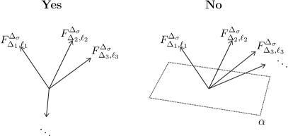
Figure 5: Left: A case where vectors can sum to zero with positive coefficients. Right: A case where vectors cannot sum to zero with positive coefficients and there exists a separating plane $\alpha$ such that all vectors point on one side of the plane. Figure from Poland and Simmons-Duffin (2016).

This observation forms the basis for the first numerical strategy of analyzing the crossing relation Rattazzi et al. (2008): input some assumption about the CFT spectrum (e.g., a gap in the scalar spectrum with all other operators satisfying unitarity bounds) and numerically search for a separating plane $\alpha$. Equivalently we can say that we are applying a linear functional $\sum_{mn}\alpha_{mn}\partial_{z}^{m}\partial_{\bar{z}}^{n}\left[\cdot\right]\big{|}_{z=\bar{z}=1/2}$ to the crossing relations and checking if it is possible to derive a contradiction. Concretely, one can look for a vector $\vec{\alpha}$ such that the scalar product is strictly positive on at least one operator whose OPE coefficient is nonzero (this may be the identity, the stress tensor, or any other operator that we assume appears in the OPE):

$$\vec{\alpha}\cdot\vec{F}^{\Delta_{\sigma}}_{\Delta_{{\cal O}^{*}},\ell_{{\cal O}^{*}}}>0\,,$$ (100)

while it is nonnegative for all other $\{\Delta_{{\cal O}},\ell_{{\cal O}}\}$ allowed by our assumptions:

$$\vec{\alpha}\cdot\vec{F}^{\Delta_{\sigma}}_{\Delta_{{\cal O}},\ell_{{\cal O}}}\geqslant 0\,.$$ (101)

Each inequality $\vec{\alpha}\cdot\vec{F}^{\Delta_{\sigma}}_{\Delta_{{\cal O}},\ell_{{\cal O}}}\geqslant 0$ identifies a half-space and their intersection carves out a convex cone.

There is still one issue before the vector $\vec{\alpha}$ can be searched for numerically – a priori there are an infinite number of allowed vectors labeled by all $\{\Delta_{{\cal O}},\ell_{{\cal O}}\}$. The first numerical bootstrap studies employed a discretization approach: namely, they discretized the set $\{\Delta_{{\cal O}},\ell_{{\cal O}}\}$ using some small spacing between allowed dimensions so that there are a finite number of linear inequalities satisfied by a finite number of unknown coefficients $\vec{\alpha}$. Then the problem becomes a standard linear programming problem and can be solved using standard algorithms. These include simplex algorithms, where one moves from vertex to vertex on the edge of the feasible region, or interior point algorithms, where one instead traverses the interior of the feasible region. Software packages that have been used in the past for this purpose are Mathematica, the GNU Linear Programming Kit (GLPK), and the IBM ILOG CPLEX Optimizer. This discretization approach is currently considered to be obsolete, although it retains pedagogical value. More efficient approaches avoiding discretization will be discussed below.

One can slightly modify the problem in order to place bounds on OPE coefficients Caracciolo and Rychkov (2010). By isolating one particular contribution ${\cal O}^{*}$ and again applying a functional $\vec{\alpha}$ one rewrites the equation as

$$\lambda_{\sigma\sigma{\cal O}^{*}}^{2}\vec{\alpha}\cdot\vec{F}^{\Delta_{\sigma}}_{\Delta_{{\cal O}^{*}},\ell_{{\cal O}^{*}}}=-\vec{\alpha}\cdot\vec{F}^{\Delta_{\sigma}}_{0,0}-\sum_{{\cal O}}\lambda_{\sigma\sigma{\cal O}}^{2}\vec{\alpha}\cdot\vec{F}^{\Delta_{\sigma}}_{\Delta_{{\cal O}},\ell_{{\cal O}}}.$$ (102)

Then by imposing the normalization condition $\vec{\alpha}\cdot\vec{F}^{\Delta_{\sigma}}_{\Delta_{{\cal O}^{*}},\ell_{{\cal O}^{*}}}=1$ and the positivity constraints $\vec{\alpha}\cdot\vec{F}^{\Delta_{\sigma}}_{\Delta_{{\cal O}},\ell_{{\cal O}}}\geqslant 0$ one obtains the upper bound $\lambda_{\sigma\sigma{\cal O}^{*}}^{2}\leqslant-\vec{\alpha}\cdot\vec{F}^{\Delta_{\sigma}}_{0,0}$. The strongest upper bound is obtained by minimizing $-\vec{\alpha}\cdot\vec{F}^{\Delta_{\sigma}}_{0,0}$, which yields an optimization problem that can be solved with linear programming algorithms, adopting the above-mentioned discretization approach or other methods discussed below. Alternatively, one can also seek lower bounds by instead imposing $\vec{\alpha}\cdot\vec{F}^{\Delta_{\sigma}}_{\Delta_{{\cal O}},\ell_{{\cal O}}}\leqslant 0$ and maximizing $-\vec{\alpha}\cdot\vec{F}^{\Delta_{\sigma}}_{0,0}$ Poland et al. (2012). However, in general it is not possible to obtain lower bounds on OPE coefficients unless the operator ${\cal O}^{*}$ is isolated in the allowed spectrum, since one could always imagine that ${\cal O}^{*}$ has a zero OPE coefficient but operators infinitesimally close to it have nonzero coefficients.

IV.1.1 Continuous primal simplex algorithm

Instead of looking for a vector $\vec{\alpha}$ with the desired positivity properties, an alternate strategy is to search directly for a set of vectors $\{\vec{F}^{\Delta_{\sigma}}_{\Delta_{{\cal O}},\ell_{{\cal O}}}\}$ appearing in Eq. (98), subject to the positivity conditions $\lambda_{\sigma\sigma{\cal O}}^{2}\geqslant 0$. This search can be viewed as a “primal” formulation of the linear program, whereas the search for $\vec{\alpha}$ described above can be viewed as the related “dual” problem. Note that in this formulation there are a continuously infinite number of possible vectors $\vec{F}^{\Delta_{\sigma}}_{\Delta_{{\cal O}},\ell_{{\cal O}}}$ in the search space. El-Showk et al. (2014b) developed a modification of Dantzig’s simplex algorithm in order to handle such a continuous search space. The essential idea is to use Newton’s method at each step of the algorithm to identify a vector to add, which is optimal over some continuous interval of scaling dimensions $\left[\Delta_{\text{min}},\Delta_{\text{max}}\right]$ and discrete set of spins $\left[0,\ell_{\text{max}}\right]$. For reasons explained in El-Showk et al. (2014b), it is necessary to perform computations at a precision higher than machine precision. This continuous simplex algorithm is one of two state-of-the art methods for the conformal bootstrap, the other one being the semidefinite programming method described below. Three implementations of this algorithm are available: a C++ code SIPSolver Simmons-Duffin (2014b) and a Python/Cython code El-Showk and Rychkov (2014) which were used for the computations in El-Showk et al. (2014b), as well as a Julia package JuliBootS Paulos (2014b).

IV.2 Semidefinite programming

While the linear programming techniques described above are adequate for crossing relations of single 4pt functions (possibly charged under some global symmetry), they are more difficult to adapt for systems of crossing relations containing multiple operators. The reason is that the resulting crossing relations for mixed correlators are no longer linear in the positive squares of OPE coefficients. The same issue arises when considering 4pt functions of spinning operators, where multiple 3pt function tensor structures exist. In these situations one can phrase the optimization problem needed to obtain bounds using the language of semidefinite programming rather than linear programming Kos et al. (2014a).

Another use of semidefinite programming Poland et al. (2012) is to avoid needing to discretize and impose a cutoff on the exchanged operator dimensions appearing in the positivity constraints such as $\vec{\alpha}\cdot\vec{F}_{\Delta_{{\cal O}},\ell_{{\cal O}}}\geqslant 0$. We will describe both of these uses of semidefinite programming, as well as how they can be combined, below.

In most applications to the bootstrap, it has proven necessary for numerical stability to solve the semidefinite programs described below at a precision higher than machine precision. The first numerical studies made use of the software SDPA-GMP Nakata (2010) (a variant of SDPA Yamashita et al. (2010)) for this purpose. The state-of-the-art is an efficient software package SDPB, described in Simmons-Duffin (2015a), which improves on the SDPA’s primal-dual interior point algorithm primarily by taking advantage of matrix block structure and parallelization. In order to set up the problems so that they can be solved by SDPB, recent studies have typically used either Mathematica notebooks, or the interfaces PyCFTBoot Behan (2017a) or cboot Ohtsuki (2016).

IV.2.1 Mixed correlators

We will illustrate the use of semidefinite programming for mixed correlators with a simple example. Consider a system of 4pt functions containing two operators $\sigma$ and $\epsilon$, where $\sigma$ is odd under a $\mathbb{Z}_{2}$ symmetry and $\epsilon$ is even. The resulting system of crossing relations for $\langle\sigma\sigma\sigma\sigma\rangle$, $\langle\sigma\sigma\epsilon\epsilon\rangle$, and $\langle\epsilon\epsilon\epsilon\epsilon\rangle$ takes the form Kos et al. (2014a)

$$0=\sum_{{\cal O}^{+}}\begin{pmatrix}\lambda_{\sigma\sigma{\cal O}}&\lambda_{\epsilon\epsilon{\cal O}}\end{pmatrix}\vec{V}_{+,\Delta,\ell}\begin{pmatrix}\lambda_{\sigma\sigma{\cal O}}\\ \lambda_{\epsilon\epsilon{\cal O}}\end{pmatrix}+\sum_{{\cal O}^{-}}\lambda_{\sigma\epsilon{\cal O}}^{2}\vec{V}_{-,\Delta,\ell}\,,$$ (103)

where the components of the vectors $\vec{V}_{\pm,\Delta,\ell}$ run over 5 independent crossing relations, ${\cal O}_{\pm}$ denote operators even/odd under $\mathbb{Z}_{2}$ symmetry, and each $\vec{V}_{+,\Delta,\ell}$ is a 5-vector of $2\times 2$ matrices:

$$\vec{V}_{-,\Delta,\ell}=\begin{pmatrix}0\\ 0\\ F_{-,\Delta,\ell}^{\sigma\epsilon,\sigma\epsilon}(z,\bar{z})\\ (-1)^{\ell}F_{-,\Delta,\ell}^{\epsilon\sigma,\sigma\epsilon}(z,\bar{z})\\ -(-1)^{\ell}F_{+,\Delta,\ell}^{\epsilon\sigma,\sigma\epsilon}(z,\bar{z})\end{pmatrix},$$

$$\vec{V}_{+,\Delta,\ell}=\begin{pmatrix}\begin{pmatrix}F^{\sigma\sigma,\sigma\sigma}_{-,\Delta,\ell}(z,\bar{z})&0\\ 0&0\end{pmatrix}\\ \begin{pmatrix}0&0\\ 0&F^{\epsilon\epsilon,\epsilon\epsilon}_{-,\Delta,\ell}(z,\bar{z})\end{pmatrix}\\ \begin{pmatrix}0&0\\ 0&0\end{pmatrix}\\ \begin{pmatrix}0&\frac{1}{2}F^{\sigma\sigma,\epsilon\epsilon}_{-,\Delta,\ell}(z,\bar{z})\\ \frac{1}{2}F^{\sigma\sigma,\epsilon\epsilon}_{-,\Delta,\ell}(z,\bar{z})&0\end{pmatrix}\\ \begin{pmatrix}0&\frac{1}{2}F^{\sigma\sigma,\epsilon\epsilon}_{+,\Delta,\ell}(z,\bar{z})\\ \frac{1}{2}F^{\sigma\sigma,\epsilon\epsilon}_{+,\Delta,\ell}(z,\bar{z})&0\end{pmatrix}\end{pmatrix}.$$ (104)

The appearing functions $F^{ij,kl}_{\pm,\Delta,\ell}$ are given in (96). One can then look for bounds by making some assumption about the spectrum and searching for a functional $\vec{\alpha}=\sum_{mn}\vec{\alpha}_{mn}\partial_{z}^{m}\partial_{\bar{z}}^{n}\left[\cdot\right]\big{|}_{z=\bar{z}=1/2}$ satisfying the properties

$$\begin{pmatrix}1&1\end{pmatrix}\vec{\alpha}\cdot\vec{V}_{+,0,0}\begin{pmatrix}1\\ 1\end{pmatrix}>0\,,$$

$$\vec{\alpha}\cdot\vec{V}_{+,\Delta,\ell}\succeq 0\quad\textrm{for all $\mathbb{Z}_{2}$-even operators with $\ell$ even,}$$

$$\vec{\alpha}\cdot\vec{V}_{-,\Delta,\ell}\geqslant 0\quad\textrm{for all $\mathbb{Z}_{2}$-odd operators.}$$ (105)

The novel feature is now that $\vec{\alpha}\cdot\vec{V}_{+,\Delta,\ell}\succeq 0$ must be a positive semidefinite $2\times 2$ matrix, which makes the search in Eq. (105) a semidefinite programming problem. Similar structure appears for more general systems of mixed/spinning correlators, where if an exchanged operator has $N$ OPE coefficients appearing in the system then the needed positivity condition will be phrased in terms of positive semidefinite $N\times N$ matrices.

IV.2.2 Polynomial approximations

A different use of semidefinite programming, relevant for both single correlators or mixed correlators, is to avoid any discretization of the exchanged operator dimensions Poland et al. (2012). We will first explain the idea for single correlators, where one imposes inequalities of the form

$$\sum_{mn}\alpha_{mn}\partial_{z}^{m}\partial_{\bar{z}}^{n}F^{\Delta_{\sigma}}_{\Delta,\ell}(z,\bar{z})\big{|}_{z=\bar{z}=1/2} \geqslant 0\,.$$ (106)

Due to the pole expansion of the conformal blocks described in Sec. III.6.4, if one keeps a finite number of poles, then by reorganizing $h_{\Delta,\ell}$ into a rational function of $\Delta$, such derivatives can be rewritten in the form (see Sec. III.6.5)

$$\partial_{z}^{m}\partial_{\bar{z}}^{n}F^{\Delta_{\sigma}}_{\Delta,\ell}(z,\bar{z})\big{|}_{z=\bar{z}=1/2}\approx\chi_{\ell}(\Delta)P_{\ell}^{mn}(\Delta)\,,$$ (107)

where $P_{\ell}^{mn}(\Delta)$ is a polynomial in $\Delta$, and $\chi_{\ell}(\Delta)$ is a positive function for all $\Delta$ and $\ell$ satisfying the unitarity bounds. The degree of the polynomial depends on the number of poles kept in the expansion of the conformal block. Then one simply needs to impose the polynomial inequalities

$$\sum_{mn}\alpha_{mn}P^{mn}_{\ell}(\Delta^{\text{min}}_{\ell}+x)\geqslant 0$$ (108)

for all $x\geqslant 0$, where the minimum dimension at each spin $\Delta^{\text{min}}_{\ell}$ depends on the assumptions being made.

Such inequalities for polynomials can be rewritten in terms of positive semidefinite matrices following a theorem of Hilbert (1888). The relevant theorem states that any polynomial $P(x)$ that is nonnegative on the interval $[0,\infty)$ can be written in the form

$$P(x)=a(x)+xb(x),$$ (109)

where $a(x)$ and $b(x)$ are sums-of-squares of polynomials. Such sums-of-squares can in turn always be expressed in the form

$$a(x)=\text{Tr}(AQ_{d_{1}}(x)),\quad b(x)=\text{Tr}(BQ_{d_{2}}(x))\,,$$ (110)

where $Q_{d}(x)\equiv[x]_{d}[x]_{d}^{T}$ is a matrix built out of the monomials $[x]_{d}=(1,x,\ldots,x^{d})^{T}$, $d_{1}=\left\lfloor\frac{1}{2}\deg P\right\rfloor$, $d_{2}=\left\lfloor\frac{1}{2}(\deg P-1)\right\rfloor$, and $A$ and $B$ are some positive semidefinite matrices.

With this rewriting, one needs to search for coefficients $\alpha_{mn}$ and positive semidefinite matrices $A_{\ell},B_{\ell}\succeq 0$ such that

$$\sum_{mn}\alpha_{mn}P^{mn}_{\ell}(\Delta^{\text{min}}_{\ell}+x)=\\ \text{Tr}(A_{\ell}Q_{d_{1}}(x))+x\text{Tr}(B_{\ell}Q_{d_{2}}(x)).$$ (111)

In practice one must also impose a cutoff on the set of included spins $0\leqslant\ell\leqslant\ell_{\text{max}}$. This search, combined with a normalization condition such as $\vec{\alpha}\cdot\vec{F}_{0,0}^{\Delta_{\sigma}}=1$, is now in the form of a semidefinite programming problem.

As explained in detail in Kos et al. (2014a), this idea can also be applied to systems of mixed or spinning correlators where exchanged operators have multiple OPE coefficients appearing in the system. In those cases, after truncating the conformal block pole expansions one imposes constraints of the form

$$\sum_{mn}\vec{\alpha}_{mn}\cdot\begin{pmatrix}\vec{P}^{(11;mn)}_{\ell}(\Delta)&\dots&\vec{P}_{\ell}^{(1N;mn)}(\Delta)\\ \vdots&\ddots&\vdots\\ \vec{P}^{(N1;mn)}_{\ell}(\Delta)&\dots&\vec{P}_{\ell}^{(NN;mn)}(\Delta)\end{pmatrix}\succeq 0$$ (112)

$$\textrm{for}\quad\Delta\geqslant\Delta^{\text{min}}_{\ell}.$$

Again there is a theorem that such positive semidefinite matrix polynomials can always be written as sums-of-squares of matrix polynomials. A consequence, worked out in Kos et al. (2014a), is that each entry can be written as

$$\sum_{mn}\vec{\alpha}_{mn}\cdot\vec{P}^{(ij;mn)}_{\ell}(\Delta^{\text{min}}_{\ell}+x)=\\ \text{Tr}(A^{ij}_{\ell}Q_{d_{1}}(x))+x\text{Tr}(B^{ij}_{\ell}Q_{d_{2}}(x))$$ (113)

in terms of positive semidefinite matrices $A_{\ell}^{ij},B_{\ell}^{ij}\succeq 0$, and the problem is again phrased as a semidefinite programming problem.

IV.3 Bounds and allowed regions

The algorithms described in the previous sections can be used to establish if a given point in the space of CFT data, parametrized by the dimensions of external operators and by assumptions on the exchanged spectrum, belongs to the region allowed by crossing and unitarity. Since the exchanged spectrum contains infinitely many operators, there are infinitely many assumptions one can test. The art of the numerical bootstrap is to choose an interesting assumption, and then to delineate as precisely as possible the allowed region corresponding to this assumption.

As we will see in the next sections, one of the most frequently asked questions is the following: given an OPE $\mathcal{O}\times\mathcal{O}$, derive an upper bound $\Delta_{\text{max}}$ on the dimension of the first operator appearing in this OPE having specified transformation properties under $SO(d)$ (and eventually under a global symmetry $G$), assuming e.g. that other operator dimensions are allowed to take any values allowed by unitarity. One can answer this question, for instance, as a function of $\Delta_{\mathcal{O}}$. This defines an allowed region with a boundary $\Delta_{\text{max}}(\Delta_{\mathcal{O}})$. Similarly, when one obtains an upper (or lower) bound on an OPE coefficient as discussed in Sec. IV.1, this represents the boundary of an allowed region. These boundaries give us a view into the intricate underlying geometry of the space of CFT data allowed by crossing and unitarity.

IV.4 Spectrum extraction

A point in the allowed region (see Sec. IV.3) is specified by external operator dimensions and by a handful of other numbers characterizing the assumptions, such as gaps on the exchanged operator spectrum. Once we ascertained that a point belongs to the allowed region, in some cases it is important to be able to go one step further and to extract an explicit solution to crossing, i.e. the whole spectrum of exchanged operator dimensions and their OPE coefficients. The precise way of doing this depends on which algorithm one uses. An important point is that we expect this solution to be non-unique inside the allowed region, but it should generically become unique on its boundary (see below).

The spectrum extraction is simplest in the primal simplex method, Sec. IV.1.1. In this case the spectrum is encoded directly in the set of basic vectors and is available in each step of the algorithm.

In the dual formulation of the linear programming method, one does not have access to the spectrum strictly inside the allowed region. However, one can extract a solution to crossing symmetry from the limiting functional when one approaches a boundary of this region, by extremizing either an operator dimension or OPE coefficient. This is called the extremal functional method, introduced in Poland and Simmons-Duffin (2011) and El-Showk and Paulos (2013).

Namely, when approaching the boundary from the disallowed region, the system is on the verge of no longer allowing a separating plane, and the vector on which we require strict positivity is degenerating into the plane. In the case of a single crossing relation where we have imposed strict positivity on the identity operator, as we approach a dimension boundary we can find a vector $\vec{\alpha}$ such that $\vec{\alpha}\cdot\vec{F}^{\Delta_{\sigma}}_{0,0}\rightarrow 0$, together with the sum rule

$$0 = \sum_{{\cal O}}\lambda_{\sigma\sigma{\cal O}}^{2}\vec{\alpha}\cdot\vec{F}^{\Delta_{\sigma}}_{\Delta_{{\cal O}},\ell_{{\cal O}}},$$ (114)

where $\vec{\alpha}\cdot\vec{F}^{\Delta_{\sigma}}_{\Delta_{{\cal O}},\ell_{{\cal O}}}\geqslant 0$ for all other possible (non-identity) operators in the spectrum. One obtains a similar condition from the OPE coefficient bound in Eq. (102) if one sets the OPE coefficient to its extremal value $\lambda_{\sigma\sigma{\cal O}^{*}}^{2}=-\vec{\alpha}\cdot\vec{F}_{0,0}^{\Delta_{\sigma}}$.

In fact, it is easy to see that in order for these sums to hold along the boundary of the allowed region, it is necessary for either $\lambda_{\sigma\sigma{\cal O}}^{2}$ to be zero or for $\vec{\alpha}\cdot\vec{F}^{\Delta_{\sigma}}_{\Delta_{{\cal O}},\ell_{{\cal O}}}$ to be zero. Thus, the zeroes of $\vec{\alpha}\cdot\vec{F}^{\Delta_{\sigma}}_{\Delta_{{\cal O}},\ell_{{\cal O}}}$ tell us the scaling dimensions and spins at which the OPE coefficients are allowed to be nonzero. The resulting extremal spectrum is generically unique El-Showk and Paulos (2013).

In the above-mentioned primal simplex method, the extremal spectrum is reached from within the allowed region, and is encoded in the set of basic vectors that remain after the algorithm terminates. That this should agree with the dual approach via extremal functionals is guaranteed by the strong duality of linear programs.

The extremal functional method for extracting the spectrum is also applicable when using semidefinite programming. In this case the extremal functional is constructed in the dual formulation. Once the extremal spectrum is known, it is straightforward to reconstruct the OPE coefficients of the exchanged operators by either directly solving the bootstrap equations after inputting the extremal spectrum or extracting them from the primal solution of the primal-dual algorithm. Simmons-Duffin (2017c) gives a precise algorithm for doing this using functionals output by SDPB, realized in a Python code Simmons-Duffin (2016a).

An important open question is to understand which CFTs are described by spectra which are extremal with respect to some extremization condition. As we will see in subsequent sections, empirically this seems to be the case for a variety of interesting CFTs including the 3d Ising and $O(N)$ models. Although it is not currently understood why it should be so, some speculations are given in Sec. V.2.3.

IV.4.1 Flow method

An interesting idea was proposed in El-Showk and Paulos (2018), where given one extremal solution one can efficiently “flow” along the boundary to reconstruct nearby extremal solutions. The idea is to perturb the extremal spectrum and then impose that the perturbed spectrum is also extremal using (114) as well as the tangency conditions $\vec{\alpha}\cdot\left(\partial_{\Delta_{{\cal O}}}\vec{F}^{\Delta_{\sigma}}_{\Delta_{{\cal O}},\ell_{{\cal O}}}\right)$. By linearizing perturbations of these conditions, the search for a nearby extremal spectrum (or a more precise extremal spectrum) can be efficiently solved using Newton’s method. This approach then avoids the use of convex optimization after the initial step of finding an initial extremal solution, and can also be used to flow to nonunitary extremal solutions. This idea was shown to work well in $d=1$ in El-Showk and Paulos (2018); Paulos et al. (2017). It appears very promising and it needs to be further explored and extended, especially into higher dimensions.

IV.5 Truncation method

Finally we wish to turn to an idea introduced by Gliozzi (2013) and explored in a variety of works, which we will call the truncation method. The basic idea is to truncate the bootstrap equations to a finite number of operators $\{\Delta_{\sigma},{\cal O}_{I}\}$ with $N$ unknown scaling dimensions. After normalizing by the identity contribution $f^{\Delta_{\sigma}}_{\Delta_{{\cal O}_{I}},\ell_{{\cal O}_{I}}}(z,\bar{z})\equiv F^{\Delta_{\sigma}}_{\Delta_{{\cal O}_{I}},\ell_{{\cal O}_{I}}}(z,\bar{z})/\left(-F^{\Delta_{\sigma}}_{0,0}(z,\bar{z})\right)$, let us write the crossing equations as

$$\sum_{{\cal O}_{I}}\lambda_{\sigma\sigma{\cal O}_{I}}^{2}f^{\Delta_{\sigma}}_{\Delta_{{\cal O}_{I}},\ell_{{\cal O}_{I}}} = 1,$$

$$\sum_{{\cal O}_{I}}\lambda_{\sigma\sigma{\cal O}_{I}}^{2}\vec{f}^{\Delta_{\sigma}}_{\Delta_{{\cal O}_{I}},\ell_{{\cal O}_{I}}} = 0.$$ (115)

Here the first equation containing $f^{\Delta_{\sigma}}_{\Delta_{{\cal O}_{I}},\ell_{{\cal O}_{I}}}\equiv f^{\Delta_{\sigma}}_{\Delta_{{\cal O}_{I}},\ell_{{\cal O}_{I}}}(1/2,1/2)$ is viewed as an “inhomogeneous” equation containing the identity contribution on the right-hand side, and the second “homogeneous” equation contains the vector of derivatives $\left(\vec{f}^{\Delta_{\sigma}}_{\Delta_{{\cal O}_{I}},\ell_{{\cal O}_{I}}}\right)^{mn}=\partial_{z}^{m}\partial_{\bar{z}}^{n}f^{\Delta_{\sigma}}_{\Delta_{{\cal O}_{I}},\ell_{{\cal O}_{I}}}(z,\bar{z})\big{|}_{z=\bar{z}=1/2}$. If one keeps $M$ derivatives with $M>N$ then the system becomes over-constrained, and only has solutions if all of the minors of order $N$ of the linear system vanish,

$$\text{det}A_{i}=0,\quad A_{i}\subset A=\left[\left(\vec{f}^{\Delta_{\sigma}}_{\Delta_{{\cal O}_{I}},\ell_{{\cal O}_{I}}}\right)^{mn}\right]_{N\times M}.$$ (116)

Here the “rows” of $A$ would run over different choices of $N$ derivatives $mn$ and the “columns” run over the $N$ unknown scaling dimensions. Note that the set of unknown scaling dimensions will include the external dimension $\Delta_{\sigma}$ in addition to the ${\cal O}_{I}$, but may exclude exchanged operators of known dimension, such as the stress tensor of known dimension $\Delta_{T}=d$. The general strategy is to solve the determinant conditions Eq. (116) to obtain an approximate spectrum of scaling dimensions, and then use the system in Eq. (IV.5), including the inhomogeneous equation, in order to fix the OPE coefficients.

A big advantage of the truncation approach over the linear and semidefinite programming approaches of the previous sections is that it does not require unitarity, i.e. it works equally well for any sign of the OPE coefficients. For example, the idea has been successfully applied to the nonunitary Lee-Yang model, as well as to bulk-boundary bootstrap problems where there is no positivity in the coefficients. Another advantage is that it is relatively simple to implement, and the idea can be explored e.g. using fairly simple Mathematica notebooks.

On the other hand, we also see several disadvantages with this approach in its current incarnation. One is that the resulting spectrum can have a strong sensitivity to the set of included operators (e.g., the choices of spins) and to the set of derivatives included. It is also very difficult to assign reliable errors to the spectrum output from the method. Thus, it would be desirable to find ways to make the approach more systematic with errors under control. Some steps in this direction were recently taken in Li (2017). Applications to the boundary bootstrap also seem to be less sensitive to these issues Gliozzi et al. (2015); Gliozzi (2016).

Another issue is that simple implementations of numerical studies of the nonlinear determinant conditions (116), such as using the iterative Newton method implemented in Mathematica’s FindRoot function, do not scale very well with increasing the number of operators and the method likely needs a more efficient numerical implementation in order to push beyond $\sim 10$ operators.

Notice that since we are truncating the spectrum, we cannot generally expect to find exact solutions of Eq. (116). On the other hand, the set of determinant conditions is in fact redundant because of the Plücker relations satisfied by the minors of a matrix, see Hikami (2017b). A cleaner numerical formulation can be obtained by replacing Eq. (116) with the problem of minimizing the smallest singular value of the matrix $A$ Esterlis et al. (2016); LeClair and Squires (2018).

Finally, similarly to the extremal spectra methods above, it is not clear which CFT spectra are “truncable” in the sense that they can be found with this approach.

V Applications in $d=3$

In this section we turn to applications of the numerical bootstrap techniques to CFTs in $d=3$ dimensions. Our discussion is organized as follows. We start in Sec. V.1 by presenting a general bound on critical vs. multicritical behavior in unitary 3d CFTs. In the following Secs. V.2 and V.3 we discuss bootstrap bounds which can be derived under the assumption of a $\mathbb{Z}_{2}$ or $O(N)$ global symmetry. Applications to the most famous 3d CFTs realizing these symmetries—the critical 3d Ising and $O(N)$ models—will be emphasized.

In Sec. V.4 we describe bounds on CFTs with fermionic operators, such as the IR fixed point of the Gross-Neveu-Yukawa models. In Sec. V.5 we discuss what the bootstrap currently has to say about CFTs realizable as IR fixed points of 3d QED coupled to matter. In Sec. V.6 we discuss recent bootstrap studies which implement crossing symmetry constraints on 4pt functions of stress tensors and conserved currents. These results are very general as they apply to any local 3d CFT. Finally, in Sec. V.7 we highlight some targets that may be interesting to look at in future numerical bootstrap studies.

While most of the results will be phrased in a way which is highly model independent and in the language of conformal field theory, we hope that we can emphasize the physical interpretation of the various assumptions that are being made. All of the results summarized in this section have been obtained under the assumption of unitarity. Nonunitary CFTs, which can be studied e.g. using the truncation method, are discussed separately in Sec. VIII.

Finally, let us remind the reader that all of the numerical results that we summarize have been obtained using a variety of methods for numerically computing conformal blocks, with different choices of tolerance parameters in linear/semidefinite programs, with different choices of the cutoff $\Lambda$ on the number of derivatives applied to the crossing relation, etc. To keep our discussion readable, we will in most cases suppress these details, which can be found described in the original studies.

V.1 Bounds on critical vs multicritical behavior

As discussed in Sec. II.1, two basic structural characteristics of any CFT are the global symmetry group $G$ and the number of relevant scalar operators $S$ which are singlets under $G$. For this discussion we will view discrete spacetime symmetries such as the spatial parity $P$, if preserved, as a part of $G$.

The importance of the number $S$ becomes clear when we try to reach the CFT as an IR fixed point of an RG flow starting from a microscopic description, which for this discussion we will assume has the full symmetry $G$. Later in Sec. V.5.3 we will comment on the situation of emergent symmetries which are not present in the microscopic description.

It follows from basic RG theory that the RG flow can reach the IR fixed point without any fine tuning if and only if $S=0$. We will call such CFTs “self-organized” by loose analogy with what happens in self-organized criticality Bak et al. (1987). Examples include QED₃ and QCD₄ in the conformal window, to be discussed in Secs. V.5 and VI.3.

On the other hand, if relevant singlet scalars are present ($S>0$), then reaching the fixed point requires fine-tuning $S$ parameters in the microscopic Lagrangian. A common case is when $S=1$, as is realized for the critical Ising model and $O(N)$ models discussed below. Then we say that we have a critical point. Finally, the case $S>1$ is classified as a multicritical point.

The simplest example of a 3d multicritical point is the free scalar field $\phi$. It has a $\mathbb{Z}_{2}$ global symmetry acting as $\phi\to-\phi$, with two relevant singlet scalars, $\phi^{2}$ and $\phi^{4}$, of dimension 1 and 2 respectively. A third singlet scalar $\phi^{6}$ has dimension exactly 3 and is marginal (it is actually marginally irrelevant). This CFT describes a tricritical 3d Ising model. Many nontrivial multicritical fixed points can be realized in systems of multiple interacting scalar fields.

Suppose that we know that we have a critical point, but not a multicritical point, i.e. that there is one and only one singlet scalar, call it ${\cal O}_{0}$. The OPE of ${\cal O}_{0}$ with itself has the schematic form

$${\cal O}_{0}\times{\cal O}_{0}\sim\mathds{1}+\lambda{\cal O}_{0}+\lambda^{\prime}{\cal O}_{0}^{\prime}+\ldots$$ (117)

where since ${\cal O}_{0}$ is a singlet it can appear on the r.h.s., we denote the next singlet scalar as ${\cal O}_{0}^{\prime}$, and $\ldots$ stands for all other operators. In this setup, Nakayama and Ohtsuki (2016) used the numerical bootstrap to derive an upper bound on the dimension of ${\cal O}_{0}^{\prime}$ as a function of dimension of ${\cal O}_{0}$, shown in Fig. 6. From this plot, the requirement $\Delta_{{\cal O}_{0}^{\prime}}>3$ translates into the lower bound

$$\Delta_{{\cal O}_{0}}>1.044\quad\text{for any critical 3d CFT.}$$ (118)

In terms of the critical exponent $\nu=1/(3-\Delta_{{\cal O}_{0}})$, this means that $\nu>0.511$ for any critical (but not multicritical) 3d fixed point described by a unitary CFT.

Among all critical 3d fixed points that we know of, the lowest $\Delta_{{\cal O}_{0}}\approx 1.41$ is realized in the critical Ising model, see below. This satisfies the above general bound (118) by a large margin.

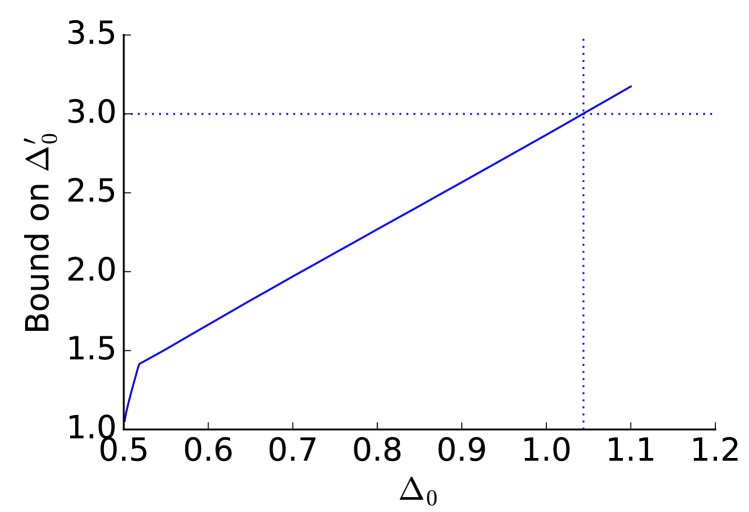
Figure 6: (Color online) Upper bound on the dimension of the second singlet scalar ${\cal O}_{0}^{\prime}$ as a function of the dimension of the first ${\cal O}_{0}$ (Nakayama and Ohtsuki, 2016, Supplementary Material).

V.2 $\mathbb{Z}_{2}$ global symmetry

V.2.1 General results

We are not aware of any unitary 3d CFTs which do not possess any global symmetry. Actually, most 3d CFTs have continuous global symmetries. Here we will start by considering the effect of having a discrete $\mathbb{Z}_{2}$, which may be a full symmetry as for the 3d Ising model, or a subgroup of a larger group.

In the CFT context, a $\mathbb{Z}_{2}$ symmetry imposes selection rules on the possible operators appearing in different OPE channels. Let us take a $\mathbb{Z}_{2}$-odd scalar operator $\sigma$ and consider the $\sigma\times\sigma$ OPE. It can only contain $\mathbb{Z}_{2}$-even operators:

$$\sigma\times\sigma\sim\mathds{1}+\lambda_{\sigma\sigma\epsilon}\epsilon+\lambda_{\sigma\sigma T}T^{\mu\nu}+\ldots.$$ (119)

Here, $\mathds{1}$ is the identity operator, $\epsilon$ is the leading $\mathbb{Z}_{2}$-even scalar, $T^{\mu\nu}$ is the stress-energy tensor, and so on. In particular, unlike in (117), $\sigma$ does not appear in the OPE.

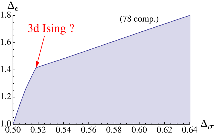
Figure 7: (Color online) Upper bound on $\Delta_{\epsilon}$ as a function of $\Delta_{\sigma}$ in 3d CFTs El-Showk et al. (2012).

In this setup, we would like to ask what is the maximal allowed value of $\Delta_{\epsilon}$. A numerical bootstrap analysis of the 4pt function function $\langle\sigma\sigma\sigma\sigma\rangle$ (via linear or semidefinite programming) produces an upper bound on $\Delta_{\epsilon}$ as a function of $\Delta_{\sigma}$, shown in Fig. 7. The point $\{1/2,1\}$ corresponds to the theory of a free massless scalar while the point $\sim\{0.518,1.413\}$, sitting near a discontinuity in the boundary, corresponds to the critical 3d Ising model which we discuss further below. Other theories that live in the interior of this region are the critical $O(N)$ models (see Sec. V.3), where we can identify $\sigma$ with a component of the $O(N)$ fundamental $\phi_{i}$ and $\epsilon$ with a component of the $O(N)$ symmetric tensor $t_{ij}$, as well as the line of mean field theory CFTs with $\Delta_{\epsilon}=2\Delta_{\sigma}$ (see Sec. III.9.1).

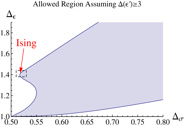
Figure 8: (Color online) Allowed region in the $\{\Delta_{\sigma},\Delta_{\epsilon}\}$ plane under the assumption that $\epsilon$ is the only relevant scalar El-Showk et al. (2012).

A particularly physically interesting class of $\mathbb{Z}_{2}$-symmetric CFTs are those with only one relevant $\mathbb{Z}_{2}$-even operator (i.e., they have $S=1$). If the microscopic realization of the theory preserves the $\mathbb{Z}_{2}$ symmetry, then this condition ensures that only one parameter must be tuned in order to reach the critical point. This allowed region in $\{\Delta_{\sigma},\Delta_{\epsilon}\}$ space was also computed in El-Showk et al. (2012) from the $\langle\sigma\sigma\sigma\sigma\rangle$ correlator, assuming that all scalars aside from the contribution at $\Delta_{\epsilon}$ are irrelevant. This region is shown in Fig. 8, with the assumption having the effect of carving into the allowed region from both the left and from the bottom.

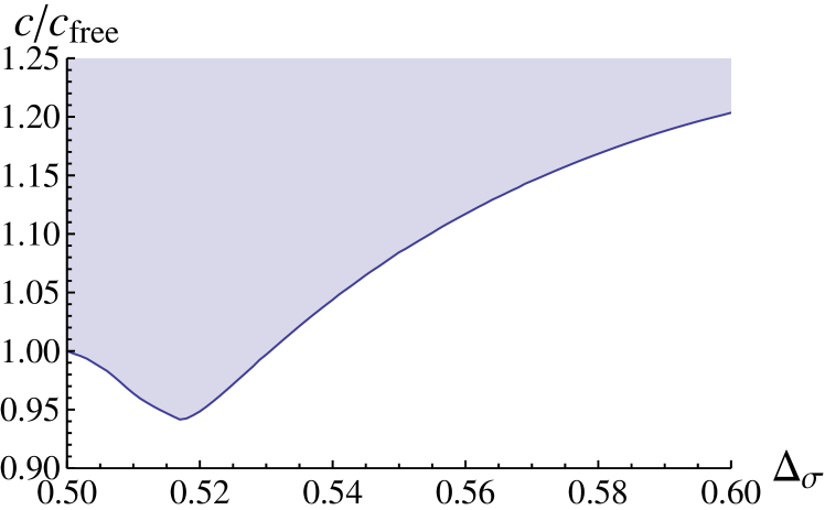
Figure 9: (Color online) Lower bound on the central charge as a function of $\Delta_{\sigma}$ El-Showk et al. (2012).

Another general result from this 4pt function is a lower bound on the central charge $C_{T}$ shown in Fig. 9, obtained by computing an upper bound on the coefficient $\lambda_{\sigma\sigma T}\propto\frac{\Delta_{\sigma}}{\sqrt{C_{T}}}$ (see Sec. III.8 and Eq. (86)). As $\Delta_{\sigma}\rightarrow 1/2$, the lower bound on $C_{T}$ approaches the free scalar value, while near the critical 3d Ising dimension $\Delta_{\sigma}\sim 0.518$, the lower bound on $C_{T}$ is seen to have a minimum. This particular bound was computed with the mild assumption $\Delta_{\epsilon}\geqslant 1$, so it is applicable to any theory living in the allowed region seen in Fig. 7.

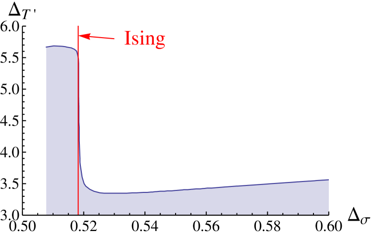
Figure 10: (Color online) Upper bound on the dimension $\Delta_{T^{\prime}}$ of the first $\mathbb{Z}_{2}$-even spin-2 operator after the stress tensor, as a function of $\Delta_{\sigma}$ El-Showk et al. (2012).

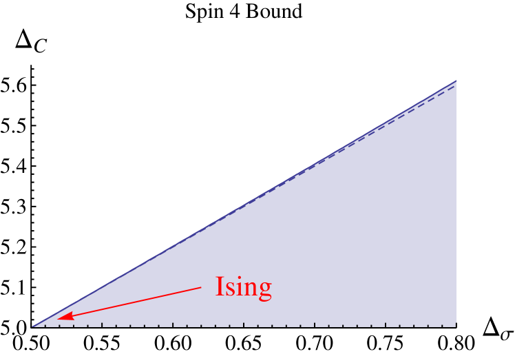
Figure 11: (Color online) Upper bound on the dimension of the leading $\mathbb{Z}_{2}$-even spin-4 operator El-Showk et al. (2012).

Before we move on to discussing what can be learned from systems of several 4pt functions, we would like to highlight that upper bounds on the leading unknown scaling dimension in other channels can also be computed and are often quite strong. For example, an upper bound on the leading unknown spin-2 dimension $\Delta_{T^{\prime}}$ (the first $\mathbb{Z}_{2}$-even spin-2 operator after the stress tensor) is shown in Fig. 10, and an upper bound on the leading spin-4 dimension $\Delta_{C}$ is shown in Fig. 11. The bound on $\Delta_{T^{\prime}}$ shows a sharp jump near the critical 3d Ising value, while no such transition is seen in the bound on $\Delta_{C}$ (which is close to being saturated by MFT: $\Delta_{C}=2\Delta_{\sigma}+4$). The jump in $\Delta_{T^{\prime}}$ shows that it is possible for the low-dimension spin-2 operator present in the spectrum for $\Delta_{\sigma}\gtrsim 0.52$ to decouple at smaller values of $\Delta_{\sigma}$. We discuss operator decoupling phenomena further in Sec. V.2.3 .

Figure 12: (Color online) Allowed region following from the analysis of three 4pt functions assuming $\Delta_{\sigma^{\prime}}\geqslant 3$ with no assumption on $\Delta_{\epsilon^{\prime}}$ Kos et al. (2014a).

Next one can ask what is the effect of adding constraints from other 4pt functions. So far the main system that has been studied in the literature is $\{\langle\sigma\sigma\sigma\sigma\rangle,\langle\sigma\sigma\epsilon\epsilon\rangle,\langle\epsilon\epsilon\epsilon\epsilon\rangle\}$, though other systems may also prove interesting. An advantage of including the correlator $\langle\sigma\sigma\epsilon\epsilon\rangle$ is that it allows one to probe the $\mathbb{Z}_{2}$-odd operators appearing in the OPE:

$$\sigma\times\epsilon\sim\lambda_{\sigma\epsilon\sigma}\sigma+\lambda_{\sigma\epsilon\sigma^{\prime}}\sigma^{\prime}+\ldots.$$ (120)

In Kos et al. (2014a) it was found that with no assumptions this system leads to an allowed region identical to Fig. 7, while by inputting the assumption of a single relevant $\mathbb{Z}_{2}$-odd operator (i.e., $\Delta_{\sigma^{\prime}}\geqslant 3$) it leads to the allowed region shown in Fig. 12. In this plot one can see a detached “island” containing the critical Ising model as well as a “bulk” region further to the right. This “bulk” region has so far not been systematically explored in the literature: it would be very interesting to understand what other CFTs lie inside of it.

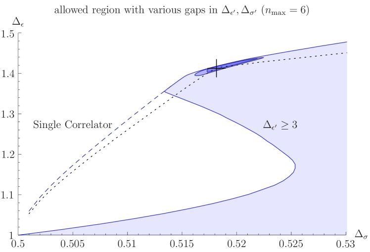
Figure 13: (Color online) This plot assumes $\Delta_{\epsilon^{\prime}}\geqslant 3$ (light blue), $\Delta_{\sigma^{\prime}}\geqslant 3$ (medium blue), or both gaps simultaneously (dark blue). Figure from Kos et al. (2014a).

In Fig. 13 we also show the difference between assuming $\Delta_{\epsilon^{\prime}}\geqslant 3$, $\Delta_{\sigma^{\prime}}\geqslant 3$, and both assumptions simultaneously. One can see that the assumption of a gap in the $\mathbb{Z}_{2}$-odd spectrum is primarily responsible for creating the detached region. In the next section we describe the connection to the critical Ising model in more detail, as well as the techniques and additional inputs that can be used to make this detached island as small as possible.

V.2.2 Critical Ising model

Perhaps the most well-known 3d CFT is the critical 3d Ising model. The study of this model has a long history Domb (1974), in part because it describes critical behavior in uniaxial magnets, liquid-vapor transitions, binary fluid mixtures, the quark-gluon plasma, and more Pelissetto and Vicari (2002). While these applications are predominantly for systems in three spatial dimensions at finite temperature, described by a 3d Euclidean CFT, the critical Ising model can also be realized as a Lorentzian (2+1)d quantum critical point Fradkin and Susskind (1978); Henkel (1984). Here we work in the Euclidean signature; the Lorentzian version is obtainable by Wick rotation and has the same set of CFT data.

In its original formulation as a model of ferromagnetism, the 3d Ising model is described using a set of spins $s_{i}=\pm 1$ on a cubic lattice in $\mathbb{R}^{3}$ with nearest neighbor interactions, with partition function

$$Z=\sum_{\{s_{i}\}}\exp\Bigl{(}-J\sum_{\langle ij\rangle}s_{i}s_{j}\Bigr{)}.$$ (121)

At a critical value of the coupling $J$, the model becomes a nontrivial CFT at long distances. Notice that the lattice model has a manifest $\mathbb{Z}_{2}$ symmetry under which $s_{i}\rightarrow-s_{i}$. This symmetry is inherited by the CFT, which contains local operators that are either even or odd under its $\mathbb{Z}_{2}$ global symmetry.

Another microscopic realization is in terms of a continuous scalar field theory in 3 dimensions, with action

$$S=\int d^{3}x\left(\frac{1}{2}(\partial\sigma)^{2}+\frac{1}{2}m^{2}\sigma^{2}+\frac{1}{4!}\lambda\sigma^{4}\right),$$ (122)

which also has a $\mathbb{Z}_{2}$ symmetry under which $\sigma\rightarrow-\sigma$. Because both $m^{2}$ and $\lambda$ describe relevant couplings, this theory is described by a free scalar at short distances but has nontrivial behavior at long distances. At a critical value of the dimensionless ratio $m^{2}/\lambda^{2}$ the long-distance behavior is described by a CFT, which is the same as for the above lattice model.

From the conformal bootstrap perspective, the Ising CFT has a $\mathbb{Z}_{2}$ global symmetry, one relevant $\mathbb{Z}_{2}$-odd scalar operator $\sigma$, and one relevant $\mathbb{Z}_{2}$-even scalar operator $\epsilon$. This is evident from experimental realizations, where $\mathbb{Z}_{2}$-preserving microscopic realizations require one tuning (e.g., tuning the temperature in uniaxial magnets) and $\mathbb{Z}_{2}$-breaking microscopic realizations require two tunings (e.g., tuning both temperature and pressure in liquid-vapor transitions). Note that the assumption that the only relevant scaling dimensions are $\Delta_{\sigma}$ and $\Delta_{\epsilon}$ is the same assumption that went into producing the dark blue detached region of Fig. 13.

Kos et al. (2016) pursued a numerical analysis of the mixed-correlator bootstrap system containing $\sigma$ and $\epsilon$ to high derivative order. In addition, they studied the impact of scanning over different possible values of the ratio $\lambda_{\epsilon\epsilon\epsilon}/\lambda_{\sigma\sigma\epsilon}$. This scan effectively inputs the information that there is a single operator in the OPE occurring at the scaling dimension $\Delta_{\epsilon}$, whereas the plot of Fig. 13 allowed for the possibility of multiple degenerate operator contributions at the dimension $\Delta_{\epsilon}$. This led to the three-dimensional allowed region shown in Fig. 14 and its projection to the $\{\Delta_{\sigma},\Delta_{\epsilon}\}$ plane shown in Fig. 15. In addition, for each point in this region the magnitude of the leading OPE coefficients were also bounded, with the result shown in Fig. 16. These world-record numerical determinations are summarized below in Table. 2.

Finally let us mention that recent studies of the conformal bootstrap for stress-tensor 4pt functions have also made contact with the 3d Ising model. In particular, after inputting known values of the leading parity-even spectrum, Dymarsky et al. (2018) gave a new bound on the leading parity-odd $\mathbb{Z}_{2}$-even scalar, $\Delta_{\text{odd}}<11.2$, and constrained the independent coefficient in the stress-tensor 3pt function (parametrized by the variable $\theta$) to be in the range $0.01<\theta<0.05$ if $\Delta_{\text{odd}}>3$ and in a tighter range $0.01<\theta<0.018-0.019$ if $\Delta_{\text{odd}}$ is close to saturating its bound. We will discuss these constraints in more detail in Sec. V.6.

Figure 14: (Color online) Allowed region in the $\{\Delta_{\sigma},\Delta_{\epsilon},\lambda_{\epsilon\epsilon\epsilon}/\lambda_{\sigma\sigma\epsilon}\}$ space obtained in Kos et al. (2016).

Figure 15: (Color online) Projection of the 3d region in Fig. 14 on the $\{\Delta_{\sigma},\Delta_{\epsilon}\}$ plane and its comparison with a Monte Carlo prediction for the same quantities Kos et al. (2016).

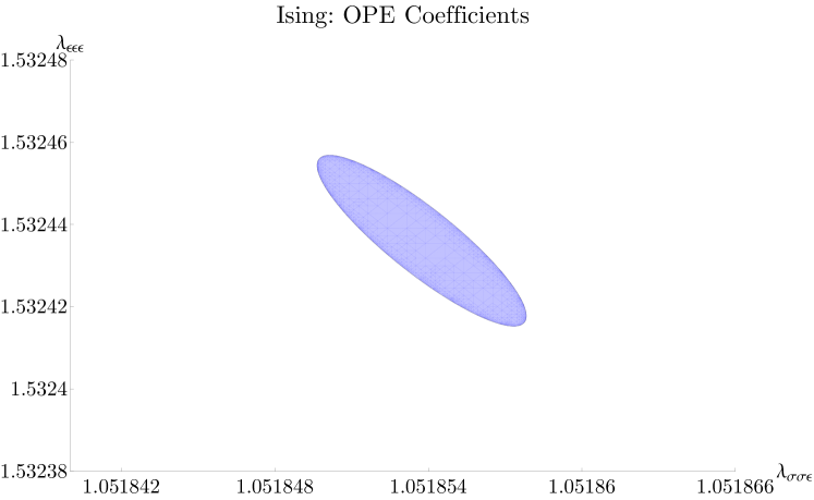
Figure 16: (Color online) Variation of $\lambda_{\epsilon\epsilon\epsilon}$ and $\lambda_{\sigma\sigma\epsilon}$ within the allowed region in Fig. 14 Kos et al. (2016).

V.2.3 Spectrum extraction and rearrangement

We have seen in the previous section the remarkable precision with which the leading scaling dimensions of the critical 3d Ising model can be determined. This raises the immediate question of how well we can extract other operator dimensions and OPE coefficients in the spectrum using bootstrap methods (specifically the strategies described in Sec. IV.4)

Even prior to the mixed-correlator studies mentioned above, El-Showk et al. (2014b) extracted the spectrum using the primal simplex method strategy, from a solution to crossing for the $\langle\sigma\sigma\sigma\sigma\rangle$ correlator which minimizes the central charge $C_{T}$. For example, Fig. 17 shows the scalar operators in the extracted spectrum as a function of $\Delta_{\sigma}$ near the 3d Ising model. A fascinating feature of these plots is the bifurcation of operators that occurs at the Ising value of $\Delta_{\sigma}$, which can be interpreted as a decoupling of one of the operators in the spectrum. This “spectrum rearrangement” phenomenon has yet to be fully understood, but speculatively it could be connected to the nonperturbative equations of motion (i.e., the 3d analogue of the relation $\sigma\partial^{2}\sigma\sim\sigma^{4}$ at the Wilson-Fisher fixed point) or a higher-dimensional extension of the null state conditions in the 2d Ising CFT (see also Sec. V.2.4).

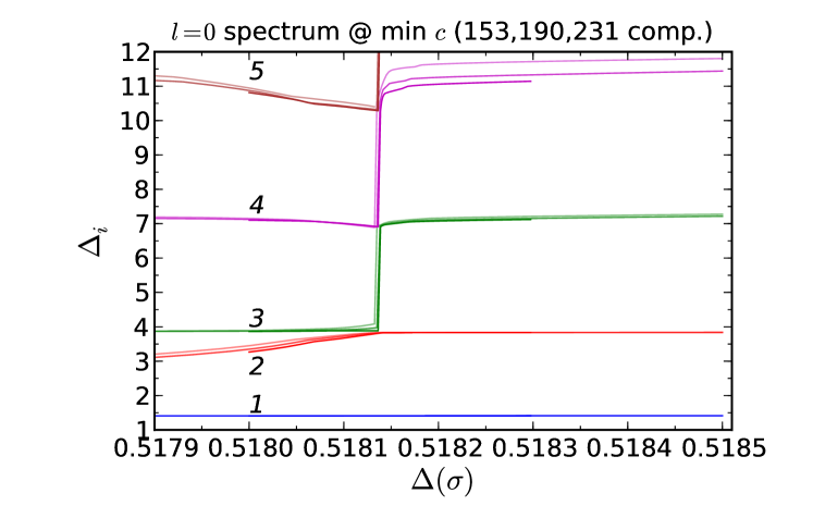
Figure 17: (Color online) The spectrum of $\mathbb{Z}_{2}$-even scalar operators appearing in the solution to crossing minimizing $C_{T}$ near $\Delta_{\sigma}$ corresponding to the 3d Ising model El-Showk et al. (2014b). Line 1 corresponds to the $\epsilon$ operator and shows little variation on the scale of this plot. All other lines exhibit the spectrum rearrangement phenomenon.

On the other hand, spectrum extraction using the extremal functional method was applied to the critical 3d Ising model by Komargodski and Simmons-Duffin (2017); Simmons-Duffin (2017c). In the latter work, for a set of 20 trial points distributed within the island of Fig. 14, $C_{T}$-minimization was performed and the zeros of the extremal functional were found. While some zeros jump significantly when moving from point to point, many of them are found to be present in all families with tiny variations. About a hundred such “stable zeros” were identified, and are believed to represent operators which truly exist in the 3d Ising CFT, providing a remarkable view of the spectrum of this theory. The subset of stable operators with dimensions $\Delta\leqslant 8$, and their OPE coefficients, are shown in Table 2.

This approach, while not fully rigorous, is intuitively justified as a means to extend the reach of rigorous analysis which produced the island in Fig. 14. The errors on stable operator dimensions and OPE coefficients are assigned as standard deviations in the set of trial points. Although these errors are not rigorous, as opposed to rigorous errors implied by Figs. 14, 15, and 16, we believe that they represent realistic estimates. In future studies the error estimates can be further checked by enlarging the set of trial points and by extremizing multiple quantities as opposed to just $C_{T}$.

Results of this approach for the leading towers of low-twist operators (of increasing spin) have also been tested against the analytical bootstrap computations in the lightcone limit which yield analytical expressions for the large-spin asymptotics. In Fig. 18, the data points extracted from the extremal functional approach show the leading twist ($\tau=\Delta-\ell$) trajectory in the $\hbox{$Z$}_{2}$-even sector as a function of $\bar{h}=\ell+\tau/2$, while the curve shows the analytical computation, displaying excellent agreement with the data even down to small spins. Similar good agreement was also found with the extracted OPE coefficients and subleading trajectories, as well as in the $\hbox{$Z$}_{2}$-odd sector.

We also report here the prediction for the central charge from the above $C_{T}$-minimization over the 20 points in the island Simmons-Duffin (2017a):

$$C^{\rm Ising}_{T}/C_{T}^{\text{free boson}}=0.9465389(12)\,,$$ (123)

improving the previous $C_{T}$-minimization determination by El-Showk et al. (2014b).

${\cal O}$	$\hbox{$Z$}_{2}$	$\ell$	$\Delta$	$f_{\sigma\sigma{\cal O}}$	$f_{\epsilon\epsilon{\cal O}}$
$\epsilon$	$+$	0	$1.412625{\bf\boldsymbol{(}10\boldsymbol{)}}$	$1.0518537{\bf\boldsymbol{(}41\boldsymbol{)}}$	$1.532435{\bf\boldsymbol{(}19\boldsymbol{)}}$
$\epsilon^{\prime}$	$+$	0	$3.82968(23)$	$0.053012(55)$	$1.5360(16)$
	$+$	0	$6.8956(43)$	$0.0007338(31)$	$0.1279(17)$
	$+$	0	$7.2535(51)$	$0.000162(12)$	$0.1874(31)$
$T_{\mu\nu}$	$+$	2	$3$	$0.32613776(45)$	$0.8891471(40)$
$T^{\prime}_{\mu\nu}$	$+$	2	$5.50915(44)$	$0.0105745(42)$	$0.69023(49)$
	$+$	2	$7.0758(58)$	$0.0004773(62)$	$0.21882(73)$
$C_{\mu\nu\rho\sigma}$	$+$	4	$5.022665(28)$	$0.069076(43)$	$0.24792(20)$
	$+$	4	$6.42065(64)$	$0.0019552(12)$	$-0.110247(54)$
	$+$	4	$7.38568(28)$	$0.00237745(44)$	$0.22975(10)$
	$+$	6	$7.028488(16)$	$0.0157416(41)$	$0.066136(36)$
${\cal O}$	$\hbox{$Z$}_{2}$	$\ell$	$\Delta$	$f_{\sigma\epsilon{\cal O}}$	-
$\sigma$	$-$	0	$0.5181489{\bf\boldsymbol{(}10\boldsymbol{)}}$	$1.0518537{\bf\boldsymbol{(}41\boldsymbol{)}}$
$\sigma^{\prime}$	$-$	0	$5.2906(11)$	$0.057235(20)$
	$-$	2	$4.180305(18)$	$0.38915941(81)$
	$-$	2	$6.9873(53)$	$0.017413(73)$
	$-$	3	$4.63804(88)$	$0.1385(34)$
	$-$	4	$6.112674(19)$	$0.1077052(16)$
	$-$	5	$6.709778(27)$	$0.04191549(88)$

Table 2: Stable operators in the critical 3d Ising model with dimensions $\Delta\leqslant 8$ Simmons-Duffin (2017c). Conventional names are shown in the leftmost column when available. Errors in bold are rigorous. All other errors are non-rigorous but, in our opinion, realistic. See Eq. (123) for the central charge prediction from the same study. Because we have chosen a different conformal block normalization convention, the OPE coefficients are related to our convention by $\lambda_{ij{\cal O}}=2^{\ell/2}f_{ij{\cal O}}$ (see Table 1).

Figure 18: (Color online) Comparison of the extremal functional spectrum with the analytic bootstrap Simmons-Duffin (2017c); see the text.

V.2.4 Why kink? Why island?

One may be wondering why the 3d Ising model happens to live at a kink in Fig. 7. Plausibly, this has to do with the minimality of the spectrum of exchanged operators required to satisfy the crossing relation. In the interior of the allowed region in Fig. 7, the solution to crossing is not unique. When working numerically, a typical solution contains as many operators as the number of derivatives at $z=\bar{z}=1/2$ one is keeping in (98), (99). On the other hand, when one approaches the boundary of the allowed region in Fig. 7, the nature of the solution changes in that the operators first organize into pairs with nearby dimensions, and the pairs then merge into single operators at the boundary El-Showk et al. (2014b). Thus the extremal solutions to crossing are quite economical, containing many fewer operators than the interior solutions, roughly by a half.

Further reduction of the spectrum occurs at the kink. When one approaches the kink moving along the boundary, squared OPE coefficients of certain operators tend to zero. Further analytic continuation of the solution beyond the kink would be inconsistent with unitarity. Thus two different solution branches meet at the kink El-Showk et al. (2014b), and the spectrum exhibits rearrangement phenomena mentioned in Sec. V.2.3.

To summarize, that the 3d Ising model lives at a kink suggests that it is a CFT with a particularly minimal spectrum of operators. If this idea can be made precise, perhaps it can pave the way to an exact solution.

Leaving the kink aside, let us discuss the island. It is perhaps not surprising that considering crossing for several 4pt functions the allowed region shrinks compared to what was allowed when considering just one 4pt function. It is however altogether unexpected and remarkable that considering only three 4pt functions, plus a physically motivated and robust assumption of only two relevant operators, allows one to produce the tiny island shown in Figs. 12 and 15.

It is not currently understood why this happens. Would the island continue to shrink indefinitely with increasing the number of included derivatives? Or would it stabilize, requiring one to add further correlators to fully fix the CFT? More generally, is it sufficient to include only 4pt functions of relevant operators or are external irrelevant operators also needed to have a unique solution? These are fascinating questions for the future.

We will see many kinks and islands in the subsequent sections of this review, about which similar considerations can be made.

V.2.5 Nongaussianity

Since the leading spectrum and OPE coefficients of the critical 3d Ising model are now known to a high degree of precision, it is possible to reconstruct the full 4pt function $\langle\sigma\sigma\sigma\sigma\rangle$ over a wide range of cross ratios. One can then probe the question of how much this 4pt function deviates from the “gaussian”, i.e. fully disconnected, form $\langle\sigma\sigma\sigma\sigma\rangle=\langle\sigma\sigma\rangle\langle\sigma\sigma\rangle+\text{perms}$. This question is also motivated by the fact that the Ising model contains higher-spin operators with dimensions that deviate by a small amount from those of higher-spin currents, see Fig. 18. The first two of these operators are the $\mathbb{Z}_{2}$-even spin-4 and spin-6 operators in Table 2, of dimension close to 5 and 7 respectively.

Rychkov et al. (2017) probed this question quantitatively using bootstrap data to reconstruct the ratio $Q(z,\bar{z})=\frac{g(z,\bar{z})}{1+(z\bar{z})^{\Delta_{\sigma}}+(z\bar{z}/(1-z)(1-\bar{z}))^{\Delta_{\sigma}}}$ in the critical 3d Ising model, where the denominator corresponds to the “gaussian” expectation. A plot of this deviation over a fundamental domain in the complex $z$ plane is shown in Fig. 19. They found e.g. that $Q<0.75$ over a wide range of cross-ratio space and that it attains a minimum value of $Q_{\min}\approx 0.683$. Thus, any attempt to explain the small anomalous dimensions of higher-spin operators must account for this significant nongaussianity.

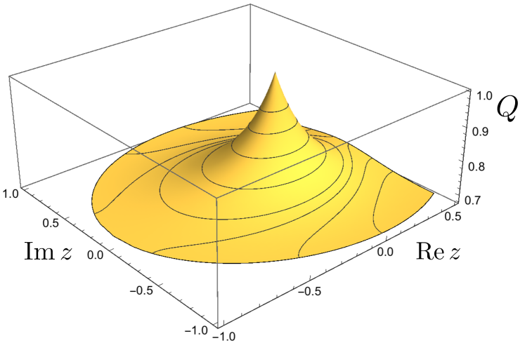
Figure 19: (Color online) The nongaussianity ratio $Q$ in the critical 3d Ising model Rychkov et al. (2017).

V.2.6 Boundary and defect bootstrap, nontrivial geometries, off-criticality

It is also interesting to study the physics of defects in the 3d Ising model. These include both co-dimension one defects (e.g., flat 2d boundaries or interfaces) and co-dimension two defects (i.e., 1d line defects). Here we would like to highlight for the reader some recent numerical bootstrap studies of such defects.

Bootstrap constraints in the 3d Ising model in the presence of a flat 2d boundary were first studied using linear programming techniques in Liendo et al. (2013), where a number of rigorous bounds were placed on the scaling dimensions and OPE coefficients of boundary operators for different choices of boundary conditions, corresponding to the “special” and “extraordinary” transitions, assuming positivity of the bulk channel expansion coefficients. Estimates of the leading boundary data using the truncation method were also computed by Gliozzi et al. (2015) and Gliozzi (2016), where precise estimates applicable to the boundary condition of the “ordinary” transition could also be made.

Studies have also been performed of the $\mathbb{Z}_{2}$ twist line defect in the 3d Ising model, constructed on the lattice by reversing the Ising coupling on a semi-infinite half-plane. The 1d boundary of this half-plane then yields the twist line defect, which can also be defined in terms of its simple monodromy properties. Local operators living on this defect were studied using both Monte Carlo techniques Billò et al. (2013) and numerical bootstrap (linear programming) techniques Gaiotto et al. (2014), with excellent agreement.

A related line of inquiry is to study CFTs such as the critical 3d Ising model on nontrivial geometries, the nontrivial case being manifolds not globally conformally equivalent to infinite flat space. This is motivated in part by the search for a higher-dimensional analogue of modular invariance. One concrete realization has been to study the 3d Ising model on real projective space Nakayama (2016c). In this case the unknown coefficients in one-point functions of scalar primary operators $\langle\mathcal{O}\rangle\propto A_{\mathcal{O}}$ enter into a variant of the bootstrap equations called the cross-cap bootstrap equations. Numerical truncation studies of the cross-cap bootstrap equations in this work have yielded new nontrivial predictions, e.g. $A_{\epsilon}=0.667(2)$ and $A_{\epsilon^{\prime}}=0.896(5)$ in the critical 3d Ising model on real projective space. Another interesting geometry is $S^{1}\times\mathbb{R}^{d-1}$, which corresponds to putting the CFT at finite temperature. This was studied for the 3d Ising model and other higher-dimensional CFTs in Iliesiu et al. (2018a). Gobeil et al. (2018) also discussed a generalization of the conformal block concept relevant for this geometry.

Let us finally mention an interesting study Caselle et al. (2016) which combined the knowledge of the 3d Ising model CFT data acquired by the bootstrap with conformal perturbation theory. They achieved a remarkable agreement with the experimental data describing the 2pt function $\langle\sigma\sigma\rangle$ off criticality, i.e. at temperatures slightly different from the critical temperature, which corresponds to perturbing the CFT by a $\int d^{3}x\,\epsilon(x)$ perturbation.

V.3 $O(N)$ global symmetry

Most known unitary 3d CFTs have a continuous global symmetry, and we now turn to such CFTs. We will focus on bootstrap results obtained by assuming $O(N)$ as a full symmetry or as a subgroup.

V.3.1 General results

As discussed in Sec. III.7, correlation functions of CFT operators that are in irreducible representations of the global symmetry $G$ can be organized using group theory and decomposed into different $G$-invariant tensor structures. Sec. III.9 explained how these structures enter the crossing relations. The first numerical analyses of the resulting equations occurred in the context of 4d CFTs, but the group theoretic structure is $d$-independent. The bootstrap for $O(N)$ symmetry in 3d was investigated by Kos et al. (2014b, 2015b, 2016) and Nakayama and Ohtsuki (2014b).

We will start our analysis assuming that the CFT contains an operator $\phi\equiv(\phi_{a})_{a=1}^{N}$ in the fundamental representation of $O(N)$, of dimension $\Delta_{\phi}$. Mimicking the discussion in Sec. V.2.1, we would like to learn about the operators in the OPE $\phi_{a}\times\phi_{b}$. By group theory, operators of even spin $\ell$ in this OPE will transform as $O(N)$ singlets or symmetric traceless tensors of rank 2, while odd-spin operators will transform in the rank-2 antisymmetric representation.

From the crossing relations for the 4pt function of $\phi$ one can put upper bounds on the dimensions of various operators. For the lowest dimension scalars ($\ell=0$) in the singlet ($s$) and symmetric traceless tensor ($t$) sector, these bounds are shown in Figs. 20, 21 as a function of $\Delta_{\phi}$ for various values of $N$. The “kinks” in these bounds will be interpreted in the next section.

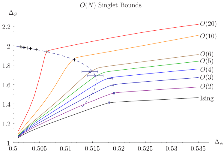
Figure 20: (Color online) Upper bound on the dimension of $s$ Kos et al. (2014b).

Figure 21: (Color online) Upper bound on the dimension of $t$ Kos et al. (2014b).

The $\phi\times\phi$ OPE also contains two interesting operators of spin $\ell\geqslant 1$: the stress tensor $T$ and the conserved current $J$. Using the bootstrap one can put lower bounds on their two-point function coefficients $C_{T}$ and $C_{J}$ (defined in Sec. III.8) given in Figs. 22, 23. This is done by bounding from above the OPE coefficients $\lambda_{\phi\phi T}\propto\Delta_{\phi}/\sqrt{C_{T}}$ and $\lambda_{\phi\phi J}\propto 1/\sqrt{C_{J}}$ (see Eqs. (86, 90)).

Let’s discuss the monotonicity of these bounds with $N$. Since $O(N+1)\supset O(N)$, the bounds on $C_{T}$, $C_{J}$, and on $\Delta_{t}$ should get stronger with increasing $N$, and indeed they do (notice that $C_{T}$ is plotted divided by $N$). Although it may seem counterintuitive that the $\Delta_{s}$ bound gets weaker with $N$, there is no contradiction. The point is that the symmetric traceless tensor of $O(N+1)$ contains a singlet $\tilde{s}$ when decomposed with respect to $O(N)$. Therefore the only constraint is that the $O(N)$ singlet bound should be weaker than the $O(N+1)$ symmetric traceless bound, which is satisfied by inspection.

Notice also that the scaling of the $C_{T}$, $C_{J}$ bounds with $N$ close to $\Delta_{\phi}=1/2$ is consistent with the fact that in the theory of $N$ free scalars, $C_{T}$ grows linearly with $N$ while $C_{J}$ is constant.

Figure 22: (Color online) Lower bound on $C_{T}$ computed under the assumption $\Delta_{s},\Delta_{t}\geqslant 1$ Kos et al. (2014b).

Figure 23: (Color online) Lower bound on $C_{J}$ Nakayama and Ohtsuki (2014b).

V.3.2 Critical $O(N)$ model

The most famous 3d CFT with $O(N)$ symmetry is the critical point of the $O(N)$ lattice model, which is the generalization of Eq. (121) to $N$-component spins satisfying the constraint $|\vec{s}|=1$. This CFT is also known as the Wilson-Fisher fixed point, being an IR fixed point of the $O(N)$ symmetric scalar field theory with quartic interaction Wilson and Fisher (1972). For any integer $N$ this 3d CFT is unitary, given that the microscopic realizations are unitary.

It’s natural to ask where the critical $O(N)$ models lie in the parameter space of $O(N)$ symmetric CFTs allowed by the general bounds from the previous section. In the Wilson-Fisher description, $\phi_{a}$ is the fundamental scalar field appearing in the Lagrangian, $s=\phi^{2}$, and $t$ is the traceless part of $\phi_{a}\phi_{b}$. Dimensions of these fields have been previously estimated using RG methods (in particular the $\epsilon$-expansion and the large $N$ expansion), Monte Carlo studies, and experiments. Comparing the $s$ and $t$ bounds and these prior determinations, marked with crosses in Figs. 20, 21, one is led to conjecture that the critical $O(N)$ models correspond to the “kinks”. Similar kink-like features are visible in the lower bounds on $C_{J}$ and $C_{T}$. In the latter case the kinks can be made sharper by imposing that the $S$ operator saturate the gap, see Fig. 5 in Kos et al. (2014b). This conjecture can be used to extract values of the $\phi$, $s$, $t$ dimensions and of $C_{T}$, given in Table 3 of Kos et al. (2014b).

We will now discuss how to isolate the critical $O(N)$ models without relying on the kink conjecture. The idea is to exploit the crucial physical feature of these CFTs — that they possess robust gaps in the operator spectrum. The singlet scalar $s$ corresponds to the temperature deformation of the critical point and is relevant. The next singlet scalar, $s^{\prime}$, must necessarily be irrelevant (otherwise the critical point would be multicritical), implying the gap $\Delta_{s^{\prime}}\geqslant 3$ in the singlet scalar sector. We also expect a gap in the fundamental representation scalar sector. The order parameter $\phi_{a}$ belongs to this sector and is relevant, while most likely the next fundamental scalar is irrelevant: $\Delta_{\phi^{\prime}}\geqslant 3$. This can be also deduced using the Wilson-Fisher description, using a nonrigorous but suggestive equation of motion argument Kos et al. (2015b).

Kos et al. (2015b) studied bootstrap constraints for the system of three correlators $\{\langle\phi_{a}\phi_{b}\phi_{c}\phi_{d}\rangle$, $\langle\phi_{a}\phi_{b}ss\rangle$, $\langle ssss\rangle\}$. Imposing the assumptions $\Delta_{s^{\prime}}\geqslant 3$, $\Delta_{\phi^{\prime}}\geqslant 3$, they found small allowed regions (“islands”) shown in Fig. 24. Improved versions of these islands for $O(2)$ and $O(3)$, discussed in the next sections, were subsequently obtained in Kos et al. (2016). It’s important to stress that, like in Fig. 12 for the Ising model, there are disconnected allowed regions outside the shown part of the parameter space; see e.g. Fig. 25 below for the $O(2)$ case. These regions are practically unexplored and they might contain other interesting CFTs.

Figure 24: (Color online) The $O(N)$ archipelago Kos et al. (2015b).

V.3.3 $O(2)$ global symmetry

We finally wish to discuss separately specific values of $N$, starting with $O(2)\supset U(1)$. There are many physically interesting 3d CFTs possessing $O(2)$ or $U(1)$ symmetry. The most famous of these is the critical $O(N)$ model for $N=2$, also known as the critical $XY$ model. It describes, in particular, the Curie point of easy-plane ferromagnets, and of easy-plane antiferromagnets on bipartite lattices. Here the $O(2)$ symmetry arises as the symmetry of local magnetic moment interactions.

Another frequent appearance of $U(1)$ symmetry in condensed matter physics is as particle number conservation. The most famous such $U(1)$ transition is the superfluid transition in ⁴He. Another example is the superfluid-insulator quantum phase transition in the (2+1)d Bose-Hubbard model at integer particle density Fisher et al. (1989). Both these transitions are also described by the critical $O(2)$ model.

A wide class of CFTs with $U(1)$ global symmetry are IR fixed points of theories which at the microscopic level contain $U(1)$ gauge fields coupled to fermion or scalar matter. The global $U(1)$ symmetry in these theories is topological in origin, and the local operators charged under it are monopoles of the gauge field. These CFTs often appear in condensed matter applications; they will be discussed in more detail in Sec. V.5.

Here we discuss general constraints from the multiple correlator bootstrap for $U(1)$ symmetric CFTs, which have been pursued further than in the general $O(N)$ case discussed above.

Operators in $U(1)$ theories are classified by their $U(1)$ charge, with $s,\phi,t$ of the previous section having charge $0,1,2$. Imposing the constraints that there is a unique relevant charge 1 and a unique relevant charge 0 scalar, one gets the allowed region shown in dark blue in Fig. 25. Notice that this region consists of a detached island to which the critical $O(2)$ model belongs, and a further region on the right, similar to Fig. 12 for the Ising model.

The island containing the critical $O(2)$ model has been studied more accurately in Kos et al. (2016) by increasing the derivative order and performing a scan over the OPE coefficient ratio $\lambda_{sss}/\lambda_{\phi\phi s}$. This led to the improved constraints shown in Fig. 26. The resulting dimensions and OPE coefficients are given in Table 3.

In the same table we give the determinations of $\Delta_{t}$ and $C_{J}$ obtained in Kos et al. (2015b) by scanning over the allowed island in the $\{\Delta_{\phi},\Delta_{s}\}$ plane, under the respective assumptions that $\Delta_{t^{\prime}}\geqslant 3$ and $\Delta_{J^{\prime}}\geqslant 3$.

These results are compatible but somewhat less precise in the case of $\Delta_{\phi}$, $\Delta_{s}$, $\Delta_{t}$ than other available determinations by lattice and RG methods, see Kos et al. (2015b, 2016) for references. In particular, a further increase in precision is required to resolve the discrepancy between the experimental and theoretical determinations of $\Delta_{s}$ shown in Fig. 26. This is an important problem for the future. On the other hand, the bootstrap is currently the only source of information about the OPE coefficients $\lambda_{\phi\phi s}$ and $\lambda_{sss}$. The central charge $C_{J}$ is related to the zero-temperature (or high-frequency) conductivity of the quantum critical points described by the critical $O(2)$ model. Although not yet experimentally measured, this parameter has been extensively studied theoretically and numerically in the condensed matter literature. As discussed in Kos et al. (2015b), the bootstrap currently provides the best determination of $C_{J}$.

Figure 25: (Color online) Allowed regions in the parameter space of $O(2)$ or $U(1)$ symmetric CFTs Kos et al. (2015b). The strongest constraint (dark blue) has been obtained from the analysis of three correlators $\{\langle\phi\phi\phi\phi\rangle$, $\langle\phi\phi ss\rangle$, $\langle ssss\rangle\}$, assuming that $s$, $\phi$ are the only two relevant scalars of charge 0, 1, and imposing the OPE coefficient relation $\lambda_{\phi\phi s}=\lambda_{\phi s\phi}$.

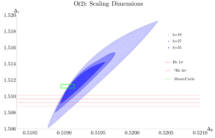
Figure 26: (Color online) Allowed islands in the mixed correlator analysis of $O(2)$ or $U(1)$ symmetric CFTs after performing a scan over the OPE coefficient ratio $\lambda_{sss}/\lambda_{\phi\phi s}$ Kos et al. (2016).

	$O(2)$	$O(3)$
$\Delta_{\phi}$	0.51926(32)	0.51928(62)
$\Delta_{s}$	1.5117(25)	1.5957(55)
$\lambda_{sss}/\lambda_{\phi\phi s}$	1.205(9)	0.953(25)
$\lambda_{\phi\phi s}$	0.68726(65)	0.5244(11)
$\lambda_{sss}$	0.8286(60)	0.499(12)
$\Delta_{t}$	1.2357(33)	1.210(6)
$C_{J}/C_{J}^{\rm free}$	0.9050(16)	0.9065(27)

Table 3: Bootstrap results for the operator dimensions and OPE coefficients in the critical $O(2)$ and $O(3)$ models (see Secs. V.3.3, V.3.4).

V.3.4 $O(3)$ global symmetry

We will now specialize to the case of $O(3)$ global symmetry, focusing on the most famous such CFT which is the critical $O(3)$ model. Apart from describing the critical point of isotropic ferromagnets, the same CFT also describes the $(2+1)$d quantum critical point in coupled dimer antiferromagnets, see Sachdev (2004) and references therein.

The bootstrap analysis of this theory mimics the $U(1)$ case from the previous section. Under the assumption that $\phi_{a}$ and $s$ are the only two relevant scalars transforming in the fundamental and trivial representation of $O(3)$, Kos et al. (2016) found an island allowed by the bootstrap constraints, shown in Fig. 27. The bootstrap determinations of the scaling dimensions and OPE coefficients following from this analysis are given in Table 3. As for the $U(1)$ case, the scaling dimension determinations are compatible but somewhat less precise than the best available Monte Carlo and RG results.

Figure 27: (Color online) The $O(3)$ analogue of Fig. 26 Kos et al. (2016).

One long-standing question about the critical $O(3)$ model concerns its stability with respect to perturbations which may potentially lead to two different CFTs, the so-called cubic and biconical fixed points, which have symmetries $B_{3}=S_{3}\rtimes(\mathbb{Z}_{2})^{3}$ and $O(2)\times\mathbb{Z}_{2}$ respectively. These perturbations take the form $K^{ijkl}\Phi_{ijkl}$, where $\Phi$ is a scalar operator transforming in the rank-4 symmetric traceless representation of $O(3)$, and $K$ is a constant tensor breaking $O(3)$ to one or the other subgroup. RG calculations indicate that the $O(3)$ fixed point is unstable while the cubic and biconical fixed points are stable, with the correction to scaling critical exponents $\omega_{O(3)}=-0.013(6)$ and $\omega_{B_{3}}=0.010(4)$ or 0.015(2) according to two calculations; see (Pelissetto and Vicari, 2002, sections 11.3, 11.7) and references therein. This would imply that $\Delta_{\Phi}=3+\omega_{O(3)}$ is very weakly relevant. From the bootstrap point of view, $\Phi$ appears in the OPE $t\times t$, and its dimension could be determined by an analysis involving correlators of $t$. This is an interesting problem for the future.

Let us mention another 3d CFT with an $O(3)$ global symmetry — the critical Gross-Neveu-Heisenberg (GNH) model Herbut et al. (2009), realized as the IR fixed point of a microscopic Lagrangian with Yukawa and quartic couplings

$$g\bar{\Psi}\sigma^{i}\phi_{i}\Psi+\lambda(\phi_{i}^{2})^{2}\,,$$ (124)

where $\phi_{i}$ is a three-component scalar order parameter, and $\Psi$ is a two-component multiplet of massless Dirac fermions. This CFT is believed to describe the continuum limit of the Hubbard model on the honeycomb and $\pi$-flux lattices Sachdev (2010). While clearly distinct from the critical $O(3)$ model, the scalar sector of this theory would be subject to the general $O(3)$ bounds shown in Figs. 20-23. However the expected value of $\Delta_{\phi}\approx 0.85$ (Parisen Toldin et al., 2015, Eq. (25)) puts it outside of the region explored so far. The fermionic sector of this theory could be constrained by methods from the next section.

V.4 CFTs with fermion operators

V.4.1 Models

The preceding sections discussed constraints from crossing relations for 4pt functions of scalar operators. Many 3d or (2+1)d CFTs of theoretical and experimental interest also contain fermionic operators, and here we will discuss what the bootstrap has so far been able to say about them.

Perhaps the simplest example is the family of CFTs described by the Gross-Neveu model at criticality Gross and Neveu (1974). While the critical theory is often described as the UV fixed point in a theory of fermions with 4-fermi interactions $\mathcal{L}\sim(\bar{\psi}\psi)^{2}$, a better nonperturbative definition is as an IR fixed point in a theory with a scalar field coupled to fermions via Yukawa interactions. The latter Gross-Neveu-Yukawa (GNY) model contains a scalar $\phi$ and $N$ Majorana fermions $\psi_{i}$:

$${\cal L}_{\rm GNY}=\frac{1}{2}\sum_{i=1}^{N}\bar{\psi}_{i}(\not{\partial}+g\phi)\psi_{i}+\frac{1}{2}\partial^{\mu}\phi\partial_{\mu}\phi+\frac{1}{2}m^{2}\phi^{2}+\lambda\phi^{4}\,.$$ (125)

This model has an $O(N)$ symmetry rotating the fermions. A fixed point can be established perturbatively at large $N$ in a $1/N$ expansion, see e.g. Gracey (1992, 1994) and Derkachov et al. (1993). This model has also been studied extensively from the perspective of the $\epsilon$-expansion, with recent results by Fei et al. (2016); Mihaila et al. (2017); Zerf et al. (2017).

An interesting special case is $N=1$ (a single Majorana fermion coupled to a real scalar). It is expected Fei et al. (2016) that this model may contain a fixed point with $\mathcal{N}=1$ supersymmetry. This supersymmetric fixed point has been proposed to described a critical point on the boundary of topological superconductors Grover et al. (2014).

There are variations of this model containing multiple scalar order parameters. One notable example is the $\mathcal{N}=2$ supersymmetric critical Wess-Zumino model, containing a complex scalar related to a 3d Dirac fermion by supersymmetry. This theory has been proposed to describe a critical point on the surface of topological insulators Ponte and Lee (2014); Grover et al. (2014), and a superconducting critical point in (2+1)d Dirac semimetals with an attractive Hubbard interaction Li et al. (2017c). Another important example is the Gross-Neveu-Heisenberg model, described in Sec. V.3.4.

V.4.2 General results

We first discuss general results following from the existence of fermionic operators. Specialized bounds where the critical GNY and other models are featured more prominently will be discussed below.

A bootstrap analysis of 4pt functions of identical Majorana fermions $\langle\psi\psi\psi\psi\rangle$ was performed in Iliesiu et al. (2016a) and extended to 4pt functions $\langle\psi_{i}\psi_{j}\psi_{k}\psi_{l}\rangle$ containing fermions that are vectors under an $O(N)$ symmetry in Iliesiu et al. (2018b). These studies both assumed a general (2+1)d CFT with parity symmetry. Tensor structures and conformal blocks for 4pt functions were derived using a spinorial embedding-space formalism also developed in Iliesiu et al. (2016a), similar in logic to the vectorial embedding space reviewed in Appendix A.

In Fig. 28 we show general upper bounds on the leading parity-odd and parity-even scalars in the $\psi\times\psi$ OPE, called $\sigma$ and $\epsilon$ respectively. The bound on $\sigma$ is nearly saturated by the MFT line $\Delta_{\sigma}=2\Delta_{\psi}$, at least at small values of $\Delta_{\sigma}$. As $\Delta_{\psi}\rightarrow 1$ the bound approaches the free theory value $\Delta_{\sigma}=2$, where we can identify $\sigma=\bar{\psi}\psi$. On the other hand, there is an abrupt discontinuity in the bound around $\Delta_{\psi}\sim 1.27$ occurring when $\Delta_{\sigma}$ approaches 3. This jump also coincides with a kink in the bound on $\Delta_{\epsilon}$. The interpretation of these features is currently an open question – it is tempting to speculate that a CFT may live at the top of the jump in the bound on $\Delta_{\sigma}$ and in the kink in the bound on $\Delta_{\epsilon}$ but no concrete candidate CFTs have yet been identified. If it exists, this CFT would appear to have an unusual property of not possessing any relevant scalar deformations.

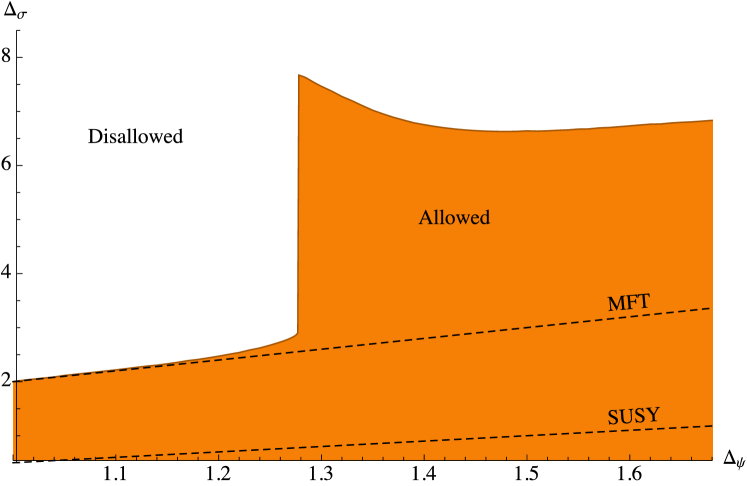
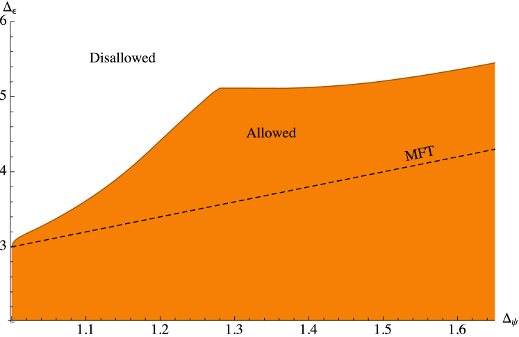
(a) (b)

Figure 28: (Color online) Upper bounds on the dimension of (a) the first parity-odd scalar $\sigma$ and (b) the first parity-even scalar $\epsilon$ in the OPE $\psi\times\psi$, as a function of $\Delta_{\psi}$ Iliesiu et al. (2016a). Here $\psi$ is a Majorana fermion primary operator in a 3d parity-invariant unitary CFT.

In Fig. 29 we also show the general lower bounds on the central charge $C_{T}$ (normalized to its value in the theory of a free Majorana fermion), obtained by bounding the coefficient of the stress-tensor conformal block. These lower bounds approach the free values as $\Delta_{\psi}\rightarrow 1$ and disappear completely for $\Delta_{\psi}\gtrsim 1.47$. In the case of $O(N)$ symmetry they can be seen to grow linearly with $N$ and are compatible with values computed in the $1/N$ expansion of the GNY model. Generalizations to the current central charge $C_{J}$ for fermions charged under $O(N)$ symmetry were also computed in Iliesiu et al. (2018b).

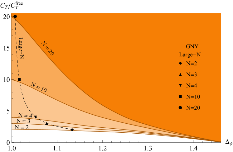
(a) (b)

Figure 29: (Color online) Lower bounds on $C_{T}$ as a function of $\Delta_{\psi}$, where $\psi$ is (a) Majorana fermion or (b) a multiplet of Majorana fermions in the fundamental representation of an $O(N)$ global symmetry group Iliesiu et al. (2016a, 2018b).

V.4.3 Gross-Neveu-Yukawa models

In the critical GNY model at large $N$, $\psi_{i}$ has dimension $1+4/(3\pi^{2}N)+\ldots$, while the leading parity-odd scalars in the $\psi_{i}\times\psi_{j}$ OPE are the $O(N)$ singlet $\phi$ with dimension $1-32/(3\pi^{2}N)+\ldots$ and the $O(N)$ symmetric tensor $\bar{\psi}_{i}\psi_{j}$ with dimension $2+32/(3\pi^{2}N)+\ldots$ (Iliesiu et al., 2018b, Table 1). The accumulation point $(\Delta_{\psi},\Delta_{\sigma})\rightarrow(1,1)$ sits well in the interior of Fig. 28(a), but by imposing a gap until the second parity-odd scalar, $\Delta_{\sigma^{\prime}}\geqslant 2+\delta$ for different positive values of $\delta$, we have the possibility of obtaining an allowed region that rules out critical GNY models with $N$ sufficiently large.

This is realized in Fig. 30, where the effect of gaps ranging from $\Delta_{\sigma^{\prime}}\geqslant 2.01$ to $\Delta_{\sigma^{\prime}}\geqslant 2.9$ are shown. At very small values of $\delta$ the lower bounds of the allowed regions possess a kink whose location matches very well to the large-$N$ GNY model prediction. At larger values of $\delta$, the precise map between $\delta$ and $N$ is not known but it is plausible that the kinks continue to match to the GNY model even at small values of $N$. However, starting around $\Delta_{\sigma^{\prime}}\geqslant 2.3$, a second lower feature also appears in these curves, where they all intersect and have an additional kink at a point near $(1.08,.565)$.

This structure of an “upper” and “lower” kink can be seen clearly in Fig. 31, specialized to the case $\Delta_{\sigma^{\prime}}\geqslant 3$. In fact, in this case the line $\Delta_{\psi}=\Delta_{\sigma}+1/2$ expected for theories with supersymmetry comes very close to (but just misses) the upper kink. Thus, it is tempting to conjecture that the $\mathcal{N}=1$ supersymmetric Gross-Neveu-Yukawa model, see Sec. V.4.1, may sit in this feature and has $\Delta_{\sigma^{\prime}}$ slightly smaller than 3. This picture seems consistent with estimate $\Delta_{\sigma}\approx 0.59$ from a Padé-extrapolation of the $\epsilon$-expansion Fei et al. (2016), as well as with the rigorous lower bound $\Delta_{\sigma}\geqslant 0.565$ Bashkirov (2013), which follows using another supersymmetric relation $\Delta_{\epsilon}=\Delta_{\sigma}+1$ together with the bootstrap bound in Fig. 7, applicable with parity playing the role of a $\mathbb{Z}_{2}$ symmetry. An additional speculation is that the lower feature may coincide with a non-supersymmetric fixed point, called GNY^∗ in Iliesiu et al. (2018b), which is seen in the $\epsilon$-expansion as a nonunitary fixed point at large $N$, but whose fate at small $N$ and $\epsilon\rightarrow 1$ is not known.

Additional evidence for this picture comes from the generalization of the bounds to $O(N)$ symmetry Iliesiu et al. (2018b), where one can place independent bounds on different $O(N)$ representations. In Fig. 32 we show computed bounds on the leading singlet dimension $\Delta_{\sigma}$, assuming that the next singlet is irrelevant, $\Delta_{\sigma^{\prime}}\geqslant 3$. These bounds also show both an upper and lower kink, which appear not too far from the $\epsilon$-expansion estimates for the GNY and GNY^∗ models. In Fig. 33 we also highlight the bounds on the leading $O(N)$ symmetric tensor $\sigma_{T}$, which display mysterious and unexplained jumps when $\Delta_{\sigma_{T}}$ reaches marginality and at smaller values of $\Delta_{\psi_{i}}$ show a series of kinks which match to the large-$N$ GNY models. Understanding the mechanism behind these jumps is an important open problem, which may be related to the spectrum rearrangement phenomena from Sec. V.2.3.

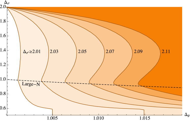
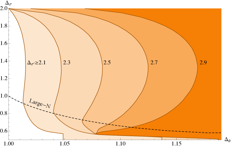
Figure 30: (Color online) Effect of imposing a gap until the second pseudoscalar $\sigma^{\prime}$ on the parameter space of 3d parity-invariant CFTs Iliesiu et al. (2016a).

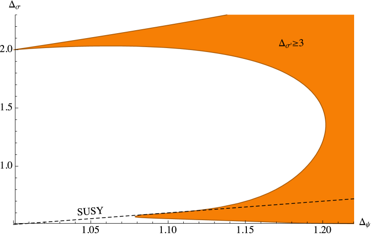
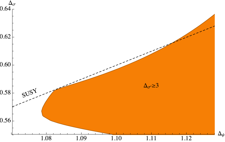
Figure 31: (Color online) Effect of imposing that there is only one relevant pseudoscalar, $\Delta_{\sigma^{\prime}}\geqslant 3$, in 3d parity-invariant CFTs Iliesiu et al. (2016a).

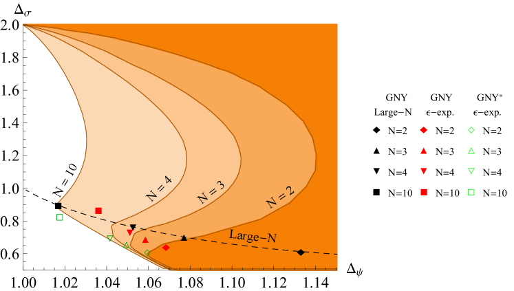
Figure 32: (Color online) Effect of imposing a gap $\Delta_{\sigma^{\prime}}\geqslant 3$ in the singlet pseudoscalar sector of $O(N)$-symmetric fermionic CFTs Iliesiu et al. (2018b). The kinks at low $N$ may perhaps be identified with the GNY and GNY^∗ CFTs.

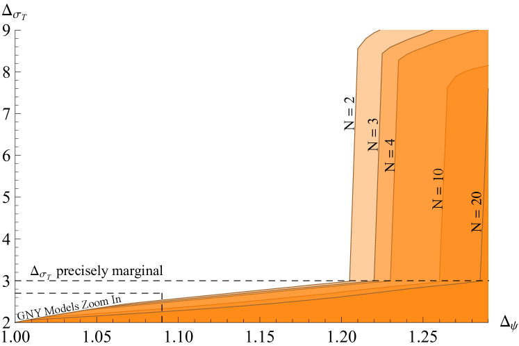
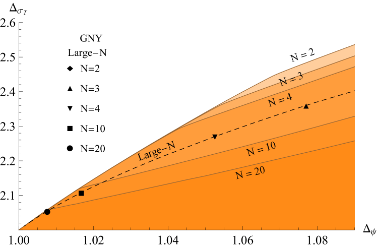
(a) (b)

Figure 33: (Color online) Upper bounds on the dimension of the symmetric traceless pseudoscalar $\sigma_{T}$ in the OPE $\psi_{i}\times\psi_{j}$ in $O(N)$-symmetric fermionic CFTs Iliesiu et al. (2018b). Notice the mysterious jumps in the wide view of the bounds (a) when they cross marginality. (b) gives a zoom on the small $\Delta_{\psi}$ region, where the bounds exhibit kinks, in agreement with the GNY dimensions at large $N$.

V.5 QED₃

Continuing our survey of physically important 3d CFTs, another class of theories are those defined by coupling 3d gauge or Chern-Simons fields to matter. One of the simplest examples is 3d quantum electrodynamics (QED₃), containing a $U(1)$ gauge field coupled to $N_{f}$ 2-component massless Dirac fermions $\psi_{i}$. This theory is known to flow to a nontrivial CFT at large $N_{f}$, which can be studied in the $1/N_{f}$ expansion Appelquist et al. (1988); Nash (1989). There has been a longstanding question of whether there is a critical value of $N_{f}$ below which the theory undergoes spontaneous breaking of the $SU(N_{f})$ global symmetry. Numerous estimates of the critical value of $N_{f}$ have been made over the years, see e.g. (Gukov, 2017, Table 5).

It would be very interesting to shed light on these theories and the question of the conformal window using bootstrap techniques. One starting point would be to study the bootstrap for 4pt functions of the gauge-invariant fermion bilinears $\bar{\psi}_{i}\psi_{j}$. Basic bootstrap bounds on scalar 4pt functions, of the type discussed in Secs. V.2, V.3, would apply to this operator, but it is not a priori clear how to isolate QED₃ as compared to other theories with similar scalar operators such as QCD₃. However, this is an under-explored direction and in future studies it may be useful to combine the bootstrap for $SU(N_{f})$ adjoints and singlets with additional gap assumptions and bootstrap constraints for other operators.

V.5.1 Monopole bootstrap for QED₃

An alternate approach, pursued in Chester and Pufu (2016) and Chester et al. (2017), is to focus on monopole operators. When dealing with a compact $U(1)$ gauge field, these operators create topologically nontrivial configurations of the gauge field having magnetic flux emerging from a spacetime point. Such operators are charged under a topological $U(1)_{T}$ global symmetry with symmetry current $J_{T}^{\mu}=\frac{1}{8\pi}\epsilon^{\mu\nu\rho}F_{\nu\rho}$. Taking the monopole operators to have charge $q\in\mathbb{Z}/2$, the scalar monopoles transform in representations of $SU(N_{f})$ corresponding to fully rectangular Young diagrams with $N_{f}/2$ rows and $2|q|$ columns Dyer et al. (2013). Thus, the lightest scalar monopoles $M^{I}_{\pm 1/2}$ are expected to be in $SU(N_{f})$ representations with $N_{f}/2$ fully antisymmetric indices.

The bootstrap for 4pt functions of $M^{I}_{\pm 1/2}$ was studied in Chester and Pufu (2016) for $N_{f}=2,4,6$, where they focused on placing bounds on the dimension of the second monopole operator $\Delta_{M_{1}}$, making various assumptions about gaps in the uncharged $(q=0)$ sector. These bounds are shown in Figs. 34, 35, where for $N_{f}=4,6$ they can be compared with the large $N_{f}$ estimate (black cross). Intriguingly, there is a kink-like discontinuity in the bound which comes close to the large $N_{f}$ estimate for certain values of the gap in the uncharged sector for operators in the same $SU(N_{f})$ representation. By increasing the gap above $M_{1}$, the allowed region could also be turned into a peninsula around the kink. Similar bounds for the lightest spinning monopoles in the case $N_{f}=4$, along with a comparison to the large $N_{f}$ predictions, were presented in Chester et al. (2017).

While these results are not definitive, they seem promising and show that the bootstrap for QED₃ has a reasonable chance to be successful, perhaps after a few more ingredients are added. Some possible directions would be to consider a multiple correlator bootstrap involving $M_{\pm 1/2}$, $M_{\pm 1}$, and/or $\bar{\psi}_{i}\psi^{j}$. It may also be fruitful to combine these with constraints from 4pt functions containing the $U(1)_{T}$ current, the $SU(N_{f})$ current, or the stress tensor.

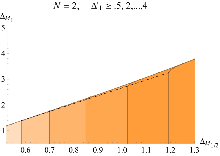
(a) (b)

Figure 34: (Color online) Bounds on $\Delta_{M_{1}}$ in terms of $\Delta_{M_{1/2}}$ in $d=3$ for $N_{f}=2,6$ (a,b) with various assumptions on the gaps in the uncharged sector in the same $SU(N_{f})$ representation as $M_{1}$ Chester and Pufu (2016).

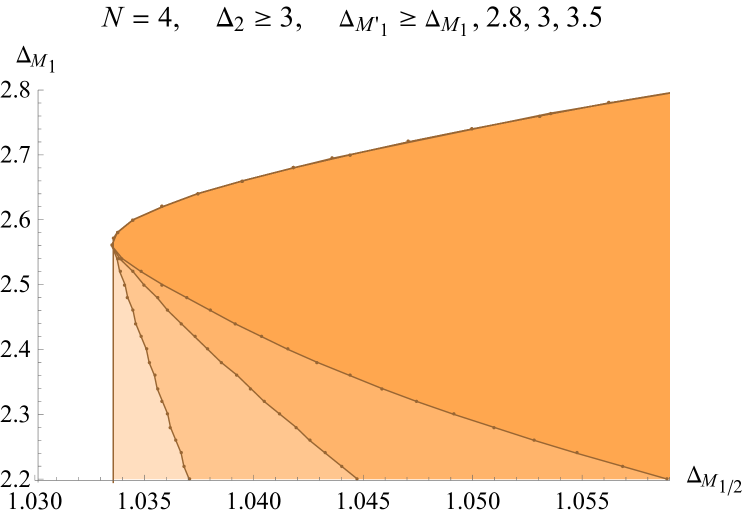
(a) (b)

Figure 35: (Color online) (a) is the analogue of Fig. 34 for $N_{f}=4$. (b) starts from the $\Delta_{2}\geqslant 3$ case of (a), and shows that placing an additional gap $\Delta_{M^{\prime}_{1}}$ above $\Delta_{M_{1}}$ turns the kink into a peninsula Chester and Pufu (2016).

V.5.2 Bosonic QED₃ and deconfined quantum critical points

Finally we would like to review the rich physics of bosonic QED₃, where some bootstrap insights have recently been obtained. Bosonic QED₃ is obtained by coupling the $U(1)$ gauge field to $N$ complex scalars $\phi_{i}$ with an $SU(N)$ invariant potential $m^{2}|\phi|^{2}+\lambda(|\phi|^{2})^{2}$. This is also known as the $N$-component abelian Higgs model, and is believed to flow to a CFT for large enough $N$. Unlike for fermions, the boson mass term preserves all the symmetries and has to be fine-tuned to reach the fixed point.

This model has been much discussed in the condensed matter literature as the “non-compact CP^N-1 model” (NCCP^N-1) in connection with the phenomenon of “deconfined criticality” Senthil et al. (2004). To briefly review this connection, the physical systems of interest are certain quantum antiferromagnets in $(2+1)$ dimensions, which have a quantum phase transition between Néel and Valence-Bond-Solid (VBS) phases. The transition can be described by the $O(3)$ nonlinear sigma model (NLSM) for the Néel order parameter, modified by the inclusion of Berry phase effects which suppress topological defects (hedgehogs), which will play an important role below.

The $O(3)$ NLSM can be written as the CP¹ model, which has two complex vectors $\mathbf{z}=(z_{1},z_{2})$ subject to the constraint $|z_{1}|^{2}+|z_{2}|^{2}=1$ and a $U(1)$ gauge invariance $\mathbf{z}\sim e^{i\phi}\mathbf{z}$. This explains the emergence of the gauge field. Replacing the constraint by a quartic potential, and adding a Maxwell kinetic term for the gauge field (expected to be generated by the RG flow), one obtains bosonic QED₃ with $N=2$.

In the language of QED₃, the above-mentioned topological defects are the monopole operators of quantized charge, similar to the ones in Sec. V.5.1. Of course the dimensions of monopole operators differ in bosonic and fermionic QED. Also here we will normalize the topological charge to be integer $q\in\mathbb{Z}$.

If a monopole of charge $q$ appears in the action, it breaks the global topological $U(1)_{T}$ symmetry to the $\mathbb{Z}_{q}$ subgroup. Microscopic descriptions of quantum antiferromagnets may realize a discrete subgroup of $U(1)_{T}$ at the lattice level. On cubic lattices, a $\mathbb{Z}_{q_{0}}$ with $q_{0}=4$ is preserved, while for the hexagonal and rectangular lattices we have $q_{0}=3$ and $q_{0}=2$. The $\mathbb{Z}_{q_{0}}$ symmetry is also visible in the VBS phase where it permutes the vacua. This microscopic symmetry means that only monopoles with charges multiple of $q_{0}$ appear. Monopoles with different charges have their fugacity killed by the above-mentioned Berry phases Read and Sachdev (1990).

In light of the above discussion, the analysis of the critical behavior of QED₃ can be split into two parts. First, does bosonic QED₃, with all monopoles suppressed, have a fixed point? If the answer is yes, then one can ask: can this fixed point be reached provided that one allows monopoles with charges in multiples of $q_{0}$? For this to happen, the monopole of charge $q_{0}$ has to be irrelevant.

One can study these questions analytically at large $N$: one finds a fixed point and computes the critical exponents in the $1/N$ expansion. At small $N$ one resorts to Monte Carlo simulations. The bootstrap at present cannot by itself resolve the question of the fixed point existence. However, it can provide valuable consistency checks on the other studies. Suppose that a certain Monte Carlo simulation is done on a lattice preserving a $\mathbb{Z}_{q_{0}}$ subgroup, finds a second order phase transition, and measures the scaling dimensions $\Delta_{q}$ of monopole operators $M_{q}$ for a subset of charges $q$ (we denote by $M_{0}$ the relevant singlet scalar driving the transition). We have the following OPE algebra in the scalar sector, omitting the OPE coefficients ($M_{-q}=M_{q}^{\dagger}$):

$$M_{q}\times M_{q^{\prime}}\sim\delta_{q+q^{\prime}}\mathds{1}+M_{q+q^{\prime}}+\ldots\,.$$ (126)

By the above discussion, the operator $M_{q_{0}}$ has to be irrelevant, as well as the higher charge monopoles. We can use the bootstrap to study the consistency of this algebra given the measured operator dimensions.

V.5.3 Aside: constraints on symmetry enhancement

What we just presented is an instance of a more general question: under which conditions can the global symmetry of the fixed point $G$ be larger than the microscopically realized symmetry $H$? The case of interest for the previous section is $G=U(1)$ and $H=\mathbb{Z}_{q_{0}}$. For the symmetry enhancement to happen, operators which break $G$ to $H$ must be irrelevant. The bootstrap is a powerful tool to study whether this irrelevance assumption is consistent with conformal symmetry and with other information which may be available about the fixed point. We will see further applications of this philosophy in Secs. VI.2 and VI.3.

We will now describe bootstrap constraints on the symmetry enhancement from $\mathbb{Z}_{q_{0}}$ to $U(1)$ derived by Nakayama and Ohtsuki (2016). Enhancement from $\mathbb{Z}_{2}$ requires that $M_{2}$ is irrelevant. Since $M_{1}\times M_{1}\sim M_{2}$, one can bound $\Delta_{2}$ given $\Delta_{1}$, by studying the 4pt function $\langle M_{1}M_{1}^{\dagger}M_{1}M_{1}^{\dagger}\rangle$. The resulting bound is given in Fig. 36. Imposing $\Delta_{2}>3$, one gets a necessary condition $\Delta_{1}>1.08$ for enhancement from $\mathbb{Z}_{2}$ to $U(1)$.

Figure 36: (Color online) The 3d upper bound on $\Delta_{2}$ as a function of $\Delta_{1}$ Nakayama and Ohtsuki (2016). It may be possible to improve this bound if $\Delta_{0}$ is known. The same bound applies to $M_{2}\times M_{2}\sim M_{4}$.

The same plot in Fig. 36 can be used to derive rough necessary conditions on the enhancement from $\mathbb{Z}_{4}$ to $U(1)$. Indeed, the bound applies also to $M_{2}\times M_{2}\sim M_{4}$. If $M_{4}$ is irrelevant, then we must have $\Delta_{2}>1.08$, which in turn implies $\Delta_{1}>0.504$.

To study enhancement from $\mathbb{Z}_{3}$, one analyzes simultaneously three 4pt functions $\langle M_{1}M_{1}^{\dagger}M_{1}M_{1}^{\dagger}\rangle$, $\langle M_{1}M_{1}^{\dagger}M_{2}M_{2}^{\dagger}\rangle$, $\langle M_{2}M_{2}^{\dagger}M_{2}M_{2}^{\dagger}\rangle$. It is reasonable to assume that $M_{4}$ is irrelevant (as would be the case if $M_{3}$ is irrelevant and $\Delta_{q}$ is monotonic in $q$), and to impose $\Delta_{0}>1.044$ (which follows from an assumption that the fixed point is critical and not multicritical, see Sec. V.1). Under these assumptions, the upper bound on $\Delta_{3}$ as a function of $\{\Delta_{1},\Delta_{2}\}$ is shown in Fig. 37. From this bound, irrelevance of $M_{3}$ requires $\Delta_{1}>0.585$.

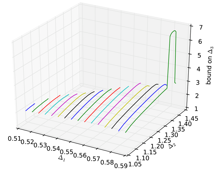
Figure 37: (Color online) An upper bound on $\Delta_{3}$ as a function of $\{\Delta_{1},\Delta_{2}\}$ under the assumptions that $\Delta_{0}>1.044$, $\Delta_{4}>3$ Nakayama and Ohtsuki (2016). It follows from Fig. 36 that the range of $\Delta_{2}$ is restricted by the latter assumption from below, and, for fixed $\Delta_{1}$, from above.

V.5.4 Back to deconfined criticality: is the transition second order?

The necessary conditions described in the previous section have been compared with available Monte Carlo and large $N$ data on the Néel-VBS transition which claim to see a second-order transition and measure some critical exponents. For square and hexagonal lattices, there is nice consistency, as for rectangular lattices for $N\leqslant 4$ and $N\geqslant 6$, while some $N=5$ simulations are inconsistent with the bootstrap. The conclusion is that there must either be an error in the $N=5$ Monte-Carlo measurement or in the assumption that the transition is second-order. See Nakayama and Ohtsuki (2016) for this survey and for further details.

It should be emphasized that while the bootstrap results may point out an inconsistency in Monte Carlo simulations, they cannot, at present, validate them and prove that the phase transition is indeed second order. It is still possible that even in the above cases when there is a nice agreement between Monte Carlo results and the bootstrap necessary conditions, the transition is still very weakly first order and not second order.

Let us focus on the case $N=2$ which presents a controversy. Large-scale Monte Carlo simulations for $N=2$ were performed in Nahum et al. (2015a), using a loop model on a cubic lattice which is in the same universality class as NCCP¹ and has monopole suppression up to $q_{0}=4$, and going up to very large lattices of linear size up to $L=640$. While they have not seen signs of a finite correlation length or a conventional first order transition, and observed scaling behavior of correlation functions at distances $1\ll r\ll L$, they have seen scaling violation for observables at larger distances $r\sim L$, inconsistent with a conventional second order transition.

So, is the transition second order or weakly first order? Assuming a second order transition, Nahum et al. (2015a) extracted the scaling dimension of the monopole operator $\Delta_{1}=0.625(15)$, which is consistent with the bootstrap condition $\Delta_{1}>0.504$ necessary for the enhancement from $\mathbb{Z}_{4}$ to $U(1)$. However there is an extra piece of information which allows one to set up an even more stringent bootstrap test: further symmetry enhancement at the transition from $SO(3)\times U(1)$ to $SO(5)$. Here $SO(3)$ acts on the Néel order parameter $N_{a}=\mathbf{z}^{\dagger}\sigma_{a}\mathbf{z}$. Empirically, the scaling dimension of $N$ is very close to $\Delta_{1}$ Nahum et al. (2015a) and, moreover, the joint probability distribution of $(N,M_{1})$ is very close to the spherical one after a rescaling Nahum et al. (2015b), which can be explained if $N$ and $M_{1}$ belong to a vector multiplet $\Phi$ of $SO(5)$ of dimension $\Delta_{\Phi}=\Delta_{1}$.

In this description, the relevant scalar which drives the transition is a component of the symmetric traceless tensor (roughly $\Phi_{A}\Phi_{B}-\text{trace}$). For the $SO(5)$ enhancement to happen, any other scalar which breaks $SO(5)$ back to $SO(3)\times U(1)$ must be irrelevant. In addition, the $SO(5)$ singlet $S$ (roughly $\Phi_{A}\Phi^{A}$) must be irrelevant for the transition to be second order, since otherwise the fixed point will not be reached. See Wang et al. (2017) for further discussion. Given the dimension $\Delta_{\Phi}=\Delta_{1}$ as above, it is straightforward to compute an upper bound on the dimension of $S$ which occurs in the OPE $\Phi\times\Phi$. This is the same bound as for $N=5$ in Fig. 21 except the plot has to be extended to larger $\Delta_{\Phi}$. Nakayama and Ohtsuki (2016) and Simmons-Duffin (2016b) performed this analysis and report that $\Delta_{S}>3$ is excluded for $\Delta_{\Phi}$ as above. In fact $\Delta_{S}>3$ requires $\Delta_{\Phi}>0.76$ Nakayama (2016a).

To summarize, the bootstrap excludes a second-order phase transition described by a unitary 3d CFT with symmetry enhanced to $SO(5)$ and the order parameter scaling dimension taking the above value suggested by the Monte Carlo simulations. In our opinion, the most compelling interpretation of available data is a weakly first-order transition due to walking RG behavior which ensues when the RG flow has no fixed points for a real value of the coupling but two complex conjugate fixed points with small imaginary parts. This is the same mechanism as for the weakly first-order transition in the 2d Potts model with $Q\gtrsim 4$. As discussed in Nahum et al. (2015a), this scenario may resolve the observed scaling violations at distances $r\sim L$. It can also accommodate the enhancement to $SO(5)$ Wang et al. (2017). In this scenario, there is no unitary 3d CFT (the complex fixed points being nonunitary), and the bootstrap bounds do not apply, resolving the contradiction.

Finally, let us note that a similar analysis can constrain another scenario outlined in Wang et al. (2017), in which a variant called the easy-plane NCCP¹ model is conjectured to have a fixed point with enhanced $O(4)$ symmetry and be dual to $N_{f}=2$ fermionic QED₃. In this scenario, the conjectured fixed point cannot contain any fully $O(4)$-invariant scalar perturbations. However, recent Monte Carlo simulations Qin et al. (2017) point to a dimension for the $O(4)$ vector order parameter $\Delta_{\Phi}=0.565(15)$ which seems incompatible with the bootstrap bound assuming irrelevance of the $O(4)$ singlet (Fig. 20 extended further to the right), which requires $\Delta_{\Phi}>0.868$ Poland (2017). In the future it will be interesting to further study the fate of these models using both bootstrap and Monte Carlo data.

V.6 Current and stress-tensor bootstrap

In the previous sections we discussed results following from 4pt functions of scalars and fermions. Here we wish to discuss interesting results which have recently been obtained from 4pt functions of tensor operators, specifically of conserved currents and stress tensors. Namely, a number of numerical bounds on scaling dimensions and OPE coefficients from such correlators in parity-preserving 3d CFTs were recently computed in Dymarsky et al. (2017) and Dymarsky et al. (2018), building on important analytical developments for spinning correlators, as reviewed in Sec. III.6.7. Such studies are well-motivated because they probe the general space of local CFTs, and may even lead to the discovery of new theories.

A concrete application of these constraints is to study bounds on current and stress-tensor 3pt function coefficients under various assumptions. These coefficients are known to satisfy various analytical bounds following from the averaged null energy condition (see Sec. III.5.3), as was originally argued in the context of conformal collider physics in Hofman and Maldacena (2008), with 3d bounds worked out in Buchel et al. (2010); Chowdhury et al. (2013). One application of the numerical bootstrap is to study how the conformal collider bounds change as a function of gaps. Another application is to determine these coefficients in various CFTs, e.g. the critical 3d Ising and $O(N)$ models. These studies also allow one to probe parity-odd operators in the spectrum which have previously been inaccessible from the perspective of scalar 4pt functions (although they could be accessed from the fermionic correlators in Sec. V.4).

In Fig. 38 we show general lower bounds on the central charge (in units of the free boson central charge $C_{B}$) from the bootstrap applied to $\langle TTTT\rangle$, as a function of the independent parity-preserving $\langle TTT\rangle$ 3pt function coefficient which is parametrized by the variable $\theta$. In this notation the conformal collider bound is $0\leqslant\theta\leqslant\pi/2$, where a free scalar has $\theta=0$ and free Majorana fermion has $\theta=\pi/2$. It can be readily seen that the numerical bootstrap is able to reproduce this constraint in addition to giving general lower bounds on $C_{T}$. A similar set of bounds from the $\langle JJJJ\rangle$ bootstrap is shown in Fig. 39, where in this plot $C_{T}$ is normalized to the central charge of a free complex scalar $C_{T}^{\text{free}}$ and the independent parity-preserving $\langle JJT\rangle$ coupling is parametrized by $\gamma$, where the conformal collider bound is given by $-\frac{1}{12}\leqslant\gamma\leqslant\frac{1}{12}$. In this case the free complex scalar has $\gamma=-\frac{1}{12}$ while the free Dirac fermion has $\gamma=\frac{1}{12}$.

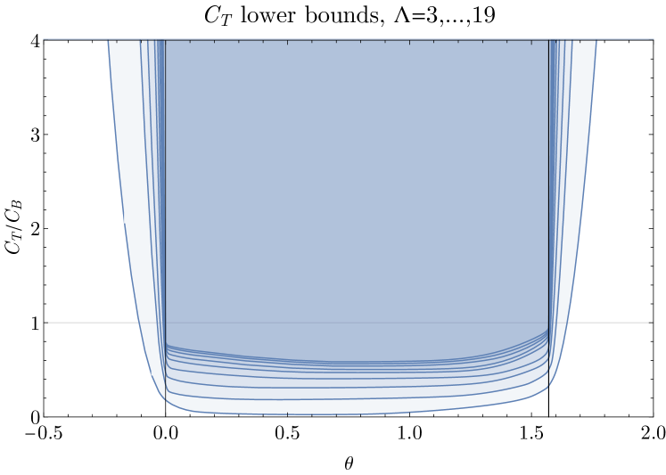
Figure 38: (Color online) Bounds on $C_{T}$ as a function of the $\langle TTT\rangle$ 3pt function parameter $\theta$ Dymarsky et al. (2018).

Figure 39: (Color online) Bounds on $C_{T}$ as a function of the $\langle JJT\rangle$ 3pt function parameter $\gamma$ Dymarsky et al. (2017).

As mentioned above, the advantage of the numerical bootstrap is that it can readily probe how constraints on these couplings depend on gaps in the spectrum. For example, in Fig. 40 we show how the lower bound on $C_{T}$ as a function of $\theta$ in the $\langle TTTT\rangle$ bootstrap varies as one increases the gap in the parity-odd scalar sector $\Delta_{\text{odd}}$ from $2$ to $8$. It can be seen that increasing the parity-odd gap forbids the “fermion” end of the range for $\theta$ but allows the “scalar” end. This is consistent with the fact that the free scalar has a very large parity odd gap $\Delta_{\text{odd}}=11$, while the free Majorana fermion has a small gap $\Delta_{\text{odd}}=2$.

Similarly, imposing a parity-even gap forbids the “scalar” end. In Fig. 41 we illustrate this by showing what happens when the leading parity-even scalar is irrelevant, corresponding to “self-organized” CFTs (see Sec. V.1). This lower central charge bound applies for instance to fermionic QED₃ in the conformal window from Sec. V.5, with $N_{f}$ even for parity invariance.

Furthermore, imposing gaps on both parity-even and parity-odd scalars forces one to live with intermediate values of $\theta$, at least for moderately small values of the central charge. These and other bounds with different gap assumptions (including upper bounds on $C_{T}$ for gaps excluding large-$N$ theories) can be found in Dymarsky et al. (2018).

A similar story holds for bounds from the $\langle JJJJ\rangle$ bootstrap, where Fig. 42 shows how the lower bound on $C_{T}$ changes when either parity-even or parity-odd scalars are irrelevant (dashed blue lines), or when both are irrelevant (solid blue line). These bounds are consistent with the gaps for a free complex scalar ($\Delta_{0}^{+}=2$, $\Delta_{0}^{-}=7$) and free Dirac fermion ($\Delta_{0}^{+}=4$, $\Delta_{0}^{-}=2$). Similar bounds with different gap assumptions can be found in Dymarsky et al. (2017). In the future, by generalizing this analysis to $SU(N_{f})$ (or $SU(N_{f})\times U(1)$) global symmetry one may be able to place interesting bounds on the fermionic QED₃ central charge using the same argument as the one based on Fig. 41.

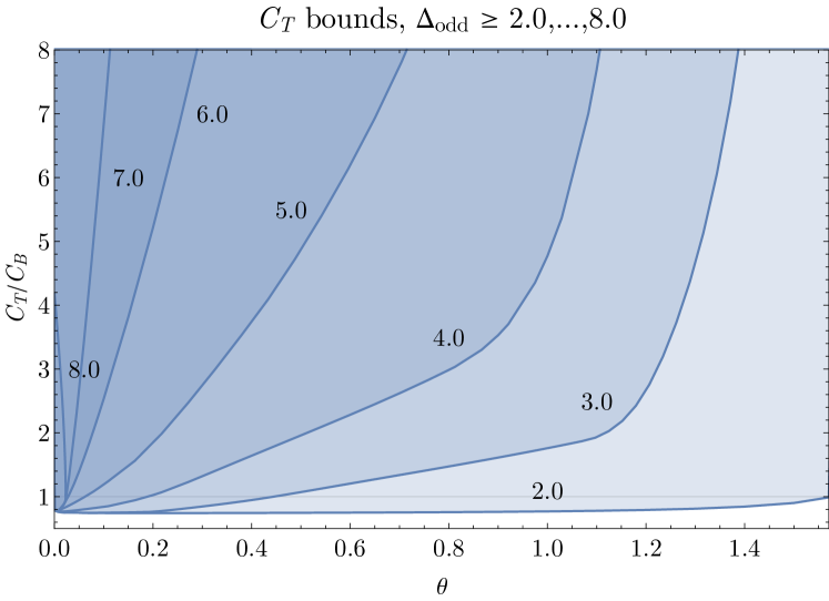
Figure 40: (Color online) Bounds on $C_{T}$ as a function of the $\langle TTT\rangle$ 3pt function parameter $\theta$ for different values of the parity-odd scalar gap $\Delta_{\text{odd}}$ Dymarsky et al. (2018).

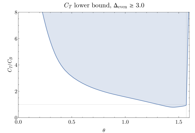
Figure 41: (Color online) Bounds on $C_{T}$ as a function of the $\langle TTT\rangle$ 3pt function parameter $\theta$ assuming that the leading parity-even scalar is irrelevant Dymarsky et al. (2018).

It is interesting to ask if one can use these general bootstrap constraints to determine $\theta$ or $\gamma$ in some CFTs of interest, e.g. the Ising or $O(2)$ models. In the case of the Ising model, it is a plausible assumption (e.g., from the $\epsilon$-expansion) that its leading parity-odd (but $\mathbb{Z}_{2}$-even) operator has a very large dimension as in the free scalar theory. Using known parity-even data the $\langle TTTT\rangle$ bootstrap yields an upper bound $\Delta^{\text{Ising}}_{\text{odd}}<11.2$, and one can obtain small closed regions in the $\{\theta,C_{T}\}$ plane that are consistent with the known Ising central charge, Eq. (123). These regions, shown in Fig. 43, yield the determination $0.01<\theta<0.018-0.019$ if $\Delta_{\text{odd}}$ is close to saturating its bound. Note that if one makes the weaker assumption of irrelevance $\Delta_{\text{odd}}>3$, then there is still a reasonably tight range $0.01<\theta<0.05$ consistent with $C_{T}^{\text{Ising}}$.

In the case of the $\langle JJJJ\rangle$ bootstrap, one can similarly try to determine $\gamma$ for the $O(2)$ model. In this case after inputting the known dimension of the leading $O(2)$ parity-even singlet, irrelevance of the second $O(2)$ parity-even singlet, and the plausible parity-odd gaps $\Delta_{0}^{-}\geqslant 5$ and $\Delta_{\ell}^{-}\geqslant\ell+2$, Fig. 44 yields the range $-0.0824<\gamma<-0.0494$. Based on a linear extrapolation, Dymarsky et al. (2017) also estimated the more restrictive range $-0.080<\gamma<-0.061$. A negative value of $\gamma$ in the $O(2)$ model also appears to be favored by the results of quantum Monte Carlo simulations Katz et al. (2014). In future work it will be interesting to find ways to improve these determinations, extend them to other $O(N)$ models, and perhaps connect the smallness of the deviations of $\theta$ and $\gamma$ from their free values to the existence of approximate higher-spin currents in these theories.

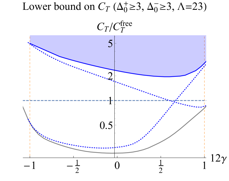
Figure 42: (Color online) Bounds on $C_{T}$ as a function of the $\langle JJT\rangle$ 3pt function parameter $\gamma$ with no assumptions (lower solid curve), parity-odd scalars irrelevant (lower dashed curve), parity-even scalars irrelevant (upper dashed curve), and all scalars irrelevant (upper solid curve) Dymarsky et al. (2017).

Figure 43: (Color online) Bounds on $C_{T}$ as a function of the $\langle TTT\rangle$ 3pt function parameter $\theta$ with gap assumptions plausible for the Ising model Dymarsky et al. (2018).

Figure 44: (Color online) Bounds on $C_{T}$ as a function of the $\langle JJT\rangle$ 3pt function parameter $\gamma$ with gap assumptions plausible for the critical $O(2)$ model Dymarsky et al. (2017).

Finally, in Fig. 45 we show a more global picture of the allowed region of parity-odd and parity-even scalar gaps from both the $\langle TTTT\rangle$ and $\langle JJJJ\rangle$ bootstrap, making no additional assumptions. These regions satisfy a number of consistency checks, e.g. being consistent with known gaps in free theories, MFTs, and critical $O(N)$ models. They additionally show fairly sharp features near the scaling dimensions in the Ising and $O(2)$ models. It will be interesting to improve these maps in future studies and identify the locations of other CFTs of interest. The lower “scalar exclusion” regions of these plots are ruled out from 4pt functions of the leading parity-odd scalar (assuming the parity-even scalar appears in both OPEs as would be generically expected), an example of how the scalar and the stress-tensor/current bootstraps can yield complementary information.

(a) (b)

Figure 45: (Color online) Allowed region for parity-even and parity-odd scalar gaps from (a) $\langle TTTT\rangle$ bootstrap Dymarsky et al. (2018) and (b) $\langle JJJJ\rangle$ bootstrap Dymarsky et al. (2017).

There are a number of directions for future work, which include considering mixed systems containing stress tensors/currents together with scalars, studying the implications of parity violation (see footnote 129), studying in more detail the conditions for large $N$ and holographic theories, and generalizing these studies to other dimensions. Recent progress on how to compute spinning conformal blocks in 4d and in general dimensions should make these analyses tractable in the future outside of 3d. Current and stress-tensor multiplets can also be considered in superconformal theories, where the bootstrap analysis can be simplified using the fact that they reside in multiplets with operators of lower spin.

V.7 Future targets

In this section we will collect some additional 3d models which in our opinion represent interesting future targets for the bootstrap.

V.7.1 Multifield Landau-Ginzburg models

There exists rich phenomenology of fixed points arising from Lagrangians with multiple scalar fields transforming under product group symmetries, e.g. $SO(n)\times SO(m)$. One can consider Lagrangians involving two coupled scalar multiplets, one transforming in the fundamental of $SO(n)$ and another of $SO(m)$. Alternatively, one can consider a field transforming in the bifundamental of $SO(n)\times SO(m)$. Such Lagrangians have been invoked to describe phase transitions in many physical systems; see Vicari (2007) for further details.

When studying these fixed points using the RG, a recurrent feature is that many of them do not exist in the $4-\epsilon$ expansion and have to be studied directly in 3d. Since such computations lack a manifestly small expansion parameter, there seems to be no consensus about the existence of these fixed points. So this appears to be a perfect target for a nonperturbative approach like the bootstrap. Some preliminary bootstrap studies of 3d CFTs with $SO(n)\times SO(m)$ were carried out in Nakayama and Ohtsuki (2014a, 2015), but in our opinion more work is needed before firm conclusions can be drawn.

V.7.2 Projective space models

An interesting 3d lattice model is the CPⁿ model, where microscopic lattice variables belong to CPⁿ and have ferromagnetic interactions preserving the symmetry (see below for the antiferromagnetic case). Recall that CPⁿ can be realized by starting with $(n+1)$-dimensional complex vectors $\mathbf{z}=(z_{1},\ldots,z_{n+1})$ and imposing the constraint $\mathbf{z}^{\dagger}\cdot\mathbf{z}=1$, preserved up to the equivalence $\mathbf{z}\sim e^{i\phi}\mathbf{z}$. A simple lattice Hamiltonian is

$$H=-J\sum_{\langle ij\rangle}|\mathbf{z}^{\dagger}_{i}\cdot\mathbf{z}_{j}|^{2}\,,$$ (127)

with $J>0$ in the considered ferromagnetic case. The physics of this model is influenced by defects (hedgehogs), which are possible because $\pi_{2}(CP^{n})=\mathbb{Z}$. Here we consider the CPⁿ model with defects allowed. It should be distinguished from the “non-compact CPⁿ model” which results when defects are suppressed, see Sec. V.5.2.

The CP¹ model is equivalent to the $O(3)$ model, with the order parameter $N_{a}=\mathbf{z}^{\dagger}\sigma_{a}\mathbf{z}$, and it has a second-order phase transition described by the same CFT.

The CP² model has an internal symmetry $SU(3)$ (modulo global issues), with traceless hermitian matrix $Q_{ab}=z_{a}\bar{z}_{b}-\delta_{ab}$ as an order parameter. The Landau-Ginzburg description contains a cubic invariant ${\rm Tr}(Q^{3})$ and would suggest a first-order transition, but Monte Carlo simulations Nahum et al. (2013) indicate that the phase transition is continuous. This is similar to what happens for the 3-state Potts model in 2d and can be explained as an effect of fluctuations. Monte Carlo results for the critical exponents are $\eta=0.23(2)$ and $\nu=0.536(13)$, translating into the dimensions of $Q$ and of the relevant singlet scalar. Can this model be isolated using the numerical bootstrap?

One can also consider antiferromagnetic projective space models, taking $J<0$ in the above Hamiltonian. Antiferromagnetic CPⁿ models Delfino et al. (2015) don’t give rise to new universality classes. On the other hand, a new class is observed for the antiferromagnetic RP⁴ model Pelissetto et al. (2018), and it could constitute a target for the bootstrap.

V.7.3 Nonabelian gauge and Chern-Simons matter theories

While we have focused our attention on QED₃, there is a whole landscape of 3d gauge theories coupled to various types of matter. An interesting case is QCD₃ with a simple gauge group $G$ coupled to $N_{f}$ fundamental fermions. Such theories may for example play a role in the physics of cuprate superconductors Chowdhury and Sachdev (2015, 2014). A fixed point can be established and the properties studied at large $N_{f}$ Appelquist and Nash (1990). For example, in Dyer et al. (2013) a systematic study of monopole operators in such theories was performed, allowing for estimates of the bottom of the conformal window for different choices of $G$ by imposing irrelevance of the monopole operators (Dyer et al., 2013, Table 4). QCD₃ coupled to both fermions and scalars was also proposed to describe the critical point of the ‘orthogonal semi-metal’ (OSM) confinement transition in Gazit et al. (2018), with critical exponents extracted in quantum Monte Carlo simulations. It would be very interesting to understand how to isolate these theories using bootstrap techniques and test these estimates.

Another natural set of targets consists of Chern-Simons gauge fields coupled to matter. Such theories are known to have conformal fixed points and sit in an intricate web of dualities. Some possible experimental realizations of these theories as transitions between fractional quantum Hall states were proposed in Lee et al. (2018). A hallmark of these theories is the existence of parity-violation; it would be interesting to see if they can be found after introducing parity-violating couplings into the bootstrap. Monopole operators in these theories were also recently studied in Chester et al. (2017) and would constitute natural targets for the bootstrap.

V.7.4 Other models

Another theory briefly mentioned in Sec. V.3.4 is the Gross-Neveu-Heisenberg (GNH) model, a variant of the GN models with a 3-component scalar order parameter. For a pedagogical review of the model, its applications, and its connection to the lattice Hubbard model, see Sachdev (2010). This constitutes another interesting target for the bootstrap.

A 3d CFT with $SU(4)$ global symmetry and an order parameter in the symmetric tensor representation was considered in Basile et al. (2005, 2006). It was proposed to describe a continuous chiral phase transition in 4d $SU(N)$ gauge theory coupled to $N_{f}=2$ massless quarks in the adjoint representation at finite temperature. The existence of this CFT and some information about critical exponents was found using RG methods; it would be interesting to explore it using the bootstrap.

VI Applications in $d=4$

In this section we now turn to numerical bootstrap applications in unitary 4d CFTs. We first present general constraints in Sec. VI.1, and then discuss more specific physical applications. In Sec. VI.2 we review applications to high energy physics beyond the Standard Model. Applications to 4d conformal gauge theories will be discussed in Sec. VI.3. Supersymmetric 4d CFTs will be presented in the next section.

VI.1 General results

This section will follow the same logic as Secs. V.2.1 and V.3.1 devoted to 3d CFTs. Historically however the very first attempt to study crossing relations using numerical techniques focused on 4d CFTs. This analysis, pioneered in Rattazzi et al. (2008) and then refined in Rychkov and Vichi (2009), was spurred by high energy physics motivations which will be reviewed in Sec. VI.2. But first let us discuss general conformal bootstrap results for 4d CFTs with various global symmetries.

Consider first the simple case of a 4d CFT containing a scalar operator $\phi$ with dimension $\Delta_{\phi}$. We further assume that it is charged under a global symmetry (e.g., a $\mathbb{Z}_{2}$ symmetry) so that the OPE $\phi\times\phi$ does not contain $\phi$. Then it is interesting to ask how high can one push the dimension of the first scalar operator in this OPE. It is also interesting to ask how large the OPE coefficient of the stress tensor $\lambda_{\phi\phi T}\propto\Delta_{\phi}/\sqrt{C_{T}}$ is allowed to be Poland and Simmons-Duffin (2011); Rattazzi et al. (2011b), which translates into a lower bound on the central charge $C_{T}$. The best bounds to date were computed in Poland et al. (2012) and are shown in Fig. 46. When $\Delta_{\phi}$ approaches the unitarity bound, both bounds approach the free theory value for $\Delta_{\phi^{2}}$ and $C_{T}$. This is consistent with the fact that a scalar with dimension $(d-2)/2$ satisfies $\partial^{2}\phi=0$ whenever inserted in a correlation function, and must therefore be a free scalar.

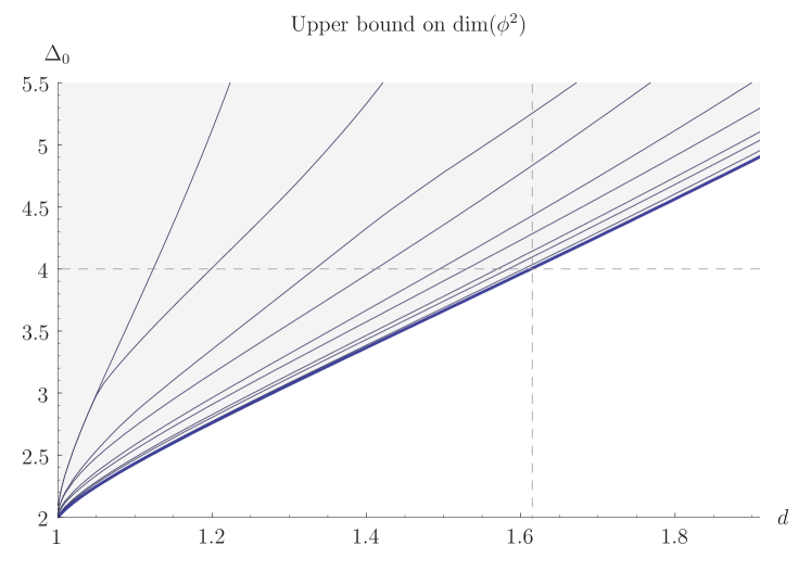
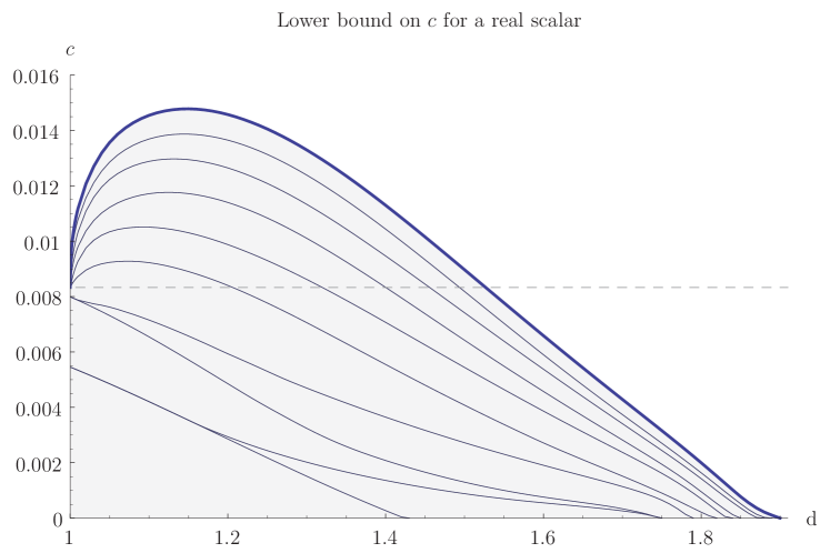
(a) (b)

Figure 46: (Color online) (a) Upper bound on the dimension of the first scalar in the $\phi\times\phi$ OPE as a function of $\Delta_{\phi}$ in 4d unitary CFTs; (b) lower bound on the central charge $C_{T}$, computed by maximizing the OPE coefficient $\lambda_{\phi\phi T}$ Poland et al. (2012).

Analogous bounds have been obtained for CFTs assuming various continuous global symmetries. Poland et al. (2012) studied the 4pt functions of a scalar $\phi$ transforming in the fundamental representation of $SO(N)$ or $SU(N)$, deriving an upper bound on the dimension of the lowest singlet scalar in the OPEs $\phi_{i}\times\phi_{j}$ (or $\phi^{\dagger i}\times\phi_{j}$ in the case of $SU(N)$), as well as a lower bound on the central charge, shown in Fig. 47. As expected, the bounds scale with $N$, the size of the fundamental representation, at least when the dimension of the external scalar approaches the free value. It should be possible to extend this analysis to obtain upper bounds on the dimensions of operators transforming in other representations. For scalars in the symmetric traceless representation of $SO(4)$ this was done in Poland et al. (2012).

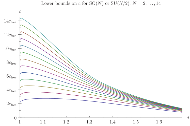
(a) (b)

Figure 47: (Color online) (a) Upper bounds on the singlet scalar dimension in $SO(N)$ and $SU(N)$ symmetric 4d CFTs, as a function of $\Delta_{\phi}$ in the fundamental; (b) lower bounds on $C_{T}$ in the same theories Poland et al. (2012).

It is also possible to place upper bounds on the OPE coefficients of conserved vectors of dimension 3 in the OPE of $\phi$ with its conjugate. This class of operators includes the conserved currents of the considered global symmetry $G=SO(N)$ or $SU(N)$, transforming in the adjoint representation of $G$. Upper bounds on their OPE coefficients translate into the lower bounds on the central charges $C_{J}$. These bounds are shown in Fig. 48. Once again the $SU(N/2)$ bounds coincide with $SO(N)$ ones Caracciolo et al. (2014). For $\Delta_{\phi}$ close to the free value, these bounds smoothly approach the free $SO(N)$ value.

In addition, for $G=SU(N)$ the OPE $\phi^{\dagger i}\times\phi_{j}$ may also contain conserved currents of some other global symmetry which may exist in the theory, which are singlets under $G$. The lower bound on their inverse-square OPE coefficient is given in Fig. 49. Close to the free theory dimension, these bounds approach the value corresponding to the theory of $N$ massless complex scalar fields, whose full symmetry $SO(2N)$ is indeed larger that $SU(N)$.

Additionally, Caracciolo et al. (2014) derived lower bounds on $C_{J}$ in the presence of a gap in the scalar singlet sector, as well as for extended global symmetries $SO(N)\times SO(M)$ and $SO(N)\times SU(M)$.

Figure 48: (Color online) Lower bound on $C_{J}$ in $SO(N)$-symmetric unitary 4d CFTs as a function of the dimension of a scalar in the fundamental Poland et al. (2012). $SU(N/2)$ adjoint currents satisfy the same bound Caracciolo et al. (2014).

Figure 49: (Color online) Lower bound on the inverse square OPE coefficient of a singlet current in $SU(N)$-symmetric unitary 4d CFTs as a function of dimension of a scalar in the fundamental Poland et al. (2012).

Unlike in 3d, most of the 4d bounds computed so far do not display any prominent kink or other dramatic feature, suggesting that existing 4d CFTs may lie inside the allowed regions and not on the boundary. Note however that some unexplained features are visible in the $C_{J}$ lower bounds in Fig. 48, as well as in the bounds on supersymmetric CFTs discussed in Sec. VII.

The bounds discussed in this section have been obtained by studying a 4pt function $\langle\phi_{i}\phi_{j}\phi_{k}\phi_{l}\rangle$ or $\langle\phi_{i}\phi^{\dagger j}\phi_{k}\phi^{\dagger l}\rangle$, where $\phi_{i}$ is a single primary operator or a global symmetry multiplet of primary operators. As far as we are aware, a systematic study of numerical bootstrap constraints from mixed correlators in 4d CFTs has not yet been performed outside of the supersymmetric context Lemos and Liendo (2016a); Li et al. (2017b). It will be important to do so in the future, and to study the impact on such bounds of assuming only a limited set of relevant operators.

VI.2 Applications to the hierarchy problem

Next we will review some bootstrap results which shed light on the attempts to alleviate the hierarchy problem of the Standard Model (SM) of particle physics, which historically was one of the motivations for the development of the numerical bootstrap in 4d.

For the purposes of our discussion, the hierarchy problem can be briefly summarized as follows. The SM is certainly not the complete description of fundamental interactions, as it doesn’t account for dark matter, baryogenesis, neutrino masses, and gravity. Instead it can be regarded as an effective description, valid at least up to the electroweak scale, where it has been extensively tested, including at the ongoing Large Hadron Collider (LHC) experiments. According to the effective field theory paradigm, the leading effects in this description are captured by the relevant and marginal operators, while all higher-dimensional operators correspond to subleading effects and are suppressed by powers of the electroweak scale ($\Lambda_{\text{IR}}\sim$ 100 GeV) over the scale of new physics ($\Lambda_{\text{UV}}$). The incredible success of the SM in precisely describing all phenomena observed so far is elegantly explained by simply pushing the scale of new physics to high values. In particular, electroweak precision tests and more importantly bounds from flavor physics (in particular from $K$-$\bar{K}$ mixing) generically require $\Lambda_{\text{UV}}\gtrsim 10^{5}\text{ TeV}$.

This simple assumption creates however a tension (called the hierarchy problem) with the other energy scale in the theory, namely the scale associated with the only relevant operator present in the SM—the Higgs mass term $H^{\dagger}H$. Indeed, whenever a relevant deformation exists, it is generically expected to be generated at the fundamental scale with order one strength, unless some symmetry prevents this from happening. The contrary is usually considered an unnatural tuning of the model, similarly to how, in condensed matter systems, one typically needs to adjust a control parameter to approach a critical point.

The quest for a solution to the hierarchy problem has been and remains an important goal in theoretical high energy physics. Strategies for solving it can be broadly divided in two categories: the first makes use of an additional symmetry that prevents the Higgs mass term from appearing, and then slightly breaks it in order to generate a scale parametrically smaller than $\Lambda_{\text{UV}}$. The second strategy instead removes altogether the dangerous relevant deformation by increasing the scaling dimension of the Higgs mass term. An example of the first strategy is low-energy supersymmetry, while the second one is realized in technicolor, which replaces the Higgs field with a fermion bilinear operator, of scaling dimension close to three.

While technicolor solves the hierarchy problem by making the Higgs mass term irrelevant, it also raises the SM Yukawa operator dimensions from 4 to 6. To generate heavy quark masses of needed size, these operators need to originate at an energy scale not much above $\Lambda_{\text{IR}}$. This leads to a tension with flavor observables, due to four-fermion operators expected to originate at about the same scale unless yet additional structure is added. To elegantly solve this problem, Luty and Okui (2006) proposed the “conformal technicolor” scenario, in which the Higgs field has a scaling dimension close to the free value, while the Higgs mass term is close to marginality or irrelevant.

More precisely, to realize this scenario one would need a unitary CFT which contains a scalar operator $H$ replacing the SM Higgs field. To preserve the SM custodial symmetry, the CFT must have an $SO(4)$ global symmetry, with $H$ transforming in the fundamental. The scaling dimension requirements are as follows: $\Delta_{H}$ has to be close to 1, while $\Delta_{S}\gtrsim 4$, where $S$ is the first scalar $SO(4)$-singlet operator in the OPE $H^{\dagger}\times H$, playing the role of the Higgs mass term in this setup. Given the scaling dimension requirements, this hypothetical CFT must necessarily be strongly coupled, while its coupling to the rest of the SM (gauge fields and fermions) can be treated as a small perturbation.

The 4d numerical bootstrap grew out from the attempts to show that the most optimistic requirements $\Delta_{H}\to 1$, $\Delta_{S}>4$ are impossible to realize. A proof of this theorem about unitary 4d CFTs is visible in the upper bound on $\Delta_{S}$ provided by the $N=4$ curve in Fig. 47, which approaches 2 for $\Delta_{H}\to 1$.

It is phenomenologically acceptable to have $\Delta_{H}$ slightly deviate from 1 without violating flavor constraints, and to allow $\Delta_{S}$ somewhat below 4 at the price of some moderate tuning Luty and Okui (2006); Rattazzi et al. (2008); Rychkov (2011). Although this freedom helps to alleviate bootstrap constraints, some tension remains. Fig. 50 from Poland et al. (2012) shows the regions of $\{\Delta_{H},\Delta_{S}\}$ allowed under different degrees of tuning and different assumptions about the structure of the flavor sector. The conclusion is that compatibility with the bootstrap bound can be achieved only under optimistic flavor assumptions and with a moderate tuning.

An additional phenomenological constraint on conformal technicolor comes from the existence of the Higgs boson particle. While a SM-like Higgs boson may appear in conformal technicolor as a resonance of the strong dynamics at the electroweak scale associated with breaking of conformal invariance Luty and Okui (2006), it is expected to be somewhat heavier than the experimentally observed value 125 GeV, and to have some deviations in its coupling to the top quark, which were not seen so far. This further reduces the likelihood that the conformal technicolor scenario is realized in nature. Still, the above analysis, performed prior to the Higgs boson discovery, remains a beautiful example of how theoretical investigations can lead to first-principles constraints on strongly coupled scenarios for particle physics beyond the SM.

Figure 50: (Color online) Viable regions in the $\{\Delta_{H},\Delta_{S}\}$ plane for conformal technicolor models in the flavor-generic (red) and flavor-optimistic (cross-hatched green) cases, superimposed with the $SO(4)$ bound. Regions for no tuning, $10\%$, and $1\%$ tuning are shown in successively lighter shades of each color, with the largest region corresponding to $1\%$ tuning in each case. Flavor-generic models are ruled out Poland et al. (2012).

VI.3 Constraints on the QCD₄ conformal window

Perhaps the most famous class of unitary 4d CFTs are the IR fixed points of asymptotically free nonabelian gauge theories coupled to massless fermions, often referred to as Banks-Zaks fixed points Banks and Zaks (1982) though they were first considered by Caswell (1974) and Belavin and Migdal (1974). Depending on the number of fermion representations $N$, this IR conformal behavior is realized in an interval of $N$ called the “conformal window”. These CFTs are of great interest theoretically, and historically have also been discussed because of their relation to walking technicolor models of electroweak symmetry breaking. Close to the upper end of the conformal window these theories can be studied perturbatively, see e.g. Ryttov and Shrock (2017). They have also been studied actively using lattice Monte Carlo techniques; see Nogradi and Patella (2016); Svetitsky (2018) for recent reviews.

Here we will describe what the bootstrap so far has to say about these CFTs. For concreteness we will give our discussion for a QCD-like theory with $N$ massless Dirac fermions in the fundamental representation ($\Box$) of an $SU(N_{c})$ gauge group, with $N_{c}\geqslant 3$, though the results will also apply to the case $N_{c}=2$. The global symmetry $G$ of this theory is

$$G=U(1)_{V}\times H\,,\qquad H=SU(N)_{L}\times SU(N)_{R}\,,$$ (128)

where $H$ rotates left and right Weyl components $\psi_{L}$ and $\psi_{R}$ of the fermions separately, while the vectorial $U(1)_{V}$ rotates them simultaneously; its axial counterpart is instead anomalous. The theory also preserves $P$ and $C$, which interchange left and right fermions.

If an IR fixed point is reached, the above global symmetry remains unbroken. This implies that all operators of the would-be CFT must organize in irreducible representation of $G$. We will be interested in particular in gauge-invariant scalar operators (“mesons”) which are fermion bilinears:

$$\Phi^{\bar{k}}_{i}=\bar{\psi}_{L}^{\bar{k}}\psi_{Ri},$$ (129)

which transform in $\overline{\Box}\times\Box$ under $H$. The mesons are not charged under the $U(1)_{V}$, which will play no role below. Parity maps $\Phi$ into its complex conjugate $\bar{\Phi}$. The scaling dimension of $\Phi$ is an interesting observable, often expressed in terms of the anomalous dimension $\gamma_{\Phi}=3-\Delta_{\Phi}$. See Giedt (2016) for a review of lattice measurements of $\gamma_{\Phi}$. The bootstrap will give lower bounds on $\Delta_{\Phi}$, translating into upper bounds on $\gamma_{\Phi}$.

Nakayama (2016b) carried out a bootstrap analysis of the 4pt function $\langle\Phi\Phi\bar{\Phi}\bar{\Phi}\rangle$ using the global symmetry $H$. Of particular interest is an upper bound on the dimension of the lowest scalar in the OPE $\Phi\times\bar{\Phi}$ which is a singlet under $H$, shown in Fig. 51 for $N=8$. Such scalars are parity even, with an example being ${\rm Tr}[F_{\mu\nu}F^{\mu\nu}]$, where $F_{\mu\nu}$ is the Yang-Mills field strength. A necessary condition for reaching a fixed point is that all such scalars must be irrelevant. Indeed, the Banks-Zaks fixed point is an example of a “self-organized” CFT in the terminology of Sec. V.1. Using this crucial observation and the bound in Fig. 51, we conclude that if $N=8$ belongs to the conformal window, then necessarily

$$\Delta_{\Phi}>1.21\quad(N=8)\,.$$ (130)

For $N=16$ the analogous bound is $\Delta_{\Phi}>1.71$ Nakayama (2016b), and for other $N$ the bounds can be derived analogously but have not been published.

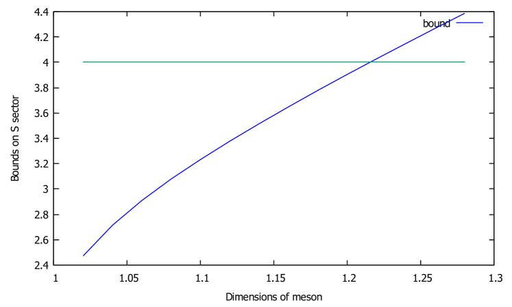
Figure 51: (Color online) Upper bound on the dimension of the first singlet operator appearing in the OPE $\Phi\times\bar{\Phi}$ for $N=8$, as a function of $\Delta_{\Phi}$ Nakayama (2016b).

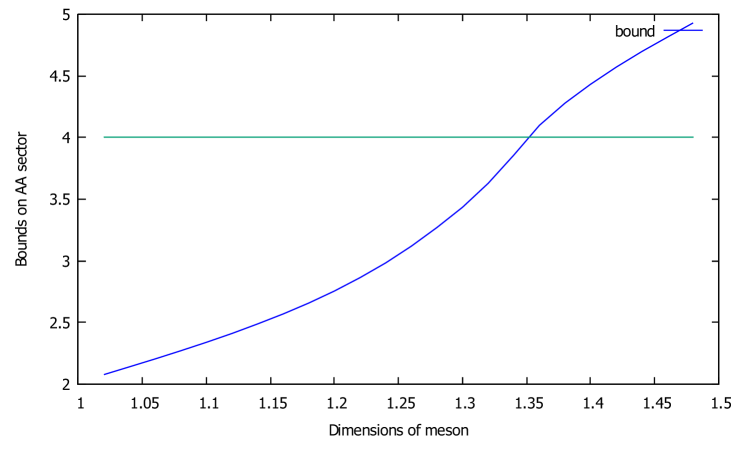
Figure 52: (Color online) Upper bounds on the dimensions of the first TT and AA operators appearing in the OPE $\Phi\times\bar{\Phi}$ for $N=8$, as a function of $\Delta_{\Phi}$ Nakayama (2016b).

Nakayama (2016b) also derived, under the same assumptions, upper bounds on the lowest scalars in $\Phi\times\bar{\Phi}$ which transform as $TT$ or $AA$ under $H$, where $T/A$ stands for the symmetric/antisymmetric traceless tensor representation. See Fig. 52 for the bound at $N=8$. By an idea of Iha et al. (2016), such bounds constrain possible global symmetry enhancements, in parallel with Sec. V.5.3. Namely, imagine that we are trying to reach the CFT describing the Banks-Zaks fixed point in an RG flow from a microscopic description which at short distances preserves only a subgroup $H^{\prime}$ of $H$, as well as parity. For example, this would be true for lattice studies with Wilson or domain wall fermions, which only realize the diagonal subgroup

$$H^{\prime}_{\rm Wilson}=SU(N)_{V}\,,$$ (131)

as in Ishikawa et al. (2014, 2015). A second example is furnished by staggered fermions, another lattice fermion realization commonly used to study the QCD₄ conformal window. Being defined for $N$ a multiple of 4, these preserve microscopically a subgroup

$$H^{\prime}_{\rm staggered}=SU(N/4)\times SU(N/4)\,.$$ (132)

Observing the Banks-Zaks fixed point in a lattice Monte Carlo simulation using a fermion realization with a reduced symmetry implies a symmetry enhancement. For this to be possible, all parity-even scalar operators which are singlets under $H^{\prime}$ (but not necessarily under $H$) must be irrelevant. Since the $TT$ and $AA$ representations of $H$ contain a singlet when reduced under either Eqs. (131) or (132), we obtain a necessary condition that the $TT$ and $AA$ scalars must be irrelevant in both cases. So, from the $TT$ bound in Fig. 52, enhancement from $H^{\prime}_{\rm Wilson}$ or $H^{\prime}_{\rm staggered}$ requires

$$\text{Wilson or staggered}\ \Rightarrow\ \Delta_{\Phi}>1.69\ (N=8)\,.$$ (133)

Compared to Nakayama (2016b), the earlier analysis of symmetry enhancement bounds for lattice QCD by Iha et al. (2016) did not use the full symmetry $H$ but only the vectorial subgroup $SU(N)_{V}$, grouping the operators (129) into the irreducible representations of $SU(N)_{V}\times P$,

$$S=\sum_{j=1}^{N}\bar{\psi}^{\bar{j}}\psi_{j}\,,\quad\quad S^{\bar{k}}_{i}=\bar{\psi}^{\bar{k}}\psi_{i}-\frac{1}{N}\delta^{\bar{k}}_{i}S\,,$$

$$\phi=\sum_{j=1}^{N}\bar{\psi}^{\bar{j}}\gamma_{5}\psi_{j}\,,\quad\quad \phi^{\bar{k}}_{i}=\bar{\psi}^{\bar{k}}\gamma_{5}\psi_{i}-\frac{1}{N}\delta^{\bar{k}}_{i}\phi\,,$$

which transform as singlets or adjoints under $SU(N)_{V}$, and have $P=\pm$. This simplifies the analysis, as the system of crossing relations for representations of $SU(N)_{V}$ is easier than for the full $H$. Of course, by not using the full symmetry one loses information, although this can be partially remedied by imposing by hand the constraint that all operators in Eq. (VI.3) have the same dimension.

In this setup Iha et al. (2016) could extract bounds from the symmetry enhancement for staggered fermions (but not for Wilson fermions). To do this they analyzed the 4pt function of the adjoint pseudoscalar $\phi^{\bar{k}}_{i}$ for $N=8,12,16$. They derived upper bounds on the lowest dimension scalar in the $\phi\times\phi$ OPE transforming in the representation $[N-1,N-1,1,1]$ of $SU(N)_{V}$. They argued that symmetry enhancement requires that this scalar be irrelevant.

To illustrate this more clearly, using results of Lee and Sharpe (1999) they identified explicitly some four-fermion operators which are singlets under (132) and which have nonzero overlap with $[N-1,N-1,1,1]$ when the symmetry is reduced to $SU(N)_{V}$. The resulting necessary condition for staggered fermion enhancement is:

$$\text{Staggered}\ \Rightarrow\ \Delta_{\Phi}>1.67,1.71,1.71\ (N=8,12,16)\,.\ \qquad$$ (135)

That for $N=8$ this bound is somewhat weaker than Eq. (133) is explained partly by not using the full symmetry, and partly by working at a lower derivative order.

It should be mentioned that most studies of the QCD conformal window by lattice Monte Carlo or RG methods point to rather small anomalous dimensions $\gamma_{\Phi}$. Hence the above bootstrap bounds on $\Delta_{\Phi}$ are probably not optimal. Finding better bootstrap constraints on the QCD conformal window is an interesting open problem. Some possibilities to make further progress are to pursue mixed correlator studies, to include global symmetry currents and the stress-tensor in the bootstrap (whose 3pt functions contain known anomaly coefficients), and/or to study baryon operators.

VII Applications to superconformal theories

Conformal symmetry admits a supersymmetric extension into a superalgebra containing the standard anticommuting supercharges $\{\mathcal{Q},\bar{\mathcal{Q}}\}\sim P$ as well as $R$-symmetry generators and the anticommuting analog of SCTs $\{\mathcal{S},\bar{\mathcal{S}}\}\sim K$ (called special superconformal transformations). Superconformal field theories (SCFTs) are extraordinarily rich, and have been studied intensively from many viewpoints. In the last decades the zoo of known theories has grown in size: new constructions have been made, including many Lagrangian models, but remarkably also many theories that appear to admit no such description have been found. Also, a great number of strongly coupled SCFTs are known to exist, in different dimensions and with different number of supercharges, some of which can be understood using field theory or holographic dualities.

SCFTs represent an important playground to test our understanding of CFTs and the effectiveness of bootstrap techniques. The presence of supersymmetry allows one to exactly compute some interesting CFT data, even in a strongly interacting regime, which in turn can be compared with bootstrap predictions.

From the point of view of the conformal bootstrap, supersymmetry has essentially three consequences: 1) relating the OPE coefficients and dimensions of operators belonging to the same supersymmetric multiplet, creating superconformal blocks; 2) acting as a selection rule for the operators entering a given OPE and imposing stronger constraints from unitarity; 3) fixing the dimensions of certain short multiplets. By virtue of these constraints, crossing symmetry is expected to be more effective in SCFTs.

VII.1 Theories with 4d $\mathcal{N}=1$ supersymmetry

Before discussing the numerical bootstrap results, let us spend a few words on the structure of representations of the superconformal algebra. For concreteness we will give this discussion for SCFTs with 4d $\mathcal{N}=1$ supersymmetry. Superconformal primary operators (annihilated by the special superconformal generators $\cal S,\bar{\cal S}$) are labelled by four numbers $(q,\bar{q},\ell,\bar{\ell})$, where $\ell,\bar{\ell}$ are the usual Lorentz quantum numbers and $q,\bar{q}$ are related to the scaling dimension $\Delta$ and $R-$charge of the superconformal primary operator:

$$\Delta=q+\bar{q}\qquad R=\frac{2}{3}(q-\bar{q})\,.$$ (136)

Unitarity bounds on these operators were worked out by Flato and Fronsdal (1984) and Dobrev and Petkova (1985), taking the form

$$q\geqslant\frac{1}{2}\ell+1\,,\,\bar{q}\geqslant\frac{1}{2}\bar{\ell}+1 (\ell\bar{\ell}\neq 0)\,,$$

$$q\geqslant\frac{1}{2}\ell+1 (\bar{q}=\bar{\ell}=0)\,,$$ (137)

$$\bar{q}\geqslant\frac{1}{2}\bar{\ell}+1 (q=\ell=0)\,.$$

The second and third lines in the above expression identify chiral ($\Phi_{\alpha_{1}....\alpha_{\ell}}$) or antichiral ($\bar{\Phi}_{\dot{\alpha}_{1}....\dot{\alpha}_{\bar{\ell}}}$) operators, which are annihilated by the supercharge $\bar{\mathcal{Q}}$ or $\mathcal{Q}$, respectively.

Finally, we would like to mention a few theoretical results for superconformal blocks present in the literature, focusing on those relevant for the 4d $\mathcal{N}=1$ bootstrap. Superconformal blocks for correlation function of scalar superconformal primaries can be expressed in terms of finite linear combinations of ordinary scalar conformal blocks with suitable dimensions and spin; however, computing these coefficients can be a challenging task. The work of Poland and Simmons-Duffin (2011); Vichi (2012) obtained the superconformal blocks for 4pt functions of a scalar chiral supermultiplet $\Phi$. Shortly after, Fortin et al. (2011) computed superconformal blocks for 4pt functions of the multiplet associated to global symmetry conserved currents, whose lowest component is again a scalar field. A similar analysis applicable to 4pt functions of $R$-current multiplets (containing the stress tensor) was also recently carried out in Manenti et al. (2018). The general approach in these works was to classify the possible 3-point functions in superspace using the formalism of Osborn (1999) and then expand in the Grassmann variables $\theta_{i}$ to compute relations between OPE coefficients of conformal primaries. In this approach one must also carefully compute the norm of each conformal primary in the multiplet.

The work of Fitzpatrick et al. (2014a) developed alternate techniques based on either solving the super-Casimir equation or writing the blocks as superconformal integrals using a super-embedding formalism. The latter approach was employed in Khandker et al. (2014) to find the blocks appearing in the more general correlation function $\langle\Phi_{1}\bar{\Phi}_{2}\Psi_{1}\bar{\Psi}_{2}\rangle$, where $\Phi_{i}$ and $\Psi_{i}$ are scalar superconformal primary operators with arbitrary dimension and $R$-charge, with the restriction that the exchanged operator is neutral under $R$-symmetry. This analysis was later extended in Li and Su (2016) to the more general case of four distinct scalar superconformal primary operators with arbitrary scaling dimensions and $R$-charges, with no restriction on the exchanged operators besides those imposed by superconformal symmetry. However, this analysis was missing a particular class of superconformal blocks, associated to exchanged primaries in representations of the Lorentz group with $\ell\neq\bar{\ell}$. In this case the corresponding superconformal primary does not enter the OPE of the external operators, but some of its superconformal descendants do. This issue was fixed in Li et al. (2017b).

VII.1.1 Bounds without global symmetries

Now we will summarize numerical results for correlation functions involving scalar chiral superfields. The first numerical studies, starting with Poland and Simmons-Duffin (2011) and improved in Vichi (2012) and Poland et al. (2012), focused on 4pt functions containing a single scalar chiral supermultiplet $\langle\Phi\bar{\Phi}\Phi\bar{\Phi}\rangle$. Crossing symmetry for this correlation function involves two OPE channels. Because of the chirality conditions, the $\Phi\times\bar{\Phi}$ OPE only receives contributions from traceless symmetric tensor superconformal primaries together with their $\mathcal{Q}\bar{\mathcal{Q}}$ and $\mathcal{Q}^{2}\bar{\mathcal{Q}}^{2}$ superdescendants, giving rise to the superconformal blocks described above. The $\Phi\times\Phi$ OPE on the other hand is more subtle and can receive three different contributions: 1) the chiral superfield $\Phi^{2}$; 2) $\bar{\mathcal{Q}}$ descendants of semi-short multiplets; 3) $\bar{\mathcal{Q}}^{2}$ descendants of generic (long) multiplets. As a result, this channel allows conformal blocks of even spin $\ell=\bar{\ell}$ at either the protected dimensions $\Delta=2\Delta_{\Phi}+\ell$ or at unprotected dimensions satisfying the unitarity bound $\Delta\geqslant|2\Delta_{\Phi}-3|+\ell+3$.

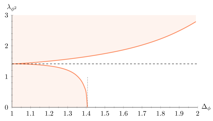
(a) (b)

Figure 53: (Color online) (a) Upper bound on the dimension of the operator $\mathcal{R}$ as a function of $\Delta_{\Phi}$ Poland et al. (2012); Li et al. (2017b). The shaded area is excluded. The dashed line at $\Delta_{\mathcal{R}}=2\Delta_{\Phi}$ corresponds to generalized free theories. (b) Lower and upper bounds on the OPE coefficient of the chiral operator $\Phi^{2}$ entering the $\Phi\times\Phi$ OPE. The vertical dotted line is at $\Delta_{\Phi}=1.407$ and the horizontal dashed line is at the free theory value $\lambda_{\Phi\Phi\Phi^{2}}\equiv\lambda_{\phi}^{2}=\sqrt{2}$ Poland and Stergiou (2015).

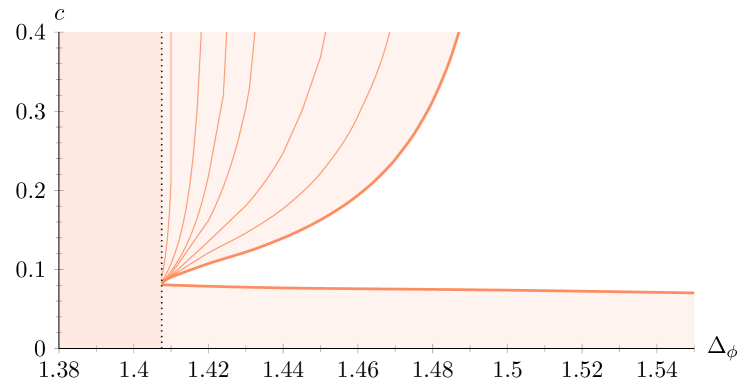
(a) (b)

Figure 54: (Color online) (a) Lower bound on the central charge as a function of $\Delta_{\Phi}$ assuming that $\Delta_{\mathcal{R}}$ is consistent with the unitarity bound (thin line) or it saturates the upper bound in Fig. 53 (thick line). The shaded area is excluded Li et al. (2017b). (b) Lower and upper bounds on the central charge as a function of $\Delta_{\Phi}$, with the assumption that there is no $\Phi^{2}$ operator. The upper bounds correspond to different gaps until the second spin-1 superconformal primary $\Delta_{\ell=1}\geqslant 3.1,3.3,3.5,3.7,3.9,4,4.1$ (from left to right). The shaded area is excluded Poland and Stergiou (2015).

In Fig. 53 we show an upper bound on the dimension of the first real scalar supermultiplet $\mathcal{R}$ entering the OPE $\Phi\times\bar{\Phi}$. A first important consequence of this result is that in any perturbative SCFT, the combination $2\Delta_{\Phi}-\Delta_{\mathcal{R}}$ must be positive (or very suppressed) to satisfy the bound. Secondly, one can observe a minor kink-like feature on the boundary of the allowed region. The same feature appears in the lower bound on the central charge, Fig 54, and it also coincides with the minimal value of $\Delta_{\Phi}$ consistent with the absence of the chiral operator $\Phi^{2}$, as shown in the bottom panel of Fig 53.

In light of this, it is tempting to conjecture the existence of a “minimal SCFT” that realizes the chiral ring relation $\Phi^{2}=0$ and saturates these bounds. This conjecture has been seriously addressed by Poland and Stergiou (2015) and Li et al. (2017b), who studied the properties of this hypothetical theory. Notice that the minimal value of $\Delta_{\Phi}$ consistent with the chiral ring assumption, let us call it $\Delta_{\Phi}^{\text{mSCFT}}$, represents an extremal solution, and it is therefore uniquely determined. In addition, to coincide with the kinks it should agree with the solution obtained from maximizing the dimension of the first neutral unprotected operator and the solution obtained from minimizing the central charge, at the same value of $\Delta_{\Phi}$.

Fig 54 (a) shows that the two extremization procedures generically lead to two different solutions, except at $\Delta_{\Phi}^{\text{mSCFT}}$. This confirms our expectation of a unique solution coinciding with the kinks. Furthermore, by inputting a gap between the stress-tensor multiplet (whose lowest component is the spin-1 $U(1)_{R}$ current) and the next spin-1 supermultiplet, one is able to extract an upper bound on the central charge. While this bound is gap-dependent at generic $\Delta_{\Phi}$, it almost coincides with the lower bound at $\Delta_{\Phi}^{\text{mSCFT}}$, as shown in Fig 54 (b). By extrapolating these results at large $\Lambda$, Poland and Stergiou (2015) obtained the prediction $\Delta_{\Phi}^{\text{mSCFT}}\approx 1.428,\,c\approx 0.111$, perhaps consistent with $\Delta_{\Phi}^{\text{mSCFT}}=10/7,\,c=1/9$.

Recently a few theories have been proposed as mSCFT candidates Xie and Yonekura (2016); Buican and Nishinaka (2016), which implement the chiral ring condition $\Phi^{2}=0$; however, they don’t quite match the bootstrap predictions presented here. In particular the central charge is much larger than $1/9$.

It is also worth noticing that, in any solution saturating the dimension bound of Fig. 53, the chiral operator $\Phi$ is not charged under any global symmetry. If it was, in fact, the solution would contain a spin-$1$ conserved current, which in $\mathcal{N}=1$ SUSY happens to be the superdescendant of a dimension-2 real scalar which would appear in the $\Phi\times\bar{\Phi}$ OPE.

To conclude this section, let us mention that the work of Li et al. (2017b) also performed a bootstrap study of a system of mixed correlators involving a scalar chiral superfield $\Phi$ and a long real scalar superfied $\mathcal{R}$, identified with the first scalar operator appearing in the $\Phi\times\bar{\Phi}$ OPE. Unlike in 3d, this analysis didn’t seem to allow one to easily isolate a closed region. A preliminary inspection of the extremal solution doesn’t reveal any obvious low-lying operators decoupling from the spectrum, but rather it involves a rearrangement of higher dimensional operators Stergiou (2017). It will be interesting to study this rearrangement further and understand how to robustly isolate the conjectured mSCFT in future work.

VII.1.2 Bounds with global symmetries

As mentioned in the previous section, conserved currents of global symmetries $j_{\mu}^{a}$ sit in real supermultiplets $\mathcal{J}^{a}$ whose lowest component is a dimension-2 scalar $J^{a}$. In addition, the multiplet satisfies the conservation condition $D^{2}\mathcal{J}^{a}=\bar{D}^{2}\mathcal{J}^{a}=0$. Bootstrapping correlation functions of the scalars $J^{a}$ allows one access to the space of local SCFTs with a given global symmetry. Hence, due to supersymmetry, one can apply the same machinery encountered so far, with no need to deal with spinning conformal blocks.

Bounds on OPE coefficients of $SU(N)$ currents were explored in Berkooz et al. (2014) and dimension bounds (and coefficient bounds assuming gaps) from single 4pt functions $\langle JJJJ\rangle$ were explored in Li et al. (2017b). The latter work also studied the case of mixed correlators involving $J$ and a chiral field $\Phi$ charged under the global symmetry. Note that this charge necessarily differs from the $R$-symmetry, which instead is part of the conformal algebra: the conserved current associated with the latter is the lowest component of the Ferrara-Zumino multiplet which contains the stress-tensor and supercurrents.

A key result, shown in Fig. 55, shows that any local SCFT with a continuous global symmetry must contain a real scalar multiplet $\mathcal{O}$ with dimension $\Delta_{\mathcal{O}}\leqslant 5.246$. The same figure also shows upper bounds on the OPE coefficient associated to $J$ itself as well as the one associated to the stress tensor multiplet, denoted as $V$. Interestingly, both bounds on $c_{J}$ and $c_{V}$ show plateaus for small values of the gap in the scalar sector. These are perhaps consistent with the existence of SCFT solutions shaping the bounds. On the other hand, the values extracted from Fig. 55 are much smaller then the limits one obtains by inspecting the correlation functions of chiral superfields. For instance, the relation between $c_{V}$ and Fig. 54 is $c_{V}^{2}=1/(90c)$, making the bound on the central charge very weak.

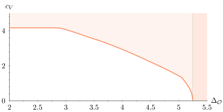
(a) (b)

Figure 55: (Color online) Upper bounds on the OPE coefficients $c_{\mathcal{O}}\equiv 2^{-\ell/2}\lambda_{JJ\mathcal{O}}$ appearing in the $J\times J$ OPE arising from (a) $J$ itself or (b) the stress-tensor supermultiplet $V$, as a function of the dimension of the first unprotected scalar $\mathcal{O}$ in the $J\times J$ OPE. The region to the right of the dotted vertical line at $\Delta_{\mathcal{O}}=5.246$ is not allowed Li et al. (2017b).

An alternative method to study SCFTs with global symmetries is to consider external scalar operators in nontrivial representations of the symmetry. An important target is to make contact with supersymmetric QCD theories, e.g. supersymmetric gauge theories with gauge group $SU(N_{c})$ and $N_{f}$ flavors of quarks $Q_{i},\overline{Q}^{\bar{j}}$, with $N_{f}$ in the conformal window $3N_{c}/2\leqslant N_{f}\leqslant 3N_{c}$ Seiberg (1995). The simplest gauge-invariant operators are the mesons $M_{i}^{\bar{j}}=Q_{i}\overline{Q}^{\bar{j}}$, which transform as bi-fundamentals of $SU(N_{f})_{L}\times SU(N_{f})_{R}$ and have dimension $\Delta_{M}=3(1-N_{c}/N_{f})$. Due to supersymmetry, both the central charge and current central charge can be exactly computed due to their relation to anomaly coefficients.

A partial bootstrap analysis applicable to meson 4pt functions was performed in Poland et al. (2012), which considered chiral scalar multiplets transforming in the fundamental representation of $SU(N)$ and obtained bounds on the OPE coefficients associated to conserved currents transforming in both the singlet and the adjoint representations of $SU(N)$. As can be seen in Fig. 56, these bounds are still somewhat far from the exact results of supersymmetric QCD (SQCD) theories, most likely because this study didn’t utilize the full symmetry. It will be very interesting in future work to extend these analyses of chiral 4pt functions to use the whole SQCD global symmetry, together with mixed correlators containing the $SU(N_{f})_{L/R}$ current multiplets and/or the stress-tensor multiplet.

Figure 56: (Color online) Lower bounds on the effective 2pt function coefficient $\kappa_{\text{eff}}=1/\lambda_{\Phi\Phi J}^{2}$ of $SU(N)$ singlet currents appearing in $\Phi\times\bar{\Phi}$, where $\Phi$ is a chiral scalar of dimension $d$ in the fundamental of $SU(N)$, for $N=2,\ldots,14$. The bounds are normalized to the value $\kappa_{\text{chiral}}$ corresponding to a free chiral superfield. Each dot connected to a bound corresponds to the exact value in an SQCD theory with the same symmetry Poland et al. (2012).

VII.2 Theories with 3d $\mathcal{N}=2$ supersymmetry

Another interesting set of targets for the conformal bootstrap are the zoo of 3d CFTs with $\mathcal{N}=1$ or $\mathcal{N}=2$ supersymmetry. We made initial contact with the former in Sec. V.4.3, where there were no constraints from supersymmetry used other than relations between scaling dimensions (see however footnote 120). The superconformal representation theory of the latter has a similar structure to that of 4d $\mathcal{N}=1$ SCFTs; for details see Minwalla (1998) and Bobev et al. (2015a). Perhaps the simplest such theory is the $\mathcal{N}=2$ supersymmetric Wess-Zumino model described in Sec. V.4.1. This CFT can be thought of as the IR fixed point of a theory of a single chiral superfield $\Phi=\phi+\psi\theta+F\theta^{2}$ and superpotential $W=\lambda\Phi^{3}$. The fixed point has a $U(1)_{R}$ symmetry under which $\Phi$ has charge 2/3, implying exact dimensions for the complex scalar $\phi$ and the Dirac fermion $\psi$: $\Delta_{\phi}=q_{\phi}=2/3$, $\Delta_{\psi}=\Delta_{\phi}+1/2=7/6$.

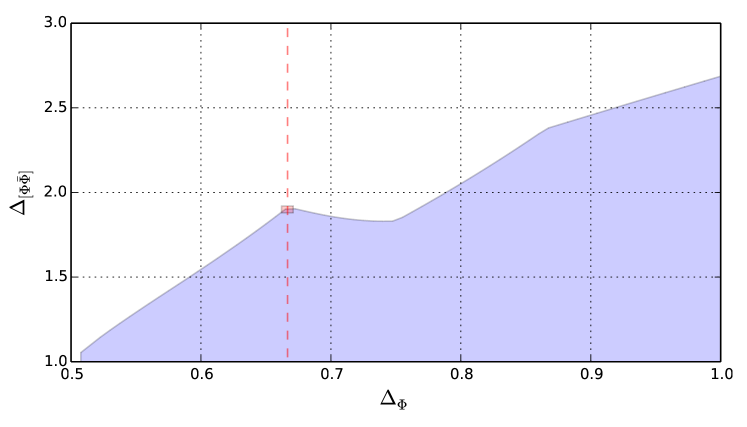
Figure 57: (Color online) Bound on the dimension of the first unprotected scalar $\Phi\bar{\Phi}$ in the $\Phi\times\bar{\Phi}$ OPE in 3d SCFTs with $\mathcal{N}=2$ supersymmetry Bobev et al. (2015b).

Applying the numerical bootstrap to the 4pt function $\langle\Phi\bar{\Phi}\Phi\bar{\Phi}\rangle$ and incorporating the unitarity bounds and superconformal blocks of $\mathcal{N}=2$ superconformal symmetry, Bobev et al. (2015b, a) and Li and Su (2017a) studied general bounds on the dimension of the leading unprotected scalar operator $\Phi\bar{\Phi}$, with the basic result shown in Fig. 57. Curiously, the resulting bound has three distinct features, the first of which occurs at a scaling dimension $\Delta_{\Phi}\simeq 2/3$. This gives a sharp upper bound $\Delta_{\Phi\bar{\Phi}}<1.91$ for the $\mathcal{N}=2$ supersymmetric Wess-Zumino model and a plausible conjecture that the model saturates the optimal version of this bound. Further analysis of the extremal spectrum of this kink can be found in Bobev et al. (2015b, a), while Li and Su (2017a) found that an isolated island around $\{\Delta_{\Phi},\Delta_{\Phi\bar{\Phi}}\}=\{0.6678(13),1.903(10)\}$ could be obtained by assuming a modest gap in the spectrum of spin-1 superconformal primaries $\Delta_{J^{\prime}}\geqslant 3.5$.

The middle kink occurs near $\Delta_{\Phi}=3/4$, and coincides with a kinematic threshold beyond which superconformal descendants of anti-chiral operators $Q^{2}\bar{\Psi}$ can no longer appear in the $\Phi\times\Phi$ OPE. It is not yet clear if any CFT sits at this kink. The right-most kink, occurring near $\Delta_{\Phi}\sim.86$, also still lacks a clear interpretation, but seems to interpolate to the kink in the 4d $\mathcal{N}=1$ bounds discussed above. Notably, the extremal spectrum of this kink seems to satisfy the chiral ring relation $\Phi^{2}=0$ Bobev et al. (2015a) and an island around the point can also be isolated using a set of gap assumptions Li and Su (2017a), making it a plausible candidate for a new CFT. Finally let us mention that this analysis was also extended to 3d $\mathcal{N}=2$ supersymmetric CFTs with $O(N)$ global symmetry by Chester et al. (2016a, b), who found similar features at each value of $N$. A related 3d $\mathcal{N}=2$ theory with multiple interacting chiral superfields and a conformal manifold was also recently studied using bootstrap methods in Baggio et al. (2018).

VIII Applications to nonunitary models

The great majority of numerical conformal bootstrap applications considered to date have concerned unitary CFTs. This limitation was mainly due to the fact that the main two rigorous numerical bootstrap methods, linear programming and semidefinite programming (Sec. IV) require positivity of the squares of OPE coefficients or positive-definiteness of the matrices made of their pairwise products, which only hold in unitary theories. Nevertheless there have been some promising attempts to apply conformal bootstrap methods to nonunitary theories, which we wish to briefly describe here.

One naturally occurring class of nonunitary CFTs are theories analytically continued from integer to noninteger space dimensions $d$, the prime example being the Wilson-Fisher family of fixed points in $2\leqslant d<4$. It was only understood very recently that these CFTs are nonunitary for noninteger $d$.

Fortunately, the violation of unitarity in these theories seems to be rather mild, as the negative-norm operators have rather high dimension Hogervorst et al. (2016). So it is believed that the standard linear and semidefinite programming methods, while non-rigorous in this context, should still give reasonable results. This explains the success of El-Showk et al. (2014a) who found good agreement between the numerical bootstrap and the $\epsilon$-expansion in the whole range $2\leqslant d<4$ using the 4pt function $\langle\sigma\sigma\sigma\sigma\rangle$ and analytically continuing conformal blocks to noninteger $d$. Similarly, Behan (2017a) generalized to noninteger $d$ the multiple-correlator analysis leading to the 3d Ising model island in Fig. 13. A related successful study by Bobev et al. (2015a) analyzed the analytic continuation to $2\leqslant d\leqslant 4$ of theories with 4 supercharges, which for $d=3$ reduces to the ${\cal N}=2$ Wess-Zumino model from Sec. VII.2.

Leaving aside the physical interpretation, the $\mathbb{Z}_{2}$-invariant Wilson-Fisher fixed points can actually be analytically continued even below $d=2$ and perhaps all the way to $d=1^{+}$ Holovatch (1993). Interestingly, the analytic continuation seems to no longer be reproduced by the linear programming bootstrap in $d<2$, likely because violations of unitarity are stronger in this case than for $d\geqslant 2$ Golden and Paulos (2015). This serves as a warning to keep in mind when applying the linear and semidefinite methods to nonunitary theories.

As described in Sec. IV.5, the truncation method should in principle be more suitable for analyzing nonunitary theories. Gliozzi (2013) and Gliozzi and Rago (2014) successfully applied the truncation method to the Lee-Yang CFT, which is a nonunitary CFT describing the IR fixed point of the $\phi^{3}$ scalar theory in $2\leqslant d<6$ dimensions Fisher (1978). Truncating the $\phi\times\phi$ OPE to the identity operator, $\phi$ itself, the stress tensor, and two more operators, estimates of $\Delta_{\phi}$ were obtained in good agreement with RG and lattice predictions, and with the exact solution available for $d=2$.

Finally we mention that bootstrap methods can also be straightforwardly applied to nonunitary CFTs if a reasonable conjecture for the spectrum is available, as happens in the case of 2d percolation Picco et al. (2016). In this special situation, one simply solves crossing relations for the squares of OPE coefficients, with no restriction on sign.

IX Other applications

We would like to finish our review by briefly describing some of the many related topics that we have not been able to cover. Many of these topics have also seen significant recent progress and would merit their own reviews. We hope that we can at a minimum give the reader some useful entry points into the literature.

A traditional approach to learning about CFTs has been to use perturbation theory, often in the context of $\epsilon$-expansions or $1/N$-expansions. There is an older literature about using bootstrap-like techniques to reproduce $1/N$ expansions, see e.g. Lang and Ruhl (1992); Petkou (1996), involving setting up self-consistency equations using a sum over dressed Feynman diagrams sometimes called a “skeleton expansion.” More recently, there have been a number of recent works which use more modern analytical bootstrap techniques to study perturbative expansions, e.g. studying bootstrap equations in a $1/N$ expansion, using conformal invariance and the appearance of null states to reproduce $\epsilon$-expansions, and using a formulation of the bootstrap in Mellin space to reproduce $\epsilon$ and large-$N$ expansions by reviving an old idea by Polyakov (1974) to make crossing symmetry manifest and impose unitarity.

A related analytical approach has been to study bootstrap equations in various Lorentzian limits. One such limit is the lightcone limit developed in Fitzpatrick et al. (2013); Komargodski and Zhiboedov (2013), which has allowed for a systematic study of CFT data in a large spin expansion or with slightly-broken higher spin symmetry in the works Alday and Zhiboedov (2016) and Alday (2017b). Another limit where recent progress has been made is the Regge limit. Both of these limits can be connected to constraints from Lorentzian causality, where nontrivial bounds and sum rules can be derived, yielding new arguments for the conformal collider bounds of Hofman and Maldacena (2008), Buchel et al. (2010), and Chowdhury et al. (2013), as well as the more stringent constraints of Camanho et al. (2016) in holographic theories. Finally we should mention the recent development of a powerful Lorentzian inversion formula as well as related work on higher-dimensional crossing kernels, which are another promising route for further analytical progress.

The conformal bootstrap in two dimensions has a long history, for example the seminal applications to rational CFTs in Belavin et al. (1984). The modern numerical bootstrap has been re-applied to 2d CFTs in a number of works. A related direction is the modular bootstrap, which sets up consistency conditions arising from modular invariance. A number of recent studies have also looked at these constraints using modern numerical bootstrap techniques. A proper summary of these results and related analytical progress in the context of both the history of the 2d bootstrap and holography would merit its own review; see e.g. Yin (2017).

One can also study the conformal bootstrap in more than four dimensions or with extended supersymmetry. One application of the numerical bootstrap has e.g. been to the 6d $(2,0)$ SCFT Beem et al. (2016b), interesting in part because of its non-Lagrangian nature and ability to teach us about new dualities. Another application in $d>4$ has been to probe the existence of $O(N)$ vector models in 5d. Progress has also been made placing constraints on a variety of other 5d and 6d SCFTs, 4d $\mathcal{N}=2$ and $\mathcal{N}=3$ SCFTs, 4d $\mathcal{N}=4$ supersymmetric Yang-Mills theory, and 3d $\mathcal{N}=8$ SCFTs Chester et al. (2014) including ones inspired by M-theory Agmon et al. (2017b). Related analytical progress at solving sub-sectors of SCFTs with extended supersymmetry was also made in Beem et al. (2015a, c); Chester et al. (2015a) and used in a number of follow-up studies.

Work on the superconformal bootstrap (particularly with extended supersymmetry) is not possible without analytical computations of superconformal blocks, which have been developed in a number of works using both superembedding space methods and by solving the superconformal Casimir equation.

Another intriguing line of research is the development of a direct relation between conformal blocks and the wave-functions of integrable Hamiltonians. Finally, while we cannot review here all of the interesting developments in the AdS/CFT correspondence, it is worth mentioning that there has been an abundance of activity in connecting both global blocks and semi-classical Virasoro blocks to geodesics in AdS and bulk semi-classical physics.

All of the conformal bootstrap constraints and numerical bounds we have considered in this review have applied to either Euclidean CFT or relativistic Lorentzian CFT. It is also of great interest to learn about nonrelativistic conformal field theories due to their many experimental realizations, e.g. to ultracold atomic gases near the unitary limit. While nonrelativistic conformal symmetries are inherently less constraining, some important theoretical groundwork on correlation functions and the OPE has been laid for systems governed by the nonrelativistic Schrödinger algebra, which is a necessary precursor to any bootstrap analysis.

Another interesting situation that we have not discussed are systems governed by logarithmic CFTs, a class of nonunitary CFTs describing e.g. models of percolation, self-avoiding random walks, and systems with quenched disorder. While such theories have been considered for a long time in two dimensions (see Creutzig and Ridout (2013) for a review), logarithmic CFTs in higher dimensions have received less attention. A general theoretical analysis of correlation functions in such theories was recently developed in Hogervorst et al. (2017), building on earlier work Ghezelbash and Karimipour (1997). Attempts to apply direct numerical bootstrap to such theories have been mentioned in Sec. VIII. Let us also mention the study Komargodski and Simmons-Duffin (2017) of the Ising model with quenched disorder which made extensive use of bootstrap data to develop an approach based on conformal perturbation theory.

X Outlook

The conformal bootstrap is still in its infancy and there remains much low-hanging fruit to pick along with many important open questions. For instance, can we use the bootstrap to fully classify the space of critical CFTs with a given symmetry, placing universality on a rigorous footing? Can the bootstrap solve the conformal windows of QED₃ and QCD₄? Can it be used as a discovery tool to find new, perhaps non-Lagrangian, CFTs? Is there an analytical understanding of the kinks in numerical bounds or why certain CFTs such as the 3d Ising model live in them? Which CFTs can be found using extremal spectrum or truncation methods? And is there a fruitful way to incorporate developments in the analytical bootstrap with rigorous numerical methods?

For newcomers to the numerical bootstrap who want to quickly get started, after learning CFT basics we recommend becoming familiar with the available software tools, particularly SDPB which is under active development, along with one of the efficient methods to compute conformal blocks in the dimension of interest as described in Sec. III.6. Then one can start reproducing numerical bounds and thinking about how they can be generalized to say something new about situations of physical interest. For this purpose it is also helpful to get used to restating the physical properties of critical systems using symmetries and the spectrum of scaling dimensions, so questions can be sharply rephrased in the language of the bootstrap. Good luck!

Appendix A Embedding formalism

As we saw in Sec. III.1, the conformal group is isomorphic to $SO(d+1,1)$. This suggests that we can avoid complications due to the SCTs acting nonlinearly on $\mathbb{R}^{d}$ by embedding this space into $\mathbb{R}^{d+1,1}$ where the whole conformal group will act linearly. This main idea of the embedding formalism (also called the projective null cone formalism) goes back to Dirac (1936). Here we will only review the main logic and a few fundamental results, see Costa et al. (2011b) for details and Rychkov (2016b) for a pedagogical introduction.

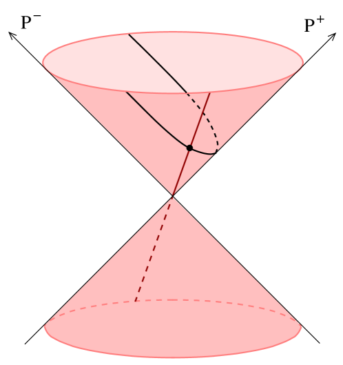
Figure 58: (Color online) The lightcone in the embedding space; light rays are in one-to-one correspondence with points of $\mathbb{R}^{d}$. The Poincaré section of the cone is also shown. Figure from Costa et al. (2011b).

We denote points in the “embedding space” $\mathbb{R}^{d+1,1}$ by $P^{A}$, and use the lightcone coordinates:

$$P^{A}=(P^{+},P^{-},P^{\mu}),\quad P^{\pm}=P^{d+2}\pm P^{d+1},$$

$$P^{2}=P^{\mu}P_{\mu}-P^{+}P^{-}\,.$$ (138)

In this space we consider the “null cone” defined by the equation $P^{2}=0$. The physical space $\mathbb{R}^{d}$ is identified with the “Poincaré section” of the cone given by the equation:

$$P^{A}=(1,x^{2},x^{\mu})\,,\quad x^{\mu}\in\mathbb{R}^{d}\,.$$ (139)

This identification is natural because, as is easy to check, the flat Minkowski metric in $\mathbb{R}^{d+1,1}$ induces a flat $d$-dimensional metric on the Poincaré section (see Fig. 58).

$SO(d+1,1)$ acts naturally on the null rays forming the null cone, and this defines an action on the Poincaré section by picking the intersection point. One can verify that this action realizes a conformal transformation of $\mathbb{R}^{d}$.

Similarly, operators in $d$ dimensions can be lifted to the embedding space. Focusing on traceless symmetric tensors, $\mathcal{O}_{\Delta,\ell}^{\mu_{1}\ldots\mu_{\ell}}(x)$ is promoted to a traceless symmetric tensor $\widehat{\mathcal{O}}_{\Delta,\ell}^{A_{1}\ldots A_{\ell}}(P)$, transforming linearly under $SO(d+1,1)$. The latter operator is required to be homogeneous of degree $-\Delta$:

$$\widehat{\mathcal{O}}_{\Delta,\ell}^{A_{1}\ldots A_{\ell}}(\lambda P)=\lambda^{-\Delta}\widehat{\mathcal{O}}_{\Delta,\ell}^{A_{1}\ldots A_{\ell}}(P)\,.$$ (140)

The relation between the two operators is obtained by the projection

$$\mathcal{O}_{\Delta,\ell}^{\mu_{1}\ldots\mu_{\ell}}(x)=\frac{\partial P_{A_{1}}}{\partial x_{\mu_{1}}}\cdots\frac{\partial P_{A_{\ell}}}{\partial x_{\mu_{\ell}}}\widehat{\mathcal{O}}_{\Delta,\ell}^{A_{1}\ldots A_{\ell}}(P)\,,$$ (141)

where $P$ is restricted to the Poincaré section so that $\frac{\partial P_{A}}{\partial x_{\mu}}=(0,2x_{\mu},\delta_{\mu}^{\alpha})$ . This is consistent with the symmetric traceless condition. Notice as well that two embedding space tensors which differ by anything proportional to $P^{A}$ project to the same physical space tensor, because $P^{A}\partial P_{A}/\partial x_{\mu}=0$. This is sometimes referred to as “gauge freedom”, and it ensures that both representations have the same number of physical components.

The main advantage of this formalism is that the embedding space operators transform linearly under the conformal group. Thus, the problem of classifying correlation functions in embedding space is reduced to finding covariant tensors of $SO(d+1,1)$. In the index free notation, this is equivalent to constructing invariant polynomials depending on the position vectors $P_{A}$ and the polarization vectors $Z_{A}$, with the correct homogeneity properties (140). For traceless tensors it is enough to work with null polarization vectors $Z^{2}=0$. Due to the above mentioned “gauge freedom”, it is also enough to restrict to transverse polarizations: $Z\cdot P=0$. In these conventions, all correlation functions can be built of the basic building blocks Costa et al. (2011b)

$$H_{ij} \equiv\frac{(Z_{i}\cdot Z_{j})(P_{i}\cdot P_{j})-(Z_{i}\cdot P_{j})(Z_{j}\cdot P_{i})}{(P_{i}\cdot P_{j})}\,,$$

$$V_{i,jk} \equiv\frac{(Z_{i}\cdot P_{j})(P_{i}\cdot P_{k})-(Z_{i}\cdot P_{k})(P_{i}\cdot P_{j})}{\sqrt{-2(P_{i}\cdot P_{j})(P_{i}\cdot P_{k})(P_{j}\cdot P_{k})}}\,.$$ (142)

In particular we have $(P_{ij}\equiv-2P_{i}\cdot P_{j})$

$$\langle\widehat{O}_{\Delta,\ell}(P_{1},Z_{1})\widehat{O}_{\Delta,\ell} (P_{2},Z_{2})\rangle=\frac{(H_{12})^{\ell}}{P_{12}^{\Delta}}\,,$$ (143)

$$\langle\widehat{O}_{\Delta_{1}}(P_{1})\widehat{O}_{\Delta_{2}}(P_{2})\widehat{O}_{\Delta_{3}} (P_{3},Z_{3})\rangle=$$ (144)

$$\lambda_{123}\frac{(V_{3,12})^{\ell}}{P_{12}^{h_{123}+\ell}P_{13}^{h_{132}-\ell}\,P_{23}^{h_{231}-\ell}}\,.$$

Projecting to $\mathbb{R}^{d}$ gives Eqs. (22) and (23).

Operators transforming in other $SO(d)$ representations can also be lifted to the embedding space, see e.g. Costa and Hansen (2015) for mixed-symmetry tensors. One can also construct other types of embedding spaces which may be more convenient for dealing with fermions, for supersymmetric CFTs, or in specific $d$.

References

- Afkhami-Jeddi et al. (2017a) Afkhami-Jeddi, Nima, Thomas Hartman, Sandipan Kundu, and Amirhossein Tajdini (2017a), “Einstein gravity 3-point functions from conformal field theory,” JHEP 12, 049, arXiv:1610.09378 [hep-th] .
- Afkhami-Jeddi et al. (2017b) Afkhami-Jeddi, Nima, Thomas Hartman, Sandipan Kundu, and Amirhossein Tajdini (2017b), “Shockwaves from the Operator Product Expansion,” arXiv:1709.03597 [hep-th] .
- Agmon et al. (2017a) Agmon, Nathan B, Shai M. Chester, and Silviu S. Pufu (2017a), “A New Duality Between Superconformal Field Theories in Three Dimensions,” arXiv:1708.07861 [hep-th] .
- Agmon et al. (2017b) Agmon, Nathan B, Shai M. Chester, and Silviu S. Pufu (2017b), “Solving M-theory with the Conformal Bootstrap,” arXiv:1711.07343 [hep-th] .
- Aharony (2016) Aharony, Ofer (2016), “Baryons, monopoles and dualities in Chern-Simons-matter theories,” JHEP 02, 093, arXiv:1512.00161 [hep-th] .
- Aharony et al. (2017a) Aharony, Ofer, Luis F. Alday, Agnese Bissi, and Eric Perlmutter (2017a), “Loops in AdS from Conformal Field Theory,” JHEP 07, 036, arXiv:1612.03891 [hep-th] .
- Aharony et al. (2017b) Aharony, Ofer, Francesco Benini, Po-Shen Hsin, and Nathan Seiberg (2017b), “Chern-Simons-matter dualities with and gauge groups,” JHEP 02, 072, arXiv:1611.07874 [cond-mat.str-el] .
- Alba and Diab (2016) Alba, Vasyl, and Kenan Diab (2016), “Constraining conformal field theories with a higher spin symmetry in ,” JHEP 03, 044, arXiv:1510.02535 [hep-th] .
- Alday (2017a) Alday, Luis F (2017a), “Large Spin Perturbation Theory for Conformal Field Theories,” Phys. Rev. Lett. 119 (11), 111601, arXiv:1611.01500 [hep-th] .
- Alday (2017b) Alday, Luis F (2017b), “Solving CFTs with Weakly Broken Higher Spin Symmetry,” JHEP 10, 161, arXiv:1612.00696 [hep-th] .
- Alday and Bissi (2014) Alday, Luis F, and Agnese Bissi (2014), “The superconformal bootstrap for structure constants,” JHEP 09, 144, arXiv:1310.3757 [hep-th] .
- Alday and Bissi (2015) Alday, Luis F, and Agnese Bissi (2015), “Generalized bootstrap equations for SCFT,” JHEP 02, 101, arXiv:1404.5864 [hep-th] .
- Alday and Bissi (2017) Alday, Luis F, and Agnese Bissi (2017), “Crossing symmetry and Higher spin towers,” JHEP 12, 118, arXiv:1603.05150 [hep-th] .
- Alday et al. (2015a) Alday, Luis F, Agnese Bissi, and Tomasz Lukowski (2015a), “Large spin systematics in CFT,” JHEP 11, 101, arXiv:1502.07707 [hep-th] .
- Alday et al. (2015b) Alday, Luis F, Agnese Bissi, and Tomasz Lukowski (2015b), “Lessons from crossing symmetry at large N,” JHEP 06, 074, arXiv:1410.4717 [hep-th] .
- Alday et al. (2017) Alday, Luis F, Agnese Bissi, and Eric Perlmutter (2017), “Holographic Reconstruction of AdS Exchanges from Crossing Symmetry,” JHEP 08, 147, arXiv:1705.02318 [hep-th] .
- Alday and Zhiboedov (2016) Alday, Luis F, and Alexander Zhiboedov (2016), “Conformal Bootstrap With Slightly Broken Higher Spin Symmetry,” JHEP 06, 091, arXiv:1506.04659 [hep-th] .
- Alday and Zhiboedov (2017) Alday, Luis F, and Alexander Zhiboedov (2017), “An Algebraic Approach to the Analytic Bootstrap,” JHEP 04, 157, arXiv:1510.08091 [hep-th] .
- Alkalaev (2016) Alkalaev, K B (2016), “Many-point classical conformal blocks and geodesic networks on the hyperbolic plane,” JHEP 12, 070, arXiv:1610.06717 [hep-th] .
- Alkalaev and Belavin (2015) Alkalaev, K B, and V. A. Belavin (2015), “Classical conformal blocks via AdS/CFT correspondence,” JHEP 08, 049, arXiv:1504.05943 [hep-th] .
- Alkalaev and Belavin (2016a) Alkalaev, K B, and V. A. Belavin (2016a), “From global to heavy-light: 5-point conformal blocks,” JHEP 03, 184, arXiv:1512.07627 [hep-th] .
- Alkalaev and Belavin (2016b) Alkalaev, K B, and V. A. Belavin (2016b), “Holographic interpretation of 1-point toroidal block in the semiclassical limit,” JHEP 06, 183, arXiv:1603.08440 [hep-th] .
- Alkalaev and Belavin (2017) Alkalaev, K B, and V. A. Belavin (2017), “Holographic duals of large-c torus conformal blocks,” JHEP 10, 140, arXiv:1707.09311 [hep-th] .
- Alkalaev et al. (2017) Alkalaev, K B, R. V. Geiko, and V. A. Rappoport (2017), “Various semiclassical limits of torus conformal blocks,” JHEP 04, 070, arXiv:1612.05891 [hep-th] .
- Alkalaev and Belavin (2016c) Alkalaev, Konstantin B, and V. A. Belavin (2016c), “Monodromic vs geodesic computation of Virasoro classical conformal blocks,” Nucl. Phys. B904, 367–385, arXiv:1510.06685 [hep-th] .
- Andrews (1869) Andrews, Thomas (1869), “The Bakerian Lecture: On the Continuity of the Gaseous and Liquid States of Matter,” Phil. Trans. R. Soc. Lond. 159, 575–590.
- Anous et al. (2018) Anous, Tarek, Raghu Mahajan, and Edgar Shaghoulian (2018), “Parity and the modular bootstrap,” arXiv:1803.04938 [hep-th] .
- Apolo (2017) Apolo, Luis (2017), “Bounds on CFTs with algebras and AdS3 higher spin theories,” Phys. Rev. D96 (8), 086003, arXiv:1705.10402 [hep-th] .
- Appelquist et al. (2017) Appelquist, Thomas, James Ingoldby, and Maurizio Piai (2017), “Dilaton EFT Framework For Lattice Data,” JHEP 07, 035, arXiv:1702.04410 [hep-ph] .
- Appelquist et al. (2018) Appelquist, Thomas, James Ingoldby, and Maurizio Piai (2018), “Analysis of a Dilaton EFT for Lattice Data,” JHEP 03, 039, arXiv:1711.00067 [hep-ph] .
- Appelquist and Nash (1990) Appelquist, Thomas, and Daniel Nash (1990), “Critical Behavior in (2+1)-dimensional QCD,” Phys. Rev. Lett. 64, 721.
- Appelquist et al. (1988) Appelquist, Thomas, Daniel Nash, and L. C. R. Wijewardhana (1988), “Critical Behavior in (2+1)-Dimensional QED,” Phys. Rev. Lett. 60, 2575.
- Atanasov et al. (2018) Atanasov, Alexander, Aaron Hillman, and David Poland (2018), “Bootstrapping the Minimal 3D SCFT,” arXiv:1807.05702 [hep-th] .
- Bae et al. (2017) Bae, Jin-Beom, Sungjay Lee, and Jaewon Song (2017), “Modular Constraints on Conformal Field Theories with Currents,” JHEP 12, 045, arXiv:1708.08815 [hep-th] .
- Bae and Rey (2014) Bae, Jin-Beom, and Soo-Jong Rey (2014), “Conformal Bootstrap Approach to O(N) Fixed Points in Five Dimensions,” arXiv:1412.6549 [hep-th] .
- Baggio et al. (2018) Baggio, Marco, Nikolay Bobev, Shai M. Chester, Edoardo Lauria, and Silviu S. Pufu (2018), “Decoding a Three-Dimensional Conformal Manifold,” JHEP 02, 062, arXiv:1712.02698 [hep-th] .
- Bak et al. (1987) Bak, Per, Chao Tang, and Kurt Wiesenfeld (1987), “Self-organized criticality: An explanation of the 1/f noise,” Phys. Rev. Lett. 59, 381–384.
- Banerjee et al. (2016) Banerjee, Pinaki, Shouvik Datta, and Ritam Sinha (2016), “Higher-point conformal blocks and entanglement entropy in heavy states,” JHEP 05, 127, arXiv:1601.06794 [hep-th] .
- Banks and Zaks (1982) Banks, Tom, and A. Zaks (1982), “On the Phase Structure of Vector-Like Gauge Theories with Massless Fermions,” Nucl. Phys. B196, 189–204.
- Bashkirov (2013) Bashkirov, Denis (2013), “Bootstrapping the SCFT in three dimensions,” arXiv:1310.8255 [hep-th] .
- Basile et al. (2005) Basile, Francesco, Andrea Pelissetto, and Ettore Vicari (2005), “The Finite-temperature chiral transition in QCD with adjoint fermions,” JHEP 02, 044, arXiv:hep-th/0412026 [hep-th] .
- Basile et al. (2006) Basile, Francesco, Andrea Pelissetto, and Ettore Vicari (2006), “Finite-temperature chiral transition in QCD with quarks in the fundamental and adjoint representation,” Proceedings, 23rd International Symposium on Lattice field theory (Lattice 2005): Dublin, Ireland, Jul 25-30, 2005, PoS LAT2005, 199, arXiv:hep-lat/0509018 [hep-lat] .
- Basu and Krishnan (2015) Basu, Pallab, and Chethan Krishnan (2015), “-expansions near three dimensions from conformal field theory,” JHEP 11, 040, arXiv:1506.06616 [hep-th] .
- Bateman (1910) Bateman, H (1910), “The transformation of the electrodynamical equations,” Proc. London Math. Society s2-8 (1), 223–264.
- Baxter (1989) Baxter, R J (1989), Exactly solved models in statistical mechanics (Academic Press).
- Beem et al. (2015a) Beem, Christopher, Madalena Lemos, Pedro Liendo, Wolfger Peelaers, Leonardo Rastelli, and Balt C. van Rees (2015a), “Infinite Chiral Symmetry in Four Dimensions,” Commun. Math. Phys. 336 (3), 1359–1433, arXiv:1312.5344 [hep-th] .
- Beem et al. (2016a) Beem, Christopher, Madalena Lemos, Pedro Liendo, Leonardo Rastelli, and Balt C. van Rees (2016a), “The superconformal bootstrap,” JHEP 03, 183, arXiv:1412.7541 [hep-th] .
- Beem et al. (2016b) Beem, Christopher, Madalena Lemos, Leonardo Rastelli, and Balt C. van Rees (2016b), “The (2, 0) superconformal bootstrap,” Phys. Rev. D93 (2), 025016, arXiv:1507.05637 [hep-th] .
- Beem et al. (2017a) Beem, Christopher, Wolfger Peelaers, and Leonardo Rastelli (2017a), “Deformation quantization and superconformal symmetry in three dimensions,” Commun. Math. Phys. 354 (1), 345–392, arXiv:1601.05378 [hep-th] .
- Beem et al. (2015b) Beem, Christopher, Wolfger Peelaers, Leonardo Rastelli, and Balt C. van Rees (2015b), “Chiral algebras of class S,” JHEP 05, 020, arXiv:1408.6522 [hep-th] .
- Beem and Rastelli (2017) Beem, Christopher, and Leonardo Rastelli (2017), “Vertex operator algebras, Higgs branches, and modular differential equations,” arXiv:1707.07679 [hep-th] .
- Beem et al. (2013) Beem, Christopher, Leonardo Rastelli, and Balt C. van Rees (2013), “The Superconformal Bootstrap,” Phys.Rev.Lett. 111, 071601, arXiv:1304.1803 [hep-th] .
- Beem et al. (2015c) Beem, Christopher, Leonardo Rastelli, and Balt C. van Rees (2015c), “ symmetry in six dimensions,” JHEP 05, 017, arXiv:1404.1079 [hep-th] .
- Beem et al. (2017b) Beem, Christopher, Leonardo Rastelli, and Balt C. van Rees (2017b), “More superconformal bootstrap,” Phys. Rev. D96 (4), 046014, arXiv:1612.02363 [hep-th] .
- Behan (2017a) Behan, Connor (2017a), “PyCFTBoot: A flexible interface for the conformal bootstrap,” Commun. Comput. Phys. 22 (1), 1–38, arXiv:1602.02810 [hep-th] .
- Behan (2017b) Behan, Connor (2017b), “The unitary subsector of generalized minimal models,” arXiv:1712.06622 [hep-th] .
- Behan et al. (2017a) Behan, Connor, Leonardo Rastelli, Slava Rychkov, and Bernardo Zan (2017a), “A scaling theory for the long-range to short-range crossover and an infrared duality,” J. Phys. A50 (35), 354002, arXiv:1703.05325 [hep-th] .
- Behan et al. (2017b) Behan, Connor, Leonardo Rastelli, Slava Rychkov, and Bernardo Zan (2017b), “Long-range critical exponents near the short-range crossover,” Phys. Rev. Lett. 118 (24), 241601, arXiv:1703.03430 [cond-mat.stat-mech] .
- Belavin and Migdal (1974) Belavin, A A, and A. A. Migdal (1974), “Calculation of anomalous dimensions in non-abelian gauge field theories,” Pisma Zh. Eksp. Teor. Fiz. 19, 317–320.
- Belavin et al. (1984) Belavin, A A, Alexander M. Polyakov, and A. B. Zamolodchikov (1984), “Infinite conformal symmetry in two-dimensional quantum field theory,” Nucl. Phys. B241, 333–380.
- Belavin and Geiko (2017) Belavin, V A, and R. V. Geiko (2017), “Geodesic description of Heavy-Light Virasoro blocks,” JHEP 08, 125, arXiv:1705.10950 [hep-th] .
- Benini et al. (2017) Benini, Francesco, Po-Shen Hsin, and Nathan Seiberg (2017), “Comments on global symmetries, anomalies, and duality in (2 + 1)d,” JHEP 04, 135, arXiv:1702.07035 [cond-mat.str-el] .
- Benjamin et al. (2016) Benjamin, Nathan, Ethan Dyer, A. Liam Fitzpatrick, and Shamit Kachru (2016), “Universal Bounds on Charged States in 2d CFT and 3d Gravity,” JHEP 08, 041, arXiv:1603.09745 [hep-th] .
- Berkooz et al. (2014) Berkooz, Micha, Ran Yacoby, and Amir Zait (2014), “Bounds on superconformal theories with global symmetries,” JHEP 1408, 008, arXiv:1402.6068 [hep-th] .
- Besken et al. (2016) Besken, Mert, Ashwin Hegde, Eliot Hijano, and Per Kraus (2016), “Holographic conformal blocks from interacting Wilson lines,” JHEP 08, 099, arXiv:1603.07317 [hep-th] .
- Bhatta et al. (2016) Bhatta, Atanu, Prashanth Raman, and Nemani V. Suryanarayana (2016), “Holographic Conformal Partial Waves as Gravitational Open Wilson Networks,” JHEP 06, 119, arXiv:1602.02962 [hep-th] .
- Billò et al. (2013) Billò, M, M. Caselle, D. Gaiotto, F. Gliozzi, M. Meineri, and R. Pellegrini (2013), “Line defects in the 3d Ising model,” JHEP 07, 055, arXiv:1304.4110 [hep-th] .
- Billò et al. (2016) Billò, Marco, Vasco Gonçalves, Edoardo Lauria, and Marco Meineri (2016), “Defects in conformal field theory,” JHEP 04, 091, arXiv:1601.02883 [hep-th] .
- Bissi and Lukowski (2016) Bissi, Agnese, and Tomasz Lukowski (2016), “Revisiting superconformal blocks,” JHEP 02, 115, arXiv:1508.02391 [hep-th] .
- Bobev et al. (2015a) Bobev, Nikolay, Sheer El-Showk, Dalimil Mazac, and Miguel F. Paulos (2015a), “Bootstrapping SCFTs with Four Supercharges,” JHEP 08, 142, arXiv:1503.02081 [hep-th] .
- Bobev et al. (2015b) Bobev, Nikolay, Sheer El-Showk, Dalimil Mazac, and Miguel F. Paulos (2015b), “Bootstrapping the Three-Dimensional Supersymmetric Ising Model,” Phys. Rev. Lett. 115 (5), 051601, arXiv:1502.04124 [hep-th] .
- Bobev et al. (2017) Bobev, Nikolay, Edoardo Lauria, and Dalimil Mazac (2017), “Superconformal Blocks for SCFTs with Eight Supercharges,” JHEP 07, 061, arXiv:1705.08594 [hep-th] .
- Bourget and Troost (2018) Bourget, Antoine, and Jan Troost (2018), “The Conformal Characters,” JHEP 04, 055, arXiv:1712.05415 [hep-th] .
- Bouwknegt and Schoutens (1993) Bouwknegt, Peter, and Kareljan Schoutens (1993), “W symmetry in conformal field theory,” Phys. Rept. 223, 183–276, arXiv:hep-th/9210010 [hep-th] .
- Brower et al. (2007) Brower, Richard C, Joseph Polchinski, Matthew J. Strassler, and Chung-I Tan (2007), “The Pomeron and gauge/string duality,” JHEP 12, 005, arXiv:hep-th/0603115 [hep-th] .
- Buchel et al. (2010) Buchel, Alex, Jorge Escobedo, Robert C. Myers, Miguel F. Paulos, Aninda Sinha, and Michael Smolkin (2010), “Holographic GB gravity in arbitrary dimensions,” JHEP 03, 111, arXiv:0911.4257 [hep-th] .
- Buican and Nishinaka (2016) Buican, Matthew, and Takahiro Nishinaka (2016), “Small deformation of a simple superconformal theory,” Phys. Rev. D94 (12), 125002, arXiv:1602.05545 [hep-th] .
- Camanho et al. (2016) Camanho, Xian O, Jose D. Edelstein, Juan Maldacena, and Alexander Zhiboedov (2016), “Causality Constraints on Corrections to the Graviton Three-Point Coupling,” JHEP 02, 020, arXiv:1407.5597 [hep-th] .
- Caracciolo et al. (2014) Caracciolo, Francesco, Alejandro Castedo Echeverri, Benedict von Harling, and Marco Serone (2014), “Bounds on OPE Coefficients in 4D Conformal Field Theories,” JHEP 10, 20, arXiv:1406.7845 [hep-th] .
- Caracciolo and Rychkov (2010) Caracciolo, Francesco, and Vyacheslav S. Rychkov (2010), “Rigorous Limits on the Interaction Strength in Quantum Field Theory,” Phys. Rev. D81, 085037, arXiv:0912.2726 [hep-th] .
- Cardona (2018) Cardona, Carlos (2018), “OPE inversion in Mellin space,” arXiv:1803.05086 [hep-th] .
- Cardona and Sen (2018) Cardona, Carlos, and Kallol Sen (2018), “Anomalous dimensions at finite conformal spin from OPE inversion,” arXiv:1806.10919 [hep-th] .
- Cardy (1990) Cardy, John (1990), “Conformal Invariance and Statistical Mechanics,” in Fields, Strings and Critical Phenomena (Les Houches 1988, Session 49), edited by E. Brézin and J. Zinn-Justin (North Holland).
- Cardy et al. (2017) Cardy, John, Alexander Maloney, and Henry Maxfield (2017), “A new handle on three-point coefficients: OPE asymptotics from genus two modular invariance,” JHEP 10, 136, arXiv:1705.05855 [hep-th] .
- Cardy (1987) Cardy, John L (1987), “Conformal Invariance,” in Phase Transitions and Critical Phenonema, Vol. 11, edited by L. Domb and J.L. Lebowitz (Academic Press) pp. 55–126.
- Cardy (1988) Cardy, John L (1988), “Is There a c Theorem in Four-Dimensions?” Phys. Lett. B215, 749–752.
- Cardy (1996) Cardy, John L (1996), Scaling and renormalization in statistical physics, Cambridge lecture notes in physics: 3 (Cambridge, UK: Univ. Pr.) 238 p.
- Caron-Huot (2017) Caron-Huot, Simon (2017), “Analyticity in Spin in Conformal Theories,” JHEP 09, 078, arXiv:1703.00278 [hep-th] .
- Caselle et al. (2016) Caselle, Michele, Gianluca Costagliola, and Nicodemo Magnoli (2016), “Conformal perturbation of off-critical correlators in the 3D Ising universality class,” Phys. Rev. D94 (2), 026005, arXiv:1605.05133 [hep-th] .
- Casini and Huerta (2012) Casini, H, and Marina Huerta (2012), “On the RG running of the entanglement entropy of a circle,” Phys. Rev. D85, 125016, arXiv:1202.5650 [hep-th] .
- Castedo Echeverri et al. (2016a) Castedo Echeverri, Alejandro, Emtinan Elkhidir, Denis Karateev, and Marco Serone (2016a), “Seed Conformal Blocks in 4D CFT,” JHEP 02, 183, arXiv:1601.05325 [hep-th] .
- Castedo Echeverri et al. (2016b) Castedo Echeverri, Alejandro, Benedict von Harling, and Marco Serone (2016b), “The Effective Bootstrap,” JHEP 09, 097, arXiv:1606.02771 [hep-th] .
- Castro et al. (2017) Castro, Alejandra, Eva Llabr s, and Fernando Rejon-Barrera (2017), “Geodesic Diagrams, Gravitational Interactions & OPE Structures,” JHEP 06, 099, arXiv:1702.06128 [hep-th] .
- Caswell (1974) Caswell, William E (1974), “Asymptotic Behavior of Nonabelian Gauge Theories to Two Loop Order,” Phys. Rev. Lett. 33, 244.
- Chang et al. (2018) Chang, Chi-Ming, Martin Fluder, Ying-Hsuan Lin, and Yifan Wang (2018), “Spheres, Charges, Instantons, and Bootstrap: A Five-Dimensional Odyssey,” JHEP 03, 123, arXiv:1710.08418 [hep-th] .
- Chang and Lin (2016) Chang, Chi-Ming, and Ying-Hsuan Lin (2016), “Bootstrapping 2D CFTs in the Semiclassical Limit,” JHEP 08, 056, arXiv:1510.02464 [hep-th] .
- Chang and Lin (2017) Chang, Chi-Ming, and Ying-Hsuan Lin (2017), “Carving Out the End of the World or (Superconformal Bootstrap in Six Dimensions),” JHEP 08, 128, arXiv:1705.05392 [hep-th] .
- Chen et al. (2017a) Chen, Heng-Yu, En-Jui Kuo, and Hideki Kyono (2017a), “Anatomy of Geodesic Witten Diagrams,” JHEP 05, 070, arXiv:1702.08818 [hep-th] .
- Chen and Qualls (2017) Chen, Heng-Yu, and Joshua D. Qualls (2017), “Quantum Integrable Systems from Conformal Blocks,” Phys. Rev. D95 (10), 106011, arXiv:1605.05105 [hep-th] .
- Chen et al. (2017b) Chen, Hongbin, Charles Hussong, Jared Kaplan, and Daliang Li (2017b), “A Numerical Approach to Virasoro Blocks and the Information Paradox,” JHEP 09, 102, arXiv:1703.09727 [hep-th] .
- Chester et al. (2016a) Chester, Shai M, Simone Giombi, Luca V. Iliesiu, Igor R. Klebanov, Silviu S. Pufu, and Ran Yacoby (2016a), “Accidental Symmetries and the Conformal Bootstrap,” JHEP 01, 110, arXiv:1507.04424 [hep-th] .
- Chester et al. (2017) Chester, Shai M, Luca V. Iliesiu, Mark Mezei, and Silviu S. Pufu (2017), “Monopole Operators in Chern-Simons-Matter Theories,” arXiv:1710.00654 [hep-th] .
- Chester et al. (2016b) Chester, Shai M, Luca V. Iliesiu, Silviu S. Pufu, and Ran Yacoby (2016b), “Bootstrapping Vector Models with Four Supercharges in ,” JHEP 05, 103, arXiv:1511.07552 [hep-th] .
- Chester et al. (2014) Chester, Shai M, Jaehoon Lee, Silviu S. Pufu, and Ran Yacoby (2014), “The superconformal bootstrap in three dimensions,” JHEP 1409, 143, arXiv:1406.4814 [hep-th] .
- Chester et al. (2015a) Chester, Shai M, Jaehoon Lee, Silviu S. Pufu, and Ran Yacoby (2015a), “Exact Correlators of BPS Operators from the 3d Superconformal Bootstrap,” JHEP 1503, 130, arXiv:1412.0334 [hep-th] .
- Chester and Pufu (2016) Chester, Shai M, and Silviu S. Pufu (2016), “Towards bootstrapping QED3,” JHEP 08, 019, arXiv:1601.03476 [hep-th] .
- Chester et al. (2015b) Chester, Shai M, Silviu S. Pufu, and Ran Yacoby (2015b), “Bootstrapping vector models in 4 6,” Phys. Rev. D91 (8), 086014, arXiv:1412.7746 [hep-th] .
- Cho et al. (2017) Cho, Minjae, Scott Collier, and Xi Yin (2017), “Genus Two Modular Bootstrap,” arXiv:1705.05865 [hep-th] .
- Chowdhury et al. (2013) Chowdhury, Debanjan, Suvrat Raju, Subir Sachdev, Ajay Singh, and Philipp Strack (2013), “Multipoint correlators of conformal field theories: implications for quantum critical transport,” Phys. Rev. B87 (8), 085138, arXiv:1210.5247 [cond-mat.str-el] .
- Chowdhury and Sachdev (2014) Chowdhury, Debanjan, and Subir Sachdev (2014), “The enigma of the pseudogap phase of the cuprate superconductors,” arXiv:1501.00002 [cond-mat.str-el] .
- Chowdhury and Sachdev (2015) Chowdhury, Debanjan, and Subir Sachdev (2015), “Higgs criticality in a two-dimensional metal,” Phys. Rev. B91 (11), 115123, arXiv:1412.1086 [cond-mat.str-el] .
- Chowdhury (2017) Chowdhury, Subham Dutta (2017), “Shear sum rule in higher derivative gravity theories,” JHEP 12, 156, arXiv:1711.01027 [hep-th] .
- Chowdhury et al. (2017a) Chowdhury, Subham Dutta, Justin R. David, and Shiroman Prakash (2017a), “Constraints on parity violating conformal field theories in ,” JHEP 11, 171, arXiv:1707.03007 [hep-th] .
- Chowdhury et al. (2017b) Chowdhury, Subham Dutta, Justin R. David, and Shiroman Prakash (2017b), “Spectral sum rules for conformal field theories in arbitrary dimensions,” JHEP 07, 119, arXiv:1612.00609 [hep-th] .
- Collier et al. (2017) Collier, Scott, Petr Kravchuk, Ying-Hsuan Lin, and Xi Yin (2017), “Bootstrapping the Spectral Function: On the Uniqueness of Liouville and the Universality of BTZ,” arXiv:1702.00423 [hep-th] .
- Collier et al. (2016) Collier, Scott, Ying-Hsuan Lin, and Xi Yin (2016), “Modular Bootstrap Revisited,” arXiv:1608.06241 [hep-th] .
- Cordova and Diab (2018) Cordova, Clay, and Kenan Diab (2018), “Universal Bounds on Operator Dimensions from the Average Null Energy Condition,” JHEP 02, 131, arXiv:1712.01089 [hep-th] .
- Cordova et al. (2017a) Cordova, Clay, Davide Gaiotto, and Shu-Heng Shao (2017a), “Surface Defects and Chiral Algebras,” JHEP 05, 140, arXiv:1704.01955 [hep-th] .
- Cordova et al. (2017b) Cordova, Clay, Juan Maldacena, and Gustavo J. Turiaci (2017b), “Bounds on OPE Coefficients from Interference Effects in the Conformal Collider,” JHEP 11, 032, arXiv:1710.03199 [hep-th] .
- Cornagliotto et al. (2018) Cornagliotto, Martina, Madalena Lemos, and Pedro Liendo (2018), “Bootstrapping the Argyres-Douglas theory,” JHEP 03, 033, arXiv:1711.00016 [hep-th] .
- Cornagliotto et al. (2017) Cornagliotto, Martina, Madalena Lemos, and Volker Schomerus (2017), “Long Multiplet Bootstrap,” JHEP 10, 119, arXiv:1702.05101 [hep-th] .
- Cornalba (2007) Cornalba, Lorenzo (2007), “Eikonal methods in AdS/CFT: Regge theory and multi-reggeon exchange,” arXiv:0710.5480 [hep-th] .
- Cornalba et al. (2007a) Cornalba, Lorenzo, Miguel S. Costa, and Joao Penedones (2007a), “Eikonal approximation in AdS/CFT: Resumming the gravitational loop expansion,” JHEP 09, 037, arXiv:0707.0120 [hep-th] .
- Cornalba et al. (2007b) Cornalba, Lorenzo, Miguel S. Costa, Joao Penedones, and Ricardo Schiappa (2007b), “Eikonal Approximation in AdS/CFT: Conformal Partial Waves and Finite N Four-Point Functions,” Nucl. Phys. B767, 327–351, arXiv:hep-th/0611123 [hep-th] .
- Cornalba et al. (2007c) Cornalba, Lorenzo, Miguel S. Costa, Joao Penedones, and Ricardo Schiappa (2007c), “Eikonal Approximation in AdS/CFT: From Shock Waves to Four-Point Functions,” JHEP 08, 019, arXiv:hep-th/0611122 [hep-th] .
- Costa et al. (2012) Costa, Miguel S, Vasco Goncalves, and Joao Penedones (2012), “Conformal Regge theory,” JHEP 1212, 091, arXiv:1209.4355 [hep-th] .
- Costa and Hansen (2015) Costa, Miguel S, and Tobias Hansen (2015), “Conformal correlators of mixed-symmetry tensors,” JHEP 1502, 151, arXiv:1411.7351 [hep-th] .
- Costa et al. (2017) Costa, Miguel S, Tobias Hansen, and Jo o Penedones (2017), “Bounds for OPE coefficients on the Regge trajectory,” JHEP 10, 197, arXiv:1707.07689 [hep-th] .
- Costa et al. (2016a) Costa, Miguel S, Tobias Hansen, Jo o Penedones, and Emilio Trevisani (2016a), “Projectors and seed conformal blocks for traceless mixed-symmetry tensors,” JHEP 07, 018, arXiv:1603.05551 [hep-th] .
- Costa et al. (2016b) Costa, Miguel S, Tobias Hansen, Jo o Penedones, and Emilio Trevisani (2016b), “Radial expansion for spinning conformal blocks,” JHEP 07, 057, arXiv:1603.05552 [hep-th] .
- Costa et al. (2011a) Costa, Miguel S, Joao Penedones, David Poland, and Slava Rychkov (2011a), “Spinning Conformal Blocks,” JHEP 1111, 154, arXiv:1109.6321 [hep-th] .
- Costa et al. (2011b) Costa, Miguel S, Joao Penedones, David Poland, and Slava Rychkov (2011b), “Spinning Conformal Correlators,” JHEP 1111, 071, arXiv:1107.3554 [hep-th] .
- Creutzig (2017) Creutzig, Thomas (2017), “W-algebras for Argyres-Douglas theories,” arXiv:1701.05926 [hep-th] .
- Creutzig and Ridout (2013) Creutzig, Thomas, and David Ridout (2013), “Logarithmic Conformal Field Theory: Beyond an Introduction,” J. Phys. A46, ’494006’, arXiv:1303.0847 [hep-th] .
- Cunningham (1910) Cunningham, E (1910), “The principle of relativity in electrodynamics and an extension thereof,” Proc. London Math. Society s2-8 (1), 77–98.
- Cuomo et al. (2018) Cuomo, Gabriel Francisco, Denis Karateev, and Petr Kravchuk (2018), “General Bootstrap Equations in 4D CFTs,” JHEP 01, 130, arXiv:1705.05401 [hep-th] .
- Dasgupta and Halperin (1981) Dasgupta, C, and B. I. Halperin (1981), “Phase Transition in a Lattice Model of Superconductivity,” Phys. Rev. Lett. 47, 1556–1560.
- Dedushenko et al. (2018a) Dedushenko, Mykola, Yale Fan, Silviu S. Pufu, and Ran Yacoby (2018a), “Coulomb Branch Operators and Mirror Symmetry in Three Dimensions,” JHEP 04, 037, arXiv:1712.09384 [hep-th] .
- Dedushenko et al. (2018b) Dedushenko, Mykola, Silviu S. Pufu, and Ran Yacoby (2018b), “A one-dimensional theory for Higgs branch operators,” JHEP 03, 138, arXiv:1610.00740 [hep-th] .
- Delfino et al. (2015) Delfino, Francesco, Andrea Pelissetto, and Ettore Vicari (2015), “Three-dimensional antiferromagnetic models,” Phys. Rev. E91 (5), 052109, arXiv:1502.07599 [cond-mat.stat-mech] .
- Derkachov et al. (1993) Derkachov, Sergey E, N. A. Kivel, A. S. Stepanenko, and A. N. Vasiliev (1993), “On calculation in expansions of critical exponents in the Gross-Neveu model with the conformal technique,” arXiv:hep-th/9302034 [hep-th] .
- Dey et al. (2018) Dey, Parijat, Kausik Ghosh, and Aninda Sinha (2018), “Simplifying large spin bootstrap in Mellin space,” JHEP 01, 152, arXiv:1709.06110 [hep-th] .
- Dey and Kaviraj (2018) Dey, Parijat, and Apratim Kaviraj (2018), “Towards a Bootstrap approach to higher orders of epsilon expansion,” JHEP 02, 153, arXiv:1711.01173 [hep-th] .
- Dey et al. (2016) Dey, Parijat, Apratim Kaviraj, and Kallol Sen (2016), “More on analytic bootstrap for O(N) models,” JHEP 06, 136, arXiv:1602.04928 [hep-th] .
- Dey et al. (2017) Dey, Parijat, Apratim Kaviraj, and Aninda Sinha (2017), “Mellin space bootstrap for global symmetry,” JHEP 07, 019, arXiv:1612.05032 [hep-th] .
- Di Francesco et al. (1997) Di Francesco, P, P. Mathieu, and D. Senechal (1997), Conformal Field Theory, Graduate Texts in Contemporary Physics (Springer-Verlag, New York).
- Di Pietro and Stamou (2018) Di Pietro, Lorenzo, and Emmanuel Stamou (2018), “Operator mixing in the -expansion: Scheme and evanescent-operator independence,” Phys. Rev. D97 (6), 065007, arXiv:1708.03739 [hep-th] .
- Dirac (1936) Dirac, Paul AM (1936), “Wave equations in conformal space,” Annals Math. 37, 429–442.
- Dobrev et al. (1977) Dobrev, V K, G. Mack, V. B. Petkova, S. G. Petrova, and I. T. Todorov (1977), “Harmonic Analysis on the n-Dimensional Lorentz Group and Its Application to Conformal Quantum Field Theory,” Lect. Notes Phys. 63, 1–280.
- Dobrev and Petkova (1985) Dobrev, V K, and V. B. Petkova (1985), “All Positive Energy Unitary Irreducible Representations of Extended Conformal Supersymmetry,” Phys. Lett. 162B, 127–132.
- Dobrev et al. (1976) Dobrev, V K, V. B. Petkova, S. G. Petrova, and I. T. Todorov (1976), “Dynamical Derivation of Vacuum Operator Product Expansion in Euclidean Conformal Quantum Field Theory,” Phys. Rev. D13, 887.
- Dolan and Osborn (2001a) Dolan, F A, and H. Osborn (2001a), “Conformal four point functions and the operator product expansion,” Nucl. Phys. B599, 459–496, arXiv:hep-th/0011040 [hep-th] .
- Dolan and Osborn (2001b) Dolan, FA, and H. Osborn (2001b), “Conformal four point functions and the operator product expansion,” Nucl.Phys. B599, 459–496, arXiv:hep-th/0011040 [hep-th] .
- Dolan and Osborn (2002) Dolan, FA, and H. Osborn (2002), “Superconformal symmetry, correlation functions and the operator product expansion,” Nucl.Phys. B629, 3–73, arXiv:hep-th/0112251 [hep-th] .
- Dolan and Osborn (2004) Dolan, FA, and H. Osborn (2004), “Conformal partial waves and the operator product expansion,” Nucl.Phys. B678, 491–507, arXiv:hep-th/0309180 [hep-th] .
- Dolan and Osborn (2006) Dolan, FA, and H. Osborn (2006), “Conformal partial wave expansions for chiral four point functions,” Annals Phys. 321, 581–626, arXiv:hep-th/0412335 [hep-th] .
- Dolan and Osborn (2011) Dolan, FA, and H. Osborn (2011), “Conformal Partial Waves: Further Mathematical Results,” arXiv:1108.6194v2 [hep-th] .
- Dolan et al. (2004) Dolan, Francis A, Laurent Gallot, and Emery Sokatchev (2004), “On four-point functions of 1/2-BPS operators in general dimensions,” JHEP 0409, 056, arXiv:hep-th/0405180 [hep-th] .
- Domb (1974) Domb, CM (1974), “Ising model,” in Phase Transitions and Critical Phenomena, Vol.3, edited by C.M. Domb and M.S. Green (Academic Press) pp. 357–484.
- Doobary and Heslop (2015) Doobary, Reza, and Paul Heslop (2015), “Superconformal partial waves in Grassmannian field theories,” JHEP 12, 159, arXiv:1508.03611 [hep-th] .
- Dyer et al. (2018) Dyer, Ethan, A. Liam Fitzpatrick, and Yuan Xin (2018), “Constraints on Flavored 2d CFT Partition Functions,” JHEP 02, 148, arXiv:1709.01533 [hep-th] .
- Dyer et al. (2017) Dyer, Ethan, Daniel Z. Freedman, and James Sully (2017), “Spinning Geodesic Witten Diagrams,” JHEP 11, 060, arXiv:1702.06139 [hep-th] .
- Dyer et al. (2015) Dyer, Ethan, Márk Mezei, Silviu S. Pufu, and Subir Sachdev (2015), “Scaling dimensions of monopole operators in the theory in dimensions,” JHEP 06, 037, [Erratum: JHEP03,111(2016)], arXiv:1504.00368 [hep-th] .
- Dyer et al. (2013) Dyer, Ethan, M rk Mezei, and Silviu S. Pufu (2013), “Monopole Taxonomy in Three-Dimensional Conformal Field Theories,” arXiv:1309.1160 [hep-th] .
- Dymarsky (2015) Dymarsky, Anatoly (2015), “On the four-point function of the stress-energy tensors in a CFT,” JHEP 10, 075, arXiv:1311.4546 [hep-th] .
- Dymarsky et al. (2018) Dymarsky, Anatoly, Filip Kos, Petr Kravchuk, David Poland, and David Simmons-Duffin (2018), “The 3d Stress-Tensor Bootstrap,” JHEP 02, 164, arXiv:1708.05718 [hep-th] .
- Dymarsky et al. (2017) Dymarsky, Anatoly, Joao Penedones, Emilio Trevisani, and Alessandro Vichi (2017), “Charting the space of 3D CFTs with a continuous global symmetry,” arXiv:1705.04278 [hep-th] .
- Echeverri et al. (2015) Echeverri, Alejandro Castedo, Emtinan Elkhidir, Denis Karateev, and Marco Serone (2015), “Deconstructing Conformal Blocks in 4D CFT,” JHEP 08, 101, arXiv:1505.03750 [hep-th] .
- El-Showk and Papadodimas (2012) El-Showk, Sheer, and Kyriakos Papadodimas (2012), “Emergent Spacetime and Holographic CFTs,” JHEP 10, 106, arXiv:1101.4163 [hep-th] .
- El-Showk et al. (2014a) El-Showk, Sheer, Miguel Paulos, David Poland, Slava Rychkov, David Simmons-Duffin, and Alessandro Vichi (2014a), “Conformal field theories in fractional dimensions,” Phys. Rev. Lett. 112, 141601, arXiv:1309.5089 [hep-th] .
- El-Showk and Paulos (2013) El-Showk, Sheer, and Miguel F. Paulos (2013), “Bootstrapping Conformal Field Theories with the Extremal Functional Method,” Phys.Rev.Lett. 111 (24), 241601, arXiv:1211.2810 [hep-th] .
- El-Showk and Paulos (2018) El-Showk, Sheer, and Miguel F. Paulos (2018), “Extremal bootstrapping: go with the flow,” JHEP 03, 148, arXiv:1605.08087 [hep-th] .
- El-Showk et al. (2012) El-Showk, Sheer, Miguel F. Paulos, David Poland, Slava Rychkov, David Simmons-Duffin, and Alessandro Vichi (2012), “Solving the 3D Ising Model with the Conformal Bootstrap,” Phys.Rev. D86, 025022, arXiv:1203.6064 [hep-th] .
- El-Showk et al. (2014b) El-Showk, Sheer, Miguel F. Paulos, David Poland, Slava Rychkov, David Simmons-Duffin, and Alessandro Vichi (2014b), “Solving the 3d Ising Model with the Conformal Bootstrap II. -Minimization and Precise Critical Exponents,” J.Stat.Phys. 157, 869, arXiv:1403.4545 [hep-th] .
- El-Showk and Rychkov (2014) El-Showk, Sheer, and Slava Rychkov (2014), “A Python/Cython continuous linear programming solver for the conformal bootstrap,” avalable on request from the authors.
- Elkhidir and Karateev (2017) Elkhidir, Emtinan, and Denis Karateev (2017), “Scalar-Fermion Analytic Bootstrap in 4D,” arXiv:1712.01554 [hep-th] .
- Elkhidir et al. (2015) Elkhidir, Emtinan, Denis Karateev, and Marco Serone (2015), “General Three-Point Functions in 4D CFT,” JHEP 1501, 133, arXiv:1412.1796 [hep-th] .
- Esterlis et al. (2016) Esterlis, Ilya, A. Liam Fitzpatrick, and David Ramirez (2016), “Closure of the Operator Product Expansion in the Non-Unitary Bootstrap,” JHEP 11, 030, arXiv:1606.07458 [hep-th] .
- Evans (1967) Evans, N T (1967), “Discrete series for the universal covering group of the 3 + 2 de sitter group,” Journal of Mathematical Physics 8 (2), 170–184, https://doi.org/10.1063/1.1705183 .
- Faulkner et al. (2016) Faulkner, Thomas, Robert G. Leigh, Onkar Parrikar, and Huajia Wang (2016), “Modular Hamiltonians for Deformed Half-Spaces and the Averaged Null Energy Condition,” JHEP 09, 038, arXiv:1605.08072 [hep-th] .
- Fei et al. (2016) Fei, Lin, Simone Giombi, Igor R. Klebanov, and Grigory Tarnopolsky (2016), “Yukawa CFTs and Emergent Supersymmetry,” PTEP 2016 (12), 12C105, arXiv:1607.05316 [hep-th] .
- Ferrara et al. (1973a) Ferrara, S, R. Gatto, and A.F. Grillo (1973a), “Conformal algebra in space-time and operator product expansion,” Springer Tracts Mod.Phys. 67, 1–64.
- Ferrara et al. (1974a) Ferrara, S, Raoul Gatto, and A. F. Grillo (1974a), “Positivity Restrictions on Anomalous Dimensions,” Phys. Rev. D9, 3564.
- Ferrara et al. (1975) Ferrara, S, Raoul Gatto, and A. F. Grillo (1975), “Properties of Partial Wave Amplitudes in Conformal Invariant Field Theories,” Nuovo Cim. A26, 226.
- Ferrara et al. (1973b) Ferrara, S, A. F. Grillo, and R. Gatto (1973b), “Tensor representations of conformal algebra and conformally covariant operator product expansion,” Annals Phys. 76, 161–188.
- Ferrara et al. (1974b) Ferrara, S, A. F. Grillo, R. Gatto, and G. Parisi (1974b), “Analyticity Properties and Asymptotic Expansions of Conformal Covariant Green’s Functions,” Nuovo Cim. A19, 667–695.
- Ferrara et al. (1972) Ferrara, S, A. F. Grillo, G. Parisi, and Raoul Gatto (1972), “Covariant expansion of the conformal four-point function,” Nucl. Phys. B49, 77–98.
- Ferrara et al. (1971) Ferrara, S, A.F. Grillo, and R. Gatto (1971), “Manifestly conformal covariant operator-product expansion,” Lett.Nuovo Cim. 2, 1363–1369.
- Fisher (1978) Fisher, M E (1978), “Yang-Lee Edge Singularity and Field Theory,” Phys. Rev. Lett. 40, 1610–1613.
- Fisher et al. (1989) Fisher, Matthew P A, Peter B. Weichman, G. Grinstein, and Daniel S. Fisher (1989), “Boson localization and the superfluid-insulator transition,” Phys. Rev. B 40, 546–570.
- Fitzpatrick and Kaplan (2012) Fitzpatrick, A Liam, and Jared Kaplan (2012), “Unitarity and the Holographic -Matrix,” JHEP 1210, 032, arXiv:1112.4845 [hep-th] .
- Fitzpatrick and Kaplan (2016) Fitzpatrick, A Liam, and Jared Kaplan (2016), “Conformal Blocks Beyond the Semi-Classical Limit,” JHEP 05, 075, arXiv:1512.03052 [hep-th] .
- Fitzpatrick and Kaplan (2017) Fitzpatrick, A Liam, and Jared Kaplan (2017), “On the Late-Time Behavior of Virasoro Blocks and a Classification of Semiclassical Saddles,” JHEP 04, 072, arXiv:1609.07153 [hep-th] .
- Fitzpatrick et al. (2014a) Fitzpatrick, A Liam, Jared Kaplan, Zuhair U. Khandker, Daliang Li, David Poland, and David Simmons-Duffin (2014a), “Covariant Approaches to Superconformal Blocks,” JHEP 08, 129, arXiv:1402.1167 [hep-th] .
- Fitzpatrick et al. (2016a) Fitzpatrick, A Liam, Jared Kaplan, Daliang Li, and Junpu Wang (2016a), “On information loss in AdS3/CFT2,” JHEP 05, 109, arXiv:1603.08925 [hep-th] .
- Fitzpatrick et al. (2017) Fitzpatrick, A Liam, Jared Kaplan, Daliang Li, and Junpu Wang (2017), “Exact Virasoro Blocks from Wilson Lines and Background-Independent Operators,” JHEP 07, 092, arXiv:1612.06385 [hep-th] .
- Fitzpatrick et al. (2011) Fitzpatrick, A Liam, Jared Kaplan, Joao Penedones, Suvrat Raju, and Balt C. van Rees (2011), “A Natural Language for AdS/CFT Correlators,” JHEP 1111, 095, arXiv:1107.1499 [hep-th] .
- Fitzpatrick et al. (2013) Fitzpatrick, A Liam, Jared Kaplan, David Poland, and David Simmons-Duffin (2013), “The Analytic Bootstrap and AdS Superhorizon Locality,” JHEP 1312, 004, arXiv:1212.3616 [hep-th] .
- Fitzpatrick et al. (2014b) Fitzpatrick, A Liam, Jared Kaplan, and Matthew T. Walters (2014b), “Universality of Long-Distance AdS Physics from the CFT Bootstrap,” JHEP 08, 145, arXiv:1403.6829 [hep-th] .
- Fitzpatrick et al. (2015) Fitzpatrick, A Liam, Jared Kaplan, and Matthew T. Walters (2015), “Virasoro Conformal Blocks and Thermality from Classical Background Fields,” JHEP 11, 200, arXiv:1501.05315 [hep-th] .
- Fitzpatrick et al. (2016b) Fitzpatrick, A Liam, Jared Kaplan, Matthew T. Walters, and Junpu Wang (2016b), “Hawking from Catalan,” JHEP 05, 069, arXiv:1510.00014 [hep-th] .
- Flato and Fronsdal (1984) Flato, Moshe, and Christian Fronsdal (1984), “Representations of Conformal Supersymmetry,” Lett. Math. Phys. 8, 159.
- Fluder and Song (2017) Fluder, Martin, and Jaewon Song (2017), “Four-dimensional Lens Space Index from Two-dimensional Chiral Algebra,” arXiv:1710.06029 [hep-th] .
- Fortin et al. (2011) Fortin, Jean-Francois, Kenneth Intriligator, and Andreas Stergiou (2011), “Current OPEs in Superconformal Theories,” JHEP 1109, 071, arXiv:1107.1721 [hep-th] .
- Fortin and Skiba (2016a) Fortin, Jean-Francois, and Witold Skiba (2016a), “Conformal Bootstrap in Embedding Space,” Phys. Rev. D93 (10), 105047, arXiv:1602.05794 [hep-th] .
- Fortin and Skiba (2016b) Fortin, Jean-Francois, and Witold Skiba (2016b), “Conformal Differential Operator in Embedding Space and its Applications,” arXiv:1612.08672 [hep-th] .
- Fradkin and Palchik (1996) Fradkin, E S, and M. Ya. Palchik (1996), Conformal quantum field theory in D-dimensions (Dordrecht, Netherlands: Kluwer (1996) 461 p. (Mathematics and its applications. 376)).
- Fradkin and Susskind (1978) Fradkin, Eduardo, and Leonard Susskind (1978), “Order and disorder in gauge systems and magnets,” Phys. Rev. D 17, 2637–2658.
- Fredrickson et al. (2018) Fredrickson, Laura, Du Pei, Wenbin Yan, and Ke Ye (2018), “Argyres-Douglas Theories, Chiral Algebras and Wild Hitchin Characters,” JHEP 01, 150, arXiv:1701.08782 [hep-th] .
- Friedan and Keller (2013) Friedan, Daniel, and Christoph A. Keller (2013), “Constraints on 2d CFT partition functions,” JHEP 10, 180, arXiv:1307.6562 [hep-th] .
- Fukuda et al. (2018) Fukuda, Masayuki, Nozomu Kobayashi, and Tatsuma Nishioka (2018), “Operator product expansion for conformal defects,” JHEP 01, 013, arXiv:1710.11165 [hep-th] .
- Gadde (2016) Gadde, Abhijit (2016), “Conformal constraints on defects,” arXiv:1602.06354 [hep-th] .
- Gadde (2017) Gadde, Abhijit (2017), “In search of conformal theories,” arXiv:1702.07362 [hep-th] .
- Gaiotto et al. (2014) Gaiotto, Davide, Dalimil Mazac, and Miguel F. Paulos (2014), “Bootstrapping the 3d Ising twist defect,” JHEP 1403, 100, arXiv:1310.5078 [hep-th] .
- Gazit et al. (2018) Gazit, S, F. F. Assaad, S. Sachdev, A. Vishwanath, and C. Wang (2018), “Confinement transition of gauge theories coupled to massless fermions: emergent QCD and symmetry,” ArXiv e-prints arXiv:1804.01095 [cond-mat.str-el] .
- Gepner and Witten (1986) Gepner, Doron, and Edward Witten (1986), “String Theory on Group Manifolds,” Nucl. Phys. B278, 493–549.
- Ghezelbash and Karimipour (1997) Ghezelbash, A M, and V. Karimipour (1997), “Global conformal invariance in d-dimensions and logarithmic correlation functions,” Phys. Lett. B402, 282–289, arXiv:hep-th/9704082 [hep-th] .
- Ghosh et al. (2016) Ghosh, Sudip, Rajesh Kumar Gupta, Kasi Jaswin, and Amin A. Nizami (2016), “-Expansion in the Gross-Neveu model from conformal field theory,” JHEP 03, 174, arXiv:1510.04887 [hep-th] .
- Giedt (2016) Giedt, Joel (2016), “Anomalous dimensions on the lattice,” Int. J. Mod. Phys. A31 (10), 1630011, arXiv:1512.09330 [hep-lat] .
- Gillioz et al. (2017) Gillioz, Marc, Xiaochuan Lu, and Markus A. Luty (2017), “Scale Anomalies, States, and Rates in Conformal Field Theory,” JHEP 04, 171, arXiv:1612.07800 [hep-th] .
- Gillioz et al. (2018) Gillioz, Marc, Xiaochuan Lu, and Markus A. Luty (2018), “Graviton Scattering and a Sum Rule for the c Anomaly in 4D CFT,” arXiv:1801.05807 [hep-th] .
- Ginsparg (1990) Ginsparg, Paul (1990), “Applied Conformal Field Theory,” in Fields, Strings and Critical Phenomena (Les Houches 1988, Session 49), edited by E. Brézin and J. Zinn-Justin (North Holland).
- Giombi et al. (2013) Giombi, Simone, Shiroman Prakash, and Xi Yin (2013), “A Note on CFT Correlators in Three Dimensions,” JHEP 1307, 105, arXiv:1104.4317 [hep-th] .
- Gliozzi (2013) Gliozzi, Ferdinando (2013), “More constraining conformal bootstrap,” Phys.Rev.Lett. 111, 161602, arXiv:1307.3111 .
- Gliozzi (2016) Gliozzi, Ferdinando (2016), “Truncatable bootstrap equations in algebraic form and critical surface exponents,” JHEP 10, 037, arXiv:1605.04175 [hep-th] .
- Gliozzi (2018) Gliozzi, Ferdinando (2018), “Anomalous dimensions of spinning operators from conformal symmetry,” JHEP 01, 113, arXiv:1711.05530 [hep-th] .
- Gliozzi et al. (2017a) Gliozzi, Ferdinando, Andrea Guerrieri, Anastasios C. Petkou, and Congkao Wen (2017a), “Generalized Wilson-Fisher Critical Points from the Conformal Operator Product Expansion,” Phys. Rev. Lett. 118 (6), 061601, arXiv:1611.10344 [hep-th] .
- Gliozzi et al. (2017b) Gliozzi, Ferdinando, Andrea L. Guerrieri, Anastasios C. Petkou, and Congkao Wen (2017b), “The analytic structure of conformal blocks and the generalized Wilson-Fisher fixed points,” JHEP 04, 056, arXiv:1702.03938 [hep-th] .
- Gliozzi et al. (2015) Gliozzi, Ferdinando, Pedro Liendo, Marco Meineri, and Antonio Rago (2015), “Boundary and Interface CFTs from the Conformal Bootstrap,” JHEP 05, 036, arXiv:1502.07217 [hep-th] .
- Gliozzi and Rago (2014) Gliozzi, Ferdinando, and Antonio Rago (2014), “Critical exponents of the 3d Ising and related models from Conformal Bootstrap,” JHEP 10, 042, arXiv:1403.6003 [hep-th] .
- Gobeil et al. (2018) Gobeil, Yan, Alexander Maloney, Gim Seng Ng, and Jie-qiang Wu (2018), “Thermal Conformal Blocks,” arXiv:1802.10537 [hep-th] .
- Goldberger et al. (2013) Goldberger, Walter D, Zuhair U. Khandker, Daliang Li, and Witold Skiba (2013), “Superembedding Methods for Current Superfields,” Phys. Rev. D88, 125010, arXiv:1211.3713 [hep-th] .
- Goldberger et al. (2015) Goldberger, Walter D, Zuhair U. Khandker, and Siddharth Prabhu (2015), “OPE convergence in non-relativistic conformal field theories,” JHEP 12, 048, arXiv:1412.8507 [hep-th] .
- Goldberger et al. (2012) Goldberger, Walter D, Witold Skiba, and Minho Son (2012), “Superembedding Methods for 4d N=1 SCFTs,” Phys. Rev. D86, 025019, arXiv:1112.0325 [hep-th] .
- Golden and Paulos (2015) Golden, John, and Miguel F. Paulos (2015), “No unitary bootstrap for the fractal Ising model,” JHEP 03, 167, arXiv:1411.7932 [hep-th] .
- Golkar and Son (2014) Golkar, Siavash, and Dam T. Son (2014), “Operator Product Expansion and Conservation Laws in Non-Relativistic Conformal Field Theories,” JHEP 12, 063, arXiv:1408.3629 [hep-th] .
- Gomis et al. (2017) Gomis, Jaume, Zohar Komargodski, and Nathan Seiberg (2017), “Phases Of Adjoint QCD3 And Dualities,” arXiv:1710.03258 [hep-th] .
- Gopakumar et al. (2017a) Gopakumar, Rajesh, Apratim Kaviraj, Kallol Sen, and Aninda Sinha (2017a), “A Mellin space approach to the conformal bootstrap,” JHEP 05, 027, arXiv:1611.08407 [hep-th] .
- Gopakumar et al. (2017b) Gopakumar, Rajesh, Apratim Kaviraj, Kallol Sen, and Aninda Sinha (2017b), “Conformal Bootstrap in Mellin Space,” Phys. Rev. Lett. 118 (8), 081601, arXiv:1609.00572 [hep-th] .
- Gorbenko et al. (2018a) Gorbenko, Victor, Slava Rychkov, and Bernardo Zan (2018a), “Walking, Weak first-order transitions, and Complex CFTs,” arXiv:1807.11512 [hep-th] .
- Gorbenko et al. (2018b) Gorbenko, Victor, Slava Rychkov, and Bernardo Zan (2018b), “Walking, Weak first-order transitions, and Complex CFTs II. Two-dimensional Potts model at ,” arXiv:1808.04380 [hep-th] .
- Grabner et al. (2018) Grabner, David, Nikolay Gromov, Vladimir Kazakov, and Gregory Korchemsky (2018), “Strongly -Deformed Supersymmetric Yang-Mills Theory as an Integrable Conformal Field Theory,” Phys. Rev. Lett. 120 (11), 111601, arXiv:1711.04786 [hep-th] .
- Gracey (1992) Gracey, J A (1992), “Anomalous mass dimension at in the Gross-Neveu model,” Phys. Lett. B297, 293–297.
- Gracey (1994) Gracey, J A (1994), “Computation of critical exponent eta at in the four Fermi model in arbitrary dimensions,” Int. J. Mod. Phys. A9, 727–744, arXiv:hep-th/9306107 [hep-th] .
- Grinstein et al. (2008) Grinstein, Benjamin, Kenneth A. Intriligator, and Ira Z. Rothstein (2008), “Comments on Unparticles,” Phys. Lett. B662, 367–374, arXiv:0801.1140 [hep-ph] .
- Gross and Neveu (1974) Gross, David J, and Andre Neveu (1974), “Dynamical Symmetry Breaking in Asymptotically Free Field Theories,” Phys. Rev. D10, 3235.
- Grover et al. (2014) Grover, Tarun, D.N. Sheng, and Ashvin Vishwanath (2014), “Emergent Space-Time Supersymmetry at the Boundary of a Topological Phase,” Science 344 (6181), 280–283, arXiv:1301.7449 [cond-mat.str-el] .
- Gubler et al. (2015) Gubler, Philipp, Naoki Yamamoto, Tetsuo Hatsuda, and Yusuke Nishida (2015), “Single-particle spectral density of the unitary Fermi gas: Novel approach based on the operator product expansion, sum rules and the maximum entropy method,” Annals Phys. 356, 467–497, arXiv:1501.06053 [cond-mat.quant-gas] .
- Gukov (2017) Gukov, Sergei (2017), “RG Flows and Bifurcations,” Nucl. Phys. B919, 583–638, arXiv:1608.06638 [hep-th] .
- Gürdoğan and Kazakov (2016) Gürdoğan, Ömer, and Vladimir Kazakov (2016), “New Integrable 4D Quantum Field Theories from Strongly Deformed Planar Supersymmetric Yang-Mills Theory,” Phys. Rev. Lett. 117 (20), 201602, [Addendum: Phys. Rev. Lett.117,no.25,259903(2016)], arXiv:1512.06704 [hep-th] .
- Harada et al. (2013) Harada, K, T. Suzuki, T. Okubo, H. Matsuo, J. Lou, H. Watanabe, S. Todo, and N. Kawashima (2013), “Possibility of deconfined criticality in Heisenberg models at small ,” Phys.Rev. B 88, 220408, arXiv:1307.0501 [cond-mat.str-el] .
- Hartman et al. (2016a) Hartman, Thomas, Sachin Jain, and Sandipan Kundu (2016a), “A New Spin on Causality Constraints,” JHEP 10, 141, arXiv:1601.07904 [hep-th] .
- Hartman et al. (2016b) Hartman, Thomas, Sachin Jain, and Sandipan Kundu (2016b), “Causality Constraints in Conformal Field Theory,” JHEP 05, 099, arXiv:1509.00014 [hep-th] .
- Hartman et al. (2014) Hartman, Thomas, Christoph A. Keller, and Bogdan Stoica (2014), “Universal Spectrum of 2d Conformal Field Theory in the Large c Limit,” JHEP 09, 118, arXiv:1405.5137 [hep-th] .
- Hartman et al. (2017) Hartman, Thomas, Sandipan Kundu, and Amirhossein Tajdini (2017), “Averaged Null Energy Condition from Causality,” JHEP 07, 066, arXiv:1610.05308 [hep-th] .
- Hasenfratz et al. (2017) Hasenfratz, A, C. Rebbi, and O. Witzel (2017), “Violation of Fermion Universality at a Conformal Fixed Point,” arXiv:1710.11578 [hep-lat] .
- Hasenfratz et al. (2018) Hasenfratz, Anna, Claudio Rebbi, and Oliver Witzel (2018), “Testing Fermion Universality at a Conformal Fixed Point,” Proceedings, 35th International Symposium on Lattice Field Theory (Lattice 2017): Granada, Spain, June 18-24, 2017, EPJ Web Conf. 175, 03006, arXiv:1708.03385 [hep-lat] .
- Heemskerk et al. (2009) Heemskerk, Idse, Joao Penedones, Joseph Polchinski, and James Sully (2009), “Holography from Conformal Field Theory,” JHEP 0910, 079, arXiv:0907.0151 [hep-th] .
- Heemskerk and Sully (2010) Heemskerk, Idse, and James Sully (2010), “More Holography from Conformal Field Theory,” JHEP 1009, 099, arXiv:1006.0976 [hep-th] .
- Hellerman (2011) Hellerman, Simeon (2011), “A Universal Inequality for CFT and Quantum Gravity,” JHEP 08, 130, arXiv:0902.2790 [hep-th] .
- Hellerman and Schmidt-Colinet (2011) Hellerman, Simeon, and Cornelius Schmidt-Colinet (2011), “Bounds for State Degeneracies in 2D Conformal Field Theory,” JHEP 08, 127, arXiv:1007.0756 [hep-th] .
- Henkel (1984) Henkel, M (1984), “Statistical mechanics of the 2d quantum xy model in a transverse field,” Journal of Physics A: Mathematical and General 17, L795.
- Henkel (1999) Henkel, Malte (1999), Conformal Invariance and Critical Phenomena (Springer, New York, NY).
- Henriksson and van Loon (2018) Henriksson, Johan, and Mark van Loon (2018), “Critical O(N) model to order from analytic bootstrap,” arXiv:1801.03512 [hep-th] .
- Herbut (2006) Herbut, Igor F (2006), “Interactions and phase transitions on graphene’s honeycomb lattice,” Phys. Rev. Lett. 97, 146401, arXiv:cond-mat/0606195 [cond-mat] .
- Herbut and Janssen (2014) Herbut, Igor F, and Lukas Janssen (2014), “Topological Mott insulator in three-dimensional systems with quadratic band touching,” Phys. Rev. Lett. 113, 106401, arXiv:1404.5721 [cond-mat.str-el] .
- Herbut et al. (2009) Herbut, Igor F, Vladimir Juricic, and Oskar Vafek (2009), “Relativistic Mott criticality in graphene,” Phys. Rev. B80, 075432, arXiv:0904.1019 [cond-mat.str-el] .
- Herzog et al. (2018) Herzog, Christopher, Kuo-Wei Huang, and Kristan Jensen (2018), “Displacement Operators and Constraints on Boundary Central Charges,” Phys. Rev. Lett. 120 (2), 021601, arXiv:1709.07431 [hep-th] .
- Herzog and Huang (2017) Herzog, Christopher P, and Kuo-Wei Huang (2017), “Boundary Conformal Field Theory and a Boundary Central Charge,” JHEP 10, 189, arXiv:1707.06224 [hep-th] .
- Hijano et al. (2015a) Hijano, Eliot, Per Kraus, Eric Perlmutter, and River Snively (2015a), “Semiclassical Virasoro blocks from AdS3 gravity,” JHEP 12, 077, arXiv:1508.04987 [hep-th] .
- Hijano et al. (2016) Hijano, Eliot, Per Kraus, Eric Perlmutter, and River Snively (2016), “Witten Diagrams Revisited: The AdS Geometry of Conformal Blocks,” JHEP 01, 146, arXiv:1508.00501 [hep-th] .
- Hijano et al. (2015b) Hijano, Eliot, Per Kraus, and River Snively (2015b), “Worldline approach to semi-classical conformal blocks,” JHEP 07, 131, arXiv:1501.02260 [hep-th] .
- Hikami (2017a) Hikami, S (2017a), “Conformal Bootstrap Analysis for Single and Branched Polymers,” arXiv:1708.03072 [hep-th] .
- Hikami (2017b) Hikami, S (2017b), “Conformal Bootstrap Analysis for Yang-Lee Edge Singularity,” arXiv:1707.04813 [hep-th] .
- Hikami (2018) Hikami, Shinobu (2018), “Dimensional Reduction by Conformal Bbootstrap,” arXiv:1801.09052 [cond-mat.dis-nn] .
- Hilbert (1888) Hilbert, David (1888), “Über die Darstellung definiter Formen als Summe von Formenquadraten,” Math. Ann. 32, 342–350.
- Hofman et al. (2016) Hofman, Diego M, Daliang Li, David Meltzer, David Poland, and Fernando Rejon-Barrera (2016), “A Proof of the Conformal Collider Bounds,” JHEP 06, 111, arXiv:1603.03771 [hep-th] .
- Hofman and Maldacena (2008) Hofman, Diego M, and Juan Maldacena (2008), “Conformal collider physics: Energy and charge correlations,” JHEP 05, 012, arXiv:0803.1467 [hep-th] .
- Hogervorst (2017) Hogervorst, Matthijs (2017), “Crossing Kernels for Boundary and Crosscap CFTs,” arXiv:1703.08159 [hep-th] .
- Hogervorst et al. (2013) Hogervorst, Matthijs, Hugh Osborn, and Slava Rychkov (2013), “Diagonal Limit for Conformal Blocks in Dimensions,” JHEP 1308, 014, arXiv:1305.1321 .
- Hogervorst et al. (2017) Hogervorst, Matthijs, Miguel Paulos, and Alessandro Vichi (2017), “The ABC (in any D) of Logarithmic CFT,” JHEP 10, 201, arXiv:1605.03959 [hep-th] .
- Hogervorst and van Rees (2017) Hogervorst, Matthijs, and Balt C. van Rees (2017), “Crossing symmetry in alpha space,” JHEP 11, 193, arXiv:1702.08471 [hep-th] .
- Hogervorst and Rychkov (2013) Hogervorst, Matthijs, and Slava Rychkov (2013), “Radial Coordinates for Conformal Blocks,” Phys.Rev. D87 (10), 106004, arXiv:1303.1111 [hep-th] .
- Hogervorst et al. (2015) Hogervorst, Matthijs, Slava Rychkov, and Balt C. van Rees (2015), “Truncated conformal space approach in d dimensions: A cheap alternative to lattice field theory?” Phys. Rev. D91, 025005, arXiv:1409.1581 [hep-th] .
- Hogervorst et al. (2016) Hogervorst, Matthijs, Slava Rychkov, and Balt C. van Rees (2016), “Unitarity violation at the Wilson-Fisher fixed point in 4- dimensions,” Phys. Rev. D93 (12), 125025, arXiv:1512.00013 [hep-th] .
- Holovatch (1993) Holovatch, Yu (1993), “Critical exponents of Ising like systems in general dimensions,” Theor. Math. Phys. 96, 1099–1110.
- Hsin and Seiberg (2016) Hsin, Po-Shen, and Nathan Seiberg (2016), “Level/rank Duality and Chern-Simons-Matter Theories,” JHEP 09, 095, arXiv:1607.07457 [hep-th] .
- Hul k et al. (2017) Hul k, Ondrej, Tom Proch zka, and Joris Raeymaekers (2017), “Multi-centered AdS3 solutions from Virasoro conformal blocks,” JHEP 03, 129, arXiv:1612.03879 [hep-th] .
- Iha et al. (2016) Iha, Hisashi, Hiroki Makino, and Hiroshi Suzuki (2016), “Upper bound on the mass anomalous dimension in many-flavor gauge theories: a conformal bootstrap approach,” PTEP 2016 (5), 053B03, arXiv:1603.01995 [hep-th] .
- Iliesiu et al. (2018a) Iliesiu, Luca, Murat Koloğlu, Raghu Mahajan, Eric Perlmutter, and David Simmons-Duffin (2018a), “The Conformal Bootstrap at Finite Temperature,” arXiv:1802.10266 [hep-th] .
- Iliesiu et al. (2018b) Iliesiu, Luca, Filip Kos, David Poland, Silviu S. Pufu, and David Simmons-Duffin (2018b), “Bootstrapping 3D Fermions with Global Symmetries,” JHEP 01, 036, arXiv:1705.03484 [hep-th] .
- Iliesiu et al. (2016a) Iliesiu, Luca, Filip Kos, David Poland, Silviu S. Pufu, David Simmons-Duffin, and Ran Yacoby (2016a), “Bootstrapping 3D Fermions,” JHEP 03, 120, arXiv:1508.00012 [hep-th] .
- Iliesiu et al. (2016b) Iliesiu, Luca, Filip Kos, David Poland, Silviu S. Pufu, David Simmons-Duffin, and Ran Yacoby (2016b), “Fermion-Scalar Conformal Blocks,” JHEP 04, 074, arXiv:1511.01497 [hep-th] .
- Isachenkov and Schomerus (2016) Isachenkov, Mikhail, and Volker Schomerus (2016), “Superintegrability of -dimensional Conformal Blocks,” Phys. Rev. Lett. 117 (7), 071602, arXiv:1602.01858 [hep-th] .
- Isachenkov and Schomerus (2017) Isachenkov, Mikhail, and Volker Schomerus (2017), “Integrability of Conformal Blocks I: Calogero-Sutherland Scattering Theory,” arXiv:1711.06609 [hep-th] .
- Ishikawa et al. (2014) Ishikawa, K I, Y. Iwasaki, Yu Nakayama, and T. Yoshie (2014), “Global Structure of Conformal Theories in the Gauge Theory,” Phys. Rev. D89 (11), 114503, arXiv:1310.5049 [hep-lat] .
- Ishikawa et al. (2015) Ishikawa, K I, Y. Iwasaki, Yu Nakayama, and T. Yoshie (2015), “IR fixed points in gauge Theories,” Phys. Lett. B748, 289–294, arXiv:1503.02359 [hep-lat] .
- Isono (2017) Isono, Hiroshi (2017), “On conformal correlators and blocks with spinors in general dimensions,” Phys. Rev. D96 (6), 065011, arXiv:1706.02835 [hep-th] .
- Jack and Osborn (1990) Jack, I, and H. Osborn (1990), “Analogs for the Theorem for Four-dimensional Renormalizable Field Theories,” Nucl. Phys. B343, 647–688.
- Jafferis et al. (2011) Jafferis, Daniel L, Igor R. Klebanov, Silviu S. Pufu, and Benjamin R. Safdi (2011), “Towards the F-Theorem: N=2 Field Theories on the Three-Sphere,” JHEP 06, 102, arXiv:1103.1181 [hep-th] .
- Jantzen (1977) Jantzen, Jens C (1977), “Kontravariante Formen auf induzierten Darstellungen halbeinfacher Lie-Algebren,” Mathematische Annalen 226, 53–65.
- Kadanoff (1969) Kadanoff, Leo P (1969), “Operator Algebra and the Determination of Critical Indices,” Phys. Rev. Lett. 23, 1430–1433.
- Kaplan et al. (2009) Kaplan, David B, Jong-Wan Lee, Dam T. Son, and Mikhail A. Stephanov (2009), “Conformality Lost,” Phys. Rev. D80, 125005, arXiv:0905.4752 [hep-th] .
- Karateev et al. (2018) Karateev, Denis, Petr Kravchuk, and David Simmons-Duffin (2018), “Weight Shifting Operators and Conformal Blocks,” JHEP 02, 081, arXiv:1706.07813 [hep-th] .
- Kastrup (2008) Kastrup, H A (2008), “On the Advancements of Conformal Transformations and their Associated Symmetries in Geometry and Theoretical Physics,” Annalen Phys. 17, 631–690, arXiv:0808.2730 [physics.hist-ph] .
- Katz et al. (2014) Katz, Emanuel, Subir Sachdev, Erik S. Sørensen, and William Witczak-Krempa (2014), “Conformal field theories at nonzero temperature: Operator product expansions, Monte Carlo, and holography,” Phys. Rev. B90 (24), 245109, arXiv:1409.3841 [cond-mat.str-el] .
- Kaul and Sachdev (2008) Kaul, Ribhu K, and Subir Sachdev (2008), “Quantum criticality of gauge theories with fermionic and bosonic matter in two spatial dimensions,” Phys. Rev. B77, 155105, arXiv:0801.0723 [cond-mat.str-el] .
- Kaviraj et al. (2015a) Kaviraj, Apratim, Kallol Sen, and Aninda Sinha (2015a), “Analytic bootstrap at large spin,” JHEP 11, 083, arXiv:1502.01437 [hep-th] .
- Kaviraj et al. (2015b) Kaviraj, Apratim, Kallol Sen, and Aninda Sinha (2015b), “Universal anomalous dimensions at large spin and large twist,” JHEP 07, 026, arXiv:1504.00772 [hep-th] .
- Kazakov and Olivucci (2018) Kazakov, Vladimir, and Enrico Olivucci (2018), “Bi-scalar integrable CFT at any dimension,” arXiv:1801.09844 [hep-th] .
- Keller and Maloney (2015) Keller, Christoph A, and Alexander Maloney (2015), “Poincare Series, 3D Gravity and CFT Spectroscopy,” JHEP 02, 080, arXiv:1407.6008 [hep-th] .
- Keller et al. (2017) Keller, Christoph A, Gregoire Mathys, and Ida G. Zadeh (2017), “Bootstrapping Chiral CFTs at Genus Two,” arXiv:1705.05862 [hep-th] .
- Khandker and Li (2012) Khandker, Zuhair U, and Daliang Li (2012), “Superembedding Formalism and Supertwistors,” arXiv:1212.0242 [hep-th] .
- Khandker et al. (2014) Khandker, Zuhair U, Daliang Li, David Poland, and David Simmons-Duffin (2014), “ = 1 superconformal blocks for general scalar operators,” JHEP 08, 049, arXiv:1404.5300 [hep-th] .
- Kim et al. (2016) Kim, Hyungrok, Petr Kravchuk, and Hirosi Ooguri (2016), “Reflections on Conformal Spectra,” JHEP 04, 184, arXiv:1510.08772 [hep-th] .
- Klebanov et al. (2011) Klebanov, Igor R, Silviu S. Pufu, and Benjamin R. Safdi (2011), “F-Theorem without Supersymmetry,” JHEP 10, 038, arXiv:1105.4598 [hep-th] .
- Klinkhammer (1991) Klinkhammer, G (1991), “Averaged energy conditions for free scalar fields in flat space-times,” Phys. Rev. D43, 2542–2548.
- Knizhnik and Zamolodchikov (1984) Knizhnik, V G, and A. B. Zamolodchikov (1984), “Current Algebra and Wess-Zumino Model in Two-Dimensions,” Nucl. Phys. B247, 83–103.
- Komargodski (2012) Komargodski, Zohar (2012), “The Constraints of Conformal Symmetry on RG Flows,” JHEP 07, 069, arXiv:1112.4538 [hep-th] .
- Komargodski et al. (2017a) Komargodski, Zohar, Manuela Kulaxizi, Andrei Parnachev, and Alexander Zhiboedov (2017a), “Conformal Field Theories and Deep Inelastic Scattering,” Phys. Rev. D95 (6), 065011, arXiv:1601.05453 [hep-th] .
- Komargodski and Schwimmer (2011) Komargodski, Zohar, and Adam Schwimmer (2011), “On Renormalization Group Flows in Four Dimensions,” JHEP 12, 099, arXiv:1107.3987 [hep-th] .
- Komargodski et al. (2017b) Komargodski, Zohar, Adar Sharon, Ryan Thorngren, and Xinan Zhou (2017b), “Comments on Abelian Higgs Models and Persistent Order,” arXiv:1705.04786 [hep-th] .
- Komargodski and Simmons-Duffin (2017) Komargodski, Zohar, and David Simmons-Duffin (2017), “The Random-Bond Ising Model in 2.01 and 3 Dimensions,” J. Phys. A50 (15), 154001, arXiv:1603.04444 [hep-th] .
- Komargodski et al. (2018) Komargodski, Zohar, Tin Sulejmanpasic, and Mithat Ünsal (2018), “Walls, anomalies, and deconfinement in quantum antiferromagnets,” Phys. Rev. B97 (5), 054418, arXiv:1706.05731 [cond-mat.str-el] .
- Komargodski and Zhiboedov (2013) Komargodski, Zohar, and Alexander Zhiboedov (2013), “Convexity and Liberation at Large Spin,” JHEP 1311, 140, arXiv:1212.4103 [hep-th] .
- Kos et al. (2014a) Kos, Filip, David Poland, and David Simmons-Duffin (2014a), “Bootstrapping Mixed Correlators in the 3D Ising Model,” JHEP 1411, 109, arXiv:1406.4858 [hep-th] .
- Kos et al. (2014b) Kos, Filip, David Poland, and David Simmons-Duffin (2014b), “Bootstrapping the vector models,” JHEP 1406, 091, arXiv:1307.6856 .
- Kos et al. (2015a) Kos, Filip, David Poland, David Simmons-Duffin, and Alessandro Vichi (2015a), unpublished work.
- Kos et al. (2015b) Kos, Filip, David Poland, David Simmons-Duffin, and Alessandro Vichi (2015b), “Bootstrapping the O(N) Archipelago,” JHEP 11, 106, arXiv:1504.07997 [hep-th] .
- Kos et al. (2016) Kos, Filip, David Poland, David Simmons-Duffin, and Alessandro Vichi (2016), “Precision Islands in the Ising and Models,” JHEP 08, 036, arXiv:1603.04436 [hep-th] .
- Kraus et al. (2017) Kraus, Per, Alexander Maloney, Henry Maxfield, Gim Seng Ng, and Jie-qiang Wu (2017), “Witten Diagrams for Torus Conformal Blocks,” JHEP 09, 149, arXiv:1706.00047 [hep-th] .
- Kravchuk (2018) Kravchuk, Petr (2018), “Casimir recursion relations for general conformal blocks,” JHEP 02, 011, arXiv:1709.05347 [hep-th] .
- Kravchuk and Simmons-Duffin (2018a) Kravchuk, Petr, and David Simmons-Duffin (2018a), “Counting Conformal Correlators,” JHEP 02, 096, arXiv:1612.08987 [hep-th] .
- Kravchuk and Simmons-Duffin (2018b) Kravchuk, Petr, and David Simmons-Duffin (2018b), “Light-ray operators in conformal field theory,” arXiv:1805.00098 [hep-th] .
- Kulaxizi et al. (2017) Kulaxizi, Manuela, Andrei Parnachev, and Alexander Zhiboedov (2017), “Bulk Phase Shift, CFT Regge Limit and Einstein Gravity,” arXiv:1705.02934 [hep-th] .
- Lang and Ruhl (1992) Lang, K, and W. Ruhl (1992), “The Critical Sigma Model at Dimension and Order : Operator Product Expansions and Renormalization,” Nucl. Phys. B377, 371–404.
- Lauria et al. (2017) Lauria, Edoardo, Marco Meineri, and Emilio Trevisani (2017), “Radial coordinates for defect CFTs,” arXiv:1712.07668 [hep-th] .
- LeClair and Squires (2018) LeClair, Andre, and Joshua Squires (2018), “Conformal bootstrap for percolation and polymers,” arXiv:1802.08911 [hep-th] .
- Lee et al. (2018) Lee, Jong Yeon, Chong Wang, Michael P. Zaletel, Ashvin Vishwanath, and Yin-Chen He (2018), “Emergent Multi-flavor QED3 at the Plateau Transition between Fractional Chern Insulators: Applications to graphene heterostructures,” arXiv:1802.09538 [cond-mat.str-el] .
- Lee and Sharpe (1999) Lee, Weon-Jong, and Stephen R. Sharpe (1999), “Partial flavor symmetry restoration for chiral staggered fermions,” Phys. Rev. D60, 114503, arXiv:hep-lat/9905023 [hep-lat] .
- Lemos and Liendo (2016a) Lemos, Madalena, and Pedro Liendo (2016a), “Bootstrapping chiral correlators,” JHEP 01, 025, arXiv:1510.03866 [hep-th] .
- Lemos and Liendo (2016b) Lemos, Madalena, and Pedro Liendo (2016b), “ central charge bounds from chiral algebras,” JHEP 04, 004, arXiv:1511.07449 [hep-th] .
- Lemos et al. (2017a) Lemos, Madalena, Pedro Liendo, Marco Meineri, and Sourav Sarkar (2017a), “Universality at large transverse spin in defect CFT,” arXiv:1712.08185 [hep-th] .
- Lemos et al. (2017b) Lemos, Madalena, Pedro Liendo, Carlo Meneghelli, and Vladimir Mitev (2017b), “Bootstrapping superconformal theories,” JHEP 04, 032, arXiv:1612.01536 [hep-th] .
- Lemos and Peelaers (2015) Lemos, Madalena, and Wolfger Peelaers (2015), “Chiral Algebras for Trinion Theories,” JHEP 02, 113, arXiv:1411.3252 [hep-th] .
- Lencsés and Novaes (2017) Lencsés, Máté, and Fábio Novaes (2017), “Classical Conformal Blocks and Accessory Parameters from Isomonodromic Deformations,” arXiv:1709.03476 [hep-th] .
- Levy and Oz (2018) Levy, Tom, and Yaron Oz (2018), “Liouville Conformal Field Theories in Higher Dimensions,” arXiv:1804.02283 [hep-th] .
- Li et al. (2016a) Li, Daliang, David Meltzer, and David Poland (2016a), “Conformal Collider Physics from the Lightcone Bootstrap,” JHEP 02, 143, arXiv:1511.08025 [hep-th] .
- Li et al. (2016b) Li, Daliang, David Meltzer, and David Poland (2016b), “Non-Abelian Binding Energies from the Lightcone Bootstrap,” JHEP 02, 149, arXiv:1510.07044 [hep-th] .
- Li et al. (2017a) Li, Daliang, David Meltzer, and David Poland (2017a), “Conformal Bootstrap in the Regge Limit,” JHEP 12, 013, arXiv:1705.03453 [hep-th] .
- Li et al. (2017b) Li, Daliang, David Meltzer, and Andreas Stergiou (2017b), “Bootstrapping mixed correlators in 4D = 1 SCFTs,” JHEP 07, 029, arXiv:1702.00404 [hep-th] .
- Li and Stergiou (2014) Li, Daliang, and Andreas Stergiou (2014), “Two-point functions of conformal primary operators in superconformal theories,” JHEP 10, 37, arXiv:1407.6354 [hep-th] .
- Li (2017) Li, Wenliang (2017), “New method for the conformal bootstrap with OPE truncations,” arXiv:1711.09075 [hep-th] .
- Li (2018a) Li, Wenliang (2018a), “Inverse Bootstrapping Conformal Field Theories,” JHEP 01, 077, arXiv:1706.04054 [hep-th] .
- Li (2018b) Li, Zhijin (2018b), “Superconformal Partial Waves for Stress-tensor Multiplet Correlator in SCFTs,” arXiv:1806.11550 [hep-th] .
- Li and Su (2016) Li, Zhijin, and Ning Su (2016), “The Most General Superconformal Blocks for Scalar Operators,” JHEP 05, 163, arXiv:1602.07097 [hep-th] .
- Li and Su (2017a) Li, Zhijin, and Ning Su (2017a), “3D CFT Archipelago from Single Correlator Bootstrap,” arXiv:1706.06960 [hep-th] .
- Li and Su (2017b) Li, Zhijin, and Ning Su (2017b), “Bootstrapping Mixed Correlators in the Five Dimensional Critical O(N) Models,” JHEP 04, 098, arXiv:1607.07077 [hep-th] .
- Li et al. (2017c) Li, Zi-Xiang, Abolhassan Vaezi, Christian B. Mendl, and Hong Yao (2017c), “Observation of Emergent Spacetime Supersymmetry at Superconducting Quantum Criticality,” arXiv:1711.04772 [cond-mat.str-el] .
- Liendo (2017) Liendo, Pedro (2017), “Revisiting the dilatation operator of the Wilson-Fisher fixed point,” Nucl. Phys. B920, 368–384, arXiv:1701.04830 [hep-th] .
- Liendo and Meneghelli (2017) Liendo, Pedro, and Carlo Meneghelli (2017), “Bootstrap equations for = 4 SYM with defects,” JHEP 01, 122, arXiv:1608.05126 [hep-th] .
- Liendo et al. (2017) Liendo, Pedro, Carlo Meneghelli, and Vladimir Mitev (2017), “On Correlation Functions of BPS Operators in 3d = 6 Superconformal Theories,” Commun. Math. Phys. 350 (1), 387–419, arXiv:1512.06072 [hep-th] .
- Liendo et al. (2016) Liendo, Pedro, Israel Ramirez, and Jihye Seo (2016), “Stress-tensor OPE in superconformal theories,” JHEP 02, 019, arXiv:1509.00033 [hep-th] .
- Liendo et al. (2013) Liendo, Pedro, Leonardo Rastelli, and Balt C. van Rees (2013), “The Bootstrap Program for Boundary CFTd,” JHEP 1307, 113, arXiv:1210.4258 [hep-th] .
- Lin et al. (2017a) Lin, Ying-Hsuan, Shu-Heng Shao, David Simmons-Duffin, Yifan Wang, and Xi Yin (2017a), “ = 4 superconformal bootstrap of the K3 CFT,” JHEP 05, 126, arXiv:1511.04065 [hep-th] .
- Lin et al. (2017b) Lin, Ying-Hsuan, Shu-Heng Shao, Yifan Wang, and Xi Yin (2017b), “(2, 2) superconformal bootstrap in two dimensions,” JHEP 05, 112, arXiv:1610.05371 [hep-th] .
- Liu et al. (2018) Liu, Junyu, Eric Perlmutter, Vladimir Rosenhaus, and David Simmons-Duffin (2018), “-dimensional SYK, AdS Loops, and Symbols,” arXiv:1808.00612 [hep-th] .
- van Loon (2018) van Loon, Mark (2018), “The Analytic Bootstrap in Fermionic CFTs,” JHEP 01, 104, arXiv:1711.02099 [hep-th] .
- Luty and Okui (2006) Luty, Markus A, and Takemichi Okui (2006), “Conformal technicolor,” JHEP 09, 070, arXiv:hep-ph/0409274 [hep-ph] .
- Mack (1977a) Mack, G (1977a), “All Unitary Ray Representations of the Conformal Group with Positive Energy,” Commun.Math.Phys. 55, 1.
- Mack (1977b) Mack, G (1977b), “Convergence of Operator Product Expansions on the Vacuum in Conformal Invariant Quantum Field Theory,” Commun. Math. Phys. 53, 155.
- Mack (1977c) Mack, G (1977c), “Duality in Quantum Field Theory,” Nucl.Phys. B118, 445.
- Mack and Salam (1969) Mack, G, and Abdus Salam (1969), “Finite component field representations of the conformal group,” Ann. Phys. 53, 174–202.
- Mack (2009) Mack, Gerhard (2009), “D-independent representation of Conformal Field Theories in dimensions via transformation to auxiliary Dual Resonance Models. Scalar amplitudes,” arXiv:0907.2407 [hep-th] .
- Maldacena and Zhiboedov (2013) Maldacena, Juan, and Alexander Zhiboedov (2013), “Constraining Conformal Field Theories with A Higher Spin Symmetry,” J. Phys. A46, 214011, arXiv:1112.1016 [hep-th] .
- Maloney et al. (2017) Maloney, Alexander, Henry Maxfield, and Gim Seng Ng (2017), “A conformal block Farey tail,” JHEP 06, 117, arXiv:1609.02165 [hep-th] .
- Manenti et al. (2018) Manenti, Andrea, Andreas Stergiou, and Alessandro Vichi (2018), “R-current three-point functions in 4d superconformal theories,” arXiv:1804.09717 [hep-th] .
- Mazac (2017) Mazac, Dalimil (2017), “Analytic bounds and emergence of AdS2 physics from the conformal bootstrap,” JHEP 04, 146, arXiv:1611.10060 [hep-th] .
- Mazac and Paulos (2018) Mazac, Dalimil, and Miguel F. Paulos (2018), “The Analytic Functional Bootstrap I: 1D CFTs and 2D S-Matrices,” arXiv:1803.10233 [hep-th] .
- Meltzer and Perlmutter (2017) Meltzer, David, and Eric Perlmutter (2017), “Beyond : Gravitational Couplings to Matter and the Stress Tensor OPE,” arXiv:1712.04861 [hep-th] .
- Metlitski et al. (2008) Metlitski, Max A, Michael Hermele, T. Senthil, and Matthew P. A. Fisher (2008), “Monopoles in model via the state-operator correspondence,” Phys. Rev. B78, 214418, arXiv:0809.2816 [cond-mat.str-el] .
- Migdal (1971) Migdal, Alexander A (1971), “Conformal invariance and bootstrap,” Phys. Lett. 37B, 386–388.
- Mihaila et al. (2017) Mihaila, Luminita N, Nikolai Zerf, Bernhard Ihrig, Igor F. Herbut, and Michael M. Scherer (2017), “Gross-Neveu-Yukawa model at three loops and Ising critical behavior of Dirac systems,” Phys. Rev. B96 (16), 165133, arXiv:1703.08801 [cond-mat.str-el] .
- Minwalla (1998) Minwalla, Shiraz (1998), “Restrictions Imposed by Superconformal Invariance on Quantum Field Theories,” Adv. Theor. Math. Phys. 2, 783–846, arXiv:hep-th/9712074 .
- Monge (1850) Monge, Gaspard (1850), Application de l’analyse à la géométrie (Bachelier) see pp. 609-616 for Liouville’s theorem.
- Moon et al. (2013) Moon, Eun-Gook, Cenke Xu, Yong Baek Kim, and Leon Balents (2013), “Non-Fermi liquid and topological states with strong spin-orbit coupling,” Phys. Rev. Lett. 111, 206401, arXiv:1212.1168 [cond-mat.str-el] .
- Moshe and Zinn-Justin (2003) Moshe, Moshe, and Jean Zinn-Justin (2003), “Quantum field theory in the large N limit: A Review,” Phys. Rept. 385, 69–228, arXiv:hep-th/0306133 [hep-th] .
- Murthy and Sachdev (1990) Murthy, Ganpathy, and Subir Sachdev (1990), “Action of Hedgehog Instantons in the Disordered Phase of the (2+1)-dimensional Model,” Nucl. Phys. B344, 557–595.
- Nahum et al. (2013) Nahum, Adam, J. T. Chalker, P. Serna, M. Ortuño, and A. M. Somoza (2013), “Phase transitions in three-dimensional loop models and the sigma model,” Phys. Rev. B88 (13), 134411, arXiv:1308.0144 [cond-mat.stat-mech] .
- Nahum et al. (2015a) Nahum, Adam, J. T. Chalker, P. Serna, M. Ortuño, and A. M. Somoza (2015a), “Deconfined Quantum Criticality, Scaling Violations, and Classical Loop Models,” Phys. Rev. X5 (4), 041048, arXiv:1506.06798 [cond-mat.str-el] .
- Nahum et al. (2015b) Nahum, Adam, P. Serna, J. T. Chalker, M. Ortuño, and A. M. Somoza (2015b), “Emergent Symmetry at the Néel to Valence-Bond-Solid Transition,” Phys. Rev. Lett. 115 (26), 267203, arXiv:1508.06668 [cond-mat.str-el] .
- Nakata (2010) Nakata, M (2010), “A numerical evaluation of highly accurate multiple-precision arithmetic version of semidefinite programming solver: Sdpa-gmp, -qd and -dd.” in Computer-Aided Control System Design (CACSD), 2010 IEEE International Symposium on, pp. 29–34.
- Nakayama (2015a) Nakayama, Yu (2015a), “Perturbative search for dead-end CFTs,” JHEP 05, 046, arXiv:1501.02280 [hep-th] .
- Nakayama (2015b) Nakayama, Yu (2015b), “Scale invariance vs conformal invariance,” Phys. Rept. 569, 1–93, arXiv:1302.0884 [hep-th] .
- Nakayama (2016a) Nakayama, Yu (2016a), Private communication.
- Nakayama (2016b) Nakayama, Yu (2016b), “Bootstrap bound for conformal multi-flavor QCD on lattice,” JHEP 07, 038, arXiv:1605.04052 [hep-th] .
- Nakayama (2016c) Nakayama, Yu (2016c), “Bootstrapping critical Ising model on three-dimensional real projective space,” Phys. Rev. Lett. 116 (14), 141602, arXiv:1601.06851 [hep-th] .
- Nakayama (2017) Nakayama, Yu (2017), “Bootstrap experiments on higher dimensional CFTs,” arXiv:1705.02744 [hep-th] .
- Nakayama and Ohtsuki (2014a) Nakayama, Yu, and Tomoki Ohtsuki (2014a), “Approaching the conformal window of symmetric Landau-Ginzburg models using the conformal bootstrap,” Phys. Rev. D89 (12), 126009, arXiv:1404.0489 [hep-th] .
- Nakayama and Ohtsuki (2014b) Nakayama, Yu, and Tomoki Ohtsuki (2014b), “Five dimensional -symmetric CFTs from conformal bootstrap,” Phys. Lett. B734, 193–197, arXiv:1404.5201 [hep-th] .
- Nakayama and Ohtsuki (2015) Nakayama, Yu, and Tomoki Ohtsuki (2015), “Bootstrapping phase transitions in QCD and frustrated spin systems,” Phys. Rev. D91 (2), 021901, arXiv:1407.6195 [hep-th] .
- Nakayama and Ohtsuki (2016) Nakayama, Yu, and Tomoki Ohtsuki (2016), “Necessary Condition for Emergent Symmetry from the Conformal Bootstrap,” Phys. Rev. Lett. 117 (13), 131601, arXiv:1602.07295 [cond-mat.str-el] .
- Nash (1989) Nash, Daniel (1989), “Higher Order Corrections in (2+1)-Dimensional QED,” Phys. Rev. Lett. 62, 3024.
- Nishida and Tamaoka (2017) Nishida, Mitsuhiro, and Kotaro Tamaoka (2017), “Geodesic Witten diagrams with an external spinning field,” PTEP 2017 (5), 053B06, arXiv:1609.04563 [hep-th] .
- Nishida and Son (2007) Nishida, Yusuke, and Dam T. Son (2007), “Nonrelativistic conformal field theories,” Phys. Rev. D76, 086004, arXiv:0706.3746 [hep-th] .
- Nishinaka and Tachikawa (2016) Nishinaka, Takahiro, and Yuji Tachikawa (2016), “On 4d rank-one superconformal field theories,” JHEP 09, 116, arXiv:1602.01503 [hep-th] .
- Nogradi and Patella (2016) Nogradi, Daniel, and Agostino Patella (2016), “Strong dynamics, composite Higgs and the conformal window,” Int. J. Mod. Phys. A31 (22), 1643003, arXiv:1607.07638 [hep-lat] .
- Ohtsuki (2016) Ohtsuki, Tomoki (2016), “CBoot: A sage module to create (convolved) conformal block table,” https://github.com/tohtsky/cboot.
- Onsager (1944) Onsager, Lars (1944), “Crystal Statistics. I. A Two-Dimensional Model with an Order-Disorder Transition,” Phys. Rev. 65, 117–149.
- Osborn (1989) Osborn, H (1989), “Derivation of a Four-dimensional Theorem,” Phys. Lett. B222, 97–102.
- Osborn (2012) Osborn, H (2012), “Conformal Blocks for Arbitrary Spins in Two Dimensions,” Phys.Lett. B718, 169–172, arXiv:1205.1941 [hep-th] .
- Osborn and Petkou (1994) Osborn, H, and A. C. Petkou (1994), “Implications of conformal invariance in field theories for general dimensions,” Annals Phys. 231, 311–362, arXiv:hep-th/9307010 [hep-th] .
- Osborn (1999) Osborn, Hugh (1999), “N=1 superconformal symmetry in four-dimensional quantum field theory,” Annals Phys. 272, 243–294, arXiv:hep-th/9808041 [hep-th] .
- Osborn (2018) Osborn, Hugh (2018), “Lectures on Conformal Field Theories in more than two dimensions,” lecture notes available online.
- Pal (2018) Pal, Sridip (2018), “Unitarity and Universality in non relativistic Conformal Field theory,” arXiv:1802.02262 [hep-th] .
- Pan and Peelaers (2018) Pan, Yiwen, and Wolfger Peelaers (2018), “Chiral Algebras, Localization and Surface Defects,” JHEP 02, 138, arXiv:1710.04306 [hep-th] .
- Pang et al. (2016) Pang, Yi, Junchen Rong, and Ning Su (2016), “ theory with flavor symmetry in dimensions: 3-loop renormalization and conformal bootstrap,” JHEP 12, 057, arXiv:1609.03007 [hep-th] .
- Pappadopulo et al. (2012) Pappadopulo, Duccio, Slava Rychkov, Johnny Espin, and Riccardo Rattazzi (2012), “OPE Convergence in Conformal Field Theory,” Phys.Rev. D86, 105043, arXiv:1208.6449 [hep-th] .
- Parisen Toldin et al. (2015) Parisen Toldin, Francesco, Martin Hohenadler, Fakher F. Assaad, and Igor F. Herbut (2015), “Fermionic quantum criticality in honeycomb and -flux Hubbard models: Finite-size scaling of renormalization-group-invariant observables from quantum Monte Carlo,” Phys. Rev. B91 (16), 165108, arXiv:1411.2502 [cond-mat.str-el] .
- Parisi (1972) Parisi, G (1972), “On self-consistency conditions in conformal covariant field theory,” Lett. Nuovo Cim. 4, 777–780, [Lett. Nuovo Cim.4,777(1972)].
- Paulos (2014a) Paulos, Miguel (2014a), “JuliBoots: A Julia-based package for performing numerical conformal bootstrap computations,” https://github.com/mfpaulos/JuliBoots.
- Paulos (2011) Paulos, Miguel F (2011), “Towards Feynman rules for Mellin amplitudes,” JHEP 1110, 074, arXiv:1107.1504 [hep-th] .
- Paulos (2014b) Paulos, Miguel F (2014b), “JuliBootS: a hands-on guide to the conformal bootstrap,” arXiv:1412.4127 [hep-th] .
- Paulos et al. (2017) Paulos, Miguel F, Joao Penedones, Jonathan Toledo, Balt C. van Rees, and Pedro Vieira (2017), “The S-matrix bootstrap. Part I: QFT in AdS,” JHEP 11, 133, arXiv:1607.06109 [hep-th] .
- Paulos et al. (2016) Paulos, Miguel F, Slava Rychkov, Balt C. van Rees, and Bernardo Zan (2016), “Conformal Invariance in the Long-Range Ising Model,” Nucl. Phys. B902, 246–291, arXiv:1509.00008 [hep-th] .
- Pelissetto et al. (2018) Pelissetto, Andrea, Antonio Tripodo, and Ettore Vicari (2018), “Criticality of O(N) symmetric models in the presence of discrete gauge symmetries,” Phys. Rev. E97 (1), 012123, arXiv:1711.04567 [cond-mat.stat-mech] .
- Pelissetto and Vicari (2002) Pelissetto, Andrea, and Ettore Vicari (2002), “Critical phenomena and renormalization-group theory,” Phys. Rept. 368, 549–727, arXiv:cond-mat/0012164 .
- Penedones et al. (2016) Penedones, João, Emilio Trevisani, and Masahito Yamazaki (2016), “Recursion Relations for Conformal Blocks,” JHEP 09, 070, arXiv:1509.00428 [hep-th] .
- Penedones (2011) Penedones, Joao (2011), “Writing CFT correlation functions as AdS scattering amplitudes,” JHEP 1103, 025, arXiv:1011.1485 [hep-th] .
- Peskin (1978) Peskin, Michael E (1978), “Mandelstam ’t Hooft Duality in Abelian Lattice Models,” Annals Phys. 113, 122.
- Petkou (1996) Petkou, Anastasios (1996), “Conserved Currents, Consistency Relations, and Operator Product Expansions in the Conformally Invariant Vector Model,” Annals Phys. 249, 180–221, arXiv:hep-th/9410093 .
- Picco et al. (2016) Picco, Marco, Sylvain Ribault, and Raoul Santachiara (2016), “A conformal bootstrap approach to critical percolation in two dimensions,” SciPost Phys. 1 (1), 009, arXiv:1607.07224 [hep-th] .
- Poland (2017) Poland, David (2017), unpublished work.
- Poland and Simmons-Duffin (2011) Poland, David, and David Simmons-Duffin (2011), “Bounds on 4D Conformal and Superconformal Field Theories,” JHEP 1105, 017, arXiv:1009.2087 [hep-th] .
- Poland and Simmons-Duffin (2016) Poland, David, and David Simmons-Duffin (2016), “The conformal bootstrap,” Nature Phys. 12 (6), 535–539.