Unifying Data, Model and Hybrid Parallelism in Deep Learning via Tensor Tiling

Abstract

Deep learning systems have become vital tools across many fields, but the increasing model sizes mean that training must be accelerated to maintain such systems’ utility. Current systems like TensorFlow and MXNet focus on one specific parallelization strategy, data parallelism, which requires large training batch sizes in order to scale. We cast the problem of finding the best parallelization strategy as the problem of finding the best tiling to partition tensors with the least overall communication. We propose an algorithm that can find the optimal tiling. Our resulting parallelization solution is a hybrid of data parallelism and model parallelism. We build the SoyBean system that performs automatic parallelization. SoyBean automatically transforms a serial dataflow graph captured by an existing deep learning system frontend into a parallel dataflow graph based on the optimal tiling it has found. Our evaluations show that SoyBean is $1.5\times-4\times$ faster than pure data parallelism for AlexNet and VGG. We present this automatic tiling in a new system, SoyBean, that can act as a backend for TensorFlow, MXNet, and others.

1 Introduction

Deep neural networks (DNNs) have delivered tremendous improvements across many machine learning tasks, ranging from computer vision Krizhevsky et al. [2012]; K. Simonyan [2015] and speech recognition Dahl et al. [2011]; Hinton et al. [2012] to natural language processing Ilya Sutskever [2014]; Cho et al. [2014]. The popularity of DNNs has ushered in the development of several machine learning systems focused on DNNs Abadi et al. [2016]; Chen et al. [2015]; pyt ; Facebook [2017]. These systems allow users to program a DNN model with ease in an array-language frontend, and each also enables training on a GPU for performance.

The power of DNNs lies in their ability to use very large models and to train with huge datasets. Unfortunately, such power does not come for free, as training such networks is extremely time consuming. For example, a single AlexNet training run takes more than a week using one GPU Krizhevsky et al. [2012]. Compounding the problem, DNN users must completely re-train the model after any changes in the training parameters while fine-tuning a DNN. Given this frustratingly long training process, the holy grail of a DNN system is to deliver good training performance across many devices.

The most widely used method for scaling DNN training today is data parallelism. Traditional DNN training is based on batched stochastic gradient descent where the batch size is kept deliberately small. Within a batch, computation on each sample can be carried out independently and aggregated at the end of the batch. Data parallelism divides a batch among several GPU devices and incurs cross-device communication to aggregate and synchronize model parameters at the end of each batch using a parameter service Li et al. [2014]; Dean et al. [2012]. DNN models are large and growing. For example, in 2012 AlexNet had $\scriptstyle\mathtt{\sim}$150MB of model parameters, and a DNN acoustic model from three years later Maas et al. had 1.6GB of parameters. In order to reduce the overhead of synchronizing large models, one must use very large batch sizes, ensuring that computation time dominates over communication time. Data parallelism’s reliance on very large batch size comes at a price: it is known that training using larger batches converges more slowly, hurts accuracy Krizhevsky [2014], and is more likely to lead to globally-suboptimal local minima Keskar et al. [2016].

To avoid this batch-size-dilemma of data parallelism, one can divide the model parameters across devices and synchronize the intermediate computation results instead of the model parameters. This scheme is referred to as model parallelism. However, the relative merits of model and data parallelism depend on the batch size, the model size, and the shape of the model in use. Previous work Krizhevsky [2014] also suggests that different layers of a DNN model should be treated differently to achieve better training speed. Due to this unclear trade-off and the fact that model parallelism requires a more complex implementation, with the exception of an earlier learning system Dean et al. [2012], all existing systems focus on data parallelism.

Our insight is that data, model and hybrid parallelism can be unified as approaches to parallelizing tensor operations by dividing the tensor inputs along different dimensions. This insight allows us to cast the challenge of scaling DNN as a problem of “tensor tiling”: along which dimension should one partition each input or intermediate tensor involved in the DNN computation? As the scaling bottleneck of DNN training is the communication overhead, we define the corresponding optimization problem on the tensor dataflow graph, and propose an algorithm to find the best tiling strategy that minimizes the communication cost. The resulting tiling strategy is comprehensive. Not only can it partition along any one dimension (thus supporting either data or model parallelism), it also can partition any tensor along more than one dimension (thus supporting a hybrid version of both data and model parallelism). Furthermore, unlike existing approaches that adopt a single partitioning strategy for all tensors involved in the computation, decisions are made separately for each tensor, depending on its size, shape, and the overall DNN model configuration.

Because of the flexibility allowed for tiling, it is difficult to find an optimal strategy. In fact, at its full generality, the tiling problem is known to be NP-complete Huang et al. [2015]. Fortunately, many DNN models have the common structure of multiple stacked neuron layers. As a result, we can reorganize the dataflow graph of a DNN training into a chain of levels such that each level only interacts with the adjacent levels. With this formulation, we solve the tiling problem using a novel algorithm that recursively applies dynamic programming to find the optimal tiling solution given any DNN configuration and batch size.

To demonstrate the effectiveness our formulation, we have implemented a prototype system called SoyBean as a C++-based backend plugin for an existing DNN system MXNet. The practice can be applied to any dataflow-based DNN systems. We evaluated SoyBean on a 8-GPU machine and compared its performance against data parallelism with varying configurations. Our evaluations show that SoyBean is $1.5\times$ to $4\times$ faster than pure data parallelism for AlexNet and VGG.

2 Background & Challenges

Before introducing SoyBean’s approach to efficient deep learning, we must motivate the importance of the problem and the current popular approaches. We first introduce basic DNN concepts, and describe data parallelism and model parallelism. We compare the communication costs of these two approaches with a concrete Multi-Layer Perceptron example, which reveals our core precept: data parallelism, model parallelism, and even hybrid parallelism are just different ways of tiling tensors in the dataflow graph. Finally, we discuss the challenges and our contributions of solving this tiling problem in dataflow graph.

2.1 Background on DNN and Deep Learning Systems

At its heart, deep learning is an optimization problem, like other machine learning algorithms. Training a DNN consists of computing a cost function $C$ given a set of inputs (forward propagation), computing the gradient of that cost function with respect to the model parameters $\theta$ (backward propagation), and updating the model parameters using the gradient just calculated. This training method is called Stochastic Gradient Descent (SGD). In practice, training is performed by iterating over the training data many times (i.e. “epoches”) doing SGD in mini-batches, as illustrated in the following pseudocode.

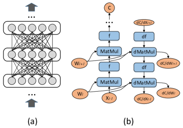
Figure 1: (a) A Multi-Layer Perceptron (MLP) model; (b) The dataflow graph of its forward and backward propagations.

⬇

for(epoch = 1 to N):

foreach ($D_{i}$ in $\{D_{1},D_{2},...\}$):

$\frac{\partial C}{\partial\theta}$ = CalculateGradient($D_{i}$, $\theta$)

$\theta:=\theta-\epsilon\frac{\partial C}{\partial\theta}$ // update model parameters

Here, the training dataset $D$ is partitioned into $batches$ $\{D_{1},D_{2},\ldots\}$ and SGD is performed iteratively, updating model parameters ($\theta$) after each batch.

DNN models have a common graphical representation, in which layers of neurons are connected by weighted edges across layers. The weights are the model parameters to be learned. DNN training involves a series of tensor computations along the graph structure. Figure 8(a) shows a Multi-Layer Perception (MLP) model with 3 fully connected layers. The weights of neuron connections between successive layers $l$ and $l+1$ are represented by matrix $W_{l}$, where $W_{l}^{i,j}$ is the weight between the i-th neuron of layer $l$ and j-th neuron of layer $l+1$. The set of weights of all layers ${W_{1},W_{2},...,W_{l}}$ is referred to as a DNN’s model parameters.

To calculate the cost function, one performs forward propagation to compute the activation of a layer from its preceding layer. Specifically, $x_{l+1}=f(x_{l}\cdot W_{l})$, where layer $l$’s activation vector $x_{l}$ is multiplied with the weight matrix $W_{l}$ and then scaled using an element-wise non-linear function $f$. The cost function is $C=g(x_{l_{out})}$ where $x_{l_{out}}$ is the activation of the last (outout) layer and $g$ is the loss function. Gradients are computed through backward propagation using the chain rule. The computation proceeds from a higher to lower layer. Specifically, two kinds of matrix computations are involved in each step. One computes the gradient of the activation $\frac{dC}{dx_{l}}=df(\frac{dC}{dx_{l+1}})W_{l}^{T}$. The other computes the gradient of weight matrix $\frac{dC}{dW_{l}}=x_{l}^{T}df(\frac{dC}{dx_{l+1}})$. Here, $df$ is the derivative function of $f$. The weight matrix $W_{l}$ is then updated using the computed gradient. Our discussion so far performs SGD on one sample only. For batched SGD on $b$ samples, the activation of each layer is represented a matrix of $b$ activation vectors.

Existing deep learning systems such as TensorFlow and MXNet offer an array-based frontend for users to express the tensor computation for the forward propagation. Because SGD is such a common computation, these systems automatically derive the computation required for the backward propagation and handle parameter updates. The overall computation for both forward and backward propagation is transformed into a dataflow graph of tensor operators. As shown in Figure 8(b), the dataflow graph for DNN training is mostly serial. Popular DNN systems such as TensorFlow and MXNet directly execute this dataflow on their backends. Hence, if a user wishes to parallelize training across devices, he or she must manually express the parallel computation in the user code so that the resulting dataflow graph generated has the required parallelism. Furthermore, users are also expected to explicitly specify placement, i.e. which device should be responsible for executing which portions of the dataflow graph. This is a tedious process.

2.2 Scaling challenges and trade-offs

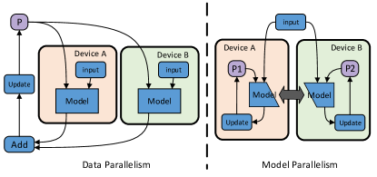
Figure 2: Data parallelism and model parallelism

Data parallelism is the widely-used method for scaling DNN training across many devices. It takes advantage of the fact that all training samples in one batch independently contribute to the gradients of the model parameters. Therefore, data parallelism partitions a batch of samples and lets each device compute the gradients of the same model parameters using a different partition. The resulting gradients are aggregated before updating the parameters. The aggregation and update can be done on each device by slicing parameters evenly, or on a separate device called a Parameter Server Li et al. [2014]; Dean et al. [2012]. After the model parameters are updated, they will be replicated to all devices for the next iteration. This results in a Bulk Synchronous Parallel (BSP) approach to parallelizing the training algorithm (Figure.2).

Data parallelism has achieved good speedup for some DNN models (e.g. Inception network Abadi et al. [2016]). However, since the communication overhead of data parallelism increases as the model grows bigger, one must train using a very large batch size to amortize the communication cost across many devices. In fact, for any DNN model, one can always scale the “training throughput” by ever increasing the batch size. Unfortunately, large batch training is known to be problematic such as longer convergence time or decreased model accuracy Krizhevsky [2014]; Keskar et al. [2016].

Model parallelism partitions the model parameters of each layer among devices, so that the update of parameters can be performed locally (Figure 2). Each device can only calculate part of a layer’s activation using its parameter partition, so all devices need to synchronize their activations and activation gradients for each layer during both the forward and backward propagations. Since model parallelism exchanges activations instead of the model parameters, it works well for models with small activation size such as DNN models with large fully-connected layers.

The trade-off between data and model parallelism can be illustrated using an example as follows. Consider a MLP network with five fully-connected layers; each layer has 300 neurons; the batch size is 400. Therefore, all weight matrices are of shape $300\times 300$ whereas activation matrices are of shape $400\times 300$ (Figure 5). The model parameter size is $300\times 300\times 5\times 4\text{B}=1.8\text{MB}$, and the total activation size of forward propagation $400\times 300\times 5\times 4\text{B}=2.4\text{MB}$. When parallelizing training for this network on 16 GPUs, data parallelism needs to first collect all parameter gradients and then synchronize the updated parameters for all devices, so the total communication is $1.8\text{MB}\times 16\times 2=57.6\text{MB}$, while model parallelism transfers activations and their gradients in both forward and backward propagations, so the total communication is $2.4\text{MB}\times 16\times 2=76.8\text{MB}$. Data parallelism is better than model parallelism in this particular example because the total activation(gradient) size is bigger than the total parameter size and data parallelism exchanges parameters across devices. If the batch size is 300 while the layer size is 400, model parallelism becomes better.

However, an even better strategy for this example is a hybrid of data and model parallelism as follows. The 16 GPUs are divided into four groups. We use data parallelism among groups, while within each group we apply model parallelism. The calculation of communication cost is then also divided into two parts. First, for data parallelism among groups, the communication is $1.8\text{MB}\times 4\times 2=14.4\text{MB}$. Second, for model parallelism within each group, the communication is $\frac{2.4}{4}\text{MB}\times 4\times 2=4.8\text{MB}$. Note that the activation size is reduced to $\frac{2.4}{4}\text{MB}$ due to data parallelism partitioning on the batch dimension. Finally, because there are four groups, the total communication is $14.4\text{MB}+4\times 4.8\text{MB}=33.6\text{MB}$. This results in communication savings of 41.7% and 56.2% compared with pure data and model parallelism, respectively.

3 Our approach

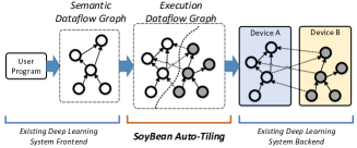
Figure 3: Overview of SoyBean’s design.

Our insight to this challenge is that data, model and hybrid parallelism can all be unified as different tensor tiling schemes including partitioning a tensor along certain dimension or replicating the whole tensor. We then find the best parallelism by finding the tensor tiling scheme that minimizes communication cost. The formulation lets us support a wide range of parallel strategies used for DNN training in the literature, including:

• Data parallelism. This corresponds to replicating the weight tensors and partitioning all other tensors by the data dimension.

• Model parallelism. This corresponds to partitioning each weight tensor along any one dimension.

• Mixed parallelism Krizhevsky [2014]. This corresponds to distributing some layers using data parallelism and other layers using some model parallelisim strategy.

• Hybrid parallelisim Dean et al. [2012]. Here, workers are divided into groups. An operator’s tensor is first partitioned across groups and then partitioned across workers within a group, using different strategies. Combined parallelism has been used by the earlier generation of specialized training systems (e.g.  Dean et al. [2012]; Chilimbi et al. [2014]), but is not explored with the current generation of general-purpose systems due to its programming complexity.

We then build a prototype system called SoyBean. Figure.3 shows an overview of SoyBean’s overall system design. We reuse the front-end of existing deep learning systems that express tensor computation by a dataflow graph, which we refer to as the semantic dataflow graph. An example semantic dataflow graph is shown in Figure 8(b). It is mostly serial. Based on the semantic dataflow graph, SoyBean determines the best tensor tiling scheme that incurs the least communication cost. SoyBean then transforms the serial semantic dataflow graph into a parallel execution dataflow graph based on the scheme. It automatically maps the partitioned arrays and operators to the set of underlying devices. Finally, the execution graph is dispatched to an existing dataflow engine backend for execution. Since the DNN training is done over many iterations using the same semantic dataflow graph, the runtime cost of the dataflow transformation can be amortized.

4 Finding the Optimal Tiling

Given a dataflow graph, SoyBean aims to find a tiling for each tensor in the graph such that the resulting parallel execution incurs minimal communication cost. There are three main challenges that SoyBean solves:

• Optimize based on the dataflow: In a dataflow graph, a tensor could act as the output of one operator as well as the input of another. Hence, a tiling that results in no communication for some operators may lead to more communications globally. For example, data parallelism requires no communication in forward and backward propagations, but the gradient aggregation part may be costly so that the overall communication cost is not minimized. SoyBean solves this by considering operators that share inputs or outputs together when searching for the optimal tiling. We also show that our algorithm could finish in polynomial time thanks to the sequential nature of deep learning algorithm.

• Determine communication cost: Given the tilings of the inputs and outputs, SoyBean needs to determine the corresponding communication costs. In SoyBean, we view communication as tiling conversions. Our core insight is that all the data needs to be fetched to the device before the operator can be executed. The process of fetching data from one location to another is in fact re-organizing the tiles and is thus equal to tiling conversion.

• Decompose the optimization problem: The problem of finding the best tiling for $n$ devices has a very large search space depending on $n$. SoyBean provides a recursive solution; it first finds the best tiling for partitioning the tensors among two devices. Then it recursively build upon its baseline solution to find tiling for $n>2$ devices.

In this section, we first discuss the formulation of the tiling problem (Sec 4.1). Next, we describe how to find the optimal tiling across two devices (Sec 4.2) and build upon this baseline solution to tile across are more than two devices (Sec 4.3). We prove the solution’s optimality in Sec 4.4 and discuss extensions in Sec 4.5.

4.1 Parallelism as the Tiling Problem

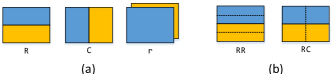
Figure 4: (a) Three basic tilings: row tiling, column tiling and replication; (b) Left: compose two basic row tilings into a four-way row tiling; right: compose row tiling and column tiling to partition matrix into four blocks.

We formulate the tiling problem to be solved by SoyBean. To ease the discussion, we only consider 2-D tensor (matrix) here. Extension to high-dimensional tensor is straight-forward and will be covered in section 4.5.

We first define the set of supported tiling schemes of a matrix. SoyBean only considers even tiling schemes that result in (sub-)tensors of the same shape and size, because we want to balance the computation across all devices. There are three basic tilings that divide a matrix computation into two equal parts: row tiling, column tiling and replication, as shown in Figure.4(a). Since all tiles are of the same shape, basic tillings can be applied again on each tile to further partition the matrix. We call this tiling composition. The result of a tiling composition is still an even tiling.

Let $T^{1}=\{\texttt{R},\texttt{C},\texttt{r}\}$ be the set that contains all basic tilings of a matrix, where R, C and r represent row tiling, column tiling and replication, respectively. We then define a $k$-cut tiling set that contains all possible tilings after $k$ compositions as follows:

Definition 1.

$T^{k}=\{t_{1}t_{2}|t_{1}\in T^{k-1}\wedge t_{2}\in T^{1}\},~{}\forall k\geqslant 2$.

For example, a 2-cut tiling set $T^{2}$ is as follows:

$$T^{2}=\{\texttt{R}\texttt{R},\texttt{R}\texttt{C},\texttt{R}\texttt{r},\texttt{C}\texttt{R},\texttt{C}\texttt{C},\texttt{C}\texttt{r},\texttt{r}\texttt{R},\texttt{r}\texttt{C},\texttt{r}\texttt{r}\}$$

Figure.4(b) shows how 2-cut tilings RR and RC partition the matrix into four pieces. Note that a $k$-cut tiling partitions a matrix into $2^{k}$ pieces. To simplify the discussion, we assume the number of workers is $n=2^{k}$.

We then formally define the tiling of a dataflow graph:

Definition 2.

The $k$-cuts tiling of a dataflow graph $G$ is a function $\mathcal{T}_{G}:M\mapsto T^{k}$ that maps from all the matrices $M$ in dataflow graph to their tilings.

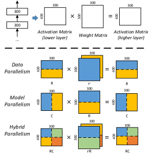
Figure 5: Top: forward propagation of one layer in a MLP model. Bottom: how matrices are tiled in the forward propagation for different parallelisms.

Given the above definition, we could unify data, model and hybrid parallelisms as different tilings of the dataflow graph (Figure.5). We explain why this is the case using the same MLP example in Figure.8.

• In data parallelism, all activations are partitioned along the batch dimension while all parameters are replicated. Suppose the batch dimension is the row dimension. Then data parallelism on two devices can be described by the following tiling:

  $$\mathcal{T}_{data}(m)=\left\{\begin{array}[]{ll}\texttt{r}&\text{if }m\text{ is weight matrix},\\ \texttt{R}&\text{otherwise.}\end{array}\right.$$

• In model parallelism, the weight matrices are partitioned in order to avoid gradient aggregation among devices. For a 2D weight matrix, there are two possible tilings: R and C. Suppose we choose row tiling. In order to compute the gradient of parameters locally, the activation matrices are partitioned along column while the activation gradients are replicated. Therefore, model parallelism on two devices can be described as following tiling:

  $$\mathcal{T}_{model}(m)=\left\{\begin{array}[]{ll}\texttt{R}&\text{if }m\text{ is weight matrix},\\ \texttt{C}&\text{if }m\text{ is activation},\\ \texttt{r}&\text{otherwise.}\end{array}\right.$$

• Hybrid parallelism divides all devices into groups. It supports one type of parallelism within a group and a different type across groups. This can be described as a composition of $\mathcal{T}_{data}$ and $\mathcal{T}_{model}$. An example tiling of hybrid parallelism on four devices is as follows. It performs data parallelism across groups and model parallelism within a group.

  $$\mathcal{T}_{hybrid}(m)=\left\{\begin{array}[]{ll}\texttt{r}\texttt{R}&\text{if }m\text{ is weight matrix},\\ \texttt{R}\texttt{C}&\text{if }m\text{ is activation},\\ \texttt{R}\texttt{r}&\text{otherwise.}\end{array}\right.$$

4.2 Tiling across two devices

We first solve the base case problem of finding the best tiling for two devices that minimizes communication. Let us consider the MLP model in Figure 8(b). If there are $L$ layers, the forward propagation for computing loss value $\mathcal{L}$ can be simplified as follows:

$$\mathcal{L}=x_{0}\prod_{1\leqslant l\leqslant L}W_{l}$$ (1)

Here, we ignore the element-wise functions. $x_{0}$ is the input data and $W_{l}$ is the weight matrix of layer $l$. How to assign the tiling schemes for all matrices in this computation to minimize the communication cost? We first explain how to calculate the communication cost of one matrix multiplication given the tilings of its input/output matrices (Sec 4.2.1). Then we give an algorithm to optimize for the cost (Sec 4.2.2).

4.2.1 Calculating the communication cost

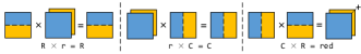
Figure 6: Three forms of aligned tilings for matrix multiplication. The resulting partition of the third form is an intermediate one red, and requires an extra reduction.

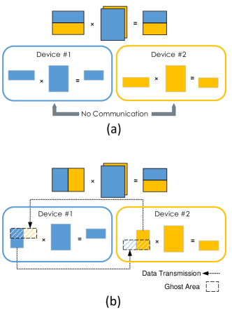
Figure 7: (a) Aligned multiplication that has no communication. (b) Unaligned multiplication. The dashed areas are “ghost areas” representing the area after tiling conversion. The yellow area on device #1 needs be fetched from device #2.

Let us first consider only one matrix multiplication, $\texttt{X}\times\texttt{Y}=\texttt{Z}$. What is the communication cost given the tilings of its inputs $t_{\texttt{X}}$ and $t_{\texttt{Y}}$ and its output $t_{\texttt{Z}}$?

This problem is a variant of the traditional block matrix multiplication, except in addition to being partitioned along rows and columns, the matrix can also be replicated. The core principle here is that each submatrix multiplication cannot be performed without all its inputs being fetched to the device on which it is executed. Therefore, we can view a parallel matrix multiplication as having three phases:

• Inputs Conversion Phase: The tiles of the inputs (X and Y) are fetched to the device(s) that require them for computation, if they reside on different devices.

• Computation Phase: Submatrix multiplications are executed on all devices locally.

• Outputs Conversion Phase: The temporary outputs of the local matrix multiplications are pushed to the devices specified by the tilings of the outputs (Z).

Notably, communication only happens in the Inputs and Outputs Conversion phases, which means we can compute the communication cost by computing the conversion costs of different tilings. However, since there are many types of input and output tilings, we do not want to enumerate all possible combinations to calculate the cost. Rather, we find a small set of so-called aligned tiling and reduce all tiling combinations to one of those cases. Aligned tilings may or may not correspond to real tilings. We use them to simplify the conversion cost calculation by drastically cutting down the number of cases we have to consider.

Given the three basic tilings, there are three corresponding aligned tilings, as depicted in Figure.6. For the left most tiling, the two inputs are row-partitioned and replicated, respectively and output is row partitioned. Similarly for the scenario in the middle. There is no communication cost for these two tilings. The third scenario is different in that its output tiling does not correspond to any basic tiling. Rather, the intermediate matrices computed on each device need to be aggregated later using an extra reduction operation. We denote this intermediate tiling as red.

All of the aligned tilings have several properties in common. First of all, they are all correct block matrix multiplications. Second, removing any submatrix product will give wrong results. Therefore, there is no redundant computation. Finally, they are balanced in that the number of submatrix products is equal to the number of devices.

One-cut Communication Cost:

Let us define $c(t_{1}{\scriptstyle\rightarrow{}}t_{2})$ as the conversion cost from tiling $t_{1}$ to $t_{2}$. To compute the communication cost of a matrix multiplication, we calculate the minimum cost of converting the given input/output tilings to one of the three aligned tilings in Figure 6. To put it formally, the communication cost $c(t_{\texttt{X}},t_{\texttt{Y}},t_{\texttt{Z}})$ of a matrix with input tiling $t_{\texttt{X}}$, $t_{\texttt{Y}}$ and output tiling $t_{\texttt{Z}}$ is as follows:

$$\min\left\{\begin{array}[]{l}c(t_{\texttt{X}}{\scriptstyle\rightarrow{}}\texttt{R})+c(t_{\texttt{Y}}{\scriptstyle\rightarrow{}}\texttt{r})+c(\texttt{R}{\scriptstyle\rightarrow{}}t_{\texttt{Z}}),\\ c(t_{\texttt{X}}{\scriptstyle\rightarrow{}}\texttt{r})+c(t_{\texttt{Y}}{\scriptstyle\rightarrow{}}\texttt{C})+c(\texttt{C}{\scriptstyle\rightarrow{}}t_{\texttt{Z}}),\\ c(t_{\texttt{X}}{\scriptstyle\rightarrow{}}\texttt{C})+c(t_{\texttt{Y}}{\scriptstyle\rightarrow{}}\texttt{R})+c(\texttt{red}{\scriptstyle\rightarrow{}}t_{\texttt{Z}})\end{array}\right\}$$ (2)

Computing the cost of tiling conversion is straightforward. It is equal to the area required for the local multiplication (which we refer to as “ghost area”) minus the area that already exists on the device. Figure 7(b) illustrates how an unaligned multiplication $\texttt{C}\times\texttt{r}=\texttt{R}$ is computed through a conversion to an aligned multiplication $\texttt{R}\times\texttt{r}=\texttt{R}$. The submatrix required for local computation is marked by the dashed line. The submatrix filled by yellow shading on device #1 needs to be fetched from device #2. Hence, its area is equal to the amount of communications involved in this tiling conversion.

4.2.2 One-cut tiling algorithm

Given a dataflow graph $G$, the one-cut tiling algorithm finds a tiling across two devices (or groups), $\mathcal{T}_{min}:M\mapsto T^{1}$, such that the overall communication cost is minimized:

$$\mathcal{T}_{min}=\operatorname*{arg\,min}_{\mathcal{T}}\sum_{o\in O_{G}}c(\mathcal{T}(o_{\texttt{X}}),\mathcal{T}(o_{\texttt{Y}}),\mathcal{T}(o_{\texttt{Z}}))$$ (3)

where $O_{G}$ represents all the matrix multiplications in the dataflow graph $G$, and $o_{\texttt{X}}$, $o_{\texttt{Y}}$ and $o_{\texttt{Z}}$ represent the input matrices and output matrix of a matrix multiplication $o$.

The central problem in searching optimal tilings is that changing the tiling of one matrix may affect many multiplications. Again, let us look at the MLP example. If we only consider the forward propagation part $\mathcal{L}=x_{0}\prod_{1\leqslant l\leqslant L}W_{l}$, we can first calculate the communication cost of $x_{1}=x_{0}W_{1}$ under all the possible tilings of $x_{0}$, $x_{1}$ and $W_{1}$. We then proceed to the next multiplication $x_{2}=x_{1}W_{2}$, but when choosing $x_{1}$ to be tiling $t_{1}$, we should include the minimal cost of $x_{1}$ to be $t_{1}$ in the first multiplication. The total communication cost is then the minimal cost after we finish the last multiplication. When further taking the backward propagation part $\frac{d\mathcal{L}}{dx_{0}}=\frac{d\mathcal{L}}{dx_{L}}\prod_{L\geqslant l\geqslant 1}W_{l}^{T}$ into consideration, two multiplications ($x_{l}=x_{l-1}W_{l}$ and $\frac{d\mathcal{L}}{dx_{l-1}}=\frac{d\mathcal{L}}{dx_{l}}W_{l}^{T}$) should be considered together, because the tiling of $W_{l}$ affects both multiplications.

Our tiling algorithm exploits an intuitive idea: operators that share inputs or outputs should be considered together. To achieve this, our algorithm first treats the dataflow graph as an undirected graph $G^{\prime}$, and then uses a breadth-first search on this graph to organize graph nodes into a list of levels $L=\langle l_{0},l_{1},\ldots,l_{n}\rangle$. BFS puts nodes that share inputs or outputs in adjacent levels. We then use dynamic programming (DP) to search for optimal tilings:

Initial condition:

$$g_{0}(\tau_{0})=\text{level\_cost}_{0}(\phi,\tau_{0})$$ (4)

DP equation ($l\geqslant 1$):

$$g_{l}(\tau_{l})=\min_{\tau_{l-1}}\left\{\text{level\_cost}_{l}(\tau_{l-1},\tau_{l})+g_{l-1}(\tau_{l-1})\right\}$$ (5)

Here, $\tau_{l}$ contains the tilings of all matrices that are shared among multiplications in level $l$ and $l+1$. The $\text{level\_cost}_{l}$ is calculated by summing up the cost of each matrix multiplication in level $l$. The DP state $g_{l}(\tau_{l})$ represents the minimal communication cost after executing all the operators from level zero to level $l$ and also partitioning matrices used by level $l+1$ by tilings in $\tau_{l}$.

The algorithm searches for all possible tilings and therefore guarantees optimal. Unfortunately, the running time of the DP algorithm is exponential. Because all the operations are matrix multiplications, the node degree in the undirected graph $G^{\prime}$ is at most three. According to Moore bound, if there are $N$ nodes in the graph, the diameter is $O(\log N)$. Since the number of BFS levels is equal to the graph diameter, the maximum number of nodes in each level is $O(N/logN)$. Computing the total cost of each level needs to explore all tiling combinations of the inputs and outputs of the operators in that level. Therefore, the worst-case complexity of calculating $\text{level\_cost}_{l}$ is $|T^{1}|^{O(N/\log N)}=O(3^{N})$.

The observation that saves us is that deep learning does not have an arbitrary dataflow graph. Rather, its graph usually has a large diameter. This is because training neural network usually involves computing each layer sequentially. For an $N$-layer MLP network, there are $3N$ matrix multiplications (forward, backward and gradient computation) and the diameter is $N$. In this case, the average number of nodes in each level is some constant $c$, so the average running complexity of the whole DP algorithm is linear, $O(3^{c}N)$.

4.3 Tiling across many devices

The $k$-cut algorithm finds the optimal tiling for $n=2^{k}$ devices. It is a recursive algorithm. Specifically, we can divide $2^{k}$ devices into 2 groups, each with $2^{k-1}$ devices. We first use the one-cut algorithm to find the best tiling to partition the computation among the two groups. Within each group, we perform $(k-1)$-cuts to find the optimal tiling. Algorithm 1 shows the pseudocode.

input : A dataflow graph $G$ and a number $k$

output : A $k$-cuts tiling $\mathcal{T}$ of the graph and its communication cost $c$

if $k=0$ then

      return $\phi$ and $0$

else

       $\mathcal{P}_{k}$, $\delta_{k}$ $\leftarrow$ OneCutTiling($G$);

       $G^{\prime}$ $\leftarrow$ ConstructTileGraph($G$, $\mathcal{P}_{k}$);

       $\mathcal{T}_{k-1}$, $c_{k-1}$ $\leftarrow$ KCutsTiling($G^{\prime}$, $k-1$);

       $\mathcal{T}_{k}$ $\leftarrow$ $\mathcal{P}_{k}\circ\mathcal{T}_{k-1}$;

       $c_{k}$ $\leftarrow$ $\delta_{k}+2c_{k-1}$;

       return $\mathcal{T}_{k}$ and $c_{k}$

Algorithm 1 $k$-cuts tiling algorithm

In Algorithm 1, $\mathcal{P}_{k}\circ\mathcal{T}_{k-1}$ is the composition of two tilings (see Section 4.1). $\delta_{k}$ is the cost of the $k$-th cut. As each cut partitions computation into two groups, the cost of the subproblem is multiplied by two. The total communication cost is the weighted summation of per-cut costs:

Theorem 1 (Total communication cost).

$c_{k}=\sum_{i=1}^{k}2^{k-i}\delta_{i}$

4.4 Proof of Optimality

Due to the limit of space, we only emphasize the key point that leads our proof. The core property that makes the $k$-cuts algorithm optimal is the commutativity of tiling composition because they are orthogonal ways of partitioning. If we let $\texttt{R}^{k}$ be the $k$-row tiling, then the $T^{2}$ tiling set could be rewritten as $T^{2}=\{\texttt{R}^{2},\texttt{C}^{2},\texttt{r}^{2},\texttt{R}\texttt{C},\texttt{R}\texttt{r},\texttt{C}\texttt{r}\}$. In fact, we have:

Theorem 2 (Flattening).

$$T^{k}=\{\texttt{R}^{k_{\texttt{R}}}\texttt{C}^{k_{\texttt{C}}}\texttt{r}^{k_{\texttt{r}}}|k_{\texttt{R}},k_{\texttt{C}},k_{\texttt{r}}\in\mathbb{Z}\wedge k_{\texttt{R}}+k_{\texttt{C}}+k_{\texttt{r}}=k\}$$

Let $\mathcal{T}_{k}=\langle\mathcal{P}_{k},\mathcal{P}_{k-1},\ldots,\mathcal{P}_{1}\rangle$ be the tiling sequence generated by our $k$-cuts algorithm. We can also prove that the order of the tiling applied will not influence the total communication cost $c_{k}$. This gives us the following property:

Theorem 3 (Greediness).

Let $\delta_{k},\delta_{k-1},\ldots\delta_{1}$ be the cost of each tiling. We have $\delta_{i}\leqslant 2\delta_{i-1},~{}\forall 2\leqslant i\leqslant k$.

The greedy theorem means that for any tiling sequence $\mathcal{T}_{k}$ we can reorder it such that the contribution of the cost of each tiling is increasing. Suppose there is another tiling sequence $\mathcal{T}_{k}^{\prime}$ that is not chosen by our algorithm but has $c_{k}^{\prime}<c_{k}$, we can prove that there must exist a “cross” step such that after that step, the remaining tilings in $\mathcal{T}_{k}$ produces larger communication cost than the remaining tilings in $\mathcal{T}_{k}^{\prime}$. We can prove that by choosing the tiling at the “cross” step in $\mathcal{T}_{k}^{\prime}$, it will give smaller cost than the one in $\mathcal{T}_{k}$ which contradicts to the local optimality of $k$-cuts algorithm.

4.5 Extensions to General Dataflow Graph

First, we extend the $k$-cuts tiling algorithm to high-dimensional tensors. We change the basic tiling set to $T^{1}=\{\texttt{P}_{1},\texttt{P}_{2},\ldots,\texttt{P}_{d},\texttt{r}\}$, where $\texttt{P}_{d}$ represents partitioning along $d^{th}$ dimension. The running complexity of the one-cut algorithm then becomes $O((d+1)^{c}N)$ given $N$ nodes in the dataflow graph, which is still acceptable provided that $d$ is usually small.

Second, we discuss how to handle operators beyond matrix multiplications. Recall that the communication cost is equal to the tiling conversion cost. The only information that is tied to operator type is the set of the aligned tilings of an operator. Here, we categorize operators for discussion. For element-wise functions (e.g. non-linear activation function), the only aligned computation method is to have the same tiling for all of the operator’s inputs and outputs. Note that having all of an operator’s inputs and outputs replicated is not allowed due to redundant computation. For convolution, the activation and parameter tensors have four dimensions. Tiling on batch dimension leads to data parallelism while tiling on channel dimensions leads to model parallelism. Tilings on image and kernel dimensions are strictly worse than data parallelism so is ignored in our implementation. Note that the image and kernel sizes are in fact multipliers on the batch size and weight size, respectively. The larger the image size, the larger the activation tensor and thus the better data parallelism is. Finally, for all other operators, we only allow partitioning on the batch dimension, resulting in data parallelism. These changes should be easy since they only focus on the operator semantics while the complicated communication patterns will be automatically deduced by SoyBean.

5 Constructing the Execution Dataflow Graph

This section covers how SoyBean dispatches operators to different devices and how the semantic dataflow graph is converted to the execution graph given the $k$-cuts tiling schemes computed by our algorithm.

5.1 Tile Placement

The first consideration is load balancing. Fortunately, SoyBean’s tiling algorithm ensures that all tensors and operators in the dataflow graph are evenly partitioned, which means the workload is perfectly balanced.

Another consideration is the interconnects between devices. For example, GPUs within a single machine can be connected to different CPUs by PCI-e. Given the fixed total amount of communications, we want the majority of data transmission to be between GPUs attached to the same CPU to avoid the high latency of QPI connections. When scaling beyond one machine, this becomes more critical since network transmission is even slower. At a high level, the interconnection hierarchy divides devices into groups and encourages communications within each group. The $k$-cuts tiling algorithm naturally fits this scenario because each cut partitions the workload into two groups of devices; each group is then recursively partitioned. Theorem 3 indicates that SoyBean tends to partition groups such that the majority of communication happens within groups. Therefore, our placement strategy follows the algorithm structure. We map the workloads partitioned by the first cut to the groups connected by the slowest interconnects (e.g. Ethernet or QPI). We then continue mapping workloads within each group to the second slowest interconnects, and so on.

5.2 Connecting Partitioned Operators

The $k$-cuts tiling algorithm partitions each operator in the semantic graph into $2^{k}$ sub-operators. The inputs and outputs of these sub-operators are tiles (sub-tensors) of their original inputs and outputs. Therefore, to construct the execution graph is to connect the sub-operators for every connected operators in the semantic graph. Similar to the aligned matrix multiplication, this includes three phases:

1. We need to first convert the input tiling to the aligned tiling for the downstream operator. The tiling conversion dispatches each tile to the location specified by the placement. A simple solution is letting the receiver devices pull from the device that contains the area they need. The situation becomes complicated when the receiver only needs one slice of the sender’s data and needs to concatenate slices from multiple senders. In this case, we transfer the data in three steps. First, the flattening theorem (Theorem 2) allows us to represent each original tensor as a grid of tiles. Therefore, the sender can slice its own tile into shards such that each shard is dispatched to different receiver. Second, the receivers will fetch the shards they need from senders. Finally, the flattening theorem again allows the receiver to directly concatenate the received shards back to tiles.

2. Once the tiling conversions of inputs are done, all sub-operators can be executed locally by the definition of aligned tiling. Moreover, since all sub-operators are identical, we can just connect the input tiles to the sub-operators one by one.

3. The temporary outputs of the sub-operators again should be converted to the output tilings for later computation. This is the same process as the input tiling conversion.

6 Evaluation

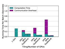
(a) Batch size = 512; Hidden Size = 8K

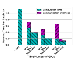
(b) Batch size = 2K; Hidden Size = 8K

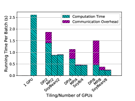
(c) Batch size = 2K; Hidden Size = 12K

Figure 8: Runtime comparison of a 4-layer MLP for DP, MP, and SoyBean with different batch sizes and hidden sizes.  

In this section, we examine SoyBean’s performance. Specifically, we want to answer following questions:

1. Is communication really a bottleneck when using data parallelism with small batch sizes?

2. Can SoyBean reduce overall runtime?

3. How well does SoyBean accelerate modern DNNs?

6.1 Experimental Setup

We evaluated SoyBean on Amazon’s EC2 cluster. We used a p2.8xlarge instance, with 480GB of memory and 32 virtual CPUs as well as 8 NVIDIA GK210 GPUs on the instance. Each of the GPUs has 12GB of memory; they are connected by PCI-e, with a maximum peer-to-peer bi-directional bandwidth of 20GB/s.

6.2 Communication Overhead Evaluation

In this evaluation, we want to know if communication overhead accounts for a large percentage of the overall runtime when the batch size is relatively small or when the weight size is large. We first tested the runtime for data parallelism (DP), model parallelism (MP), and SoyBean with different parameters, i.e., batch size and weight size. To see the ratio of the communication overhead to runtime, we also modified MXNet’s backend to skip any communication, and re-ran our experiments. Thus, the runtime measured by the modified backend is solely due to computation. We can then determine the communication overhead by subtracting the computation time from the original runtime. Note that we report communication overhead instead of communication time because communication can be overlapped with computation. As a result, the communication overhead is strictly smaller than the communication time.

Figure 8(a) and Figure 8(b) show the runtime and communication overhead of a 4-layer MLP for different tilings on different numbers of GPUs. Both tests have the same weight size, 8192$\times$8192, but different batch sizes, 512 and 2048, respectively. In Figure 8(a), the communication overhead for data parallelism increases as the number of GPUs increases. This is because a GPU needs to send its data to more GPUs when the total number of GPUs increases. However, the aggregate communication throughput is limited by contention on shared PCI-e resources, so it cannot increase linearly with several simultaneous peer-to-peer connections. As a result, increased GPU-to-GPU communication is slower, even below the PCI-e bandwidth limit.

In these two figures, data parallelism performs sq worse than MP and SoyBean. That’s because both communication overhead and computation time in data parallelism are larger than MP and SoyBean. We will show why different tilings may result in different computation time in Section 6.3. However, even if the computation time is the same as with MP and/or SoyBean, data parallelism is still slower. The key reason is the communication overhead is huge, $\scriptstyle\mathtt{\sim}$5$\times$ longer than the computation time on 8 GPUs with batch size 512, and $\scriptstyle\mathtt{\sim}$2.5$\times$ longer on 8 GPUs with batch size 2048.

Figure 8(c) uses the same batch size as Figure 8(b) but with larger weight size, 12288 (12K). Unlike changing the batch size, which significantly affects the ratio of communication overhead to total runtime, changing the weight size from 8K to 12K has little effect on the ratio. This is because when changing the weight size, both communication and computation increase for all parallelism schemes.

The results show that to achieve good performance, one should not use data parallelism when the batch size is small, due to the communication overhead. As the batch size increases, the percentage of the runtime consumed by communication overhead becomes smaller for data parallelism, and a crossover point will be reached when its runtime is lower than model parallelism on the same model and batch size. Because SoyBean can use hybrid tilings, it always achieves optimally low communication overhead.

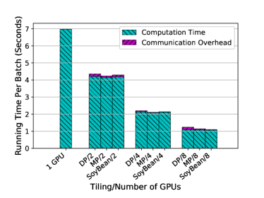
(a) Image Size = 6x6, Filter Size = 2048

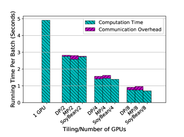
(b) Image Size = 24x24, Filter Size = 512

Figure 9: Runtime comparison of training a 5-layer convolutional neural network using DP, MP, and SoyBean. The batch size is 256.  

We also performed the same evaluation for convolution neural networks. Figure 9(a) shows results from training a CNN with small (6px$\times$6px) images with a large filter size (2K), while Figure 9(b) shows results from training with larger (24px$\times$24px) images with a small filter size (512). We fixed the batch size to 256 for both experiments. The results show that with the larger image size, data parallelism has better performance than model parallelism. SoyBean still outperforms both partitioning schemes due to its ability to cut in different dimensions.

6.3 Can Shape Affect Computation Performance?

Batch Size	Single GPU	Single GPU w/ SoyBean tilings
512	0.31s	0.19s
1024	0.56s	0.39s
2048	1.13s	0.73s

Table 1: Runtime per batch comparison for a 4-layers MLP network between single GPU and single GPU with SoyBean partitions. The weight size is fixed to 8K$\times$8K.

Figure 8 shows that the computation time varies with the tiling approach chosen. Regardless of the tiling, however, the total amount of computed data is the same. Therefore, we suspected that the shapes of matrices might affect the computation performance. To validate this assumption, we partitioned the input matrices into several sub-matrices by using SoyBean, but put all of them on single GPU. We achieved better performance with this approach than with using the un-cut matrices to do the same computation on a single GPU, as shown in table 1. We believe the difference is related to how CUDA Nickolls et al. [2008] chooses different algorithms according to the matrix shapes.

6.4 Scalability

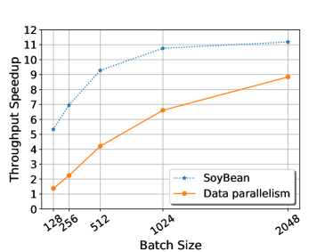
(a) AlexNet throughput speedup.

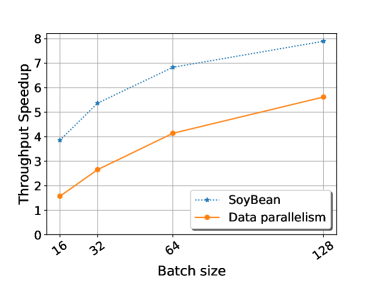
(b) VGG throughput speedup.

Figure 10: Throughtput comparison of SoyBean and data parallelism on 8 GPUs.  

Our goal is to achieve good performance regardless of the model and batch sizes; particularly difficult is good scalability with smaller batch sizes, which data parallelism does not achieve. In this section, we evaluate SoyBean’s scalability with two popular image recognition neural networks, AlexNet and VGG on 8 GPUs. We first trained each network on a single GPU to determine the maximum throughput (images/second). Using this throughput as baseline, we then calculated the speedup for different batch sizes.

Figure 10(a) shows the results with AlexNet. SoyBean achieves a greater than $7\times$ speedup with a batch size of 256, while data parallelism requires increasing the batch size to more than 1K to achieve the same speedup. AlexNet consists of many convolution layers followed by fully connected layers. As discussed in Section 6.2, data parallelism needs a large batch size to achieve good scalability for fully connected layers. Moreover, Section 6.2 also shows that SoyBean can always achieve similar or better performance for convolution layers than data parallelism. As a result, SoyBean performs much better than data parallelism. VGG has similar structure to AlexNet but with more layers. Therefore, SoyBean can still achieve better scalability than data parallelism as shown in Figure 10(b). One may notice that in Figure 10(a), SoyBean can achieve superlinear speedup. This is because some matrix shapes fall into categories that have better computation performance after partitioning, as discussed in Section 6.3.

7 Related Work

How to distribute arbitrary data easily for users while achieving high-performance computation at the same time has been a popular research topic. However, it is difficult to design systems that automatically optimizes locality without knowledge of the underlying data and processing. Relatedly, distributed array programs are increasingly important due to the emergence of machine learning and deep learning. As a result, significant effort has been expended in optimizing distributed array frameworks.

Deep learning systems. Many frameworks, such as Tensorflow Abadi et al. [2016], MXNet Chen et al. [2015], PyTorch pyt , Theano Bergstra et al. [2010] and Caffe2 Facebook [2017] have been proposed to facilitate developing new neural network models. These distributed array frameworks emphasize deep learning and machine learning applications. Besides the common array operations, they also provide many functionalities for neural networks such as automatic differentiation (backpropagation).

Though these frameworks allow users to develop models with both data parallelism and model parallelism, their interfaces are not friendly for utilizing model parallelism. SoyBean not only simplifies exploit model parallelism, but can automatically choose correct combinations of various parallelisms to reduce communication. Moreover, because of the similar design approach, performing optimizations over data-flow graphs, SoyBean can be implemented in these frameworks as long as they allow customized optimizations.

General distributed programming frameworks. Most distributed frameworks target primitives for key-value collections (e.g. MapReduce Dean and Ghemawat [2004], Dryad Isard et al. [2007], Piccolo Power and Li [2010], Spark Zaharia et al. [2010], Ciel Murray et al. [2011], Dandelion Rossbach et al. [2013] and Naiad Murray et al. [2013]). Some provide graph-centric primitives (e.g. GraphLab Low et al. [2012] and Pregel Malewicz et al. ). It is possible to implement a deep learning framework backend by augmenting an in-memory framework, such as Spark or Piccolo. When doing so, SoyBean can be applied to optimize the high-level data-flow graph before lowering the graph to the underlying framework.

Distributed array frameworks. Relational queries are a natural layer on top of key-value centric distributed execution frameworks, as seen in systems like DryadLINQ Yu et al. [2008], Shark Xin et al. [2013], Dandelion Rossbach et al. [2013] and Dremel Melnik et al. [2010]. Several attempts have been made to build array interfaces on these. MadLINQ Qian et al. [2012] adds support for distributed arrays and array-style computation to the dataflow model of DryadLINQ Yu et al. [2008]. SciHadoop Buck et al. [2011] is a plug-in for Hadoop to process array-formatted data. Google’s R extensions Stokely et al. [2011], Presto Venkataraman et al. [2013] and SparkR spa extend the R language to support distributed arrays. Julia Jul is a newly developed dynamic language designed for high performance and scientific computing. Julia provides primitives for users to parallel loops and distribute arrays. Theoretically, one can use these extensions and languages to implement any neural network models. However, users have to manually deal with all optimizations provided by deep learning frameworks, like backpropagation (and with SoyBean, tiling).

Spartan Huang et al. [2015] and Kasen Zhang et al. [2016] are two distributed array frameworks that perform automatic tiling on general array programs. Both systems provide primitives operating directly on arrays and thus expose the data access pattern of array operations that can be used for tiling optimization. Spartan proves that under such setting, automatic tiling is an NP-hard problem and provides only heuristic algorithms to find the best tiling. By contrast, SoyBean specifically targets deep learning systems and observes many fixed graph structures in neural network models. These fixed graph structures allow SoyBean to be able to find the optimal solutions in most cases. Moreover, SoyBean doesn’t rely on specific primitives, but directly optimizes array operations.

Distributed array libraries. Optimized, distributed linear algebra libraries, like LAPACK Anderson et al. [1990], ScaLAPACK Choi et al. [1992], Elemental Poulson et al. [2013] Global Arrays Toolkit Nieplocha et al. [1996] and Petsc Balay et al. [2014, 1997] expose APIs specifically designed for large matrix operations. They focus on providing highly optimized implementations of specific operations. However, their speed depends on correct partitioning of arrays and their programming models are difficult for use in deep learning.

Compiler-assisted data distribution. Prior work in this space proposes static, compile-time techniques for analysis. The first set of techniques focuses on partitioning Hudak and Abraham [1990]; the second on data co-location Knobe et al. [1990]; Philippsen [1995]; Milosavljevic and Jabri [1999]. Prior work also has examined nested loops with affine array subscript patterns, using different structures (vector Hudak and Abraham [1990], matrix Ramanujam and Sadayappan [1991] or reference Ju and Dietz [1992]) to model memory access patterns or polyhedral model Lu et al. [2009] to perform localization analysis. Since static analysis deals poorly with ambiguities in source code Anderson [2008], recent work proposes profile-guided methods Chu et al. [2007] and memory-tracing Park et al. [2014] to capture memory access patterns. Simpler approaches focus on examining stencil code Park et al. [2014]; He et al. [2011]; Hernandez [2013]; Kessler [1996]; Henretty et al. [2011].

Access patterns can be used to find a distribution of data that minimizes communication cost Hudak and Abraham [1990]; Ramanujam and Sadayappan [1989]; Bau et al. [1995]; D’HOLLANDER [1989]; Huang and Sadayappan [1993]. All approaches construct a weighted graph that captures possible layouts. Although searching the optimal solution is NP-Complete Kennedy and Kremer [1998]; Kremer [1993]; Li and Chen [1990, 1991], heuristics perform well in practice Li and Chen [1991]; Philippsen [1995]. DMLL Brown et al. [2016] aims to extend a data-parallel programming mode to heterogeneous hardware. To achieve the goal, DMLL propose a new intermedia language based on common parallel patterns to partition data and distributed across the underlying heterogeneous distributed hardware.

SoyBean borrows many ideas from these works, such as constructing a weighted graph. However, unlike prior work that requires language-specific extensions and/or modification to capture parallel access patterns, SoyBean is designed to utilize the parallelism exposed by the underlying data-flow graphs, and can be quickly integrated with modern deep learning frameworks.

8 Conclusion

Deep learning systems have become indispensible in many fields, but as their complexities grow, DNN training time is becoming increasingly intractable. We demonstrate effective tiling in SoyBean that can achieve performance as good as or better than the best of data parallelism and model parallelism for many types of DNNs on multiple GPUs. With the speed and simplicity provided by SoyBean’s backend, users can train networks using frontends like TensorFlow and MXNet quickly and easily, making DNNs useful for a larger audience.

References

- [1] Julia language. http://julialang.org.
- [2] PyTorch. http://pytorch.org.
- [3] Sparkr: R frontend for spark. http://amplab-extras.github.io/SparkR-pkg.
- Abadi et al. [2016] M. Abadi, P. Barham, J. Chen, Z. Chen, A. Davis, J. Dean, M. Devin, S. Ghemawat, G. Irving, M. Isard, M. Kudlur, J. Levenberg, R. Monga, S. Moore, D. G. Murray, B. Steiner, P. Tucker, V. Vasudevan, P. Warden, M. Wicke, Y. Yu, and X. Zheng. Tensorflow: A system for large-scale machine learning. In 12th USENIX Symposium on Operating Systems Design and Implementation (OSDI 16), 2016.
- Anderson et al. [1990] E. Anderson, Z. Bai, J. Dongarra, A. Greenbaum, A. McKenney, J. Du Croz, S. Hammerling, J. Demmel, C. Bischof, and D. Sorensen. LAPACK: A portable linear algebra library for high-performance computers. In Proceedings of the 1990 ACM/IEEE conference on Supercomputing, pages 2–11. IEEE Computer Society Press, 1990.
- Anderson [2008] P. Anderson. The use and limitations of static-analysis tools to improve software quality. CrossTalk: The Journal of Defense Software Engineering, 21(6):18–21, 2008.
- Balay et al. [1997] S. Balay, W. D. Gropp, L. C. McInnes, and B. F. Smith. Efficient management of parallelism in object oriented numerical software libraries. In E. Arge, A. M. Bruaset, and H. P. Langtangen, editors, Modern Software Tools in Scientific Computing, pages 163–202. Birkhäuser Press, 1997.
- Balay et al. [2014] S. Balay, S. Abhyankar, M. F. Adams, J. Brown, P. Brune, K. Buschelman, V. Eijkhout, W. D. Gropp, D. Kaushik, M. G. Knepley, L. C. McInnes, K. Rupp, B. F. Smith, and H. Zhang. PETSc users manual. Technical Report ANL-95/11 - Revision 3.5, Argonne National Laboratory, 2014.
- Bau et al. [1995] D. Bau, I. Kodukula, V. Kotlyar, K. Pingali, and P. Stodghill. Solving alignment using elementary linear algebra. In Languages and Compilers for Parallel Computing, pages 46–60. Springer, 1995.
- Bergstra et al. [2010] J. Bergstra, O. Breuleux, F. Bastien, P. Lamblin, R. Pascanu, G. Desjardins, J. Turian, D. Warde-Farley, and Y. Bengio. Theano: a CPU and GPU math expression compiler. In Proceedings of the Python for Scientific Computing Conference (SciPy), 2010.
- Brown et al. [2016] K. J. Brown, H. Lee, T. Rompf, A. K. Sujeeth, C. De Sa, C. Aberger, and K. Olukotun. Have abstraction and eat performance, too: Optimized heterogeneous computing with parallel patterns. In Proceedings of the 2016 International Symposium on Code Generation and Optimization, CGO ’16, 2016.
- Buck et al. [2011] J. B. Buck, N. Watkins, J. LeFevre, K. Ioannidou, C. Maltzahn, N. Polyzotis, and S. Brandt. Scihadoop: array-based query processing in hadoop. In Proceedings of 2011 International Conference for High Performance Computing, Networking, Storage and Analysis, 2011.
- Chen et al. [2015] T. Chen, M. Li, Y. Li, M. Lin, N. Wang, M. Wang, T. Xiao, B. Xu, C. Zhang, and Z. Zhang. MXNet: A Flexible and Efficient Machine Learning Library for Heterogeneous Distributed Systems. ArXiv e-prints, Dec. 2015.
- Chilimbi et al. [2014] T. Chilimbi, Y. Suzue, J. Apacible, and K. Kalyanaraman. Project adam: Building an efficient and scalable deep learning training system. In Proceedings of the 11th USENIX Conference on Operating Systems Design and Implementation, OSDI’14, 2014.
- Cho et al. [2014] K. Cho, B. van Merrienboer, C. Gulcehre, F. Bougares, H. Schwenk, and Y. Bengio. Learning phrase representations using RNN encoder-decoder for statistical machine translation. 2014.
- Choi et al. [1992] J. Choi, J. J. Dongarra, R. Pozo, and D. W. Walker. Scalapack: A scalable linear algebra library for distributed memory concurrent computers. In Frontiers of Massively Parallel Computation, 1992., Fourth Symposium on the, pages 120–127. IEEE, 1992.
- Chu et al. [2007] M. Chu, R. Ravindran, and S. Mahlke. Data access partitioning for fine-grain parallelism on multicore architectures. In Microarchitecture, 2007. MICRO 2007. 40th Annual IEEE/ACM International Symposium on, pages 369–380. IEEE, 2007.
- Dahl et al. [2011] G. Dahl, D. Yu, L. Deng, and A. Acero. Context-dependent pre-trained deep neural networks for large vocabulary speech recognition. In IEEE Transactions on Audio, Speech, and Language Processing, 2011.
- Dean and Ghemawat [2004] J. Dean and S. Ghemawat. Mapreduce: Simplified data processing on large clusters. In Symposium on Operating System Design and Implementation (OSDI), 2004.
- Dean et al. [2012] J. Dean, G. S. Corrado, R. Monga, K. Chen, M. Devin, Q. V. Le, M. Z. Mao, M. Ranzato, A. Senior, P. Tucker, K. Yang, and A. Y. Ng. Large scale distributed deep networks. In Neural Information Processing Systems (NIPS), 2012.
- D’HOLLANDER [1989] E. D’HOLLANDER. Partitioning and labeling of index sets in do loops with constant dependence vectors. In 1989 International Conference on Parallel Processing, University Park, PA, 1989.
- Facebook [2017] Facebook. Caffe2: a lightweight, modular, and scalable deep learning framework, 2017. URL https://github.com/caffe2/caffe2.
- He et al. [2011] J. He, A. E. Snavely, R. F. Van der Wijngaart, and M. A. Frumkin. Automatic recognition of performance idioms in scientific applications. In Parallel & Distributed Processing Symposium (IPDPS), 2011 IEEE International, pages 118–127. IEEE, 2011.
- Henretty et al. [2011] T. Henretty, K. Stock, L.-N. Pouchet, F. Franchetti, J. Ramanujam, and P. Sadayappan. Data layout transformation for stencil computations on short-vector simd architectures. In Compiler Construction, pages 225–245. Springer, 2011.
- Hernandez [2013] C. K. O. Hernandez. Open64-based regular stencil shape recognition in hercules. 2013.
- Hinton et al. [2012] G. Hinton, L. Deng, D. Yu, G. Dahl, A. rahman Mohamed, N. Jaitly, A. Senior, V. Vanhoucke, P. Nguyen, T. Sainath, and B. Kingsbury. Deep neural networks for acoustic modeling in speech recognition. Signal Processing Magazine, 2012.
- Huang et al. [2015] C.-C. Huang, Q. Chen, Z. Wang, R. Power, J. Ortiz, J. Li, and Z. Xiao. Spartan: A distributed array framework with smart tiling. In USENIX Annual Technical Conference, 2015.
- Huang and Sadayappan [1993] C.-H. Huang and P. Sadayappan. Communication-free hyperplane partitioning of nested loops. Journal of Parallel and Distributed Computing, 19(2):90–102, 1993.
- Hudak and Abraham [1990] D. E. Hudak and S. G. Abraham. Compiler techniques for data partitioning of sequentially iterated parallel loops. In ACM SIGARCH Computer Architecture News, volume 18, pages 187–200. ACM, 1990.
- Ilya Sutskever [2014] Q. L. Ilya Sutskever, Oriol Vinyals. Sequence to sequence learning with neural network. In Advances in Neural Information Processing Systems (NIPS), 2014.
- Isard et al. [2007] M. Isard, M. Budiu, Y. Yu, A. Birrell, and D. Fetterly. Dryad: Distributed data-parallel programs from sequential building blocks. In European Conference on Computer Systems (EuroSys), 2007.
- Ju and Dietz [1992] Y.-J. Ju and H. Dietz. Reduction of cache coherence overhead by compiler data layout and loop transformation. In Languages and Compilers for Parallel Computing, pages 344–358. Springer, 1992.
- K. Simonyan [2015] A. Z. K. Simonyan. Very deep convolutional networks for large-scale image recognition. In International Conference on Learning Representations, 2015.
- Kennedy and Kremer [1998] K. Kennedy and U. Kremer. Automatic data layout for distributed-memory machines. ACM Transactions on Programming Languages and Systems (TOPLAS), 20(4):869–916, 1998.
- Keskar et al. [2016] N. S. Keskar, D. Mudigere, J. Nocedal, M. Smelyanskiy, and P. T. P. Tang. On large-batch training for deep learning: Generalization gap and sharp minima. In arXiv:1609.04836, 2016.
- Kessler [1996] C. W. Kessler. Pattern-driven automatic parallelization. Scientific Programming, 5(3):251–274, 1996.
- Knobe et al. [1990] K. Knobe, J. D. Lukas, and G. L. Steele Jr. Data optimization: Allocation of arrays to reduce communication on simd machines. Journal of Parallel and Distributed Computing, 8(2):102–118, 1990.
- Kremer [1993] U. Kremer. Np-completeness of dynamic remapping. In Proceedings of the Fourth Workshop on Compilers for Parallel Computers, Delft, The Netherlands, 1993.
- Krizhevsky [2014] A. Krizhevsky. One weird trick for parallelizing convolutional neural networks. In arXiv:1404.5997, 2014.
- Krizhevsky et al. [2012] A. Krizhevsky, I. Sutskever, and G. Hinton. Imagenet classification with deep convolutional neural networks. In Advances in Neural Information Processing Systems 25, pages 1106–1114, 2012.
- Li and Chen [1990] J. Li and M. Chen. Index domain alignment: Minimizing cost of cross-referencing between distributed arrays. In Frontiers of Massively Parallel Computation, 1990. Proceedings., 3rd Symposium on the, pages 424–433. IEEE, 1990.
- Li and Chen [1991] J. Li and M. Chen. The data alignment phase in compiling programs for distributed-memory machines. Journal of parallel and distributed computing, 13(2):213–221, 1991.
- Li et al. [2014] M. Li, D. G. Andersen, J. W. Park, A. J. Smola, A. Ahmed, V. Josifovski, J. Long, E. J. Shekita, and B.-Y. Su. Scaling distributed machine learning with the parameter server. In USENIX OSDI, 2014.
- Low et al. [2012] Y. Low, J. Gonzalez, A. Kyrola, D. Bickson, C. Guestrin, and J. Hellerstein. Graphlab: A new parallel framework for machine learning. In Conference on Uncertainty in Artificial Intelligence (UAI), 2012.
- Lu et al. [2009] Q. Lu, C. Alias, U. Bondhugula, T. Henretty, S. Krishnamoorthy, J. Ramanujam, A. Rountev, P. Sadayappan, Y. Chen, H. Lin, et al. Data layout transformation for enhancing data locality on nuca chip multiprocessors. In Parallel Architectures and Compilation Techniques, 2009. PACT’09. 18th International Conference on, pages 348–357. IEEE, 2009.
- [46] A. L. Maas, A. Y. Hannun, C. T. Lengerich, P. Qi, D. Jurafsky, and A. Y. Ng. Increasing deep neural network acoustic model size for large vocabulary continuous speech recognition. CoRR, abs/1406.7806.
- [47] G. Malewicz, M. H. Austern, A. J. Bik, J. C. Dehnert, I. Horn, N. Leiser, and G. Czajkowski. Pregel: a system for large-scale graph processing. In SIGMOD ’10: Proceedings of the 2010 international conference on Management of data.
- Melnik et al. [2010] S. Melnik, A. Gubarev, J. J. Long, G. Romer, S. Shivakumar, M. Tolton, and T. Vassilakis. Dremel: Interactive analysis of web-scale datasets. In VLDB, 2010.
- Milosavljevic and Jabri [1999] I. Z. Milosavljevic and M. A. Jabri. Automatic array alignment in parallel matlab scripts. In Parallel Processing, 1999. 13th International and 10th Symposium on Parallel and Distributed Processing, 1999. 1999 IPPS/SPDP. Proceedings, pages 285–289. IEEE, 1999.
- Murray et al. [2011] D. G. Murray, M. Schwarzkopf, C. Smowton, S. Smith, A. Madhavapeddy, and S. Hand. Ciel: a universal execution engine for distributed data-flow computing. NSDI, 2011.
- Murray et al. [2013] D. G. Murray, F. McSherry, R. Isaacs, M. Isard, P. Barham, and M. Abadi. Naiad: a timely dataflow system. In Proceedings of the Twenty-Fourth ACM Symposium on Operating Systems Principles, pages 439–455. ACM, 2013.
- Nickolls et al. [2008] J. Nickolls, I. Buck, M. Garland, and K. Skadron. Scalable parallel programming with cuda. Queue, 6(2):40–53, Mar. 2008. 10.1145/1365490.1365500.
- Nieplocha et al. [1996] J. Nieplocha, R. J. Harrison, and R. J. Littlefield. Global arrays: A nonuniform memory access programming model for high-performance computers. The Journal of Supercomputing, 10(2):169–189, 1996.
- Park et al. [2014] E. Park, C. Kartsaklis, T. Janjusic, and J. Cavazos. Trace-driven memory access pattern recognition in computational kernels. In Proceedings of the Second Workshop on Optimizing Stencil Computations, pages 25–32. ACM, 2014.
- Philippsen [1995] M. Philippsen. Automatic alignment of array data and processes to reduce communication time on DMPPs, volume 30. ACM, 1995.
- Poulson et al. [2013] J. Poulson, B. Marker, R. A. van de Geijn, J. R. Hammond, and N. A. Romero. Elemental: A new framework for distributed memory dense matrix computations. ACM Trans. Math. Softw., 39(2):13:1–13:24, feb 2013. 10.1145/2427023.2427030.
- Power and Li [2010] R. Power and J. Li. Piccolo: Building fast, distributed programs with partitioned tables. In Symposium on Operating System Design and Implementation (OSDI), pages 293–306, 2010.
- Qian et al. [2012] Z. Qian, X. Chen, N. Kang, M. Chen, Y. Yu, T. Moscibroda, and Z. Zhang. MadLINQ: large-scale distributed matrix computation for the cloud. In Proceedings of the 7th ACM european conference on Computer Systems, EuroSys ’12, 2012.
- Ramanujam and Sadayappan [1989] J. Ramanujam and P. Sadayappan. A methodology for parallelizing programs for multicomputers and complex memory multiprocessors. In Proceedings of the 1989 ACM/IEEE conference on Supercomputing, pages 637–646. ACM, 1989.
- Ramanujam and Sadayappan [1991] J. Ramanujam and P. Sadayappan. Compile-time techniques for data distribution in distributed memory machines. Parallel and Distributed Systems, IEEE Transactions on, 2(4):472–482, 1991.
- Rossbach et al. [2013] C. J. Rossbach, Y. Yu, J. Currey, J.-P. Martin, and D. Fetterly. Dandelion: a compiler and runtime for heterogeneous systems. In Proceedings of the Twenty-Fourth ACM Symposium on Operating Systems Principles, pages 49–68. ACM, 2013.
- Stokely et al. [2011] M. Stokely, F. Rohani, and E. Tassone. Large-scale parallel statistical forecasting computations in r. In JSM Proceedings, Section on Physical and Engineering Sciences, Alexandria, VA, 2011.
- Venkataraman et al. [2013] S. Venkataraman, E. Bodzsar, I. Roy, A. AuYoung, and R. S. Schreiber. Presto: distributed machine learning and graph processing with sparse matrices. In Proceedings of the 8th ACM European Conference on Computer Systems (Eurosys), 2013.
- Xin et al. [2013] R. S. Xin, J. Rosen, M. Zaharia, M. J. Franklin, S. Shenker, and I. Stoica. Shark: Sql and rich analytics at scale. In SIGMOD, 2013.
- Yu et al. [2008] Y. Yu, M. Isard, D. Fetterly, M. Budiu, U. Erlingsson, P. K. Gunda, and J. Currey. DryadLINQ: A system for general-purpose distributed data-parallel computing using a high-level language. In Symposium on Operating System Design and Implementation (OSDI), 2008.
- Zaharia et al. [2010] M. Zaharia, M. Chowdhury, M. J. Franklin, S. Shenker, and I. Stoica. Spark: cluster computing with working sets. In Proceedings of the 2nd USENIX conference on Hot topics in cloud computing, pages 10–10, 2010.
- Zhang et al. [2016] M. Zhang, Y. Wu, K. Chen, T. Ma, and W. Zheng. Measuring and optimizing distributed array programs. Proc. VLDB Endow., 9(12):912–923, Aug. 2016. 10.14778/2994509.2994511.