The Correspondence between Convergence Peaks from Weak Lensing and Massive Dark Matter Haloes

Abstract

The convergence peaks, constructed from galaxy shape measurement in weak lensing, is a powerful probe of cosmology as the peaks can be connected with the underlined dark matter haloes. However the capability of convergence peak statistic is affected by the noise in galaxy shape measurement, signal to noise ratio as well as the contribution from the projected mass distribution from the large-scale structures along the line of sight (LOS). In this paper we use the ray-tracing simulation on a curved sky to investigate the correspondence between the convergence peak and the dark matter haloes at the LOS. We find that, in case of no noise and for source galaxies at $z_{\rm s}=1$, more than $65\%$ peaks with $\text{SNR}\geq 3$ (signal to noise ratio) are related to more than one massive haloes with mass larger than $10^{13}{\rm M}_{\sun}$. Those massive haloes contribute $87.2\%$ to high peaks ($\text{SNR}\geq 5$) with the remaining contributions are from the large-scale structures. On the other hand, the peaks distribution is skewed by the noise in galaxy shape measurement, especially for lower SNR peaks. In the noisy field where the shape noise is modelled as a Gaussian distribution, about $60\%$ high peaks ($\text{SNR}\geq 5$) are true peaks and the fraction decreases to $20\%$ for lower peaks ($3\leq\text{SNR}<5$). Furthermore, we find that high peaks ($\text{SNR}\geq 5$) are dominated by very massive haloes larger than $10^{14}{\rm M}_{\sun}$.

1 INTRODUCTION

In the context of weak lensing, light ray of background source is deflected by the foreground mass and usually it leads to a weak distortion of the image of the background source (Schneider, Ehlers, & Falco, 1992; Bartelmann & Schneider, 2001; Meylan et al., 2006; Bartelmann & Maturi, 2017). The distortion of galaxy image is sensitive to the structure growth of the universe, providing us with a promising method to directly probe the distribution of matter density and the geometry of the universe (Mellier, 1999; Van Waerbeke et al., 2001; Kilbinger, 2003; Amendola, Kunz, & Sapone, 2008; Fu et al., 2008; Kilbinger, 2015; Foreman, Becker, & Wechsler, 2016). Weak lensing statistic has been one of the main scientific goal of ongoing and upcoming galaxy surveys, such as the Kilo-Degree Survey (KiDS, de Jong et al., 2015), Dark Energy Survey (DES, Dark Energy Survey Collaboration et al., 2016), Euclid Mission (Laureijs et al., 2011) and the Large Synoptic Survey Telescope (LSST, LSST Science Collaboration et al., 2009).

To extract cosmological information, the shear correlation functions have been widely used (e.g., Heymans et al. 2013; Jee et al. 2016; Hildebrandt et al. 2017; see Kilbinger 2015 for a review). The shear correlation function statistics is straightforward but it is also clear that it involves the galaxy intrinsic alignment which is a major systematic contribution and has to be carefully calibrated (e.g., Wei et al., 2018). As a complementary statistics to the shear correlation, the convergence peak, a direct probe of massive dark matter haloes (e.g., Hamana, Takada, & Yoshida, 2004; Maturi et al., 2005), is another useful approach to probe cosmology by measuring the number of lensing peaks (e.g., Dietrich & Hartlap, 2010; Kratochvil, Haiman, & May, 2010; Maturi, Fedeli, & Moscardini, 2011; Yang et al., 2011; Cardone et al., 2013; Marian et al., 2013; Lin & Kilbinger, 2015; Liu et al., 2015, 2016; Shirasaki, Hamana, & Yoshida, 2015; Shirasaki, 2017; Giocoli et al., 2018). It has been shown that the convergence peaks can be used to break the degeneracy between the different parameters (e.g., $\Omega_{\rm m}$ and $\sigma_{8}$) (Shan et al., 2018). Using the recent survey data from KiDS-450 (Hildebrandt et al., 2017), Martinet et al. (2018) have confirmed that combining with the measurements of convergence peaks can improve $\sim 20\%$ in the uncertainty of $S_{8}$ compared to the non-tomographic measurements of the shear two-point correlation functions alone.

Lensing peaks are defined as the local maxima in the reconstructed convergence field. It has been shown that haloes are important contributors to the convergence peaks. High peak, with high signal-to-noise ratio, is usually caused by one single massive halo along the line of sight (LOS, e.g., Hamana, Takada, & Yoshida, 2004; Shan et al., 2014; Shirasaki, Hamana, & Yoshida, 2015), while low peak with lower-significance could be contributed by a few low mass haloes along the LOS (e.g., Yang et al., 2011; Liu & Haiman, 2016). It is also found that peaks in the convergence map have other origins, such as the projection of LSS, shape noise of galaxies, or mask effects in the observation (van Waerbeke, 2000; White, van Waerbeke, & Mackey, 2002; Maturi et al., 2005; Fan, Shan, & Liu, 2010; Yang et al., 2011; Liu et al., 2014; Yuan et al., 2018). Our understanding is not yet complete, especially for the medium and low peaks (e.g., Zorrilla Matilla et al., 2016).

Observationally, weak lensing convergence peak has been used to detect galalxy cluster in recent galaxy imaging survey (Miyazaki et al., 2007, 2015; Shan et al., 2012). In Miyazaki et al. (2015), they checked the one-to-one correspondence between convergence peaks and clusters, and found that the number of peaks identified in the Hyper Suprime-Cam’s $2.3\ {\rm deg}^{2}$ field is considerably larger than the average number expected from $\Lambda$CDM cosmology. They explained that this difference is due to the large sample variance in the small field of galaxy survey. Moreover, in Hamana et al. (2012) they studied the scatter and bias in weak lensing selected clusters, and concluded that the SNR of a convergence peak is not a good indicator of halo virial mass but is more tightly related to the inner mass such as $M_{1000}$. In this paper, we use the mock data of Wei et al. (2018) to investigate the correspondence between convergence peaks and dark matter haloes, and the effects of contamination by galaxy shape noise.

To date, full-sky weak-lensing maps have been produced in several works (Fosalba et al., 2008, 2015; Teyssier et al., 2009; Becker, 2013; Shirasaki, Hamana, & Yoshida, 2015). These simulations covered a sufficient large volume to compute a full-sky convergence (and shear) maps, and measure lensing powers from both the linear and nonlinear regime. In this paper, we follow Wei et al. (2018) to simulate weak lensing maps on the full-sky, involving a wide range for both mass and length scales, which is non-trivial for the future large-area sky surveys (Kilbinger et al., 2017; Lemos, Challinor, & Efstathiou, 2017). Using the simulated lensing maps, we explore the correspondence between convergence peaks and massive haloes, and also examine the contribution of LSS to a given lensing peak with different peak heights.

The rest of this paper is organized as follows. In Sec. 2, we first introduce the necessary background of weak lensing, and describe the basics of convergence peak. Sec. 3 describes our simulation and the spherical ray-tracing technique. In Sec. 4, we present the results of peak statistics in our measurements. Conclusions and discussions are given in Sec. 5.

2 WEAK GRAVITATIONAL LENSING

In this section, we briefly introduce the theoretical background of weak gravitational lensing, and also describe some basics on convergence peak analysis.

2.1 Lensing Basics

In the weak lensing context, light ray, located at $\bm{\beta}$ on source plane, is deflected by the intervening mass field along the LOS as (Bartelmann & Schneider, 2001; Meylan et al., 2006; Kilbinger, 2015)

$$\beta_{i}(\bm{\theta},\chi)=\theta_{i}-\frac{2}{c^{2}}\int^{\chi}_{0}{\rm d\chi^{\prime}}\frac{r(\chi-\chi^{\prime})}{r(\chi)r(\chi^{\prime})}\Phi_{,i}\left(r(\chi^{\prime})\bm{\theta},\chi^{\prime}\right),$$ (1)

where $c$ is the speed of light, $\bm{\theta}$ represents the observed position of the given light. $\Phi_{,i}$ is spatial derivative of the gravitational potential on the path of light rays. $r(\chi)$ is the comoving angular diameter distance, which is equal to the comoving distance $\chi$ in a flat cosmology. In the weak lensing regime, lensing distortion of light beams can be quantified by the Jacobian matrix to linear order,

$$\mathcal{A}_{ij}(\bm{\theta},\chi) =\frac{\partial\beta_{i}(\bm{\theta},\chi)}{\partial\theta_{j}}$$ (2)

$$=\delta_{ij}-\frac{2}{c^{2}}\int_{0}^{\chi}{\rm d}\chi^{\prime}\frac{r(\chi-\chi^{\prime})r(\chi^{\prime})}{r(\chi)}\Phi_{,ij}(r(\chi^{\prime})\bm{\theta},\chi^{\prime}).$$

Here, $\delta_{ij}$ is Kronecker delta. Typically, this distortion matrix $\mathcal{A}(\bm{\theta},\chi)$ can be decomposed into several components as

$$\mathcal{A}(\bm{\theta},\chi)=\begin{pmatrix}1-\kappa-\gamma_{1}&-\gamma_{2}\\ -\gamma_{2}&1-\kappa+\gamma_{1}\end{pmatrix},$$ (3)

where $\kappa$ is the convergence field, describing an isotropic stretching of the image. While the complex shear, $\bm{\gamma}=\gamma_{1}+{\rm i}\gamma_{2}$, represents the change of shape between the image and the source. The gravitational potential $\Phi$ can be related to the density contrast $\delta$ by the Poisson equation. Hence, lensing convergence, which is the projected matter density field, can be given as

$$\kappa(\bm{\theta},\chi)=\frac{3H_{0}^{2}\Omega_{\rm m}}{2c^{2}}\int_{0}^{\chi}{\rm d}\chi^{\prime}\frac{r(\chi-\chi^{\prime})r(\chi^{\prime})}{r(\chi)}\frac{\delta(r(\chi^{\prime})\bm{\theta},\chi^{\prime})}{a(\chi^{\prime})},$$ (4)

where $H_{0}$ is the present Hubble constant, $\Omega_{\rm m}$ is the matter density in units of the critical density, and $a(\chi^{\prime})$ is the scale factor at $\chi^{\prime}$.

2.2 Convergence Peak

To use the peak convergence as a cosmological probe, one needs to reconstruct the convergence from the shear field (e.g., Lombardi & Bertin, 1999; Schneider et al., 2017). However, due to the shape noise in the measurements, the reconstructed convergence field will be contaminated by an additive noise field as (Hamana, Takada, & Yoshida, 2004; Fan, Shan, & Liu, 2010)

$$\kappa_{\rm n}(\bm{\theta})=\kappa({\bm{\theta}})+n(\bm{\theta}).$$ (5)

Therefore, to suppress the measurement noise, the convergence field is usually smoothed as

$$\mathcal{K}_{\mathcal{N}}(\bm{\theta})=\mathcal{K}(\bm{\theta})+\mathcal{N}(\bm{\theta})=\int{\rm d}^{2}\bm{\theta}^{\prime}\kappa_{\rm n}(\bm{\theta}-\bm{\theta}^{\prime})U(\bm{\theta}^{\prime}).$$ (6)

Here the window function $U(\theta)$ is usually taken as a Gaussian smoothing filter (Hamana, Takada, & Yoshida, 2004; Shirasaki, Hamana, & Yoshida, 2015)

$$U(\theta)=\frac{1}{\pi\theta_{\rm G}^{2}}\exp\left(-\frac{\theta^{2}}{\theta_{\rm G}^{2}}\right),$$ (7)

where smoothing scale $\theta_{\rm G}$ is set to be $2\ {\rm arcmin}$ in the following analyses, which is a typical scale for weak lensing cluster detection with sources at $z_{\rm s}=1.0$.

As proposed by van Waerbeke (2000), galaxy shape noise $\mathcal{N}(\bm{\theta})$ in the lensing measurement can be given as a Gaussian random field with the variance as (e.g., Jain & Van Waerbeke, 2000)

$$\sigma_{\mathcal{N}}^{2}=\frac{\sigma_{\epsilon}^{2}}{4\pi n_{\rm g}\theta_{\rm G}^{2}},$$ (8)

where $n_{\rm g}$ and $\sigma_{\epsilon}^{2}$ denote the number density and the intrinsic ellipticity dispersion of source galaxies, respectively. In this work, shape noise is added to the simulated lensing maps with $\sigma_{\epsilon}=0.4$ and $n_{\rm g}=10\ {\rm arcmin}^{-2}$ for a CFHTLenS-like survey, which means $\sigma_{\mathcal{N}}\approx 0.018$ for our choice. With the purpose of investigating lensing peaks in the convergence maps, we can extract convergence peaks by defining the local maxima or minima from the field of the signal-to-noise ratio (SNR),

$$\nu(\bm{\theta})=\frac{\mathcal{K}_{\mathcal{N}}(\bm{\theta})}{\sigma_{\mathcal{N}}}.$$ (9)

Hereafter we adopt the same $\sigma_{\mathcal{N}}$ to calculate SNR for both noise convergence field and noise-free field. In this paper, we use two thresholds $\kappa=3\sigma(0.054)$ and $\kappa=5\sigma(0.089)$ for our peak statistics.

In general, the convergence peaks with high SNR are caused by massive cluster of galaxies (e.g., Hamana, Takada, & Yoshida, 2004; Miyazaki et al., 2007, 2015; Shan et al., 2012, 2014). For this reason, one can relate local high convergence peaks with associated massive haloes along the LOS. $N$-body simulations have shown that dark matter haloes are well described by the universal NFW density profile (Navarro, Frenk, & White, 1996, 1997),

$$\rho_{\rm NFW}(r)=\frac{\rho_{\rm s}}{(r/r_{\rm s})(1+r/r_{\rm s})^{2}},$$ (10)

Here the scale radius of a given halo is $r_{\rm s}=r_{\rm vir}/\mathcal{C}$, where $\mathcal{C}$ is known as the dimensionless concentration parameter of a halo, which can be related to the halo mass $M_{\rm vir}$ as

$$\mathcal{C}(M_{\rm vir},z)=\alpha\left(\frac{M_{\rm vir}}{M_{\rm pivot}}\right)^{\beta}(1+z)^{\gamma}$$ (11)

In this paper, we use the fitting parameters $(\alpha,\ \beta,\ \gamma,\ M_{\rm pivot})=(5.72,\ -0.081,\ -0.71,\ 10^{14}h^{-1}{\rm M}_{\sun})$ given in Duffy et al. (2008). The scale density $\rho_{\rm s}$ is defined as $\rho_{\rm s}=\delta_{\rm c}\rho_{\rm c}$, where $\rho_{\rm c}$ is the critical density of the universe, and the characteristic overdensity $\delta_{\rm c}$ of the halo is

$$\delta_{\rm c}=\frac{\delta_{\rm vir}}{3}\frac{\mathcal{C}^{3}}{\ln(1+\mathcal{C})-\mathcal{C}/(1+\mathcal{C})},$$ (12)

where $\delta_{\rm vir}$ is the threshold overdensity for spherical collapse. Therefore, $\rho_{\rm s}$ can be related to $M_{\rm vir}$ as

$$M_{\rm vir} =\delta_{\rm vir}\frac{4\pi}{3}r_{\rm vir}^{3}\rho_{\rm c}$$ (13)

$$=4\pi\rho_{\rm s}\left(\frac{r_{\rm vir}}{\mathcal{C}_{\rm vir}}\right)^{3}\left[\ln(1+\mathcal{C})-\frac{\mathcal{C}}{1+\mathcal{C}}\right].$$

With the thin lens approximation, the surface mass density is obtained by integrating the density profile along the LOS. Then the dimensionless convergence is given as (Takada & Jain, 2003)

$$\kappa_{\rm NFW}(x)=\frac{2\rho_{\rm s}r_{\rm s}}{\Sigma_{\rm c}}\mathcal{F}(x),$$ (14)

with

$$\Sigma_{\rm c}=\frac{c^{2}}{4\pi G}\frac{D_{\rm s}}{D_{\rm l}D_{\rm ls}},$$ (15)

where we defined the dimensionless radius $x=r/r_{\rm s}$. $D_{\rm l}$, $D_{\rm s}$ and $D_{\rm ls}$ are the angular dimeter distance to the lens, to the source and between the lens and the source, respectively. The factor $\mathcal{F}(x)$ is

$$\mathcal{F}(x)=\left\{\begin{array}[]{lcl}\frac{\sqrt{\mathcal{C}^{2}-x^{2}}}{(x^{2}-1)(\mathcal{C}+1)}+\frac{1}{(1-x^{2})^{3/2}}{{\rm arccosh}}\left[\frac{x^{2}+\mathcal{C}}{x(\mathcal{C}+1)}\right]\\ \hfill x<1,\\ \frac{(\mathcal{C}+2)\sqrt{\mathcal{C}^{2}-1}}{3(\mathcal{C}+1)^{2}}\hfill x=1,\\ \frac{\sqrt{\mathcal{C}^{2}-x^{2}}}{(x^{2}-1)(\mathcal{C}+1)}-\frac{1}{(x^{2}-1)^{3/2}}{\rm arccos}\left[\frac{x^{2}+\mathcal{C}}{x(\mathcal{C}+1)}\right]\\ \hfill 1<x\leq\mathcal{C},\\ 0\hfill x>\mathcal{C}.\end{array}\right.$$ (16)

Here the density profile is truncated at the virial radius of the NFW halo.

3 NUMERICAL SIMULATION

In this section, we introduce our $N$-body simulation and the spherical ray-tracing technique used in our lensing simulation.

3.1 $N$-body Simulation

In Wei et al. (2018) the distribution of cosmological matter density is simulated by $3072^{3}$ dark matter particles in a cubic box of $L_{\rm box}=500h^{-1}{\rm Mpc}$ on each side with L-GADGET, a memory-optimized version of GADGET2 (Springel, 2005). This simulation, referred as ’L500’, is run as a part of the ELUCID project (Wang et al., 2014, 2016; Li et al., 2016; Tweed et al., 2017) with WMAP9 cosmology (Hinshaw et al., 2013): $\Omega_{\rm m}=0.282$, $\Omega_{\Lambda}=0.718$, $\Omega_{\rm b}=0.046$, $h=0.697$, $\sigma_{8}=0.817$, and $n_{\rm s}=0.965$. Each particle in the simulation has a mass of $3.375\times 10^{8}h^{-1}{\rm M}_{\sun}$. Dark matter haloes in the simulation are identified by the friends-of-friends (FOF) algorithm with $b=0.2$, which is the linking parameter in units of the mean particle separation.

To trace back the light beams in our mock cosmology, we need to employ our $N$-body simulation to build a past light-cone. In Wei et al. (2018), they first divide the large simulation box into sets of small cubic boxes with $100h^{-1}{\rm Mpc}$ on each side. An observer is randomly located at an off-center position at $z_{0}$. In terms of the redshifts, these cell boxes are appropriately piled together so as to cover the past light-cone from $z_{0}$ to $z_{\rm max}$. Then a full-sky light-cone can be constructed to redshift $z_{\rm max}$ in this manner from the L500 simulation.

3.2 Spherical Ray-tracing Simulation

To produce lensing map from simulation, we follow the multi-plane algorithm on the spherical geometry, developed by Das & Bode (2008), Fosalba et al. (2008), Teyssier et al. (2009), Becker (2013). In this section we will briefly summarize the main procedures of our lensing simulation. More details can be found in Wei et al. (2018).

To perform ray-tracing simulation on the curved sky, the light-cone is then decomposed into a set of spherical shells of a given width, $50\ h^{-1}{\rm Mpc}$, around the observer, and the dark matter particles are projected to the corresponding shells, pixelized by the HEALPix tessellation (Górski et al., 2005; Calabretta & Roukema, 2007). In this work, the HEALPix resolution parameter is set to $N_{\rm side}=8192$, which gives an angular resolution of ${\rm d}\theta\sim 0.43\ {\rm arcmin}$ . Then the projected surface mass densities are calculated for each shell using the SPH smoothing algorithm (Li et al., 2005; Springel, 2010). We use the nearest 64 particles to define the kernel size, but keep this smoothing length larger than two HEALPix cells in the high-density regions. Finally we can obtain the surface matter overdensity $\Sigma^{(n)}$ on the $n$-th shell by

$$\Sigma^{(n)}(\bm{\theta}^{(n)})=\int^{\chi_{n+1/2}}_{\chi_{n-1/2}}{\rm d}\chi^{\prime}\delta(r(\chi^{\prime})\bm{\theta}^{(n)},\chi^{\prime}).$$ (17)

where $\delta=\rho/\bar{\rho}-1$ is the mass overdensity. The convergence field is then given by

$$\kappa^{(n)}(\bm{\theta}^{(n)})=W^{(n)}\Sigma^{(n)}(\bm{\theta}^{(n)}),$$ (18)

where lensing kernel function $W^{(n)}$ is defined as

$$W^{(n)}=\frac{3}{2}\Omega_{\rm m}\left(\frac{H_{0}}{c}\right)^{2}\frac{r(\chi_{n})}{a(\chi_{n})}.$$ (19)

Using the Poisson equation, one can obtain the lensing potential of the $n$-th shell $\phi_{\ell m}^{(n)}$ from the mass density shell in the spherical harmonic space

$$\phi_{\ell m}^{(n)}=-\frac{2}{\ell(\ell+1)}\kappa_{\ell m}^{(n)}.$$ (20)

where $\kappa_{\ell m}^{(n)}$ are the spherical harmonic coefficients of the convergence $\kappa^{(n)}$. The terms of $\kappa_{00}^{(n)}$ correspond to the mean of convergence map. They have no effects on the deflection angle and distortion. The deflection field $\bm{\alpha}^{(n)}$ can be derived from the gravitational lensing potential as,

$$\bm{\alpha}^{(n)}=\nabla\phi^{(n)}.$$ (21)

Therefore, light rays are initialized at the center of each HEALPix cell in the first shell, and then will be propagated to the next lens plane following (e.g., Teyssier et al., 2009; Becker, 2013)

$$\bm{x}^{(n+1)}=\mathcal{R}(\bm{n}^{(n)}\times\bm{\alpha}^{(n)},\lVert\bm{\alpha}^{(n)}\rVert)\bm{x}^{(n)},$$ (22)

where $\bm{n}$ denotes the radial direction of light rays on the $n$-th shell, and the rotation matrix $\mathcal{R}$ makes a rotation with an angle $\lVert\bm{\alpha}\rVert$ to the light rays. The lensing distortion matrix $\mathcal{A}^{(n+1)}$ can be calculated at the position of light rays by

$$\mathcal{A}^{(n+1)}_{ij} =\left(1-\frac{D^{n}_{0}}{D^{n+1}_{0}}\frac{D^{n+1}_{n-1}}{D^{n}_{n-1}}\right)\mathcal{A}^{(n-1)}_{ij}+\frac{D^{n}_{0}}{D^{n+1}_{0}}\frac{D^{n+1}_{n-1}}{D^{n}_{n-1}}\mathcal{A}^{(n)}_{ij}$$ (23)

$$-\frac{D^{n+1}_{n}}{D^{n+1}_{0}}\mathcal{U}^{(n)}_{ik}\mathcal{A}^{(n)}_{ij},$$

where $D^{n+1}_{n}$ is the comoving angular diameter distance, $D^{n+1}_{n}\equiv r(\chi_{n+1}-\chi_{n})$. $\mathcal{U}^{(n)}_{ij}$ denotes the deformation matrix in $n$-th lens plane, which can be calculated as $\mathcal{U}^{(n)}_{ij}=\phi^{(n)}_{,ij}$.

Figure 1: The convergence map in a $2^{\circ}\times 2^{\circ}$ field, extracted from one realization of full-sky lensing simulation, for sources at $z_{\rm s}=1.0$. The lensing shear is marked by the short sticks.

For more accurate computations in the lensing simulation, we perform the spherical harmonic analysis with an iterative algorithm as performed in HEALPix subroutine map2alm_iterative, to control the residual in the solution of the lensing potential. This operation can remarkably increase the numerical accuracy at small scales (Wei et al., 2018). Following the spherical ray-tracing simulation, we are able to evaluate the distortion matrix $\mathcal{A}$ on each lensing shell and construct the lensing map at a given redshift. As an illustration, Fig. 1 displays one realization of our simulated convergence map in a field of $2^{\circ}\times 2^{\circ}$ for sources at $z_{\rm s}=1.0$. In the figure, the short sticks are overlaped to indicate the lensing shear in the field. As expected, galaxies will be stretched tangentially around convergence peaks by the gravitational lensing.

4 CONVERGENCE PEAKS

In this section, we study the statistical properties of lensing peaks based on the simulated convergence maps within a total coverage of $\sim 2000$ sq. degree, consisting of ten $\sim 14^{\circ}\times 14^{\circ}$ fields on the sky. The size of each patch is comparable with CFHTLenS. Fig. 2 shows the probability distribution functions (PDF) of convergence in the noise-free (black line) and noisy (red line) field for sources at $z_{\rm s}=1.0$. As shown in previous work (e.g., Jain & Van Waerbeke, 2000), due to the collapsed massive haloes, a positive tail can be found in the noise-free field. There is a cutoff at the negative convergence for the underdense regions. For the noisy convergence field, it is significantly modulated by the Gaussian noise. We will use both noise-free and noisy convergence fields for our peak analyses.

Figure 2: The probability distribution functions of the convergence in noise-free fields (black) and noisy fields (red) for $z_{\rm s}=1$. Blue solid line shows the PDF of pure noise with a Gaussian random field.

Figure 3: The upper panel shows the SNR distribution of the convergence peaks in noise-free fields (black) and noisy fields (red). Blue solid line shows the PDF of peaks in the pure noise field. In the lower panel, only peaks with the local maxima in the fields are shown.

4.1 Peak Counts

As in previous work (e.g., Lin & Kilbinger, 2015), the convergence peaks are defined as those grids which have the local maxima or minima, meaning their SNR are higher/lower than those adjacent grids. In Fig. 3, we show the SNR distribution of the convergence peaks. The top panel shows peaks with both local maxima and minima and the bottom panel shows those peaks with local maximum SNR in the convergence field. In the noise-free case, as shown by the black lines in Fig. 3, one can see a tail at the high-$\nu$ end. It mostly arises from massive haloes, and these high peaks can be used to study the properties of non-linear gravitational clustering in the cosmology (e.g., Jain & Van Waerbeke, 2000). In contrast, for the noisy convergence maps, red solid line in the upper panel shows that the asymmetric double-peaks arise due to the noise modulation, and there are clear excesses on the high peaks at both positive and negative. This implies that a number of false peaks are produced by the noise. Indeed, providing the noise field is Gaussian (van Waerbeke, 2000), the rate of false peaks, caused by noise, can be derived from Gaussian random field theory (e.g., Fan, Shan, & Liu, 2010; Maturi et al., 2010). In the bottom panel we show the distribution of convergence peaks which are the local maxima. For the Gaussian noise field, the distribution of local maximum peaks is also Gaussian as shown by the blue solid line. It is interesting to find some local maximum peaks with negative height. As discussed in Hamana, Takada, & Yoshida (2004), this could happened when a halo resides in an underdense region, such as void in the space.

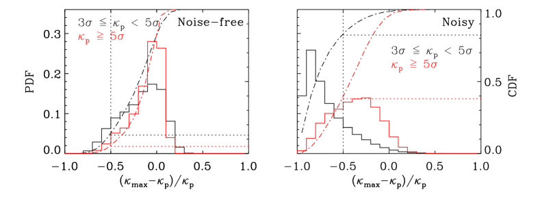
Figure 4: The distribution of the main lens plane contribution for different peak heights in noise-free (left) and noisy (right) fields. Here $\kappa_{\rm max}$ denotes the maximum contributor of the lens plane to a given convergence peak $\kappa_{\rm p}$. In addition, dot-dashed lines show the CDF of the fractional difference for the lensing peaks.

Table 1: The average fractional deviation, $\left<\left(\kappa_{\rm max}-\kappa_{\rm p}\right)/\kappa_{\rm p}\right>$, between the convergence of main lens plane and lensing peaks for sources at $z_{\rm s}=1.0$.

	noise-free	noisy
$3\sigma\leq\kappa_{\rm p}<5\sigma$	$-0.172\ (\pm\ 0.224)$	$-0.678\ (\pm\ 0.242)$
$\kappa_{\rm p}\geq 5\sigma$	$-0.110\ (\pm\ 0.170)$	$-0.378\ (\pm\ 0.254)$

Before we explore the correspondence between the lensing peaks and collapsed massive haloes along the LOS, we first examine the contribution from different lens planes for a given peak in the weak lensing maps. Fig. 4 shows the PDF of the main lens planes for lensing peaks with different heights in the noise-free (left panel) and noisy (right panel) convergence fields for sources at $z_{\rm s}=1.0$, where the main lens plane is the plane (with convergence $\kappa_{\rm max}$) which contributes mostly to a given lensing peak $\kappa_{\rm p}$. The black solid and red solid lines are for peaks with $0.054\ (3\sigma)\leq\kappa_{\rm p}<0.089\ (5\sigma)$ and $\kappa_{\rm p}\geq 0.089\ (5\sigma)$ respectively. Note that in the following, we will call the peaks in these two ranges as lower and high peaks unless otherwise specified. In table 1, we estimate the average fractional deviation between the main lens plane and convergence peak in weak lensing maps as $\left<\left(\kappa_{\rm max}-\kappa_{\rm p}\right)/\kappa_{\rm p}\right>$. In the noise-free fields, we find that lensing peaks can be dominated by only one lens plane, especially for peaks in $\kappa_{\rm p}\geq 5\sigma$, with an average fractional deviation of $-11\%$ as show in table 1. After adding the Gaussian shape noise, one noticeable feature seen from the right panel is that the PDF of fractional difference are significantly skewed. For high peaks in the range of $\kappa_{\rm p}\geq 5\sigma$, the deviation between $\kappa_{\rm max}$ and $\kappa_{\rm p}$ becomes larger, which implies that noise can boost peak heights in convergence maps (e.g., Fan, Shan, & Liu, 2010; Yang et al., 2011).

In Fig. 4 we also show the cumulative distribution functions (CDF) of the fractional difference using the dot-dashed lines. We define a peak to be single plane dominated peak (SPDP) if the main plane with $\kappa_{\rm max}$ larger than $50\%$ of the total peak height $\kappa_{\rm p}$. It is found that in the noise-free field $\sim 95\%$ of high peaks are SPDPs. While this fraction decreases to $\sim 87\%$ for the lower peaks. Adding random noise can bias the measurements of peak counts significantly as displayed in the right panel of Fig. 4. Only $\sim 18\%$ of lower peaks are SPDPs and about $62\%$ for high peaks. Note that in this part we do not distinguish the contribution from dark matter haloes or from the structure around haloes, such as filaments or sheet. In the next section, we will focus on the contribution from the dark matter haloes.

4.2 Correspondence between Convergence Peaks and Massive Haloes

Figure 5: A cartoon picture to illustrate how we search the matched dark matter haloes for a given lensing peakr. Following our ray-tracing simulation, light beam (blue line) can be gravitationally deflected at the position on the lens plane (red curves). In the picture the effect of lensing deflection is exaggerated. Black circles indicate the dark matter haloes reside in the light-cone. Red circles show the matched haloes if the traced light of the convergence peak crosses the virial radius of these haloes.

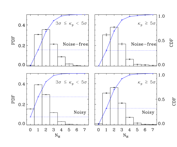
Figure 6: The number of dark matter haloes contributing to a given convergence peak in the noise-free fields (upper two panels) and noisy fields (lower two panels). Here we consider two samples with different peak heights, $3\sigma\leq\kappa_{\rm p}<5\sigma$ and $\kappa_{\rm p}\geq 5\sigma$, respectively. In addition, blue lines show the CDF of the number of the related haloes.

In general, convergence peaks are associated with collapsed haloes along the LOS, and it is also clear that this correspondence will be affected by the projection of LSS, noise, and also the observational effects, such as masking effects (e.g., White, van Waerbeke, & Mackey, 2002; Fan, Shan, & Liu, 2010; Liu et al., 2014; Shirasaki, Hamana, & Yoshida, 2015; Yuan et al., 2018). The height of convergence peak is closely related to the mass of the dark matter haloes along the LOS (e.g., Hamana, Takada, & Yoshida, 2004). In this section and Sec. 4.3, we focus on the contribution from massive haloes with $M_{\rm H}\geq 10^{13}{\rm M}_{\sun}$, which can produce a peak with a significance greater than $1\sigma$ in the convergence maps for sources at $z_{\rm s}=1.0$. In Sec. 4.4, we will focus on more massive haloes. Fig. 5 shows a cartoon picture to illustrate how we search the matched dark matter haloes for a given lensing peak. In the picture, red curves represent the configuration of spherical lens planes. Following our ray-tracing simulation, light beam (blue line) is gravitationally deflected at the position on the lens plane. Black and red circles indicate the dark matter haloes reside in the light-cone. For each lensing peak, we then find all matched dark matter haloes if the traced light of the convergence peak crosses the virial radii of these haloes (red circles).

In Fig. 6 we show the PDF of the number of haloes which are related to a given peak. Error bars are estimated by the Jackknife method. In the upper two panels, peaks are extracted from the noise-free convergence fields and lower panels show the results in the noisy convergence fields. For lensing peaks in the noise-free maps, we find that a large fraction ($>65\%$) of peaks can be related to more than one dark matter haloes along the line of sight. This result is consistent with previous work. In Yang et al. (2011), they examine the number of haloes required to account for $>50\%$ of the peak height, and found $\sim 55\%$ high peaks for sources at $z_{\rm s}=2$ with $\kappa\geq 0.11$ are contributed by more than one massive haloes on the line of sight. Moreover, as shown in the upper-left panel of Fig. 6, a few ($\lesssim 1\%$) of lower peaks have no matched massive haloes along the sightline. This can be explained by the projection of LSS or by the low mass haloes ($M_{\rm H}<10^{13}{\rm M}_{\sun}$) along the LOS in our simulation. Note that in this work we only focus on massive haloes ($\geq 10^{13}{\rm M}_{\sun}$) and we do not distinguish the contribution on convergence from low mass haloes ($<10^{13}{\rm M}_{\sun}$) with that from diffuse dark matter particles, or those from the LSS, such as filament or sheets. For simplicity, we use the LSS term to denote all these structures other than the massive haloes. After adding noise, more lensing peaks have no matched haloes on the line of sight in both peak height range. For high peaks, we find $\sim 2\%$ of lensing peaks without matched massive haloes. Compared with the upper-right panel, we conclude that these high peaks arise from the boosting effects of the noise field. While for lower peaks the PDF distributions imply that $\sim 15\%$ of false peaks is caused by the noise, and the fraction of peaks which relate to more than one dark matter haloes decrease to $\sim 45\%$.

Figure 7: The top panels show the probability distribution functions of the difference between halo contribution $\kappa_{\rm H}$ and lensing peak $\kappa_{\rm p}$ in the noise-free (left panel) and noisy (right panel) convergence maps. The fractional difference are calculated by $\left(\kappa_{\rm H}-\kappa_{\rm p}\right)/\kappa_{\rm p}$ for two different samples, $3\sigma\leq\kappa_{\rm p}<5\sigma$ and $\kappa_{\rm p}\geq 5\sigma$, respectively. The middle panels show the fractional difference between the lensing peak and the prediction of the only main halo along the line of sight, $\left(\kappa_{\rm mH}-\kappa_{\rm p}\right)/\kappa_{\rm p}$. The bottom panels show the fractional differences between $\kappa_{\rm mH}$ and $\kappa_{\rm H}$ for the given peaks. In addition, dot-dashed lines show the CDF of the fractional difference in each case.

Table 2: The average fractional deviation, $\left<\left(\kappa_{\rm H}-\kappa_{\rm p}\right)/\kappa_{\rm p}\right>$, between the halo prediction and lensing peak for sources at $z_{\rm s}=1.0$.

	noise-free	noisy
$3\sigma\leq\kappa_{\rm p}<5\sigma$	$-0.169\ (\pm\ 0.250)$	$-0.718\ (\pm\ 0.268)$
$\kappa_{\rm p}\geq 5\sigma$	$-0.128\ (\pm\ 0.176)$	$-0.394\ (\pm\ 0.271)$

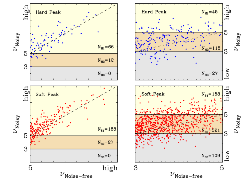
Figure 8: The distribution of the peak heights for the true peaks. Blue circles denote hard peaks and red circles are soft peaks. The numbers of peaks in different ranges of SNR are given by $N_{{\rm H}i}$ and $N_{{\rm S}i}$ respectively.

In order to study the contribution of massive haloes to a given lensing peak, we use Eq. 14 to predict the value of a peak height, $\kappa_{\rm H}$, by assuming that FOF haloes are described by the truncated NFW density profiles. In the top panels of Fig. 7, we show the difference between halo contribution $\kappa_{\rm H}$ and the total lensing peak $\kappa_{\rm p}$ in the noise-free (upper-left panel) and noisy (upper-right panel) convergence maps. It is seen that in case of no noise, the contribution is similar for high and lower peaks. In table 2 we give the average fractional deviation between halo predictions and convergence peaks, $\left<\left(\kappa_{\rm H}-\kappa_{\rm p}\right)/\kappa_{\rm p}\right>$. For high peaks in the noise-free field, an average fractional deviation of $-0.128$ is obtained, which means that LSS contributes 12.8 per cent to the lensing peaks with $\kappa_{\rm p}\geq 0.089$ for sources at $z_{\rm s}=1.0$. The contribution of LSS is increased to $16.9\%$ for lower peaks.

The right top panel show the case of noisy convergence field. Compared to the left top panel, it is seen that the distributions of both high and lower peaks are skewed to the left, with more skewness for lower peaks, indicating a significant fraction of peaks are false, and they are not related to any massive haloes. Table 2 shows that with noise the average fractional deviation is $-0.394$ for high peaks, and is $-0.718$ for lower peaks. The CDF distributions (dot-dashed lines) show that in the noise-free case, $96\%$ of high peaks are dominated by massive haloes which contribute more than half of the total peak height, and this fraction decreases to $88.4\%$ for lower peaks. In the case of noise, this fraction decreases to $60\%$ and $17\%$ for high and lower peaks.

Table 3: The average fractional deviation, $\left<\left(\kappa_{\rm mH}-\kappa_{\rm p}\right)/\kappa_{\rm p}\right>$, between the prediction of the main halo and lensing peak for sources at $z_{\rm s}=1.0$.

	noise-free	noisy
$3\sigma\leq\kappa_{\rm p}<5\sigma$	$-0.297\ (\pm\ 0.290)$	$-0.767\ (\pm\ 0.241)$
$\kappa_{\rm p}\geq 5\sigma$	$-0.219\ (\pm\ 0.215)$	$-0.472\ (\pm\ 0.281)$

Furthermore, we examine whether these lensing peaks are dominated by only one massive halo along the line of sight. In the middle panels of Fig. 7 we show the distribution of fractional difference between the convergence peaks and the main dark matter haloes, $\left(\kappa_{\rm mH}-\kappa_{\rm p}\right)/\kappa_{\rm p}$. Here the main dark matter halo is the halo contributing mostly to the given peak. The distributions are similar to those in the upper panels. Table 3 shows that the average fractional deviation in the noise-free field is to $21.9\%$ and $29.7\%$ for high and lower peaks respectively. With noise, the average fractional deviation is much worse. Similar as the definition of SPDP, we define a peak is a one halo dominated peak (OHDP) if $\kappa_{\rm mH}\geq 0.5\kappa_{\rm p}$. It is found that without noise, $84.7\%$ of high peaks are OHDPs and $69\%$ for lower peaks, indicating that without noise most high peaks are dominated by single massive halo, consistent with previous work (e.g., Hamana, Takada, & Yoshida, 2004; Yang et al., 2011). However, noise will significantly contaminate the peaks. For example only $\sim 48\%$ and $\sim 12\%$ of high and lower peaks are dominated by one single massive halo in case of noise. Moreover, the bottom panels show the fractional differences between $\kappa_{\rm mH}$ and $\kappa_{\rm H}$ for the given peaks. It is seen that the halo predictions are mostly contributed by the main haloes for both the noise-free and noisy cases. Here we note that these number are only for our selection of dark matter halo mass and our modeling of noise with its height and distribution.

Figure 9: The SNR distribution of convergences peak in the noisy field. Red circles denote all identified peaks in the noisy field, and blue circles are the matched true peaks. In the bottom panels, the PDFs show the number of peaks in the different range of SNR. $N_{{\rm t}i}$ denotes the total number of peaks in the noisy field, and $N_{{\rm p}i}$ is the number of matched peaks from the noise-free field.

4.3 Effects of Noise on the Convergence Peak and Halo Connection

Table 4: Counts of peaks in our convergence field. The numbers in parentheses in the middle and right columns show the number of peaks per 1 ${\rm deg}^{2}$ in our mocked sky.

	Case	Number
		high peaks	lower peaks
I	peak in noise-free field	407 (0.21)	2095 (1.07)
II	peak in noisy field	821 (0.42)	11267 (5.75)
III	peak in the pure noise field	2 (0.001)	3898 (1.99)

The above peak statistics analyses show that convergence peaks can be significantly affected by galaxy shape noise. In Fan, Shan, & Liu (2010), they developed a theoretical model to predict the numbers of convergence peaks taking into account the effects of noise in the weak lensing maps. They concluded that the noise not only produces pure noise peaks in the convergence field, but also affects the heights of true peaks. In addition, the pure noise peaks will be enhanced in halo regions (the virial radius). In this work we further study the effects of noise on the correspondence between the peaks and massive haloes. Table 4 shows the peak counts in our convergence field for the high and lower peaks. It is found that without noise, the number density of high and lower peaks is 0.21 ${\rm deg}^{-2}$ and 1.07 ${\rm deg}^{-2}$ respectively. Noise will double the number of high peak to 0.42 ${\rm deg}^{-2}$, and raise the number of lower peaks to 5.75 ${\rm deg}^{-2}$. The number density of peaks in the noisy field is consistent with that of Giocoli et al. (2018).

In order to examine the effect of noise on the true peaks, we then check how many true peaks survived and how much of their SNR change. Here we distinguished two cases. For a peak in the noise-free convergence field, if it is still a peak in the noisy field, we call it as a hard peak. If the true peak disappear in the noisy field, but its neighbor (the angular distance is less than one $\rm arcmin$, more than twice of the resolution of our simulation with 0.43 $\rm arcmin$) appears as a peak, we call the peak in the noise-free field as a soft peak. We call these two kinds of peak as true peak and the others noise-free peaks are defined as destroyed peaks. Note that true peaks are defined as the local maxima in the noise-free convergence field. Thus a fraction of true peaks are caused by projection effects. This projection effects of LSS have been shown in Fig. 6 and Fig. 7.

Fig. 8 shows the comparison of SNR of the peak pairs. The upper panels are for hard peaks and lower for soft peaks. The numbers of hard/soft peaks in different ranges of SNR are given by $N_{{\rm H}i}$ and $N_{{\rm S}i}$ respectively. In the $\sim 2000\ {\rm deg}^{2}$ of our mock sky, we find a total number of 407 and 2095 for the high and lower peaks in the noise-free field (see table 4 for those numbers). For those high peaks, it is found that the total number of survived peaks is $N_{\rm H1}+N_{\rm H2}+N_{\rm H3}+N_{\rm S1}+N_{\rm S2}+N_{\rm S3}=293$, about $72\%$ of the original high peaks. The remaining $114$ peaks, $28\%$ of the total, are destroyed by noise. Among those survived peaks, $78\ (27\%)$ peaks are hard peaks and others are soft peaks. Among those hard high peaks, about $85\%$ are still high peaks, but others are downgraded to low peaks. In the right panel we show the case of the low peaks. It is seen that only $47\%$ ($975$ of $2095$) peaks survive the adding of noise. More than half of original peak are destroyed.

Previously we search the noise-free field and find their correspondences in the noisy field. Now we start from the noisy field and find their correspondences in the noise-free field. Fig. 9 shows the SNR distribution of peaks identified in the noisy field, and the PDF in the bottom panels show the number of peaks in the given ranges of SNR, where $N_{{\rm t}i}$ denotes the total number of convergence peak in the noisy field and $N_{{\rm p}i}$ is the number of matched peaks (with $N_{\rm p1}$/$N_{\rm p2}$ denoting the original high/lower peaks) from the noise-free field. Thus the matched peaks here contain both hard peaks and soft peaks in Fig. 8, which means $N_{\rm p1}=N_{\rm H1}+N_{\rm S1}$ for high peaks and $N_{\rm p2}=N_{\rm H2}+N_{\rm S2}$ for lower peaks. For the $821$ high peaks in the noisy field, $493\ (60\%)$ of them are true peaks in the noise-free field, and among which $254$ (around $254/493\sim 51\%$) are original high peaks. The remaining $40\%$ are not peaks in the noise-free field, but are boosted as peaks by noise. In the right panel, it is found that there is $11267$ lower peaks in the noisy field, but only $20\%\ (2428/11267)$ are true peaks in the noise-free convergence field. These results suggest that for high peaks in the noisy field there are significant fraction of them are true peaks in the density map, and around $30\%$ are true high peaks.

4.4 Mass Dependence of the Correspondence between Peaks and Haloes

Figure 10: Similar as Fig. 6, but only with halo mass $M_{\rm H}\geq 10^{14}{\rm M}_{\sun}$.

As noted in Sec. 4.1 we only consider haloes with mass larger than $10^{13}{\rm M}_{\sun}$ and Fig. 7 shows that most of high peaks are dominated by a main halo along the LOS (OHDPs). In this section, we only take account of dark matter haloes with $M_{\rm H}\geq 10^{14}{\rm M}_{\sun}$ to examine the correspondence between convergence peaks and dark matter haloes.

Similar as Fig. 6 and Fig. 7, the results are given in Fig. 10 and Fig. 11. As shown in Fig. 10, we display the related halo numbers in the noise-free (upper) and noisy field (lower). Comparing the upper-right panels of Fig. 6 and Fig. 10, we conclude most of high peaks in noise-free field can be related with only one massive halo larger than $10^{14}{\rm M}_{\sun}$, and about $\sim 20\%$ of them are associated with more than one massive haloes larger than $10^{14}{\rm M}_{\sun}$ along the LOS. For the lower peaks in the upper-left panel of Fig. 10, we find that $18\%$ of peaks do not have matched haloes with mass larger than $10^{14}{\rm M}_{\sun}$. Compared with Fig. 6, these not matched peaks are attributed to one or more haloes with mass in $10^{13}{\rm M}_{\sun}\leq M_{\rm H}<10^{14}{\rm M}_{\sun}$. After adding noise, about $70\%$ high peaks can relate to only one massive halo (lower-right), but $70\%$ of lower peaks do not have matched massive haloes (lower-left), which can be related with less massive dark matter haloes or caused by the noise ($\sim 15\%$). By comparing with the results of Fig. 6, we find that massive haloes with $M_{\rm H}\geq 10^{14}{\rm M}_{\sun}$ can be effectively detected by high peaks with $\kappa_{\rm p}\geq 5\sigma$, but only about $30\%$ lower peaks are related with such massive haloes.

Furthermore, Fig. 11 shows the fractional difference between convergence peaks and the main halo as in Fig. 7. In the noise-free field (left panel), the average fractional deviation is $-0.218$ for the high peaks, which is almost same as that in table 3. This consistency means that high peaks are dominated by massive haloes with $M_{\rm H}\geq 10^{14}{\rm M}_{\sun}$. For lower peaks, the deviation increase to $-0.376$, which is slightly larger than that in table 3. This is reasonable as that we find $\sim 18\%$ of lower peaks do not have matched haloes with $M_{\rm H}\geq 10^{14}{\rm M}_{\sun}$ in Fig. 10. These peaks should be explained by the contribution of lower mass haloes in $10^{13}{\rm M}_{\sun}\leq M_{\rm H}<10^{14}{\rm M}_{\sun}$.

The distribution of CDF in Fig. 11 shows almost same results as in Fig. 7, which means dark matter haloes with $M_{\rm H}\geq 10^{14}{\rm M}_{\sun}$ should be the main contributor to the convergence peaks although lower mass haloes are also important to give $\sim 5\%$ difference for lower peaks. After adding noise, we find about 50% high peaks can be dominated by the massive haloes with $M_{\rm H}\geq 10^{14}{\rm M}_{\sun}$, but only 10% lower peaks are dominated by one massive halo along the LOS. This effective mass detection in weak lensing convergence peaks is also found in the literature (e.g., Hamana, Takada, & Yoshida, 2004; Shan et al., 2018).

Figure 11: Similar as Fig. 7, but only with halo mass $M_{\rm H}\geq 10^{14}{\rm M}_{\sun}$.

5 CONCLUSION AND DISCUSSION

In this paper, we focus on lensing peaks to examine the correspondence between weak lensing convergence peaks and dark matter haloes. Following the multiple lens plane algorithm on the curved sky, We performed a high-spatial and high-mass resolution ray-tracing simulation. Based on these simulated convergence maps, we examine the abundance of lensing peaks and the correspondence between peaks and massive haloes along the LOS. For each lensing peak, we try to search the corresponding dark matter haloes, if the selected peak locates in the virial radius of these haloes. Two thresholds, $\kappa=3\sigma(0.054)$ and $5\sigma(0.089)$, are used in our analysis and the results are summarized as follows.

• In the noise-free field, we find that more than $65\%$ peaks are related to more than one massive haloes with mass in $M_{\rm H}\geq 10^{13}{\rm M}_{\sun}$. A few ($\lesssim 1\%$) of lower peaks in $3\sigma\leq\kappa_{\rm p}<5\sigma$ arise without matched massive haloes along the LOS. This should be contributed by the projection effect of LSS. By assuming these matched haloes with the truncated NFW profile, we then test the correspondence of peak heights between weak lensing maps and the related massive haloes. The fractional difference between halo predictions and lensing peaks, $(\kappa_{\rm H}-\kappa_{\rm p})/\kappa_{\rm p}$, shows that LSS contributes $12.8\%$ to the lensing peaks with $\kappa_{\rm p}\geq 0.089$ for sources at $z_{\rm s}=1.0$. The contribution from LSS increase to $16.9\%$ for lower peaks. On other hand, as shown by the cumulative distribution functions, about $96\%$ peaks is dominated by the massive dark matter haloes along the LOS for high peaks, and for lower peaks the fraction is about $88.4\%$. Moreover, we further examine the correspondence between the lensing peaks and the main dark matter haloes. The result shows that $84.7\%$ high peaks can be dominated by one single halo and only $69\%$ for the lower convergence peaks.

• In the noisy field, convergence maps are significantly modulated by the noise and the asymmetric double peaks arise due to the noise modulation. After adding noise, a number of false peaks arise, especially at the lower SNR. About $60\%$ high peaks are true peaks, but only $20\%$ for the lower peaks. The average fractional deviation show that for high peaks the difference between convergence peaks and the predictions from total matched haloes is $39.4\%$ and $60\%$ of them are halo dominated, but for lower peaks only $17\%$ are halo dominated. If we only consider the main dark matter halo with the maximum contribution in the halo prediction, we find the average fractional deviation slightly increase to $47.2\%$ and the fraction of peaks dominated by the main halo decrease to $48\%$.

Furthermore, considering that most of high peaks are OHDPs, we take account of more massive haloes with $M_{\rm H}\geq 10^{14}{\rm M}_{\sun}$ to examine the correspondence between convergence peaks and dark matter haloes. We find dark matter haloes with $M_{\rm H}\geq 10^{14}{\rm M}_{\sun}$ are the main contributor to the convergence peaks although lower mass haloes are also important to give $\sim 5\%$ difference for lower peaks. After adding noise, we find about $50\%$ high peaks are dominated by the massive haloes with $M_{\rm H}\geq 10^{14}{\rm M}_{\sun}$, but only $10\%$ lower peaks are dominated by one massive halo along the LOS. Our results show that massive haloes, especially with $M_{\rm H}\geq 10^{14}{\rm M}_{\sun}$, can be effectively detected by the high weak lensing convergence peaks. In the lower peaks with $3\sigma\leq\kappa<5\sigma$, the peak heights are significantly modified by the noise effect. When we use it to probe cosmology and constrain the model of structure formation, we should carefully address the effects of galaxy shape noise, LSS projection and also the observational effects, especially for low peaks.

References

- Amendola, Kunz, & Sapone (2008) Amendola L., Kunz M., Sapone D., 2008, JCAP, 4, 013
- Bartelmann & Schneider (2001) Bartelmann M., Schneider P., 2001, PhR, 340, 291
- Bartelmann & Maturi (2017) Bartelmann M., Maturi M., 2017, SchpJ, 12, 32440
- Becker (2013) Becker M. R., 2013, MNRAS, 435, 115
- Calabretta & Roukema (2007) Calabretta M. R., Roukema B. F., 2007, MNRAS, 381, 865
- Cardone et al. (2013) Cardone V. F., Camera S., Mainini R., Romano A., Diaferio A., Maoli R., Scaramella R., 2013, MNRAS, 430, 2896
- Dark Energy Survey Collaboration et al. (2016) Dark Energy Survey Collaboration, et al., 2016, MNRAS, 460, 1270
- Das & Bode (2008) Das S., Bode P., 2008, ApJ, 682, 1-13
- de Jong et al. (2015) de Jong J. T. A., et al., 2015, A&A, 582, A62
- Dietrich & Hartlap (2010) Dietrich J. P., Hartlap J., 2010, MNRAS, 402, 1049
- Duffy et al. (2008) Duffy A. R., Schaye J., Kay S. T., Dalla Vecchia C., 2008, MNRAS, 390, L64
- Fan, Shan, & Liu (2010) Fan Z., Shan H., Liu J., 2010, ApJ, 719, 1408
- Foreman, Becker, & Wechsler (2016) Foreman S., Becker M. R., Wechsler R. H., 2016, MNRAS, 463, 3326
- Fosalba et al. (2015) Fosalba P., Gaztañaga E., Castander F. J., Crocce M., 2015, MNRAS, 447, 1319
- Fosalba et al. (2008) Fosalba P., Gaztañaga E., Castander F. J., Manera M., 2008, MNRAS, 391, 435
- Fu et al. (2008) Fu L., et al., 2008, A&A, 479, 9
- Górski et al. (2005) Górski K. M., Hivon E., Banday A. J., Wandelt B. D., Hansen F. K., Reinecke M., Bartelmann M., 2005, ApJ, 622, 759
- Giocoli et al. (2018) Giocoli C., Moscardini L., Baldi M., Meneghetti M., Metcalf R. B., 2018, arXiv, arXiv:1801.01886
- Hamana et al. (2012) Hamana T., Oguri M., Shirasaki M., Sato M., 2012, MNRAS, 425, 2287
- Hamana, Takada, & Yoshida (2004) Hamana T., Takada M., Yoshida N., 2004, MNRAS, 350, 893
- Heymans et al. (2013) Heymans C., et al., 2013, MNRAS, 432, 2433
- Hildebrandt et al. (2017) Hildebrandt H., et al., 2017, MNRAS, 465, 1454
- Hinshaw et al. (2013) Hinshaw G., et al., 2013, ApJS, 208, 19
- Jain & Van Waerbeke (2000) Jain B., Van Waerbeke L., 2000, ApJ, 530, L1
- Jee et al. (2016) Jee M. J., Tyson J. A., Hilbert S., Schneider M. D., Schmidt S., Wittman D., 2016, ApJ, 824, 77
- Kilbinger (2015) Kilbinger M., 2015, RPPh, 78, 086901
- Kilbinger (2003) Kilbinger M., 2003, astro, arXiv:astro-ph/0309482
- Kilbinger et al. (2017) Kilbinger M., et al., 2017, MNRAS, 472, 2126
- Kratochvil, Haiman, & May (2010) Kratochvil J. M., Haiman Z., May M., 2010, PhRvD, 81, 043519
- Laureijs et al. (2011) Laureijs R., et al., 2011, arXiv, arXiv:1110.3193
- Lemos, Challinor, & Efstathiou (2017) Lemos P., Challinor A., Efstathiou G., 2017, JCAP, 5, 014
- Li et al. (2005) Li G.-L., Mao S., Jing Y. P., Bartelmann M., Kang X., Meneghetti M., 2005, ApJ, 635, 795
- Li et al. (2016) Li S.-J., et al., 2016, RAA, 16, 130
- Lin & Kilbinger (2015) Lin C.-A., Kilbinger M., 2015, A&A, 576, A24
- Liu & Haiman (2016) Liu J., Haiman Z., 2016, PhRvD, 94, 043533
- Liu et al. (2016) Liu X., et al., 2016, PhRvL, 117, 051101
- Liu et al. (2015) Liu X., et al., 2015, MNRAS, 450, 2888
- Liu et al. (2014) Liu X., Wang Q., Pan C., Fan Z., 2014, ApJ, 784, 31
- Lombardi & Bertin (1999) Lombardi M., Bertin G., 1999, A&A, 348, 38
- LSST Science Collaboration et al. (2009) LSST Science Collaboration, et al., 2009, arXiv, arXiv:0912.0201
- Marian et al. (2013) Marian L., Smith R. E., Hilbert S., Schneider P., 2013, MNRAS, 432, 1338
- Martinet et al. (2018) Martinet N., et al., 2018, MNRAS, 474, 712
- Maturi et al. (2010) Maturi M., Angrick C., Pace F., Bartelmann M., 2010, A&A, 519, A23
- Maturi, Fedeli, & Moscardini (2011) Maturi M., Fedeli C., Moscardini L., 2011, MNRAS, 416, 2527
- Maturi et al. (2005) Maturi M., Meneghetti M., Bartelmann M., Dolag K., Moscardini L., 2005, A&A, 442, 851
- Mellier (1999) Mellier Y., 1999, ARA&A, 37, 127
- Meylan et al. (2006) Meylan G., Jetzer P., North P., Schneider P., Kochanek C. S., Wambsganss J., 2006, Saas-Fee Advanced Course 33: Gravitational Lensing: Strong, Weak and Micro (Berlin: Springer)
- Miyazaki et al. (2007) Miyazaki S., Hamana T., Ellis R. S., Kashikawa N., Massey R. J., Taylor J., Refregier A., 2007, ApJ, 669, 714
- Miyazaki et al. (2015) Miyazaki S., et al., 2015, ApJ, 807, 22
- Navarro, Frenk, & White (1997) Navarro J. F., Frenk C. S., White S. D. M., 1997, ApJ, 490, 493
- Navarro, Frenk, & White (1996) Navarro J. F., Frenk C. S., White S. D. M., 1996, ApJ, 462, 563
- Schneider et al. (2017) Schneider M. D., Ng K. Y., Dawson W. A., Marshall P. J., Meyers J. E., Bard D. J., 2017, ApJ, 839, 25
- Schneider, Ehlers, & Falco (1992) Schneider P., Ehlers J., Falco E. E., 1992, grle.book, 112
- Shan et al. (2014) Shan H. Y., et al., 2014, MNRAS, 442, 2534
- Shan et al. (2012) Shan H., et al., 2012, ApJ, 748, 56
- Shan et al. (2018) Shan H., et al., 2018, MNRAS, 474, 1116
- Shirasaki (2017) Shirasaki M., 2017, MNRAS, 465, 1974
- Shirasaki, Hamana, & Yoshida (2015) Shirasaki M., Hamana T., Yoshida N., 2015, MNRAS, 453, 3043
- Springel (2010) Springel V., 2010, ARA&A, 48, 391
- Springel (2005) Springel V., 2005, MNRAS, 364, 1105
- Takada & Jain (2003) Takada M., Jain B., 2003, MNRAS, 340, 580
- Teyssier et al. (2009) Teyssier R., et al., 2009, A&A, 497, 335
- Tweed et al. (2017) Tweed D., Yang X., Wang H., Cui W., Zhang Y., Li S., Jing Y. P., Mo H. J., 2017, ApJ, 841, 55
- Van Waerbeke et al. (2001) Van Waerbeke L., et al., 2001, A&A, 374, 757
- van Waerbeke (2000) van Waerbeke L., 2000, MNRAS, 313, 524
- Wang et al. (2014) Wang H., Mo H. J., Yang X., Jing Y. P., Lin W. P., 2014, ApJ, 794, 94
- Wang et al. (2016) Wang H., et al., 2016, ApJ, 831, 164
- Wei et al. (2018) Wei C., et al., 2018, ApJ, 853, 25
- White, van Waerbeke, & Mackey (2002) White M., van Waerbeke L., Mackey J., 2002, ApJ, 575, 640
- Yang et al. (2011) Yang X., Kratochvil J. M., Wang S., Lim E. A., Haiman Z., May M., 2011, PhRvD, 84, 043529
- Yuan et al. (2018) Yuan S., Liu X., Pan C., Wang Q., Fan Z., 2018, ApJ, 857, 112
- Zorrilla Matilla et al. (2016) Zorrilla Matilla J. M., Haiman Z., Hsu D., Gupta A., Petri A., 2016, PhRvD, 94, 083506