ChromaStarAtlas: Browser-based visualization of the ATLAS9 stellar structure and spectrum grid

Abstract

ChromaStaraAtlas (CSA) is a web application that uses the ChromaStar (CS) user interface (UI) to allow users to navigate and display a subset of the uniformly computed comprehensive ATLAS9 grid of atmosphere and spectrum models. It provides almost the same functionality as the CS UI in its more basic display modes, but presents the user with primary and post-processed outputs, including photometric color indices, based on a properly line blanketed spectral energy distribution (SED). CSA interpolates in logarithmic quantities within the subset of the ATLAS9 grid ranging in $T_{\rm eff}$ from 3500 to 25000 K, in $\log g$ from 0.0 to 5.0, and in $[{{\rm Fe}\over{\rm H}}]$ from 0.0 to -1.0 at a fixed microturbulence parameter of 2 km s^-1, and presents outputs derived from the monochromatic specific intensity distribution, $I_{\lambda}$, in the $\lambda$ range from 250 to 2500 nm, and performs an approximate continuum rectification of the corresponding flux spectrum $F_{\lambda}$ based on its own internal model of the corresponding continuous extinction distribution, $\kappa^{\rm C}_{\lambda}$, based on the procedures of CS. Optional advanced plots can be turned on that display both the primary atmospheric structure quantities from the public ATLAS9 data files, and secondary structure quantities computed from internal modeling. Unlike CS, CSA allows for activities in which students derive $T_{\rm eff}$ values from fitting observed colors. The application may be found at www.ap.smu.ca/$\sim$ishort/OpenStars.

I Introduction

Short 2014 described ChromaStar (CS), a general approximate atmospheric structure and emergent radiation field modeling and post-processing code written in JavaScript (JS), the language of Web browsers, in which the visualization component was written in HTML. This provides access to parameter perturbation experiments in stellar and some exoplanet astrophysics for pedagogical purposes in way that is robustly platform-independent and suitable for commonplace personal and portable devices. Because the modeling is executed on the client side, both the full source code and the underlying atmospheric and radiation field structures that have been computed are in the browser memory. As a result, a more advanced user can optionally display the modeled structures, and interact with the source code through the browser’s developer tools while they are running it. A limitation of the client-side JS modeling is that CS is limited to a line list of about twenty atomic lines and two TiO bands treated in the just-overlapping-line (JOLA) approximation. Another limitation is that CS achieves its execution speed by simply re-scaling the $T_{\rm kin}(\log\tau)$ structure with $T_{\rm eff}$ to obviate the need for converging thermal equilibrium, so the accuracy of the $T_{\rm kin}(\log\tau)$ structure is limited and this in turn affects the accuracy of computed spectral features. Short 2016 described ChromaStarServer (CSServ) a significant variation in which the CS user interface (UI) is used to interact with and visualize the results of a server-side modeling code written in Java based on the same modeling methods as CS, but with a much larger line list ($\sim$ 26  000 lines as of this writing). However, CSServ only draws from this line list to compute the high resolution spectrum in a limited $\lambda$ range specified by the user, and, as with CS, the overall spectral energy distribution (SED) is un-blanketed. As a result, the photometric color indices computed with either CSServ or CS are not comparable to observed colors.

Here we present ChromaStarAtlas (CSA), a browser-based application for rendering and visualizing the uniformly computed, comprehensive grid of line-blanketed thermal equilibrium stellar atmospheric and surface intensity models computed with the ATLAS9 general stellar atmospheric modeling code (Castelli & Kurucz 2006, Castelli & Kurucz 2004, Kurucz 2014). Like CSServ, the atmospheric- and spectrum-related distributions are prepared on the server side in Java, and the results sent to the client UI for some post-processing and visualization. As of this writing, CSA accommodates a subset of the full ATLAS9 grid consisting of models in the effective temperature ($T_{\rm eff}$) range of 3500 to 25000 K, the surface gravity ($\log g$) range of 0.0 to 5.0, with scaled solar abundance in the metallicity ($[{\rm Fe}/{\rm H}]$) range 0.0 to -1.0 with a microturbulent velocity parameter ($\xi_{\rm T}$) of 2.0 km s^-1, and this is a large enough region of parameter space to be useful for many important pedagogical demonstrations and labs. In Section II we discuss the methods used to quickly read the ATLAS9 grid and to interpolate within it, and in Section III we discuss some of the key activities CSA allows for, with emphasis on the contrast with CS and CSServ. The application may be found at www.ap.smu.ca/$\sim$ishort/OpenStars.

II Methods

II.1 ATLAS9 grid preparation

Details of the ATLAS9 model grid can be found in Castelli & Kurucz 2006 and Castelli & Kurucz 2004 and here we review those grid properties that are especially relevant to the challenge of quickly reading and processing the data files. The ATLAS9 model grids span a range in $T_{\rm eff}$ from 3500 to 50000 K with a sampling, $\Delta T_{\rm eff}$, of 250 K for $T_{\rm eff}<13000$ K and of 1000 K for $T_{\rm eff}\geq 13000$ K, and span a range in $\log g$ from as low as 0.0 at the cool end of the grid to 5.0 for all $T_{\rm eff}$ values, with a sampling, $\Delta\log g$ of 0.5, for a total of 476 $(T_{\rm eff},\log g)$ combinations.

For scaled solar models of a given combination of $[{\rm Fe}/{\rm H}]$ and $\xi_{\rm T}$, atmospheric structures for all 476 $(T_{\rm eff},\log g)$ combinations computed with the “new” opacity distribution functions (OFDs) are in one ascii character-data file following the naming convention of the form of ap00k2odfnew.dat (for the case of models of $[{\rm Fe}/{\rm H}]=0.0$ and $\xi_{\rm T}=2.0$ km s^-1), and have a size of $\sim 4.5$ Mbytes. Each structure block includes the values of the column mass density $\bar{\rho}$ (“RHOX”) in g cms^-2 tabulated at 72 depth points, and this serves as the independent depth variable. Additional columns are 1) Kinetic temperature $T_{\rm kin}$ (“T”) in K, 2) Total gas pressure $P_{\rm gas}$ (“P”) in dynes cms^-2, 3) Free electron number density $n_{\rm e}$ (“XNE”) in cms^-3, 4) Rosseland mean mass extinction $\kappa_{\rm Ros}$ (“ABROSS”) in cm² g^-1, 5) Radiative acceleration (“ACCRAD”) in cm s^-2, 6) Turbulent velocity (“VTURB”) in cm s^-1, 7) Convective flux $F_{\rm conv}$ (“FLXCNV”), 8) Velocity of convective cells (“CONV”) in cm s^-1, and 9) Local sound speed (“VELSND”) cm s^-1. The corresponding surface specific intensity distributions, $I_{\nu}(\lambda,\cos\theta,\tau=0)$, for all 476 $(T_{\rm eff},\log g)$ combinations for a given $([{\rm Fe}/{\rm H}],\xi_{\rm T})$ combination are in ascii character-data files following the naming convention of the form of ip00k2.pck19 (for the case of models of $[{\rm Fe}/{\rm H}]=0.0$ and $\xi_{\rm T}=2.0$ km s^-1) and have a size of over 67 Mbytes. The $I_{\nu}$ distribution is tabulated at 1221 $\lambda$ values ranging from 9.09 to 16000 nm at 17 $\cos\theta$ values ranging from 1.0 (disk center) to 0.01 for a total of 20  757 $I_{\nu}$ values per model (we note that the $\Delta\cos\theta$ sampling is non-uniform, decreasing with decreasing $\cos\theta$, but is not the usual Gauss-Legendre quadrature). The $I_{\nu}$ value at disk center, $I_{\nu}(\cos\theta=1)$, is given in erg s^-1 cm^-2 ster^-1 Hz^-1, and as the value of $10^{5}\times I_{\nu}/I_{\nu}(\cos\theta=1)$ for the subsequent 16 $\cos\theta$ points.

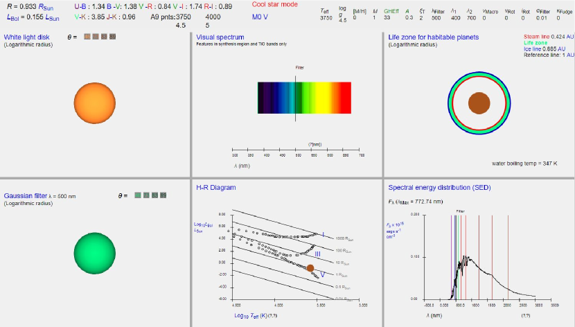
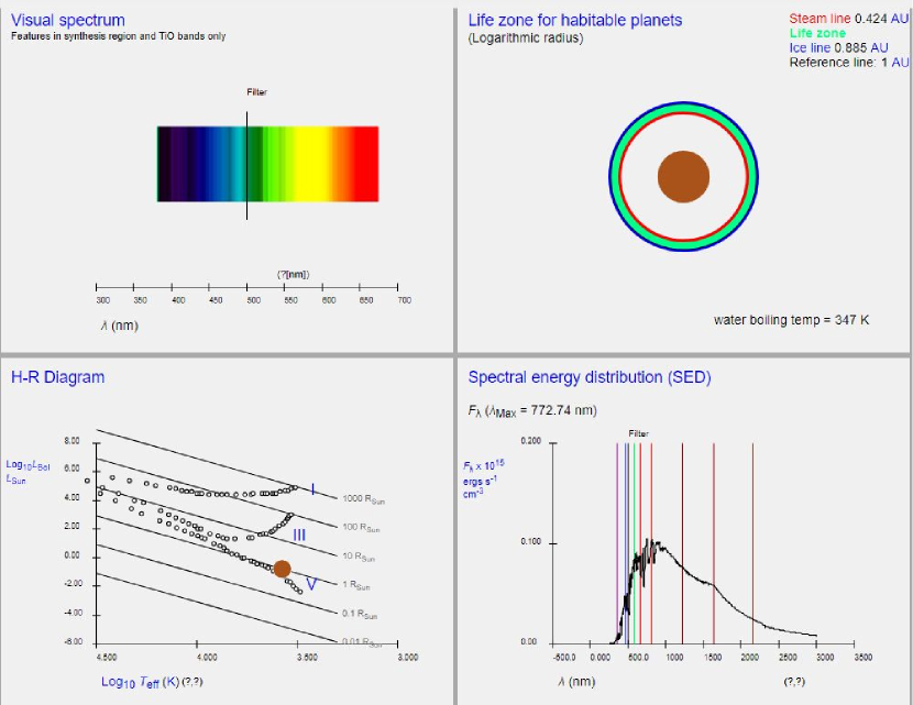
For the subset of all models of $T_{\rm eff}\leq 25000$ K (406 models), we have converted the ascii structure data files for the grids of scaled-solar $[{\rm Fe}/{\rm H}]$ value equal to 0.0, -0.5, and -1.0 and $\xi_{\rm T}$ value of 2 km s^-1 computed with the “new” ODFs (“ap00k2odfnew.dat”, “am05k2odfnew.dat”, and “am10k2odfnew.dat”) into byte data for rapid reading by CSA. This is performed with the auxiliary Java procedure AtlasModelServer. The byte-data files contain the 1) $\bar{\rho}$, 2) $T_{\rm kin}$, 3) $P_{\rm gas}$, 4) $n_{\rm e}$, 5) $\kappa_{\rm Ros}$, and 6) $F_{\rm conv}$ structures. The first five of these are primary atmospheric modeling quantities that are necessary to compute other quantities of general interest, and the fifth is useful for indicating in the visual output the depth where the atmospheric convective zone begins. The byte-data file also contains the metallicity parameter $[{\rm Fe}/{\rm H}]$ and the logarithmic abundances, $\log N(Z)/N_{\rm H}$, for 100 elements from He ($Z=2$) to Es ($Z=99$), as specified in the ATLAS9 structure file, although many of these for Po ($Z=84$) and higher appear to be upper limits ($\log N(Z)/N_{\rm H}=-20.0$). We have also pre-processed and converted the corresponding ascii $I_{\nu}$ distributions (files “ip00k2.pck19”, “im05k2.pck”, and “im10k2.pck”) for all models of $T_{\rm eff}\leq 25000$ K to byte data with the auxiliary Java procedure AtlasSpecServer. The pre-processing includes conversion of the $10^{5}\times I_{\nu}/I_{\nu}(\cos\theta=1)$ values to absolute $I_{\nu}$ values for all $\cos\theta$ points, conversion of the $I_{\nu}$ distribution to the $I_{\lambda}$ distribution observable with diffraction grating spectrographs, and, for all atmospheric and spectrum quantities, “numeric compression” by conversion to logarithmic units. To manage the execution time and memory requirements of CSA, we only include every second depth point in the structure, for a total of 36 depths, and $I_{\lambda}$ values at a subset of the $\lambda$ values ranging from 250.50 to 2505.00 nm (608 $\lambda$ values) and at every second $\cos\theta$ point (nine $\cos\theta$ values, including $\cos\theta=1$ and $0.01$), for a total of 5472 $\log I_{\lambda}$ values per model. Figs. 1 and 2 show a variety of renderings and signals of a model star of ($T_{\rm eff}/\log g/[{\rm Fe}/{\rm H}]$) equal to (3750 K/4.5/0.0) that show the importance of line blanketing.

II.2 CSA processing

For a given set of stellar parameters input by the user, ($T_{\rm eff}$, $\log g$, and $[{\rm Fe}/{\rm H}]$), CSA finds the two bracketing models in each of the $T_{\rm eff}$ and $\log g$ dimensions (four brackets altogether) and interpolates the $\log\bar{\rho}$, $\log T_{\rm kin}$, $\log P_{\rm gas}$, $\log n_{\rm e}$, $\log\kappa_{\rm Ros}$, $\log F_{\rm conv}$, and $\log I_{\lambda}(\lambda,\cos\theta)$ values in each of the grids of $[{\rm Fe}/{\rm H}]$ equal to 0.0 and -1.0. A linear interpolation is first performed in $\log T_{\rm eff}$ at each of the two bracketing $\log g$ values, then in $\log g$, then in $[{\rm Fe}/{\rm H}]$. It then constructs the surface flux distribution $F_{\lambda}(\tau=0)$ from the interpolated $I_{\lambda}$ distribution using the $2D$ disk integration method of CSServ (see (Short 2016)). If a user specifies a ($T_{\rm eff}$, $\log g$, and $[{\rm Fe}/{\rm H}]$) combination that falls outside the subset of the ATLAS9 grid currently accommodated (eg. a low $\log g$ value at high $T_{\rm eff}$ value), then the nearest grid model is taken.

CSA constructs the $\log\tau_{\rm Ros}$ scale from the interpolated $\log\bar{\rho}$ and $\log\kappa_{\rm Ros}$ distributions, and the partial $e^{-}$ pressure structure $\log P_{\rm e}(\tau)$ from the interpolated $\log T_{\rm kin}$ and $\log n_{\rm e}$ structures. It then computes the total number density of gas particles $N_{\rm gas}(\tau)$, mass density $\rho(\tau)$, and mean molecular weight $\mu(\tau)$ structures from the ATLAS9 abundance distribution $\log N(Z)/N_{\rm H}$ scaled by the input $[{\rm Fe}/{\rm H}]$ value. It then computes the total continuous opacity $\kappa^{\rm C}_{\lambda}(\tau)$ resulting from bound-free (b-f), free-free (f-f) and Rayleigh scattering from various species involving H and He, Thomson scattering from free electrons, and ground-state b-f opacity from seven metals (C I, Mg I, Mg II, Al I, Si I, Si II, and Fe I) that are important in the UV band, and computes its own independent continuum optical depth scale $\log\tau^{\rm C}(\log\tau_{\rm Ros})$. It then evaluates the formal solution of the hydrostatic equilibrium (HSE) equation on its internal $\log\tau^{\rm C}$ scale, and computes the geometric depth scale $z(\log\tau^{\rm C})$. CSA then evaluates the formal solution of the radiative transfer equation (RTE) using its internal $\kappa^{\rm C}_{\lambda}$ distribution and $\log\tau^{\rm C}$ scale to compute the continuum surface intensity, $I^{\rm C}_{\lambda}(\cos\theta,\tau=0)$, and flux $F^{\rm C}_{\lambda}(\tau=0)$ distributions, and it uses the latter to approximately continuum normalize (rectify) the line-blanketed $F_{\lambda}(\tau=0)$ spectrum. The procedure results in an $F_{\lambda}(\tau=0)/F^{\rm C}_{\lambda}(\tau=0)$ spectrum that is generally continuum normalized for late-type stars to within a factor of a few around 400 nm and more accurately around 700 nm. The procedures for computing these secondary quantities are those as presented in Gray 2005 and are taken from CSServ (Short 2016.

Line labels

Although CSA is not performing spectrum synthesis of its own, we nevertheless read the line list as described for CSServ (Short 2016) so that we can provide line identification labels in the output within the $\lambda$ range 260 to 2600 nm. The line list is drawn from the NIST Atomic Spectra Database (Kramida et al. 2015) and contains only a modest subset of the lines in the ATLAS9 line list and is not necessarily consistent with the line list used to compute the spectrum, but we expect that for the relatively well-known lines that are in the NIST database the labels will generally be relevant.

Limb darkening coefficients

We use the internal $I^{\rm C}_{\lambda}(\cos\theta)/I^{\rm C}_{\lambda}(\cos\theta=1)$ distribution to extract monochromatic continuum linear limb darkening coefficients (LDC values) following the procedure of Short 2014. These will reflect the $\kappa^{\rm C}_{\lambda}$ distribution as computed by CSA for the ATLAS9 atmospheric structure and not the direct ATLAS9 $\kappa^{\rm C}_{\lambda}$ distribution, to which we do not have access. We note that the accuracy of these LDC values will be limited by the current restriction to fitting every second $\cos\theta$ value in the original ATLAS9 set (nine values rather than 17), as described above.

Figure 1: Screenshot of the default output area for a model of ($T_{\rm eff}/\log g/[{\rm Fe}/{\rm H}]$) equal to (3750 K/4.5/0.0) showing the fully line blanketed emergent radiation field as i) a direct image of the flux spectrum, ii) as a plot of the SED, iii) as a white light image, and iv) as a narrow-band image tuned to 500 nm, and v) the corresponding color indices in the Johnson $UBVRI\,JHK$ system.

Figure 2: Same as Fig. 1, but with an expanded view of elements i) and ii).

III Applications

The most significant advantage that CSA has compared to CS and CSServ is that the computed photometric color indices in the Johnson-Bessel $U_{\rm x}BVRI$ (Johnson et al. 1966) and Johnson $HJK$ (Johnson 1965) systems are those for a fully line blanketed $F_{\lambda}$ distribution. The seven indices ($U_{\rm x}-B_{\rm x}$, $B-V$, $V-R$, $V-I$, $V-K$, $R-I$, and $J-K$) are calculated by CSA from its own construction of the $F_{\lambda}$ spectrum, and are calibrated on the Vega system with a single-point offset. As a result, CSA allows for lab activities and projects such as the following.

• Students could estimate the $T_{\rm eff}$ value of stars in the Yale Bright Star Catalogue Hoffleit & Warren 1991 by matching the catalogued $B-V$ color.

• By varying the input $T_{\rm eff}$, $\log$ and mass, $M$, values over the full range they could also construct a model $U_{\rm x}-B_{\rm x}$ vs $B-V$ color-color diagram for main sequence (MS) stars, and then repeat the procedure for giants to explore the dependence of the $(U_{\rm x}-B_{\rm x})-(B-V)$ relation on luminosity class. The stellar data presented in the appendices of an undergraduate text such as Carroll & Ostlie 2007 provides the input parameters for such an activity.

The ATLAS9 i$\star$.pck$\star$ files necessarily contain the SED at low spectral resolution, and the high resolution spectrum synthesis of CSServ is not available. Nevertheless, the user can overplot the approximately continuum-normalized $F_{\lambda}/F^{\rm C}_{\lambda}$ distribution prepared from the SED (see Section II) within a limited $\lambda$ range of their choice, and this plot is annotated with line identification labels drawn from the NIST Atomic Spectra Database (see Section II) for the species of their choice. At the low resolution of the SED, at least the strongest features (eg. Ca II $HK$ in late-type stars) benefit from these labels.

The CSA UI retains most of the input and all of the output of the basic display modes of CS and CSServ. As a result, in addition to the above, all of the pedagogical activities described in Short 2014 and Short 2016 are also available in CSA. We note that the direct image of the visible band spectrum and the tune-able narrow band filter image (see Short 2014) now reflect fully line-blanketed $F_{\lambda}$ and $I_{\lambda}(\cos\theta)$ distributions, respectively, and the combination of these two outputs is useful for exploring the connection between the $I_{\lambda}(\lambda)$ and the $I_{\lambda}(\cos\theta)$ distributions. This allows demonstration of the dependence of inferred effective angular diameter on the wavelength of a narrow-band observation, and has relevance to exo-planet transit photometry and stellar interferometry. Moreover, the color-coded markers on the more advanced plots indicating the connection between the $T_{\rm kin}$ structure and the $I_{\lambda}(\cos\theta)$ distribution are still provided, and provide an important aid to connecting vertical structure to emergent observables (the LTE Eddington-Barbier relation).

IV Discussion

CSA represents the latest extension of our effort to fully realize the implications for education and public outreach (EPO) of increasingly ubiquitous computing power outside the data centers, and the radical platform independence and instant access to that computing power made available through modern platform independent and web-aware programming languages. CS and CSServe explored the potential of entirely in situ modeling in this environment, and CSA complements that initiative by making the much more realistic results of research-grade modeling available in the same environment. Now that the concept has been proven, we continue to encourage the community to imagine the next steps.

References

- Castelli & Kurucz (2006) Castelli & F. Kurucz, R. L., 2006, A&A, 454, 333
- Castelli & Kurucz (2004) Castelli & F. Kurucz, R. L., 2004, Proceedings of the IAU Symp. No 210, Modelling of Stellar Atmospheres, eds. N.E. Piskunov, W.W. Weiss, and D.F. Gray, poster A20
- Carroll & Ostlie (2007) Carroll, B. W. & Ostlie, D. A., 2007, An Introduction to Modern Astrophysics, Second Ed., Addison-Wesley
- Gray (2005) Gray, D.F., 2005, The Observation and Analysis of Stellar Photospheres, Third Ed., Cambridge University Press
- Hoffleit & Warren (1991) Hoffleit, E.D., Warren, Jr. W.H., “The Bright Star Catalogue, 5th Revised Ed., 1991, Astronomical Data Center, NSSDC/ADC
- Johnson (1965) Johnson, H., L., 1965, ApJ, 141, 923
- Johnson et al. (1966) Johnson, H. L., Mitchell, R. I., Iriarte, B. & Wisniewski, W. Z., 1966, Comm. Lunar Planet. Lab., 4, 99
- Kramida et al. (2015) Kramida, A., Ralchenko, Yu., Reader, J., and NIST ASD Team, 2015, NIST Atomic Spectra Database (ver. 5.3), [Online]. Available: http://physics.nist.gov/asd [2015, November 26]. National Institute of Standards and Technology, Gaithersburg, MD.
- Kurucz (2014) Kurucz, R.L., 2014, Determination of Atmospheric Parameters of B-, A-, F- and G-Type Stars. Series: GeoPlanet: Earth and Planetary Sciences, Eds. E. Niemczura, B. Smalley and W. Pych, Springer International Publishing (Cham), p. 25
- Short (2016) Short, C.I., 2016, PASP, 128, 104503, arXiv:1605.09368
- Short (2014) Short, C.I., 2014a, JRASC, 108, 230, arXiv:1409.1891