11email: sebastian.espinosa, josilva, morchard @ing.uchile.cl 22institutetext: Departamento de Astronomía, Facultad de Ciencias Físicas y Matemáticas, Universidad de Chile, Casilla 36-D, Santiago, Chile
22email: rmendez@uchile.cl 33institutetext: Department of Electrical Engineering, University of Southern California, 90007, California, USA
33email: rlobos@usc.edu
Optimality of the Maximum Likelihood estimator in Astrometry
Abstract
Context. Astrometry relies on the precise measurement of positions and motions of celestial objects. Driven by the ever-increasing accuracy of astrometric measurements, it is important to critically assess the maximum precision that could be achieved with these observations.
Aims. The problem of astrometry is revisited from the perspective of analyzing the attainability of well-known performance limits (the Cramér-Rao bound) for the estimation of the relative position of light-emitting (usually point-like) sources on a CCD-like detector using commonly adopted estimators such as the weighted least squares and the maximum likelihood.
Methods. Novel technical results are presented to determine the performance of an estimator that corresponds to the solution of an optimization problem in the context of astrometry. Using these results we are able to place stringent bounds on the bias and the variance of the estimators in close form as a function of the data. We confirm these results through comparisons to numerical simulations under a broad range of realistic observing conditions.
Results. The maximum likelihood and the weighted least square estimators are analyzed. We confirm the sub-optimality of the weighted least squares scheme from medium to high signal-to-noise found in an earlier study for the (unweighted) least squares method. We find that the maximum likelihood estimator achieves optimal performance limits across a wide range of relevant observational conditions. Furthermore, from our results, we provide concrete insights for adopting an adaptive weighted least square estimator that can be regarded as a computationally efficient alternative to the optimal maximum likelihood solution.
Conclusions. We provide, for the first time, close-form analytical expressions that bound the bias and the variance of the weighted least square and maximum likelihood implicit estimators for astrometry using a Poisson-driven detector. These expressions can be used to formally assess the precision attainable by these estimators in comparison with the minimum variance bound.
Key Words.:
Astrometry, parameter estimation, information limits, Cramér-Rao bound, maximum likelihood, weighted least squares.1 Introduction
Astrometry, which deals with the accurate and precise measurement of positions and motions of celestial objects, is the oldest branch of observational astronomy, dating back at least to Hipparchus of Nicaea in 190 BC. Since, from its very beginnings, this branch of astronomy has required measurements over time to fulfill its goals, it could be considered the precursor of the nowadays fashionable “time-domain astronomy”111As defined, e.g., by Wikipedia: https://en.wikipedia.org/wiki/Time_domain_astronomy, preceding it by at least 20 centuries. In recent years, astrometry has experienced a “coming of age” motivated by the rapid increase in positional precision allowed by the use of all-digital techniques and space observatories (see, e.g., Reffert (2009), Fig. 1a in Høg (2017) for an overview spanning more than 2000 years of astrometry, Benedict et al. (2016) for a summary of the contributions from the HST (fine guide sensors), and, of course, the exquisite prospects from the Prusti et al. (2016), with applications ranging from fundamental astrophysics (Van Altena, 2013; Cacciari et al., 2016), to cosmology (Lattanzi, 2012)).
A number of techniques have been proposed to estimate the location and flux of celestial sources as recorded on digital detectors (CCD). In this context, estimators based on the use of a least-squares (LS) error principle have been widely adopted (King, 1983; Stetson, 1987; Alard & Lupton, 1998). The use of this type of decision rule has been traditionally justified through heuristic reasons. First, LS methods are conceptually straightforward to formulate based on the observation model of these problems. Second, they offer computationally efficient implementations and have shown reasonable performance (Lee & Van Altena, 1983; Stone, 1989; Vakili & Hogg, 2016). Finally, the LS approach was the classical method used when the observations were obtained with analog devices (Van Altena & Auer, 1975; Auer & Van Altena, 1978), which are well characterized by a Gaussian noise model for the observations. In the Gaussian case the LS is equivalent to the maximum likelihood (ML) solution (Chun-Lin (1993), Gray & Davisson (2004), Cover & Thomas (2012)), and, consequently, the LS method was taken from the analogous to the digital observational (Poisson noise model) setting naturally.
Considering astrometry as an inference problem (of, usually, point sources), the astrometric community has been interested for a long time in understanding the fundamental performance limits (or information bounds) of this task (Lindegren (2010) and references therein). It is well understood by the community that the characterization of this precision limit offers the possibility of understanding the complexity of the task and how it depends on key attributes of the problem, like the quality of the observational site, the performance of the instrument (CCD), and the details of the experimental conditions (Mendez et al., 2013, 2014). On the other hand, it provides meaningful benchmarks to define the optimality of practical estimators in the process of comparing their performance with the bounds (Lobos et al., 2015).
Concerning the characterization and analysis of fundamental performance bounds, we can mention some works on the use of the parametric Cramér-Rao (CR) bound by Lindegren (1978); Jakobsen et al. (1992); Zaccheo et al. (1995); Adorf (1996); and Bastian (2004). The CR bound is a minimum variance bound (MVB) for the family of unbiased estimators (Rao, 1945; Cramér, 1946). In astrometry and joint photometry and astrometry, Mendez et al. (2013, 2014) have recently studied the structure of this bound, and have analyzed its dependency with respect to important observational parameters under realistic (ground-based) astronomical observing conditions. In this context, closed-form expressions for the Cramér-Rao bound were derived in a number of important settings (high pixel resolution and low and high signal-to-noise () regimes), and their trends were explored across different CCD pixel resolutions and the position of the object in the CCD array. As an interesting outcome of those studies, the analysis of the CR bound has allowed us to predict the optimal pixel resolution of the array, as well as providing a formal justification to some heuristic techniques commonly used to improve performance in astrometry, like dithering for undersampled images (Mendez et al., 2013, Sect. 3.3). Recently, an application of the CR bound to moving sources has been done by Bouquillon et al. (2017), indicating excellent agreement between our theoretical predictions, simulations, and actual ground-based observations of the Gaia satellite, in the context of the GBOT program (Altmann et al. (2014)). The use of the CR bound on other applications is also of interest, e.g., in assessing the performance of star trackers to guide satellites with demanding pointing constraints (Zhang et al., 2016), or to meaningfully compare positional differences from different catalogues (for an example involving the SDSS and Gaia see Lemon et al. (2017)). Finally, a formulation of the (non-parametric) Bayesian CR bound in astrometry, using the so-called “Van-Trees inequality” (Van Trees, 2004), has been presented by our group in Echeverria et al. (2016): This approach is particularly well suited for objects at the edge of detectability, and where some prior information is available, and has been proposed for the analysis of Gaia data for faint sources, or for those with a poor observational history (Michalik et al., 2015; Michalik & Lindegren, 2016).
From the perspective of astrometric estimators, Lobos et al. (2015) have studied in detail the performance of the widely adopted LS estimator. In particular extending the result in So et al. (2013), Lobos and collaborators derived lower and upper bounds for the mean square error (MSE) of the LS estimator. Using these bounds, the optimality of the LS estimator was analyzed, demonstrating that for high there is a considerable gap between the CR bound and the performance of the LS estimator (indicating a lack of optimality of this estimator). This work showed that for the very low observational regime (weak astronomical sources), the LS estimator is near optimal, as its performance closely follows the CR bound. The limitations of the LS method in the medium to high regime proved in that work opens up the question of studying alternative estimators that could achieve the CR bound on these regimes, which is the main focus of this paper, as outlined below.
1.1 Contribution and organization
In this work we study the ML estimator in astrometry, motivated by its well-known optimality properties in a classical parametric estimation setting with independent and identically distributed measurements (i.i.d.) (Kendall et al., 1999). We know that in the i.i.d. case this estimator is efficient with respect to the CR limit (Kay, 1993), but it is important to emphasize that the observational setting of astrometry deviates from the classical i.i.d. case and, consequently, the analysis of its optimality is still an open problem. In particular, we face the technical challenge of evaluating its performance, a problem that, to the best of our knowledge, has not been addressed by the astrometric community. Concerning the independent but not identically distributed case Bradley & Gart (1962) and Hoadley (1971) give conditions under which ML estimators are consistent222this is, as the sample size increases, the sampling distribution of the estimator becomes increasingly concentrated at the true parameter value and asymptotically normal333more precisely, whose distribution around the true parameter approaches a normal distribution as the sample size grows. Those conditions, however, are technically difficult to proof in this context.
The main challenge here is the fact that, as in the case of the LS estimator (Lobos et al., 2015), the ML estimator is the solution of an optimization problem with a nonconvex cost function of the data. This implies that it is not possible to directly compute the performance of the method. To address this technical issue, we extend the approach proposed by Fessler (1996) to approximate the variance and the mean of an implicit estimator solution of a generic optimization problem of the data through the use of a Taylor approximation around the mean measurement (see Theorem 1 below). Our extension considers high order approximations of the function that allows us not only to estimate the performance of the ML estimator through an explicit nominal value, but also it provides a confidence interval around it. With this result we revisit the more general weighted least square (WLS) and ML methods providing specific upper and lower bounds for both methods (see Theorems 2 and 3). The main findings from our analysis of the bounds are two fold: first we show that the WLS exhibits a sub-optimality similar to that of the LS method for medium to high regimes discovered by Lobos et al. (2015) and, second, that the ML estimator achieves the CR limit for medium to high and, consequently, it is optimal on those regimes. This last result is remarkable because, in conjunction with the result presented in Lobos et al. (2015), we are able to identify estimators that achieve the fundamental performance limits of astrometry in all the regimes for the problem.
The paper is organized as follows: Section 2 introduces the background, preliminaries and notation of the problem. Section 3 presents the main methodological contribution of this work. Section 4 presents the application to astrometry considering the WLS and the ML schemes. Finally, numerical analysis of these performance bounds are presented in Sect. 5 and the final remarks and conclusion are given in Sect. 6.
2 Preliminaries and background
We begin by introducing the problem of astrometry. For simplicity, we focus on the 1-D scenario of a linear array detector, as it captures the key conceptual elements of the problem444The analysis can be extended to the 2-D case as presented in Mendez et al. (2013)..
2.1 Relative astrometry as a parameter estimation problem
The main problem at hand is the inference of the relative position (in the array) of a point source. This source is modeled by two scalar quantities, the position of object in the array555This captures the angular position in the sky and it is measured in seconds of arc (arcsec thereafter), through the “plate-scale”, which is an optical design feature of the instrument plus telescope configuration., and its intensity (or brightness, or flux) that we denote by . These two parameters induce a probability distribution over an observation space that we denote by . Formally, given a point source represented by the pair , it creates a nominal intensity profile in a photon integrating device (PID), typically a CCD, which can be expressed by
| (1) |
where denotes the one dimensional normalized point spread function (PSF) and where is a generic parameter that determines the width (or spread) of the light distribution on the detector (typically a function of wavelength and the quality of the observing site, see Sect. 5) (Mendez et al., 2013, 2014).
The profile in Eq. (1) is not measured directly, but it is observed through three sources of perturbations. First, an additive background noise which captures the photon emissions of the open (diffuse) sky, and the noise of the instrument itself (the read-out noise and dark-current Janesick (2001); Howell (2006); Janesick (2007); McLean (2008)), modeled by in Eq. (2). Second, an intrinsic uncertainty between the aggregated intensity (the nominal object brightness plus the background) and actual measurements, which is modeled by independent random variables that follow a Poisson probability law. Finally, we need to account for the spatial quantization process associated with the pixel-resolution of the PID as specified in Eqs. (2) and (3). Modeling these effects, we have a countable collection of independent and non-identically distributed random variables (observations or counts) , where , driven by the expected intensity at each pixel element , given by
| (2) |
and
| (3) |
where is the expectation value of the argument and denotes the standard uniform quantization of the real line-array with resolution , i.e., for all . In practice, the PID has a finite collection of measurement elements (or pixels) , then a basic assumption here is that we have a good coverage of the object of interest, in the sense that for a given position
| (4) |
At the end, the likelihood (probability) of the joint observations (with values in ) given the source parameters is given by
| (5) |
where denotes the probability mass function (PMF) of the Poisson law (Gray & Davisson, 2004).
Finally, if is assumed to be known666The joint estimation of photometry and astrometry is the task of estimating both from the observations, see Mendez et al. (2014)., the astrometric estimation is the task of defining a decision rule , with being the parameter space, where given an observation the estimated position is given by .
2.2 The Cramér-Rao bound
In astrometry the Cramér-Rao bound has been used to bound the variance (estimation error) of any unbiased estimator (Mendez et al., 2013, 2014). In general, let be a collection of independent observations that follow a parametric PMF defined on . The parameters to be estimated from will be denoted in general by the vector . Let be an unbiased estimator777In the sense that, for all , . of , and be the likelihood of the observation given . Then, the Cramér-Rao bound (Rao, 1945; Cramér, 1946) establishes that if
| (6) |
then, the variance (denoted by ), satisfies that
| (7) |
where is the Fisher information matrix given by
| (8) |
In particular, for the scalar case (), we have that for all
| (9) |
where is the collection of all unbiased estimators and . For astrometry, Mendez et al. (2013, 2014) have characterized and analyzed the Cramér-Rao bound, leading to
2.3 Achievability and performance of the LS estimator
Concerning the achievability of the CR bound with a practical estimator, Lobos et al. (2015, Proposition 2) have demonstrated that this bound cannot be attained, meaning that for any unbiased estimator we have that
| (11) |
where follows the Poisson PMF in Eq. (5).
This finding should be interpreted with caution, considering its pure theoretical meaning. This is because Eq. (11) does not exclude the possibility that the CR bound could be approximated arbitrarily close by a practical estimation scheme. Motivated by this refined conjecture, Lobos et al. (2015) proposed to study the performance of the widely adopted LS estimator888This is the solution of , with , being a generic variable representing the astrometric position, is given by Eq. (3), and where represents the argument that minimizes the expression. More details are presented in Lobos et al. (2015). with the goal of deriving operational upper and lower performance bounds of its performance that could be used to determine how far could this scheme depart from the CR limit. Then, from this result, it was possible to evaluate the goodness of the LS estimator for concrete observational regimes. For bounding the performance of the LS estimator, the challenge was that is an implicit function of the data (where no close-form expression is available) and, consequently, Lobos et al. (2015) derived a result to bound the estimation error and the variance of . We can briefly summarize the main result presented in Lobos et al. (2015, Theorem 1) saying that under certain mild sufficient conditions (that were shown to be realistic for astrometry), there is a constant (that depends on the observational regime, in particular the ) and a nominal variance , which is determined in closed-form in the result, from which it is possible to bound by the simple expression
| (12) |
where
| (13) |
Note that when is small, tightly determines the performance of the LS estimator, and its comparison with can be used to evaluate the goodness of the LS estimator for astrometry. Based on a careful comparison, it was shown in Lobos et al. (2015, Sect. 4) that, in general, is close to for the small regime of the problem. However for moderate to high regimes, the gap between and becomes quite significant999In particular, for the very high regime and assuming , Lobos et al. (2015, Proposition 3) shows that this gap reaches the condition ..
These unfavorable findings for the LS method have motivated us to study alternatives schemes that could potentially approach better the Cramér-Rao bound for the rich observational context of medium to high regimes. This will be the focus of the following sections, where in particular we explore the performance of the ML and WLS estimators, thus extending and generalizing the analysis done for the LS estimator by our group presented in Lobos et al. (2015).
3 Bounding the performance of an implicit estimator
Before we go to the case of the WLS and the ML estimators, we present a general result that bounds the performance of any estimator that is the solution of a generic optimization problem. Let us consider a vector of observations and a general so-called cost function . Then the estimation of from the data is the solution of the following optimization problem:
| (14) |
where represents the position of the object in the context of astrometry. As in our previous work (Lobos et al., 2015), the challenge here is that this estimator is implicit because no closed-form expression of the data which solves Eq. (14) is assumed. In particular, this implies that both the variance and the estimation error of can not be determined directly. To address this technical issue, we extend the approach proposed by Fessler (1996) to approximate the variance and the mean of an implicit estimator solution of a problem described by Eq. (14) through the use of a Taylor approximation around the mean measurement, i.e., .
More precisely, we assume that has a unique global minimum at , and that it has a regular behavior, so its partial derivatives are zero, i.e.,
| (15) |
Then we can obtain by a first order Taylor expansion around the mean by
| (16) |
with is fixed but unknown101010It follows that .. For simplicity, Eq. (16) can be written in matrix form as
| (17) |
where denotes the row gradient operator and is the residual error of the Taylor expansion. From Eq. (17) we can readily obtain the following expression for its variance
| (18) |
In Eq. (18) we recognize two terms: that captures the linear behaviour of around and which reflects the deviation from this linear trend. It should be noted that the above expression does not depend on itself, but on its partial derivatives evaluated at the mean vector of observations. Then in the adoption of this approach to estimate , a key task is to determine .
Remark \thetheorem
It is meaningful to note that Fessler (1996) only considered the linear term in his approximate analysis, obviating the residual term in Eq. (18). This first order reduction is not realistic for our problem because the solution of a problem like the one posed by Eq. (14) in astrometry has important non-linear components that need to be considered in the analysis of Eq. (18).
In an effort to analyze both the linear and non-linear aspects of a general intrinsic estimator solution to Eq. (14), the following result offers sufficient conditions to determine in closed-form, and to bound the magnitude of the residual term in Eq. (18).
Let us consider a fixed and unknown parameter , the observations where , and the estimator solution of Eq. (14). If we satisfy the following two rather general conditions:
-
a)
the cost function is twice differentiable with respect to and , and the gradient of evaluated in the mean data offers the following decomposition
(19) with and constants, and,
-
b)
the estimator evaluated in the mean data equals the true parameter , this is,
(20)
then we can define two new quantities and (both ) and in Eq. (18) with analytical expressions (details presented in Appendix A) such that
| (21) |
and
| (22) |
The proof of this result and the expression for in Eqs. (21) and (22) are presented in detail in Appendix A.
Revisiting the equality in Eq. (18), Theorem 1 provides general sufficient conditions to bound the residual term and by doing that, a way of bounding the variance of which is the solution of Eq. (14). In particular, it is worth noting that if the ratio , then Eq. (22) offers a tight bound for . In this last context, (called the nominal value of the result) provides a very good approximation for .
On the application of this result to the WLS and ML estimators, we will see that the main assumption in Eq. (19) is satisfied in both cases (see Eqs. (63) and (80) in Appendix B and C, respectively), and from that is playing an important role to approximate the performance of ML and WLS in a wide range of observational regimes. In addition, the analysis of the bias in Eq. (21) shows that these estimators are unbiased for any practical purpose and, consequently, contrasting their performance (estimation error ) with the CR bound is a meaningful way to evaluate optimality.
4 Application to astrometry
In this section we apply Theorem 1 to bound the variances of the ML and WLS estimators in the context of astrometry. Following the model presented in Sect. 2.1, denotes the measurements acquired by each pixel of the array, and where each of them follows a Poisson distribution given by
| (23) |
4.1 Bounding the variance of the WLS estimator
The WLS estimator, denoted by in Eq. (25), is implicitly defined through a cost function given by
| (24) |
where is a weight vector, and is a general source position parameter. Specifically we have that
| (25) |
Applying Theorem 1 we obtain the following result:
Let us consider the WLS estimator solution of Eq. (25), then we have that
| (26) |
and
| (27) |
where is given by
| (28) |
and and are well defined analytical expression of the problem (presented in Appendix B).
The proof of this result and the expressions for and in Eqs. (26) and (27), respectively, are elaborated in Appendix B. This result offers concrete expressions to bound the bias as well as the variance of the WLS estimator. For the bias bound in Eq. (26), it will be shown that is very small (order of magnitudes smaller than ) for all the observational regimes explored in this work and, consequently, the WLS can be considered an unbiased estimator in astrometry, as it would be expected. Concerning the bounds for the variance in Eq. (27), we will show that for high and moderate regimes the ratio and consequently in this context is a precise estimator of . For the very small the results offers an admissible interval around the nominal value . Therefore in any context shows to be a meaningful approximation for the performance of the WLS.
Remark \thetheorem
If we focus on the analysis of the closed form expression as an approximation of and we compare it with the CR bound in Eqs. (10) and (11), we note that they are very similar in their structure. In particular, it follows that , if an only if, the weights of the WLS estimator are selected in the following way
| (29) |
where is an arbitrary constant (). In other words, the only way in which the performance of the WLS approximates the CR limit is if we select the weights as in Eq. (29). However, this selection uses the information of the true position , which is unfeasible as it contradicts the very essence of the inference task (indeed, is unknown, and we are trying to estimate it from the data). Another interpretation is that no matter how we choose the weights of the WLS estimator, it is not possible that the WLS is close to the CR bound for every position , telling us that the WLS is intrinsically not optimal from the perspective of being close to the CR limit in all the possible astrometric scenarios. In particular, this impossibility result is very strong in the high regimes where . This implication is consistent with the analysis presented by Lobos et al. (2015, Fig. 4), where it was shown that the variance of the LS estimator is significantly higher than then CR bound in the high regime. This justifies the study of the ML estimator.
4.2 Bounding the variance of the ML estimator
The ML estimator, denoted by in Eq. (31), is implicitly defined through a cost function
| (30) |
where is a general source position parameter. Specifically, given an observation we have that
| (31) | |||||
Applying Theorem 1 we obtain the following result:
Let us consider the ML estimator solution of Eq. (31), then we have that
| (32) |
and
| (33) |
where
| (34) |
and and are well defined analytical expression of the problem (presented in Appendix C). The proof of this result and the expressions for and in Eqs. (32) and (33), respectively, are elaborated in Appendix C.
Remark \thetheorem
It is important to mention that the magnitude of is orders of magnitude smaller than in all the observational regimes studied in this work (see this analysis in Sect. 5) and, consequently, for any practical purpose the ML is an unbiased estimator. This implies that the comparison with the CR bound is a meaningful indicator when evaluating the optimality of the ML estimator.
Remark \thetheorem
We observe that if the ratio is significantly smaller than one, which is shown in Sect. 5 from medium to high regimes, then . This is a very interesting result because we can approximate the performance of the ML estimator with . On this context, it is remarkable to have that the nominal value is precisely the CR bound (see Eq. (34)), because this means that the ML estimator closely approximate this MVB in the interesting regime from moderate to very high . Note that this medium-high regime is precisely the context where the LS estimator shows significant deficiencies as presented in Lobos et al. (2015). Therefore, ML offers optimal performances in the regime where LS type of methods are not able to match the CR bound, which satisfactorily resolves the question posted by Lobos et al. (2015) on the study of schemes that could closely approach the CR bound in the high regime.
5 Numerical analysis
In this section we evaluate numerically the performance bounds obtained in Sect. 4 for the WLS and ML estimators, and compare them with the astrometric CR bound in Proposition 1. The idea is to consider some realistic astrometric conditions to evaluate the expressions developed in Theorems 2 and 3 and their dependency on important observational conditions and regimes. As we shall see, key variables in this analysis are the tradeoff between the intensity of the object and the noise represented by the value, and the pixel resolution of the CCD.
5.1 Experimental setting
We adopt some realistic design and observing variables to model the problem (Mendez et al., 2013, 2014). For the PSF, analytical and semi-empirical forms have been introduced, see for instance the ground-based model in King (1971) and the space-based models by King (1983) or Bendinelli et al. (1987). In this work we will adopt a Gaussian PSF, i.e., in Eq. (3), and where is the width of the PSF and is assumed to be known. This PSF has been found to be a good representation for typical astrometric-quality Ground-based data (Méndez et al., 2010). In terms of nomenclature, measured in arcsec, denotes the Full-Width at Half-Maximum parameter, which is an overall indicator of the image quality at the observing site (Chromey, 2016).
The background profile, represented by in Eq. (2), is a function of several variables, like the wavelength of the observations, the moon phase (which contributes significantly to the diffuse sky background), the quality of the observing site, and the specifications of the instrument itself. We will consider a uniform background across pixels underneath the PSF, i.e., for all . To characterize the magnitude of , it is important to first mention that the detector does not measure photon counts directly, but a discrete variable in “Analog to Digital Units (ADUs)” of the instrument, which is a linear proportion of the photon counts (McLean (2008)). This linear proportion is characterized by the gain of the instrument in units of . is just a scaling value, where we can define and as the intensity of the object and noise, respectively, in the specific ADUs of the instrument. Then, the background (in ADUs) depends on the pixel size arcsec as follows
| (35) |
where is the (diffuse) sky background in ADU arcsec-1, while and , both measured in e- model the dark-current and read-out-noise of the detector on each pixel, respectively. Note that the first component in Eq. (35) is attributed to the site, and its effect is proportional to the pixel size. On the other hand, the second component is attributed to errors of the PID (detector), and it is pixel-size independent. This distinction is central when analyzing the performance as a function of the pixel resolution of the array (see details in Mendez et al. (2013, Sect. 4)). More important is the fact that in typical ground-based astronomical observation, long exposure times are considered, which implies that the background is dominated by diffuse light coming from the sky, and not from the detector (Mendez et al., 2013, Sect. 4).
For the experimental conditions, we consider the scenario of a ground-based station located at a good site with clear atmospheric conditions and the specification of current science-grade CCDs, where ADU arcsec-1, , e-, arcsec (equivalent to arcsec) and e- ADU-1 (with these values we will have ADU for arcsec using Eq. (35)). In terms of scenarios of analysis, we explore different pixel resolutions for the CCD array measured in arcsec, and different signal strengths , measured in e-, which corresponds to . Note that increasing implies increasing the of the problem, which can be approximately measured by the ratio . On a given detector plus telescope setting, these different scenarios can be obtained by appropriately changing the exposure time (open shutter) that generates the image.
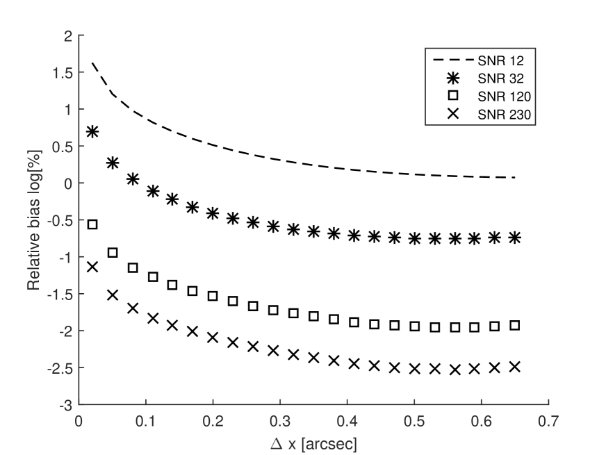
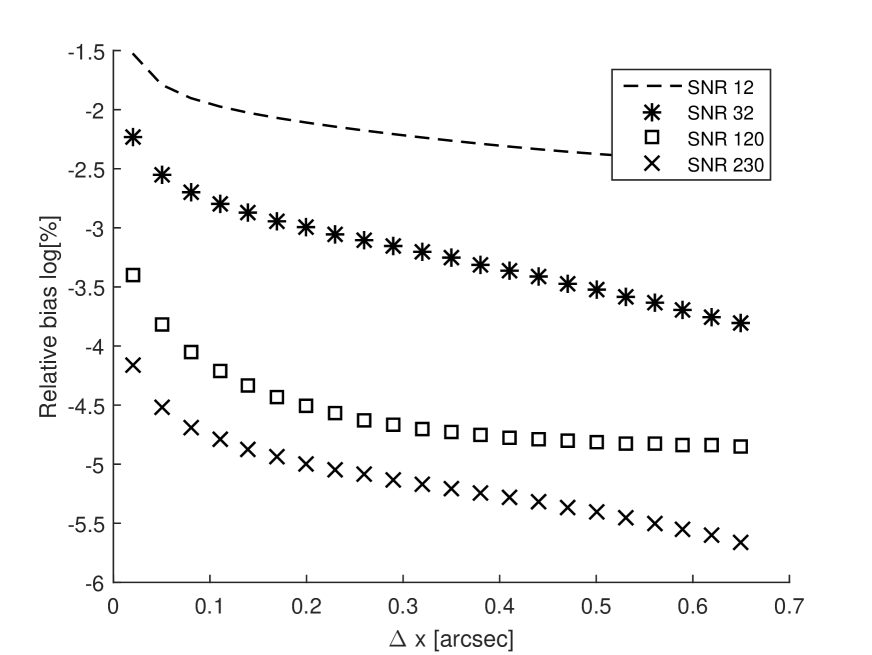
5.2 Bias analysis
Considering the upper bound terms and for the bias error obtained from Theorems 2 and 3 for the WLS and ML, respectively, Fig. 1 presents the relative bias error for different regimes and pixel resolutions. In the case of the ML estimator, the bounds for relative bias error are very small in all the explored regimes and pixel resolutions meaning that for any practical purposes this estimator is unbiased as expected from theory (Gray & Davisson, 2004). For the case of the WLS, we observe that from medium to high the relative error bound obtained is very small but, meanwhile at low , unbiasedness can not be fully guaranteed from the bound in Eq. (26). In general, our results show that both WLS and ML are unbiased estimators for astrometry in a wide range of relevant observational regimes (in particular from medium to high ) and, consequently, it is meaningful to analyze the optimality of these estimators in comparison with the CR bound in those regimes.
5.3 Performance analysis of the WLS estimator
In this section, we evaluate numerically the expression derived in Theorem 2 to bound the variance of the WLS estimator in Eq. (27). For that we characterize the admissible regime predicted for the variance of the WLS estimator, i.e., the interval
| (36) |
for and arcsec. In these bounds, we recognize its central value (or nominal value) in Eq. (28) and the length of the interval that is determined in closed form for its numerical evaluation in Eqs. (42) and (66). Note that can be considered an indicator of the precision of our result to approximate the variance of the WLS in astrometry.
5.3.1 Revisiting the uniform weight case
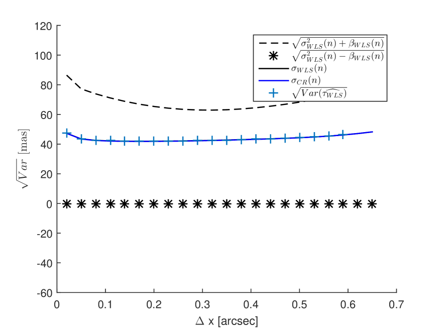
To begin the analysis, we consider the setting of uniform weights across pixels, i.e., the case of the LS estimator and, without loss of generality, we locate the object in the center of the field of view111111It is important to remind that the CR bound is a function of the value of the parameter to be estimated, in this case the position , see the Fisher information in Eq. (10)., which can be considered a reasonable scenario to represent the complexity of the astrometry task. At this point, it is important to remind the reader that from the analysis of in Remark 2, the nominal value is equivalent to the CR bound when the are selected as a function of the true position in Eq. (29). In view of this observation, the selection of non-uniform weights can be interpreted as biasing the estimation to a particular area of the angular space, which goes in contradiction with the essence of the inference problem that estimates the position with no prior information, and only relies on the measured counts. From this interpretation, revisiting the LS estimator is an important first step in the analysis of the WLS framework.
On the specifics, the boundaries of the interval in Eq. (36) and its nominal values are illustrated in Fig. 2 for the different observational regimes. In addition, Fig. 2 shows the CR bound as a reference to evaluate the optimality of the LS scheme across settings. We observe that for the low regime, the nominal values precisely match the CR bound, however our result is not conclusive as the interval around the nominal performance is significantly large. This is the regime where our result is not conclusive regarding the performance of the LS estimator. In the regime (top right panel on Fig. 2), we notice an important reduction on the range of admissible performance, and our result becomes more informative and meaningful. In this context, the nominal values is very close to the CR bound, and we could assert that the LS estimator offers sufficiently good performance in the sense that is very competitive with the MVB. Importantly, when we move to the regime of relatively high and very hight (from to ), our results are very accurate to predict the performance of the LS method, and we find that the gap between the CR and the nominal value is very significant (the deviation from the MVB is and for and at arcsec, respectively). This last result confirms one of the main findings presented in Lobos et al. (2015), who showed that for medium to high the LS estimator is suboptimal with respect to the MVB. In Fig. 2 we also show the square root of the empirical variance () with respect to the empirically-determined mean position (using the WLS estimator), all as derived from the simulations, showing good consistency with our predictions.
5.3.2 Non-uniform weight case
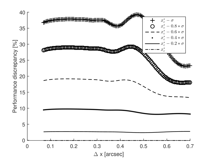
The sub-optimality of the WLS scheme from moderate to high seen in Fig. 2 can be extended for any arbitrary selection of a fixed set of weights, as it would be expected. Given that the space of weights selection is literally unlimited, we use the insight obtained from Remark 2 that states that a selection of weights can be interpreted as an specific prior on the position of the object where the optimum, but unfortunately unknown, selection (achieving the CR bound) of weights in Eq. (29) is an explicit function of the unknown position of the object. Then, we consider a finite set of positions that uniformly partition the field of view, and their corresponding weights sets , and using Eq. (29) to cover a representative collections of weights for the problem of astrometry.
Then, for a specific selection of weights in our admissible collection (attributed to a prior belief of the position of the object in the field of view), we evaluate the worse discrepancy between (which is the most favourable expression for the variance predicted from Theorem 2), and the CR bound in Proposition 1, across a collection of presumed object positions in the following range of positions
where denotes the center of the array (which, as indicated at the beginning of Sect. 5.3.1, is equal to the true object position ) and is the dispersion parameter of the PSF. The idea of using this worse case difference is justified from the fact that in this parameter estimation problem we do not know the position of the object, and consequently, the optimality of any WLS estimator should be evaluated in the worse case situation, as the scheme should be able to estimate the position of the object in any scenario (position). More precisely, for a given weight selection , we use the following worse case discrepancy
| (37) |
For this analysis note that both and are functions of the position , , and .
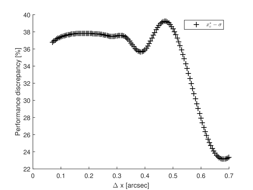
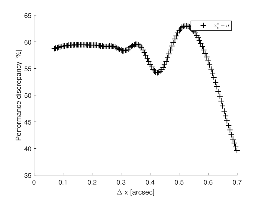
Fig. 3 illustrates the worse case discrepancy in Eq. (37) for the medium and high regimes where Theorem 2 provides an accurate and meaningful prediction of the performance of the WLS method, i.e., for , and across arcsec. The discrepancy is quite significant, on the order of and in the range for arcsec for and , respectively.
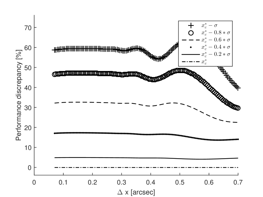
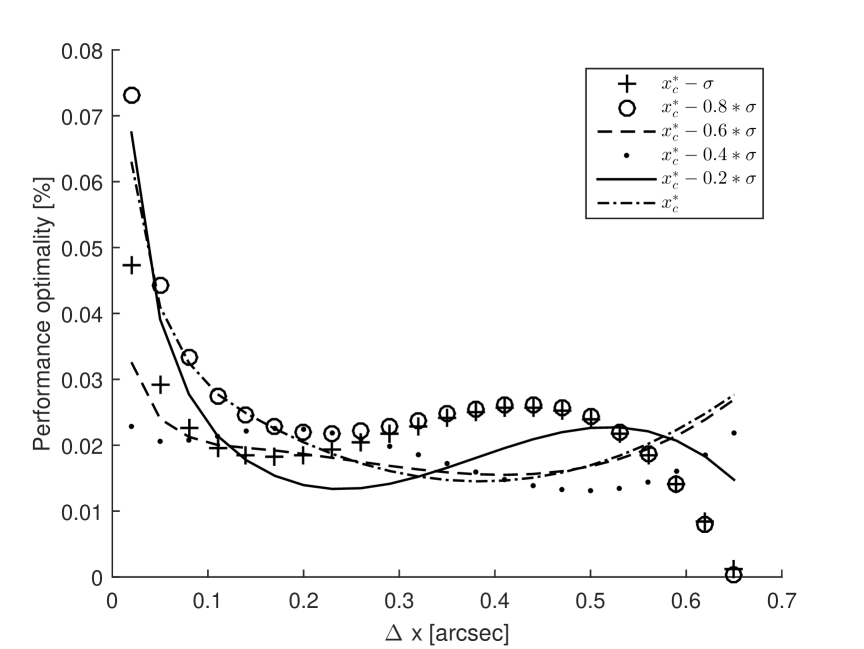
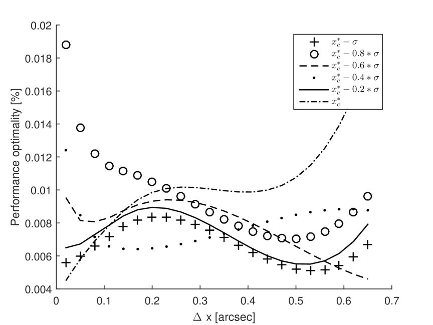
To refine the worse case analysis presented in Fig. 3, and to evaluate in more detail the sensitivity of the discrepancy indicator given by Eq. (37), we evaluate the discrepancy of WLS using the weights associated to (the center position of the array) with respect to the CR bound associated to the positions , to study how the discrepancy (measuring the non-optimality of the method) evolves when the adopted position moves far from the prior imposed by the WLS in the center of the array. Fig. 4 illustrates this behaviour, where it is possible to see that the discrepancy is very sensitive and proportional to the misassumption of the object position, where the worse case discrepancy in the maximum achievable location precision is on the order of for pixel sizes in the range arcsec for , and about for pixel sizes in the range arcsec for . These worse case scenario happens in both cases when the object is located the farthest from the prior assumption, as it would be expected.
The main conclusion derived form this CR bound analysis is that, independent of the weight selection adopted, as long as the weights are fixed, the WLS estimator is not able to achieve the CR bound in all observational regimes. More precisely, the discrepancy (measuring the non-optimality) in the less favourable case of an hypothetical and feasible position of the object is very significant, in the range of for the important regime of high and very high .
5.4 Performance analysis of the ML estimator
In this section we perform the same analysis done for the WLS in Sect. 5.3, but using the result in Theorem 3. In particular, we consider the admissible regime for the variance of the ML estimator given by
in Eq. (33), where the nominal value in this case, in Eq. (34), is precisely the CR bound, while the length of the interval is given by Eqs. (42) and (83) in closed form.
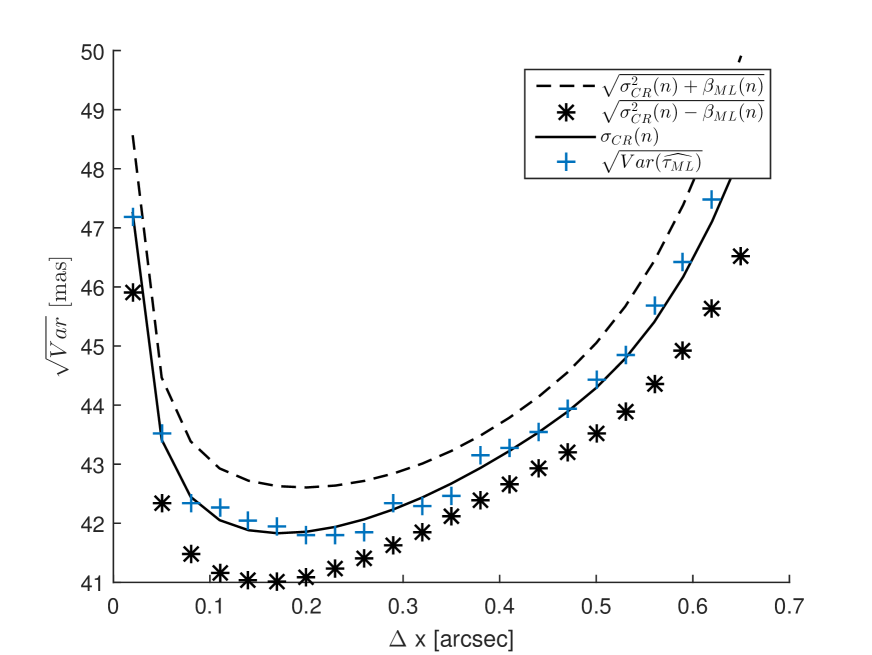
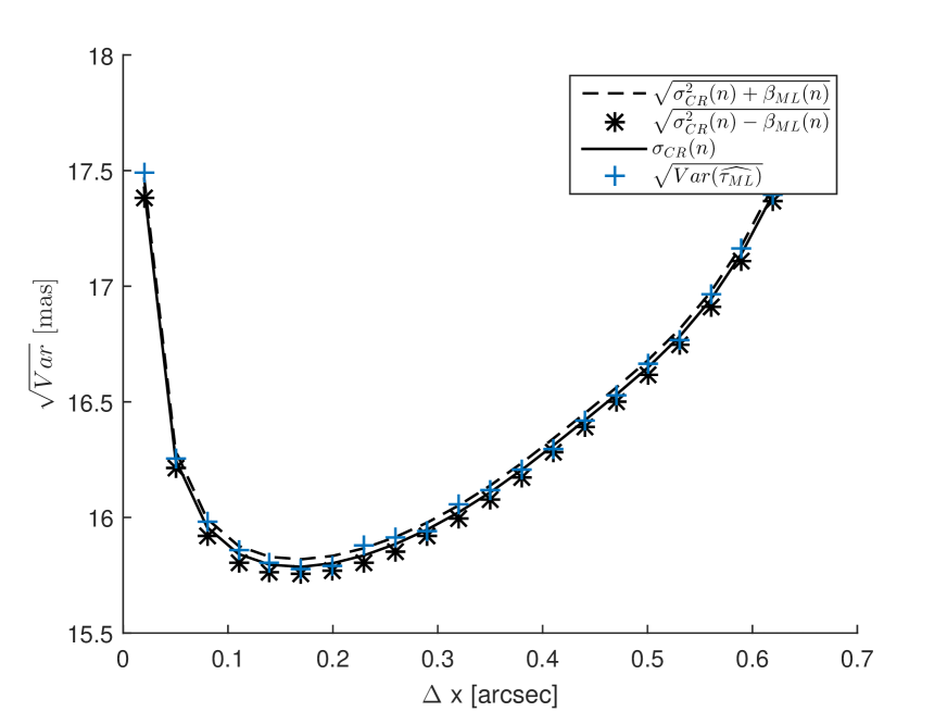
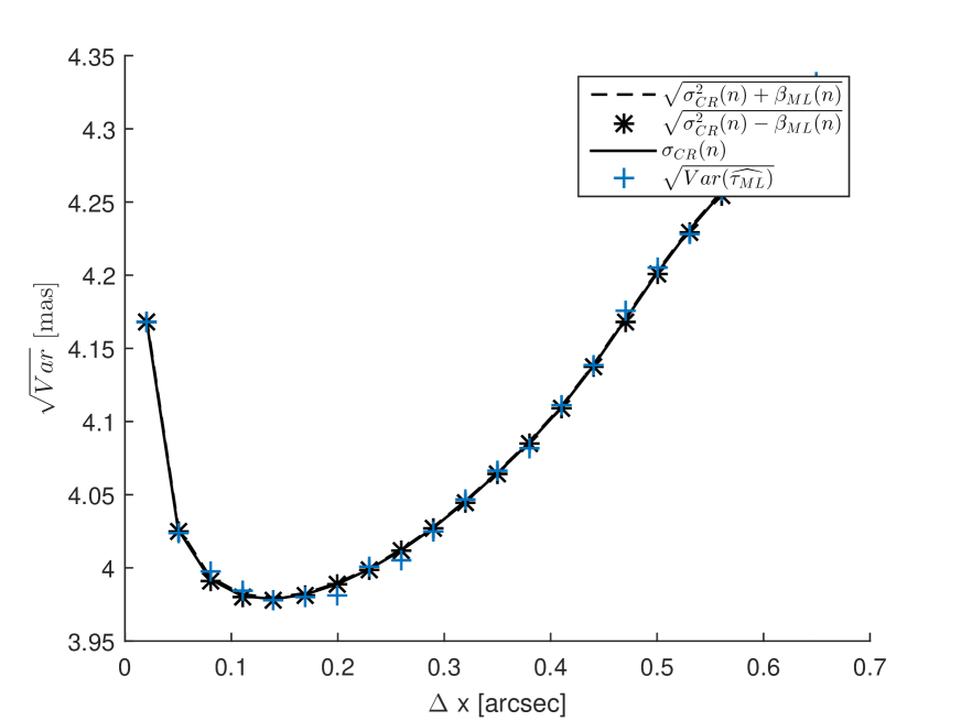
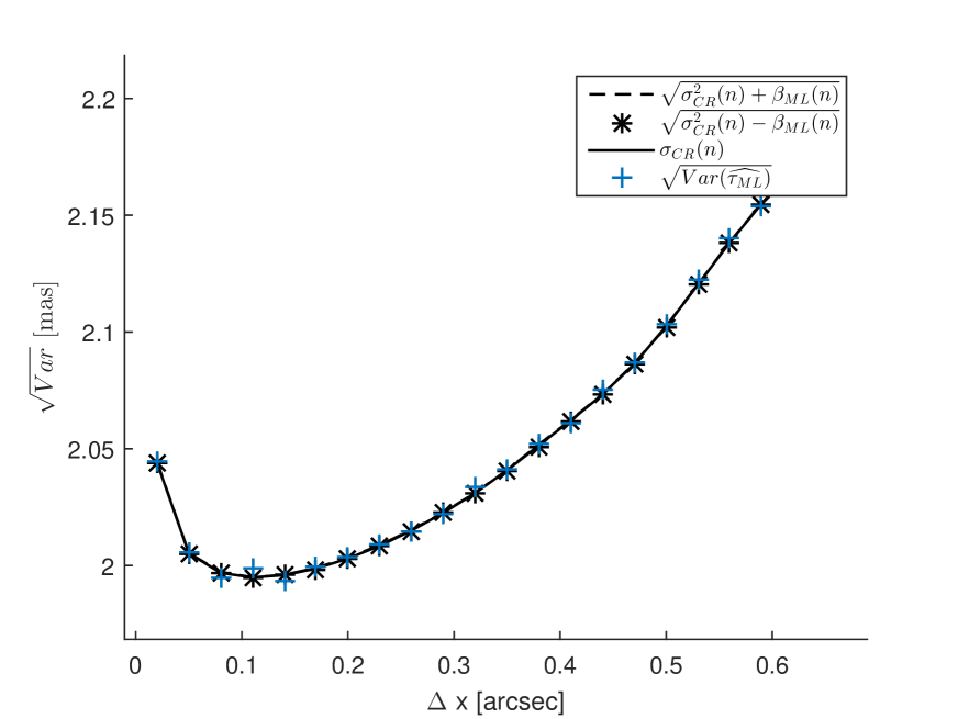
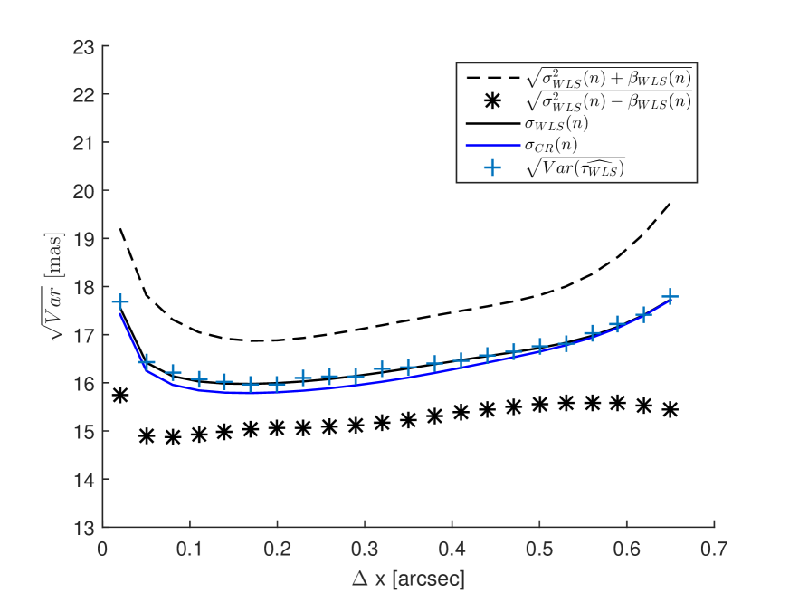
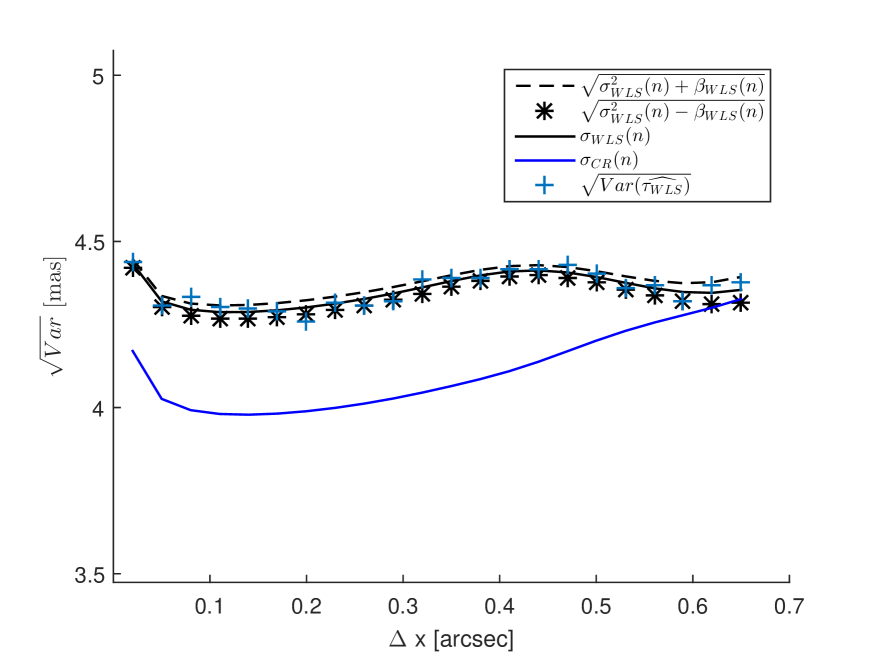
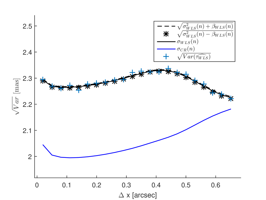
Considering an object located in the center of the array, i.e., , the performance curves are presented in Fig. 5 for and arcsec. First, we note that there is a significant difference in the predictions of our methodology for the ML estimator in comparison with what we predict in the WLS case. In fact, the results of our approach are very precise for the determination of the variance of the ML estimator in all the regimes, from small to high , which is remarkable. More important it is the fact that, from these findings, we observe that the performance deviation from the MVB in the worse case (small ) is very small (see Table 1, first row), while for any practical purposes the variance of the ML estimator achieves the CR limit for all the other regimes, from medium to high , which is a numerical corroboration of the optimality of the ML estimator in astrometry, as predicted theoretically by Theorems 1 and 3. In Fig. 5 we also show the square root of the empirical variance () with respect to the empirically-determined mean position (using the ML estimator), all as derived from the simulations, showing good consistency with our predictions.
Complementing this analysis, we conducted the same comparison considering different positions for the object within the array obtaining the same trends and conclusions. To summarize these results, Fig. 6 shows the value , which is an indicator of the quality of the estimator (the smaller the better) for different scenarios of the position of the object . In particular, for all the evaluated positions, the relative discrepancy is bounded (relative to the CR bound) by values in the range of and for pixel resolution in the range arcsec for and , respectively. Finally, Table 1 presents the relative discrepancy for all the range of values considered in this study for the case arcsec.
| Position | =12 | =32 | =120 | =230 |
|---|---|---|---|---|
| 3.8 | 0.34 | 0.032 | 0.010 | |
| 4.1 | 0.27 | 0.014 | 0.009 | |
| 4.3 | 0.19 | 0.022 | 0.007 | |
| 3.8 | 0.29 | 0.019 | 0.009 | |
| 3.9 | 0.30 | 0.022 | 0.011 | |
| 3.6 | 0.40 | 0.019 | 0.008 |
We conclude from this analysis that the ML estimator in nearly optimal for the medium, high and very high regimes across pixel resolutions, achieving the MVB for astrometry. This is an interesting result, since it lends further support to the adoption of these types of estimators for very demanding astrometric applications, as has been done in the case of Gaia (Lindegren, 2008). We note that Vakili & Hogg (2016) reach the same conclusion regarding the optimality of the ML method in comparison with the MVB, through simulations of 2D CCD images using a broad set of Moffat PSF stellar profiles. While their results are purely empirical, it is interesting that they test the ML using a different PSF from ours, and in a 2D scenario, and yet they reach the same conclusions. More recently, Gai et al. (2017) have tested (also empirically) the ML method in a 1D scenario (similar to ours), but in the context of a Gaia-like PSF. They find that the ML is unbiased (in agreement with our results, see Fig. 1), and, by comparing two implementations of the ML they conclude that they predict self-consistent and reliable results over a broad range of flux, background, and instrument response variations. It would still be quite interesting to compare the performance of those implementations against the CR MVB in order to further test our theoretical predictions.
5.5 Comments on an adaptive WLS estimator for astrometry
In Sect. 4.1 we presented results that offer a nominal prediction for the variance of the WLS method through Eq. (27) which turns out to be very accurate in the regime from medium to high as shown in Sect. 5.3. Interestingly, Remark 2 tells us that this nominal values precisely match the CR limit for an optimal selection of weights given in Eq. (29), namely for all (compare Eqs. (28) and (34)). As this selection is unfeasible, because it requires the knowledge of (see the expression in Eq. (2)), we can approximate this value by a noisy version of it, considering the fact that the expected value of the observations that we measure at pixel is using our model in Eq. (4). Therefore can be interpreted as a noisy version of and
| (38) |
can be seen as a noisy version of the ideal weight . Adopting this data-driven weighting approach, we would have an adaptive WLS method as the weights are not fixed but instead they are a function of the data . This selection of weights can be interpreted as an empirical version of the optimal weights that achieves the CR bound. Then, the problem reduces to solve
| (39) |
where
| (40) |
Fig. 7 presents the performance of this scheme for the same regimes we have been exploring in this work, supporting the conjecture that this selection of weights resembles the optimal weight selection and in fact achieves MSE performances that are surprisingly close to the CR bound in all the observational regimes.
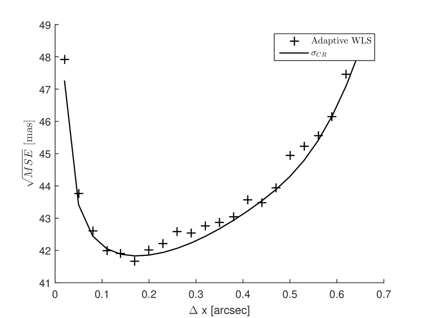
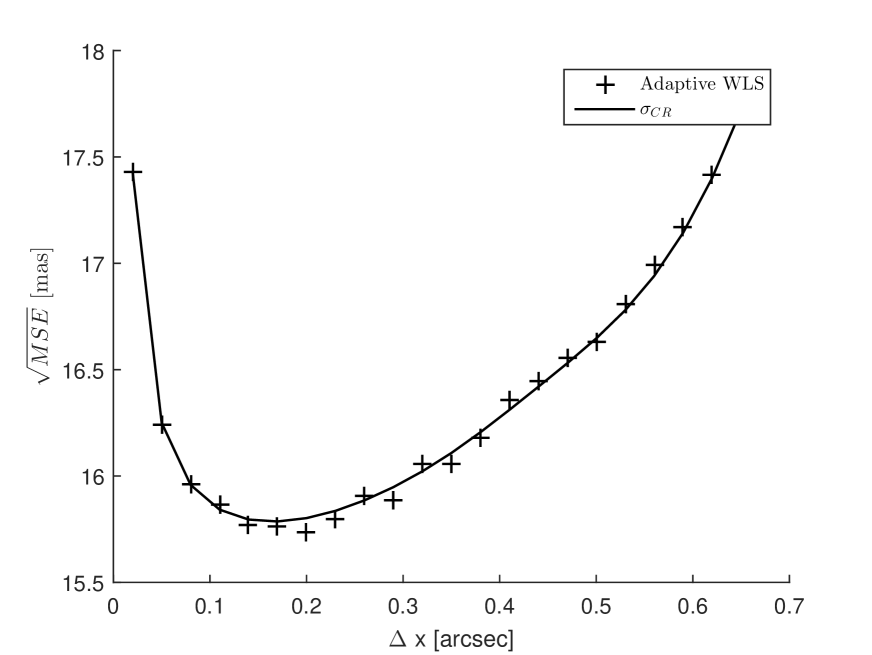
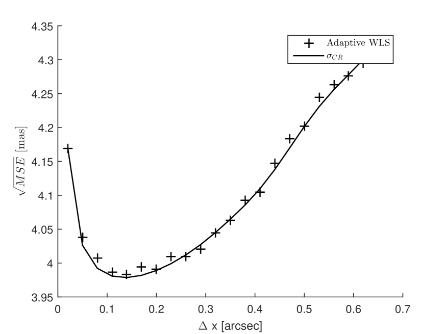
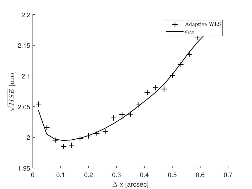
Our results in this sub-section show that some commonly adopted weighting schemes, using the analogous to Eq. (38), are a very good data-driven choice for methods that employ a WLS scheme, such is the case, e.g., of the well know PSF stellar fitting program (including astrometry) DAOPHOT, described in Stetson (1987, Eq. (10)).
5.6 Undersampled case
So far we have analyzed the performance of the ML and WLS estimators in regimes where the PSF (assumed to have a arcsec) is well sampled by the detector. In this section we analyze the undersampled case, where we have only a few pixels that capture most the flux of the source. This scenario would be typical of nearly diffraction-limited images taken, e.g., from the space, or with an AO system from the ground.
Table 2 shows the performance of the bounds presented in Theorems 2 and 3 in the undersampled regime, where the PSF is concentrated in only a few pixels (order of 5 to 9 pixels), and where the flux is relatively large. For the space-based case, the background is reduced almost to the purely instrument noise (left numbers in the table), while in the ground-based case the background would be larger, but we would still have a very large Strehl ratio. From the table it can be seen that the performance is nearly optimal with the ML estimator, even in the severely undersampled regime (small FWHM values). On the other hand, the WLS deteriorates its performance very quickly as the image size decreases, reaching up to nearly 45% when the FWHM is on the order of the detector pixel size.
| FWHM | ML error [] | WLS error [] |
|---|---|---|
| 0.03 / 0.02 | 25 / 45 | |
| 0.03 / 0.02 | 5.5 / 8.0 | |
| 0.01 / 0.03 | 1.9 / 2.8 | |
| 0.01 / 0.04 | 1.4 / 2.3 |
We emphasize that the above results are computed in the ideal situation of a uniform pixel response function (and a perfect flat-field correction), whereas in reality a non-uniform pixel response has a critical impact on the Cramér-Rao bound as demonstrated by Adorf (1996, Figure 1). In addition, in the case of stare-mode space-based images acquired under very small background, charge transfer inefficiency effects due to time-varying charge-traps in the detector would also blur (and systematically shift) the images, deteriorating the ultimate astrometric precision above the Cramér-Rao limit (for details, see, e.g., Bristow et al. (2006), especially their Figure 10).
6 Summary, conclusions, and outlook
In this paper we study the performance of the WLS and ML estimators for relative astrometry on digital detectors subject to Poisson noise, in comparison with the best possible attainable precision given by the CR bound. Our study includes analytical results, and numerical simulations under realistic observational conditions to help us to corroborate our theoretical findings.
By generalizing the proposal by Fessler (1996) we are able to obtain, for the first time, close-form expressions for the variance and the mean of implicit estimators (as is the particular case of the WLS and ML schemes), which can be computed directly from the data (see Theorem 1, in particular Eqs. (21) and (22), and Appendix A). When specifying this result to astrometry with digital detectors, we are able to bound both the bias and the variance of the relative position of a celestial source on a CCD array as a function of all the relevant parameters of the problem (see Eqs. (26) and (27) or Eqs. (32) and (33) for the WLS and ML estimators respectively). We verified that the bias of the WLS and ML methods are negligible in all the observational regimes explored in this paper (see Fig. 1).
A careful analysis of our predictions confirms earlier results by Lobos et al. (2015) (for the LS method) in that the WLS method is, in general, sub-optimal (in comparison with the MVB given by the CR result), specially at high and very high (see the two bottom panels on Fig. 2). However, a judicious data-driven selection of weights (called “adaptive” WLS method by us, Sect. (5.5)), improves the performance of the WLS substantially (see Fig. 7). This is an interesting result, given the widespread use and simple numerical implementation of the WLS method.
The ML method is found to have both a smaller bias than the WLS method (compare left and right panels of Fig. 1), although the bias on both methods is already quite small, and a tight correspondence to the MVB throughout the entire range of regimes explored in this paper (Fig. 5). Therefore, the ML estimator for astrometry is consistently optimal, and should be the estimator of choice for high-precision applications.
This paper, along with Lobos et al. (2015), completes an in-depth study of the performance of commonly used estimators in astrometry using PIDs, and sets the stage for the development of codes that could efficiently implement astrometric ML estimators on 2D detectors, incorporating also the simultaneous measurement of fluxes, as explored by Gai et al. (2017).
7 Acknowledgments
SE acknowledges support from CONICYT-PCHA/MagisterNacional/2016 - 22160840. The authors want to thank the support of the Advanced Center for Electrical and Electronic Engineering, AC3E, Basal Project FB0008, PIA ACT1405, and the Chilean Centro de Excelencia en Astrofisica y Tecnologias Afines (CATA) BASAL PFB/06 from CONICYT. The authors also acknowledge support by CONICYT/FONDECYT grants # 1151213, 1170044, and 1170854. RAM also acknowledges support from the Project IC120009 Millennium Institute of Astrophysics (MAS) of the Iniciativa Cientifica Milenio del Ministerio de Economia, Fomento y Turismo de Chile. Finally, we thank an anonymous referee for his/her careful reading of our manuscript, and for pointing out the exploration of the relevant space-based undersampled regime that led to the discussion in Section 5.6.
Appendix A Proof of Theorem 1
We begin presenting the expressions for to complete the statement of the result.
| (41) |
| (42) |
where
| (43) |
| (44) |
and, finally,
| (45) |
Proof of Theorem 1: Using the chain rule in the cost function and taking the partial derivative of both sides in (15), we have that
| (46) |
Thus, we have equations with one unknown, and it holds for any . Defining the operators
| (47) |
of dimensions and , respectively, we can express (46) in matrix form as
| (48) |
Assuming that the matrix is non singular, we can calculate from (48)
| (49) |
Finally, using (49), evaluating at , and then replacing in (18), we have that
| (50) | |||||
Moving into the residual term in (18) captured by , we must consider the variance of the error function and the covariance . For the first, we have that
| (51) | |||||
On the other hand, for the covariance, using the main assumption in (19), it is clear that
| (52) |
From this,
| (53) | |||||
Finally, replacing (51) and (53) in the definition of , we have that:
| (54) | |||||
For the bias expression of the result in (21), using the hypothesis in (20), we can take expectation at both sides of (17) to obtain that
| (55) |
Appendix B Proof of Theorem 2
Proof: The proof and, in particular, the derivation of , and simply reduces to an straightforward application of Theorem 1. For that we need to first validate the assumptions of Theorem 1. If we begin with Eq. (49)
| (56) |
and then we calculate the gradient terms in the RHS of (56) for our WLS context, it follows that
| (57) | |||||
| (58) | |||||
| (59) |
Following (56), we need to evaluate Eqs. (57) and (59) at . For that, we have the following121212considering that .
| (60) |
Then we will use the following result:
Proposition \thetheorem
Under the assumption of a Gaussian PSF, .
Notice that this proposition is the second assumption used in Theorem 1. Using this proposition, we obtain that
| (61) | |||||
| (62) | |||||
Finally, applying (61) and (62) in (49) we have that
| (63) | |||||
which offers the decomposition needed for the application of Theorem 1 (Eq. (19)). For the value of in (45), since the observations are independent and follow a Poisson distribution, we have that
| (64) |
Then if we replace (61), (62) and (64) in (45), we have that
| (65) |
On the other hand, the expression for and can be determined from the evaluation of (42) and (41), respectively. Looking at them, the problem reduces to determine the key term . For that, if we use (Fessler, 1996, Eq. (17)) we can obtain the following identity131313The derivation of this identity is presented in Appendix B.2.
| (66) |
which concludes the result.
B.1 Proof of Proposition 2
Proof: Using the function , we need to show that the minimum is reached only at . From this, we have that and it achieves its minimum at . To prove uniqueness, let us assume that there is another position at which is zero. Then
| (67) | |||||
The last identity is not possible, because if we use a Gaussian PSF there is at least one such that .
B.2 Proof of Eq. (66)
Proof: Recall (Fessler, 1996, Eq. (17)) and considering as the cost function we have that
| (68) |
where from the definition of we have that
| (69) |
| (70) |
| (71) |
| (72) |
Concerning it is just the -th component of the gradient in Eq. (56), then we use (57) and (59)
| (73) |
Finally, replacing (69), (70), (71), (72) and (73) in (68), and evaluating in we obtain the desired result
| (74) |
Appendix C Proof of Theorem 3
Proof: Again the proof and the derivation of , and reduce to apply Theorem 1. First, we need to validate the assumption of Theorem 1. Beginning with the equality in Eq. (56), it follows that
| (75) | |||||
| (76) | |||||
For evaluating these two expression at as required in (56), we use that141414Considering that .
| (77) |
Then we will use the following result
Proposition \thetheorem
Under the assumption of a Gaussian PSF, .
Notice again, that this proposition is the second assumption used in Theorem 1. From this proposition, it follows that
| (78) | |||||
| (79) | |||||
Finally, we apply (78) and (79) in (49) to obtain that
| (80) | |||||
that shows that the sufficient condition in (19) of Theorem 1 is satisfied. For computing the value in (45), we have that
| (81) |
since the observations are independent and follow a Poisson distribution. Then, replacing (78), (79) and (81) in (45) we have that
| (82) |
which resolves the identity in (34). Finally and comes from evaluating (42) and (41) in this ML context. For that we only need to determine . Using (Fessler, 1996, Eq. (17)), we can obtain the following identity151515The derivation of this result is presented in Appendix C.2.
| (83) |
which concludes the result.
C.1 Proof of Proposition 3
Proof: Let us consider the function given by
| (84) |
We note that
| (85) |
where applying first order condition , . Returning to our problem in (77) where and , it is clear, considering the Gaussian profile in PSF, that
| (86) |
which concludes the result.
C.2 Proof of Eq. (83)
Proof: Recall (Fessler, 1996, Eq. (17)) and considering as the cost function we have that:
| (87) |
where from the definition of we have that
| (88) |
| (89) |
| (90) |
| (91) |
Concerning it is just the -th component of the gradient in Eq. (56), then we use (75) and (76)
| (92) |
Finally, replacing (88), (89), (90), (91) and (92) in (87), and evaluating in we obtain the desired result
| (93) |
References
- Adorf (1996) Adorf, H.-M. 1996, in Astronomical Data Analysis Software and Systems V, Vol. 101, 13
- Alard & Lupton (1998) Alard, C. & Lupton, R. H. 1998, The Astrophysical Journal, 503, 325
- Altmann et al. (2014) Altmann, M., Bouquillon, S., & Taris, F. 2014, in Proc. SPIE, Vol. 9149, 91490P
- Auer & Van Altena (1978) Auer, L. & Van Altena, W. 1978, The Astronomical Journal, 83, 531
- Bastian (2004) Bastian, U. 2004, GAIA technical note, 2004 BASNOCODE
- Bendinelli et al. (1987) Bendinelli, O., Parmeggiani, G., Piccioni, A., & Zavatti, F. 1987, The Astronomical Journal, 94, 1095
- Benedict et al. (2016) Benedict, G. F., McArthur, B. E., Nelan, E. P., & Harrison, T. E. 2016, Publications of the Astronomical Society of the Pacific, 129, 012001
- Bouquillon et al. (2017) Bouquillon, S., Mendez, R., Altmann, M., et al. 2017, Astronomy & Astrophysics, 606, A27
- Bradley & Gart (1962) Bradley, R. A. & Gart, J. J. 1962, Biometrika, 49, 205
- Bristow et al. (2006) Bristow, P., Kerber, F., & Rosa, M. 2006, in The 2005 HST Calibration Workshop: Hubble After the Transition to Two-Gyro Mode, 299
- Cacciari et al. (2016) Cacciari, C., Pancino, E., & Bellazzini, M. 2016, Astronomische Nachrichten, 337, 899
- Chromey (2016) Chromey, F. R. 2016, To measure the sky: an introduction to observational astronomy (Cambridge University Press)
- Chun-Lin (1993) Chun-Lin, L. 1993, in Symposium-International Astronomical Union, Vol. 156, Cambridge University Press, 113–116
- Cover & Thomas (2012) Cover, T. M. & Thomas, J. A. 2012, Elements of information theory (John Wiley & Sons)
- Cramér (1946) Cramér, H. 1946, Scandinavian Actuarial Journal, 1946, 85
- Echeverria et al. (2016) Echeverria, A., Silva, J. F., Mendez, R. A., & Orchard, M. 2016, Astronomy & Astrophysics, 594, A111
- Fessler (1996) Fessler, J. A. 1996, IEEE Transactions on Image Processing, 5, 493
- Gai et al. (2017) Gai, M., Busonero, D., & Cancelliere, R. 2017, Publications of the Astronomical Society of the Pacific, 129, 054502
- Gray & Davisson (2004) Gray, R. M. & Davisson, L. D. 2004, An introduction to statistical signal processing (Cambridge University Press)
- Hoadley (1971) Hoadley, B. 1971, The Annals of mathematical statistics, 1977
- Høg (2017) Høg, E. 2017, arXiv preprint arXiv:1707.01020
- Howell (2006) Howell, S. B. 2006, Handbook of CCD astronomy, Vol. 5 (Cambridge University Press)
- Jakobsen et al. (1992) Jakobsen, P., Greenfield, P., & Jedrzejewski, R. 1992, Astronomy and astrophysics, 253, 329
- Janesick (2001) Janesick, J. R. 2001, Scientific charge-coupled devices, Vol. 83 (SPIE press)
- Janesick (2007) Janesick, J. R. 2007, Photon transfer (SPIE press San Jose)
- Kay (1993) Kay, S. M. 1993, Fundamentals of statistical signal processing. Vol 1, Estimation theory
- Kendall et al. (1999) Kendall, M., Stuart, A., Ord, J., & Arnold, S. 1999, Arnold [etc.], London [etc.]
- King (1971) King, I. R. 1971, Publications of the Astronomical Society of the Pacific, 83, 199
- King (1983) King, I. R. 1983, Publications of the Astronomical Society of the Pacific, 95, 163
- Lattanzi (2012) Lattanzi, M. 2012, Mem. SA It, 83, 1033
- Lee & Van Altena (1983) Lee, J.-F. & Van Altena, W. 1983, The Astronomical Journal, 88, 1683
- Lemon et al. (2017) Lemon, C. A., Auger, M. W., McMahon, R. G., & Koposov, S. E. 2017, Monthly Notices of the Royal Astronomical Society, 472, 5023
- Lindegren (1978) Lindegren, L. 1978, in International Astronomical Union Colloquium, Vol. 48, Cambridge University Press, 197–217
- Lindegren (2008) Lindegren, L. 2008, Gaia DPAC public document GAIA-C3-TN-LU-LL-078 (November 2008)
- Lindegren (2010) Lindegren, L. 2010, ISSI Scientific Reports Series, 9, 279
- Lobos et al. (2015) Lobos, R. A., Silva, J. F., Mendez, R. A., & Orchard, M. 2015, Publications of the Astronomical Society of the Pacific, 127, 1166
- McLean (2008) McLean, I. S. 2008, Electronic imaging in astronomy: detectors and instrumentation (Springer Science & Business Media)
- Méndez et al. (2010) Méndez, R. A., Costa, E., Pedreros, M. H., et al. 2010, Publications of the Astronomical Society of the Pacific, 122, 853
- Mendez et al. (2013) Mendez, R. A., Silva, J. F., & Lobos, R. 2013, Publications of the Astronomical Society of the Pacific, 125, 580
- Mendez et al. (2014) Mendez, R. A., Silva, J. F., Orostica, R., & Lobos, R. 2014, Publications of the Astronomical Society of the Pacific, 126, 798
- Michalik & Lindegren (2016) Michalik, D. & Lindegren, L. 2016, Astronomy & Astrophysics, 586, A26
- Michalik et al. (2015) Michalik, D., Lindegren, L., Hobbs, D., & Butkevich, A. G. 2015, Astronomy & Astrophysics, 583, A68
- Prusti et al. (2016) Prusti, T., De Bruijne, J., Brown, A. G., et al. 2016, Astronomy & Astrophysics, 595, A1
- Rao (1945) Rao, C. R. 1945, Bull. Calcutta Math. Soc., 37, 81
- Reffert (2009) Reffert, S. 2009, New Astronomy Reviews, 53, 329
- So et al. (2013) So, H. C., Chan, Y. T., Ho, K., & Chen, Y. 2013, IEEE Signal Processing Magazine, 30, 162
- Stetson (1987) Stetson, P. B. 1987, Publications of the Astronomical Society of the Pacific, 99, 191
- Stone (1989) Stone, R. C. 1989, The Astronomical Journal, 97, 1227
- Vakili & Hogg (2016) Vakili, M. & Hogg, D. W. 2016, arXiv preprint arXiv:1610.05873
- Van Altena (2013) Van Altena, W. F. 2013, Astrometry for astrophysics: methods, models, and applications (Cambridge University Press)
- Van Altena & Auer (1975) Van Altena, W. F. & Auer, L. 1975, in Image Processing Techniques in Astronomy (Springer), 411–418
- Van Trees (2004) Van Trees, H. L. 2004, Detection, estimation, and modulation theory, part I: detection, estimation, and linear modulation theory (John Wiley & Sons)
- Zaccheo et al. (1995) Zaccheo, T., Gonsalves, R., Ebstein, S., & Nisenson, P. 1995, The Astrophysical Journal, 439, L43
- Zhang et al. (2016) Zhang, J., Hao, Y. C., Wang, L., & Long, Y. 2016, Publications of the Astronomical Society of the Pacific, 128, 035003