Exact Lexicographic Scheduling and Approximate Rescheduling

Supplementary Material for “Exact Lexicographic Scheduling and Approximate Rescheduling”

Abstract

In industrial resource allocation problems, an initial planning stage may solve a nominal problem instance and a subsequent recovery stage may intervene to repair inefficiencies and infeasibilities due to uncertainty, e.g. machine failures and job processing time variations. In this context, we investigate the minimum makespan scheduling problem, a.k.a. $P||C_{\max}$, under uncertainty. We propose a two-stage robust scheduling approach where first-stage decisions are computed with exact lexicographic scheduling and second-stage decisions are derived using approximate rescheduling. We explore recovery strategies accounting for planning decisions and constrained by limited permitted deviations from the original schedule. Our approach is substantiated analytically, with a price of robustness characterization parameterized by the degree of uncertainty, and numerically. This analysis is based on optimal substructure imposed by lexicographic optimality. Thus, lexicographic optimization enables more efficient rescheduling. Further, we revisit state-of-the-art exact lexicographic optimization methods and propose a lexicographic branch-and-bound algorithm whose performance is validated computationally.

1 Introduction

Motivated by industrial resource allocation problems, we consider scheduling under uncertainty, e.g. a machine may unexpectedly fail, a client may suddenly cancel a job, or jobs are completed earlier than expected. We focus on robust scheduling, i.e. hedge against worst-case realizations of imprecise parameter values, such as job processing times and number of available machines, lying in well-defined uncertainty sets [5, 8, 26, 56]. Because static robust optimization may produce conservative solutions compared to ones obtained with perfect knowledge [54], we investigate two-stage robust optimization with recovery [6, 9, 10, 31, 36]. As shown in Figure 1, (i) an initial planning stage computes a solution with nominal parameter values and (ii) a subsequent recovery stage modifies the solution once the uncertainty is realized, i.e. after the final parameter values become known.

We elaborate on the fundamental makespan scheduling problem, a.k.a. $P||C_{\max}$ [15, 27, 35]. With perfect knowledge, an instance $I$ of the problem posits a set $\mathcal{J}$ of jobs, each one associated with processing time $p_{j}$, a set $\mathcal{M}$ of parallel identical machines and the objective is to construct a non-preemptive schedule $S$ of minimum makespan $C_{\max}=\max_{i\in\mathcal{M}}\{C_{i}\}$, i.e. maximum machine completion time. In a two-stage setting under uncertainty, the planning stage solves a nominal instance $I_{init}$ producing a solution $S_{init}$ and the recovery stage transforms schedule $S_{init}$ to a new schedule $S_{new}$ for $I_{new}$ by repairing inefficiencies and infeasibilities, e.g. due to job processing time variations and machine failures, as illustrated in Figure 2.

In the extreme case, the recovery stage may solve $I_{new}$ from scratch without accounting for the first-stage decisions in $S_{init}$. This level of flexibility may sacrifice benefits due to planning and can be resource-consuming. For example, significantly modifying machine schedules may incur substantial communication costs in distributed computing [57]. To mitigate this overhead, we only allow a bounded number of modifications to $S_{init}$. Technically, we distinguish between binding and free optimization decisions. Binding decisions are variable evaluations determined from the initial solution after uncertainty realization. Free decisions are variable evaluations that cannot be determined from the initial solution, but are essential to ensure feasibility. For instance, scheduling a job with a modified processing time is a binding decision because the planning stage already specifies an assignment. Assigning a new job after uncertainty realization is a free decision because no assignment is given in the planning stage. Further, we study rescheduling with limited binding decision modifications and thereby stay close to the initial solution. By allowing few modifications, first-stage decisions remain critical.

Figure 1: Recoverable robustness setting

Figure 2: Makespan recovery problem

A two-stage robust optimization method should specify (i) a way of producing the initial solution $S_{init}$, and (ii) a recovery strategy for restoring $S_{init}$ and deriving the recovered solution $S_{rec}$, after uncertainty realization. Analyzing a two-stage robust optimization method requires defining (i) the uncertainty set of the problem, and (ii) the investigated performance guarantee.

Uncertainty Set

The uncertainty set of a robust optimization problem specifies a range of possible values for the uncertain parameters [33]. We consider a generalization of well-known $\Gamma$-uncertainty sets, where the final parameter values $\hat{p}_{j}$ vary in an interval $[p_{j}^{L},p_{j}^{U}]$ and at most $k$ parameters can deviate from their nominal values [11]. Here, the uncertainty set is defined by a pair $(k,f)$, where $k$ is the maximum number of unstable parameters with respect to perturbation factor $f>1$. A parameter $p_{j}>0$ is stable if $p_{j}/f\leq\hat{p}_{j}\leq fp_{j}$ and unstable, otherwise.

Performance Guarantee

Theoretical performance guarantees are useful for determining when robust optimization methods are efficient [8, 26]. Denote by $C(I_{new})$ the cost, e.g. makespan, of a solution obtained by some robust optimization method and by $C^{*}(I_{new})$ the cost of an optimal solution obtained with perfect knowledge [40]. We consider the so-called price of robustness which is defined as the ratio between the two and seek a tight, worst-case performance guarantee $\rho=\max_{I_{new}\in\mathcal{I}}(C(I_{new})/C^{*}(I_{new}))$ within the set $\mathcal{I}$ of all problem instances [12].

Related Work

Prior literature shows that scheduling problems become computationally harder after incorporating uncertainty [28, 29, 56]. Kasperski & Zielinski [32] survey techniques and negative results for robust scheduling, including $P||C_{\max}$ with uncertain job processing times. Typically, robustness is achieved by optimizing the worst-case (i) cost or (ii) distance from the achievable optimum with perfect knowledge, over all scenarios in the uncertainty set. These robust counterparts of standard deterministic optimization problems are often referred to as minmax and minmax regret, respectively [33].

With perfect knowledge, $P||C_{\max}$ is strongly $\mathcal{NP}$-hard, but admits greedy constant-factor approximation algorithms and polynomial-time approximation schemes (PTASs) [15, 35]. When the number of machines is constant, $Pm||C_{\max}$ is weakly $\mathcal{NP}$-hard and has fully polynomial-time approximation schemes. With budgeted uncertainty, where $B$ bounds the deviation of the sum of processing times from their nominal values, minmax $P||C_{\max}$ admits a PTAS when $B$ is constant and a 3-approximation algorithm for arbitrary $B$ [13].

To our knowledge, no prior work analyzes the price of robustness for $P||C_{\max}$ under uncertainty. Determining the price of robustness for fundamental combinatorial optimization problems has been repeatedly posed as an open question by domain experts [8, 12, 26]. The current manuscript shows that such an analysis provides useful structural properties and quantifies the effect of uncertainty in robust solutions for $P||C_{\max}$.

Lexicographic Optimization

LexOpt is at the core of our two-stage scheduling approach. LexOpt is a subclass of multiobjective optimization minimizing $m$ objective functions $F_{1},\ldots,F_{m}:\mathcal{S}\rightarrow\mathbb{R}_{0}^{+}$, in decreasing priority order [21, 45]. In other words, LexOpt optimizes the highest-rank objective $F_{1}$, then the second most important objective $F_{2}$, then the third $F_{3}$, etc.:

$$\text{lex}\min\{F_{1}(S),\ldots,F_{m}(S):S\in\mathcal{S}\}.$$ (LexOpt)

There are indications that LexOpt is useful in optimization under uncertainty. LexOpt maintains a good approximate schedule when jobs are added and deleted dynamically [48, 53]. LexOpt is also useful for cryptographic systems against attacks [58]. We consider the LexOpt scheduling problem $\text{lex}\min\{C_{1}(S),\ldots,C_{m}(S):S\in\mathcal{S}\}$ of computing a schedule $S$ with lexicographically minimal machine completion times and show that it enables more efficient two-stage robust scheduling. That is, we identify robust scheduling as a new LexOpt application.

Apart from optimization under uncertainty, designing efficient LexOpt methods is motivated by LexOpt applications: equitable allocation of a divisible resource [25, 37], fairness [14], and exploiting opponent mistakes in game theory [42, 50]. Solution strategies include sequential, weighting, and highest-rank objective methods [16, 19, 21, 44, 45, 51, 52]. There is work characterizing the convex hull of LexOpt problems [1, 30, 41]. Logic-based methods are also applicable [38].

Contributions and Paper Organization

Our main contribution is a two-stage robust scheduling approach for $P||C_{\max}$ under uncertainty, where first-stage decisions are computed with mixed-integer linear programming and lexicographic optimization, while second-stage decisions are derived using approximation algorithms. Despite the relevant literature on two-stage robust optimization for various applications [6, 17, 18, 36], we are not aware of any work on cornerstone scheduling problems, such as $P||C_{\max}$, combined with a price of robustness characterization.

The manuscript proceeds as follows. Section 2 formally defines $P||C_{\max}$, LexOpt scheduling, and the considered perturbation types. Section 3 develops a branch-and-bound algorithm for the LexOpt scheduling problem. Section 4 proposes a recovery strategy and analyzes the performance of the overall two-stage approach theoretically. Section 5 substantiates the branch-and-bound method with respect to state-of-the-art LexOpt approaches adapted to LexOpt scheduling. Further, Section 5 validates our two-stage method empirically. Section 6 concludes.

After proving that the makespan recovery problem is strongly $\mathcal{NP}$-hard, at least as hard as solving the problem with full input knowledge, we elaborate on performance guarantees for two-stage $P||C_{\max}$ under uncertainty. Technically, we investigate a basic recovery strategy that enforces all available binding decisions and performs only essential actions to regain feasibility. On the negative side, every recovered solution is a weak approximation if planning produces an arbitrary nominal optimal solution. Specifically, every recovered solution attains an $\Omega(m)$ price of robustness, even in the case of a single perturbation. On the positive side, we obtain significantly better performance guarantees if the initial solution is LexOpt. For a single perturbation, planning using LexOpt ensures a price of robustness equal to 2. For multiple perturbations, the initial solution can be weakly reoptimizable with a high-degree of uncertainty. However, we show an asymptotically tight $O(f(1+\frac{k}{m-k})(f+k)(1+\frac{\delta}{m}))$ price of robustness, where $k$ is the number of unstable jobs with respect to a perturbation factor $f$ and $\delta/m$ is the fraction of additional machines, after uncertainty realization. This result exploits our uncertainty set structure. Therefore, when $k$, $f$ and $\delta/m$ are constant, our approach achieves an $O(1)$ price of robustness.

The main paper includes the proof of Theorem 3 and part of the proofs for Theorems 4-5, which bound the price of robustness of our two-stage robust scheduling approach for $P||C_{max}$ under uncertainty in the case of single and multiple perturbations, respectively, by exploiting the optimal substructure imposed by LexOpt. All remaining proofs are provided in the supplementary material.

2 Problem Definitions

This section defines the $P||C_{\max}$ problem (Section 2.1), the LexOpt scheduling problem (Section 2.2), and describes the investigated perturbations (Section 2.3).

2.1 Makespan Scheduling Problem

An instance $I$ of the makespan scheduling problem, a.k.a. $P||C_{\max}$, is a pair $(m,\mathcal{J})$, where $\mathcal{J}=\{J_{1},\ldots,J_{n}\}$ is a set of $n$ jobs, with processing times $p_{1},\ldots,p_{n}$, to be executed by a set $\mathcal{M}=\{M_{1},\ldots,M_{m}\}$ of $m$ parallel identical machines. Job $J_{j}\in\mathcal{J}$ must be processed by exactly one machine $M_{i}\in\mathcal{M}$ for $p_{j}$ units of time non-preemptively, i.e. in a single continuous interval without interruptions. Each machine processes at most one job per time. The objective is to minimize the last machine completion time. Given a schedule $S$, let $C_{\max}(S)$ and $C_{i}(S)$ be the makespan and the completion time of machine $M_{i}\in\mathcal{M}$, respectively, in $S$. In the following mixed-integer linear programming (MILP) formulation, binary variable $x_{i,j}$ is 1 if job $J_{j}\in\mathcal{J}$ is executed by machine $M_{i}\in\mathcal{M}$ and 0, otherwise.

$$\min_{C_{\max},C_{i},x_{i,j}}\quad C_{\max}$$ (1a)

$$C_{\max}\geq C_{i} M_{i}\in\mathcal{M}$$ (1b)

$$C_{i}=\sum_{j=1}^{n}x_{i,j}\cdot p_{j} M_{i}\in\mathcal{M}$$ (1c)

$$\sum_{i=1}^{m}x_{i,j}=1 J_{j}\in\mathcal{J}$$ (1d)

$$x_{i,j}\in\{0,1\} J_{j}\in\mathcal{J},M_{i}\in\mathcal{M}.$$ (1e)

Expression (1a) minimizes makespan. Constraints (1b) enforce that $C_{\max}=\max_{1\leq i\leq m}\{C_{i}\}$. Constraints (1c) ensure that a machine executes at most one job per time. Constraints (1d) impose that each job is assigned to exactly one machine.

2.2 LexOpt Scheduling Problem

The problem $\text{lex}\min\{F_{1}(S),\ldots,F_{m}(S):S\in\mathcal{S}\}$ minimizes $m$ objective functions $F_{1},\ldots,F_{m}:\mathcal{S}\rightarrow\mathbb{R}_{0}^{+}$ over a set $\mathcal{S}$ of feasible solutions. The functions are sorted in decreasing priority order, i.e. $F_{i}$ is more important than $F_{i^{\prime}}$, for $i<i^{\prime}$. In a LexOpt solution $S^{*}$, $F_{1}(S^{*})=v_{1}^{*}=\min\{F_{1}(S):S\in\mathcal{S}\}$ and $F_{i}(S^{*})=v_{i}^{*}=\min\{F_{i}(S):S\in\mathcal{S},F_{1}(S)=v_{1}^{*},\ldots,F_{i-1}(S)=v_{i-1}^{*}\}$, for $i=2,\ldots,m$.

Consider two solutions $S$ and $S^{\prime}$ to the above LexOpt problem. $S$ and $S^{\prime}$ are lexicographically distinct if there is at least one $q\in\{1,\ldots,m\}$ such that $F_{q}(S)\neq F_{q}(S^{\prime})$. Further, $S$ is lexicographically smaller than $S^{\prime}$, i.e. $S<_{\text{lex}}S^{\prime}$ or $\vec{F}(S)<_{\text{lex}}\vec{F}(S^{\prime})$, if (i) $S$ and $S^{\prime}$ are lexicographically distinct and (ii) $F_{q}(S)<F_{q}(S^{\prime})$, where $q$ is the smallest component in which they differ, i.e. $q=\min\{i:F_{i}(S)\neq F_{i}(S^{\prime}),1\leq i\leq m\}$. $S$ is lexicographically not greater than $S^{\prime}$, i.e. $S\leq_{\text{lex}}S^{\prime}$ or $\vec{F}(S)\leq_{\text{lex}}\vec{F}(S^{\prime})$, if either $S$ and $S^{\prime}$ are lexicographically equal, i.e. not lexicographically distinct, or $S<_{\text{lex}}S^{\prime}$. The LexOpt problem $\text{lex}\min\{F_{1}(S),\ldots,F_{m}(S):S\in\mathcal{S}\}$ computes a solution $S^{*}$ such that $\vec{F}(S^{*})\leq_{\text{lex}}\vec{F}(S)$, for all $S\in\mathcal{S}$.

An optimal solution $S=(\vec{x},\vec{C})$ to an instance $I=(m,\mathcal{J})$ of the LexOpt scheduling problem minimizes $m$ objective functions $F_{1},\ldots,F_{m}$ lexicographically, where $F_{q}$ is the distinct $q$-th greatest machine completion time, for $q=1,\ldots,m$. Lemma 1 provides an ordering of the machine completion times in a LexOpt schedule and states valid inequalities.

Lemma 1

In an optimal solution to the LexOpt scheduling problem:

1. $C_{i}\geq C_{i+1}$, for $i=1,\ldots,m-1$,

2. $i\cdot C_{i}+\left[\sum_{q=i+1}^{m}C_{q}\right]\leq\sum_{j=1}^{n}p_{j}\leq\left[\sum_{q=1}^{i-1}C_{q}\right]+(m-i+1)\cdot C_{i}$, $\forall$ $i=1,\ldots,m$.

Equations (2a) - (2g) formulate LexOpt scheduling using Lemma 1.

$$\text{lex}\min_{C_{i},x_{i,j}}\quad C_{1},\ldots,C_{m}$$ (2a)

$$C_{i}\geq C_{i+1} M_{i}\in\mathcal{M}\setminus\{M_{m}\}$$ (2b)

$$\sum_{q=1}^{i-1}C_{q}+(m-i+1)\cdot C_{i}\geq\sum_{j=1}^{n}p_{j} M_{i}\in\mathcal{M}$$ (2c)

$$i\cdot C_{i}+\sum_{q=i+1}^{m}C_{q}\leq\sum_{j=1}^{n}p_{j} M_{i}\in\mathcal{M}$$ (2d)

$$C_{i}=\sum_{j=1}^{n}x_{i,j}\cdot p_{j} M_{i}\in\mathcal{M}$$ (2e)

$$\sum_{i=1}^{m}x_{i,j}=1 J_{j}\in\mathcal{J}$$ (2f)

$$x_{i,j}\in\{0,1\} J_{j}\in\mathcal{J},M_{i}\in\mathcal{M}.$$ (2g)

2.3 Perturbations

A two-stage makespan scheduling problem is specified by an initial instance $I_{init}=(m,\mathcal{J})$ and a perturbed instance $I_{new}=(\hat{m},\hat{\mathcal{J}})$ of $P||C_{\max}$. Let $\mathcal{M}$ and $\hat{\mathcal{M}}$ be the set of machines in $I_{init}$ and $I_{new}$, respectively. We similarly define the sets $\mathcal{J}$ and $\hat{\mathcal{J}}$, denoting by $p_{j}$ and $\hat{p}_{j}$ the corresponding processing times in $I_{init}$ and $I_{new}$ for each job $J_{j}\in\mathcal{J}\cap\hat{\mathcal{J}}$. With uncertainty realization, instance $I_{init}$ is transformed to $I_{new}$. This manuscript investigates the two-stage makespan problem in the case of (i) a single perturbation, and (ii) multiple perturbations. In the former case, the effect of uncertainty realization is one of the following perturbations:

1. [Processing time reduction] The processing time $p_{j}$ of job $J_{j}\in\mathcal{J}$ is decreased and becomes $\hat{p}_{j}=p_{j}/f_{j}$, for some $f_{j}>1$.

2. [Processing time augmentation] The processing time $p_{j}$ of job $J_{j}\in\mathcal{J}$ is increased and becomes $\hat{p}_{j}=f_{j}p_{j}$, for some $f_{j}>1$.

3. [Job cancellation] Job $J_{j}\in\mathcal{J}$ is removed, i.e. $\hat{\mathcal{J}}=\mathcal{J}\setminus\{J_{j}\}$.

4. [Job arrival] New job $J_{j}\notin\mathcal{J}$ arrives, i.e. $\hat{\mathcal{J}}=\mathcal{J}\cup\{J_{j}\}$.

5. [Machine failure] Machine $M_{i}\in\mathcal{M}$ fails, i.e. $\hat{\mathcal{M}}=\mathcal{M}\setminus\{M_{i}\}$.

6. [Machine activation] New machine $M_{i}\notin\mathcal{M}$ is added, i.e. $\hat{\mathcal{M}}=\mathcal{M}\cup\{M_{i}\}$.

These perturbations are frequently encountered in practice and investigated in the literature [32]. In the case of multiple perturbations, $I_{new}$ is obtained from $I_{init}$ by applying a series of perturbations. Certain perturbations can be considered as equivalent. Specifically, in some proofs: (i) cancelling job $J_{j}\in\mathcal{J}$ is identical to reducing $p_{j}$ to zero, i.e. $f_{j}\rightarrow\infty$, (ii) failure of machine $M_{i}\in\mathcal{M}$ is equivalent to new arrivals of the jobs in $\mathcal{J}_{i}$, where $\mathcal{J}_{i}$ is the set of jobs assigned to machine $M_{i}$ in schedule $S_{init}$, (iii) job arrivals are treated similarly to processing time augmentations. Let $f_{j}$ be the perturbation factor of job $J_{j}\in\mathcal{J}$. In our uncertainty set, $f$ is the $(k+1)$-th greatest $f_{j}$, $k=|\{J_{j^{\prime}}\in\mathcal{J}:f_{j^{\prime}}>f\}|$ is the number of unstable jobs and $\delta=\max\{\hat{m}-m,0\}$ is the number of surplus machines after uncertainty realization.

3 Exact LexOpt Branch-and-Bound Algorithm (Stage 1)

This section introduces a LexOpt branch-and-bound algorithm. The supplementary material describes the sequential [19, 16], weighting [51, 52], and highest-rank objective [44] methods adapted to LexOpt scheduling. The branch-and-bound algorithm uses vectorial bounds to eliminate subtrees that cannot lexicographically dominate the incumbent, i.e. the best solution found thus far, by extending ideas for computing ideal points in multiobjective optimization [21]. In LexOpt scheduling, we may derive vectorial lower and upper bounds by approximating a multiprocessor scheduling problem with rejections that generalizes $P||C_{\max}$. So, we propose packing-based algorithms for computing vectorial bounds. Next, we describe the branch-and-bound algorithm, our bounding approach and show their correctness.

Definition 1 (Vectorial Bound)

Suppose that $\vec{C}(S)=(C_{1}(S),\ldots,C_{m}(S))$ is the non-increasing vector of machine completion times in a feasible schedule $S$ of the LexOpt scheduling problem. Vector $\vec{L}=(L_{1},\ldots,L_{m})$ is a vectorial lower bound of $S$ if $L_{i}\leq C_{i}(S)$, for each $1\leq i\leq m$. A vectorial upper bound $\vec{U}=(U_{1},\ldots,U_{m})$ of $S$ has $U_{i}\geq C_{i}(S)$, for each $1\leq i\leq m$.

3.1 Branch-and-Bound Description

Initially, we sort jobs in non-increasing processing times, i.e. $p_{1}\geq\ldots\geq p_{n}$. The search space is a tree with $n+1$ levels. The root node appears at level $0$. The leaves are the set $\mathcal{S}$ of all possible $m^{n}$ possible schedules, i.e. job-to-machine assignments. Each non-leaf node $v$ at level $\ell\in\{0,1,\ldots,n-1\}$ of the tree represents a fixed assignment of jobs $J_{1},\ldots,J_{\ell}$ to the $m$ machines and jobs $J_{\ell+1},\ldots,J_{n}$ remain to be assigned. In addition, node $v$ has $m$ children corresponding to every possible assignment of job $J_{\ell+1}$ to the $m$ machines.

Denote by $\mathcal{S}(v)$ the set of all schedules in the subtree rooted at node $v$. The branch-and-bound algorithm computes a vectorial lower bound $\vec{L}$ on the lexicographically smallest schedule $S^{*}\in\mathcal{S}(v)$ below node $v$. Moreover, the primal heuristic applied in each node is longest processing time first (LPT) [27]. In each schedule $S$ obtained by LPT, the branch-and-bound algorithm reorders the machines so that $C_{1}(S)\geq\ldots\geq C_{m}(S)$. Note that this lexicographic ordering may not hold for the partial schedule of jobs $J_{1},\ldots,J_{\ell}$ associated with node $v$.

Using the above components, the branch-and-bound algorithm traverses the search tree via depth-first search. Stack $Q$ stores the set of visited nodes that remain to be explored. Variable $I$ stores the incumbent, i.e. the current lexicographically smallest solution. In every step, the algorithm picks the node $u$ on top of $Q$ and explores its $m$ children. At each $v\in children(u)$, if LPT finds a solution $S$ such that $\vec{C}(S)<_{\mathrm{lex}}\vec{C}(I)$, then $I$ is updated. If $v$ is not a leaf, Algorithm 1 computes a vectorial lower bound $\vec{L}$ of the lexicographically best solution in $\mathcal{S}(v)$. When $\vec{C}(I)\leq_{\mathrm{lex}}\vec{L}$, the set $\mathcal{S}(v)$ does not contain any solution lexicographically better than $I$ and the subtree rooted at $v$ is fathomed. Otherwise, $v$ is pushed onto stack $Q$. Upon termination, the incumbent is optimal because every other solution has been rejected as not lexicographically smaller than the incumbent.

3.2 Vectorial Bound Computation

Next, we describe the computation of a vectorial lower bound $\vec{L}=(L_{1},\ldots,L_{m})$ and a vectorial upper bound $\vec{U}=(U_{1},\ldots,U_{m})$ at a node $v$ in the $\ell$-th level of the search tree. Correctness proofs are provided in the supplementary material. The algorithm performs $m$ iterations. In iteration $i\in\{1,\ldots,m\}$, it calculates a lower bound $L_{i}$ (Algorithm 1) and an upper bound $U_{i}$ (Algorithm 2) on the $i$-th machine completion time using bounds $U_{1},\ldots,U_{i-1}$ and $L_{1},\ldots,L_{i-1}$, respectively. Recall that $p_{1}\geq\ldots\geq p_{n}$. W.l.o.g., each machine executes all jobs with index $\leq\ell$ before any job with index $>\ell$. So, for each schedule in $\mathcal{S}(v)$, a unique vector $\vec{t}=(t_{1},\ldots,t_{m})$ specifies the machine completion times by considering only jobs $J_{1},\ldots,J_{\ell}$ and ignoring the remaining ones. Further, no job $J_{j}$ with $\ell+1\leq j\leq n$ is executed before time $t_{q}$ on machine $M_{q}$, for $1\leq q\leq m$.

Vectorial lower bound component $L_{i}$

This computation is equivalent to constructing a pseudo-schedule $\widetilde{S}$ where some jobs are scheduled fractionally, i.e. fragmented across machines. Initially, Algorithm 1 fractionally assigns jobs $J_{\ell+1},\ldots,J_{h}$ to machines ${M_{1},\ldots,M_{i-1}}$, where $h$ is the smallest index such that $\sum_{j=\ell+1}^{h}p_{j}\geq\sum_{q=1}^{i-1}(U_{q}-t_{q})$. For each $q=1\ldots i-1$, machine $M_{q}$ is assigned sufficiently large job pieces so that its completion time is greater than or equal to $U_{q}$. Next, Algorithm 1 fractionally assigns the remaining load $\lambda=\sum_{j=h+1}^{n}p_{j}$ of jobs $J_{h+1},\ldots,J_{n}$ to machines $M_{i},\ldots,M_{m}$. This assignment minimizes the $i$-th greatest completion time in $\widetilde{S}$. Assuming that $p_{n+1}=0$, the value $L_{i}$ is the maximum among $\min_{i\leq q\leq m}\{t_{q}\}+p_{h+1}$ and $\max_{i\leq q\leq m}\{t_{q}\}+\max\left\{\frac{1}{m-i+1}\left(\lambda-\sum_{q=i+1}^{m}(\tau-t_{q})\right),0\right\}$, where $\tau=\max_{i\leq q\leq m}\{t_{q}\}$.

Algorithm 1 Computation of the $i$-th vectorial lower bound component

1:Select the job index $\min\{h:\sum_{j=\ell+1}^{h}p_{j}\geq\sum_{q=1}^{i-1}(U_{q}-t_{q})\}$.

2:Compute the remaining load $\lambda=\sum_{j=h+1}^{n}p_{j}$.

3:Set $\tau=\max_{i\leq q\leq m}\{t_{q}\}$.

4:Return the maximum among:

• $\min_{i\leq q\leq m}\{t_{q}\}+p_{h+1}$, and

• $\max_{i\leq q\leq m}\{t_{q}\}+\max\left\{\frac{1}{m-i+1}\left(\lambda-\sum_{q=i+1}^{m}(\tau-t_{q})\right),0\right\}$.

Lemma 2

Consider a node $v$ in the $\ell$-th level of the search tree and a machine index $i\in\{1,\ldots,m\}$. Algorithm 1 produces a value $L_{i}\leq C_{i}(S)$ for each feasible schedule $S\in\mathcal{S}(v)$ below $v$ such that $C_{q}(S)\leq U_{q}$, $\forall$ $q=1,\ldots,i-1$.

Vectorial upper bound component $U_{i}$

Like $L_{i}$, the computation of $U_{i}$ can be interpreted as constructing a fractional pseudo-schedule $\widetilde{S}$. Additionally, Algorithm 2 uses the incumbent $I$. Schedule $\widetilde{S}$ combines the partial schedule for jobs $J_{1},\ldots,J_{\ell}$ at node $v$ with a pseudo-schedule for the remaining jobs $J_{\ell+1},\ldots,J_{n}$ computed by Algorithm 2. Initially, Algorithm 2 assigns a total load $\sum_{q=1}^{i-1}(L_{q}-t_{q})$ of the smallest jobs to machines $M_{1},\ldots,M_{i-1}$ so that the completion time of $M_{q}$ becomes exactly equal to $L_{q}$, for $q=1,\ldots,i-1$. That is, a piece $\tilde{p}_{h}$ of job $J_{h}$ and jobs $J_{h+1},J_{h+2},\ldots,J_{n}$ are assigned fractionally to machines ${M_{1},\ldots,M_{i-1}}$ so that $\tilde{p}_{h}+\sum_{j=h+1}^{n}p_{j}=\sum_{q=1}^{i-1}(L_{q}-t_{q})$. Next, Algorithm 2 assigns the remaining load $\lambda=\sum_{j=\ell+1}^{h-1}p_{j}+(p_{h}-\tilde{p}_{h})$ of jobs $J_{\ell+1},\ldots,J_{h}$ fractionally and uniformly to the least loaded machines among $M_{i},\ldots,M_{m}$ as follows. Firstly, the partial completion times are sorted so that $t_{i}\leq\ldots\leq t_{m}$. This sorting occurs only for computing the vectorial upper bound and does not modify any partial schedule of a node in the search tree. Let $\mu$ be the minimum machine index such that (i) the remaining load $\lambda$ can be fractionally scheduled to machines $M_{i},\ldots,M_{\mu}$ so that they end up with a common completion time $\tau=\frac{1}{\mu-i+1}\left(\sum_{q=i}^{\mu}t_{q}+\lambda\right)$, and (ii) the partial completion time $t_{q}$ of any other machine among $M_{\mu+1},$ $\ldots,M_{m}$ is at least $\tau$, i.e. $t_{\mu+1}\geq\tau$. Then, $U_{i}$ is set as the minimum among $\max\{\tau+p_{\ell},t_{m}\}$ and $C_{i}(I)$.

Algorithm 2 Computation of the $i$-th vectorial upper bound component

1:Compute the remaining load $\lambda=\sum_{j=\ell}^{n}p_{j}-\sum_{q=1}^{i-1}(L_{q}-t_{q})$.

2:Sort machines $M_{i},\ldots,M_{m}$ so that $t_{i}\leq\ldots\leq t_{m}$.

3:Select the machine index $\min\left\{\mu:\frac{1}{\mu-i+1}\left(\sum_{q=i}^{\mu}t_{q}+\lambda\right)\leq t_{\mu+1},\;\;i\leq\mu\leq m\right\}$.

4:Return the minimum among $\max\left\{\frac{1}{\mu-i+1}\left(\sum_{q=i}^{\mu}t_{q}+\lambda\right)+p_{\ell},\;\;t_{m}\right\}$ and $C_{i}(I)$.

Lemma 3

Consider a node $v$ in the $\ell$-th level of the search tree and a machine index $i\in\{1,\ldots,m\}$. Algorithm 2 produces a value $U_{i}\geq C_{i}(S)$ for each feasible schedule $S\in\mathcal{S}(v)$ below $v$ such that $C_{q}(S)\geq L_{q}$, $\forall$ $q=1,\ldots,i-1$.

Theorem 1 states the correctness of our branch-and-bound algorithm.

Theorem 1

The branch-and-bound algorithm computes a LexOpt solution.

4 Approximate Recovery Algorithm with Binding Decisions (Stage 2)

This section presents our recovery (reoptimization) strategy (Section 4.1) and analyzes the price of robustness for our two-stage approach in the case of single (Section 4.2) and multiple (Section 4.3) perturbations.

4.1 Recovery Algorithm Description

A reoptimization strategy transforms the initial schedule $S_{init}$ to a new schedule $S_{new}$ for the perturbed instance $I_{new}$. Theorem 2 shows that optimally solving this problem is already $\mathcal{NP}$-hard.

Theorem 2

The makespan recovery problem is strongly $\mathcal{NP}$-hard, even in the case of a single perturbation.

To describe our recovery strategy, Definition 2 distinguishes between binding and free optimization decisions. Binding decisions are job assignments in $S_{init}$ which remain valid for the perturbed instance $I_{new}$. Free decisions are assignments of new jobs or jobs originally assigned to machines which failed due to uncertainty.

Definition 2

Consider a makespan recovery problem instance $(I_{init},S_{init},I_{new})$ with $I_{init}=(\mathcal{M},\mathcal{J})$ and $I_{new}=(\hat{\mathcal{M}},\hat{\mathcal{J})}$.

• Binding decisions $\{x_{i,j}:(x_{i,j}(S_{init})=1)\wedge(i\in\hat{\mathcal{M}}\cap\mathcal{M})\wedge(j\in\hat{\mathcal{J}}\cap\mathcal{J})\}$ are variable evaluations attainable from $S_{init}$ in the recovery process.

• Free decisions $\{x_{i,j}:(j\in\hat{\mathcal{J}})\wedge(\nexists i^{\prime}\in\mathcal{M}\cap\hat{\mathcal{M}}:x_{i^{\prime},j}(S_{init})=1)\}$ are variable evaluations that cannot be determined from $S_{init}$ but are needed to recover feasibility.

Our recovery strategy (Algorithm 3) maintains all binding decisions and makes free decisions using LPT [27]. Theoretically, enforcing the binding decisions exploits all relevant information in $S_{init}$ for solving the perturbed instance $I_{new}$, thus quantifies the benefit of staying close to $S_{init}$. Practically, modifying $S_{init}$ may incur transformation costs and our reoptimization algorithm mitigates this overhead. The supplementary material presents a more flexible recovery strategy with a bounded number of binding decision modifications.

Algorithm 3 Recovery Strategy

1:Perform all binding decisions (job assignments) with respect to schedule $S_{init}$.

2:Schedule free (unassigned) jobs using Longest Processing Time first (LPT).

4.2 Single Perturbation

This section analyzes our two-stage approach in the case of a single perturbation. With an arbitrary optimal initial solution, Theorem 3 shows that the recovery strategy results in a non-constant price of robustness. When the initial solution is LexOpt, Theorem 4 provides a significantly better performance guarantee. Figure 3 illustrates a degenerate instance for deriving Theorem 3, highlighting the significance of LexOpt for $P||C_{\max}$ under uncertainty.

Theorem 3

For the makespan recovery problem with a single perturbation, Algorithm 3 achieves an $\Omega(m)$ price of robustness with an arbitrary optimal initial schedule $S_{init}$.

Proof:
Consider an instance $I_{init}$ with $m$ machines and $n+1$ jobs, where $n=k\cdot m$, for some integer $k\in\mathbb{Z}^{+}$, $p_{1}=np$ and $p_{j}=p$, for $j=2,\ldots,n+1$. The schedule $S_{init}$ that assigns job $J_{1}$ to machine $M_{1}$, jobs $J_{2},\ldots,J_{n},J_{n+1}$ to machine $M_{2}$ and keeps the remaining machines $M_{3},\ldots,M_{m}$ idle, is optimal for $I_{init}$. Suppose that $I_{init}$ is perturbed because job $J_{1}$ is cancelled and let $I_{new}$ be the new instance (we may alternatively consider a large reduction of processing time $p_{1}$). Then, Algorithm 3 produces a schedule $S_{rec}$ with makespan $C_{\max}(S_{rec})=\sum_{j=1}^{n}p_{j}$. However, an optimal schedule $S_{new}$ for $I_{new}$ has makespan $C_{\max}(S_{new})=\frac{1}{m}\sum_{j=1}^{n}p_{j}$. Figure 3 illustrates such two schedules, where $\frac{C_{\max}(S_{rec})}{C_{\max}(S_{new})}=\Omega(m)$.  

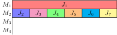
(a) Weakly recoverable optimal $S_{init}$.

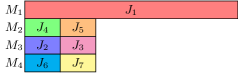
(b) Efficiently recoverable LexOpt $S_{init}$.

Figure 3: Illustration of the benefit obtained by LexOpt schedules.

Before proving Theorem 4, we state Lemma 4 which relates the optimal makespan of two instances with a different number of machines and set of jobs. Denote by $C_{\max}^{*}(m,\mathcal{J})$ the optimal makespan for instance $(m,\mathcal{J})$. Lemma 4 highlights the importance of a LexOpt schedule: consider a LexOpt schedule $S^{*}$ for $(m,\mathcal{J})$ and an arbitrary subset $\mathcal{M}^{\prime}\subseteq\mathcal{M}$ of $m-1$ machines, i.e. $\mathcal{M}^{\prime}=\mathcal{M}\setminus\{M_{\ell}\}$. Also, let $\mathcal{J^{\prime}}$ be the subset of jobs assigned to the machines in $\mathcal{M}^{\prime}$ by $S^{*}$. Then, the subschedule of $S^{*}$ on $\mathcal{M}^{\prime}$ is optimal for $(m-1,\mathcal{J}^{\prime})$.

Lemma 4

Consider a makespan problem instance $(m,\mathcal{J})$ and let $S$ be LexOpt schedule. Given an arbitrary machine $M_{\ell}\in\mathcal{M}$, denote by $\mathcal{J}^{\prime}$ the subset of all jobs assigned to the machines in $\mathcal{M}\setminus\{M_{\ell}\}$ by $S$. Then, it holds that:

1. $\max_{M_{i}\in\mathcal{M}\setminus\{M_{\ell}\}}\{C_{i}(S)\}=C_{\max}^{*}(m-1,\mathcal{J}^{\prime})$, and

2. $C_{\max}^{*}(m-1,\mathcal{J})\leq 2\cdot C_{\max}^{*}(m,\mathcal{J})$.

Theorem 4

For the makespan recovery problem with a single perturbation, Algorithm 3 achieves a tight price of robustness equal to 2, if $S_{init}$ is LexOpt.

Proof:
The sequel proves the theorem in the case of a job reduction. For other perturbations described in Section 2, the proof is presented in the supplementary material. The supplementary material also shows that the obtained price of robustness is tight for every perturbation that we consider.

Consider a LexOpt schedule $S_{init}$ for instance $I_{init}$ and suppose that the processing time of job $J_{j}$ decreases by $\delta\in(0,p_{j}]$, i.e. $p_{j}\leftarrow p_{j}-\delta$. Cancelling job $J_{j}\in\mathcal{J}$ is equivalent to reducing $p_{j}$ to zero. Suppose that machine $M_{\ell}$ executes $J_{j}$ in $S_{init}$. W.l.o.g., job $J_{j}$ completes last in $M_{\ell}$. Algorithm 3 returns the recovered schedule $S_{rec}$ which keeps the job assignments in $S_{init}$, but decreases $p_{j}$ and $C_{\ell}(S_{init})$ by $\delta$. Let $S_{new}$ be an optimal schedule for the perturbed instance $I_{new}$. We distinguish two cases depending on whether $M_{\ell}$ completes last in $S_{rec}$, or not.

First, suppose $C_{\ell}(S_{rec})<C_{\max}(S_{rec})$ and let $\mathcal{J}^{\prime}\subseteq\mathcal{J}$ be the subset of jobs executed by the machines in $\mathcal{M}\setminus\{M_{\ell}\}$. Then,

$$C_{\max}(S_{rec})=\ C_{\max}^{*}(m-1,\mathcal{J}^{\prime}) [\text{Lemma \ref{Lemma:Single_Lexicographic_Optimal_Substructure}.1}],$$

$$\leq\ C_{\max}^{*}(m-1,\mathcal{J}\setminus\{J_{j}\}) [\mathcal{J}^{\prime}\subseteq\mathcal{J}\setminus\{J_{j}\}],$$

$$\leq\ 2\cdot C_{\max}^{*}(m,\mathcal{J}\setminus\{J_{j}\}) [\text{Lemma \ref{Lemma:Single_Lexicographic_Optimal_Substructure}.2}],$$

$$\leq\ 2\cdot C_{\max}(S_{new}) [\text{Definition}].$$

Subsequently, consider that $C_{\ell}(S_{rec})=C_{\max}(S_{rec})$, i.e. $C_{\max}(S_{rec})=C_{\max}(S_{init})-\delta$. We claim that $S_{rec}$ is optimal for $I_{new}$. Assume for contradiction that an optimal schedule $S_{new}$ for $I_{new}$ satisfies $C_{\max}(S_{new})<C_{\max}(S_{init})-\delta$. By adding $\delta$ extra units of time on job $J_{j}$, we derive a feasible schedule $\widetilde{S}$ for $I_{init}$ from $S_{new}$, such that $C_{\max}(\widetilde{S})<C_{\max}(S_{init})$. This contradicts the optimality of $S_{init}$ for $I_{init}$.  

4.3 Multiple Perturbations

Two-stage robust optimization can be viewed as a two-player game where (i) we solve an initial instance, (ii) a malicious adversary generates perturbations, and (iii) we transform the initial solution into an efficient solution for a new instance. Adversarial strategies with multiple perturbations can render the initial solution weakly reoptimizable. But LexOpt can manage a bounded degree of uncertainty. For this case, we show that Algorithm 3 produces solutions with a positive performance guarantee parameterized by the uncertainty set size. Definition 3 describes our uncertainty set $\mathcal{U}(f,k,\delta)$ with three parameters: (i) the factor $f$ indicating the boundary between stable and unstable job perturbations, (ii) the number $k$ of unstable jobs, and (iii) the number $\delta$ of surplus machines. We assume that the number $k$ of unstable jobs is bounded by the number of machines $m$, i.e. $k<m$.

Definition 3

For a makespan problem instance $(m,\mathcal{J})$ with processing times $p_{1}$, $\ldots$, $p_{n}$, the uncertainty set $\mathcal{U}(f,k,\delta)$ contains every instance $(\hat{m},\hat{\mathcal{J}})$ with processing times $\hat{p}_{1},\ldots,\hat{p}_{n}$ satisfying the following properties:

• Stability/instability boundary. $\hat{\mathcal{J}}$ can be partitioned into the set $\hat{\mathcal{J}}^{s}$ of stable jobs and the set $\hat{\mathcal{J}}^{u}$ of unstable jobs, where $p_{j}/f\leq\hat{p}_{j}\leq p_{j}\cdot f$ $\forall$ $J_{j}\in\hat{\mathcal{J}}^{s}$.

• Bounded number of unstable jobs. $|\hat{\mathcal{J}}^{u}|\leq k$, assuming that $k<m$.

• Bounded number of surplus machines. $\max\{\hat{m}-m,0\}\leq\delta$.

Suppose $C_{\max}^{*}(m,\mathcal{J})$ is the optimal makespan for the $P||C_{\max}$ instance $(m,\mathcal{J})$. Lemma 5 (i) formalizes the optimal substructure imposed by LexOpt, (ii) bounds pairwise machine completion time differences in LexOpt schedules, (iii) quantifies the sensitivity of the optimal makespan w.r.t. the number of machines, and (iv) quantifies sensitivity of the optimal makespan w.r.t. processing times.

Lemma 5

Let $(m,\mathcal{J})$ be a makespan problem instance with a LexOpt schedule $S$.

1. If the subset $\mathcal{J}^{\prime}\subseteq\mathcal{J}$ of jobs is executed by the subset $\mathcal{M}^{\prime}\subseteq\mathcal{M}$ of machines in $S$, where $|\mathcal{M}^{\prime}|=m^{\prime}$, then the sub-schedule of $S$ on $\mathcal{M}^{\prime}$ is optimal for $(m^{\prime},\mathcal{J}^{\prime})$, i.e. $\max_{M_{i}\in\mathcal{M}^{\prime}}\{C_{i}(S)\}=C_{\max}^{*}(m^{\prime},\mathcal{J}^{\prime})$.

2. Assuming that $M_{i},M_{\ell}\in\mathcal{M}$ are two different machines such that job $J_{j}\in\mathcal{J}$ is assigned to $M_{i}$ in $S$, then $C_{\ell}(S)\geq C_{i}(S)-p_{j}$.

3. It holds that $C_{\max}^{*}(m-\ell,\mathcal{J})\leq\left(1+\left\lceil\frac{\ell}{m-\ell}\right\rceil\right)\cdot C_{\max}^{*}(m,\mathcal{J})$ $\forall$ $\ell\in\{1,\ldots,m-1\}$.

4. Let $(m,\hat{\mathcal{J}})$ be a makespan problem instance s.t. $\mathcal{J}=\hat{\mathcal{J}}$ and $\frac{1}{f}\cdot\hat{p}_{j}\leq p_{j}\leq\hat{p}_{j}$ for each $J_{j}$, where $p_{j}$ and $\hat{p}_{j}$ is the processing time of $J_{j}$ in $\mathcal{J}$ and $\hat{\mathcal{J}}$, respectively. Then, $\frac{1}{f}\cdot C_{\max}^{*}(m,\hat{\mathcal{J}})\leq C_{\max}^{*}(m,\mathcal{J})\leq C_{\max}^{*}(m,\hat{\mathcal{J}})$.

Table 1: Performance guarantees of our two-stage approach for different perturbations, parameterized by the (i) perturbation factor $f$, (ii) number $k<m$ of unstable jobs, and (iii) number $\delta$ of surplus machines. The term $\rho$ is the product of the performance guarantees obtained for Types 1-3.

Type	Perturbation type	Performance guarantee
Type 1	Job cancellations, Processing time reductions	$2f\cdot(1+\lceil\frac{k}{m-k}\rceil)$
Type 2	Processing time augmentations	$f+k$
Type 3	Machine activations	$(1+\lceil\delta/m\rceil)$
Type 4	Job arrivals, Machine failures	$\max\{2,\rho\}$

Table 1 lists performance guarantees for our two-stage approach, obtained by individually analyzing each type of perturbation. Despite distinguishing the arguments for each type of perturbation, we obtain a global price of robustness for all perturbations simultaneously by propagating the solution degradation with respect to the order of Table 1. Considering perturbations in this order is only for analysis purposes and does not restrict our uncertainty model. Theoretically, LexOpt is essential only for bounding the solution degradation due to job removals and processing time reductions. But practically, the optimal substructure imposed by LexOpt is beneficial in an integrated setting with all possible perturbations. Section 5 complements the theoretical analysis with numerical experiments highlighting the significance of LexOpt in the recovered solution quality. Theorem 5 quantifies the price of robustness for our two-stage approach.

Theorem 5

For the two-stage robust makespan scheduling problem with $\mathcal{U}(f,k,\delta)$ uncertainty and $k<m$, our LexOpt-based approach achieves a price of robustness:

$$2f\cdot\left(1+\left\lceil\frac{k}{m-k}\right\rceil\right)\cdot(f+k)\cdot\left(1+\left\lceil\frac{\delta}{m}\right\rceil\right).$$

Proof:
Next, we analyze the recovered solution after job cancellations and processing time reductions (Type 1). The supplementary material completes the theorem’s proof for the other perturbations (Types 2-4). Further, the supplementary material shows that the obtained price of robustness is asymptotically tight.

Processing time reductions are only recovered using binding decisions. A job cancellation is equivalent to reducing the processing time to zero. Given the recovered schedule $S_{rec}$, we partition the machines $\mathcal{M}$ into the sets $\mathcal{M}^{s}$ of stable machines, which are not assigned unstable jobs, and $\mathcal{M}^{u}$ of unstable machines, which are assigned unstable jobs. That is, $C_{i}(S_{rec})\geq\frac{1}{f}\cdot C_{i}(S_{init})$, for $M_{i}\in\mathcal{M}^{s}$, and $m^{s}=|\mathcal{M}^{s}|\geq m-k$. Also, $\mathcal{M}^{u}=\mathcal{M}\setminus\mathcal{M}^{s}$ and $m^{u}=|\mathcal{M}^{u}|\leq k$. Machine $M_{i}\in\mathcal{M}$ is critical, if it completes last in schedule $S_{rec}$, i.e. $C_{i}(S_{rec})=C_{\max}(S_{rec})$. We distinguish two cases based on whether $\mathcal{M}^{s}$ contains a critical machine, or not.

Case 1: $\mathcal{M}^{s}$ contains a critical machine

Let $\mathcal{J}_{new}^{s}\subseteq\mathcal{J}$ be the jobs assigned to machines $\mathcal{M}^{s}$ by $S_{rec}$. Each job in $\mathcal{J}_{new}^{s}$ is perturbed by a factor of at most $f$. Let $\mathcal{J}_{init}^{s}$ denote the same jobs before uncertainty realization. Jobs in $\mathcal{J}_{init}^{s}$ are executed on $\mathcal{M}^{s}$ in $S_{init}$ and appear in $\mathcal{J}_{new}^{s}$ with smaller processing times. Then,

$$C_{\max}(S_{rec}) =\max_{M_{i}\in\mathcal{M}^{s}}\{C_{i}(S_{rec})\} \mathcal{M}^{s}$$ [ contains a critical machine],

$$\leq\max_{M_{i}\in\mathcal{M}^{s}}\{C_{i}(S_{init})\}$$ [Processing time reduction],

$$=C_{\max}^{*}(m^{s},\mathcal{J}_{init}^{s})$$ [Lemma 5.1],

$$\leq f\cdot C_{\max}^{*}(m^{s},\mathcal{J}_{new}^{s})$$ [Lemma 5.4],

$$\leq f\cdot C_{\max}^{*}(m^{s},\mathcal{J}_{new}) \mathcal{J}_{new}^{s}\subseteq\mathcal{J}_{new}$$ [],

$$=f\cdot C_{\max}^{*}(m-m^{u},\mathcal{J}_{new}) m^{s}=m-m^{u}$$ [],

$$\leq f\cdot\left(1+\left\lceil\frac{m^{u}}{m-m^{u}}\right\rceil\right)\cdot C_{\max}^{*}(m,\mathcal{J}_{new})$$ [Lemma 5.3],

$$\leq f\cdot\left(1+\left\lceil\frac{k}{m-k}\right\rceil\right)\cdot C_{\max}(S_{new}). m^{u}\leq k$$ []

Case 2: Only $\mathcal{M}^{u}$ contains critical machines

Consider an unstable critical machine $M_{i}\in\mathcal{M}^{u}$ in $S_{rec}$, i.e. $C_{\max}(S_{rec})=C_{i}(S_{rec})$. If only one job is assigned to $M_{i}$, then schedule $S_{rec}$ is optimal. Now, assume that at least two jobs are assigned to $M_{i}$ in $S_{rec}$ . Since processing times are only reduced, $C_{i}(S_{rec})\leq C_{i}(S_{init})$. Because $k<m$, there exists a machine $M_{\ell}\in\mathcal{M}^{s}$. Furthermore, since $S_{init}$ is LexOpt, Lemma 5.2 ensures that $C_{\ell}(S_{init})\geq C_{i}(S_{init})-p_{j}$, for each $J_{j}\in\mathcal{J}$ assigned to $M_{i}$ by $S_{init}$. As $S_{init}$ contains at least two jobs, there exists a job $J_{j}$ assigned to $M_{i}$ by $S_{init}$ such that $p_{j}\leq\frac{1}{2}\cdot C_{i}(S_{init})$. Hence, $C_{i}(S_{init})\leq 2\cdot C_{\ell}(S_{init})$. We conclude that $C_{\max}(S_{rec})\leq 2\cdot C_{\ell}(S_{init})$. Because $M_{\ell}\in\mathcal{M}^{s}$, similarly to Case 1, we get:

$$C_{\max}(S_{rec})\leq 2f\cdot\left(1+\left\lceil\frac{k}{m-k}\right\rceil\right)\cdot C_{\max}(S_{new}).$$

 

5 Numerical Results

Section 5.1 describes our system specifications and the generation of benchmark $P||C_{\max}$ instances. Section 5.2 evaluates the LexOpt branch-and-bound algorithm. Section 5.3 presents the generation of perturbed instances, i.e. the effect of uncertainty realization. Section 5.4 evaluates the price of robustness of our two-stage robust scheduling approach.

5.1 System Specification and Benchmark Instances

We ran all computations on an Intel Core i7-4790 CPU 3.60GHz, 15.6 GB RAM machine running Ubuntu 14.04 64-bit. Using Python 2.7.6 and Pyomo 4.4.1, we solve MILP models with CPLEX 12.6.3 and Gurobi 6.5.2. The source code and test cases are available on GitHub [34]. We have randomly generated $P||C_{\max}$ instances. Well-formed instances admit an optimal schedule close to a perfect solution where all machine completion times are equal, i.e. $C_{i}=C_{i^{\prime}}$ for $M_{i},M_{i^{\prime}}\in\mathcal{M}$. Degenerate instances have a less-balanced optimal schedule. This section investigates well-formed instances and we complete the analysis with degenerate instances in the supplementary material.

Well-formed instances depend on 3 parameters: (i) the number $m$ of machines, (ii) the number $n$ of jobs, and (iii) a processing time seed $q$. Using the parameter values in Table 2, we generated moderate, intermediate and hard well-formed instances. For each combination of $m$, $n$ and $q$, we generate 3 instances based on 3 different distributions of processing times: uniform distribution $p_{j}\sim\mathcal{U}(\{1,\ldots,q\})$, normal distribution $p_{j}\sim\mathcal{N}(q,q/3)$ and a symmetric of normal distribution s.t. $p\sim\mathcal{N}(q,q/3)$ and $p_{j}=q-p$ if $p\in[0,q]$, or $p_{j}=2q-(p-q)$ if $p_{j}\in(q,2q]$. Each processing time is rounded to the nearest integer. Further, (symmetric) normal processing times outside $[0,2q]$ are rounded to the nearest of $0$ and $2q$.

Table 2: Well-formed Instances

Instances	$\mathbf{m}$	$\mathbf{n}$	$\mathbf{q}$
Moderate	$3,4,5,6$	$20,30,40,50$	$100,1000$
Intermediate	$10,12,14,16$	$100,200,300,400$	$10000,100000$
Hard	$10,15,20,25$	$200,300,400,500$	$10000,100000$

5.2 LexOpt Branch-and-Bound Algorithm Evaluation

This section numerically evaluates our branch-and-bound algorithm. We complement our evaluation with the sequential, highest-rank objective, and weighting methods adapted to LexOpt scheduling. Our termination criteria for each MILP solving is: (i) $10^{3}$ CPU seconds time limit, and (ii) $10^{-4}$ relative error tolerance, where the relative gap $(Ub-Lb)/Ub$ is computed using the best-found incumbent $Ub$ and the lower bound $Lb$.

The sequential method solves $m$ MILP instances with repeated CPLEX calls, using the CPLEX reoptimize feature in each call to exploit information obtained from previous calls. If $10^{3}$ CPU seconds in total elapse, then the method terminates when the ongoing MILP run is completed. The highest-rank objective method solves the LexOpt scheduling problem using the CPLEX solution pool feature. Initially, the standard MILP model for $P||C_{\max}$ is solved. Next, the tree exploration goes on and populates a pool with 2000 solutions. The weighting method computes a schedule $S$ of minimal weighted value $W(S)=\sum_{i=1}^{m}B^{m-i}\cdot C_{i}(S)$. We set $B=2$ and solve the resulting MILP models with CPLEX and Gurobi.

Figure 4 plots performance profiles of LexOpt methods on well-formed instances in order to compare running times and computed solutions [20]. The sequential and weighting methods perform similarly in terms of running time and number of solved instances. But, the sequential method produces worse feasible solutions since lower-ranked objectives are not optimized in the case of a timeout. The highest-rank objective method has worse running times than the sequential and weighting methods on moderate instances, because populating the solution pool is a significant part of the overall running time. However, the highest-rank objective method attains significantly better running times than the sequential and weighting methods on intermediate and hard test cases, because populating the solution pool is a small fraction of the overall running time. The highest-rank objective method does not prove lexicographic optimality as it only generates 2000 candidate solutions. Nonetheless, it produces the best heuristic results for most test cases.

Figure 4 shows that our branch-and-bound algorithm proves global optimality faster than the other methods when it converges, i.e. when it does not timeout. Note that the branch-and-bound algorithm converges for $>60\%$ of the moderate test cases and $>30\%$ of the intermediate and hard instances. For intermediate and hard instances, the branch-and-bound algorithm consistently produces good heuristic solutions, i.e. better solutions than the sequential and weighting methods.

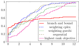
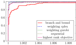
(a) Moderate instances: time (s) on $\log_{2}$ scale (left), upper bounds on $[1,1.009]$ (right).

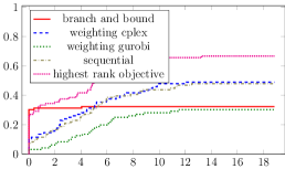
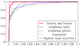
(b) Intermediate instances: time (s) on $\log_{2}$ scale (left), upper bounds on $[1,1.1]$ (right).

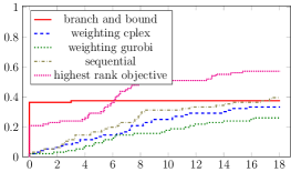
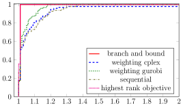
(c) Hard instances: time (s) on $\log_{2}$ scale (left), upper bounds on $[1,2]$ (right).

Figure 4: Performance profiles for the well-formed test set with $10^{3}$ s timeout.

5.3 Generation of Perturbed Instances

Recall that an instance of the makespan recovery problem is specified by: (i) an initial makespan problem instance $I_{init}$, (ii) an initial solution $S_{init}$ to $I_{init}$, and (iii) a perturbed instance $I_{new}$. We generate the initial $P||C_{\max}$ instances according to Section 5.1. For each instance $I_{init}$, we generate a set $\mathcal{S}(I_{init})$ of 50 schedules using the CPLEX solution pool feature. In general, two different schedules $S_{1},S_{2}\in\mathcal{S}(I_{init})$ have weighted values $W(S_{1})\neq W(S_{2})$, where $W(S)=\sum_{i=1}^{m}B^{m-i}\cdot C_{i}(S)$. For each makespan problem instance $I_{init}$, we construct a perturbed instance $I_{new}$ by generating random disturbances. A job disturbance is (i) a new job arrival, (ii) a job cancellation, (iii) a processing time augmentation, or (iv) a processing time reduction. A machine disturbance is (i) a new machine activation, or (ii) a machine failure. We randomly generate $d_{n}=\lceil 0.2\cdot n\rceil$ job disturbances and $d_{m}=\lceil 0.2\cdot m\rceil$ machine perturbations. The type of each job disturbance is chosen uniformly at random among the four options (i) - (iv). A new job $J_{j}\in\hat{\mathcal{J}}$ has processing time $\hat{p}_{j}\sim\mathcal{U}(\{1,\ldots,q\})$, using the parameter $q$ that produced the original instance $I_{init}$. A job cancellation deletes an existing job chosen uniformly at random. To increase or decrease the processing time of job $J_{j}\in\mathcal{J}$, we randomly select $\hat{p}_{j}\sim\mathcal{U}(\{p_{j}+1,\ldots,2\cdot q\})$ or $\hat{p}_{j}\sim\mathcal{U}(\{1,2,\ldots p_{j}-1\})$, respectively. The type of a machine disturbance is chosen uniformly at random among options (i)-(ii). A new machine activation increases the number of available machines by one. A machine cancellation deletes an existing machine chosen uniformly at random.

5.4 Two-Stage Robust Scheduling Evaluation

In the two-stage robust makespan scheduling problem, solution $S_{init}$ is transformed to a feasible solution $S_{rec}$ for instance $I_{new}$. Figure 5 correlates the makespan of $S_{rec}$ with the closeness of $S_{init}$ to LexOpt. We quantify the closeness of $S_{init}$ to LexOpt using the weighted value $W(S_{init})=\sum_{i=1}^{m}B^{m-i}\cdot C_{i}(S_{init})$. The closest to LexOpt the schedule $S_{init}$ is, the lowest the value $W(S_{init})$ we get. For each instance $I_{init}$, we recover every solution $S_{init}\in\mathcal{S}(I_{init})$ by applying our binding and flexible recovery strategies from Section 4.1. For the flexible recovery strategy, we set $g=0.1n$, i.e. at most 10% of the binding decisions can be modified. Suppose that the normalized weighted value of an initial solution $S_{init}\in\mathcal{S}(I_{init})$ is $W^{N}(S_{init})=\frac{W(S_{init})}{W^{*}(I_{init})}$, where $W^{*}(I_{init})$ is the best weighted value in the CPLEX solution pool for instance $I_{init}$. Similarly, assume that the normalized makespan of $S_{rec}$ equal to $C^{N}(S_{rec})=\frac{C_{\max}(S_{rec})}{C_{\max}^{*}(I_{new})}$, where $C_{\max}^{*}(I_{new})$ is the makespan of the best recovered schedule for instance $I_{new}$. Figure 5(a) shows that the makespan of solutions obtained with our binding recovery strategy tends to improve as the weighted value of the initial solution decreases. Figure 5(b) verifies this trend for the flexible recovery strategy. These results highlight the importance of LexOpt towards efficient two-stage robust scheduling. Our findings also motivate scheduling under uncertainty where the planning and recovery stages are investigated together.

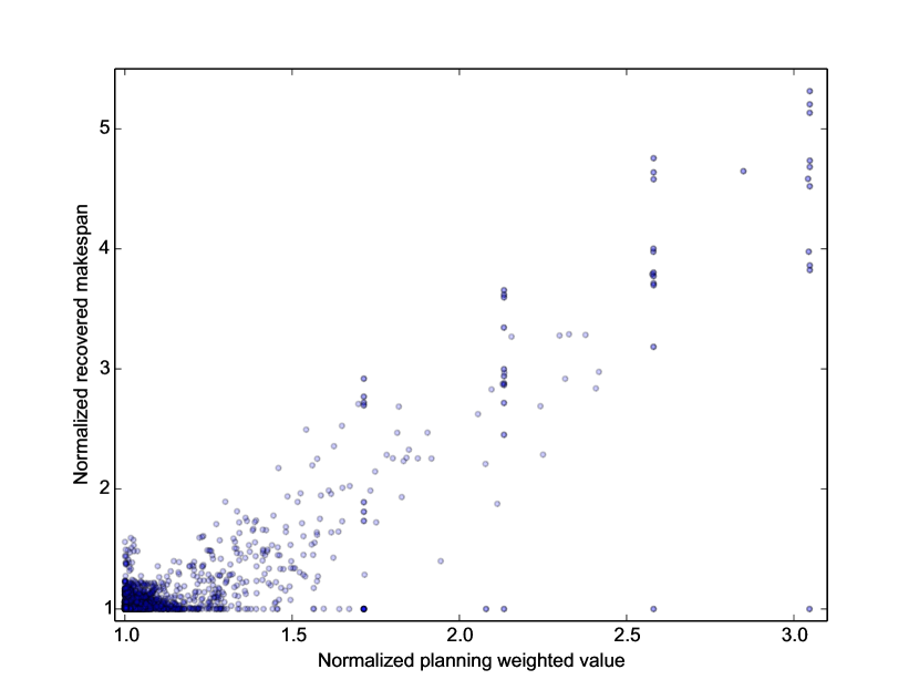
(a) Binding Recovery

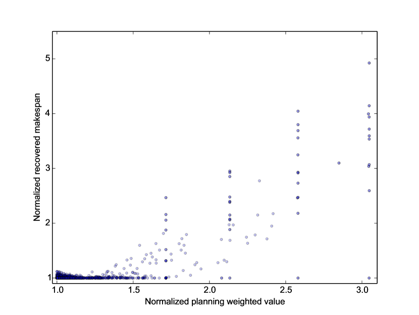
(b) Flexible Recovery

Figure 5: Well-formed instances scatter plots illustrating the recovered solution makespan with respect to the initial solution weighted value.

6 Conclusion

Practical scheduling applications frequently require an initial, nominal schedule which is recovered after uncertainty realization. But significantly modifying the nominal schedule might not be desirable in domains such as distributed computing [57] and timetabling [46]. To this end, we use exact LexOpt scheduling for planning and approximate rescheduling for adaptability [2, 7, 17, 49].

We provide new insights on the combinatorial structure of robust scheduling. LexOpt handles highly-symmetric mixed-integer optimization problems [3, 23, 22, 47], but our results also highlight LexOpt benefits on scheduling under uncertainty. By exploiting optimal substructure imposed by LexOpt, we propose a two-stage robust makespan scheduling approach whose performance is substantiated with a price of robustness characterization. Numerical results with randomly generated instances demonstrate that the closest to LexOpt the initial solution is, the better the recovered solution quality we get. Beyond scheduling, extensions to uncertain min-max partitioning problems, e.g. facility location and network design, with generalized cost functions are possible [55].

Faced with the lack of strong lower bounding techniques for LexOpt scheduling, we develop a new branch-and-bound algorithm, based on vectorial bounds. The algorithm (i) avoids iterative MILP solving of sequential methods, (ii) bypasses precision issues of weighting methods, and (iii) reduces the symmetry of highest-rank objective methods. This approach is broadly relevant to LexOpt.

Acknowledgments
We gratefully acknowledge support from Engineering & Physical Sciences Research Council Research (EPSRC) [EP/M028240/1] and a Fellowship to RM [EP/P016871/1].

Contents

This document contains omitted parts of the manuscript Exact Lexicographic Scheduling and Approximate Rescheduling. The document is a companion to the original manuscript for readers interested in complementary technicalities which have been omitted to better convey our main message, i.e. the importance of LexOpt in scheduling under uncertainty and relevant challenges. These technicalities are essential for the completeness of the presented study. The manuscript itself and this supplementary document cover the topics in a similar order.

Appendix A provides omitted parts required for designing, analyzing, and evaluating the exact LexOpt methods. Appendix B shows that the makespan recovery problem is $\mathcal{NP}$-hard. Appendices C and D complete the robustness analysis of our two-stage approach in the case of a single and multiple perturbations, respectively. Appendix E presents a more flexible recovery strategy. Appendix F completes our numerical evaluation with degenerate instances. Finally, Appendix G provides a table with the notation used in both documents.

Appendix A Exact LexOpt Methods

Section A.1 proves valid inequalities and Section A.2 adapts the sequential, weighting, and highest-rank objective methods for the LexOpt scheduling problem. Section A.3 provides a pseudo-code, Section A.4 describes a primal heuristic, Section A.5 provides correctness proofs for the vectorial bounds and Section A.6 states a correctness proof for our branch-and-bound algorithm.

A.1 LexOpt Scheduling Reformulation Lemma

Lemma 1

In an optimal solution to the LexOpt scheduling problem:

1. $C_{i}\geq C_{i+1}$, for $i=1,\ldots,m-1$,

2. $i\cdot C_{i}+\left[\sum_{q=i+1}^{m}C_{q}\right]\leq\sum_{j=1}^{n}p_{j}\leq\left[\sum_{q=1}^{i-1}C_{q}\right]+(m-i+1)\cdot C_{i}$, $\forall$ $i=1,\ldots,m$.

Proof:
In any feasible schedule, the machines can be renumbered so as to satisfy the first property. For the second property, observe that $\sum_{i=1}^{m}C_{i}=\sum_{j=1}^{n}p_{j}$. Since $C_{i}\geq\ldots\geq C_{m}$, we get that $\sum_{q=1}^{i-1}C_{q}+(m-i+1)\cdot C_{i}\geq\sum_{j=1}^{n}p_{j}$. Similarly, given that $C_{1}\geq\ldots\geq C_{i}$, we conclude that $i\cdot C_{i}+\sum_{q=i+1}^{m}C_{q}\leq\sum_{j=1}^{n}p_{j}$.  

A.2 State-of-the-Art LexOpt Methods

Sequential Method

This method (Algorithm 4) iteratively minimizes the objective functions $C_{1},\ldots,C_{n}$ w.r.t. to their priority order, over the set $\mathcal{S}$ of feasible schedules [16, 19]. Let $v_{i}^{*}$ be the value of $C_{i}$ in a LexOpt solution. The $i$-th iteration computes $v_{i}^{*}$ by solving MILP (1) with the extra constraint that the first $(i-1)$ objectives should be respectively equal to $v_{1}^{*},\dots,v_{i-1}^{*}$. Warm-starting iteration $i$ with the solution at iteration $(i-1)$ improves the efficiency of the method.

Algorithm 4 Sequential Method

1:$v_{1}^{*}=\min\{C_{1}:(\vec{x},\vec{C})\in\mathcal{S}\}$.

2:for $i=2,\ldots,m$ do

3:     $v_{i}^{*}=\min\{C_{i}:x\in\mathcal{S},C_{1}=v_{1}^{*},\ldots,C_{i\text{-}1}=v_{i\text{-}1}^{*}\}$

4:Return the solution computed in the last iteration.

Weighting Method

This method (Algorithm 5) minimizes a weighted sum $\sum_{i=1}^{m}w_{i}\cdot C_{i}$ of the objectives $C_{1},\ldots,C_{n}$ [51]. Typically, $w_{i}=B^{m-i}$ for $i=1,2,\ldots,m$, where the big-M parameter $B>1$ is a sufficiently large constant [52]. Note that the highest-rank objectives are associated with the largest weights. Further, this weighted sum can measure the distance of any solution from the LexOpt solution. For our numerical results, we set $B=2$.

Algorithm 5 Weighting Method

1:Select big-M parameter $B=2$.

2:for $i=2,\ldots,m$ do

3:     Set machine weight $w_{i}=B^{m-i}$.

4:Solve $\min\{\sum_{i=1}^{m}w_{i}\cdot C_{i}:(\vec{x},\vec{C})\in\mathcal{S}\}$.

Highest-Rank Objective Method

This method (Algorithm 6) computes the pool $\mathcal{P}$ of all optimal solutions for the mono-objective problem $v_{1}^{*}=\min\{C_{1}:(\vec{x},\vec{C})\in\mathcal{S}\}$ of minimizing the highest-rank objective function $C_{1}$, i.e. the makespan, and returns the lexicographically smallest solution $\text{lex}\min\{\vec{C}(S):\;S\in\mathcal{P}\}$ in $\mathcal{P}$ [44]. A very large solution pool can be efficiently approximated with a smaller set of solutions using the CPLEX solution pool feature. In LexOpt, maintaining a single solution in the pool is sufficient, if the current solution is always replaced by a lexicographically smaller solution. A simple greedy lexicographic comparison algorithm checks when such an update is essential.

Algorithm 6 Highest-Rank Objective Method

1:Solve $v_{1}^{*}=\min\{C_{1}:(\vec{x},\vec{C})\in\mathcal{S}\}$.

2:Compute the solution pool $\mathcal{P}=\{(\vec{x},\vec{C})\in\mathcal{S}:C_{1}=v_{1}^{*}\}$.

3:Return $\text{lex}\min\{\vec{C}:(\vec{x},\vec{C})\in\mathcal{P}\}$.

A.3 Branch-and-Bound Algorithm Pseudocode

Algorithm 7 LexOpt Branch-and-Bound Algorithm using Vectorial Bounds

1:$Q$: empty stack

2:$r$: root node

3:$\text{push}(Q,r)$

4:$I=\{+\infty\}^{m}$

5:while $Q\neq\emptyset$ do

6:     $u=\text{top}(Q)$

7:     for $v\in\text{children}(u)$ do

8:         if $v$ is leaf then

9:              $S$: schedule of $v$

10:              $I=\text{lex}\min\{I,S\}$

11:         else

12:              $S$: heuristic schedule computed via LPT

13:              $I=\text{lex}\min\{I,S\}$

14:              $\vec{L}$: vectorial lower bound of node $v$

15:              if $\vec{L}\leq_{\mathrm{lex}}\vec{C}(I)$ then

16:                  $\text{push}(Q,v)$                             

A.4 Longest Processing Time First Heuristic

The primal heuristic applied in each node $v$ of the branch-and-bound tree is Longest Processing Time First (LPT) (Algorithm 8). LPT keeps the assignment of jobs $J_{1},\ldots,J_{\ell}$, where $\ell$ is the level of node $v$, and greedily schedules jobs $J_{\ell+1},\ldots,J_{n}$ with the order $p_{\ell+1}\geq\ldots\geq p_{n}$. In each step, LPT assigns the next job to the least-loaded machine, i.e. makes the lexicographically best decision.

Algorithm 8 Longest Processing Time First (LPT) at level $\ell$

1:$\vec{t}$: Initial machine completion times

2:for $j=(\ell+1),\ldots,n$ do

3:     $i=\arg\min_{M_{q}\in\mathcal{M}}\{t_{q}\}$

4:     $C_{i}\leftarrow t_{i}+p_{j}$

5:Sort the machines so that $C_{1}\geq\ldots\geq C_{m}$.

A.5 Correctness of Vectorial Bounds

This section proves Lemmas 2-3 and, thus, shows that Algorithms 1-2 correctly compute vectorial bounds.

(a) Partial schedule associated with node $v$.

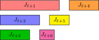
(b) Remaining jobs.

Figure 6: Computing vectorial lower bound component $L_{i}$ at node $v$ in the $\ell$-th search tree level, by scheduling jobs $J_{\ell+1},\ldots,J_{n}$ in the partial schedule of $v$. Jobs $J_{\ell+1},\ldots,J_{h}$ are rejected in the intervals $[t_{q},U_{q}]$, for $q=1,\ldots,i-1$. $L_{i}$ is computed by fractionally scheduling jobs $J_{h+1},\ldots,J_{m}$ on machines $M_{i},\ldots,M_{m}$ and lower bounding the completion time of machine $M_{i}$.

Lemma 2

Consider a node $v$ of the search tree and a machine index $i\in\{1,\ldots,m\}$. Algorithm 1 produces a value $L_{i}\leq C_{i}(S)$ for each feasible schedule $S\in\mathcal{S}(v)$ below $v$ such that $C_{q}(S)\leq U_{q}$, $\forall$ $q=1,\ldots,i-1$.

Proof:
Schedule $S$ and pseudo-schedule $\widetilde{S}$ (of Algorithm 1) assign jobs $J_{1},\ldots,J_{\ell}$ to the same machines and the vector $\vec{t}=(t_{1},\ldots,t_{m})$ specifies machine completion times w.r.t. these jobs. All remaining jobs $\mathcal{R}=\{J_{\ell+1},\ldots,J_{n}\}$ are scheduled differently in $\widetilde{S}$ and $S$. In $\widetilde{S}$, the jobs in $\mathcal{\widetilde{R}}=\{J_{\ell+1},\ldots,J_{h}\}$ are fractionally assigned to machines $M_{1},\ldots,M_{i-1}$ and the jobs in $\mathcal{R}\setminus\widetilde{\mathcal{R}}=\{J_{h+1},\ldots,J_{n}\}$ to $M_{i},\ldots,M_{m}$. Denote by $\mathcal{R}^{\prime}\subseteq\mathcal{R}$ the corresponding subset of jobs assigned to machines $M_{1},\ldots,M_{i-1}$, in $S$. That is, the jobs in $\mathcal{R}\setminus\mathcal{R}^{\prime}$ are assigned to $M_{i},\ldots,M_{m}$ in $S$.

Observe that $\sum_{J_{j}\in\mathcal{R}^{\prime}}p_{j}=\sum_{q=1}^{i-1}\left(C_{q}(S)-t_{q}\right)\leq\sum_{q=1}^{i-1}\left(U_{q}-t_{q}\right)$ $\leq\sum_{J_{j}\in\widetilde{\mathcal{R}}}p_{j}$, where the first equality holds by definition, the first inequality by the assumption $C_{q}(S)\leq U_{q}$, for $q=1,\ldots,(i-1)$, and the second inequality because Algorithm 1 fits machines $M_{1},\ldots,M_{i-1}$ at least up to their respective upper bounds. Moreover, we have that $\max_{J_{j}\in\mathcal{R}\setminus\mathcal{R}^{\prime}}\{p_{j}\}\geq\max_{J_{j}\in\mathcal{R}\setminus\widetilde{\mathcal{R}}}\{p_{j}\}=p_{h+1}$. Otherwise, $\max_{J_{j}\in\mathcal{R}\setminus\mathcal{R}^{\prime}}\{p_{j}\}<p_{h+1}$, which implies that $\mathcal{R}^{\prime}$ contains all jobs $J_{\ell+1},\ldots,J_{h+1}$. Hence, $\sum_{J_{j}\in\mathcal{R}^{\prime}}p_{j}\geq\sum_{j=\ell+1}^{h+1}p_{j}>\sum_{J_{j}\in\widetilde{\mathcal{R}}}p_{j}$, i.e. a contradiction.

Since $S$ assigns a job of processing time $\max_{J_{j}\in\mathcal{R}\setminus\mathcal{R}^{\prime}}\{p_{j}\}\geq p_{h+1}$ to a machine in $M_{i},\ldots,M_{m}$, $C_{i}(S)\geq\min_{i\leq q\leq m}\{t_{q}\}+\max_{J_{j}\in\mathcal{R}\setminus\mathcal{R}^{\prime}}\{p_{j}\}\geq\min_{i\leq q\leq m}\{t_{i}\}+p_{h+1}$. Clearly, $C_{i}(S)\geq\max_{i\leq q\leq m}\{t_{i}\}$. Further, using a standard packing argument and the fact that $\sum_{J_{j}\in\mathcal{R}\setminus\mathcal{R}^{\prime}}p_{j}\geq\sum_{J_{j}\in\mathcal{R}\setminus\widetilde{\mathcal{R}}}p_{j}$, if the quantity $\Lambda=\sum_{j=h+1}^{n}p_{j}-\sum_{q=i}^{m}(\tau-t_{q})$ is positive, where $\tau=\max_{i\leq q\leq m}\{t_{q}\}$, then $C_{i}(S)\geq\max_{i\leq q\leq m}\{t_{q}\}+\frac{\Lambda}{m-i+1}$. We conclude that $L_{i}\leq C_{i}(S)$.  

Lemma 3

Consider a node $v$ of the search tree and a machine index $i\in\{1,\ldots,m\}$. Algorithm 2 produces a value $U_{i}\geq C_{i}(S)$ for each feasible schedule $S\in\mathcal{S}(v)$ below $v$ such that $C_{q}(S)\geq L_{q}$, $\forall$ $q=1,\ldots,i-1$.

Proof:
Recall that jobs $J_{1},\ldots,J_{\ell}$ are identically assigned in schedule $S$ and pseudo-schedule $\tilde{S}$ of Algorithm 2. Moreover, a vector $\vec{t}=(t_{1},\ldots,t_{m})$ specifies the machine completion times of $S$ and $\tilde{S}$ w.r.t. these jobs. Let $\mathcal{R}=\{J_{\ell+1},\ldots,J_{n}\}$ be the set of remaining jobs. Denote by $\widetilde{\mathcal{R}}=\{J_{\ell+1},\ldots,J_{h}\}\subseteq\mathcal{R}$ and $\mathcal{R}^{\prime}\subseteq\mathcal{R}$ the subset of jobs assigned to machines $M_{i},\ldots,M_{m}$ in $\widetilde{S}$ and $S$, respectively. By arguing similarly to the proof of Lemma 2, $\sum_{J_{j}\in\mathcal{R}\setminus\widetilde{\mathcal{R}}}p_{j}\geq\sum_{J_{j}\in\mathcal{R}\setminus\mathcal{R}^{\prime}}p_{j}$. In addition, $\max_{J_{j}\in\mathcal{R}\setminus\widetilde{\mathcal{R}}}\{p_{j}\}\geq\max_{J_{j}\in\mathcal{R}\setminus\mathcal{R}^{\prime}}\{p_{j}\}$.

The total load of jobs $J_{\ell+1},\ldots,J_{n}$ assigned to machines $M_{i},\ldots,M_{m}$ in $S$ is clearly $\sum_{J_{j}\in\mathcal{R}\setminus\mathcal{R^{\prime}}}p_{j}\leq\lambda=\sum_{j=\ell+1}^{n}p_{j}-\sum_{q=1}^{i-1}(L_{q}-t_{q})$. To compute $U_{i}$, Algorithm 2 assigns part of $\lambda$ fractionally and uniformly to the least loaded machines among $M_{i},\ldots,M_{m}$. In particular, it sorts these machines so that $t_{i}\leq\ldots\leq t_{m}$ and assigns $\lambda$ units of processing time to machines $M_{i},\ldots,M_{\mu}$ so that they end up having the same completion time $\tau=\frac{1}{\mu-i+1}\left(\sum_{q=1}^{\mu}t_{q}+\lambda\right)$. Using a simple packing argument and the fact that $\max_{J_{j}\in\mathcal{R}}\{p_{j}\}=p_{\ell}$, we get $C_{i}(S)\leq\max\{\tau+p_{\ell},t_{m}\}$.  

A.6 Optimality of Branch-and-Bound Algorithm

Theorem 1

The branch-and-bound method computes a LexOpt solution.

Proof:
Consider a tree node $v$. Let $\vec{L}=(L_{1},\ldots,L_{m})$ and $I$ be the computed vectorial lower bound and the incumbent, when branch-and-bound Algorithm 7 explores $v$. We show the invariant that if node $v$ is pruned, then $\vec{C}(S)\geq_{\text{lex}}\vec{C}(I)$, for every schedule $S\in\mathcal{S}(v)$. Node $v$ is pruned when $L\geq_{\text{lex}}\vec{C}(I)$, i.e. (i) $L_{1}>C_{1}(I)$, (ii) $L_{q}=C_{q}(I)$ $\forall$ $q=1,\ldots,i-1$ and $L_{i}>C_{i}(I)$, for some $i\in\{2,\ldots,m-1\}$, or (iii) $L_{i}=C_{i}(I)$ $\forall$ $i=1,\ldots,m$. In case (i), because $C_{1}(S)\geq L_{1}$, it holds that $\vec{C}(S)>_{\text{lex}}\vec{C}(I)$ $\forall$ $S\in\mathcal{S}(v)$. In case (ii), either $C_{1}(S)>L_{1}$, or $C_{1}(S)=L_{1}$ $\forall$ $S\in\mathcal{S}(v)$. Let $\mathcal{S}_{1}(v)\subseteq\mathcal{S}(v)$ be the subset of schedules satisfying $C_{1}(S)=L_{1}=C_{1}(I)$. Algorithm 2 computes $U_{1}=C_{1}(I)$. By Lemma 2, either $C_{2}(S)>L_{2}$, or $C_{2}(S)=L_{2}$, for each $S\in\mathcal{S}_{1}(v)$. Let $\mathcal{S}_{2}(v)\subseteq\mathcal{S}_{1}(v)$ be the subset of schedules with $C_{2}(S)=L_{2}$. We define similarly all sets $\mathcal{S}_{1}(v),\ldots,\mathcal{S}_{i-1}(v)$. By Lemma 2, for any schedule in $\mathcal{S}_{i-1}(v)$, it holds that $C_{q}(S)=L_{q}=C_{q}(I)$ $\forall$ $q=1,\ldots,i-1$ and $C_{i}(S)\geq L_{i}>C_{i}(I)$. Thus, for each $S\in\mathcal{S}(v)$, $\vec{C}(S)>_{\text{lex}}\vec{C}(I)$. Finally, in case (iii), for each $S\in\mathcal{S}_{m-1}(v)$, $C_{q}(S)=C_{q}(I)$ $\forall$ $q=1,\ldots,m$ and $\vec{C}(S)=\vec{C}(I)$. The theorem follows.  

Appendix B $\mathcal{NP}$-Hardness of Makespan Recovery Problem

This section shows the $\mathcal{NP}$-hardness of the makespan recovery problem via a reduction from $P||C_{\max}$. That is, the makespan recovery problem is at least as hard as $P||C_{\max}$. Given a minimum makespan schedule $S_{init}$ for an initial instance $I_{init}$ of $P||C_{\max}$, the makespan recovery problem asks the existence of a feasible schedule with makespan $T_{new}$ for a perturbed instance $I_{new}$. Thus, the knowledge of $S_{init}$ does not mitigate the computational complexity for solving $I_{new}$.

Theorem 2

The makespan recovery problem is strongly $\mathcal{NP}$-hard, even in the case of a single perturbation.

Proof:
We prove the lemma for each type of perturbation of Section 2 individually. Given instance $I=(m,\mathcal{J})$ of $P||C_{\max}$ with target makespan $T$, we construct an instance $(I_{init},S_{init},I_{new})$ of the makespan recovery problem with target makespan $T_{new}$ by adding dummy jobs. Let $p_{1},\ldots,p_{n}$ be the processing times of the $n$ jobs in $\mathcal{J}$. Figure 7 shows a construction for each perturbation type.

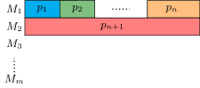
(a) Job cancellation, Processing time reduction.

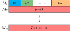
(b) Job arrival, Processing time augmentation, Machine failure.

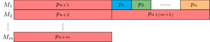
(c) Machine activation.

Figure 7: Schedule $S_{init}$ in the $\mathcal{NP}$-hardness reduction of the makespan recovery problem from $P||C_{\max}$. Different perturbation types are considered individually. The original jobs $J_{1},\ldots,J_{n}$ have processing times $p_{1},\ldots,p_{n}$. Each dummy job $J_{n+1},\ldots,J_{n+(m+1)}$ has processing time $\sum_{j=1}^{n}p_{j}$.

Job Removal, Processing Time Reduction

The initial instance $I_{init}$ consists of $m$ machines, the $n$ original jobs and a dummy job of processing time $p_{n+1}=\sum_{j=1}^{n}p_{j}$. Optimal schedule $S_{init}$ for $I_{init}$ assigns all jobs $J_{1},\ldots,J_{n}$ to machine $M_{1}$, job $J_{n+1}$ to machine $M_{2}$ and leaves $M_{3},\ldots,M_{n}$ empty. We obtain instance $I_{new}$ from $I_{init}$ by removing job $J_{n+1}$ and setting $T_{new}=T$. Since $I_{new}$ consists only of the jobs in $I$, $I_{new}$ admits a feasible schedule of makespan $T_{new}$ iff there exists a schedule of makespan $T$ for $I$. The case of a processing time reduction can be treated similarly, by decreasing $p_{n+1}$ down to $0$ from $\sum_{j=1}^{n}p_{j}$.

Job Arrival, Processing Time Augmentation, Machine Failure

We construct an initial instance $I_{init}$ with $m$ machines, the $n$ original jobs and $m-1$ dummy jobs $J_{n+1},\ldots,J_{n+m-1}$ of processing time $p_{\ell}=\sum_{j=1}^{n}p_{j}$, for $\ell=n+1,\ldots,m-1$. The schedule $S_{init}$ assigning jobs $J_{1},\ldots,J_{n}$ to machine $M_{1}$ and a dummy job to every other machine is optimal for $I_{init}$. We perturb $I_{init}$ by adding job $J_{n+m}$ of processing time $p_{n+m}=\sum_{j=1}^{n}p_{j}$ and setting $T_{new}=\sum_{j=1}^{n}p_{j}+T$. In instance $I_{new}$, we ask the existence of a feasible schedule $S_{new}$ of makespan $T_{new}$. Since $T<\sum_{j=1}^{n}p_{j}$, if such a schedule exists, every pair of dummy jobs must executed by different machines. Thus, $I$ admits a schedule of makespan $T$ iff there exists a schedule with makespan $T_{new}$ for $I_{new}$. For a processing time augmentation and a machine removal, we use the same arguments, but different constructions. In the former case, we add a dummy job $J_{n+m}$ in $I_{init}$ with $p_{n+m}=0$, which becomes $\sum_{j=1}^{n}p_{j}$ in $I_{new}$. In the latter case, we perturb $I_{init}$ by removing $M_{1}$.

Machine Activation

We construct a initial instance $I_{init}$ with $m$ machines, all $n$ original jobs, and $m+1$ dummy jobs $J_{n+1},\ldots,J_{n+(m+1)}$ s.t. $p_{\ell}=\sum_{j=1}^{n}p_{j}$, for $\ell=n+1,\ldots,n+(m+1)$. The initial schedule $S_{init}$ assigns a dummy job and all $n$ original jobs on machine $M_{1}$, two dummy jobs on machine $M_{2}$ and one dummy job on each machine $M_{3},\ldots,M_{m}$. Since any feasible schedule assigning at least two dummy jobs to one machine has makespan $\geq 2\cdot\sum_{j=1}^{n}p_{j}$, $S_{init}$ must be optimal for $I_{init}$. We perturb $I_{init}$ by adding a new machine and setting $T_{new}=\sum_{j=1}^{n}p_{j}+T$. Because $T<\sum_{j=1}^{n}p_{j}$, any feasible schedule for $I_{new}$ of length $T_{new}$ must assign one dummy job to every machine. Thus, there exists a feasible schedule of makespan $T_{new}$ for $I_{new}$ iff $I$ admits a feasible schedule of makespan $T$.  

Appendix C Robustness Analysis for a Single Perturbation

This section completes the proofs of Lemma 4 and Theorem 4 for analyzing the price of robustness of our two-stage approach in the case of a single perturbation.

Lemma 4

Consider a makespan problem instance $(m,\mathcal{J})$ and let $S$ be LexOpt schedule. Given a machine $M_{\ell}\in\mathcal{M}$, denote by $\mathcal{J}^{\prime}$ the subset of all jobs assigned to the machines in $\mathcal{M}\setminus\{M_{\ell}\}$ by $S$. Then, it holds that:

1. $\max_{M_{i}\in\mathcal{M}\setminus\{M_{\ell}\}}\{C_{i}(S)\}=C_{\max}^{*}(m-1,\mathcal{J}^{\prime})$, and

2. $C_{\max}^{*}(m-1,\mathcal{J})\leq 2\cdot C_{\max}^{*}(m,\mathcal{J})$.

Proof:
Suppose that $\max_{M_{i}\in\mathcal{M}\setminus\{M_{\ell}\}}\{C_{i}(S)\}>C_{\max}^{*}(m-1,\mathcal{J}^{\prime})$. Let $S^{*}$ be a minimum makespan schedule for $(m-1,\mathcal{J}^{\prime})$, i.e. $C_{\max}(S^{*})=C_{\max}^{*}(m-1,\mathcal{J}^{\prime})$. By scheduling the jobs in $\mathcal{J}^{\prime}$ as in $S^{*}$ and assigning the jobs in $\mathcal{J}\setminus\mathcal{J}^{\prime}$ to $M_{\ell}$, we obtain a feasible schedule $\widetilde{S}$ for $(m,\mathcal{J})$ s.t. $\widetilde{S}<_{\text{lex}}S$, which is a contradiction. Next, starting from an optimal schedule $S^{*}$ for $(m,\mathcal{J})$, we produce a new schedule $\widetilde{S}$ by moving all jobs of machine $M_{m}$ to machine $M_{m-1}$. Clearly, $\widetilde{S}$ is a feasible for $(m-1,\mathcal{J})$ and the makespan has at most doubled w.r.t. $S^{*}$. Hence, $C_{\max}^{*}(m-1,\mathcal{J})\leq C_{\max}(\widetilde{S})\leq 2\cdot C_{\max}(S^{*})=2\cdot C_{\max}^{*}(m,\mathcal{J})$.  

Theorem 4 (con’t)

For the makespan recovery problem with a single perturbation, Algorithm 3 achieves a tight price of robustness equal to 2, if $S_{init}$ is LexOpt.

Proof:
The proof of the theorem for a processing time reduction or a job removal is presented in the main manuscript. Here, we proceed with the remaining perturbations of Section 2 and show the tightness of our analysis. Let $I_{init}=(m,\mathcal{J})$ be the initial instance with a LexOpt schedule $S_{init}$.

Job Arrival, Processing Time Augmentation

Suppose that $I_{init}$ is perturbed with the arrival of job $J_{n+1}$. The recovered schedule $S_{rec}$ maintains the assignments in $S_{init}$ for $J_{1},\ldots,J_{n}$ and assigns job $J_{n+1}$ to a least loaded machine $M_{\ell}=\arg\min_{M_{i}\in\mathcal{M}}\{C_{i}(S_{init})\}$. In an optimal schedule $S_{new}$ for $I_{new}$, it clearly holds that $C_{\max}(S_{new})\geq\max\{C_{\ell}(S_{new}),p_{n+1}\}$. Consider the auxiliary schedule $\widetilde{S}$ obtained from $S_{new}$ by removing job $J_{n+1}$. Since $\widetilde{S}$ is feasible for $I_{init}$, $C_{\max}(S_{new})\geq C_{\max}(\widetilde{S})\geq C_{\max}(S_{init})$. Hence, $C_{\max}(S_{rec})=\max\{C_{\ell}(S_{init})+p_{n+1},C_{\max}(S_{init})\}\leq C_{\max}(S_{init})+p_{n+1}\leq 2\cdot C_{\max}(S_{new})$. The case where $I_{init}$ is perturbed by increasing $p_{j}$ can be handled using the same arguments and treating the extra piece of $J_{j}$ as a new job assigned to the machine executing $J_{j}$ in $S_{init}$.

Machine Activation, Machine Failure

Consider the case where $I_{init}$ is perturbed because machine $M_{m}$ fails. Let $\mathcal{J}^{\prime}$ be the subset of jobs assigned to $M_{m}$ in $S_{init}$. Clearly, $\sum_{J_{j}\in\mathcal{J}^{\prime}}p_{j}\leq C_{\max}(S_{init})$. The recovered schedule $S_{rec}$ keeps the assignments in $S_{init}$ for the jobs in $\mathcal{J}\setminus\mathcal{J}^{\prime}$ and assigns the jobs in $\mathcal{J}^{\prime}$ to $M_{1},\ldots,M_{m-1}$ using LPT. Thus, $C_{\max}(S_{rec})\leq C_{\max}(S_{init})+\sum_{j\in\mathcal{J}^{\prime}}p_{j}\leq 2\cdot C_{\max}(S_{init})$. Let $S_{new}$ be an optimal schedule for $I_{new}$. Since $I_{new}$ has fewer machines than $I_{init}$, $C_{\max}(S_{init})\leq C_{\max}(S_{new})$. Hence, $C_{\max}(S_{rec})\leq 2\cdot C_{\max}(S_{new})$. In the case where $I_{init}$ is modified with the activation of a new machine $M_{m+1}$, $S_{rec}$ has identical assignments with $S_{init}$, while $M_{m+1}$ is left idle. By Lemma 4.2, $C_{\max}(S_{rec})=C_{\max}^{*}(m,\mathcal{J})\leq 2\cdot C_{\max}^{*}(m+1,\mathcal{J})=2\cdot C_{\max}(S_{new})$.

Tightness

Consider an instance $I_{init}=(m,\mathcal{J})$ with $n=m+1$ jobs of equal processing time $p$. In a LexOpt schedule $S_{init}$, machine $M_{1}$ executes jobs $J_{1}$ and $J_{2}$, machine $M_{i}$ processes job $J_{i+1}$, for $i=2,\ldots,m$, and $C_{\max}(S_{init})=2p$. Assume that $I_{init}$ is disturbed because (i) job $J_{n}$ is removed, (ii) $p_{n}$ is decreased down to zero, or (iii) $M_{m+1}$ is activated. In every case, $C_{\max}(S_{rec})=2p$. However, an optimal schedule $S_{new}$ for $I_{new}$, assigns exactly one job to each machine and $C_{\max}(S_{new})=p$. Next, consider an instance $I_{init}=(m,\mathcal{J})$ with $n=1+(m-1)\cdot m$ jobs, where $p_{1}=m$ and $p_{j}=1$, for $j=2,\ldots,n$. In a LexOpt schedule $S_{init}$, $J_{1}$ is assigned to machine $M_{1}$, exactly $m$ unit jobs are processed by machine $M_{i}$, for $i=1,\ldots,m$, and $C_{\max}(S_{init})=m$. Suppose that $I_{init}$ is perturbed because (i) job $J_{n+1}$ with $p_{n+1}=m$ arrives, (ii) $p_{n}$ is augmented and becomes $m+1$, or (iii) machine $M_{1}$ fails. In each case, $C_{\max}(S_{rec})=2m$. But, in an optimal schedule $S_{new}$ for $I_{new}$, a long job is assigned to the same machine with a unit job, and every other machine contains $m+1$ unit jobs, i.e. $C_{\max}(S_{new})=m+1$.  

Appendix D Robustness Analysis for Multiple Perturbations

This section completes the proofs of Lemma 5 and Theorem 5 for analyzing the price of robustness of our two-stage approach in the case of multiple perturbations.

Lemma 5

Let $(m,\mathcal{J})$ be a makespan problem instance with a LexOpt schedule $S$.

1. If the subset $\mathcal{J}^{\prime}\subseteq\mathcal{J}$ of jobs is executed by the subset $\mathcal{M}^{\prime}\subseteq\mathcal{M}$ of machines in $S$, where $|\mathcal{M}^{\prime}|=m^{\prime}$, then the sub-schedule of $S$ on $\mathcal{M}^{\prime}$ is optimal for $(m^{\prime},\mathcal{J}^{\prime})$, i.e. $\max_{M_{i}\in\mathcal{M}^{\prime}}\{C_{i}(S)\}=C_{\max}^{*}(m^{\prime},\mathcal{J}^{\prime})$.

2. Assuming that $M_{i},M_{\ell}\in\mathcal{M}$ are two different machines such that job $J_{j}\in\mathcal{J}$ is assigned to $M_{i}$ in $S$, then $C_{\ell}(S)\geq C_{i}(S)-p_{j}$.

3. It holds that $C_{\max}^{*}(m-\ell,\mathcal{J})\leq\left(1+\left\lceil\frac{\ell}{m-\ell}\right\rceil\right)\cdot C_{\max}^{*}(m,\mathcal{J})$ $\forall$ $\ell\in\{1,\ldots,m-1\}$.

4. Let $(m,\hat{\mathcal{J}})$ be a makespan problem instance s.t. $\mathcal{J}=\hat{\mathcal{J}}$ and $\frac{1}{f}\cdot\hat{p}_{j}\leq p_{j}\leq\hat{p}_{j}$ for each $J_{j}$, where $p_{j}$ and $\hat{p}_{j}$ is the processing time of $J_{j}$ in $\mathcal{J}$ and $\hat{\mathcal{J}}$, respectively. Then, $\frac{1}{f}\cdot C_{\max}^{*}(m,\hat{\mathcal{J}})\leq C_{\max}^{*}(m,\mathcal{J})\leq C_{\max}^{*}(m,\hat{\mathcal{J}})$.

Proof:
1. Assume for contradiction that $\max_{M_{i}\in\mathcal{M}^{\prime}}\{C_{i}(S)\}>C_{\max}^{*}(m^{\prime},\mathcal{J}^{\prime})$. Starting from an optimal schedule $S^{*}$ for $(m^{\prime},\mathcal{J}^{\prime})$, we construct a feasible schedule $\widetilde{S}$ for $(m,\mathcal{J})$ by assigning the jobs $\mathcal{J}^{\prime}$ as in $S^{*}$ and the jobs $\mathcal{J}\setminus\mathcal{J}^{\prime}$ according to $S$. Then, $\widetilde{S}<_{\text{lex}}S$, which contradicts that $S$ is a LexOpt schedule.

2. Assume for contradiction that $C_{\ell}(S)<C_{i}(S)-p_{j}$, i.e. $C_{\ell}(S)<\max\{C_{\ell}(S)+p_{j},C_{i}(S)-p_{j}\}<C_{i}(S)$. Consider the schedule $\widetilde{S}$ obtained from $S$ by moving $J_{j}$ from $M_{i}$ to $M_{\ell}$. Then, $C_{i}(\widetilde{S})=C_{i}(S)-p_{j}$, $C_{\ell}(\widetilde{S})=C_{\ell}(S)+p_{j}$, and $C_{i^{\prime}}(\widetilde{S})=C_{i^{\prime}}(S)$, for $M_{i^{\prime}}\in\mathcal{M}\setminus\{M_{i},M_{\ell}\}$. That is, $\widetilde{S}<_{lex}S$, which contradicts that $S$ is LexOpt.

3. Starting from an optimal schedule $S^{*}$ for $(m,\mathcal{J})$, we produce a schedule $\widetilde{S}$ by moving all jobs on machines $M_{m-\ell+1},\ldots,M_{m}$ to the remaining machines via round-robin. For $i=1,\ldots,\ell$, the jobs of $M_{m-\ell+i}$ are moved to machine $M_{i\text{ mod }(m-\ell)}$, where $M_{0}=M_{m-\ell}$. Machine $M_{i}\in\{M_{1},\ldots,M_{m-\ell}\}$ receives jobs from at most $\lceil\ell/(m-\ell)\rceil$ machines. Schedule $\widetilde{S}$ uses $m-\ell$ machines and its makespan has increased by a factor at most $1+\lceil\frac{\ell}{m-\ell}\rceil$ w.r.t. $S^{*}$. Hence, $C_{\max}^{*}(m-\ell,\mathcal{J})\leq C_{\max}(\widetilde{S})\leq\left(1+\left\lceil\frac{\ell}{m-\ell}\right\rceil\right)\cdot C_{\max}(S^{*})=\left(1+\left\lceil\frac{\ell}{m-\ell}\right\rceil\right)\cdot C_{\max}^{*}(m,\mathcal{J})$.

4. Starting from an optimal schedule $S^{*}$ for $(m,\mathcal{J})$, we construct a schedule $\hat{S}$ for $(m,\hat{\mathcal{J}})$ with identical assignments. If machine $M_{i}$ executes a job of processing time $p_{j}$ in $S^{*}$, then $M_{i}$ executes a job of processing time $\hat{p}_{j}$ in $\hat{S}$. Since $\frac{1}{f}\cdot\hat{p}_{j}\leq p_{j}\leq\hat{p}_{j}$, we have that $\frac{1}{f}\cdot C_{i}(\hat{S})\leq C_{i}(S^{*})\leq C_{i}(\hat{S})$, for each machine $M_{i}$.  

Theorem 5 (con’t)

For the two-stage robust makespan scheduling problem with $\mathcal{U}(f,k,\delta)$ uncertainty and $k<m$, our LexOpt-based approach achieves a price of robustness:

$$2f\cdot\left(1+\left\lceil\frac{k}{m-k}\right\rceil\right)\cdot(f+k)\cdot\left(1+\left\lceil\frac{\delta}{m}\right\rceil\right).$$

Proof:
The proof for a processing time reduction or a job removal is presented in the main manuscript. Here, we proceed with the remaining perturbations of Section 2 and show the tightness. For analysis purposes, we consider the perturbations in the order of Table 1. To propagate the solution degradation when analyzing each perturbation type, we consider that $C_{\max}(S_{init})\leq\rho C_{\max}(S_{init}^{*})$. That is, the initial schedule $S_{init}$ to be recovered is $\rho$-approximate for $I_{init}$, where $\rho\geq 1$ is arbitrary.

Job Cancellations, Processing Time Reductions (Type 1)

Consider an instance $I_{init}$ with $m$ machines, $(m-k)\cdot m$ jobs of length $f$, and $k$ jobs of length $m\cdot f$, where $f,k=o(m)$. Optimal schedule $S_{init}$ assigns $m$ jobs of length $f$ on each of the first $m-k$ machines, one job of length $m\cdot f$ on each of the remaining $k$ machines, and has makespan $C_{\max}(S_{init})=m\cdot f$. We perturb $I_{init}$ by decreasing the processing time of each job assigned to $M_{2},\ldots,M_{m-k}$ down to 1, and cancelling the jobs assigned to the last $k$ machines. The recovered schedule has makespan $C_{\max}(S_{rec})=m\cdot f$. But an optimal schedule $S_{new}$ assigns to each machine a job of length $f$ and $m-k-1$ unit-length jobs, i.e. $C_{\max}(S_{new})=(m-k-1)+f$. Figure 8 illustrates this tightness example, where $\frac{C_{\max}(S_{rec})}{C_{\max}(S_{new})}=\frac{m\cdot f}{(m-k-1)+f}=\frac{m\cdot f}{(m-k)\left(1+\frac{f-1}{m-k}\right)}=O((1+\frac{k}{m-k})f)$.

(a) LexOpt schedule $S_{init}$.

(b) Recovered schedule $S_{rec}$.

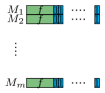
(c) Optimal schedule $S_{new}$.

Figure 8: Makespan recovery instance for which the $O(f\cdot(1+\lceil\frac{k}{m-k}\rceil))$ factor is tight under job cancellations and processing time reductions.

Processing Time Augmentations (Type 2)

Recall that job $J_{j}\in\mathcal{J}$ is stable if $\hat{p}_{j}\leq fp_{j}$ and unstable if not. Also, let $F=\max_{J_{j}\in\hat{\mathcal{J}}}\{\hat{p}_{j}\}$. Since $I_{new}$ $\in\mathcal{U}(f,k,\delta)$, at most $k$ processing times become equal to $F$ and all remaining jobs are increased by a factor at most $f$. Given that $S_{rec}$ is identical with $S_{init}$, except that some processing times are increased, $C_{i}(S_{rec})\leq f\cdot C_{i}(S_{init})+k\cdot F$ for each $M_{i}\in\mathcal{M}$. Given an optimal schedule $S_{init}^{*}$ for $I_{init}$ and that the processing times in $I_{new}$ are one-to-one greater than or equal to the ones in $I_{init}$, $C_{i}(S_{init})\leq\rho\cdot C_{\max}(S_{init}^{*})\leq\rho\cdot C_{\max}(S_{new})$. In addition, $C_{\max}(S_{new})\geq F$. Hence, $C_{\max}(S_{rec})\leq(f+k)\rho\cdot C_{\max}(S_{new})$.

For the tightness, consider instance $I_{init}$ (Figure 9) with $m$ machines and $n=m^{2}$ unit-length jobs. In $S_{init}$, each machine executes $m$ jobs and $C_{\max}(S_{init})=m$. After uncertainty realization, $k$ jobs assigned to $M_{1}$ get processing time $F$, every other job on $M_{1}$ gets processing time $f$, and all other processing times remain the same in $I_{init}$ and $I_{new}$. Suppose that $F=f+m$, $F=\Theta(m)$, $f=o(m)$ and $k=o(m)$. Schedule $S_{rec}$ performs identical assignments with $S_{init}$, i.e. $C_{\max}(S_{rec})=k\cdot F+(m-k)\cdot f$. In an optimal schedule $S_{new}$ for $I_{new}$, each machine $M_{i}$ with $i\leq k$ processes a job of length $F$ and $k$ unit length jobs, while each machine $M_{i}$ with $i>k$ executes a job of length $f$ and $m+k$ unit length jobs, i.e. $C_{\max}(S_{new})=F+m$. Thus, $\frac{C_{\max}(S_{rec})}{C_{\max}(S_{new})}=\frac{k\cdot F}{F+k}+\frac{(m-k)\cdot f}{f+m+k}=k\cdot\frac{1}{1+\frac{k}{F}}+f\cdot\frac{1}{1+\frac{f+2k}{m-k}}=O(f+k)$.

(a) LexOpt schedule $S_{init}$.

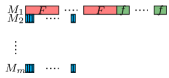
(b) Recovered schedule $S_{rec}$.

(c) optimal schedule $S_{new}$.

Figure 9: Makespan recovery instance for which the $O(f+k)$ factor is tight under processing time augmentations.

Machine Activations (Type 3)

Denote by $\mathcal{M}^{s}$ the set of available machines in $S_{init}$ and by $\mathcal{M}^{u}$ the set of newly activated machines after uncertainty realization. Algorithm 3 keeps the schedule $S_{init}$ for the machines in $\mathcal{M}^{s}$ and leaves the machines in $\mathcal{M}^{u}$ idle, i.e. $C_{\max}(S_{rec})\leq\rho\cdot C_{\max}^{*}(m,\mathcal{J})$. By definition, $C_{\max}(S_{new})=C_{\max}^{*}(m+k,\mathcal{J})$. Hence, by Lemma 5.3, we conclude that $C_{\max}(S_{rec})\leq(1+\lceil k/m\rceil)\rho\cdot C_{\max}(S_{new})$. For the tightness of this bound, consider an instance with $m$ machines and $n=m\cdot(m+k)$ unit jobs. In $S_{init}$, each machine processes $m+k$ unit jobs and $C_{\max}(S_{init})=m+k$. In $S_{rec}$, all newly activated machines are empty and $C_{\max}(S_{rec})=m+k$. But an optimal schedule $S_{new}$ for $I_{new}$ assigns exactly $m$ jobs on each machine, i.e. $C_{\max}(S_{new})=m$. That is, $\frac{C_{\max}(S_{rec})}{C_{\max}(S_{init})}=1+\frac{k}{m}$.

Job Arrivals, Machine Failures (Type 4)

Consider a set of free jobs arriving after uncertainty realization. Algorithm 3 schedules these jobs according to LPT. We partition the set $\mathcal{M}$ of machines into the set $\mathcal{M}^{s}$ of stable machines, not executing free jobs, and the set $\mathcal{M}^{u}$ of unstable machines, assigned free jobs, in $S_{rec}$. Since $\mathcal{J}_{init}\subset\mathcal{J}_{new}$ and $\mathcal{M}_{init}=\mathcal{M}_{new}$, if there is a machine $M_{i}\in\mathcal{M}^{s}$ with $C_{i}(S_{rec})=C_{\max}(S_{rec})$, then $C_{\max}(S_{rec})=C_{\max}(S_{init})\leq\rho\cdot C_{\max}^{*}(I_{init})\leq\rho\cdot C_{\max}(S_{new})$. If there is not such a machine in $\mathcal{M}^{s}$, we use the analysis for LPT by Graham [27]. Since the last completing job $J_{j}$ begins at $b_{j}$, all machines are occupied until $b_{j}$ in $S_{rec}$. Thus, $C_{\max}(S_{rec})=b_{j}+p_{j}\leq\frac{1}{m}\sum_{J_{j^{\prime}}\in\mathcal{J}_{new}}p_{j^{\prime}}+p_{j}\leq 2\cdot C_{\max}(S_{new})$. In both cases, $C_{\max}(S_{rec})\leq\max\{2,\rho\}\cdot C_{\max}(S_{new})$. The case where a machine $M_{i}\in\mathcal{M}$ fails can be treated similarly by considering the jobs originally assigned to $M_{i}$ in $S_{init}$ as free. In the case where $\rho>2$, we may design a makespan problem instance such that the arrival of a new job with a tiny processing time has the effect that the recovered schedule remains $\rho$-approximate. The tightness example for LPT implies that Algorithm 3 cannot result in a price of robustness better than 2.  

Appendix E Flexible Recovery Strategy

Next, we present a more flexible recovery strategy (than Algorithm 3) that modifies a bounded number of binding decisions [18, 43]. To this end, we formulate the makespan recovery problem as a MILP. Let $\mathcal{J}^{B}=\{J_{j}\in\mathcal{J}_{init}\cap\mathcal{J}_{new}:\exists i\text{ with }x_{i,j}(S_{\text{init}})=1\}$ be the binding decisions, i.e. the jobs appearing both in $I_{init}$ and $I_{new}$. Algorithm 3 keeps the assignments in $S_{init}$ for the binding jobs $\mathcal{J}^{B}$ and greedily schedules the free jobs $\mathcal{J}^{F}=\mathcal{J}\setminus\mathcal{J}^{B}$ with LPT to produce $S_{rec}$. A more flexible recovery strategy migrates a bounded number $g$ of binding jobs. These migrations produce better recovered solutions at the price of extra computational effort and higher transformation cost. Denote by $\mathcal{J}_{i}^{B}\subseteq\mathcal{J}^{B}$ and $\mu_{j}$ the subset of binding jobs assigned to machine $M_{i}$ and the machine index which job $J_{j}\in\mathcal{J}^{B}$ is assigned to, respectively, in $S_{init}$. Our flexible recovery strategy solves MILP (1) with the additional constraint $\sum_{J_{j}\in\mathcal{J}^{B}}\sum_{M_{i}\in\mathcal{M}\setminus\{M_{\mu_{j}}\}}x_{i,j}\leq g$.

Appendix F Numerical Results with Degenerate Instances

This section complements our numerical results with degenerate instances of $P||C_{\max}$. Section F.1 describes the generation of these instances. Sections F.2-F.3 evaluate the LexOpt branch-and-bound algorithm and the robustness of our two-stage approach using the new instances.

F.1 Generation of Degenerate Instances

Degenerate instances have less balanced optimal solutions than well-formed instances. To produce degenerate instances, we sample integer processing times that can be encoded with $b$ bits. Instances with small $\kappa=b/n$ values are easier to solve than instances with larger $\kappa$ values [4]. The phase transition from “easy” to “hard” instances becomes sharper as $n$ increases and occurs at the threshold value $\kappa^{*}=\frac{\log_{2}m}{m-1}$. Instances with small $\kappa$ admit exponentially many perfect solutions (where all machine completion times are equal). Instances with $\kappa>\kappa^{*}$ have less or no perfect solutions. Similar phase transitions occur for other fundamental combinatorial optimization problems, e.g. satisfiability [39] and the traveling salesman problem [24], where instances near the threshold value tend to be the most difficult.

We derive degenerate instances by varying two parameters: (i) the number $m$ of machines and (ii) the number $n$ of jobs. Further, we use a processing time seed $q=2^{\lfloor\kappa(m)\cdot n\rfloor}$ with $\kappa(m)=(\log_{2}m)/(m-1)$. Table 3 reports this information for moderate and intermediate degenerate instances. For each combination of $m$, $n$ and the corresponding $q=2^{\lfloor\kappa(m)\cdot n\rfloor}$ value, we generate 3 instances by sampling processing times from the set $\{1,\ldots,q\}$ using the uniform, normal and symmetric of normal distributions, similarly to the well-formed instances.

Table 3: Degenerate Instances

Instances	$\mathbf{m}$	$\mathbf{n}$	$\mathbf{q}$
Moderate	3	$20,25,30,35$	$2^{15},2^{19},2^{23},2^{27}$
	4	$25,30,35,40$	$2^{16},2^{20},2^{23},2^{26}$
	5	$30,35,40,45$	$2^{17},2^{20},2^{23},2^{26}$
	6	$35,40,45,50$	$2^{18},2^{20},2^{23},2^{25}$
Intermediate	10	$40,50,60,70$	$2^{14},2^{18},2^{22},2^{25}$
	12	$45,55,65,75$	$2^{14},2^{17},2^{21},2^{24}$
	14	$55,65,75,85$	$2^{16},2^{19},2^{21},2^{24}$
	16	$60,70,80,90$	$2^{16},2^{18},2^{21},2^{24}$

F.2 LexOpt Branch-and-Bound Algorithm Evaluation

We evaluate our branch-and-bound algorithm on degenerate instances in comparison with the sequential, weighting and highest-rank objective methods. For MILP solving, we use (i) $10^{3}$ CPU seconds time limit and (ii) $10^{-4}$ error tolerance, similarly to the numerical results obtained with well-formed instances. Figure 10 shows performance profiles for evaluating the running times and quality of computed solutions on degenerate instances. We observe that degenerate instances are significantly harder to solve than well-formed instances of identical size. For instance, no solver converges for any intermediate degenerate instance, while every solver converges for $>30\%$ of the intermediate well-formed instances. In terms of solver comparison, we derive similar results to those obtained for well-formed instances. The sequential method performs similarly to the weighting method. The highest-rank objective method produces the best heuristic results. Our branch-and-bound method produces the second best heuristic result for intermediate degenerate instances and computes LexOpt solutions quickly when it terminates.

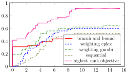
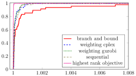
(a) Moderate instances: time (s) on $\log_{2}$ scale (left), upper bounds on $[1,1.008]$ (right).

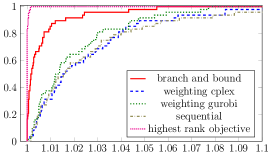
(b) Intermediate instances: upper bounds on $[1,1.1]$. No solver converges for any intermediate degenerate instance within the specified time limit.

Figure 10: Performance profiles for the degenerate test set with $10^{3}$ s timeout.

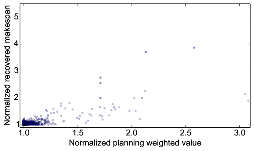
(a) Binding Recovery

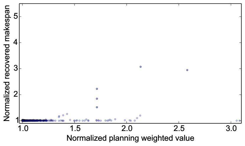
(b) Flexible Recovery

Figure 11: Degenerate instances scatter plots illustrating the recovered solution makespan with respect to the initial solution weighted value.

F.3 Two-Stage Robustness Assessment

Next, we investigate the impact of LexOpt to the quality of the recovered solution for degenerate instances. For each degenerate instance $I_{init}$ derived according to Section F.1, we compute 50 diverse initial solutions using the CPLEX solution pool feature. To quantify the closeness of an initial solution to LexOpt, we use the weighted value $W(S)=\sum_{i=1}^{m}B^{m-i}\cdot C_{i}(S)$. Further, we obtain a perturbed instance $I_{new}$ by generating random disturbances, similarly to well-formed instances. Then, we fix every initial solution by applying our binding and flexible recovery strategies in Section 4.1. As in the case of well-formed instances, Figures 11(a) and 11(b) plot the normalized makespan $C^{N}(S_{rec})$ obtained by our recovery strategies and the normalized initial solution weighted value $W^{N}(S_{init})$ for every recovered solution. Clearly, the recovered solution improves if the initial solution weighted value decreases. Moreover, flexibility enables more efficient recovery. Interestingly, degenerate instances are recovered more efficiently than well-formed ones.

Appendix G Table of Notation

Table 4: Nomenclature

Name	Description
Makespan scheduling problem
$I=(m,\mathcal{J})$	Instance
$i,q,\mu$	Machine indices ($q,\mu$ typically used as auxiliary machine indices)
$j,h,\ell$	Job indices ($h,\ell$ typically used as auxiliary job indices)
$m$	Number of machines
$M_{i}\in\mathcal{M}$	Machine $M_{i}$ in the set $\mathcal{M}=\{M_{1},\ldots,M_{m}\}$ of all machines
$n$	Number of jobs
$J_{j}\in\mathcal{J}$	Job $J_{j}$ in the set $\mathcal{J}\in\{J_{1},\ldots,J_{n}\}$ of all jobs
$p_{j}$	Processing time of job $J_{j}$
$C_{\max}$	Makespan
$C_{i}$	Completion time of machine $M_{i}$
$x_{i,j}$	Binary variable indicating an assignment of job $J_{j}$ to machine $M_{i}$
$S=(\vec{y},\vec{C}),S^{\prime},\widetilde{S}$	Schedules ($S^{\prime},\widetilde{S}$ typically used as auxiliary schedules)
$S^{*}$	LexOpt schedule
$\mathcal{S}$	Set of all feasible schedules
LexOpt scheduling problem
$\leq_{\text{lex}}$	Operator for lexicographic comparison
$F_{i}$	$i$-th greatest completion time, i.e. $i$-th objective function
$v_{i}^{*}$	Value of $F_{i}$ in a LexOpt schedule $S^{*}$
$\mathcal{T}_{q}$	Set of tuples $(i_{1},\ldots,i_{q})$ with $q$ pairwise disjoint machine indices
$w_{i}$	Weight of objective function $F_{i}$ (weighting method)
$\mathcal{P}$	Solution pool (highest-rank objective method)
Branch-and-bound algorithm
$Q$	Stack of visited unexplored nodes
$I$	Incumbent, i.e. lexicographically best-found solution
$u,v,r$	Nodes ($r$ is the root) in the branch-and-bound tree
$\mathcal{S}(u)$	Feasible solutions below node $u$ in the branch-and-bound tree
$\ell$	Node level, i.e. job index, in the branch-and-bound tree
$t_{i}$	Partial completion time of machine $M_{i}$ in a branch-and-bound node
$\mathcal{R}$	Subset of jobs scheduled below a branch-and-bound node
$L_{i},\vec{L}$	Component $L_{i}$ of vectorial lower bound $\vec{L}=(L_{1},\ldots,L_{m})$
$U_{i},\vec{U}$	Component $U_{i}$ of vectorial upper bound $\vec{U}=(U_{1},\ldots,U_{m})$
$\tau$	Time point
$\tilde{p}_{j}$	Piece of job $J_{j}$
$\lambda,\Lambda$	Amount of processing time load
Makespan recovery problem
$I_{init}$	Initial instance $(m_{init},\mathcal{J}_{init})$
$I_{new}$	Perturbed instance $(m_{new},\mathcal{J}_{new})$
$S_{init}$	Initial optimal schedule for $I_{init}$
$S_{rec}$	Recovered schedule for $I_{new}$
$S_{new}$	Optimal schedule for $I_{new}$
$\rho$	Approximation ratio
Uncertainty modeling
$\mathcal{U}(f,k,\delta)$	Uncertainty set
$f$	Perturbation factor
$k$	Number of unstable jobs
$\delta$	Number of new machines
$C_{\max}^{*}(m,\mathcal{J})$	Optimal objective value of makespan problem instance $(m,\mathcal{J})$
Binding recovery strategy
$T$, $T_{new}$	Target makespan for instance $I$ and perturbed instance $I_{new}$
$T_{new}$	Target makespan for perturbed instance $I_{new}$
$\mathcal{M}^{\prime}$	Subset of machines
$m^{\prime}$	Number of machines in $\mathcal{M}^{\prime}$
$\mathcal{J}^{\prime}$	Subset of jobs
$\eta$	Reduction of $p_{j}$
$(\hat{m},\hat{\mathcal{J}})$	Neighboring instance of $(m,\mathcal{J})$
$\hat{p}_{j}$	Processing time of job $J_{j}$ in $(\hat{m},\hat{\mathcal{J}})$
$\mathcal{M}^{s},\mathcal{M}^{u}$	Stable machines $\mathcal{M}^{s}$ and unstable machines $\mathcal{M}^{u}=\mathcal{M}\setminus\mathcal{M}^{s}$
$m^{s},m^{u}$	Number of stable ($m^{s}$) and unstable ($m^{u}$) machines
$\mathcal{J}_{init}^{s}$	Subset of stable jobs in $I_{init}$
$\mathcal{J}_{new}^{s}$	Subset of stable jobs in $I_{new}$
$F$	Maximum processing time in $I_{new}$
Flexible recovery strategy
$\mathcal{J}^{B},\mathcal{J}^{F}$	Subset of binding ($\mathcal{J}^{B}$) and free ($\mathcal{J}^{F}=\mathcal{J}\setminus\mathcal{J}^{B}$) jobs
$\mathcal{J}_{i}^{B}$	Binding jobs originally assigned to machine $M_{i}$
$\mu_{j}$	Machine executing job $J_{j}$ in $S_{init}$
$g$	Limit on migrations of binding job
Numerical results
$\kappa$	Phase transition parameter
$\kappa^{*}$	Critical value of phase transition parameter
$b$	Number of bits for generating processing times
$q$	Processing time seed
$\mathcal{U}$	Discrete uniform distribution
$\mathcal{N}$	Normal distribution
$W$	Weighted value, i.e. weighted sum of objective functions
$Ub,Lb$	Best-found incumbent ($Ub$) and lower bound ($Lb$)
$d_{m},d_{n}$	Number of machine ($d_{m}$) and job ($d_{n}$) disturbances
$W^{N}$	Normalized weighted value
$W^{*}$	Best computed weighted value
$C_{\max}^{N}$	Normalized makespan
$C_{\max}^{*}$	Best recovered makespan

References

- Adams et al. [2016] Adams, W., Belotti, P., & Shen, R. (2016). Convex hull characterizations of lexicographic orderings. J Glob Optim, 66, 311–329.
- Ausiello et al. [2011] Ausiello, G., Bonifaci, V., & Escoffier, B. (2011). Complexity and approximation in reoptimization. In S. B. Cooper, & A. Sorbi (Eds.), Computability in Context chapter 4. (pp. 101–129). Imperial College Press.
- Balas et al. [2012] Balas, E., Fischetti, M., & Zanette, A. (2012). A hard integer program made easy by lexicography. Math Program, 135, 509–514.
- Bauke et al. [2003] Bauke, H., Mertens, S., & Engel, A. (2003). Phase transition in multiprocessor scheduling. Physical Review Letters, 90, 158701.
- Ben-Tal et al. [2009] Ben-Tal, A., Ghaoui, L. E., & Nemirovski, A. (2009). Robust optimization. Princeton University Press.
- Ben-Tal et al. [2004] Ben-Tal, A., Goryashko, A., Guslitzer, E., & Nemirovski, A. (2004). Adjustable robust solutions of uncertain linear programs. Math Program, 99, 351–376.
- Bender et al. [2015] Bender, M. A., Farach-Colton, M., Fekete, S. P., Fineman, J. T., & Gilbert, S. (2015). Reallocation problems in scheduling. Algorithmica, 73, 389–409.
- Bertsimas et al. [2011] Bertsimas, D., Brown, D. B., & Caramanis, C. (2011). Theory and applications of robust optimization. SIAM Review, 53, 464–501.
- Bertsimas & Caramanis [2010] Bertsimas, D., & Caramanis, C. (2010). Finite adaptability in multistage linear optimization. IEEE Transactions on Automatic Control, 55, 2751–2766.
- Bertsimas & Georghiou [2018] Bertsimas, D., & Georghiou, A. (2018). Binary decision rules for multistage adaptive mixed-integer optimization. Math Program, 167, 395–433.
- Bertsimas & Sim [2003] Bertsimas, D., & Sim, M. (2003). Robust discrete optimization and network flows. Math Program, 98, 49–71.
- Bertsimas & Sim [2004] Bertsimas, D., & Sim, M. (2004). The price of robustness. Oper Res, 52, 35–53.
- Bougeret et al. [2019] Bougeret, M., Pessoa, A. A., & Poss, M. (2019). Robust scheduling with budgeted uncertainty. Discrete Applied Mathematics, 261, 93–107.
- Bouveret & Lemaître [2009] Bouveret, S., & Lemaître, M. (2009). Computing leximin-optimal solutions in constraint networks. Artificial Intelligence, 173, 343–364.
- Brucker [2007] Brucker, P. (2007). Scheduling algorithms (5th Ed.). Springer.
- Burkard & Rendl [1991] Burkard, R. E., & Rendl, F. (1991). Lexicographic bottleneck problems. Oper Res Lett, 10, 303–308.
- Chassein & Goerigk [2016] Chassein, A., & Goerigk, M. (2016). On the recoverable robust traveling salesman problem. Optimization Letters, 10, 1479–1492.
- Chassein et al. [2018] Chassein, A., Goerigk, M., Kasperski, A., & Zieliński, P. (2018). On recoverable and two-stage robust selection problems with budgeted uncertainty. Eur J Oper Res, 265, 423 – 436.
- Cramer & Pollatschek [1979] Cramer, J., & Pollatschek, M. A. (1979). Candidate to job allocation problem with a lexicographic objective. Manage Sci, 25, 466–473.
- Dolan & Moré [2002] Dolan, E. D., & Moré, J. J. (2002). Benchmarking optimization software with performance profiles. Math Program, 91, 201–213.
- Ehrgott [2006] Ehrgott, M. (2006). Multicriteria optimization. Springer.
- Fischetti et al. [2009] Fischetti, M., Lodi, A., & Salvagnin, D. (2009). Just MIP it! In Matheuristics (pp. 39–70). Springer.
- Fischetti & Toth [1988] Fischetti, M., & Toth, P. (1988). A new dominance procedure for combinatorial optimization problems. Oper Res Lett, 7, 181–187.
- Gent & Walsh [1996] Gent, I. P., & Walsh, T. (1996). The TSP phase transition. Artif Intell, 88, 349–358.
- Georgiadis et al. [2002] Georgiadis, L., Georgatsos, P., Floros, K., & Sartzetakis, S. (2002). Lexicographically optimal balanced networks. IEEE/ACM T Network, 10, 818–829.
- Goerigk & Schöbel [2016] Goerigk, M., & Schöbel, A. (2016). Algorithm engineering in robust optimization. In L. Kliemann, & P. Sanders (Eds.), Algorithm Engineering - Selected Results & Surveys (pp. 245–279). Springer volume 9220 of Lecture Notes in Computer Science.
- Graham [1969] Graham, R. L. (1969). Bounds on multiprocessing timing anomalies. SIAM Journal on Applied Mathematics, 17, 416–429.
- Gupta & Maravelias [2019] Gupta, D., & Maravelias, C. T. (2019). On the design of online production scheduling algorithms. Comput Chem Eng, 129, 106517.
- Gupta et al. [2016] Gupta, D., Maravelias, C. T., & Wassick, J. M. (2016). From rescheduling to online scheduling. Chem Eng Res Des, 116, 83–97.
- Gupte [2016] Gupte, A. (2016). Convex hulls of superincreasing knapsacks and lexicographic orderings. Discrete Applied Mathematics, 201, 150–163.
- Hanasusanto et al. [2015] Hanasusanto, G. A., Kuhn, D., & Wiesemann, W. (2015). K-adaptability in two-stage robust binary programming. Oper Res, 63, 877–891.
- Kasperski & Zielinski [2014] Kasperski, A., & Zielinski, P. (2014). Minmax (regret) scheduling problems. Sequencing and scheduling with inaccurate data, (pp. 159–210).
- Kouvelis & Yu [2013] Kouvelis, P., & Yu, G. (2013). Robust discrete optimization and its applications volume 14. Springer Science & Business Media.
- Letsios & Misener [2017] Letsios, D., & Misener, R. (2017). Source code. https://github.com/cog-imperial/two_stage_scheduling.
- Leung [2004] Leung, J. Y. (Ed.) (2004). Handbook of Scheduling - Algorithms, Models, and Performance Analysis. Chapman and Hall - CRC.
- Liebchen et al. [2009] Liebchen, C., Lübbecke, M., Möhring, R., & Stiller, S. (2009). The concept of recoverable robustness, linear programming recovery, and railway applications. In Robust and online large-scale optimization (pp. 1–27). Springer.
- Luss [1999] Luss, H. (1999). On equitable resource allocation problems: A lexicographic minimax approach. Oper Res, 47, 361–378.
- Mistry et al. [2018] Mistry, M., D’Iddio, A. C., Huth, M., & Misener, R. (2018). Satisfiability modulo theories for process systems engineering. Comput Chem Eng, 113, 98–114.
- Mitchell et al. [1992] Mitchell, D. G., Selman, B., & Levesque, H. J. (1992). Hard and easy distributions of SAT problems. In AAAI. San Jose, CA. (pp. 459–465).
- Monaci & Pferschy [2013] Monaci, M., & Pferschy, U. (2013). On the robust knapsack problem. SIAM J Optim, 23, 1956–1982.
- Muldoon et al. [2013] Muldoon, F. M., Adams, W. P., & Sherali, H. D. (2013). Ideal representations of lexicographic orderings and base-2 expansions of integer variables. Oper Res Lett, 41, 32–39.
- Nace & Orlin [2007] Nace, D., & Orlin, J. B. (2007). Lexicographically minimum and maximum load linear programming problems. Oper Res, 55, 182–187.
- Nasrabadi & Orlin [2013] Nasrabadi, E., & Orlin, J. B. (2013). Robust optimization with incremental recourse. Preprint arXiv, 1312.4075.
- Ogryczak [1997] Ogryczak, W. (1997). On the lexicographic minimax approach to location problems. Eur J Oper Res, 100, 566–585.
- Pardalos et al. [2016] Pardalos, P. M., Žilinskas, A., & Žilinskas, J. (2016). Non-convex multi-objective optimization. Springer.
- Phillips et al. [2017] Phillips, A. E., Walker, C. G., Ehrgott, M., & Ryan, D. M. (2017). Integer programming for minimal perturbation problems in university course timetabling. Annals of Operations Research, 252, 283–304.
- Salvagnin [2005] Salvagnin, D. (2005). A dominance procedure for integer programming. Master thesis, University of Padua.
- Sanders et al. [2009] Sanders, P., Sivadasan, N., & Skutella, M. (2009). Online scheduling with bounded migration. Mathematics of Operations Research, 34, 481–498.
- Schieber et al. [2018] Schieber, B., Shachnai, H., Tamir, G., & Tamir, T. (2018). A theory and algorithms for combinatorial reoptimization. Algorithmica, 80, 576–607.
- Schmeidler [1969] Schmeidler, D. (1969). The nucleolus of a characteristic function game. SIAM J Appl Math, 17, 1163–1170.
- Sherali [1982] Sherali, H. D. (1982). Equivalent weights for lexicographic multi-objective programs: Characterizations & computations. Eur J Oper Res, 11, 367–379.
- Sherali & Soyster [1983] Sherali, H. D., & Soyster, A. L. (1983). Preemptive and non-preemptive multiobjective programming: relationships and counter examples. J Optim Theory Appl, 39, 173–186.
- Skutella & Verschae [2016] Skutella, M., & Verschae, J. (2016). Robust polynomial-time approximation schemes for parallel machine scheduling with job arrivals and departures. Math Oper Res, 41, 991–1021.
- Soyster [1973] Soyster, A. L. (1973). Convex programming with set-inclusive constraints and applications to inexact linear programming. Oper Res, 21, 1154–1157.
- Verschae [2012] Verschae, J. (2012). The Power of Recourse in Online Optimization. Ph.D. thesis Technische Universität Berlin, Germany.
- Wiebe et al. [2018] Wiebe, J., Cecílio, I., & Misener, R. (2018). Data-driven optimization of processes with degrading equipment. Ind Eng Chem Res, 57, 17177–17191.
- Yu & Shi [2007] Yu, Z., & Shi, W. (2007). An adaptive rescheduling strategy for grid workflow applications. In IPDPS (pp. 1–8). IEEE.
- Zufiria & Álvarez-Cubero [2017] Zufiria, P. J., & Álvarez-Cubero, J. A. (2017). Generalized lexicographic multiobjective combinatorial optimization. Application to cryptography. SIAM J Optim, 27, 2182–2201.