Approximate Hamiltonian for baryons in heavy-flavor QCD

Abstract

Aiming at relativistic description of gluons in hadrons, the renormalization group procedure for effective particles (RGPEP) is applied to baryons in QCD of heavy quarks. The baryon eigenvalue problem is posed using the Fock-space Hamiltonian operator obtained by solving the RGPEP equations up to second order in powers of the coupling constant. The eigenstate components that contain three quarks and two or more gluons are heuristically removed at the price of inserting a gluon-mass term in the component with one gluon. The resulting problem is reduced to the equivalent one for the component of three quarks and no gluons. Each of the three quark-quark interaction terms thus obtained consists of a spin-dependent Coulomb term and a spin-independent harmonic oscillator term. Quark masses are chosen to fit the lightest spin-one quarkonia masses most accurately. The resulting estimates for bbb and ccc states match estimates obtained in lattice QCD and in quark models. Masses of ccb and bbc states are also estimated. The corresponding wave functions are invariant with respect to boosts. In the ccb states, charm quarks tend to form diquarks. The accuracy of our approximate Hamiltonian can be estimated through comparison by including components with two gluons within the same method.

1 Introduction

Theoretically precise and phenomenologically accurate description of triply-heavy baryons as quantum states of quarks and gluons requires the formulation of QCD that satisfies several conditions. It ought to include a construction of the theory ground state, or vacuum, whose excitations are the quanta of quark and gluon fields. Since the canonical QCD Hamiltonian involves singularities and requires regularization, the theoretical formulation should include a mathematically precise renormalization procedure with clear physical interpretation, as a foundation of its predictability. The condition that individually quarks and gluons are not observed, implies that the formulation should allow for inclusion of confinement. The fact that heavy baryons may participate in processes whose description involves motion with speeds close to the speed of light, forces the formulation to be relativistic. In particular, it must guarantee description of baryons that have energies very much larger than their masses. Finally, knowing technical complexity of QCD and realizing that exact solutions are unlikely, it is necessary to demand that the formulation includes an outline of a process of successive approximations that stand a chance of systematically improving precision and accuracy of approximate solutions for observables. This article concerns a pilot application of an approach to heavy-quark QCD that in principle satisfies these requirements.

Quark model represented baryons as bound states of three quarks, e.g. see Capstick:2000qj ; Capstick:1986bm . In QCD, baryons are instead superpositions of states of quanta of quark and gluon fields. A priori, the number of quanta varies from three to infinity, across an infinite set of components. These quanta may have momenta ranging from zero to infinity. Their interactions diverge with their momenta. This article contributes to a development of a Hamiltonian approach to QCD that appears capable of filling the gap between the complex quantum-field picture and simple quark-model picture for hadrons QQbarRGPEP . Most succinctly, we illustrate a new method for solving the bound-state problem in canonical quantum field theories with asymptotic freedom in terms of its first application to the case of baryons in heavy-flavor QCD. Our method involves three consecutive steps: we solve our renormalization group equation for the front form (FF) Hamiltonian of the theory using the concept of effective particles in the Fock space; we reduce the resulting heavy-baryon eigenvalue problem for low-mass eigenstates to the eigenvalue problem solely for their Fock component of three effective quarks, using a gluon mass ansatz to account for the Fock components with more effective gluons than one; and we draw a qualitative sketch of the estimated low-mass heavy baryons spectrum that follows from the dominant mechanism of binding, while spin and other relatively small corrections to the effects of dominant interactions require future more elaborate calculations of higher-order using the same method. The theoretical challenge our method thus addresses is how to represent states of heavy baryons in terms of the Fock-space wave-functions for quarks and gluons that are invariant with respect to Lorentz boosts. The new results that our pilot study yields for heavy baryons, including the approximate analytic formulae for their mass eigenvalues and corresponding boost-invariant wave functions that can be used in phenomenology of their production and detection, are thus derived in full detail from the heavy-flavor QCD supplied with our gluon mass ansatz. However, our pilot study of the low-mass triply heavy baryons involves severe simplifications. Similar simplifications are made in other approaches but without using the concept of effective particles that we introduce. In our approach, all the simplifications we make in the pilot study can be systematically removed within the same method while increasing its precision, as will be explained later on, but we do not address the question if the RGPEP may be used to derive the pNRQCD, which would require comparison of the dimensional regularization renormalization group equations with equations of the RGPEP, see the pertinent footnote on p. 456 in Ref. tHooft:1973mfk .

We limit the theory to quarks that have masses much greater than $\Lambda_{QCD}$, excluding the top quark, and we consider the weak coupling limit Wilsonetal . Creation of quark-antiquark pairs is neglected. Components with more than one gluon are eliminated, by assuming that their dominant effect in the component with one gluon is that the gluon has a mass, allowed to be a function of the gluon kinematic relative momentum with respect to the quarks. We use second-order perturbation theory to derive the resulting effective Hamiltonian for baryons that only acts in the component with three quarks. We compare the quark-quark interaction terms in this Hamiltonian to similar terms in the Hamiltonian that only acts in the quark-anti-quark component in quarkonia, previously derived using the same method QQbarRGPEP . Masses of heavy baryons are estimated by solving the resulting eigenvalue equation in the nonrelativistic limit. The parameters involved (the running coupling and the quark masses) are chosen using heavy quarkonia experimental data. In this way, our estimates for baryon masses contain no new parameters. More precisely, the coupling constant is extrapolated from a formally infinitesimal value of weak-coupling limit to the value implied at the quark-mass scale by the known coupling constant at the scale of $Z$-boson mass. Quark masses are adjusted to the known spectra of heavy quarkonia. The scale parameter for hadrons built from different flavors is fixed by a linear interpolation between its one-flavor values. This will be explained in detail later.

The concept of effective-gluon mass that we use is explained in Sec. 2, followed by a brief outline of our method in Sec. 3. The method is called the renormalization group procedure for effective particles (RGPEP). Our concept of the gluon mass differs from the concepts discussed in the literature, see, e.g., Refs. Parisi:1980jy ; Cornwall:1981zr ; Aguilar:2017dco . The second-order baryon eigenvalue problem is outlined in Sec. 4. Details of the effective quark-quark interaction terms in $ccc$ and $bbb$ baryons, implied by the gluon mass, are described in Sec. 5, including a comparison with the case of heavy quarkonia. Sec. 6 extends the calculation to the $ccb$ and $bbc$ baryons. The resulting estimates for baryon masses are described in Sec. 7. Comments concerning the RGPEP calculation of effective Hamiltonians in QCD in orders higher than second and beyond perturbation theory conclude the paper in Sec. 8. Details of our fit to the spectra of quarkonia are described in A. Values of the RGPEP scale parameter we use are listed in B. C discusses dependence of harmonic oscillator frequencies on the scale parameter. D provides a detailed description of the baryon wave functions that are used in our estimates and E presents explicit formulas for the associated heavy-baryon masses.

2 Assumption of gluon mass

Theoretically, a baryon state in heavy-flavor QCD is a superposition of states of virtual, point-like quarks and gluons,

$${\left|{\Psi}\right\rangle} = {\left|{3Q}\right\rangle}+{\left|{3Q\,G}\right\rangle}+{\left|{3Q\,2G}\right\rangle}+\dots\ .$$ (1)

Components that include quark-anti-quark pairs are considered very small because quarks are heavy. In contrast, components with gluons are included because in canonical QCD gluons are massless. However, using the massless gluons in the expansion and limiting their number in a computation one expects to obtain the spectrum of excited baryons that gets dense toward the free quark threshold. The same feature is expected to occur in such computations of spectrum of quarkonia. Physically, the latter is observed to be not dense PDG2016 ; Eichten:1978tg . For example, the $s$-wave $c\bar{c}$ or $b\bar{b}$ mass splittings are on the order of half GeV and they do not decrease with the excitation number as they would if the interaction was purely of the Coulomb type, like in QED with massless photons. The mass splittings in the heavy baryon spectrum are also not expected to rapidly decrease with the excitation number. To describe physical splittings, excitations of the gluon field must involve considerable energy. This requirement can be addressed using the concept of a gluon mass QQbarRGPEP .

Introduction of a mass term for gluons in the canonical Hamiltonian of QCD would spoil its gauge-theory structure. Instead, we introduce a gluon mass in solving the eigenvalue problem of a Hamiltonian $H_{t}$ that is derived using the RGPEP pRGPEP , see below. The parameter $t$ is the renormalization group parameter. It is useful to think about it as $t=s^{4}$, where $s$ has an interpretation of the size of effective particles. Note that the effective-particle size $s$, as a parameter of renormalization group procedure in quantum field theory, is not mathematically related to the phenomenological size-parameters for gluons, such as, for example, in Ref. Semay:1997ys . Canonical gluons are considered point-like. Instead of using canonical gluons, the goal is to represent a heavy baryon by a superposition

$${\left|{\Psi}\right\rangle} = {\left|{3Q_{t}}\right\rangle}+{\left|{3Q_{t}\,G_{t}}\right\rangle}+{\left|{3Q_{t}\,2G_{t}}\right\rangle}+\dots\ ,$$ (2)

where the quarks and gluons are the effective particles of size $s$. We introduce the gluon mass in the effective QCD eigenvalue problem for heavy baryons within the same computational scheme that we previously applied to heavy quarkonia QQbarRGPEP .

Our leading principle is that the gluon mass $\mu_{t}$ is the minimal price we have to pay for limiting the expansion in Eq. (2) to the first two terms. Such limitation makes sense because interactions in the Hamiltonian $H_{t}$ contain vertex form factors. The form factors are obtained by solving the RGPEP Eq. (16), with the initial condition provided by the canonical QCD Hamiltonian with regularization and counterterms. These form factors cause that interactions cannot change invariant masses of component states by amounts exceeding $1/s$. Therefore, the effective gluons of size $s$ cannot be as copiously produced as the point-like gluons can in the canonical representation of QCD. It is plausible that inclusion of a few effective components is sufficient to accurately describe a heavy-baryon solution. Regarding attempts of relating our effective gluon quanta to gluon field degrees of freedom in other approaches, it would be of general interest to find out if lattice studies, such as in Refs. Juge:2002br ; Takahashi:2002it , can introduce interpolating operators that are capable of identifying properties of the same degrees of freedom.

Although the number of gluons $G_{t}$ that need to be included in the effective representation of a low-mass solution to the QCD eigenvalue problem is expected to be limited, direct inspection shows that inclusion of even a few components still leads to a mathematically difficult equations for their coupled-channel dynamics. The results presented in this paper follow from the effective eigenvalue problem that is obtained by using the hypothesis that the contribution of all components other than $|3Q_{t}\rangle$ and $|3Q_{t}\,G_{t}\rangle$ may be approximated by inclusion of a gluon mass, $\mu_{t}$ for the gluon in component $|3Q_{t}\,G_{t}\rangle$.

The mass assumption is falsifiable by extending the calculation to explicitly include more components and relegating the gluon mass ansatz to states with more gluons than one. The purpose would be to verify if the finite value of the RGPEP parameter $s$ on the order of quark Compton wave-length is sufficient to prevent the spill of probability to states with many gluons, especially when the coupling constant is small. The latter situation is expected to occur for the quark masses that are much greater than $\Lambda_{QCD}$. This is precisely the reason for us to study the dynamics of gluons using the RGPEP first in the context of heavy-flavor QCD. In order to simplify the problem and thus increase a chance of understanding the dynamics of effective gluons whose masses are likely to be much larger than $\Lambda_{QCD}$, we exclude from the theory the quarks that have masses much smaller than $\Lambda_{QCD}$. If the latter were included in the theory, they could appear in large numbers in the effective Fock-space basis and complicate the dynamics, as massless gluons do.

3 RGPEP for hadrons

The RGPEP provides equations for calculating the renormalized Hamiltonian $H_{t}$ from the canonical one that includes regularization and counterterms. It is also used to calculate the counterterms. Eigenstates of $H_{t}$ define hadrons in terms of effective particle basis in the Fock space. We first consider QCD of only one flavor of heavy quarks, useful in discussing dynamics in baryons made of quarks of one flavor. The case of baryons made of two types of heavy quarks is discussed in Sec. 6. We calculate $H_{t}$ using expansion in powers of a formally infinitesimal coupling constant, up to terms of second-order. Results of our second-order calculations are later compared with results obtained in quark models and in lattice approach to QCD.

3.1 Canonical Hamiltonian

The Lagrangian for one-flavor QCD is

$${\cal L} = \bar{\psi}(i\not{D}-m)\psi-\frac{1}{2}\text{tr}F^{\mu\nu}F_{\mu\nu}\ .$$ (3)

We use the FF of Hamiltonian dynamics Dirac1949 and employ canonical quantization to derive the corresponding Hamiltonian $\hat{H}_{QCD}^{\rm can}$ in the gauge $A^{+}=0$,

$$\hat{H}_{QCD}^{\rm can}\,=\,\hat{P}^{-}\,=\,\int dx^{-}d^{2}x^{\perp}\ :\hat{\cal H}_{x^{+}=0}:\ .$$ (4)

We adopt the FF notation of Refs. Lepage:1980fj ; Brodsky-Pauli-Pinsky . The Hamiltonian operator density, $:\hat{\cal H}_{x^{+}=0}:$ integrated over the front $x^{+}=0$, is expressed in terms of the quantum fields

$$\hat{\psi}\,=\,\sum_{\sigma c}\int[p]\left[\chi_{c}u_{p\sigma}\hat{b}_{p\sigma c}e^{-ipx}+\chi_{c}v_{p\sigma}\hat{d}^{\dagger}_{p\sigma c}e^{ipx}\right]_{x^{+}=0}\ ,$$ (5)

$$\hat{A}^{\mu}\,=\,\sum_{\sigma c}\int[p]\left[{T^{c}}\varepsilon^{\mu}_{p\sigma}\hat{a}_{p\sigma c}e^{-ipx}+T^{c}\varepsilon^{\mu*}_{p\sigma}\hat{a}^{\dagger}_{p\sigma c}e^{ipx}\right]_{x^{+}=0}\ ,$$ (6)

where $\int[p]=\int_{0}^{\infty}dp^{+}\int d^{2}p^{\perp}/[2p^{+}(2\pi)^{3}]$, $u_{p\sigma}$ and $v_{p\sigma}$ are the Dirac spinors, $\varepsilon^{\mu}_{p\sigma}$ is the transverse-gluon polarization vector, $\chi_{c}$ and $T^{c}$ denote three-component color vector for quarks and eight-component color matrix vector for gluons, while $\sigma$ and $c$ stand for their spins and colors, respectively. We omit the hats and normal ordering symbols in further formulas. In second-order calculation, only two interaction terms count, the quark-gluon interaction,

$${\cal H}_{\psi A\psi} = A_{\mu}^{a}\ j_{\rm quark}^{a\mu}\ ,$$ (7)

and the instantaneous quark-quark interaction,

$${\cal H}_{(\psi\psi)^{2}} = \frac{1}{2}j_{\rm quark}^{a+}\ \frac{1}{(i{\partial}^{+})^{2}}\ j_{\rm quark}^{a+}\ ,$$ (8)

where

$$j_{\rm quark}^{a\mu} = g_{\rm bare}\ \bar{\psi}\gamma^{\mu}T^{a}\psi\ .$$ (9)

3.2 Regularization

$H_{QCD}^{\rm can}$ is regularized by inserting cutoff functions $r_{21.3}$ and $r_{C\,12.1^{\prime}2^{\prime}}$ in the interaction vertices, as shown below and further explained in Appendix A of Ref. QQbarRGPEP . The terms that contribute to the baryon problem are

$$H^{\rm can\ R}_{\rm QCD} = H_{\rm free}+g_{\rm bare}H_{1}^{R}+g_{\rm bare}^{2}H_{QQ\,\text{inst}}^{R}\ .$$ (10)

The free, or kinetic term is

$$H_{\rm free}\,=\,\sum_{\sigma c}\int[p]E_{q}\,b_{p\sigma c}^{\dagger}b_{p\sigma c}+\sum_{\sigma c}\int[p]E_{g}\,a_{p\sigma c}^{\dagger}a_{p\sigma c}\ ,$$ (11)

where $E_{q}$ and $E_{g}$ are the FF quark and gluon energies, respectively. In the quark-gluon vertex,

$$H_{1}^{R} = \int_{123}r_{21.3}B_{21.3}\ b_{2}^{\dagger}a_{1}^{\dagger}b_{3}+\text{h.c.}\ ,$$ (12)

the first term corresponds to emission and the second to absorption of a gluon by a quark. Numbers 1, 2, 3 stand for sets of quantum numbers of particles 1, 2 and 3, and $\int_{123}$ includes integration over momenta and summation over spins and colors of particles $1$, $2$ and $3$. In the factor

$$B_{21.3} = \tilde{\delta}_{21.3}\ t^{1}_{23}\ \bar{u}_{2}\not{\varepsilon}_{1}^{*}u_{3}\ ,$$ (13)

$t^{1}_{23}=\chi_{c_{2}}^{\dagger}T^{c_{1}}\chi_{c_{3}}$. The tilde over $\delta$ indicates an implicit factor $2(2\pi)^{3}$, multiplying the Dirac $\delta$-function of momentum conservation. The function $r_{21.3}$ cuts off the large relative transverse momenta and small fractions of plus momenta for the particles involved in the vertex, cf. Appendix A in QQbarRGPEP . The instantaneous interaction of Eq. (8) yields

$$H_{QQ\,\text{inst}}^{R} = 2\int_{121^{\prime}2^{\prime}}\tilde{\delta}_{12.1^{\prime}2^{\prime}}\sqrt{x_{1}x_{2}x_{1^{\prime}}x_{2^{\prime}}}\ \delta_{\sigma_{1}\sigma_{1^{\prime}}}\delta_{\sigma_{2}\sigma_{2^{\prime}}}\frac{r_{C\,12.1^{\prime}2^{\prime}}}{(x_{1}-x_{1^{\prime}})^{2}}\,t^{a}_{11^{\prime}}t^{a}_{22^{\prime}}\ b_{1}^{\dagger}b_{2}^{\dagger}b_{2^{\prime}}b_{1^{\prime}}\ .$$

It should be noted that the cutoff functions we use in the interaction terms imply that quanta with small plus momentum cannot participate in the dynamics obtained in a perturbative solution to the RGPEP equation of a finite order. This is important because the resulting dynamics does not involve quantum field modes that in the instant form are associated with the vacuum state Wilsonetal . The mechanism is the same as in the similarity renormalization group procedure SRG1 . Therefore, also similarly, the physical effects associated with the vacuum in the instant form of dynamics are expected to appear only as new Hamiltonian interaction terms in the FF of dynamics. Thus, the RGPEP approach allows one to circumvent the need for finding the vacuum state and instead offers the possibility of finding interactions corresponding to the unknown state. Since the interactions act on the field quanta that are hadronic constituents, the vacuum effects can be thought of as limited to the hadronic interior, though they have a universal origin for all hadrons Casher:1974xd ; Maris:1997hd ; Brodsky:2010xf ; GlazekCondensatesAPP ; Brodsky:2012ku .

3.3 Renormalized Hamiltonian

We call the regularized canonical Hamiltonian for quanta of size $s=0$ the initial Hamiltonian, since it provides an initial condition for solving the RGPEP equation. Its solution defines a family of renormalized Hamiltonians $H_{t}$, which are written in terms of the operators $q_{t}$ that create or annihilate particles of size $s>0$, $t=s^{4}$. The latter operators are defined by means of a unitary transformation ${\cal U}_{t}$,

$$q_{t} = {\cal U}_{t}\,q_{0}\,{\cal U}_{t}^{\dagger}\ .$$ (15)

The idea is that nonzero size eliminates divergent integrals. Hence, the effective Hamiltonians cannot be sensitive to the cutoff parameters in the cutoff functions. This implies that the regularized canonical Hamiltonian needs to be supplemented with counter-terms, which ensures that the renormalized Hamiltonians do not depend on the regularization. The problem is to define ${\cal U}_{t}$ that generates Hamiltonians $H_{t}\equiv H_{t}(q_{t})$ in a suitable operator basis. Instead of directly defining ${\cal U}_{t}$, we define ${\cal H}_{t}=H_{t}(q_{0})$, in which the products of operators from the bare theory have the coefficients from renormalized theory. By definition, it obeys

$${\cal H}^{\prime}_{t} = [{\cal G}_{t},{\cal H}_{t}]\ ,$$ (16)

where prime denotes derivative with respect to the parameter $t$. ${\cal G}_{t}$ is called a generator of the RGPEP. It is set to

$${\cal G}_{t} = [{\cal H}_{\rm free},\tilde{\cal H}_{t}]\ ,$$ (17)

where ${\cal H}_{\rm free}$ is the free part of ${\cal H}_{t}$, and is identical with $H_{\rm free}$. The tilde above ${\cal H}_{t}$ means that coefficients in front of interaction terms are multiplied by the square of total $+$-momentum entering the vertex. The RGPEP design guarantees that the interaction vertices that change invariant mass of interacting particles by more than $1/s$ are exponentially suppressed pRGPEP , cf. Eq. (20).

In the present work, we solve Eq. (16) using expansion in powers of renormalized coupling constant $g_{t}$, up to second order,

$$H_{t} = H_{t0}+g_{t}H_{t1}+g_{t}^{2}H_{t2\,QQ}+g_{t}^{2}H_{t2\,\delta m}\ .$$ (18)

The zero-order term, $H_{t0}$, corresponds to terms without running coupling. The only difference between $H_{t0}$ and the bare expression $H_{\text{free}}$ is the presence of effective creation and annihilation operators in place of bare ones,

$$H_{t0}\,=\,\sum_{\sigma c}\int[p]E_{q}\,b_{t\,p\sigma c}^{\dagger}b_{t\,p\sigma c}+\sum_{\sigma c}\int[p]E_{g}\,a_{t\,p\sigma c}^{\dagger}a_{t\,p\sigma c}\ .$$ (19)

The solution for quark-gluon interaction term of order $g_{t}$, apart from substitution of bare operators by effective ones, differs from the bare theory term of Eq. (12) by the presence of form factors $f_{t\,21.3}$. Namely,

$$H_{t1} = \int_{123}r_{21.3}f_{t\,21.3}B_{21.3}\ b_{t\,2}^{\dagger}a_{t\,1}^{\dagger}b_{t\,3}+\text{h.c.}\ ,$$ (20)

with

$$f_{t\,21.3} = \exp[-({\cal M}^{2}_{21}-m^{2})^{2}\,t]\ ,$$ (21)

where ${\cal M}^{2}_{21}$ is the square of free invariant mass of particles $1$ and $2$. The second-order terms that matter are the quark-quark interaction and quark self-interaction terms. The quark-quark interaction, $H_{t2\,QQ}$ is a sum of two parts. The one that stems from the instantaneous interaction,

$$H_{t2\,QQ\,\text{inst}} = 2\int_{121^{\prime}2^{\prime}}\ \tilde{\delta}_{12.1^{\prime}2^{\prime}}\ \sqrt{x_{1}x_{2}x_{1^{\prime}}x_{2^{\prime}}}\ \delta_{\sigma_{1}\sigma_{1^{\prime}}}\delta_{\sigma_{2}\sigma_{2^{\prime}}}$$ (22)

$$\times f_{t\,12.1^{\prime}2^{\prime}}\frac{r_{C\,12.1^{\prime}2^{\prime}}}{(x_{1}-x_{1^{\prime}})^{2}}\,t^{a}_{11^{\prime}}t^{a}_{22^{\prime}}\,b_{t\,1}^{\dagger}b_{t\,2}^{\dagger}b_{t\,2^{\prime}}b_{t\,1^{\prime}}\ ,$$

differs from $H_{QQ\,\text{inst}}$ by effective particle operators and a form factor QQbarRGPEP

$$f_{t\,12.1^{\prime}2^{\prime}} = \exp[-({\cal M}^{2}_{12}-{\cal M}^{2}_{1^{\prime}2^{\prime}})^{2}\,t]\ .$$ (23)

The other one that stems from exchange of transverse gluons,

$$H_{t2\,QQ\,\text{exch}} = \frac{1}{2}\int_{121^{\prime}2^{\prime}}f_{12.1^{\prime}2^{\prime}}\ \tilde{\delta}_{12.1^{\prime}2^{\prime}}\ t^{a}_{11^{\prime}}t^{a}_{22^{\prime}}\frac{d_{\mu\nu}(p_{4})}{p_{4}^{+}}\ j^{\mu}_{11^{\prime}}j^{\nu}_{22^{\prime}}\ b_{t\,1}^{\dagger}b_{t\,2}^{\dagger}b_{t\,2^{\prime}}b_{t\,1^{\prime}}$$

$$\times \left[\ \theta(z_{11^{\prime}})F_{{\text{$\reflectbox{Z}$}}}(12;1^{\prime}2^{\prime})\,r_{1^{\prime}4.1}r_{24.2^{\prime}}+\theta(-z_{11^{\prime}})F_{Z}(12;1^{\prime}2^{\prime})\,r_{2^{\prime}4.2}r_{14.1^{\prime}}\right]\ ,$$

where $j^{\mu}_{ij}=\bar{u}_{i}\gamma^{\mu}u_{j}$, involves factors

$$F_{{\text{$\reflectbox{Z}$}}}(12;1^{\prime}2^{\prime})\,=\,-\frac{\left(p_{1}^{+}{\text{$\mathcal{S}$}}_{1^{\prime}4}+p_{2^{\prime}}^{+}{\text{$\mathcal{S}$}}_{24}\right)\left(1-\frac{f_{t\,1^{\prime}4.1}f_{t\,24.2^{\prime}}}{f_{t\,12.1^{\prime}2^{\prime}}}\right)}{{\text{$\mathcal{S}$}}_{1^{\prime}4}^{2}+{\text{$\mathcal{S}$}}_{24}^{2}-({\text{$\mathcal{S}$}}_{12}-{\text{$\mathcal{S}$}}_{1^{\prime}2^{\prime}})^{2}}\ ,$$ (25)

$$F_{Z}(12;1^{\prime}2^{\prime})\,=\,-\frac{\left(p_{2}^{+}{\text{$\mathcal{S}$}}_{2^{\prime}4}+p_{1^{\prime}}^{+}{\text{$\mathcal{S}$}}_{14}\right)\left(1-\frac{f_{t\,14.1^{\prime}}f_{t\,2^{\prime}4.2}}{f_{t\,12.1^{\prime}2^{\prime}}}\right)}{{\text{$\mathcal{S}$}}_{2^{\prime}4}^{2}+{\text{$\mathcal{S}$}}_{14}^{2}-({\text{$\mathcal{S}$}}_{12}-{\text{$\mathcal{S}$}}_{1^{\prime}2^{\prime}})^{2}}\ ,$$ (26)

with ${\text{$\mathcal{S}$}}_{ij}={\cal M}_{ij}^{2}-m_{i}^{2}$ and $m_{i}$ denoting the mass of particle $i$. Moreover, the gluon momentum is

$$p_{4}^{+} = |p_{1}^{+}-p_{1^{\prime}}^{+}|\ ,$$ (27)

$$p_{4}^{\perp} = \epsilon(z_{11^{\prime}})(p_{1}^{\perp}-p_{1^{\prime}}^{\perp})\ ,$$ (28)

$$z_{11^{\prime}} = \frac{p_{1}^{+}-p_{1^{\prime}}^{+}}{p_{1}^{+}+p_{2}^{+}}\ ,$$ (29)

where $\epsilon(z)$ denotes the sign of $z$.

The differences between Eq. (LABEL:exchRGPEP) and the corresponding equations for quarkonia QQbarRGPEP , are: quark current $j_{22^{\prime}}$ instead of anti-quark current $\bar{j}_{2^{\prime}2}=\bar{v}_{2^{\prime}}\gamma^{\mu}v_{2}$, transposition of matrix $t^{4}_{22^{\prime}}$, overall sign difference, color factor $-2/3$ instead of $4/3$ (when acting on a color singlet state) and symmetrization factor $1/2$ that is absent in quarkonia.

Renormalized quark self-interaction mass correction is

$$H_{t2\,\delta m}\,=\,\int_{1}\frac{m_{t\,2}^{2}}{p_{1}^{+}}\ b^{\dagger}_{t\,1}b_{t\,1}\ ,$$ (30)

where

$$m^{2}_{t\,2}\,=\,\frac{4}{3}\sum_{\sigma_{5}}\int[45]p_{1}^{+}\,\frac{e^{-2t{\text{$\mathcal{S}$}}_{54}^{2}}}{{\text{$\mathcal{S}$}}_{54}}r_{54.1}^{2}\,\tilde{\delta}_{54.1}\,d_{\mu\nu}(p_{4})\,j_{15}^{\mu}\,j_{51}^{\nu}\ .$$ (31)

3.4 Bound-state eigenvalue problem

Thanks to asymptotic freedom AF , $g\equiv g_{t}$ is small in Hamiltonians with small $t$. This holds for $\lambda=1/s$ much larger than the scale of $\Lambda_{\rm QCD}$ in the RGPEP scheme. We formally consider

$$m\gg\lambda=s^{-1}\gg\Lambda_{\rm QCD}\ ,$$ (32)

which allows us to simplify the eigenvalue problem

$$H_{t}{\left|{\Psi}\right\rangle} = E{\left|{\Psi}\right\rangle}\ .$$ (33)

In the baryon eigenstates represented using Eq. (2), we can neglect Fock sectors with more than three quarks, because of the first inequality in Eq. (32). In a matrix form, the eigenvalue problem reads

$$\left\{\left[\begin{array}[]{lll}.&.&.\\ .&H_{t\,0}+g^{2}H_{t2}&gH_{t1}\\ .&gH_{t1}&H_{t\,0}+g^{2}H_{t2}\end{array}\right]-E\right\}\left[\begin{array}[]{l}.\\ |3Q_{t}\,G_{t}\rangle\\ |3Q_{t}\rangle\end{array}\right]=0\ ,$$ (34)

where $H_{t2}=H_{t2\,QQ}+H_{t2\,\delta m}$ and dots stand for the Fock components with more than one effective gluon and for the Hamiltonian terms that involve those components.

3.5 Gluon mass ansatz in the effective eigenvalue problem

Similarly to the case of heavy quarkonia QQbarRGPEP , we remove the Fock components and Hamiltonian matrix elements that involve more than one gluon. The price for this removal is a gluon-mass ansatz for the component $|3Q_{t}\,G_{t}\rangle$. Indeed, a gluon mass term appears when one uses Gaussian elimination to express the component $|3Q_{t}\,2G_{t}\rangle$ in terms of component $|3Q_{t}\,G_{t}\rangle$. Our working hypothesis is that other terms can also be dropped once a mass ansatz is introduced. The reduced eigenvalue problem with the ansatz mass term $\mu_{t}^{2}$ is

$$\left\{\left[\begin{array}[]{ll}H_{t\,0}+\mu_{t}^{2}&gH_{t1}\\ gH_{t1}&H_{t\,0}+g^{2}H_{t2}\end{array}\right]-E\right\}\left[\begin{array}[]{l}|3Q_{t}\,G_{t}\rangle\\ |3Q_{t}\rangle\end{array}\right]\,=\,0\ .$$ (39)

This two-component problem is reduced to an equation for the component $|3Q_{t}\rangle$, using a transformation $R$ succinctly described in Wilson1970 . Up to terms order $g^{2}$ and using notation $r$ and $l$ for right and left states in the matrix elements, one obtains

$${\left\langle{l}\right|}H_{\rm{eff}\,t}{\left|{r}\right\rangle} = {\left\langle{l}\right|}\left[H_{t0}+g^{2}H_{t2}\right.$$ (40)

$$+ \left.\frac{1}{2}gH_{t1}\left(\frac{1}{E_{l}-H_{t0}-\mu_{t}^{2}}+\frac{1}{E_{r}-H_{t0}-\mu_{t}^{2}}\right)gH_{t1}\right]{\left|{r}\right\rangle}\ .$$

4 3Q eigenvalue problem

The three-quark component of a baryon satisfies the FF eigenvalue equation

$$H_{{\rm eff}\,t}|3Q_{t}\rangle = \frac{M^{2}+(P^{\perp})^{2}}{P^{+}}|3Q_{t}\rangle\ ,$$ (41)

in which the state $|3Q_{t}\rangle$ is defined by

$${\left|{3Q_{t}}\right\rangle}\,=\,\int_{123}P^{+}\tilde{\delta}_{P.123}\,\psi_{t}(123)\,\frac{\epsilon^{c_{1}c_{2}c_{3}}}{\sqrt{6}}b_{t\,1}^{\dagger}b_{t\,2}^{\dagger}b_{t\,3}^{\dagger}{\left|{0}\right\rangle}\ .$$ (42)

The spin-momentum wave function, $\psi_{t}(123)$, is multiplied by the color factor $\epsilon^{c_{1}c_{2}c_{3}}/\sqrt{6}$. The eigenvalue equation for the spin-momentum wave function reads

$$\left(\frac{\mathscr{M}^{2}_{1,\,t}+(p_{1}^{\perp})^{2}}{p_{1}^{+}}+\frac{\mathscr{M}^{2}_{2,\,t}+(p_{2}^{\perp})^{2}}{p_{2}^{+}}+\frac{\mathscr{M}^{2}_{3,\,t}+(p_{3}^{\perp})^{2}}{p_{3}^{+}}\right)\psi_{t}(123)$$

$$+g^{2}\sum_{\sigma_{1^{\prime}}\sigma_{2^{\prime}}}\int[1^{\prime}2^{\prime}]\ \tilde{\delta}_{12.1^{\prime}2^{\prime}}\ U_{t\,\text{eff}}(12;1^{\prime}2^{\prime})\ \psi_{t}(1^{\prime}2^{\prime}3)$$

$$+g^{2}\sum_{\sigma_{3^{\prime}}\sigma_{1^{\prime}}}\int[3^{\prime}1^{\prime}]\ \tilde{\delta}_{31.3^{\prime}1^{\prime}}\ U_{t\,\text{eff}}(31;3^{\prime}1^{\prime})\ \psi_{t}(1^{\prime}23^{\prime})$$

$$+g^{2}\sum_{\sigma_{2^{\prime}}\sigma_{3^{\prime}}}\int[2^{\prime}3^{\prime}]\ \tilde{\delta}_{23.2^{\prime}3^{\prime}}\ U_{t\,\text{eff}}(23;2^{\prime}3^{\prime})\ \psi_{t}(12^{\prime}3^{\prime})\,=\,\frac{M^{2}+(P^{\perp})^{2}}{P^{+}}\ \psi_{t}(123)\ .$$ (43)

Figure 1: Self-interaction of effective quarks.

The first line contains the kinetic energy, including self-interaction terms illustrated in Fig. 1, with

$$\mathscr{M}^{2}_{i,\,t} = m^{2}+\frac{4}{3}g^{2}\int[x_{4/i}\kappa_{4/i}]\ r_{54.i}^{2}\frac{e^{-2t{\text{$\mathcal{S}$}}_{54}^{2}}}{{\text{$\mathcal{S}$}}_{54}{\text{$\mathcal{S}$}}_{54\,\mu_{i}}}\frac{\mu^{2}_{i}}{x_{4/i}}$$

$$\times \left[2\left(\frac{2}{x_{4/i}}-2+x_{4/i}\right){\text{$\mathcal{S}$}}_{54}-4m^{2}\right]$$

$$= m^{2}+\frac{4}{3}g^{2}\int\frac{d^{2}\kappa^{\perp}dx}{2(2\pi)^{3}x(1-x)}\,r_{54.i}^{2}\,e^{-2\left({\cal M}^{2}-m^{2}\right)^{2}t}$$

$$\times \left[\sum_{\sigma_{5}}(\bar{u}_{i}\gamma^{\mu}u_{5})\,(\bar{u}_{5}\gamma_{\mu}u_{i})+(m^{2}-{\cal M}^{2})\,4\frac{1-x}{x}\right]$$

$$\times \left(\frac{1}{m^{2}-{\cal M}^{2}}-\frac{1}{m^{2}-{\cal M}^{2}-{\mu^{2}_{i}/x}}\right)\ ,$$ (45)

where $x=x_{4/i}$, ${\cal M}^{2}={\cal M}_{54}^{2}$, ${\text{$\mathcal{S}$}}_{54\,\mu_{i}}={\text{$\mathcal{S}$}}_{54}+\mu_{i}^{2}x^{-1}_{4/i}$. The mass ansatz $\mu^{2}$, which is allowed to be a function of the gluon relative momentum with respect to the three quarks, yields $\mu^{2}_{i}=\mu^{2}(p_{4},p_{5},p_{j},p_{k})$, so that $\mu^{2}_{1}=\mu^{2}(p_{4},p_{5},p_{2},p_{3})$, $\mu^{2}_{2}=\mu^{2}(p_{4},p_{5},p_{3},p_{1})$ and $\mu^{2}_{3}=\mu^{2}(p_{4},p_{5},p_{1},p_{2})$, see Fig. 1.

The interactions include instantaneous and exchange terms $U_{t\,\text{eff}}=H_{\text{inst}}+H_{\text{exch}}$,

$$H_{\text{inst}}(12;1^{\prime}2^{\prime}) = \text{S}\left[-\frac{2}{3}\ r_{C\,12.1^{\prime}2^{\prime}}\ f_{t\,12.1^{\prime}2^{\prime}}\frac{j^{+}_{11^{\prime}}j^{+}_{22^{\prime}}}{(p^{+}_{4})^{2}}\right]\ ,$$ (46)

$$H_{\text{exch}}(12;1^{\prime}2^{\prime})\,=\,\text{S}\left\{-\frac{2}{3}\ \frac{d_{\mu\nu}(p_{4})}{p_{4}^{+}}\ j^{\mu}_{11^{\prime}}j^{\nu}_{22^{\prime}}\right.$$

$$\left.\phantom{\frac{}{}}\times\left[\theta(z_{11^{\prime}})r_{1^{\prime}4.1}r_{24.2^{\prime}}\,{\cal F}_{\text{$\reflectbox{Z}$}}^{12}+\theta(-z_{11^{\prime}})r_{2^{\prime}4.2}r_{14.1^{\prime}}\,{\cal F}_{Z}^{12}\right]\right\}\ ,$$

where S denotes symmetrization $1\leftrightarrow 2$, or, symbolically, $(12+21)/2$, see Fig. 2. One obtains

Figure 2: Interaction of effective quarks by exchange of an effective gluon.

$${\cal F}_{\text{$\reflectbox{Z}$}}^{12} =f_{12.1^{\prime}2^{\prime}}\ F_{{\text{$\reflectbox{Z}$}}}(12;1^{\prime}2^{\prime})+f_{1^{\prime}4.1}f_{24.2^{\prime}}\ R_{\text{$\reflectbox{Z}$}}(12;1^{\prime}2^{\prime})\ ,$$ (48)

$${\cal F}_{Z}^{12} =f_{12.1^{\prime}2^{\prime}}\ F_{Z}(12;1^{\prime}2^{\prime})+f_{2^{\prime}4.2}f_{14.1^{\prime}}\ R_{Z}(12;1^{\prime}2^{\prime})\ ,$$ (49)

$$R_{\text{$\reflectbox{Z}$}}(12;1^{\prime}2^{\prime}) =\frac{-p_{1}^{+}/2}{{\text{$\mathcal{S}$}}_{1^{\prime}4}+\mu^{2}_{41^{\prime}23}x^{-1}_{4/1}}+\frac{-p_{2^{\prime}}^{+}/2}{{\text{$\mathcal{S}$}}_{24}+\mu^{2}_{41^{\prime}23}x^{-1}_{4/2^{\prime}}}\ ,$$ (50)

$$R_{Z}(12;1^{\prime}2^{\prime}) =\frac{-p_{2}^{+}/2}{{\text{$\mathcal{S}$}}_{2^{\prime}4}+\mu^{2}_{412^{\prime}3}x^{-1}_{4/2}}+\frac{-p_{1^{\prime}}^{+}/2}{{\text{$\mathcal{S}$}}_{14}+\mu^{2}_{412^{\prime}3}x^{-1}_{4/1^{\prime}}}\ .$$ (51)

The other two interaction terms, $U_{t\,\text{eff}}(31;3^{\prime}1^{\prime})$ and $U_{t\,\text{eff}}(23;2^{\prime}3^{\prime})$, are obtained by cyclic permutations of $1$, $2$, $3$ and $1^{\prime}$, $2^{\prime}$, $3^{\prime}$ in the formulas for $U_{t\,\text{eff}}(12;1^{\prime}2^{\prime})$.

4.1 Small-$x$ dynamics

The interaction kernel $U_{t\,\rm eff}(12;1^{\prime}2^{\prime})$ in Eq. (43) can be written in terms of relative momentum variables $x_{1/12}$, $\kappa_{1/12}^{\perp}$ and $x_{1^{\prime}/12}$, $\kappa_{1^{\prime}/12}^{\perp}$ (that is momenta relative to pair $12$). The resulting expression has the same structure as in our quarkonium analysis QQbarRGPEP , with the color factor $2/3$ instead of $4/3$. The gluon mass ansatz in baryons can be different from the one in quarkonia, since it is a function of gluon momentum relative to the three-quark subsystem instead of quark-antiquark subsystem. The small-$x$ singular factors in the interaction do not produce divergences for the same reason as in quarkonia. The gluon-exchange integral is finite because we assume that the gluon mass ansatz vanishes when $x_{5}\to 0$. An example of required behavior in quarkonia is $\mu^{2}\sim x_{5}^{\delta_{\mu}}\kappa_{5}^{2}$. In the notation used for baryons, the same behavior is described by $\mu^{2}\sim x_{4/12}^{\delta_{\mu}}\kappa_{4/12}^{2}$ when $x_{4/12}\to 0$. Let us assume that $\mu^{2}\sim x_{4}^{\delta_{\mu}}\kappa_{4}^{2}$ in the limit $x_{4}\to 0$. When $x_{4}$ goes to zero, so does $x_{4/12}=x_{4}/(x_{1}+x_{2})$, and $\kappa_{4/12}^{\perp}\approx\kappa_{4}^{\perp}$. Therefore, $\mu^{2}\sim x_{4}^{\delta_{\mu}}\kappa_{4}^{2}$ implies $\mu^{2}\sim x_{4/12}^{\delta_{\mu}}\kappa_{4/12}^{2}$. The same reasoning applies to every pair of the quarks that exchange a gluon. Similarly, in the quark self-interaction terms, the integration variables are $x_{4/i}$ and $\kappa_{4/i}^{\perp}$. In the small-$x_{4}$ limit, $\kappa_{4/i}^{\perp}\approx\kappa_{4}^{\perp}$ and $x_{4/i}\approx x_{4}\to 0$. Therefore, mass terms are finite when the gluon mass ansatz vanishes properly when $x_{4}\to 0$.

5 Effective interactions in the nonrelativistic limit

Given Eq. (32), the effective Hamiltonian $H_{{\rm eff}\,t}$ can be approximated by its non-relativistic (NR) limit. To define this limit, we introduce a set of convenient momentum variables, cf. Refs. GlazekCondensatesAPP ; TrawinskiConfinement ,

$$Q_{3}^{\perp} = \sqrt{\frac{\beta_{3}(1-\beta_{3})}{x_{3}(1-x_{3})}}\ \kappa_{3}^{\perp}\,=\,\sqrt{\frac{2/9}{x_{3}(1-x_{3})}}\ \kappa_{3}^{\perp}\ ,$$ (52)

$$Q_{3}^{z} = \sqrt{\frac{\beta_{3}(1-\beta_{3})}{x_{3}(1-x_{3})}}(x_{3}-\beta_{3})(m_{1}+m_{2}+m_{3})\,=\,\frac{\sqrt{2}m(x_{3}-1/3)}{\sqrt{x_{3}(1-x_{3})}}\ ,$$ (53)

$$K_{12}^{\perp} = \sqrt{\frac{\beta_{1}\beta_{2}(1-x_{3})}{x_{1}x_{2}(1-\beta_{3})}}\ \kappa_{1/12}^{\perp}\,=\,\sqrt{\frac{1-x_{3}}{6x_{1}x_{2}}}\ \kappa_{1/12}^{\perp}\ ,$$ (54)

$$K_{12}^{z} = \sqrt{\frac{\beta_{1}\beta_{2}(1-x_{3})}{x_{1}x_{2}(1-\beta_{3})}}\frac{x_{1}m_{2}-x_{2}m_{1}}{1-x_{3}}\,=\,\sqrt{\frac{1-x_{3}}{6x_{1}x_{2}}}\frac{(x_{1}-x_{2})m}{1-x_{3}}\ ,$$ (55)

where $\beta_{i}=m_{i}/(m_{1}+m_{2}+m_{3})$. The second equality in these equations holds only for equal masses. The non-relativistic limit is defined as $\vec{K}/m\to 0$, $\vec{Q}/m\to 0$. It is valid because the relative momentum regions that significantly exceed the RGPEP scale $\lambda\ll m$ are suppressed by the exponentially-fast vanishing form factors in the interaction vertices of effective particles. In the leading NR approximation, the momenta $\vec{K}_{12}$ and $\vec{Q}_{3}$ are related to the Jacobi momenta: $\vec{K}_{12}$ is the relative momentum of quark $1$ with respect to $2$ and $\vec{Q}_{3}$ is the relative momentum of quark $3$ with respect to the pair of quarks $1$ and $2$, see Ref. GlazekCondensatesAPP for more details. Generically, we denote by $\vec{K}$ the relative momentum of a quark with respect to another quark with which it is involved in an interaction term, and we denote by $\vec{Q}$ the relative momentum of a spectator with respect to the pair in interaction. We introduce three sets of such relative momentum variables, arranged using the cyclic permutation of indices $123$: $\vec{K}_{jk}$ and $\vec{Q}_{i}$. In the NR limit,

$$\vec{K}_{31}\,=\,-\frac{1}{2}\vec{K}_{12}+\frac{3}{4}\vec{Q}_{3}\ ,\quad\vec{Q}_{2}\,=\,-\vec{K}_{12}-\frac{1}{2}\vec{Q}_{3}\ ,$$ (56)

$$\vec{K}_{23}\,=\,-\frac{1}{2}\vec{K}_{12}-\frac{3}{4}\vec{Q}_{3}\ ,\quad\vec{Q}_{1}\,=\,\phantom{+}\vec{K}_{12}-\frac{1}{2}\vec{Q}_{3}\ .$$ (57)

For equal quark masses, we write the baryon mass as $M=3m+B$, divide Eq. (43) by $6m$, take the NR limit and obtain

$$\left[\frac{{\vec{K}_{12}}^{\,2}}{2\mu_{12}}+\frac{{\vec{Q}_{3}}^{\,2}}{2\mu_{3(12)}}-B+3\frac{\delta m_{1\,t}^{2}}{2m}\right]\,\psi_{t}(123)$$

$$+\sum_{\sigma_{1^{\prime}}\sigma_{2^{\prime}}}\int\frac{d^{3}K_{12}^{\prime}}{(2\pi)^{3}}\,[f_{t\,12.1^{\prime}2^{\prime}}V^{12}_{C,BF}+W^{12}]\,\psi_{t}(1^{\prime}2^{\prime}3)$$

$$+\sum_{\sigma_{2^{\prime}}\sigma_{3^{\prime}}}\int\frac{d^{3}K_{23}^{\prime}}{(2\pi)^{3}}\,[f_{t\,23.2^{\prime}3^{\prime}}V^{23}_{C,BF}+W^{23}]\,\psi_{t}(12^{\prime}3^{\prime})$$

$$+\sum_{\sigma_{3^{\prime}}\sigma_{1^{\prime}}}\int\frac{d^{3}K_{31}^{\prime}}{(2\pi)^{3}}\,[f_{t\,31.3^{\prime}1^{\prime}}V^{31}_{C,BF}+W^{31}]\,\psi_{t}(1^{\prime}23^{\prime}) =0\ ,$$ (58)

where $V^{ij}_{C,BF}=V_{C,BF}(\vec{K}_{ij},\vec{K}_{ij}^{\prime}\,)$ and $W^{ij}=W(\vec{K}_{ij}-\vec{K}_{ij}^{\prime}\,)$ are, respectively, the Coulomb term with Breit-Fermi (BF) corrections and the additional interaction resulting from the gluon mass ansatz. $\mu_{12}=m/2$, $\mu_{3(12)}=2m/3$ are the reduced masses. Both $V$ and $W$ are similar to the ones in the quarkonium case QQbarRGPEP .

$$V_{C,BF}(\vec{K},\vec{K}^{\prime}) = -\frac{2}{3}g^{2}\,\frac{1}{\Delta\vec{K}^{2}}(1+BF)\ ,$$ (59)

$$W(\Delta\vec{K}) = -\frac{2}{3}g^{2}\left[\frac{1}{(\Delta K^{z})^{2}}-\frac{1}{\Delta\vec{K}^{2}}\right]\frac{\mu^{2}}{\mu^{2}+\Delta\vec{K}^{2}}\exp\left[-2tm^{2}\frac{\Delta\vec{K}^{4}}{(\Delta K^{z})^{2}}\right]\ ,$$

where $\Delta\vec{K}=\vec{K}-\vec{K}^{\prime}$ and the RGPEP form factor is

$$f_{t\,ij.i^{\prime}j^{\prime}} = \exp\left\{-16t[\vec{K}_{ij}^{2}-(\vec{K}_{ij}^{\prime})^{2}]^{2}\right\}\ .$$ (61)

The mass terms can be written similarly to the interaction terms because $\delta m_{1\,t}^{2}/(2m)=-(2\pi)^{-3}\int d^{3}\tilde{K}\,W(\vec{\tilde{K}})$. Using the Taylor expansion for the wave functions under the integrals, e.g.,

$$\psi_{t}(1^{\prime}2^{\prime}3) = \psi_{t}(123)+\Delta K_{12}^{l}\frac{{\partial}}{{\partial}K_{12}^{l}}\psi_{t}(123)$$

$$+ \frac{1}{2}\Delta K_{12}^{m}\Delta K_{12}^{n}\frac{{\partial}^{2}}{{\partial}K_{12}^{m}{\partial}K_{12}^{n}}\psi_{t}(123)+\dots\ ,$$

one can see that the first term cancels with a mass term. Note that in baryons there are three one-gluon-exchange terms of Eq. (LABEL:eqforW) that combine with three quark self-interaction terms in Eq. (58), while in quarkonia there is only one one-gluon-exchange term that combines with two quark self-interaction terms. The first term in Eq. (5) and the self-interaction terms combine in baryons as in quarkonia in Ref. QQbarRGPEP , because the color factors for the gluon-exchange terms in baryons are twice smaller than in quarkonia, while the color factors for quark self-interactions are the same in both systems. The second term is linear in momentum $\Delta\vec{K}_{12}$ and gives zero after integration. The first non-vanishing term is the third one, quadratic in $\Delta\vec{K}_{12}$. This term provides a harmonic oscillator potential. Only terms with $m=n$ are non-zero, and

$$\int\frac{d^{3}\!K_{12}^{\prime}}{(2\pi)^{3}}W^{12}\,[\psi(1^{\prime}2^{\prime}3)-\psi(123)]\approx-w^{n}\frac{{\partial}^{2}\psi(123)}{{\partial}(K_{12}^{n})^{2}}\,.$$ (63)

As in quarkonia, we assume that the ansatz $\mu^{2}$ dominates $\Delta\vec{K}^{2}$ in the relevant integration range. In this case, in Eq. (LABEL:eqforW), $\mu^{2}/(\mu^{2}+\Delta\vec{K}^{2})\approx 1$, which further leads to the conclusion that $w^{n}$ for $n=1,2,3$, corresponding to different directions in space, are the same. Thus, the effective oscillator interaction respects rotational symmetry in the Jacobi variables. However, there are only two independent relative momenta for three quarks. We distinguish one pair of quarks, e.g., $12$, and rewrite the oscillators in terms of $\vec{K}_{12}$ and $\vec{Q}_{3}$,

$$\left(\frac{{\partial}}{{\partial}\vec{K}_{12}}\right)^{2}+\left(\frac{{\partial}}{{\partial}\vec{K}_{23}}\right)^{2}+\left(\frac{{\partial}}{{\partial}\vec{K}_{31}}\right)^{2}\,=\,\frac{3}{2}\left(\frac{{\partial}}{{\partial}\vec{K}_{12}}\right)^{2}+2\left(\frac{{\partial}}{{\partial}\vec{Q}_{3}}\right)^{2}\ .$$ (64)

Thus, we obtain an oscillator force between quarks $1$ and $2$ and an oscillator force between quark $3$ and the pair $12$. Their strengths are in ratio $3/2$ : $2$. Since the ratio of corresponding reduced masses $\mu_{3(12)}$ and $\mu_{12}$ is $4/3$, the frequencies of these oscillators are the same and equal

$$\omega_{\text{baryon}} = \frac{\sqrt{3}}{2}\sqrt{\frac{\alpha}{18\sqrt{2\pi}}}\ \frac{\lambda^{3}}{m^{2}}\ .$$ (65)

This expression differs from the result for quarkonia by a factor $\sqrt{3}/2$, rendering $\omega_{\text{baryon}}^{2}/\omega_{\text{meson}}^{2}=3/4$, assuming that $m$, $\lambda$ and $\alpha$ are the same for mesons and baryons built from one flavor of heavy quarks. This result is very close to the ratio 5/8 suggested by models that employ the concept of gluon condensate in vacuum GlazekSchadenCondensate or only inside hadrons GlazekCondensatesAPP .

The oscillator interaction may appear to be in contradiction with the linear confinement picture in QCD. However, the eigenvalues of the FF Hamiltonian are the baryon masses squared, in distinction from the instant form (IF) Hamiltonian eigenvalues that are the baryon energies, reducing to the baryon masses only for bound states at rest. At large distances between quarks, the quadratic potential in the FF corresponds to the linear potential in the IF of Hamiltonian dynamics TrawinskiConfinement .

6 Two flavors of heavy quarks

Several new elements appear when one of the three quarks, say quark $3$, is of different flavor than the other two. Besides smaller particle-exchange symmetry and the fact that $\beta_{1}\neq\beta_{3}\neq 1/3$, a new feature emerges that the NR effective quark masses are modified.

The reason for NR mass modification is that, when we deal with two different flavors of quarks, the constant term that cancels completely in Eq. (63) for the same flavor no longer does so for different flavors. A finite function of $x$ and $\kappa^{\perp}$ is left and it multiplies $\psi(1,2,3)$. This effect is small, but in principle ought to be considered. The correction shifts the minimal invariant mass squared value around which the NR approximation is obtained. Namely, the optimal values of $\beta_{i}$ around which one expands are slightly altered, cf. Eqs. (52) to (55). The shifts spoil the rotational symmetry of the second-order Coulomb and harmonic oscillator potentials. For $b$ and $c$ quarks, the deviation from spherical symmetry appears to be on the order of a few percent. It depends on the gluon mass.

This effect is certainly going to change in calculations of higher order than second, because it depends on the gluon mass ansatz and the ansatz will be replaced by theory. Since this effect is relatively small, we neglect it in what follows. Apart from the neglected effect, the Coulomb interactions between quarks are not altered when flavors differ.

The harmonic oscillator forces between pairs of quarks depend on the quark masses. Instead of Eq. (64), in which a common coefficient $w$ is omitted, one obtains

$$w_{12}\left(\frac{{\partial}}{{\partial}\vec{K}_{12}}\right)^{2}+w_{23}\left(\frac{{\partial}}{{\partial}\vec{K}_{23}}\right)^{2}+w_{31}\left(\frac{{\partial}}{{\partial}\vec{K}_{31}}\right)^{2}$$

$$=\left(w_{12}+\frac{1}{2}w_{23}\right)\left(\frac{{\partial}}{{\partial}\vec{K}_{12}}\right)^{2}+2w_{23}\left(\frac{{\partial}}{{\partial}\vec{Q}_{3}}\right)^{2}\ ,$$ (66)

where

$$w_{ij} = \frac{\alpha\lambda^{3}}{18\sqrt{\pi}}\left(\frac{\lambda^{2}}{m_{i}^{2}+m_{j}^{2}}\right)^{3/2}\ ,$$ (67)

and $w_{31}=w_{23}$. Using the reduced masses $\mu_{12}$ and $\mu_{3(12)}$, one can write the frequencies squared for the Jacobi oscillation modes $12$ and $3(12)$ as

$$\omega_{12}^{2} =\frac{1}{m_{1}}\frac{\alpha\lambda^{3}}{18\sqrt{\pi}}\left[\left(\frac{\lambda^{2}}{2m_{1}^{2}}\right)^{3/2}+\frac{1}{2}\left(\frac{\lambda^{2}}{m_{1}^{2}+m_{3}^{2}}\right)^{3/2}\right],$$ (68)

$$\omega_{3(12)}^{2} =\frac{2m_{1}+m_{3}}{2m_{1}m_{3}}\frac{\alpha\lambda^{3}}{18\sqrt{\pi}}\left(\frac{\lambda^{2}}{m_{1}^{2}+m_{3}^{2}}\right)^{3/2}.$$ (69)

The frequencies depend on the quark masses and the RGPEP scale parameter $\lambda$. However, one can expect that there exists a window of values of $\lambda$, in which eigenvalues of the approximate effective Hamiltonians $H_{{\rm eff}\,t}$ are close to the eigenvalues of the exact renormalized Hamiltonian $H_{t}$ (which do not depend on $\lambda$) GlazekWilson1998 ; GlazekMlynikAF . The window should broaden in higher order calculations due to new interactions that possibly appear in $H_{{\rm eff}\,t}$ and due to running of effective masses and couplings. The hope is that, similarly as in matrix models, the $H_{\rm{eff}\,t}$ that is calculated using the low-order weak-coupling perturbative expansion for Hamiltonian operators, grasps the main features of bound states in QCD despite the growth of the coupling constant when $\lambda$ is lowered.

The effective eigenvalue equation for heavy baryons in QCD of two heavy flavors, implied by our gluon mass hypothesis, is

$$\left[\frac{K_{12}^{2}}{2\mu_{12}}+\frac{Q_{3}^{2}}{2\mu_{3(12)}}-\frac{\mu_{12}\omega_{12}^{2}\Delta_{K}^{2}}{2}-\frac{\mu_{3(12)}\omega_{3(12)}^{2}\Delta_{Q}^{2}}{2}\right]\psi_{t}(\vec{K}_{12},\vec{Q}_{3})$$ (70)

$$+ \int\frac{d^{3}q}{(2\pi)^{3}}V_{C}(q)\ \psi_{t}\left(\vec{K}_{12}-\vec{q},\vec{Q}_{3}\right)+\int\frac{d^{3}q}{(2\pi)^{3}}V_{C}(q)\ \psi_{t}\left(\vec{K}_{12}+\frac{1}{2}\vec{q},\vec{Q}_{3}+\vec{q}\right)$$

$$+ \int\frac{d^{3}q}{(2\pi)^{3}}V_{C}(q)\ \psi_{t}\left(\vec{K}_{12}+\frac{1}{2}\vec{q},\vec{Q}_{3}-\vec{q}\right)\,=\,E\ \psi_{t}(\vec{K}_{12},\vec{Q}_{3})\ ,$$

where $\Delta$ denotes Laplacian, reduced masses are $\mu_{12}=m_{1}/2$, $\mu_{3(12)}=2m_{1}m_{3}/(2m_{1}+m_{3})$ and

$$V_{C}(q) = -\frac{2}{3}\frac{g^{2}}{q^{2}}\ .$$ (71)

The baryon mass eigenvalue is obtained from the eigenvalue $E$,

$$M = (2m_{1}+m_{3})\sqrt{1+\frac{2E}{2m_{1}+m_{3}}}\ .$$ (72)

We omitted the BF spin-dependent terms and the RGPEP form factors whose numerical inclusion requires the fourth-order RGPEP calculation. So, Eq. (70) only accounts for interactions of order $\alpha$. The associated quarkonium eigenvalue equation is QQbarRGPEP

$$\left[\frac{K_{12}^{2}}{2\mu_{12}}-\frac{\mu_{12}\omega_{12}^{2}\Delta_{K}^{2}}{2}\right]\psi_{t}(\vec{K}_{12})+2\int\frac{d^{3}q}{(2\pi)^{3}}V_{C}(q)\,\psi_{t}(\vec{K}_{12}-\vec{q})\,=\,E\ \psi_{t}(\vec{K}_{12})\ ,$$

(73)

$$M\,=\,(m_{1}+m_{2})\sqrt{1+\frac{2E}{m_{1}+m_{2}}}\ ,$$ (74)

where $\omega_{12}^{2}$ is given in Eq. (92).

7 Sketch of triply heavy baryon spectra

In this paper, we focus on qualitative features of our method, and test its capability to describe baryons. Therefore, we only sketch the spectrum of heavy baryons that follows from QCD of quarks $b$ and $c$ including our pilot simplifications, the latter being gradually removable increasing the order of weak coupling expansion for $H_{{\rm eff}\,t}$ and number of effective Fock components in the eigenvalue problem of $H_{{\rm eff}\,t}$.

In order to solve the baryon bound-state problem one needs to fix $\alpha$, $m_{c}$ and $m_{b}$. To estimate these quantities in the RGPEP scheme, we use data for heavy quarkonia. The first issue one needs to deal with is the strong dependence of oscillator frequencies on $\lambda$. If our calculations of $H_{t}$ and its eigenvalues were exact, the observables we obtain would be independent of $\lambda$, which hence could be chosen arbitrarily. Since we solve the RGPEP equation only up to order $\alpha$ and we introduce a gluon mass ansatz to reduce the eigenvalue problem to the hadron dominant Fock component, the effective dynamics we obtain may provide a reasonable approximation only in a certain window of values of $\lambda$ (see particularly Fig. 4 in Ref. GlazekWilson1998 and Fig. 4 in Ref. GlazekMlynikAF ).

We discuss the approximate hadron spectra that our method produces from heavy-quark QCD using the assumption that $\lambda\sim\sqrt{\alpha}\ m_{Q}$, where $m_{Q}$ is a suitable quark mass parameter (we introduce its definition in Sec. 7.1). When $\alpha$ is sufficiently small, this assumption fulfills constraints of Eq. (32) and, moreover, for quark–antiquark system it ensures that $\lambda\gg k_{B}\sim\alpha\,\mu$, where $k_{B}$ is the strong Bohr momentum and $\mu$ is the quark reduced mass, which in turn ensures that RGPEP form factors do not influence significantly the eigenvalues of $H_{{\rm eff}\,t}$. For example, if $\lambda$ were equal $\alpha\mu\ll\sqrt{\alpha}\mu$, then the form factor of Eq. (61) for $K=0$ and $K^{\prime}=\alpha\mu$ would be $f=e^{-16}$, which is practically zero, no matter how small the coupling constant is, and the form factor would play a significant role in the eigenvalue problem. On the other hand, if $\lambda=\sqrt{\alpha}\mu$, then, for the same $K$ and $K^{\prime}$ as before, $f=e^{-16\alpha^{2}}$, which is practically one for sufficiently small $\alpha$, and the form factor is invisible in the first approximation. Such assumption is well justified in QED, where the Schrödinger equation with simple local Coulomb potential gives very good first approximation to the Hydrogen spectrum. Please note, however, that the form factors are necessary in higher order calculations, because they make interactions, which otherwise would be singular, like spin-spin interactions, finite, and actually small in comparison to the leading binding effects that we describe below.

Note also that keeping $\lambda$ proportional to the square root of $\alpha$ secures proportionality of the resulting hadron binding energies to $\alpha^{2}$ Wilsonetal , which resembles analogous scaling in QED. This scaling is maintained with our oscillator terms because their frequencies emerge proportional to $\alpha^{2}$. Knowing that the observed low-mass quarkonium spectra can be characterized as intermediate between the Coulomb and oscillator spectra Eichten:1978tg , we expect that the harmonic oscillator frequencies obtained from QCD may be comparable in size with the strong-interaction Rydberg-like constant $R=\mu(4\alpha/3)^{2}/2$.

Finally, a comment is in order regarding our use of perturbation theory for calculating effective Hamiltonian while the coupling constant is to be extrapolated from an infinitesimal to a finite value, Formally, the whole calculation is valid only in the limit of infinitesimal coupling constant (or $\Lambda_{\rm QCD}\to 0$), because only then one can consider perturbative terms, e.g., the divergent mass counterterm, as small perturbations. Therefore, we stress that we assume that for the values of $\alpha$ between about one quarter and one half (depending on the system under consideration) the functional form of effective Hamiltonians as a function of $\alpha$, does not change significantly GlazekWilson1998 ; GlazekMlynikAF .

The numbers we obtain are listed including four or even five significant digits only because the data we approximately reproduce PDG2016 provide that many digits. We ignore data error bars and use our analytic expressions. The Coulomb effects are estimated in first-order perturbation theory around the relevant oscillator solutions. Only diagonal matrix elements need to be considered because inclusion of non-diagonal matrix elements produces relatively small effects that do not change the main features of lowest-mass heavy-baryon spectrum that we sketch. For example, the ground states of $ccc$ and $bbb$ shift by about $31$ MeV and $47$ MeV respectively when instead of first order perturbation theory one diagonalizes Hamiltonian matrix in the basis of harmonic oscillator eigenstates with excitation energy up to $4\omega_{\text{baryon}}$. These corrections are small in comparison with the expected effects of spin dependent interactions, which we neglect (but we do include effects due to the Pauli exclusion principle for fermions). Therefore, given the simplifications we have made in the pilot application of our method to solving heavy-flavor QCD, we provide a sketch of the low-mass hadron spectra obtained from first-order perturbation theory around the oscillator spectrum implied by the assumption that gluons develop a mass.

7.1 Adjustment of parameters $\alpha$, $m_{b}$, $m_{c}$ and $\lambda$

The coupling constant dependence on $\lambda$ is set to the well-known approximate function, cf. Ref. AF ,

$$\alpha = \left[\beta_{0}\log(\lambda^{2}/\Lambda^{2}_{\rm QCD})\right]^{-1}\ ,$$ (75)

where $\beta_{0}=(33-2n_{f})/(12\pi)$ and $n_{f}=2$, valid in QCD of two heavy flavors $b$ and $c$, ignoring $u$, $d$, $s$ and $t$. Demand that $\alpha=0.1181$ for $\lambda=M_{Z}=91.1876$ GeV, would enforce the RGPEP value of $\Lambda_{\rm QCD}=371$ MeV and we use this value. The resulting spectra do not change significantly when we change $n_{f}$ in the range from $2$ to $5$.

The quark masses are assumed to be independent of $\lambda$ because their dependence is not known yet in the RGPEP. Confinement poses a conceptual difficulty concerning the definition of quark mass PDG2016 . Quantitative estimates of quark masses would need the RGPEP calculation to at least fourth order while we consider only second. Formulas for running masses of quarks in other approaches, like in Eq. (9.6) in PDG2016 , do not concern mass terms in the FF Hamiltonian $H_{t}$. At the current level of crude approximation and not knowing the masses precisely, we assume that $m_{b}$ and $m_{c}$ can be treated as constants in the range of values of $\lambda$ that we use in fitting data.

In the case of quarkonia, we set

$$\lambda_{Q\bar{Q}} = \sqrt{\alpha}\left(a\,\bar{m}_{Q\bar{Q}}+b\right)\ ,$$ (76)

where $\bar{m}_{Q\bar{Q}}$ is the average mass of quark and antiquark that form a heavy meson, such as $J/\psi$, $\Upsilon$ or $B_{c}^{+}$. The quark masses and unknown values of $a$ and $b$ are fitted to the spectra of heavy quarkonia. Separate fits for a set of $b\bar{b}$ states and a set of $c\bar{c}$ states give us most suitable $\lambda_{b\bar{b}}$ and $\lambda_{c\bar{c}}$, and quark masses $m_{b}$ and $m_{c}$. This set of numbers allows us to fix values of $a$ and $b$ in the linear formula of Eq. (76). With $a$ and $b$ fixed, we test Eq. (76) by comparing our theoretical spectrum of $B_{c}$ particles, computed for $\lambda_{bc}$ given by Eq. (76), with experimental data. The agreement is satisfactory, cf. Sec. 7.2. The adjustment of constants $a$ and $b$ reflects the current lack of knowledge of the values of $\lambda$ at which one can most accurately approximate different hadron eigenvalue problems using merely their lowest Fock components and gluon mass ansatz. Details of our fits of two quark masses, $m_{c}$ and $m_{b}$ at most suitable values of $\lambda_{b\bar{b}}$ and $\lambda_{c\bar{c}}$, are described in A.

In the case of baryons, we set

$$\lambda_{3Q} = \sqrt{\alpha}\left(a\,\bar{m}_{3Q}+b\right)\ ,$$ (77)

where $\bar{m}_{3Q}$ is the average mass of the three quarks that form a lowest Fock component of a baryon at scale $\lambda_{3Q}$. The linear formula secures that $\lambda_{bbb}=\lambda_{b\bar{b}}$ and $\lambda_{ccc}=\lambda_{c\bar{c}}$ and it means that no exotic changes occur in between. With the linear interpolation, for which no alternative has been identified, it turns out that our estimates for $bbb$ and $ccc$ spectra resemble results of other approaches, see below.

Our estimates are quite crude. We ask two questions. One is if the oscillator terms that follow from the assumption of gluon mass are capable of providing a reasonable first approximation to heavy hadrons. Provided that in the case of heavy quarkonia the answer is yes, the other question is what character of the heavy baryons spectrum one expects using the assumption that effective gluons develop a mass. To address these qualitative questions, we ignore the BF spin-dependent terms and we estimate strong-Coulomb effects by evaluating expectation values of the corresponding interaction terms in the oscillator eigenstates. Details of unperturbed baryon wave functions are described in D. Comparison with other approaches, including lattice estimates, suggests that our extremely simple oscillator picture and thus possibly also the gluon mass hypothesis, appear reasonable. Reliable estimates of better accuracy require fourth-order solution to the RGPEP Eq. (16).

7.2 Masses of quarkonia

Details of fits of quark masses and scale parameter to quarkonium data are described in A. Most accurate fit to masses of $\Upsilon(1S)$, $\Upsilon(2S)$ and $\chi_{b1}(1P)$, is obtained for

$$m_{b} = 4698\text{ MeV}\quad\text{and}\quad\lambda_{b\bar{b}}\,=\,4258\text{ MeV}\ .$$ (78)

These values are associated with $\alpha(\lambda_{b\bar{b}})=0.2664$ and $\omega_{b\bar{b}}=268.8$ MeV. The resulting bottomonium masses are shown in the left panel of Fig. 3.

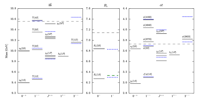
Figure 3: Results of our fit to $b\bar{b}$ and $c\bar{c}$ low-mass states, are shown by dotted blue lines on the background of data for heavy quarkonia and $B_{c}$ mesons. The dashed green line represents an average of various predictions for $B_{c}^{*}$ mass Gomez-Rocha:2016cji . Dashed lines across a panel represent thresholds. We include the states $3S$ that appear at the level of observed states that are interpreted as $4S$. Such highly excited states may contain an important component with effective gluons, not properly accounted for by the perturbative calculation in our pilot study.

To most accurately describe masses of $J/\psi$, $\psi(2S)$ and $\chi_{c1}(1P)$, one needs

$$m_{c} = 1460\text{ MeV}\quad\text{and}\quad\lambda_{c\bar{c}}\,=\,1944\text{ MeV}\ ,$$ (79)

and these values are associated with $\alpha(\lambda_{c\bar{c}})=0.3926$ and $\omega_{c\bar{c}}=321.6$ MeV. The resulting charmonium masses are illustrated in the right panel of Fig. 3.

Values of $\lambda_{b\bar{b}}$, $\lambda_{c\bar{c}}$, and $m_{b}$, $m_{c}$ fix

$$a = 1.589\ ,$$ (80)

$$b = 783\text{ MeV}\ .$$ (81)

These coefficients imply, according to Eq. (76),

$$\lambda_{bc} = 3134\text{ MeV}\ .$$ (82)

The middle panel of Fig. 3 shows the comparison of experimental masses of $B_{c}$ and $B_{c}(2S)$ and an average of different predictions for a mass of $B_{c}^{*}$ with our theoretical levels. Note that because we fit the masses of spin-one quarkonia while we neglect spin-dependent interactions, we present our mass estimates as for $1^{-}$. Because there are no experimental data to compare for spin-one $B_{c}^{*}$, we provide an average of various theoretical predictions Gomez-Rocha:2016cji . The agreement is satisfactory, given that we do not expect our estimates to be precise. Equation (82) gives

$$\alpha(\lambda_{bc}) = 0.3047\ ,$$ (83)

$$\omega_{bc} = 261.1\text{ MeV}\ .$$ (84)

7.3 Estimates of masses of heavy baryons

The fit to quarkonia described in Sec. 7.2 establishes optimal values of $\lambda$ for all baryons. Values of the coupling constant are obtained from Eq. (75). The optimal values we obtain for these parameters are listed in B. The resulting masses of heavy baryons are shown in Fig. 4. Labels of states describe internal orbital motion of quarks, where the first part of a label corresponds to the motion of quark $1$ with respect to quark $2$ and the second part corresponds to the motion of quark $3$ with respect to the pair of quarks $1$ and $2$. For example, in the state $1P1S$, the pair $12$ is in a $p$-wave without radial excitation, while the quark $3$ in its motion with respect to the pair $12$ is in an $s$-wave state without radial excitation. In $1S2S$, both $1$ with respect to $2$ and $3$ with respect to $12$ are in an $s$-wave state but the latter is radially excited. States $A$, $B$, $C$ and $D$ in $ccc$ and $bbb$ correspond to the second excitation of harmonic oscillator with excitation energy $2\omega$ above the ground state ($\omega\equiv\omega_{\text{baryon}}$). These states have spin-momentum wave functions that are symmetrized in a way due for fermions in colorless states. Details of the harmonic oscillator basis wave functions are described in D. Analytical formulas for masses of baryons are given in E.

The values of masses we obtain for $bbb$ and $ccc$ baryons agree well with model calculations Bjorken:1985ei ; Tsuge:1985ei ; SilvestreBrac:1996bg ; Jia:2006gw ; Martynenko:2007je ; Roberts:2007ni ; Vijande:2015faa including quark-diquark Giannuzzi:2009gh and hypercentral approximations Ghalenovi:2014swa ; Shah:2017jkr , bag models Ponce:1978gk ; Hasenfratz:1980ka ; Bernotas:2008bu , Regge phenomenology Wei:2015gsa ; Wei:2016jyk , sum rules Zhang:2009re ; Wang:2011ae ; Aliev:2012tt ; Aliev:2014lxa , pNRQCD LlanesEstrada:2011kc , Dyson-Schwinger approach SanchisAlepuz:2011aa ; Qin:2018dqp and lattice studies Brown:2014ena ; Meinel:2012qz ; Briceno:2012wt ; Padmanath:2013zfa ; Namekawa:2013vu ; Alexandrou:2014sha ; Can:2015exa , where comparison is available. As an example of comparison, we note that the ground state of $ccc$ is assigned masses from 4733 MeV to 4796 MeV, by different lattice calculations, with an average of 4768 MeV. Our result is 4797 MeV, differing by 29 MeV, or 0.6 % from the average. For $bbb$, the average of two lattice results we have identified is 14369 MeV, and our result is 14346 MeV, which is 23 MeV difference, or 0.2 %. These comparisons refer to Table I in Ref. Shah:2017jkr that summarizes results of calculations of masses of $\Omega_{ccc}$ and $\Omega_{bbb}$ reported in twenty different articles. Ground state of $bbc$ is also very close to the lattice result Brown:2014ena . In contrast, our $ccb$ differs by about 300 MeV from the lattice. We comment on this feature below. Comparison with lattice calculations reported in Ref. Meinel:2012qz shows that our splittings in $bbb$ differ only by about 10 %. In case of $ccc$ Padmanath:2013zfa , the difference of splittings does not exceed 20 %. This degree of agreement is surprising in view of the complexity of lattice calculations in comparison with the simplicity of our effective Hamiltonian calculation.

The prominent feature visible in Fig. 4 is the extraordinary magnitude of splittings in the $ccb$ baryons. It is a consequence of large oscillator frequency in $cc$ subsystem in Eq. (68), due to large ratio of $\lambda_{ccb}/m_{c}$, in which the scale parameter $\lambda_{ccb}$ is large in comparison with $m_{c}$ due to $m_{b}$. This separation of scales may make precise calculations of masses of excited $ccb$ baryons difficult. Since the harmonic excitation is so high, it is likely that components with gluons of mass on the order of 1 GeV have to be included in a nonperturbative way.

The surprising feature that the very crude, first approximation based on the RGPEP, with no free parameters left after adjusting quark masses and scale to $b\bar{b}$ and $c\bar{c}$ data, produces in an elementary analytic way similar splittings to the ones resulting from advanced calculations, is further illustrated in Fig. 5. It presents splittings in a second band of harmonic oscillator caused by Coulomb interactions. Splittings $m_{D}-m_{C}$, $m_{C}-m_{B}$, $m_{B}-m_{A}$ are in relation 2:1:5, which is the general result in the first order of perturbation theory for harmonic oscillator perturbed by any potential Isgur:1978wd .

Interestingly, analogous lattice QCD splittings with spin dependent interactions turned off Meinel:2012qz , also appear in the ratios 2:1:5. These results suggest that the RGPEP constituent picture with a gluon mass ansatz may be grasping the physics of lowest-mass heavy baryons. Since experimentally triply heavy baryons are difficult to produce and detect Olsen:2017bmm , their theoretical understanding using standard techniques is weakly motivated and hence also limited Brambilla:2010cs ; Brambilla:2014jmp . Therefore, the ease with which our method yields results for heavy baryons in agreement with complex approaches suggests that application of the RGPEP in fourth order and including components with one or more effective gluons in the eigenvalue problem beyond perturbation theory, are worth attempting.

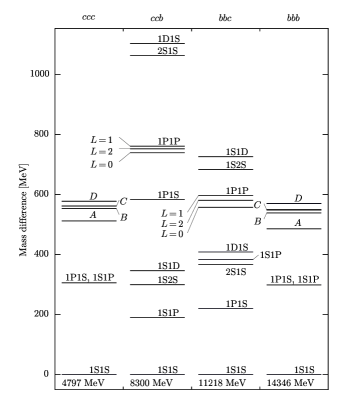
Figure 4: Qualitative picture of triply heavy baryon mass spectrum implied by the second-order RGPEP in heavy-flavor QCD and our gluon mass ansatz. The figure shows excitations above the ground states $1S1S$, whose absolute masses are written at the bottom of each column. The $ccb$ spectrum displays extraordinarily large mass excitation for states $1P1S$, $2S1S$ and $1D1S$ in $ccb$. Such high excitations are associated with formation of $cc$-diquarks, bound by a harmonic force that is strong because the charmed quarks are much lighter than the bottom quarks. Much less pronounced splittings appear in the $bbc$ baryons. See the text for further discussion.

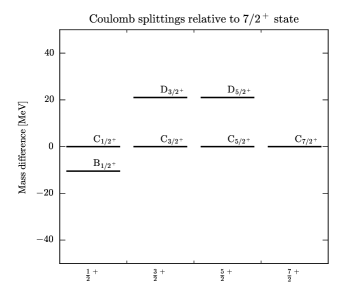
Figure 5: Expanded view of $B$, $C$ and $D$ states of $bbb$ in Fig. 4. The harmonic oscillator and Coulomb potential are sufficient to qualitatively reproduce the pattern of splittings presented in Fig. 11 in Ref. Meinel:2012qz . However, quantitatively our pilot-study splittings are about twice smaller. Precise agreement is not expected because our approximation is very crude and does not include spin interactions. Hence, it cannot match splittings between the $C$ states and between the $D$ states obtained in other calculations that include spin effects.

8 Conclusion

The effective Hamiltonians we finesse for heavy quarkonia and baryons from QCD of charm and beauty quarks using our gluon mass ansatz, lead to the baryon mass spectra in the ball park of expectations from other approaches to physics of $ccc$ and $bbb$ systems. In addition, the Hamiltonians suggest that quarks $c$ form tight diquarks in $ccb$ baryons. Diquarks are less likely in $bbc$ baryons. Other approaches do not foresee tight diquarks in $ccb$ baryons. This feature may thus distinguish a physically proper approach in future. However, such tight diquarks are hard to excite and mass splittings due their excitation are comparable or even exceed values of the gluon mass one may expect in theory. In that case, the highly excited baryon component with a heavy gluon may be large and our approximation to the three-quark component as dominant may be invalid. Calculations that treat the highly excited baryons as having significant components with one heavy effective gluon may yield smaller masses than our approximation based on the dominance of the three-quark component. If it were the case, the RGPEP approach would still apply, but in the domain of hadron physics in which gluons appear as constituents in competition with quarks for probability of appearance.

Taking into account that the method of RGPEP that we use is invariant under boosts and that it is a priori capable of providing a relativistic theory of hadrons in terms of a limited number of their effective constituents with suitably adjusted size, an extension of the RGPEP calculation to fourth order appears worth undertaking. It is certainly needed for verifying if the gluon mass ansatz we introduced provides an adequate representation of dynamics of gluons in the presence of heavy color sources. Fourth-order Hamiltonian is also needed for control on the spin splittings and rotational symmetry.

The ratio $\sqrt{8/6}$ of harmonic oscillator frequencies in heavy quarkonia and triply heavy baryons is close to the ratio $\sqrt{8/5}$ obtained for $u$ and $d$ constituent quarks in models using the concept of gluon condensate. If this is not accidental, one may hope that the RGPEP formalism shall apply also to light hadrons as built from constituent quarks and massive gluons, the latter nearly decoupled after generating effective interactions for quarks on the way down in $\lambda$ toward 1/fm GlazekWilson1998 ; GlazekMlynikAF . But even for heavy baryons alone, the effective oscillator picture provides simple wave functions that can be used in description of relativistic processes that involve heavy hadrons.

Appendix A Fits to masses of well-established quarkonia

Once the coupling constant $\alpha$ as a function of $\lambda$ is set, the eigenvalues of Eq. (73) estimated by evaluating expectation values of the Coulomb terms in known eigenstates of the oscillator part of the effective Hamiltonian,

$$E_{1S} = \frac{3}{2}\omega-\frac{4}{3}\alpha\sqrt{\frac{2}{\pi\nu}}\ ,$$ (85)

$$E_{2S} = \frac{7}{2}\omega-\frac{10}{9}\alpha\sqrt{\frac{2}{\pi\nu}}\ ,$$ (86)

$$E_{1P} = \frac{5}{2}\omega-\frac{8}{9}\alpha\sqrt{\frac{2}{\pi\nu}}\ ,$$ (87)

with

$$\omega = \sqrt{\frac{\alpha(\lambda_{Q\bar{Q}})}{18\sqrt{2\pi}}}\frac{\lambda_{Q\bar{Q}}^{3}}{m^{2}}\ ,\quad\quad\nu\,=\,\frac{1}{m\omega}\ ,$$ (88)

and $m=m_{c}$ or $m=m_{b}$, are used to evaluate corresponding masses from the formula

$$M = 2m\sqrt{1+\frac{E}{m}}\ .$$ (89)

These are compared with data PDG2016 . Thus, $\Upsilon(1S)$, $\Upsilon(2S)$ and $\chi_{b1}(1P)$ are used to find best values $m_{b}$ and $\lambda_{b\bar{b}}$, using $\chi^{2}$. We obtain,

$$m_{b} = 4698\text{ MeV}\ ,\quad\quad\lambda_{b\bar{b}}\,=\,4258\text{ MeV}\ .$$ (90)

Using $\alpha(\lambda_{b\bar{b}})=0.2664$, we find that $\omega_{b\bar{b}}=268.8$ MeV. Mean squared deviation (MSD) of the $b\bar{b}$ fit is $33$ MeV. Allowing for bigger MSD up to, say $50$ MeV, produces a set of acceptable values of $\lambda$ and $m_{b}$, illustrated in Fig. 6.

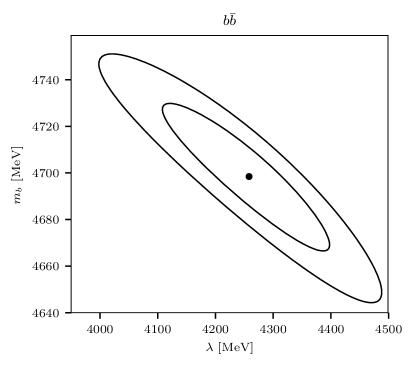
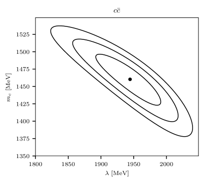
Figure 6: Contour plots of the square root of mean squared deviation of the fit on $\lambda$-$m$ plane for bottomonium and charmonium. The plotted contours correspond to $30$ (for charmonium only), $40$ and $50$ MeV. Dots indicate best fits.

For charmonia, $J/\psi$, $\psi(2S)$ and $\chi_{c1}(1P)$ masses are used in the same way to find best values of $m_{c}$ and $\lambda_{c\bar{c}}$, which turn out to be

$$m_{c} = 1460\text{ MeV}\ ,\quad\quad\lambda_{c\bar{c}}\,=\,1944\text{ MeV}\ .$$ (91)

Using $\alpha(\lambda_{c\bar{c}})=0.3926$, we obtain $\omega_{c\bar{c}}=321.6$ MeV. The MSD of the $c\bar{c}$ fit is $22$ MeV, see Fig. 6 for uncertainty of the fit. It is visible in Fig. 6 that there exist functions $m_{b}(\lambda)$ and $m_{c}(\lambda)$ that one might introduce to obtain some window of stability of the fit accuracy, exceeding 10% variation in $\lambda$. However, the pilot study appears too crude to us to believe that this stability already reflects the true behavior of quark masses in the theory, even though stability windows of that size naturally appear at order $\alpha$ in Hamiltonian matrix models with asymptotic freedom and bound states GlazekWilson1998 .

Two heavy mesons made of quarks $b$ and $c$ were observed, $B_{c}$ and $B_{c}(2S)$ PDG2016 . Fits to quarkonia fix masses of quarks, hence, the only free parameter is $\lambda_{bc}$, which we fix by assuming Eq. (76). Without any freedom left we plot in Fig. 3 the spectrum of $B_{c}$ using the same Eqs. (85) and (86), but with

$$\omega^{2} = \frac{\alpha(\lambda_{bc})}{18\sqrt{\pi}\,\mu_{bc}}\left(\frac{\lambda_{bc}^{2}}{\sqrt{m_{b}^{2}+m_{c}^{2}}}\right)^{3}\ ,$$ (92)

$$\nu = \frac{1}{2\mu_{bc}\omega}\ ,$$ (93)

$$\mu_{bc} = \frac{m_{b}m_{c}}{m_{b}+m_{c}}\ .$$ (94)

The physical quarkonia masses are read from

$$M = \left(m_{b}+m_{c}\right)\sqrt{1+\frac{2E}{m_{b}+m_{c}}}\ .$$ (95)

Appendix B Parameters for heavy baryons

We choose parameter $\lambda$ for a baryon system by assuming Eq. (77) where $a$ and $b$ are given in Eqs. (80) and (81). Values of $\lambda$ are solutions to the following equations

$$\lambda_{bbb} = \sqrt{\alpha(\lambda_{bbb})}\ \left(a\,m_{b}+b\right)\ ,$$ (96)

$$\lambda_{bbc} = \sqrt{\alpha(\lambda_{bbc})}\ \left(a\,\frac{2m_{b}+m_{c}}{3}+b\right)\ ,$$ (97)

$$\lambda_{ccb} = \sqrt{\alpha(\lambda_{ccb})}\ \left(a\,\frac{m_{b}+2m_{c}}{3}+b\right)\ ,$$ (98)

$$\lambda_{ccc} = \sqrt{\alpha(\lambda_{ccc})}\ \left(a\,m_{c}+b\right)\ .$$ (99)

We obtain:

$$\lambda_{bbb}\,=\,4258\text{ MeV}\ ,\quad\alpha(\lambda_{bbb})\,=\,0.2664\ ,$$ (100)

$$\lambda_{bbc}\,=\,3514\text{ MeV}\ ,\quad\alpha(\lambda_{bbc})\,=\,0.2892\ ,$$ (101)

$$\lambda_{ccb}\,=\,2746\text{ MeV}\ ,\quad\alpha(\lambda_{ccb})\,=\,0.3248\ ,$$ (102)

$$\lambda_{ccc}\,=\,1944\text{ MeV}\ ,\quad\alpha(\lambda_{ccc})\,=\,0.3926\ .$$ (103)

For readers’ convenience, we also listed above the associated values of coupling constant.

Appendix C Frequency diagram

Harmonic oscillator frequencies, Eqs. (68) and (69), depend on quark masses and on the scale $\lambda$. Figure 7 shows the dependence of $\omega_{12}$ and $\omega_{3(12)}$ on $\lambda$ for four different choices of three quark masses that correspond to the systems $bbb$, $bbc$, $ccb$ and $ccc$. For $ccc$ and $bbb$ we have $\omega_{12}=\omega_{3(12)}=\omega$. Blue vertical lines indicate the values of $\lambda$s for baryons from Eqs. (100) to (103). They end on a higher of two blue dots. The dots show the values of $\omega_{12}(\lambda)$ and $\omega_{3(12)}(\lambda)$ for a given system and for $\lambda$ adjusted to that system. The frequencies are,

$$\omega_{bbb} =232.8\text{ MeV,}$$ (104)

$$\omega_{12,\,bbc} =166.2\text{ MeV,}\quad\omega_{3(12),\,bbc}=336.7\text{ MeV,}$$ (105)

$$\omega_{12,\,ccb} =593.5\text{ MeV,}\quad\omega_{3(12),\,ccb}=142.7\text{ MeV,}$$ (106)

$$\omega_{ccc} =278.5\text{ MeV.}$$ (107)

On Fig. 7, there are also two green triangles at the bottom of the plot. They indicate the values of $m_{b}$ and $m_{c}$. Furthermore, Figure 7 presents also $\alpha(\lambda)$ given in Eq. (75) with a decreasing black line. Red vertical line shows the asymptote of $\alpha(\lambda)$ curve at $\lambda=\Lambda_{QCD}$.

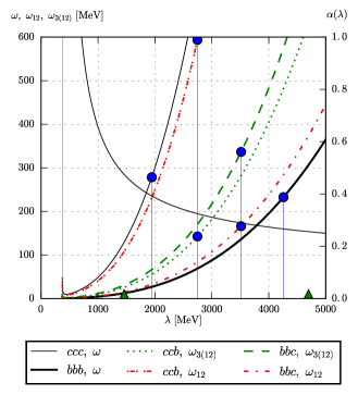
Figure 7: Dependence of the harmonic-oscillator frequencies on the RGPEP scale $\lambda$ and quark masses (left axis), and the dependence of $\alpha$ on $\lambda$ (right axis). For detailed description of this figure content, see C.

Appendix D Wave functions for baryons

The unperturbed harmonic oscillator basis for baryons is constructed from products of wave functions of two harmonic oscillators associated with relative motion of particles $1$ and $2$ (with momentum $\vec{K}_{12}$), and relative motion of particle $3$ of momentum $\vec{Q}_{3}$ with respect to the pair $12$.

Eigenfunctions for relative motion of two particles with reduced mass $\mu$ interacting with harmonic oscillator force characterized by frequency $\omega$ are

$$\psi_{klm}(p,\theta,\phi)=N_{kl}\ e^{-\nu p^{2}}\ L_{k}^{(l+1/2)}(2\nu p^{2})\ p^{l}Y_{lm}(\theta,\phi)\ ,$$ (108)

where $\nu=1/(2\mu\omega)$, $k$ is the radial excitation number, $l$ is the orbital angular momentum number of the state, $m$ is the projection of angular momentum on the $z$ axis, $Y_{lm}$ are spherical harmonics PDG2016 and $L_{k}^{a}(x)$ are generalized Laguerre polynomials. The first two polynomials are $L_{0}^{a}(x)=1$, $L_{1}^{a}(x)=1+a-x$. The normalization factors are

$$N_{kl} = \sqrt{\sqrt{\frac{2\nu^{3}}{\pi}}\frac{2^{k+2l+3}k!\nu^{l}}{(2k+2l+1)!!}}(2\pi)^{3/2}\ ,$$ (109)

so that $\int\frac{d^{3}p}{(2\pi)^{3}}\psi_{klm}^{*}\psi_{k^{\prime}l^{\prime}m^{\prime}}=\delta_{kk^{\prime}}\delta_{ll^{\prime}}\delta_{mm^{\prime}}\ .$ Finally, the energies are

$$E = \omega\left(2k+l+\frac{3}{2}\right)\ .$$ (110)

We use a convenient notation for products of wave functions of two harmonic oscillators,

$${\left|{(k_{12}+1)(l_{12})_{m_{12}}(k_{3(12)}+1)(l_{3(12)})_{m_{3(12)}}}\right\rangle}={\left|{\psi_{k_{12}l_{12}m_{12}}}\right\rangle}{\left|{\psi_{k_{3(12)}l_{3(12)}m_{3(12)}}}\right\rangle}\ ,$$ (111)

where index $12$ corresponds to harmonic oscillator between $1$ and $2$, with $\nu_{12}=1/(2\mu_{12}\omega_{12})$, and index $3(12)$ corresponds to harmonic oscillator between $3$ and $12$, with $\nu_{3(12)}=1/(2\mu_{3(12)}\omega_{3(12)})$. For example, the ground state is ${\left|{1S_{0}1S_{0}}\right\rangle}\equiv{\left|{1S1S}\right\rangle}$, while ${\left|{1P_{1}2S_{0}}\right\rangle}\equiv{\left|{1P_{1}2S}\right\rangle}$ is the state with harmonic oscillator between $1$ and $2$ excited to the first orbital excitation with angular momentum projection on $z$-axis equal $1$ and the harmonic oscillator between $3$ and $12$ being radially excited. The quantum numbers $m_{12}$ and $m_{3(12)}$ are omitted below, unless they are relevant.

We consider states whose excitation energies are at most $2\omega_{12}$ or $2\omega_{3(12)}$ or $\omega_{12}+\omega_{3(12)}$. That is, we consider states $1S1S$, $1P1S$, $1S1P$, $2S1S$, $1S2S$, $1D1S$, $1S1D$ and $1P1P$. The total angular momentum of a baryon is conserved, therefore, each state of the basis should have definite orbital angular momentum $L$. Since states ${\left|{1P_{m_{12}}1P_{m_{3(12)}}}\right\rangle}$ do not have definite angular momentum, we introduce instead the following states with angular momenta $L=2,1$ and $0$, respectively,

$${\left|{2,+2}\right\rangle} ={\left|{1P_{1}1P_{1}}\right\rangle}\ ,\quad{\left|{2,+1}\right\rangle}=\dots$$ (112)

$${\left|{1,+1}\right\rangle} =\frac{1}{\sqrt{2}}{\left|{1P_{1}1P_{0}}\right\rangle}-\frac{1}{\sqrt{2}}{\left|{1P_{0}1P_{1}}\right\rangle}\ ,\quad{\left|{1,0}\right\rangle}=\dots$$ (113)

$${\left|{0,\phantom{+}0}\right\rangle} =\frac{1}{\sqrt{3}}\left(\phantom{\frac{}{}}{\left|{1P_{1}1P_{-1}}\right\rangle}-{\left|{1P_{0}1P_{0}}\right\rangle}+{\left|{1P_{-1}1P_{1}}\right\rangle}\phantom{\frac{}{}}\right)\ ,$$ (114)

where only the highest $L_{z}$ state is written explicitly. The construction of these states is done in accordance with the rules of adding angular momenta in quantum mechanics and we use convention defined in PDG2016 in the tables of Clebsch-Gordan coefficients.

Because quarks have spin, we also need to construct the spin wave functions. We define spin-$3/2$ quadruplet, which is fully symmetric with respect to exchange of any pair of quarks,

$${\left|{+\frac{3}{2}}\right\rangle} = {\left|{{\uparrow}{\uparrow}{\uparrow}}\right\rangle}\ ,\quad{\left|{+\frac{1}{2}}\right\rangle}\,=\,\dots\ ;$$ (115)

spin-$1/2$ doublet, which we call $(1/2)_{S}$ and which is $12$-symmetric,

$${\left|{+\frac{1}{2}S}\right\rangle} = \sqrt{\frac{2}{3}}\left(\phantom{+}{\left|{{\uparrow}{\uparrow}{\downarrow}}\right\rangle}-\frac{1}{2}{\left|{{\uparrow}{\downarrow}{\uparrow}}\right\rangle}-\frac{1}{2}{\left|{{\downarrow}{\uparrow}{\uparrow}}\right\rangle}\right)\ ,$$ (116)

$${\left|{-\frac{1}{2}S}\right\rangle} = \sqrt{\frac{2}{3}}\left(-{\left|{{\downarrow}{\downarrow}{\uparrow}}\right\rangle}+\frac{1}{2}{\left|{{\downarrow}{\uparrow}{\downarrow}}\right\rangle}+\frac{1}{2}{\left|{{\uparrow}{\downarrow}{\downarrow}}\right\rangle}\right)\ ;$$ (117)

and another spin-$1/2$ doublet, which we call $(1/2)_{A}$ and which is $12$-antisymmetric,

$${\left|{+\frac{1}{2}A}\right\rangle} = \sqrt{\frac{1}{2}}\left({\left|{{\uparrow}{\downarrow}{\uparrow}}\right\rangle}-{\left|{{\downarrow}{\uparrow}{\uparrow}}\right\rangle}\right)\ ,$$ (118)

$${\left|{-\frac{1}{2}A}\right\rangle} = \sqrt{\frac{1}{2}}\left({\left|{{\uparrow}{\downarrow}{\downarrow}}\right\rangle}-{\left|{{\downarrow}{\uparrow}{\downarrow}}\right\rangle}\right)\ .$$ (119)

For completeness, we describe our construction of states of definite total angular momentum. First consider $ccb$ and $bbc$ systems, where quarks $1$ and $2$ are identical and $3$ is different. Because quarks $1$ and $2$ are identical, the total spin-momentum wave function has to be $12$-symmetric; color-singlet wave function is antisymmetric. Therefore, one must add orbital angular momentum and spin respecting the Pauli exclusion principle for fermions. For example, the states ${\left|{1P1S}\right\rangle}$ are $12$-antisymmetric and to obtain $12$-symmetric spin-momentum wave function we can combine them only with spin $(1/2)_{A}$, which is also $12$-antisymmetric. States ${\left|{1S1P}\right\rangle}$ are $12$-symmetric and we can combine them only with spin $3/2$ and $(1/2)_{S}$. The list of possible states is summarized in Table 1.

Table 1: Summary of oscillator basis states for systems $ccb$ and $bbc$.

States	$L\otimes S$	J
1S1S	$0\otimes\frac{3}{2}$	${\frac{3}{2}}^{+}$
	$0\otimes\left(\frac{1}{2}\right)_{S}$	${\frac{1}{2}}^{+}$
1P1S	$1\otimes\left(\frac{1}{2}\right)_{A}$	${\frac{3}{2}}^{-}\oplus{\frac{1}{2}}^{-}$
1S1P	$1\otimes\frac{3}{2}$	${\frac{5}{2}}^{-}\oplus{\frac{3}{2}}^{-}\oplus{\frac{1}{2}}^{-}$
	$1\otimes\left(\frac{1}{2}\right)_{S}$	${\frac{3}{2}}^{-}\oplus{\frac{1}{2}}^{-}$
1D1S	$2\otimes\frac{3}{2}$	${\frac{7}{2}}^{+}\oplus{\frac{5}{2}}^{+}\oplus{\frac{3}{2}}^{+}\oplus{\frac{1}{2}}^{+}$
	$2\otimes\left(\frac{1}{2}\right)_{S}$	${\frac{5}{2}}^{+}\oplus{\frac{3}{2}}^{+}$
1S1D	$2\otimes\frac{3}{2}$	${\frac{7}{2}}^{+}\oplus{\frac{5}{2}}^{+}\oplus{\frac{3}{2}}^{+}\oplus{\frac{1}{2}}^{+}$
	$2\otimes\left(\frac{1}{2}\right)_{S}$	${\frac{5}{2}}^{+}\oplus{\frac{3}{2}}^{+}$
1P1P	$2\otimes\left(\frac{1}{2}\right)_{A}$	${\frac{5}{2}}^{+}\oplus{\frac{3}{2}}^{+}$
	$1\otimes\left(\frac{1}{2}\right)_{A}$	${\frac{3}{2}}^{+}\oplus{\frac{1}{2}}^{+}$
	$0\otimes\left(\frac{1}{2}\right)_{A}$	${\frac{1}{2}}^{+}$

To obtain the explicit formulas for the wave functions, we use Clebsch-Gordan tables, as in Eqs. (112) to (114).

D.1 Symmetric wave functions

In the case of three identical quarks, we need to use fully symmetric wave functions. One can symmetrize the wave functions given above. The ground state $1S1S$ wave function is fully symmetric in momentum, and we can combine it only with spin $3/2$. By the way, symmetrization of $1S1S$ with $(1/2)_{S}$ gives zero. In this case the wave function is the same as in the case of only two quarks being identical,

$${\left|{0\omega,\frac{3}{2}^{+},J_{z}}\right\rangle} = {\left|{1S1S}\right\rangle}{\left|{J_{z}}\right\rangle}\ ,$$ (120)

where $J_{z}=+3/2,+1/2,-1/2,-3/2$ is the projection of baryon spin on $z$-axis.

After symmetrization of the oscillator once-excited states $1P1S$ and $1S1P$, one is left with only two linearly independent multiplets of states, whose wave functions are (we write only the highest $J_{z}$ state in each multiplet, more information is available in Table 2)

$${\left|{1\omega,\frac{3}{2}^{-},+\frac{3}{2}}\right\rangle} = \frac{1}{\sqrt{2}}{\left|{1P_{1}1S}\right\rangle}{\left|{+\frac{1}{2}A}\right\rangle}-\frac{1}{\sqrt{2}}{\left|{1S1P_{1}}\right\rangle}{\left|{+\frac{1}{2}S}\right\rangle}\ ,$$ (121)

$${\left|{1\omega,\frac{1}{2}^{-},+\frac{1}{2}}\right\rangle} = -\frac{1}{\sqrt{6}}{\left|{1P_{0}1S}\right\rangle}{\left|{+\frac{1}{2}A}\right\rangle}+\frac{1}{\sqrt{3}}{\left|{1P_{1}1S}\right\rangle}{\left|{-\frac{1}{2}A}\right\rangle}$$ (122)

$$+ \frac{1}{\sqrt{6}}{\left|{1S1P_{0}}\right\rangle}{\left|{+\frac{1}{2}S}\right\rangle}-\frac{1}{\sqrt{3}}{\left|{1S1P_{1}}\right\rangle}{\left|{-\frac{1}{2}S}\right\rangle}\ .$$

The symmetrization of a band of twice-excited oscillator states, $2S1S$, $1S2S$, $1D1S$, $1S1D$ and $1P1P$ reduces the number of linearly independent multiplets from 21 to 8 (compare Tables 1 and 2). Highest $J_{z}$ states in each multiplet are

$${\left|{A_{\frac{3}{2}^{+}},+\frac{3}{2}}\right\rangle} = {\left|{2S1S}\right\rangle}_{+}{\left|{+\frac{3}{2}}\right\rangle}\ ,$$ (123)

$${\left|{B_{\frac{1}{2}^{+}},+\frac{1}{2}}\right\rangle} = \frac{1}{\sqrt{2}}{\left|{2S1S}\right\rangle}_{-}{\left|{+\frac{1}{2}S}\right\rangle}-\frac{1}{\sqrt{2}}{\left|{0,0}\right\rangle}{\left|{+\frac{1}{2}A}\right\rangle}\ ,$$ (124)

$${\left|{C_{\frac{7}{2}^{+}},+\frac{7}{2}}\right\rangle} = {\left|{1D_{2}1S}\right\rangle}_{+}{\left|{+\frac{3}{2}}\right\rangle}\ ,$$ (125)

$${\left|{C_{\frac{5}{2}^{+}},+\frac{5}{2}}\right\rangle} = -\sqrt{\frac{3}{7}}{\left|{1D_{1}1S}\right\rangle}_{+}{\left|{+\frac{3}{2}}\right\rangle}+\sqrt{\frac{4}{7}}{\left|{1D_{2}1S}\right\rangle}_{+}{\left|{+\frac{1}{2}}\right\rangle}\ ,$$ (126)

$${\left|{C_{\frac{3}{2}^{+}},+\frac{3}{2}}\right\rangle} = \sqrt{\frac{1}{5}}{\left|{1D_{0}1S}\right\rangle}_{+}{\left|{+\frac{3}{2}}\right\rangle}-\sqrt{\frac{2}{5}}{\left|{1D_{1}1S}\right\rangle}_{+}{\left|{+\frac{1}{2}}\right\rangle}+\sqrt{\frac{2}{5}}{\left|{1D_{2}1S}\right\rangle}_{+}{\left|{-\frac{1}{2}}\right\rangle}\ ,$$

$${\left|{C_{\frac{1}{2}^{+}},+\frac{1}{2}}\right\rangle} = -\sqrt{\frac{1}{10}}{\left|{1D_{-1}1S}\right\rangle}_{+}{\left|{+\frac{3}{2}}\right\rangle}+\sqrt{\frac{1}{5}}{\left|{1D_{0}1S}\right\rangle}_{+}{\left|{+\frac{1}{2}}\right\rangle}$$ (128)

$$- \sqrt{\frac{3}{10}}{\left|{1D_{1}1S}\right\rangle}_{+}{\left|{-\frac{1}{2}}\right\rangle}+\sqrt{\frac{2}{5}}{\left|{1D_{2}1S}\right\rangle}_{+}{\left|{-\frac{3}{2}}\right\rangle}\ ,$$

$${\left|{D_{\frac{5}{2}^{+}},+\frac{5}{2}}\right\rangle} = \frac{1}{\sqrt{2}}{\left|{1D_{2}1S}\right\rangle}_{-}{\left|{+\frac{1}{2}S}\right\rangle}-\frac{1}{\sqrt{2}}{\left|{2,+2}\right\rangle}{\left|{+\frac{1}{2}A}\right\rangle}\ ,$$ (129)

$${\left|{D_{\frac{3}{2}^{+}},+\frac{3}{2}}\right\rangle} = -\sqrt{\frac{1}{10}}{\left|{1D_{1}1S}\right\rangle}_{-}{\left|{+\frac{1}{2}S}\right\rangle}+\sqrt{\frac{2}{5}}{\left|{1D_{2}1S}\right\rangle}_{-}{\left|{-\frac{1}{2}S}\right\rangle}$$ (130)

$$+ \sqrt{\frac{1}{10}}{\left|{2,+1}\right\rangle}{\left|{+\frac{1}{2}A}\right\rangle}-\sqrt{\frac{2}{5}}{\left|{2,+2}\right\rangle}{\left|{-\frac{1}{2}A}\right\rangle}\ ,$$

where

$${\left|{2S1S}\right\rangle}_{\pm} = \frac{{\left|{2S1S}\right\rangle}\pm{\left|{1S2S}\right\rangle}}{\sqrt{2}}\ ,$$ (131)

$${\left|{1D_{m}1S}\right\rangle}_{\pm} = \frac{{\left|{1D_{m}1S}\right\rangle}\pm{\left|{1S1D_{m}}\right\rangle}}{\sqrt{2}}\ .$$ (132)

States with $J_{z}$ different than the highest $J_{z}$ available in the multiplet can be constructed according to Table 2.

Table 2: Summary of states for systems $ccc$ and $bbb$. For example, $1D1S_{-}\otimes\left(\frac{1}{2}\right)_{S}$ means that we use ${\left|{1D_{m}1S}\right\rangle}_{-}$ states and $(1/2)_{S}$ spin states to obtain one of $J=5/2$ or $J=3/2$ states according to the rules of adding angular momenta, i.e., using the Clebsch-Gordan coefficients. $1P1P_{L=2}\otimes\left(\frac{1}{2}\right)_{A}$ means that we take $L=2$ states, given in Eq. (112), and $(1/2)_{A}$ spin states to obtain a state with the same quantum numbers. We then subtract the latter from the former, as indicated in the table, and normalize the result to obtain the final expression, such as in Eqs. (129) or (130), where the states with $J=5/2$, $J_{z}=+5/2$ and $J=3/2$, $J_{z}=+3/2$ are written explicitly. Our prescription differs in sign from the prescriptions known in the literature Isgur:1978wd ; Capstick:2000qj , because our momentum $\vec{Q}_{3}$ is a momentum of quark $3$ with respect to pair $12$, instead of pair $12$ with respect to quark $3$.

States	Wave functions	Baryons
$0\omega$	$1S1S\otimes\frac{3}{2}$	${\frac{3}{2}}^{+}$
$1\omega$	$1P1S\otimes\left(\frac{1}{2}\right)_{A}-1S1P\otimes\left(\frac{1}{2}\right)_{S}$	${\frac{3}{2}}^{-}\oplus{\frac{1}{2}}^{-}$
A	$2S1S_{+}\otimes\frac{3}{2}$	${\frac{3}{2}}^{+}$
B	$2S1S_{-}\otimes\left(\frac{1}{2}\right)_{S}-1P1P_{L=0}\otimes\left(\frac{1}{2}\right)_{A}$	${\frac{1}{2}}^{+}$
C	$1D1S_{+}\otimes\frac{3}{2}$	${\frac{7}{2}}^{+}\oplus\dots\oplus{\frac{1}{2}}^{+}$
D	$1D1S_{-}\otimes\left(\frac{1}{2}\right)_{S}-1P1P_{L=2}\otimes\left(\frac{1}{2}\right)_{A}$	${\frac{5}{2}}^{+}\oplus{\frac{3}{2}}^{+}$

Appendix E Baryon masses

E.1 States $ccb$ and $bbc$

Baryon masses are given by Eq. (72), where

$$E = \omega_{12}\left(2k_{12}+l_{12}+\frac{3}{2}\right)+\omega_{3(12)}\left(2k_{3(12)}+l_{3(12)}+\frac{3}{2}\right)+V\ ,$$ (133)

and $V={\left\langle{\cdot}\right|}\,\hat{V}_{C}\,{\left|{\cdot}\right\rangle}$ is the expectation value of Coulomb interaction in the harmonic oscillator eigenstates. For example,

$$E_{1P1P}^{L=0} = \frac{5}{2}\omega_{12}+\frac{5}{2}\omega_{3(12)}+V_{1P1P}^{L=0}\ ,$$ (134)

where $V_{1P1P}^{L=0}={\left\langle{0,0}\right|}\,\hat{V}_{C}\,{\left|{0,0}\right\rangle}$. We define,

$$V = -\frac{2}{3}\alpha\sqrt{\frac{2}{\pi\nu_{12}}}\tilde{V}$$ (135)

and

$$x = \frac{4\nu_{3(12)}}{\nu_{12}}\ .$$ (136)

We list the Coulomb interaction expectation values for $ccb$ and $bbc$ states in Fig. 4.

$$\tilde{V}_{1S1S} = 1+\frac{4}{\sqrt{1+x}}\ ,$$ (137)

$$\tilde{V}_{1P1S} = \frac{2}{3}+\frac{4\left(3x+2\right)}{3(1+x)^{3/2}}\ ,$$ (138)

$$\tilde{V}_{1S1P} = 1+\frac{4(2x+3)}{3(1+x)^{3/2}}\ ,$$ (139)

$$\tilde{V}_{1P1P}^{L=0} = \frac{2}{3}+\frac{4(2x^{2}+7x+2)}{3(1+x)^{5/2}}\ ,$$ (140)

$$\tilde{V}_{1P1P}^{L=1} = \frac{2}{3}+\frac{8}{3\sqrt{x+1}}\ ,$$ (141)

$$\tilde{V}_{1P1P}^{L=2} = \frac{2}{3}+\frac{8\left(5x^{2}+13x+5\right)}{15(x+1)^{5/2}}\ ,$$ (142)

$$\tilde{V}_{1D1S} = \frac{8}{15}+\frac{4\left(15x^{2}+20x+8\right)}{15(1+x)^{5/2}}\ ,$$ (143)

$$\tilde{V}_{1S1D} = 1+\frac{4\left(8x^{2}+20x+15\right)}{15(1+x)^{5/2}}\ ,$$ (144)

$$\tilde{V}_{2S1S} = \frac{5}{6}+\frac{2\left(6x^{2}+8x+5\right)}{3(1+x)^{5/2}}\ ,$$ (145)

$$\tilde{V}_{1S2S} = 1+\frac{2\left(5x^{2}+8x+6\right)}{3(1+x)^{5/2}}\ .$$ (146)

E.2 States $ccc$ and $bbb$

For baryons $ccc$ and $bbb$, we also make use of Eqs. (133), (135) and (136). Formulas for ground states and once orbitally excited states do not change. For identical quarks $x=3$, and

$$\tilde{V}_{1S1S} = 3\ ,$$ (147)

$$\tilde{V}_{1\omega} = \frac{5}{2}\ .$$ (148)

Energies for states $A$, $B$, $C$ and $D$ need to be evaluated separately. We have

$$\tilde{V}_{A} = \frac{11}{4}\ ,$$ (149)

$$\tilde{V}_{B} = \frac{19}{8}\ ,$$ (150)

$$\tilde{V}_{C} = \frac{23}{10}\ ,$$ (151)

$$\tilde{V}_{D} = \frac{43}{20}\ .$$ (152)

References

- (1) S. Capstick, W. Roberts, Prog. Part. Nucl. Phys. 45, S241 (2000). DOI 10.1016/S0146-6410(00)00109-5
- (2) S. Capstick, N. Isgur, Phys. Rev. D34, 2809 (1986). DOI 10.1103/PhysRevD.34.2809
- (3) S.D. Głazek, M. Gómez-Rocha, J. More, K. Serafin, Phys. Lett. B773(9), 172 (2017). DOI 10.1016/j.physletb.2017.08.018
- (4) G. ’t Hooft, Nucl. Phys. B61, 455 (1973). DOI 10.1016/0550-3213(73)90376-3
- (5) K.G. Wilson, T.S. Walhout, A. Harindranath, W.M. Zhang, R.J. Perry, S.D. Glazek, Phys. Rev. D49, 6720 (1994). DOI 10.1103/PhysRevD.49.6720
- (6) G. Parisi, R. Petronzio, Phys. Lett. 94B, 51 (1980). DOI 10.1016/0370-2693(80)90822-9
- (7) J.M. Cornwall, Phys. Rev. D26, 1453 (1982). DOI 10.1103/PhysRevD.26.1453
- (8) A.C. Aguilar, D. Binosi, C.T. Figueiredo, J. Papavassiliou, Eur. Phys. J. C78(3), 181 (2018). DOI 10.1140/epjc/s10052-018-5679-2
- (9) C. Patrignani, et al., Chin. Phys. C40(10), 100001 (2016). DOI 10.1088/1674-1137/40/10/100001
- (10) E. Eichten, K. Gottfried, T. Kinoshita, K.D. Lane, T.M. Yan, Phys. Rev. D17, 3090 (1978). DOI 10.1103/PhysRevD.17.3090. [Erratum: Phys. Rev.D21,313(1980)]
- (11) S.D. Glazek, Acta Phys. Polon. B43, 1843 (2012). DOI 10.5506/APhysPolB.43.1843
- (12) C. Semay, B. Silvestre-Brac, Nucl. Phys. A618, 455 (1997). DOI 10.1016/S0375-9474(97)00060-2
- (13) K.J. Juge, J. Kuti, C. Morningstar, Phys. Rev. Lett. 90, 161601 (2003). DOI 10.1103/PhysRevLett.90.161601
- (14) T.T. Takahashi, H. Suganuma, Phys. Rev. Lett. 90, 182001 (2003). DOI 10.1103/PhysRevLett.90.182001
- (15) P.A.M. Dirac, Rev. Mod. Phys. 21, 392 (1949). DOI 10.1103/RevModPhys.21.392
- (16) G.P. Lepage, S.J. Brodsky, Phys. Rev. D22, 2157 (1980). DOI 10.1103/PhysRevD.22.2157
- (17) S.J. Brodsky, H.C. Pauli, S.S. Pinsky, Phys. Rept. 301, 299 (1998). DOI 10.1016/S0370-1573(97)00089-6
- (18) S.D. Glazek, K.G. Wilson, Phys. Rev. D48, 5863 (1993). DOI 10.1103/PhysRevD.48.5863
- (19) A. Casher, L. Susskind, Phys. Rev. D9, 436 (1974). DOI 10.1103/PhysRevD.9.436
- (20) P. Maris, C.D. Roberts, P.C. Tandy, Phys. Lett. B420, 267 (1998). DOI 10.1016/S0370-2693(97)01535-9
- (21) S.J. Brodsky, C.D. Roberts, R. Shrock, P.C. Tandy, Phys. Rev. C82, 022201 (2010). DOI 10.1103/PhysRevC.82.022201
- (22) S.D. Glazek, Acta Phys. Polon. B42, 1933 (2011). DOI 10.5506/APhysPolB.42.1933
- (23) S.J. Brodsky, C.D. Roberts, R. Shrock, P.C. Tandy, Phys. Rev. C85, 065202 (2012). DOI 10.1103/PhysRevC.85.065202
- (24) M. Gómez-Rocha, S.D. Głazek, Phys. Rev. D92(6), 065005 (2015). DOI 10.1103/PhysRevD.92.065005
- (25) K.G. Wilson, Phys. Rev. D2, 1438 (1970). DOI 10.1103/PhysRevD.2.1438
- (26) A.P. Trawiński, S.D. Głazek, S.J. Brodsky, G.F. de Téramond, H.G. Dosch, Phys. Rev. D90(7), 074017 (2014). DOI 10.1103/PhysRevD.90.074017
- (27) S.D. Głazek, M. Schaden, Phys. Lett. B198, 42 (1987). DOI 10.1016/0370-2693(87)90154-7
- (28) S.D. Glazek, K.G. Wilson, Phys. Rev. D57, 3558 (1998). DOI 10.1103/PhysRevD.57.3558
- (29) S.D. Glazek, J. Mlynik, Phys. Rev. D67, 045001 (2003). DOI 10.1103/PhysRevD.67.045001
- (30) M. Gómez-Rocha, T. Hilger, A. Krassnigg, Phys. Rev. D93(7), 074010 (2016). DOI 10.1103/PhysRevD.93.074010
- (31) J.D. Bjorken, AIP Conf. Proc. 132, 390 (1985). DOI 10.1063/1.35379
- (32) M. Tsuge, T. Morii, J. Morishita, Mod. Phys. Lett. A1, 131 (1986). DOI 10.1142/S0217732386000191. [Erratum: Mod. Phys. Lett.A2,283(1987)]
- (33) B. Silvestre-Brac, Few Body Syst. 20, 1 (1996). DOI 10.1007/s006010050028
- (34) Y. Jia, JHEP 10, 073 (2006). DOI 10.1088/1126-6708/2006/10/073
- (35) A.P. Martynenko, Phys. Lett. B663, 317 (2008). DOI 10.1016/j.physletb.2008.04.030
- (36) W. Roberts, M. Pervin, Int. J. Mod. Phys. A23, 2817 (2008). DOI 10.1142/S0217751X08041219
- (37) J. Vijande, A. Valcarce, H. Garcilazo, Phys. Rev. D91(5), 054011 (2015). DOI 10.1103/PhysRevD.91.054011
- (38) F. Giannuzzi, Phys. Rev. D79, 094002 (2009). DOI 10.1103/PhysRevD.79.094002
- (39) Z. Ghalenovi, A.A. Rajabi, S.x. Qin, D.H. Rischke, Mod. Phys. Lett. A29, 1450106 (2014). DOI 10.1142/S0217732314501065
- (40) Z. Shah, A.K. Rai, Eur. Phys. J. A53(10), 195 (2017). DOI 10.1140/epja/i2017-12386-2
- (41) W. Ponce, Phys. Rev. D19, 2197 (1979). DOI 10.1103/PhysRevD.19.2197
- (42) P. Hasenfratz, R.R. Horgan, J. Kuti, J.M. Richard, Phys. Lett. 94B, 401 (1980). DOI 10.1016/0370-2693(80)90906-5
- (43) A. Bernotas, V. Simonis, Lith. J. Phys. 49, 19 (2009). DOI 10.3952/lithjphys.49110
- (44) K.W. Wei, B. Chen, X.H. Guo, Phys. Rev. D92(7), 076008 (2015). DOI 10.1103/PhysRevD.92.076008
- (45) K.W. Wei, B. Chen, N. Liu, Q.Q. Wang, X.H. Guo, Phys. Rev. D95(11), 116005 (2017). DOI 10.1103/PhysRevD.95.116005
- (46) J.R. Zhang, M.Q. Huang, Phys. Lett. B674, 28 (2009). DOI 10.1016/j.physletb.2009.02.056
- (47) Z.G. Wang, Commun. Theor. Phys. 58, 723 (2012). DOI 10.1088/0253-6102/58/5/17
- (48) T.M. Aliev, K. Azizi, M. Savci, JHEP 04, 042 (2013). DOI 10.1007/JHEP04(2013)042
- (49) T.M. Aliev, K. Azizi, M. Savcı, J. Phys. G41, 065003 (2014). DOI 10.1088/0954-3899/41/6/065003
- (50) F.J. Llanes-Estrada, O.I. Pavlova, R. Williams, Eur. Phys. J. C72, 2019 (2012). DOI 10.1140/epjc/s10052-012-2019-9
- (51) H. Sanchis-Alepuz, R. Alkofer, G. Eichmann, R. Williams, PoS QCD-TNT-II, 041 (2011)
- (52) S.X. Qin, C.D. Roberts, S.M. Schmidt, Phys. Rev. D97(11), 114017 (2018). DOI 10.1103/PhysRevD.97.114017
- (53) Z.S. Brown, W. Detmold, S. Meinel, K. Orginos, Phys. Rev. D90(9), 094507 (2014). DOI 10.1103/PhysRevD.90.094507
- (54) S. Meinel, Phys. Rev. D85, 114510 (2012). DOI 10.1103/PhysRevD.85.114510
- (55) R.A. Briceno, H.W. Lin, D.R. Bolton, Phys. Rev. D86, 094504 (2012). DOI 10.1103/PhysRevD.86.094504
- (56) M. Padmanath, R.G. Edwards, N. Mathur, M. Peardon, Phys. Rev. D90(7), 074504 (2014). DOI 10.1103/PhysRevD.90.074504
- (57) Y. Namekawa, et al., Phys. Rev. D87(9), 094512 (2013). DOI 10.1103/PhysRevD.87.094512
- (58) C. Alexandrou, V. Drach, K. Jansen, C. Kallidonis, G. Koutsou, Phys. Rev. D90(7), 074501 (2014). DOI 10.1103/PhysRevD.90.074501
- (59) K.U. Can, G. Erkol, M. Oka, T.T. Takahashi, Phys. Rev. D92(11), 114515 (2015). DOI 10.1103/PhysRevD.92.114515
- (60) N. Isgur, G. Karl, Phys. Rev. D19, 2653 (1979). DOI 10.1103/PhysRevD.19.2653. [Erratum: Phys. Rev.D23,817(1981)]
- (61) S.L. Olsen, T. Skwarnicki, D. Zieminska, Rev. Mod. Phys. 90(1), 015003 (2018). DOI 10.1103/RevModPhys.90.015003
- (62) N. Brambilla, et al., Eur. Phys. J. C71, 1534 (2011). DOI 10.1140/epjc/s10052-010-1534-9
- (63) N. Brambilla, et al., Eur. Phys. J. C74(10), 2981 (2014). DOI 10.1140/epjc/s10052-014-2981-5