A Systematic Approach to Constructing Incremental Topology Control Algorithms Using Graph Transformation

Abstract

This document corresponds to the accepted manuscript of the article Kluge, R., Stein, M., Varró, G., Schürr, A., Hollick, M., Mühlhäuser, M.: ”A Systematic Approach to Constructing Incremental Topology Control Algorithms using Graph Transformation,” in: JVLC 2016. The URL of the formal version is https://dx.doi.org/10.1016/j.jvlc.2016.10.003. This document is made available under the CC-BY-NC-ND 4.0 license http://creativecommons.org/licenses/by-nc-nd/4.0/.

Communication networks form the backbone of our society. Topology control algorithms optimize the topology of such communication networks. Due to the importance of communication networks, a topology control algorithm should guarantee certain required consistency properties (e.g., connectivity of the topology), while achieving desired optimization properties (e.g., a bounded number of neighbors). Real-world topologies are dynamic (e.g., because nodes join, leave, or move within the network), which requires topology control algorithms to operate in an incremental way, i.e., based on the recently introduced modifications of a topology. Visual programming and specification languages are a proven means for specifying the structure as well as consistency and optimization properties of topologies. In this paper, we present a novel methodology, based on a visual graph transformation and graph constraint language, for developing incremental topology control algorithms that are guaranteed to fulfill a set of specified consistency and optimization constraints. More specifically, we model the possible modifications of a topology control algorithm and the environment using graph transformation rules, and we describe consistency and optimization properties using graph constraints. On this basis, we apply and extend a well-known constructive approach to derive refined graph transformation rules that preserve these graph constraints. We apply our methodology to re-engineer an established topology control algorithm, kTC, and evaluate it in a network simulation study to show the practical applicability of our approach.

1 Introduction

Topology control (TC) is an important research area in the wireless network communication domain. TC aims at adapting the topology of wireless networks to optimize, for instance, the total power consumption, while maintaining crucial constraints of the topology (e.g., connectivity) [1, 2, 3, 4, 5]. A TC algorithm typically works by (i) first selecting a subset of the links of the original topology so that all required constraints are fulfilled, and (ii) then adjusting the transmission power of each node to reach its farthest neighbor across one of these selected links. In realistic settings, context events such as movement of sensor nodes continuously modify the structure of a topology. Therefore, a TC algorithm should operate in an incremental way by efficiently updating only the affected subset of links based on the occurred context events.

The development of a TC algorithm is performed by highly skilled and experienced professionals. The development process usually starts with an informal specification of the basic properties of a TC algorithm. This informal description is then supplemented by a formal specification using a theoretically well-founded framework such as graph theory [6, 7, 8] or game theory [9, 10], which allows to prove that the algorithm preserves all required constraints. The first evaluation of a TC algorithm is typically carried out using a network simulator, which may be succeeded by a second evaluation in a testbed environment, i.e., on real wireless devices. Both types of evaluation require an implementation of the TC algorithm in one or—most often—two programming languages, such as Java or MATLAB for the simulation and C or C++ for the testbed evaluation [11]. This means that, in the end, the (hopefully) same TC algorithm is represented in two or three more or less completely different representations. In research publications, often only the formalization (along with the proofs of correctness and optimality) and a pseudo-code representation of the TC algorithm is given, while the implementations are typically omitted. Still, even for skilled researchers, it may be difficult to verify that the pseudo code is a valid implementation of the formal specification.

In the following, we illustrate this by means of the Cooperative Topology Control Algorithm (CTCA), proposed by Chu and Sethu in an IEEE INFOCOM paper in 2012 [12]. The authors first give a graph-based intuition of the proposed TC algorithm, which shall lead to an improved distribution of the nodes’ lifetimes in a wireless sensor network [12, Sec. III]. The resulting goals are then formalized as so-called ordinary potential game [13], which allows to prove that the proposed algorithm eventually leads to a stable and optimal state of the network. The authors present an implementation of their algorithm in pseudo code, which is 83 lines long, distributed across four listings, and enriched with network-specific aspects such as communication message exchange; all these aspects make it highly non-trivial to understand the correspondences to the game-theoretic formalization [12, Sec. V]. In a simulation-based evaluation, the authors compare CTCA with other state-of-the-art TC algorithms. Unfortunately, no details about the simulation platform are given [12, Sec. VI]. To the best of our knowledge, no testbed evaluation of CTCA has been performed yet.

While the previous example considers only one of the many existing TC algorithms, experience shows that it is (at least partly) representative. The example illustrates an obvious and prevalent gap between the formal specification, which serves for proving important properties of the algorithm, and the implementation, which serves for assessing the TC algorithm. Due to this gap, it inherently remains unclear whether the evaluated implementation of a TC algorithm fulfills the properties that have been proved based on the specification.

This is especially true for the case where an incrementally working TC algorithm is required. The transition from a batch TC algorithm, which takes a complete topology as input and produces a modified (optimized) complete topology as output, to an incremental version, which takes an arbitrary set of topology (context) modifications as input and produces a (minimal) set of topology adaptations as output, is an error-prone process. Experience shows that it is extremely challenging to cover all possible combinations of topology modifications in such a way that the computed topology adaptations never violate the given set of topology constraints and optimization goals. Contributions such as those by Zave show that even formalizations of well-known network algorithms often reveal special cases where these algorithms do not work properly [14, 15]. For a more comprehensive survey of the application of formal methods to networking algorithms, we refer the reader to [16].

Towards a seamless construction process for TC algorithms

It is the vision of our research activities as part of the collaborative research center MAKI (Multi-Mechanism Adaptation for the Future Internet) to close the gap between a carefully crafted formal specification and its derived implementation as follows. We propose a methodology for constructing TC algorithms starting with a concise formal specification and refining this specification step-by-step to an efficiently working implementation. The resulting implementation is correct by construction if we can show that all refinement steps preserve the properties of the initial specification. For this purpose, we adhere to a model-driven engineering (MDE) [17] approach, which works as follows:

• Topologies are formalized as models that are proper instances of a common meta-model that represents all relevant properties of the considered class of topologies, e.g., link-weighted topologies.

• The meta-model of a studied topology class is extended with a set of consistency constraints and optimization goals.

• Model transformation rules describe all relevant (context) modifications of a topology class and the expected constraint-preserving topology adaptations of the constructed TC algorithm.

• Code generators translate the rule-based description of a TC algorithm into an efficiently working implementation that can be used in a software simulator or a hardware testbed for evaluation purposes.

Directed or undirected graphs are commonly used to formalize the structure of communication system topologies (e.g., [6, 7, 12, 18]) and TC algorithms are often sketched visually as sequences of topology graph modifications (e.g., [19, 20]). Therefore, graph transformation (GT) constitutes a natural basis for developing our MDE methodology. GT offers a set of rule-based and declarative techniques for the high-level specification of model- or graph-manipulating algorithms with a well-defined semantics [21, 22]. A variety of GT-based tools are available for formal specification and rapid prototyping purposes of specified algorithms [23, 24, 25, 26, 27, 28].

GT languages and tools are established representatives of the whole class of visual languages (VL). As a consequence, our selected approach adheres to the tradition of both the VL and the MDE community to adopt visual modeling and programming languages for the high-level description of the structure and behavior of communication systems and, more generally, of distributed information systems. Today, UML [29]—an assembly of a number of previously popular VLs (e.g., state charts, message sequence charts, ROOM structure diagrams)—is a well-established visual modeling language used for MDE activities in the area of communication and distributed systems (e.g., [30, 31, 32]). Languages like eMoflon [23] or MechatronicUML [33] even integrate GT concepts for dynamic communication topology manipulation purposes with UML-like activity, class, and composite structure diagrams as well as state charts. Apart from these languages, the VL community has already been developing visual programming languages with well-defined syntax and semantics for distributed communication and information system construction purposes for several decades (e.g., G-Net [34, 35]). A comprehensive survey of related research activities can be found in [36, 37, 38].

To summarize, the TC algorithm approach presented in this paper relies on the subclass of GT-based visual languages and follows the tradition of the formal program-construction-by-transformation approaches (see, e.g., [39]), which have their roots in research activities of the 1970s like the Munich project CIP (computer-aided intuition-guided programming) and are today part of the vision of model-driven engineering activities [40].

Model constraints may be used for specifying required or forbidden properties of models. Visual graph constraints have been introduced by the GT community as a means to characterize classes of graphs in a formal and declarative way [22, 41, 42]. For particular classes of graph constraints, formal refinement algorithms have been proposed that take a set of GT rules and graph constraints as input and produce a refined set of GT rules that preserve the given constraints [42, 41, 43]. More precisely, this means that applying the refined GT rules will not cause violations of the specified graph constraints.

A number of model-driven approaches for developing TC algorithms have been proposed (e.g., [44, 45, 32, 46, 47]) that target two major objectives: The first major objective is to reduce the complexity of developing TC algorithms from the point of view of domain experts by providing suitable (visual) abstractions, e.g., by using activity diagram-like syntax to specify the control flow of a TC algorithm. The second major objective is to simplify the testing and debugging by implementing the TC algorithm against a middleware layer, which enables that the exact same algorithm may be exercised inside a software simulation and a hardware testbed environment. However, to the best of our knowledge, none of these approaches focuses on integrating consistency properties constructively into the development process of TC algorithms. Instead, the proposed approaches focus on facilitating formal analysis, debugging, automated code generation, or the deployment of TC algorithms based on models.

Contribution

In this paper, we present a model-based methodology for constructing incremental TC algorithms that are guaranteed to preserve specified formal properties. More specifically, we eliminate the previously described gap between specification and implementation of TC algorithms as follows:

1. We characterize the required and desired properties of output topologies of a TC algorithm using graph constraints (as described in [42]).

2. We use GT rules to describe TC operations, which specify the possible modifications during an execution of a TC algorithm, and context events, which specify the possible modifications by the environment.

3. We apply and enhance the constructive refinement approach for GT rules presented in [42, 43] to TC. Our approach is able to cope with temporarily constraint-violating rules, which contrary to [42, 43] may not be restricted.

4. We exemplify our approach by constructing a representative TC algorithm, kTC [6], and assess it quantitatively in a network simulation environment.

This work is a considerable extension of [48]: First, we give a detailed explanation of our constructive approach; second, we show how the approach may be extended to cope with context events as well; and third, we evaluate our approach w.r.t. correctness, incrementality, performance, and general applicability.

Structure

The structure of this paper is illustrated in Figure 1: Section 2 introduces the basic concepts of network topologies and topology control. Section 3 introduces graph constraints as a means to specify consistency properties of topologies as well as optimization goals of TC algorithms. Section 4 presents GT rules as a means to specify TC operations and context events. Section 5 describes the rule refinement procedure, which combines the GT rules of TC and context events with the graph constraints to produce refined GT rules that preserve the specified consistency properties of topologies and achieve the specified optimization goals. Section 6 presents the results of the evaluation, and Section 7 surveys related work. Section 8 concludes this paper with a summary and an outlook.

Figure 1: Overview of the proposed constructive methodology and structure of this paper

2 Network Topologies and Topology Control

In this section, we introduce basic concepts of meta-modeling, wireless sensor networks and topology control, including the algorithm kTC [6], which serves as our running example.

2.1 Meta-Modeling

A meta-model is a graph that describes the basic elements of a domain. A meta-model consists of classes, which describe the entities in the domain, and associations between classes, which describe possible connections between entities. A class has zero or more attributes (shown in the lower part of the class), which may have primitive or enumeration types. Each end of an association has a descriptive role and a multiplicity, which restricts the number of associations in an instance of the meta-model. A model is a graph that represents a concrete instance of a meta-model.

2.2 Topology Control and Context Events

Topology control (TC) is the discipline of manipulating the topology of a network to achieve optimize goals while preserving a set of consistency properties. In this paper, we focus on TC for wireless sensor networks (WSNs). A WSN network topology consists of a large number of battery-powered sensor nodes that collectively perform a dedicated task, e.g., data collection, environmental monitoring, or movement tracking [2]. A node communicates with other nodes that are within its maximum transmission range via communication links. Taking into account that a WSN may consist of thousands of nodes, it is often infeasible to recharge the batteries of all sensor nodes. For this reason, reducing the total energy consumption of a WSN is one of the most important optimization goals of TC.

A TC algorithm typically works in two steps: In the marking step, the TC algorithm selects all links that are crucial for fulfilling the consistency and optimization requirements. In the adaptation step, each node may reduce its transmission power in a way that it is still able to reach its farthest neighbor within the set of selected links. In practice, the adaptation step may also enforce additional properties if they are not ensured during the marking step, e.g., that for each selected link, its reverse link is also treated as selected. The focus of constructing a TC algorithm lies on the marking step because the adaptation step is typically performed by the concrete application that uses the output topology of the TC algorithm.

To represent the selection state of the edges $E$ in a topology, we introduce the state function $s:E\to\{\texttt{Active},\texttt{Inactive},\texttt{Unclassified}\}$: A link is in state active (i.e., $\operatorname{s}(e)=\texttt{Active}$) if it is selected by the TC algorithm and inactive (i.e. $\operatorname{s}(e)=\texttt{Inactive}$) if not. A link is unclassified (i.e. $\operatorname{s}(e)=\texttt{Unclassified}$) if the TC algorithm has not made a decision about it, yet.

Context Events

The topology of realistic networks is dynamic, i.e., it is continuously modified by the environment, which we model using the following five types of context events (abbreviated as CEs).

• Node addition: A new node may appear, e.g., because it replaces a deceased node or because it has been recharged.

• Node removal: A node may disappear, e.g., because it runs out of energy.

• Link removal: A link may disappear completely, e.g., if the weight of its incident nodes exceeds the maximum transmission range.

• Link addition: A link may (re-)appear, e.g., if two nodes converge so that the weight between them drops below the maximum transmission range.

• Link-weight modification: The weight of a link (representing, e.g., the distance of its incident nodes) may change, e.g., if its incident nodes move.

Incrementality

In a typical application scenario, a TC algorithm optimizes the entire topology initially. Afterwards, a number of context events modify the topology. The modified topology may then be repaired by executing the TC algorithm in one of two ways: A batch TC algorithm neglects the concrete context events that led to the current situation and optimizes the topology from scratch. This is equivalent to unclassifying all links whenever a context event occurs. An incremental TC algorithm takes the occurred context events into account and repairs the topology based on this knowledge. This is equivalent to storing the link state for each link and only unclassifying those links that are affected by a context event. For this reason, an incremental TC algorithm consists of two main parts: the actual TC algorithm that implements the optimization logic of the TC algorithm and context event handlers that react appropriately to context events. Typically, each type of context event (e.g., link removal) is handled by a dedicated context event handler. Note that it is desirable to develop incremental TC algorithms because the extent of context events is typically small compared to the network size.

2.3 Network Topology Meta-Model

Like the common practice in the WSN community, we model WSN topologies as attributed, directed graphs. To simplify the presentation, we apply the meta-model of link-weighted graphs as shown in Figure 2. A topology consists of nodes, which are connected via directed links. A link $e$ has a real-valued weight $\operatorname{w}(e)$, which represents its cost (e.g., the physical distance of its incident nodes or its latency). To simplify the presentation in this paper, the meta-model elements contain only essential attributes that are required to model link-weighted topologies. In fact, several state-of-the-art TC algorithms in the WSN community (implicitly or explicitly) apply this model (e.g., XTC [7], RNG [49], GG [3], LMST [8]). The state $\operatorname{s}(e)$ of a link $e$ may be either Active, Inactive, or Unclassified. In concrete syntax, the state $\operatorname{s}(e)$ of a link $e$ is represented by (i) a solid line if $\operatorname{s}(e)=\texttt{Active}$, (ii) a dashed line if $\operatorname{s}(e)=\texttt{Unclassified}$, (iii) a dotted line if $\operatorname{s}(e)=\texttt{Inactive}$, (iv) a mixed solid-dotted line if $e$ is classified, i.e., $\operatorname{s}(e)\in\{\texttt{Active},\texttt{Inactive}\}$, and (v) a gray solid line if $e$ is in an arbitrary state, i.e., $\operatorname{s}(e)\in\{\texttt{Active},\texttt{Inactive},\texttt{Unclassified}\}$. In concrete topology models, only the first three syntax elements (i.e., solid, dotted, and dashed lines) may be used, while the latter two syntax elements (i.e., mixed solid-dotted and gray lines) may be applied, for instance, to characterize or represent sets of topology models. A link state modification (abbreviated as link state modification) is the action of changing the state of a particular link. The size of a topology is the sum of its node count and link count. The active-link subtopology of a topology consists of all active links in this topology. Analogously, we define inactive-link, unclassified-link, and classified-link subtopologies. For conciseness, we refrained from explicitly representing instances of the class Topology in concrete syntax; in the following, we assume that only one instance of Topology exists and that each node and link is connected to this topology via a nodes-topology and links-topology association, respectively.

Figure 3 shows a sample topology of size 9 consisting of the three nodes $n_{\text{1}}$, $n_{\text{2}}$, and $n_{\text{3}}$, which are connected by the six directed links $e_{12}$, $e_{21}$, $e_{13}$, $e_{31}$, $e_{23}$, and $e_{32}$. The name of a link encodes its source and target node, i.e., link $e_{12}$ starts at source node $n_{\text{1}}$ and ends at target node $n_{\text{2}}$. If a topology is undirected, we omit arrow heads, and where possible, we omit link names for improved readability. The label of a link refers to its weight.

We say that a link is weight-maximal (weight-minimal) within a set of links, if its weight value is greater (smaller) than or equal to the weight values of all other links in this set; more formally:

$$e\text{ is }\left\{\begin{array}[]{c}\text{\emph{weight-maximal}}\\ \text{\emph{weight-minimal}}\end{array}\right\}\text{w.r.t.\ }E_{1}\subseteq E \Leftrightarrow\forall e^{\prime}\in E_{1}:\operatorname{w}(e)\left\{\begin{array}[]{c}\geq\\ \leq\end{array}\right\}\operatorname{w}(e^{\prime})$$

For instance, in Figure 3, the link $e_{12}$ and link $e_{21}$ are weight-maximal, and $e_{13}$, $e_{31}$, $e_{23}$, and $e_{32}$ are weight-minimal w.r.t. $E$.

Figure 2: Meta-model of link-weighted WSN topologies

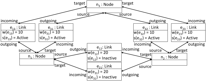
(a) Abstract syntax

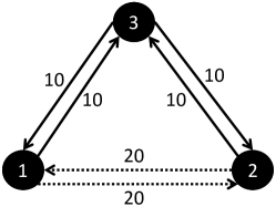
(b) Concrete syntax (directed)

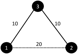
(c) Concrete syntax (undirected)

(d) *

[.3]

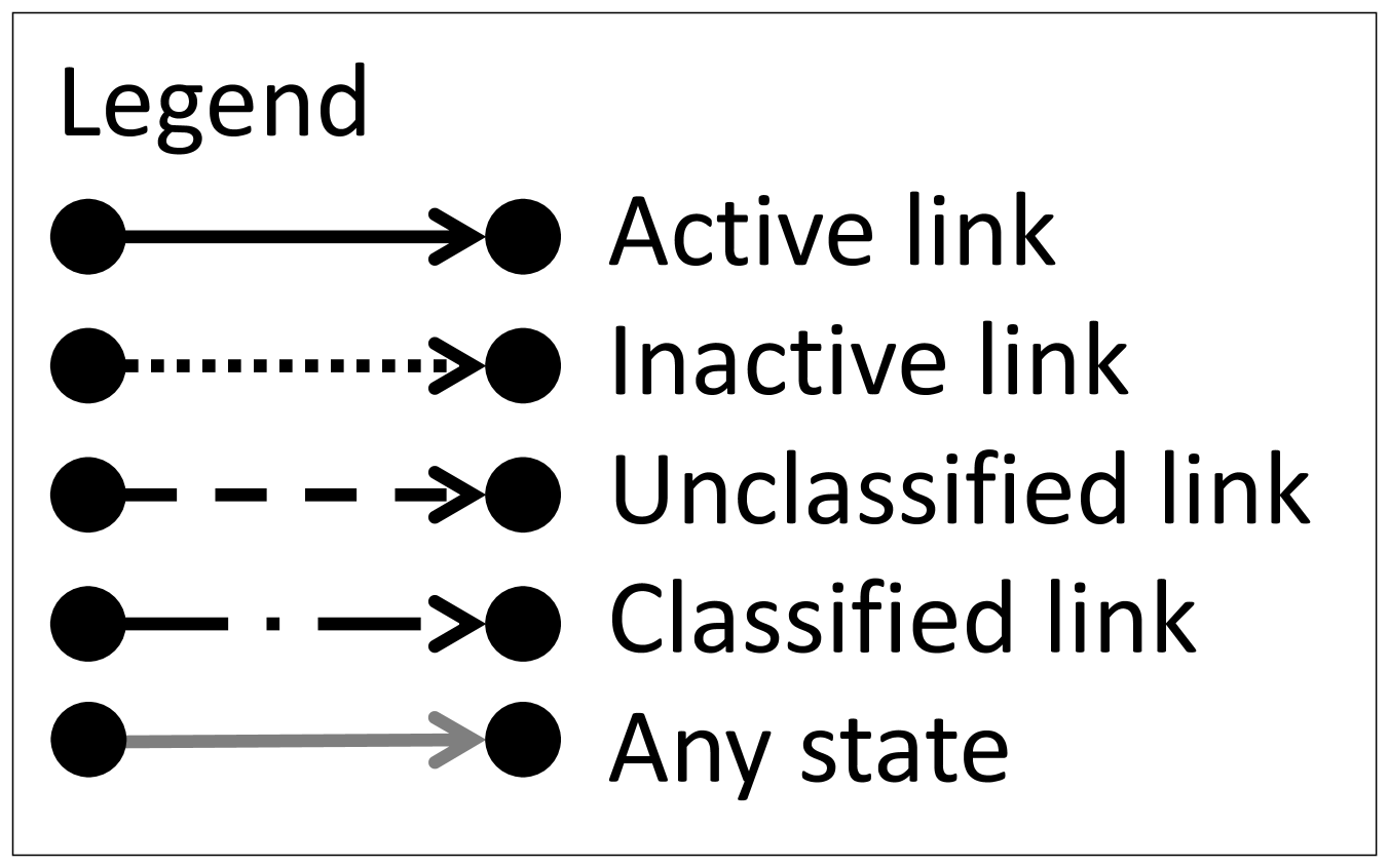
Figure 3: Triangle topology in abstract (top) and concrete (bottom) syntax

Controllability and restrictability

The TC developer may restrict the applicability of TC operations arbitrarily by introducing additional application restrictions. In contrast, context events may not be restricted because they represent the influence of the environment on the system. Instead, the TC developer has to ensure that applications of context event rules are handled appropriately. For similar reasons, it makes sense not to restrict the unclassification of links because it should always be possible to “revert” the classification of a link, e.g., if it turns out to be suboptimal. Therefore, we say that context events and link unclassification are unrestrictable.

2.4 Running Example: The Topology Control Algorithm kTC

As the running example of the following explanations, we chose the TC algorithm kTC. kTC [6] is a TC algorithm that, in batch mode, inactivates a link if this link is the unique weight-maximal link in some triangle and if the weight of this link is additionally at least $k$-times greater than the weight of the weight-minimal link in the same triangle. All links that do not fulfill this constraint are activated by kTC.

kTC it is a typical representative of a larger class of local TC algorithms, which operate based on local knowledge only [50, 51, 52]. This means that a node only knows about its immediate neighborhood, which is often characterized in terms of the maximum number of hops, i.e., the path length, between the node and its known neighbors. In the WSN community, local knowledge is often restricted to at most 2 hops because acquiring a larger local knowledge is typically infeasible due to, e.g., memory limitations of the sensor nodes and the message overhead to collect topology information [53]. Examples of other WSN algorithms that operate with 2-hop local knowledge are XTC [54], RNG [55], Yao Graph [56], and GG [57].

(a) Initial topology

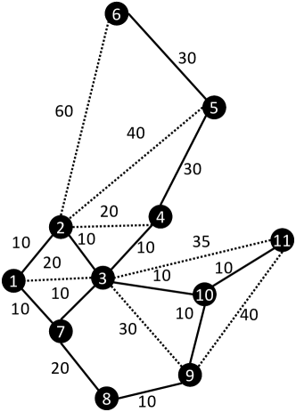
(b) Topology after executing kTC ($k{=}2$)

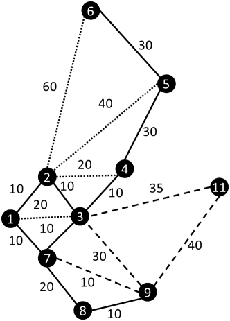
(c) Topology after adding links $e_{79}$ and $e_{97}$ and removing node $n_{\text{10}}$

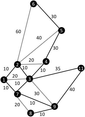
(d) Topology after re-executing kTC ($k{=}2$)

Figure 4: Incremental execution of kTC on a sample topology (link directions omitted)

Figure 4 illustrates the operation of kTC on a sample topology consisting of 11 nodes and 38 (directed) links, which are shown as 19 undirected links for presentation purposes. While $k$ should be in the interval $[1,\sqrt{2}]$ in realistic settings (see [6] for details), we chose $k{=}2$ for presentation purposes. Throughout this paper, we assume that context events do not interfere with the execution of TC, which is realistic because TC is typically carried out on a snapshot of the local neighborhood. In the initial topology of our example, all links are unclassified (Figure 4(a)). After executing kTC, 14 links are inactive and 24 links are active (Figure 4(b)). For instance, link $e_{25}$ is inactivated because its weight is at least $k$-times greater than the weight of link $e_{24}$, which is the weight of the shortest link in the triangle consisting of the links $e_{25}$, $e_{24}$, and $e_{45}$. Afterwards, the links $e_{79}$ and $e_{97}$ are added to the topology, e.g., because an obstacle between $n_{\text{7}}$ and $n_{\text{9}}$ disappeared, and node 10 is removed, e.g., because it was switched off. These context events lead to the unclassification of the directly neighbored links $e_{39}$, $e_{3\,11}$, $e_{79}$, and $e_{9\,11}$ (Figure 4(c)). In the last step, kTC repairs the topology incrementally by activating the links $e_{3\,11}$, $e_{9\,11}$, $e_{79}$ and by inactivating the links $e_{78}$ and $e_{39}$ (Figure 4(d)).

3 Specifying Consistent Topologies Using Graph Constraints

In this section, we characterize consistent and optimal output topologies of a TC algorithm by graph constraints. We begin with an introduction to the general concepts of graph patterns and graph constraints. Afterwards, we describe the concrete graph constraints that specify general structural consistency properties of topologies, general requirements of output topologies of TC algorithms in general, and the optimization goals of kTC in particular.

3.1 Graph Patterns and Graph Constraints

A graph pattern $p$ is a graph consisting of node variables and link variables, which are placeholders for nodes and links of a topology, plus a set of attribute constraints. An attribute constraint relates an attribute value of a node or link variable with attributes of the same or other node or link variables, e.g., using standard comparison operators such as = (equality), != (inequality).

A match $m$ of a graph pattern $p$ in a topology $G$ maps node (link) variables of $p$ to nodes (links) in $G$ such that (i) all attribute constraints are fulfilled, and (ii) node variables that are incident to a link variable are mapped to the source and target nodes of the link that the link variable is mapped to. Additionally, a match has to be injective, i.e., no two node (link) variables may be mapped to the same node (link). A pattern is satisfiable (unsatisfiable) if, among all possible topologies, at least one topology (no topology) contains a match of this pattern.

A graph constraint [42] consists of a premise pattern and a conclusion, which is a (potentially empty) set of conclusion patterns. The premise of a positive graph constraint is isomorphic to a subgraph of each conclusion pattern; the attribute constraints of the conclusion imply the attribute constraints of the premise. A negative graph constraint has no conclusion (denoted by $\emptyset$). A topology fulfills a graph constraint if any match of the premise of the constraint can be extended to a match of one of its conclusion patterns. This definition implies that a topology fulfills a negative graph constraint if (and only if) the topology does not contain any match of the premise. A topology violates a constraint if it does not fulfill the constraint.

3.2 Examples of Patterns and Graph Constraints

In the following, we use graph constraints to characterize structurally consistent topologies in general and valid output topologies of kTC in particular.

Structural constraints

We model topologies as simple, directed graphs, i.e., a topology may neither contain parallel links nor loops. Two edges are parallel if their source nodes and their target nodes are identical, respectively. A loop is a link whose source and target node are identical. The negative no-parallel-links constraint $C_{\text{no-par-links}}$ (shown in Figure 5(a)) and the negative no-loops constraint $C_{\text{no-loops}}$ (shown in Figure 5(b)) describe these structural consistency properties. The premise $p_{\text{no-par-links}}$ of the no-parallel-links constraint $C_{\text{no-par-links}}$ matches two distinct links $e_{ab,1}$ and $e_{ab,2}$ that both connect the same source node $n_{\text{a}}$ to the same target node $n_{\text{b}}$. The premise $p_{\text{no-loops}}$ of the no-loops constraint $C_{\text{no-loops}}$ matches a single link $e_{aa}$ that connects a node $n_{\text{a}}$ to itself.

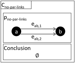
(a) $C_{\text{no-par-links}}$

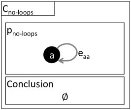
(b) $C_{\text{no-loops}}$

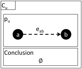
(c) $C_{\textrm{u}}$

Figure 5: Structural constraints $C_{\text{no-par-links}}$ and $C_{\text{no-loops}}$ and unclassified-link constraint $C_{\textrm{u}}$

From now on, we may assume that all topologies fulfill the no-parallel-links constraint $C_{\text{no-par-links}}$ and the no-loops constraint $C_{\text{no-loops}}$. This implies that neither $p_{\text{no-par-links}}$ nor $p_{\text{no-loops}}$ are unsatisfiable.

Unclassified-link constraint

After executing a TC algorithm, each link must be either active or inactive, i.e., the output topology does not contain unclassified links. This requirement avoids situations where a TC algorithm may immediately return without classifying all links. The negative unclassified-link constraint $C_{\textrm{u}}$ (shown in Figure 5(c)) describes this optimization goal. Its premise $p_{\text{u}}$ matches each unclassified link $e_{\text{ab}}$.

Algorithm-specific constraints

The aforementioned graph constraints are generic in the sense that either each topology fulfills them (structural constraints) or that each TC algorithm must ensure that its output topology fulfills them (unclassified-link constraint). Additionally, each TC algorithm has algorithm-specific graph constraints. In the following, we derive the algorithm-specific graph constraints of kTC.

The specification of kTC in [6] states that a link is inactive in the output topology of kTC if and only if it is the unique weight-maximal link in a triangle and if its weight is at least $k$-times greater than the weight of the weight-minimal link in the triangle; more formally:

$$\begin{split}\operatorname{s}(e_{\text{ab}})=\texttt{Inactive}&\;\Leftrightarrow\;e_{\text{ab}}\text{ is in a triangle with classified links }e_{\text{ac}},e_{\text{cb}}\\ &\wedge\;\operatorname{w}(e_{\text{ab}})>\max\left(\operatorname{w}(e_{\text{ac}}),\operatorname{w}(e_{\text{cb}})\right)\\ &\wedge\;\operatorname{w}(e_{\text{ab}})\geq k\cdot\min\left(\operatorname{w}(e_{\text{ac}}),\operatorname{w}(e_{\text{cb}})\right).\end{split}$$ (1)

The output topology consists of active and inactive links only because it fulfills the unclassified-link constraint $C_{\textrm{u}}$. Therefore, Equation 1 can be reformulated as follows: A link is active in the output topology if and only if it is not part of such a triangle where it is the unique weight-maximal link in a triangle and if its weight is at least $k$-times greater than the weight of the weight-minimal link in the triangle; more formally:

$$\begin{split}\operatorname{s}(e_{\text{ab}})=\texttt{Active}&\;\Leftrightarrow\;e_{\text{ab}}\text{ is in \emph{no} triangle with classified links }e_{\text{ac}},e_{\text{cb}}\\ &\text{ with }\operatorname{w}(e_{\text{ab}})>\max\left(\operatorname{w}(e_{\text{ac}}),\operatorname{w}(e_{\text{cb}})\right)\text{ and }\\ &\text{ with }\operatorname{w}(e_{\text{ab}})\geq k\cdot\min\left(\operatorname{w}(e_{\text{ac}}),\operatorname{w}(e_{\text{cb}})\right).\end{split}$$ (2)

The left-to-right implications of Equation 1 and Equation 2 correspond to the two kTC-specific constraints, shown in Figure 6 and described in the following.

The premise of the positive inactive-link constraint $C_{\textrm{i}}$ matches an inactive link $e_{\text{ab}}$, and its single conclusion pattern $c_{\textrm{i}}$ matches an inactive link $e_{\text{ab}}$ if it is part of a triangle (together with the classified links $e_{\text{ac}}$ and $e_{\text{cb}}$) where (i) $e_{\text{ab}}$has a weight greater than $\max(\operatorname{w}(e_{\text{ac}}),\operatorname{w}(e_{\text{cb}}))$, and (ii) $e_{\text{ab}}$has a weight greater than or equal to $k\cdot\min(\operatorname{w}(e_{\text{ac}}),\operatorname{w}(e_{\text{cb}}))$.

The premise of the negative active-link constraint $C_{\textrm{a}}$ matches any triangle consisting of an active link $e_{\text{ab}}$, and classified links $e_{\text{ac}}$ and $e_{\text{cb}}$ where (i) $e_{\text{ab}}$has a weight greater than $\max(\operatorname{w}(e_{\text{ac}}),\linebreak\operatorname{w}(e_{\text{cb}}))$, and (ii) $e_{\text{ab}}$has a weight greater than or equal to $k\cdot\min(\operatorname{w}(e_{\text{ac}}),\operatorname{w}(e_{\text{cb}}))$. The active-link constraint $C_{\textrm{a}}$ is a negative constraint because its conclusion is empty; it is only fulfilled for topologies that contain no such triangles.

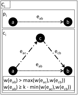
(a) $C_{\textrm{i}}$

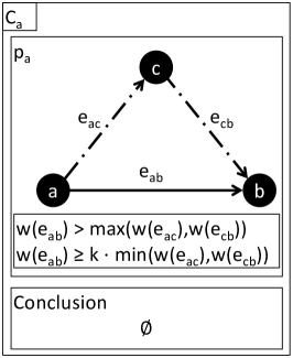
(b) $C_{\textrm{a}}$

Figure 6: Positive inactive-link constraint $C_{\textrm{i}}$ and negative active-link constraint $C_{\textrm{a}}$

To sum up, we have specified five graph constraints. The no-parallel-links constraint $C_{\text{no-par-links}}$ and the no-loops constraint $C_{\text{no-loops}}$ specify basic structural properties of topologies. The unclassified-link constraint $C_{\textrm{u}}$ specifies the general requirement that the output topology of a TC algorithm should consist only of classified links, Finally, the kTC-specific inactive-link constraint $C_{\textrm{i}}$ and active-link constraint $C_{\textrm{a}}$ jointly specify the optimization goal of the output topologies of the TC algorithm kTC.

3.3 Connectivity

Connectivity is a crucial consistency constraint of TC algorithms. Still, connectivity cannot be described in the framework of graph constraints as defined in [42] because it is a non-local constraint, i.e., connectivity cannot be expressed by a finite graph constraint consisting of premise and conclusion. A number of theoretical frameworks for expressing non-local graph constraints exists (e.g., [58]), but the constructive approach will still need to be extended to these frameworks. In this paper, we define different levels of topology connectivity, and we prove that the TC algorithm establishes the strongest type of connectivity for weakly consistent input topologies.

Definition 1 (Connectivity)

A path is an ordered sequence of links, where the target node of one link in the path is the source node of the next link. Based on this definition, we define the following three types of connectivity.

A topology fulfills physical connectivity $\hat{C}_{\text{p-conn}}$ if a directed path exists between any two nodes. The ‘hat’ notation make connectivity constraints easily distinguishable from other graph constraints.

A topology fulfills weak connectivity $\hat{C}_{\text{w-conn}}$ if a directed path consisting of active and unclassified links only exists between any two nodes.

A topology fulfills strongly connectivity $\hat{C}_{\text{s-conn}}$ if a directed path consisting of active links only exists between any two nodes.

The subsequent results immediately follow from the preceding definitions:

Corollary 2

Each strongly connected topology is also weakly connected, and each weakly connected topology is also physically connected.

Corollary 3

A weakly connected topology that also fulfills the unclassified-link constraint $C_{\textrm{u}}$ is strongly connected.

Physical connectivity is a structural constraint: If the underlying topology is not physically connected, a TC algorithm has cannot produce a connected output topology. Weak and strong connectivity are general constraints of TC algorithms: If the topology is at least weakly connected, messages can still be exchanged between all nodes by treating all unclassified links as if they were active. From Corollary 3 follows that, after the execution of a TC algorithm that enforces the unclassified-link constraint $C_{\textrm{u}}$, the output topology is strongly connected.

3.4 Consistency of Topologies

A topology is consistent w.r.t. a set of graph constraints if it fulfills all of these graph constraints. In our scenario, we distinguish three types of consistency: A topology is structurally consistent if it fulfills the topology constraints $C_{\text{no-loops}}$ and $C_{\text{no-par-links}}$. We require that any topology is structurally consistent. A topology is weakly consistent if it is structurally consistent and additionally fulfills the algorithm-specific graph constraints. A topology is strongly consistent if it is weakly consistent and additionally fulfills the unclassified-link constraint $C_{\textrm{u}}$, which means that each link is known either to be active or inactive. Strong consistency implies weak consistency, which in turn implies structural consistency.

In case of kTC, a topology is weakly consistent if it fulfills the topology constraints and the kTC-specific constraints $C_{\textrm{a}}$ and $C_{\textrm{i}}$, and it is strongly consistent if it additionally fulfills the unclassified-link constraint $C_{\textrm{u}}$. Table 1 gives an overview of the three different notions of consistency w.r.t. the kTC case study. A check mark (✓) indicates that the fulfillment of a particular type of consistency implies the fulfillment of a particular constraint.

Table 1: Overview of graph constraints constituting structural, weak, and strong consistency for the kTC example

Consistency	Structural Constraints			TC Constraints			kTC Constr.
	$C_{\text{no-par-links}}$	$C_{\text{no-loops}}$	$\hat{C}_{\text{p-conn}}$	$C_{\textrm{u}}$	$\hat{C}_{\text{w-conn}}$	$\hat{C}_{\text{s-conn}}$	$C_{\textrm{a}}$	$C_{\textrm{i}}$
Structural	✓	✓	✓
Weak	✓	✓	✓		✓		✓	✓
Strong	✓	✓	✓	✓	✓	✓	✓	✓

The following theorem states a useful observation: If we assume that the initial topology is physically connected and consists exclusively of unclassified links, then this topology is weakly consistent. If we manage to treat context events appropriately, we may keep the topology at least weakly consistent.

Theorem 4

A physically connected topology consisting entirely of unclassified links is weakly consistent.

Sketch of proof. Assume to the contrary that the topology violates at least one of the constraints of weak consistency. The structural constraints are guaranteed to hold. Additionally, the topology is also weakly connected because its unclassified-link subtopology equals the physical topology, which is connected. If the topology were to violate the negative active-link constraint $C_{\textrm{a}}$, the topology would contain a match of the premise of this constraint, which implies that there would be three classified links. If the topology were to violate the positive inactive-link constraint $C_{\textrm{i}}$, the topology would have to contain a match of the premise of these constraints, which implies the presence of at least one inactive link.

While structural consistency is guaranteed to hold for any topology, e.g., because a node will never use a link to communicate with itself, weak consistency may be violated by context events, which needs to be taken into account by the TC developer. Finally, invoking a TC algorithm for a weakly consistent topology should always produce a strongly consistent topology.

3.5 Proving Preservation of Connectivity for kTC

In the original paper that proposed kTC, the authors proved that kTC topologies are connected by showing that topologies produced by kTC contain, e.g., a minimum spanning tree [6]. In this paper, we directly prove that the output topology of kTC is strongly connected if the input topology is physically connected. We carry out the proof based on the kTC-specific graph constraints $C_{\textrm{a}}$ and $C_{\textrm{i}}$, only.

Theorem 5 (Strong consistency and strong connectivity)

A strongly consistent and physically connected topology is strongly connected.

Proof. Due to the assumption of physical connectivity, we know that a path of links (of arbitrary state) exists between any two nodes. Therefore, it suffices to show the following claim: The source and target node of each link are connected by a path of active links in the output topology. This trivially holds for the end nodes of active links. As the topology is strongly consistent, the active-link constraint $C_{\textrm{a}}$, the inactive-link constraint $C_{\textrm{i}}$, and the unclassified-link constraint $C_{\textrm{u}}$ are fulfilled, which implies that the topology only contains active and inactive links and that each inactive link $e$ is part of a triangle of active or inactive links having a weight that is smaller than the weight of $e$.

By induction, we show that the claim also holds for all inactive links $e_{\textrm{i},z},1\leq z\leq N_{\textrm{i}}$ with $N_{\textrm{i}}=|\{e\in E\mid\operatorname{s}(e)=\texttt{Inactive}\}|$: We consider the $N_{\textrm{i}}$ inactive links $e_{\textrm{i},1},\dots,e_{\textrm{i},N_{\textrm{i}}}$ of the topology ordered by weight, i.e., $\operatorname{w}(e_{\textrm{i},x})<\operatorname{w}(e_{\textrm{i},y})\Rightarrow x<y$.

Induction start ($z=1$): The weight-minimal inactive link, $e_{\textrm{i},1}$, is part of a triangle with two links, $e_{2}$ and $e_{3}$, which have a smaller weight and which are active because there is no inactive link with a less weight than $e_{\textrm{i},1}$ (Figure 7(a)). Therefore, the path $[e_{2},e_{3}]$ connects the start node of $e_{\textrm{i},1}$ with its target node, and the claim holds for link $e_{\textrm{i},1}$.

Induction step ($z\to z+1$): We now consider an inactive link $e_{\textrm{i},z+1}$ with $1\leq z\leq N_{\textrm{i}}{-}1$, which is part of a triangle with the two links $e_{2}$ and $e_{3}$ because the inactive-link constraint $C_{\textrm{i}}$ holds (Figure 7(b)). Without loss of generality, we assume that $e_{2}$ and $e_{3}$ are inactive. There exist integers $s$ and $t$ smaller than $z{+}1$ such that $e_{2}=e_{\textrm{i},s}$ and $e_{3}=e_{\textrm{i},t}$. As the claim has been proved for all inactive links of less weight than $e_{\textrm{i},z+1}$, a path $p_{2}$ of active links connects the source node with the target node of $e_{2}$, and a path $p_{3}$ of active links connects the source node with the target node of $e_{3}$. The joined paths $p_{2}$ and $p_{3}$ connect the source node of $e_{\textrm{i},z+1}$ to its target node, and the claim holds for link $e_{\textrm{i},z+1}$

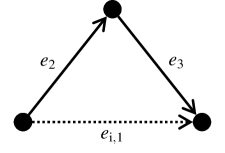
(a) Induction start ($z=1$)

(b) Induction step ($z\to z+1$ )

Figure 7: Sketches for the proof of Theorem 5

Theorem 6 (Weak consistency and weak connectivity)

A weakly consistent, physically connected topology is weakly connected.

Sketch of proof. The proof is analogous to the proof of Theorem 5. In this case, the constructed paths may contain active and unclassified links.

Corollary 7

The output topology of kTC is strongly connected if its input topology is physically connected.

Sketch of proof. The output topology of kTC is strongly consistent. Strong connectivity follows from Theorem 5 and from the assumption that the input topology of the TC algorithm is physically connected.

4 Specifying Topology Control and Context Event Rules Using Graph Transformation

In this section, we first present the basic concepts of graph transformation (GT) rules and programmed GT operations. Afterwards, we illustrate these concepts by specifying concrete TC and context event operations as GT rules and by specifying complete TC algorithms using programmed GT operations.

4.1 Graph Transformation

The following definitions are in concordance with standard literature in the GT community [22]. A GT rule consists of a left-hand side (LHS) pattern, a right-hand side (RHS) pattern and a number of application conditions. An application condition (AC) is a graph constraint whose premise contains the LHS. If the application condition is a positive constraint, it is called a positive application condition (PAC); otherwise it is called a negative application condition (NAC). The attribute constraints of the RHS pattern only consist of equality constraints. A GT rule has zero or more rule parameters, which may be node and link variables of the LHS or any variable that appears on the right side of an attribute constraint of the LHS or the RHS.

An application condition $\text{AC}_{x}$ is fulfilled for a match $m$ of the LHS of a GT rule if any possible extension of $m$ to a match of the premise of $\text{AC}_{x}$ may be extended to a match of at least one conclusion pattern of $\text{AC}_{i}$. This implies that a negative application condition is fulfilled for a match $m$ if the match cannot be extended to a match of the premise of the application condition.

A GT rule is applicable on a topology $G$ if a match $m$ of the LHS in $G$ exists that fulfills all application conditions of the rule. An application of a GT rule at a match $m$ in a topology $G$ is performed as follows: (i) All nodes (links) of $G$ that have a corresponding node (link) variable in the LHS but not in the RHS are removed. (ii) For each node (link) variable in the RHS that is not in the LHS, a new node (link) is added to $G$. (iii) Finally, the attribute constraints of the RHS are applied: In each attribute constraint, the expression to the right of the assignment operator is evaluated and the result is assigned to the variable to the left of the assignment operator. The co-match $m^{\prime}$ of the resulting graph $G^{\prime}$ maps each node (link) variable of RHS to a node (link) in $G^{\prime}$. After the successful application of a GT rule, the node and link variables of the RHS are bound, i.e., the resulting co-match maps each node (link) variable in the RHS to a fixed node (link) in $G$. In our context, rule parameters are also bound, which means that it has a fixed value that may not be re-assigned during a rule application. This permits us to pass the bound node (link) variables of a successful rule application as parameters to a second rule application.

In this paper, we use Story Diagrams [59], a programmed GT language [21], to structure GT rules into a control flow. A (programmed) GT operation is a directed graph that consists of activity nodes and activity edges. Additionally, it has a signature consisting of an operation name and a set of operation parameters. An activity node may either be a start node, stop node, story node, statement node, or foreach node. An activity edge interconnects two activity nodes and it may be labeled either with [Success] or [Failure]. If an activity edge is unlabeled, [Success] is assumed.

• A start node (depicted as solid circle) specifies the entry point of the control flow. Each operation has exactly one start node, which has no incoming activity edges and one unlabeled outgoing activity edge.

• A stop node (depicted as circle with a solid center) specifies an exit point of the control flow. Each operation has one or more stop nodes, and each stop node has at least one incoming activity edge and no outgoing activity edges.

• A story node (depicted as rounded rectangle) contains a single GT rule. It has at least one incoming activity edge and either one unlabeled outgoing activity edge or two outgoing activity edges labeled with [Success] and [Failure].

• A foreach node (denoted as a stacked rounded rectangle) is a special type of story node and contains a single GT rule.

• A statement node (depicted as rounded rectangle) contains an invocation of a GT operation. It has at least one incoming activity edge and one unlabeled outgoing activity edge.

When invoking a programmed GT operation, the execution begins at the start node and continues along the activity edges. What happens if the execution arrives at a particular story node, depends on the type of activity node:

• By definition, the execution may never return to the start node of a GT operation.

• When the execution arrives at a stop node, the operation returns.

• When the execution arrives at a story node, its GT rule is applied (if possible), and if the rule application was successful (unsuccessful), the execution continues along the [Success] ([Failure]) activity edge. If the rule application was successful, the link and node variables of the RHS of the rule are bound and may be re-used during subsequent rule applications or operation invocations.

• When the execution arrives at a foreach node, the following happens: (i) Allmatches of the LHS of the contained GT rule are determined; (ii) The contained GT rule is applied to each match, and for each successful rule application, the control flow continues along the activity edge labeled with [Success]; (iii) If all matches have been processed, the execution continues along the activity edge labeled with [Failure] and the set of collected matches is cleared.

• When the execution arrives at a statement node, the contained GT operation is invoked.

4.2 Examples of GT Rules and GT Operations

In the following, we present (i) the GT rules that describe basic building blocks of a TC algorihm, (ii) the GT operation that describes a basic TC algorithm, and (iii) the GT rules that describe context events

4.2.1 TC Rules

TC rules make up the basic building blocks of eacg TC algorithm. More specifically, according to our notion of TC algorithms, the marking step of any TC algorithm can be implemented as one or more GT operations that consist of the three TC operations link activation, link inactivation, and link unclassification. The latter is required, e.g., to revert unfavorable decisions or to propagate the unclassified flag to links that are affected by a context event in a non-local way. The corresponding GT rules $R_{\textrm{a}}$, $R_{\textrm{i}}$, and $R_{\textrm{u}}$ are shown in Figure 8, along with the two auxiliary rules $R_{\textrm{find-u}}$ and $R_{\textrm{find-ai}}$.

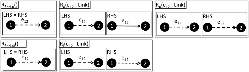
Figure 8: Topology control rules

• The unclassified-link identification rule $R_{\textrm{find-u}}$ identifies some unclassified link $e_{\text{12}}$ in the topology. As in this case, we use a compact notation (LHS=RHS) that only depicts one pattern if LHS and the RHS are identical.

• The classified-link identification rule $R_{\textrm{find-ai}}$ identifies some classified link $e_{\text{12}}$ in the topology, i.e., a link that is either active or inactive. This rule solely serves for illustrating a shorthand notation, applied in the following: In a strict sense, the RHS pattern of $R_{\textrm{find-ai}}$ is invalid because it contains the attribute constraint $e_{\text{12}}\in\{\texttt{Active},\texttt{Inactive}\}$. In the following, we follow the convention that this attribute constraint only applies to the LHS of the GT rule.

• The activation rule $R_{\textrm{a}}$ activates a given unclassified link $e_{\text{12}}$.

• The inactivation rule $R_{\textrm{i}}$ inactivates a given unclassified link $e_{\text{12}}$.

• The unclassification rule $R_{\textrm{u}}$ unclassifies a given classified (i.e., active or inactive) link $e_{\text{12}}$.

4.2.2 GT Operation basic-tc: A Basic TC Algorithm

Figure 9 shows the GT operation basic-tc, which serves as starting point for implementing the full specification of kTC in the following. basic-tc processes all unclassified links in a topology. For each unclassified link $e_{\text{12}}$, the activation rule $R_{\textrm{a}}$ is applied first if possible. If the application of $R_{\textrm{a}}$ was successful, the next unclassified link is processed, otherwise the inactivation rule $R_{\textrm{i}}$ is applied, if possible, and the execution returns to the story node containing the unclassified-link identification rule $R_{\textrm{find-u}}$. We emphasize that for most of the following explanations, the order of applications of $R_{\textrm{a}}$ and $R_{\textrm{i}}$ is arbitrary.

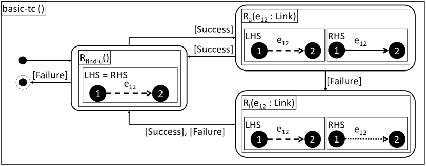
Figure 9: GT operation basic-tc, a basic TC algorithm that serves as template for further refinement

In this example, the activation rule $R_{\textrm{a}}$ is always applicable because $e_{\text{12}}$ is bound by $R_{\textrm{find-u}}$ and passed as parameter to $R_{\textrm{a}}$. Therefore, the inactivation rule $R_{\textrm{i}}$ is never tried in basic-tc. The basic TC algorithm basic-tc (i) enforces the unclassified-link constraint $C_{\textrm{u}}$ because the execution may only reach the stop node if there are no more unclassified links in the topology, (ii) preserves the inactive-link constraint $C_{\textrm{i}}$ because no link will ever be inactivated, but (iii) fails to preserve the active-link constraint $C_{\textrm{a}}$ because links are activated unconditionally.

4.2.3 Context Event Rules

Figure 10 shows the context event (CE) rules, which specify the possible modifications of the topology that are caused by the environment.

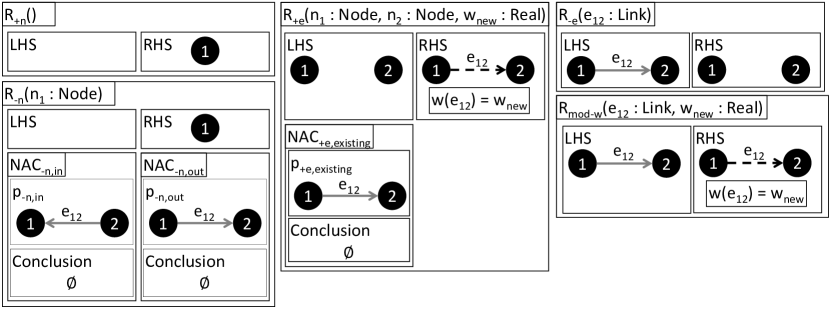
Figure 10: Context event rules

• The node addition rule $R_{\textrm{+n}}$ creates a new node $n_{\text{1}}$ and adds it to the topology by establishing a corresponding nodes-topology association between the node and the topology, which is not represented in the concrete syntax (as noted before). The empty LHS indicates that the rule is always applicable.

• The node removal rule $R_{\textrm{-n}}$ removes a single node $n_{\text{1}}$ from the topology by deleting (i) the corresponding nodes-topology association and (ii) the node $n_{\text{1}}$ itself. For conciseness, we write out $n_{\text{1}}$ only in the parameter list, but abbreviate it as encircled 1 inside the rule. The two negative application conditions, $\text{NAC}_{\text{-n},\text{in}}$ and $\text{NAC}_{\text{-n},\text{out}}$, prevent dangling links by ensuring that the node to be removed has neither incoming nor outgoing links.

• The link addition rule $R_{\textrm{+e}}$ creates an unclassified link with the given source node $n_{\text{1}}$ and target node $n_{\text{2}}$, assigns it the given weight $w_{\text{new}}$, and adds it to the topology by creating a corresponding links-topology association between the link and the topology. The negative application condition $\text{NAC}_{\text{+e,existing}}$ ensures that a rule application does not insert a parallel link from node $n_{\text{1}}$ to node $n_{\text{2}}$.

• The link removal rule $R_{\textrm{-e}}$ removes a given link $e_{\text{12}}$ from the topology by deleting (i) the corresponding links-topology association and (ii) the link itself.

• The weight modification rule $R_{\textrm{mod-w}}$ sets the weight of the given link $e_{\text{12}}$ to $w_{\text{new}}$ and unclassifies it.

4.3 Constraint and Consistency Preservation

In the following, we introduce the concept of constraint preservation to describe how applying a GT rule affects the consistency of a topology: An application of a GT rule $R_{x}$ preserves a graph constraint $C_{y}$ on a topology that fulfills $C_{y}$ if the topology still fulfills $C_{y}$ after applying $R_{x}$. A GT rule $R_{x}$ preserves a graph constraint $C_{y}$ if $R_{x}$ preserves $C_{y}$ on any topology. These definitions can be lifted to the concept of consistency in a natural way: A GT rule $R_{x}$ preserves weak (strong) consistency if it preserves all graph constraints that make up weak (strong) consistency. An application condition $\text{AC}_{z}$ of a GT rule $R_{x}$ is redundant w.r.t. a graph constraint $C_{y}$ if $\text{AC}_{z}$ is always fulfilled under the assumption that $C_{y}$ holds prior to each application of $R_{x}$. This means that we may remove $\text{AC}_{z}$ from $R_{x}$ without threatening consistency preservation.

Given a topology that fulfills a positive graph constraint, a rule application preserves the constraint on the topology (i) if each new match of its premise may be extended to a match of the conclusion, and (ii) if each old match of its premise that also exists after the rule application may still be extended to a match of its conclusion after the rule application. Accordingly, given a topology that fulfills a negative graph constraint, a rule application preserves the constraint on the topology if the rule application does not create a new match of the premise of the constraint.

Preservation of structural constraints

The structural constraints $C_{\text{no-par-links}}$ and $C_{\text{no-loops}}$ may only be violated by adding a link, i.e., by applying the link addition rule $R_{\textrm{+e}}$. This rule, however, has already been defined to preserve these constraints: (i) The negative application condition $\text{NAC}_{\text{+e,existing}}$ prevents any applications of $R_{\textrm{+e}}$ that would result in a parallel link between node $n_{\text{1}}$ and node $n_{\text{2}}$, and (ii) the required injectivity of matches of the LHS enforces that the node $n_{\text{1}}$ and node $n_{\text{2}}$ are distinct, thereby preventing the new link $e_{\text{12}}$ to have identical source and target nodes.

Examples of constraint violation

Figure 11 shows four examples that illustrate how applying one of the TC or context event rules leads to a constraint violation. These violations clearly call for a modification of the rules to avoid constraint violations. In all examples, $k$ equals $2$.

In Figure 11(a), the topology that results from applying the activation rule $R_{\textrm{a}}$ to link $e_{12}$ violates the active-link constraint $C_{\textrm{a}}$ because the weight of $e_{12}$ is more than $k$-times greater than the weight of the weight-minimal link $e_{13}$.

In Figure 11(b), the topology that results from applying the link removal rule $R_{\textrm{-e}}$ to link $e_{13}$ violates the inactive-link constraint $C_{\textrm{i}}$ because the match of the premise of the constraint can no longer be extended to a match of its conclusion.

In Figure 11(c), the topology that results from applying the inactivation rule $R_{\textrm{i}}$ to link $e_{13}$ violates the active-link constraint $C_{\textrm{a}}$. Even though the links formed a triangle prior to applying $R_{\textrm{i}}$, the inactive-link constraint $C_{\textrm{i}}$ was not violated because $e_{13}$ was unclassified.

In Figure 11(d), the topology that results from applying the weight modification rule $R_{\textrm{mod-w}}$ to link $e_{13}$ with $w_{\text{new}}=3$ violates the inactive-link constraint $C_{\textrm{i}}$ because the single match of the conclusion that extends the match of the premise is destroyed by the unclassification of link $e_{13}$, Remarkably, the inactive-link constraint $C_{\textrm{i}}$ would not have been violated if $e_{13}$ had remained active because the weight of $e_{13}$ has even decreased from 5 to 3.

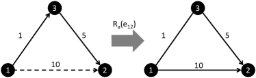
(a) Violation of $C_{\textrm{a}}$ caused by applying $R_{\textrm{a}}$

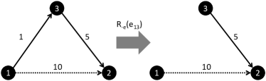
(b) Violation of $C_{\textrm{i}}$ caused by applying $R_{\textrm{-e}}$

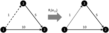
(c) Violation of $C_{\textrm{a}}$ caused by applying $R_{\textrm{i}}$

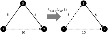
(d) Violation of $C_{\textrm{i}}$ caused by applying $R_{\textrm{mod-w}}$

Figure 11: Examples of constraint violations caused by rule applications ($k=2$)

5 Refining Topology Control and Context Events Rules to Preserve Graph Constraints

The examples at the end of Section 4.3 clearly indicate that basic-tc, the template GT operation for developing kTC, enforces the unclassified-link constraint $C_{\textrm{u}}$, but fails to preserve even weak consistency. In this section, the TC and context event rules and the GT operation basic-tc are refined to achieve the following goals.

1. The refined TC rules and context event rules preserve weak consistency.

2. Each refined unrestrictable rule is applicable whenever its corresponding original rule is applicable (see Section 2.3).

3. The refined GT operation basic-tc turns each weakly consistent input topology into a strongly consistent output topology.

After accomplishing these goals, basic-tc will be a valid GT-based specification of kTC. For this reason, we will refer to the refined GT operation basic-tc as ktc from now on. The structure of this section is depicted in Figure 12 and is shortly summarized in the following paragraphs.

Figure 12: Structure of Section 5

Goal G1 aims at deriving the so-called weakest precondition [60] for each GT rule and can be achieved by applying the constructive approach first presented in [42] and refined later for attributes in [43]. This approach takes a set of GT rules and graph constraints as input and refines each GT rule to ensure that all GT rules preserve all the graph constraints. In Section 5.1, we describe the refinement algorithm in detail and apply it to the TC and context event rules, finally achieving goal G1. However, only applying the constructive approach is not sufficient in our application scenario for the following reasons.

1. The additional application conditions, which have been introduced during the refinement of the TC and context event rules, restrict their applicability. While such restrictions are perfectly reasonable (and desirable) for TC rules, restricting context event rules is unrealistic because these rules represent (non-controllable!) modifications of the topology that are caused by the environment. For similar reasons, the applicability of the unclassification rule $R_{\textrm{u}}$ may not be restricted. In the following, we subsume the context event rules and the unclassification rule $R_{\textrm{u}}$ under the term unrestrictable (GT) rules.

   In Section 5.2, we propose to translate the application conditions of the unrestrictable rules that have been introduced during the rule refinement into appropriate handler (GT) operations. This step is one of the major contributions of this paper. In the course of this step, the additional application conditions of the unrestrictable GT rules are dropped under the assumption that the corresponding handler operation is always invoked immediately after the application of a context event rule; upon the completion of this step, goal G2 will be fulfilled.

2. The additional application conditions of the activation rule $R_{\textrm{a}}$ and the inactivation rule $R_{\textrm{i}}$ may (and will) lead to situations where the currently considered unclassified link $e_{\text{12}}$ can be processed by neither of these rules. For this reason, ktc may not terminate in certain situations.

   In Section 5.3, we propose to insert a handler operation that is invoked prior to applying the activation rule $R_{\textrm{a}}$ or the inactivation rule $R_{\textrm{i}}$. This operation systematically unclassifies links that would prevent the application of both the activation rule $R_{\textrm{a}}$ and the inactivation rule $R_{\textrm{i}}$. We prove that the modified GT operation ktc always terminates, thereby achieving goal G3.

5.1 Refining Graph Transformation Rules to Preserve Graph Constraints

In this section, we tackle goal G1, the preservation of weak consistency, and introduce the refinement algorithm that builds on the constructive approach presented in [42, 43]. We start by introducing basic concepts. Then, we describe the general algorithm and apply it to the TC and context event rules.

5.1.1 Basic Concepts: Post-conditions of GT Rules and Gluings of Patterns

In Section 4, we have introduced application conditions, which restrict the applicability of GT rules and which are checked before the corresponding rule modifies any match. Therefore, application conditions are also called pre-conditions. In the general case, a GT rule may also be equipped with a set of post-conditions, which have the same structure as pre-conditions, but are checked after the application of their rules. The premise of a post-condition extends the RHS of its rule in the same fashion as the premise of a pre-condition extends the LHS. Conclusions of pre- and post-conditions extend their premises as explained beforehand.

Any violation of a pre-condition or a post-condition of a rule blocks its execution; as a consequence, a GT engine has to roll back the application of a rule if this application results in a violation of one of its post-conditions. Fortunately, any post-condition of a rule can be translated into an equivalent pre-condition (and vice versa). It is even possible to translate arbitrary graph constraints into post- or pre-conditions of a given GT rule such that this rule preserves these graph constraints; this is the fundamental idea of the constructive approach in [42].

The approach relies on the construction of so-called gluings, which are combinations of the RHS (LHS) of a GT rule and the premises and conclusions of the regarded graph constraints. More precisely, a gluing $g_{\ell,r}$ of patterns $p_{\ell}$ and $p_{r}$ is a graph pattern that represents one possible overlap of $p_{\ell}$ and $p_{r}$. We denote variables of $p_{\ell}$ with numbers ($1$, $2$, etc.), variables of $p_{r}$ with lowercase letters ($a$, $b$, etc.), and variables of $g_{\ell,r}$ with uppercase letters plus their corresponding variables in $p_{\ell}$ and $p_{r}$ (e.g., $A[1,a]$). Injective mappings $m_{\ell}$ and $m_{r}$ exist that assign to each node (link) variable of $p_{\ell}$ and $p_{r}$ a corresponding node (link) variable in $g_{\ell,r}$. Each node (link) variable in $g_{\ell,r}$ has at least one corresponding node (link) variable in $p_{\ell}$ and $p_{r}$, and at least one node variable of $g_{\ell,r}$ must correspond to node variables in $p_{\ell}$ and $p_{r}$, i.e., the patterns $p_{\ell}$ and $p_{r}$ must indeed overlap. The attribute constraints of $g_{\ell,r}$ correspond to the joint attribute constraints of $p_{\ell}$ and $p_{r}$ with appropriately relabeled node (link) variables.

For example, Figure 14 (on page 14) and Table 3 show all six possible gluings $g_{\textrm{u},\textrm{i},z\,,\,1\leq z\leq 6}$ of the RHS of the unclassification rule $R_{\textrm{u}}$ and the premise of the inactive-link constraint $C_{\textrm{i}}$ using a graphical and a compact tabular representation, respectively. Each gluing has at most three node variables because each original pattern has two node variables and because at least one node variable of the two patterns must be glued together. Each column of Table 3 corresponds to one gluing $g_{\textrm{u},\textrm{i},k}$, and each row corresponds to one of the up to three node variables A, B, and C of the gluing. In this example, the node variable $1$ of the unclassification rule $R_{\textrm{u}}$ and the node variable a of the inactive-link constraint $C_{\textrm{i}}$ are mapped to the node variable A of gluing $g_{\textrm{u},\textrm{i},1}$. Note that the resulting set of attribute constraints of gluing $g_{\textrm{u},\textrm{i},1}$ is unsatisfiable: $\operatorname{s}(e_{AB})=\texttt{Active}$ (resulting from $R_{\textrm{u}}$) and $\operatorname{s}(e_{AB})=\texttt{Inactive}$ (resulting from $C_{\textrm{i}}$).

5.1.2 Description of Refinement Algorithm

In [42], Heckel and Wagner describe the constructive approach for enforcing constraint preservation of GT rules, which forms the centerpiece of the first step in our approach. On an abstract level, the refinement algorithm works by iteratively considering all pairs of rules and constraints: A rule $R_{x}$ and a graph constraint $C_{y}$ serve as input to the refinement procedure. The refinement procedure results in zero or more additional application conditions of $R_{x}$ These application conditions prevent any application of $R_{x}$ that may produce violations of $C_{y}$. In our scenario, we may assume that TC or context event rules are only applied to topologies that are weakly consistent. Figure 13 gives a detailed overview of the refinement procedure of a particular rule $R_{x}$ and a particular constraint $C_{y}$, which works as follows:

1. We construct all gluings $g_{x,y,z}$ of the RHS of rule $R_{x}$ and of the premise of constraint $C_{y}$.

2. Each gluing $g_{x,y,z}$ serves as the premise of a new post-condition $\text{PC}_{x,y,z}$. Then, the premise is extended to the basic conclusion pattern $c^{\prime}_{x,y,z,1}$ of the post-condition by extending the premise with all node and link variables and the attribute constraints that are part of the conclusion but not of the premise of the constraint $C_{y}$.

3. The set of reduced conclusion patterns $c^{\prime}_{x,y,z,r\,,\,r\geq 2}$ of the post-condition is the set of all patterns that results from merging one or more node variables of the basic conclusion $c^{\prime}_{x,y,z,1}$. We may only merge node variables that are not contained in the premise. The incident link variables of merged node variables are merged accordingly. The conclusion $c^{\prime}_{x,y,z}$ of post-condition $\text{PC}_{x,y,z}$ consists of the basic conclusion pattern and the set of reduced conclusion patterns $c{}_{x,y,z}$.

4. An application condition $\text{AC}_{x,y,z}$ is obtained from a post-condition $\text{PC}_{x,y,z}$ by applying rule $R_{x}$ in reverse order to the premise and to each conclusion pattern of $\text{PC}_{x,y,z}$. All node and link variables and all attribute constraints that appear in the RHS but not in the LHS of $R_{x}$ are removed from $\text{AC}_{x,y,z}$, and copies of all node and link variables and attribute constraints that appear in the LHS but not in the RHS of $R_{x}$ are added to $\text{AC}_{x,y,z}$.

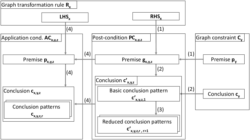
Figure 13: Overview of the four steps of the rule refinement procedure

To sum up, the refinement procedure first translates the graph constraint to post-conditions of the GT rule in steps (1)–(3), which are then translated to equivalent pre-conditions in step (4). We categorize gluings into three groups based on the satisfiability of their corresponding application condition:

• Unsatisfiable gluing: If it is impossible to find a match of a gluing in any topology, we say that this gluing is unsatisfiable. For instance, a gluing that contains contradictory link state constraints for a particular link variable is unsatisfiable. An unsatisfiable gluing $g_{x,y,z}$ corresponds to an application condition that is always fulfilled because no match of the LHS of the rule may ever be extended to a match of premise $p_{x,y,z}$. As explained in Section 5.1.1, $g_{\textrm{u},\textrm{i},1}$ is an example of an unsatisfiable gluing.

• Redundant application condition: An application condition of a GT rule is redundant if is fulfilled under the assumption that the structural graph constraints ($C_{\text{no-par-links}}$ and $C_{\text{no-loops}}$) are fulfilled prior to any application of the rule.

• Restrictive application condition: Any application condition that does not fall into one of the two above mentioned groups truly restricts the applicability of a rule, i.e., it is a (truly) restrictive application condition.

From these explanations, it is clear that we only need to add restrictive application conditions to the GT rules and discard application conditions that originate from an unsatisfiable gluing or are redundant.

The rule refinement procedure sketched above has the following properties, which are essential for the development of a TC algorithm that turns a weakly into a strongly consistent topology [42]: (i) The added application conditions are strong enough to prevent any application of GT rule $R_{x}$ that would transform a topology $G$ fulfilling $C_{y}$ into a topology $G^{\prime}$ that violates $C_{y}$, i.e., they are sufficient. (ii) The added application conditions are weak enough to allow any application of GT rule $R_{x}$ that does not transform a topology $G$ fulfilling $C_{y}$ into a topology $G^{\prime}$ that violates $C_{y}$, i.e., they are necessary.

Table 2 provides an overview of the subsequent sections that describe the application of the refinement algorithm to the GT rules.

Table 2: Overview of iterations of the refinement algorithm

Rules	$C_{\textrm{i}}$	$C_{\textrm{a}}$
TC ($R_{\textrm{u}}$, $R_{\textrm{a}}$, $R_{\textrm{i}}$)	Section 5.1.3	Section 5.1.4
Context events ($R_{\textrm{+n}}$, $R_{\textrm{-n}}$, $R_{\textrm{+e}}$, $R_{\textrm{-e}}$, $R_{\textrm{mod-w}}$)	Section 5.1.5	Section 5.1.6

5.1.3 Refining Topology Control Rules to Preserve the Inactive-Link Constraint

We begin with refining the TC rules, i.e., the unclassification rule $R_{\textrm{u}}$, the activation rule $R_{\textrm{a}}$, and the inactivation rule $R_{\textrm{i}}$, to preserve the positive inactive-link constraint $C_{\textrm{i}}$.

$R_{\textrm{u}}$ + $C_{\textrm{i}}$ The six resulting gluings $g_{\textrm{u},\textrm{i},z\,,\,1\leq z\leq 6}$ of the RHS of the unclassification rule $R_{\textrm{u}}$ and the premise of the inactive-link constraint $C_{\textrm{i}}$ (the result of step (1)) are shown in Figure 14 and Table 3 using a graphical and a compact tabular representation, respectively.

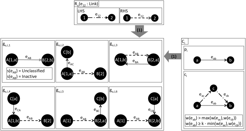
Figure 14: Gluings $g_{\textrm{u},\textrm{i},x}$ of the RHS of the unclassification rule $R_{\textrm{u}}$ and the premise of the inactive-link constraint $C_{\textrm{i}}$

Table 3: Overview of gluings of the RHS of the unclassification rule $R_{\textrm{u}}$ and the inactive-link constraint $C_{\textrm{i}}$

Variables in $R_{\textrm{u}}$ and Gluing $g_{\textrm{u},\textrm{i},x}$	Origin in $C_{\textrm{i}}$ (per Gluing)
	$g_{\textrm{u},\textrm{i},1}$	$g_{\textrm{u},\textrm{i},2}$	$g_{\textrm{u},\textrm{i},3}$	$g_{\textrm{u},\textrm{i},4}$	$g_{\textrm{u},\textrm{i},5}$	$g_{\textrm{u},\textrm{i},6}$
$A=m_{\ell}(1)$	a	a	b	b	-	-
$B=m_{\ell}(2)$	b	-	a	-	a	b
C	-	b	-	a	b	a

The gluings can be categorized into the aforementioned three categories as follows.

• Unsatisfiable gluing: Gluing $g_{\textrm{u},\textrm{i},1}$ is unsatisfiable due to the conflicting link state constraints that require $e_{\text{AB}}$ to be unclassified (from $R_{\textrm{u}}$) and inactive (from $C_{\textrm{i}}$) at the same time, and is discarded during step (2).

• Redundant PAC: Figure 15 illustrates that gluing $g_{\textrm{u},\textrm{i},3}$ corresponds to a redundant PAC: The affected link $e_{\text{AB}}$ is never part of the triangle of links that is a match of the conclusion of the inactive-link constraint $C_{\textrm{i}}$. Due to the assumption that the topology fulfills the inactive-link constraint $C_{\textrm{i}}$ before applying the unclassification rule $R_{\textrm{u}}$, the PAC is always fulfilled and may be safely ignored.

  

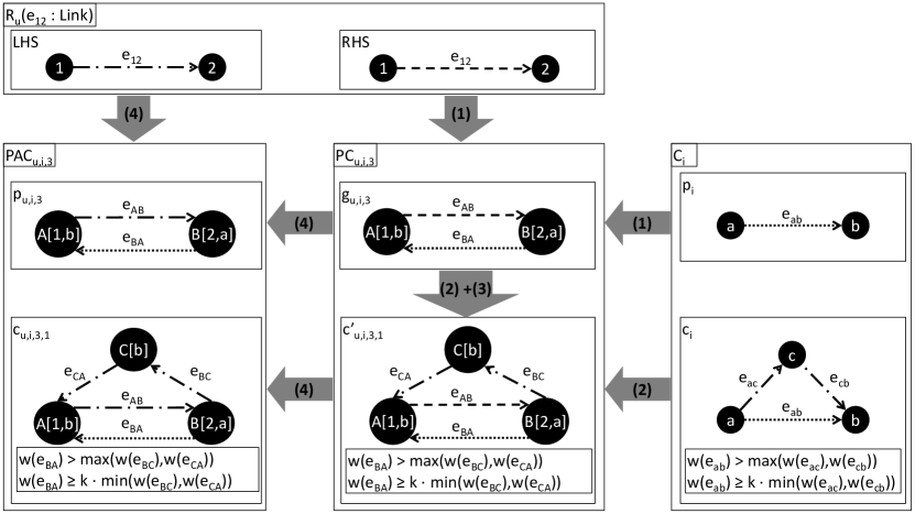
  Figure 15: Transformation of the gluing $g_{\textrm{u},\textrm{i},3}$ into the redundant application condition  $\text{PAC}_{\textrm{u},\textrm{i},3}$

• Restrictive PACs: The gluings $g_{\textrm{u},\textrm{i},2}$, $g_{\textrm{u},\textrm{i},4}$, $g_{\textrm{u},\textrm{i},5}$, and $g_{\textrm{u},\textrm{i},6}$ correspond to four additional non-redundant PACs of $R_{\textrm{u}}$. In the following, we describe the application of the refinement procedure to $g_{\textrm{u},\textrm{i},2}$ in detail.

Gluing $g_{\textrm{u},\textrm{i},2}$ is satisfiable; therefore, it serves as the premise of the new post-condition $\text{PC}_{\textrm{u},\textrm{i},2}$, as shown in Figure 16.

Figure 16: Transformation of gluing $g_{\textrm{u},\textrm{i},2}$ into the positive application condition $\text{PAC}_{\textrm{u},\textrm{i},2}$

In step (3), we obtain the basic conclusion $c{{}^{\prime}}_{\textrm{u},\textrm{i},2,1}$ by adding node variable $D$, which corresponds to node variable $c$ in $c_{\textrm{i}}$. In step (4), three reduced conclusion patterns $c{{}^{\prime}}_{\textrm{u},\textrm{i},2,r\,;\,2\leq r\leq 4}$ are obtained by merging node variable D with the node variables A, B, and C, respectively. All three reduced conclusions are not considered further on because they are unsatisfiable due to either loops (for $c{{}^{\prime}}_{\textrm{u},\textrm{i},2,2}$) or parallel link variables (for $c{{}^{\prime}}_{\textrm{u},\textrm{i},2,3}$ and $c{{}^{\prime}}_{\textrm{u},\textrm{i},2,4}$). Therefore, in step (4), only the basic conclusion $c{{}^{\prime}}_{\textrm{u},\textrm{i},2,1}$ is transformed into a conclusion pattern of the positive application condition $\text{PAC}_{\textrm{u},\textrm{i},2}$ of the unclassification rule $R_{\textrm{u}}$. Intuitively speaking, the new application condition requires that for each outgoing link of the source node of the affected link $e_{\text{12}}$, a triangle of links must exist that matches the conclusion of the inactive-link constraint $C_{\textrm{i}}$. This additional triangle ensures that even if unclassifying link $e_{\text{12}}$ may destroy a match of the conclusion of $C_{\textrm{i}}$, there is at least one more match of $c_{\textrm{i}}$, which ensures that $C_{\textrm{i}}$ is preserved. As a result of this refinement step, four new non-redundant application conditions $\text{PAC}_{\textrm{u},\textrm{i},2}$, $\text{PAC}_{\textrm{u},\textrm{i},4}$, $\text{PAC}_{\textrm{u},\textrm{i},5}$, and $\text{PAC}_{\textrm{u},\textrm{i},6}$ were added to the unclassification rule $R_{\textrm{u}}$ shown in Figure 17.

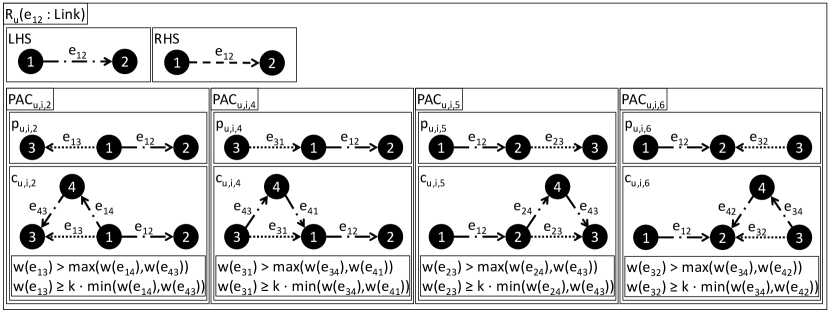
Figure 17: Refined unclassification rule $R_{\textrm{u}}$ with four additional application conditions $\text{PAC}_{\textrm{u},\textrm{i},z\,;\,z\in\{2,4,5,6\}}$

$R_{\textrm{a}}$ + $C_{\textrm{i}}$ The six possible gluings $g_{\textrm{a},\textrm{i},z\,,\,1\leq z\leq 6}$ of the RHS of the activation rule $R_{\textrm{a}}$ and the premise of the inactive-link constraint $C_{\textrm{i}}$ are almost identical to the gluings $g_{\textrm{u},\textrm{i},z\,,\,1\leq z\leq 6}$, shown in Figure 14. The major difference is that the link state constraint of $e_{\text{AB}}$ originating from the activation rule $R_{\textrm{a}}$ is now $\operatorname{s}(e_{\text{AB}})=\texttt{Active}$ in all gluings. In this case, the gluings and their corresponding application conditions can be categorized as follows:

• Unsatisfiable gluing: Gluing $g_{\textrm{a},\textrm{i},1}$ is unsatisfiable due to the conflicting attribute constraints $\operatorname{s}(e_{\text{AB}})=\texttt{Active}$ (from $R_{\textrm{a}}$) and $\operatorname{s}(e_{\text{AB}})=\texttt{Inactive}$ (from $C_{\textrm{i}}$), and is discarded during step (2).

• Redundant PACs: The remaining five gluings $g_{\textrm{a},\textrm{i},2}$ to $g_{\textrm{a},\textrm{i},6}$ correspond to redundant PACs as illustrated for $g_{\textrm{a},\textrm{i},2}$ in Figure 18.

  

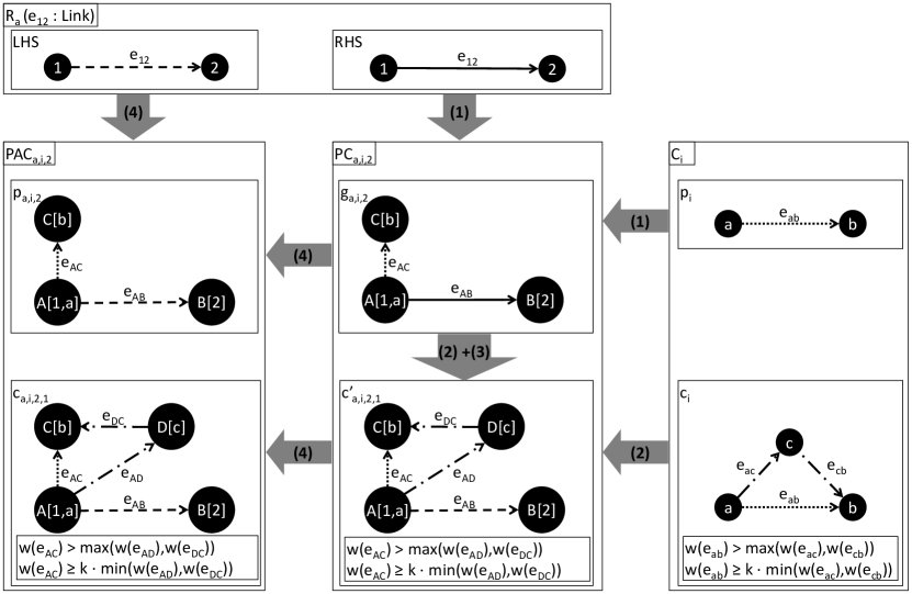
  Figure 18: Transformation of gluing $g_{\textrm{a},\textrm{i},2}$ into the redundant application condition $\text{PAC}_{\textrm{a},\textrm{i},2}$

  We show only the basic conclusion because, as discussed previously, the reduced conclusions are all unsatisfiable due to loops or parallel link variables. Note that, if any outgoing link of node variable A was inactive prior to applying the activation rule $R_{\textrm{a}}$, then it would be part of a triangle of links that matches the conclusion of $C_{\textrm{i}}$, and $e_{\text{AB}}$ is not part of this triangle because it is unclassified. Therefore, the resulting application condition $\text{PAC}_{\textrm{a},\textrm{i},2}$ is always fulfilled and can be safely ignored.

• Restrictive PACs: None of the gluings corresponds to a restrictive PAC. Therefore, as a result of this refinement step, no application conditions need to be added to the activation rule $R_{\textrm{a}}$.

$R_{\textrm{i}}$ + $C_{\textrm{i}}$ The six gluings $g_{\textrm{i},\textrm{i},z\,,\,1\leq z\leq 6}$ of the RHS of the inactivation rule $R_{\textrm{i}}$ and the premise of the inactive-link constraint $C_{\textrm{i}}$ are similar to the gluings $g_{\textrm{u},\textrm{i},z\,,\,1\leq z\leq 6}$, shown in Figure 14. The major difference is that the link state constraint of $e_{\text{AB}}$ is now $\operatorname{s}(e_{\text{AB}})=\texttt{Inactive}$ in all gluings. In this case, the gluings and their corresponding application conditions can be categorized as follows:

• Unsatisfiable gluing: None of the gluings $g_{\textrm{i},\textrm{i},z\,,\,1\leq z\leq 6}$ is unsatisfiable.

• Restrictive PAC: Figure 19 shows that the gluing $g_{\textrm{i},\textrm{i},1}$ corresponds to an additional PAC of the inactivation rule $R_{\textrm{i}}$.

  

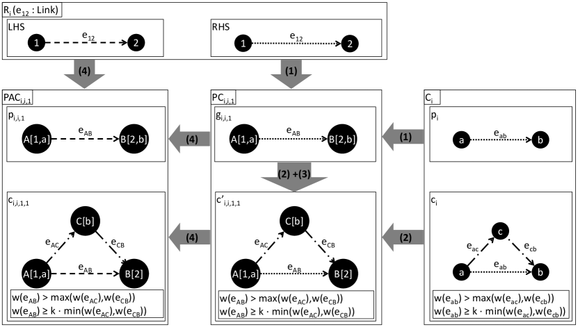
  Figure 19: Transformation of the gluing $g_{\textrm{i},\textrm{i},1}$ into the restrictive application condition $\text{PAC}_{\textrm{i},\textrm{i},1}$

  Gluing $g_{\textrm{i},\textrm{i},1}$ serves as the premise of the post-condition $\text{PC}_{\textrm{i},\textrm{i},1}$. We construct the conclusion to $\text{PC}_{\textrm{i},\textrm{i},1}$ by extending $g_{\textrm{i},\textrm{i},1}$ with a new node variable C, which corresponds to the node variable c in $C_{\textrm{i}}$. The new positive application condition $\text{PAC}_{\textrm{i},\textrm{i},1}$ is obtained by applying $R_{\textrm{i}}$ in reverse order.

• Redundant PACs: As in the case of the activation rule $R_{\textrm{a}}$, the remaining five gluings $g_{\textrm{i},\textrm{i},2}$ to $g_{\textrm{i},\textrm{i},6}$ result in redundant PACs due to the assumption that the topology fulfills the inactive-link constraint $C_{\textrm{i}}$ prior to any application of the inactivation rule $R_{\textrm{i}}$.

As a result of this refinement step, the non-redundant positive application condition $\text{PAC}_{\textrm{i},\textrm{i},1}$ was added to the inactivation rule $R_{\textrm{i}}$.

5.1.4 Refining Topology Control Rules to Preserve the Active-Link Constraint

Next, we refine the TC rules, i.e., the activation rule $R_{\textrm{a}}$, the inactivation rule $R_{\textrm{i}}$, and the unclassification rule $R_{\textrm{u}}$, to preserve the negative active-link constraint $C_{\textrm{a}}$. The active-link constraint $C_{\textrm{a}}$ is a negative constraint, which is transformed into additional negative application conditions of the affected TC rules. In this iteration, step (2) and step (3) of the refinement procedure are skipped because the conclusion of the active-link constraint $C_{\textrm{a}}$ is empty.

$R_{\textrm{u}}$ + $C_{\textrm{a}}$ Figure 20 gives an overview of the $12$ gluings $g_{\textrm{u},\textrm{a},z\,,\,1\leq z\leq 12}$ of the RHS of the unclassification rule $R_{\textrm{u}}$ and the premise of the active-link constraint $C_{\textrm{a}}$.

Figure 20: All twelve gluings of the unclassification rule $R_{\textrm{u}}$ and the active-link constraint $C_{\textrm{a}}$

In this case, the gluings and their corresponding application conditions can be categorized as follows:

• Unsatisfiable gluings: The gluings $g_{\textrm{u},\textrm{a},1}$, $g_{\textrm{u},\textrm{a},2}$, and $g_{\textrm{u},\textrm{a},8}$ are unsatisfiable because of the conflicting combined link state constraints $\operatorname{s}(e_{\text{AB}})=\texttt{Unclassified}\wedge\operatorname{s}(e_{\text{AB}})=\texttt{Active}$ (for $g_{\textrm{u},\textrm{a},1}$ and $g_{\textrm{u},\textrm{a},2}$) and $\operatorname{s}(e_{\text{AB}})=\texttt{Unclassified}\wedge\operatorname{s}(e_{\text{AB}})\in\{\texttt{Active},\texttt{Inactive}\}$ (for $g_{\textrm{u},\textrm{a},1}$ and $g_{\textrm{u},\textrm{a},8}$), and are discarded during step (2).

• Redundant NACs: As above, the remaining nine gluings correspond to redundant NACs due to the assumption that the topology fulfills the active-link constraint $C_{\textrm{a}}$ prior to any application of $R_{\textrm{a}}$.

• Restrictive PACs: None of the gluings corresponds to a restrictive PAC. Therefore, as a result of this refinement step, no application conditions need to be added to the unclassification rule $R_{\textrm{u}}$.

$R_{\textrm{a}}$ + $C_{\textrm{a}}$ Figure 21 gives an overview of the $12$ gluings $g_{\textrm{a},\textrm{a},z\,,\,1\leq z\leq 12}$ of the RHS of the activation rule $R_{\textrm{a}}$ and the premise of the active-link constraint $C_{\textrm{a}}$.

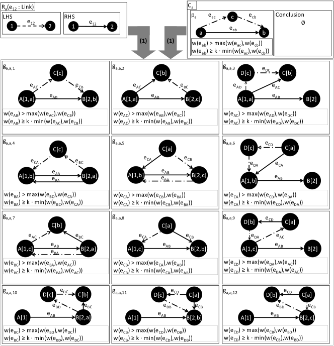
Figure 21: All twelve gluings of the activation rule $R_{\textrm{a}}$ and the active-link constraint $C_{\textrm{a}}$

These gluings are similar to the gluings shown in Figure 20, but the link state constraints are non-conflicting here. In this case, the gluings and their corresponding application conditions can be categorized as follows:

• Unsatisfiable gluings: None of the gluings $g_{\textrm{a},\textrm{a},z\,,\,1\leq z\leq 12}$ is unsatisfiable.

• Restrictive NACs: Gluings $g_{\textrm{a},\textrm{a},1}$, $g_{\textrm{a},\textrm{a},2}$, and $g_{\textrm{a},\textrm{a},8}$ are transformed into three NACs in step (4), as shown in Figure 23.

  

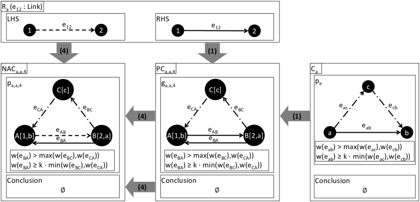
  Figure 22: Transformation of gluing $g_{\textrm{a},\textrm{a},4}$ into the redundant application condition $\text{NAC}_{\textrm{a},\textrm{a},4}$

  For instance, for gluing $g_{\textrm{a},\textrm{a},1}$, applying the activation rule $R_{\textrm{a}}$ in reverse order implies that the link state constraint $\operatorname{s}(e_{\text{AB}})=\texttt{Active}$ is replaced with $\operatorname{s}(e_{\text{AB}})=\texttt{Unclassified}$.

• Redundant NACs: The other nine gluings result in redundant NACs; gluing $g_{\textrm{a},\textrm{a},4}$ serves as a representative example whose transformation is shown in Figure 22:

  

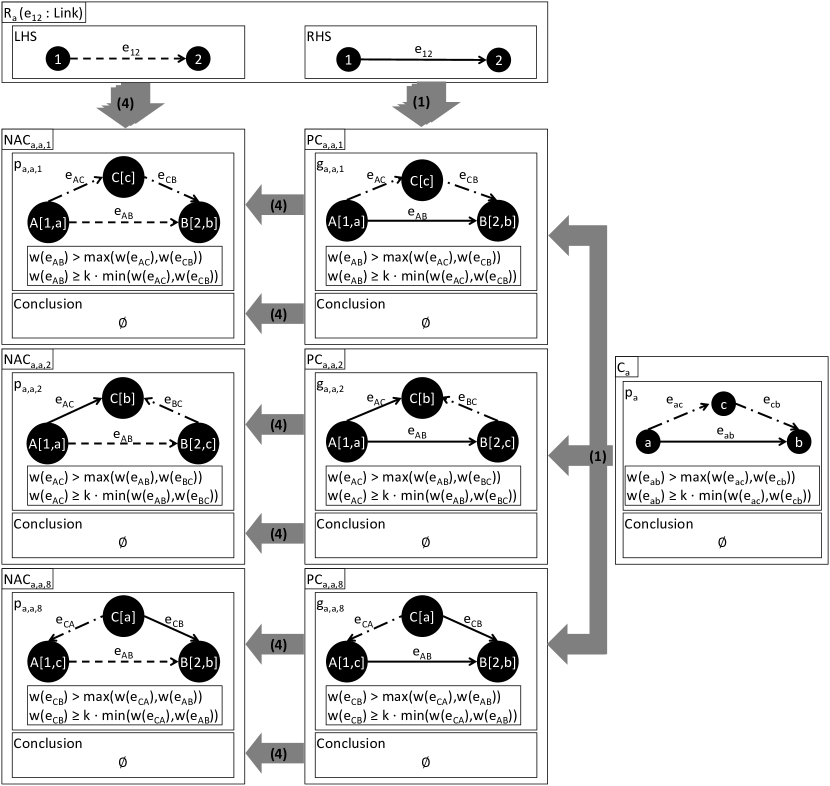
  Figure 23: Transformation of the gluings $g_{\textrm{a},\textrm{a},1}$ $g_{\textrm{a},\textrm{a},2}$, and $g_{\textrm{a},\textrm{a},8}$ into three restrictive NACs of the activation rule $R_{\textrm{a}}$

  The gluing $g_{\textrm{a},\textrm{a},4}$ serves as the premise for the post-condition $\text{PC}_{\textrm{a},\textrm{a},4}$, and the set of conclusions of the post-condition is empty. The application condition is obtained by setting the link state constraint of $e_{\text{AB}}$ to $\operatorname{s}(e_{\text{AB}})=\texttt{Unclassified}$. The additional NAC represents the requirement that the active-link constraint $C_{\textrm{a}}$ must hold for all anti-parallel links of $e_{12}$, whose source node is the target node of $e_{12}$ and vice versa. The constructed application condition is redundant due to the assumption that the topology is weakly consistent prior to applying the activation rule $R_{\textrm{a}}$.

As a result of this refinement step, the three non-redundant new NACs $\text{NAC}_{\textrm{a},\textrm{a},1}$, $\text{NAC}_{\textrm{a},\textrm{a},2}$, and $\text{NAC}_{\textrm{a},\textrm{a},8}$ were added to the activation rule $R_{\textrm{a}}$.

$R_{\textrm{i}}$ + $C_{\textrm{a}}$ The refinement of the inactivation rule $R_{\textrm{i}}$ is similar to the previous case. We obtain $12$ possible gluings $g_{\textrm{i},\textrm{a},z\,,\,1\leq z\leq 12}$ similar to those shown in Figure 21. The major difference is that the link state constraint of $e_{\text{AB}}$ originating from $R_{\textrm{u}}$ is now $\operatorname{s}(e_{\text{AB}})=\texttt{Inactive}$ in all gluings. In this case, the gluings and their corresponding application conditions can be categorized into three groups:

• Unsatisfiable gluing: Gluing $g_{\textrm{i},\textrm{a},1}$ is unsatisfiable due to the conflicting attribute constraints $\operatorname{s}(e_{\text{AB}})=\texttt{Inactive}$ (from $R_{\textrm{i}}$) and $\operatorname{s}(e_{\text{AB}})=\texttt{Active}$ (from $C_{\textrm{a}}$) and is discarded during step (2).

• Restrictive NACs: As before, applying the refinement procedure to the gluings $g_{\textrm{i},\textrm{a},2}$ and $g_{\textrm{i},\textrm{a},8}$ results in two new non-redundant NACs as shown in Figure 24.

• Redundant NACs: As above, the remaining nine gluings correspond to redundant NACs due to the assumption that the topology fulfills the active-link constraint $C_{\textrm{a}}$ prior to any application of the inactivation rule $R_{\textrm{i}}$.

As a result of this refinement step, the two new non-redundant NACs $\text{NAC}_{\textrm{i},\textrm{a},2}$ and $\text{NAC}_{\textrm{i},\textrm{a},8}$ were added to the inactivation rule $R_{\textrm{i}}$.

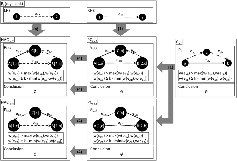
Figure 24: Transformation of the gluings $g_{\textrm{i},\textrm{a},2}$ and $g_{\textrm{i},\textrm{a},8}$ into the restrictive application conditions $\text{NAC}_{\textrm{i},\textrm{a},2}$ and $\text{NAC}_{\textrm{i},\textrm{a},8}$

5.1.5 Refining Context Event Rules to Preserve the Inactive-Link Constraint

After describing the refinement procedure for the TC rules in detail, the corresponding steps for the context event rules in this section are presented in an abbreviated form. Recall that, in general, applying a rule to a topology preserves a positive constraint (i) if all new matches of the premise of the constraint that result from applying the rule may be extended to matches of the conclusion of this constraint, and (ii) if for each existing match of its premise that also exists after the rule application, at least one corresponding match of the conclusion exists.

$R_{\textrm{+n}}$ + $C_{\textrm{i}}$ The node addition rule $R_{\textrm{+n}}$ preserves the inactive-link constraint $C_{\textrm{i}}$ because a rule application of $R_{\textrm{+n}}$ adds an isolated node. Neither a new match of the premise is created nor a match of the conclusion is destroyed by adding a node to the topology. Therefore, the inactive-link constraint $C_{\textrm{i}}$ is already preserved by the node addition rule $R_{\textrm{+n}}$.

$R_{\textrm{-n}}$ + $C_{\textrm{i}}$ The node removal rule $R_{\textrm{-n}}$ preserves the inactive-link constraint $C_{\textrm{i}}$ because a rule application of $R_{\textrm{-n}}$ removes only isolated nodes, which may not be part of a match neither of the premise nor of the conclusion of $C_{\textrm{i}}$.

$R_{\textrm{+e}}$ + $C_{\textrm{i}}$ The link addition rule $R_{\textrm{+e}}$ preserves the inactive-link constraint $C_{\textrm{i}}$ because a rule application of $R_{\textrm{+e}}$ adds an unclassified link to a topology. Adding an unclassified link neither produces a match of the premise of $C_{\textrm{i}}$ that cannot be extended to a match of the conclusion nor destroys any match of the conclusion of $C_{\textrm{i}}$.

$R_{\textrm{-e}}$ + $C_{\textrm{i}}$ The link removal rule $R_{\textrm{-e}}$ does not preserve the inactive-link constraint $C_{\textrm{i}}$ because a match of the conclusion may be destroyed without destroying the corresponding match of the premise. The refinement procedure of the link removal rule $R_{\textrm{-e}}$ and the inactive-link constraint $C_{\textrm{i}}$ proceeds completely analogous to the refinement procedure of the unclassification rule $R_{\textrm{u}}$ and the inactive-link constraint $C_{\textrm{i}}$. For brevity, we only present the resulting refined link removal rule $R_{\textrm{-e}}$ in Figure 25. Note that the premises of the application conditions only match if the link $e_{12}$ is either active or inactive and if it has an incident inactive link.

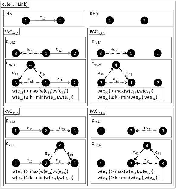
Figure 25: Final refined link removal rule $R_{\textrm{-e}}$

$R_{\textrm{mod-w}}$ + $C_{\textrm{i}}$ The weight modification rule $R_{\textrm{mod-w}}$ may violate the inactive-link constraint $C_{\textrm{i}}$ in the very same way as the link removal rule $R_{\textrm{-e}}$ does. Therefore, we omit the details of the derivation of the application conditions and only present the refined unclassification rule $R_{\textrm{u}}$ in Figure 26. One particularity here is the attribute constraint that requires $\operatorname{w}(e_{\text{12}})$ to equal $w_{\text{new}}$ after applying $R_{\textrm{mod-w}}$. This attribute constraint is still present in the gluings that yield the post-conditions (not shown here), but it is missing from the resulting application conditions $\text{PAC}_{\textrm{mod-w},\textrm{i},2}$, $\text{PAC}_{\textrm{mod-w},\textrm{i},4}$, $\text{PAC}_{\textrm{mod-w},\textrm{i},5}$, and $\text{PAC}_{\textrm{mod-w},\textrm{i},6}$ because applying $R_{\textrm{mod-w}}$ in reverse order removes this attribute constraint.

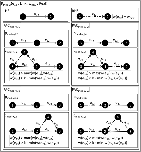
Figure 26: Final refined weight modification rule $R_{\textrm{mod-w}}$

5.1.6 Refining Context Event Rules to Preserve the Active-Link Constraint

As in the previous iteration, we abbreviate the description of the application of the refinement procedure in the following. Recall that applying a rule to a topology preserves a negative constraint if the rule application may not produce any new matches of the premise of the constraint.

$R_{\textrm{+n}}$ + $C_{\textrm{a}}$ The node addition rule $R_{\textrm{+n}}$ preserves the active-link constraint $C_{\textrm{a}}$ because an application of $R_{\textrm{+n}}$ adds an isolated node and, therefore, never produces a new match of the premise of $C_{\textrm{a}}$.

$R_{\textrm{-n}}$ + $C_{\textrm{a}}$ The node removal rule $R_{\textrm{-n}}$ preserves the active-link constraint $C_{\textrm{a}}$ because a rule application of $R_{\textrm{-n}}$ removes an isolated node and, therefore, never produces a new match of the premise of $C_{\textrm{a}}$.

$R_{\textrm{+e}}$ + $C_{\textrm{a}}$ The link addition rule $R_{\textrm{+e}}$ preserves the active-link constraint $C_{\textrm{a}}$ because a rule application of $R_{\textrm{+e}}$ adds an unclassified link to a topology, which may never produce a new match of the premise of $C_{\textrm{a}}$.

$R_{\textrm{-e}}$ + $C_{\textrm{a}}$ The link removal rule $R_{\textrm{-e}}$ preserves the active-link constraint $C_{\textrm{a}}$ because a rule application of $R_{\textrm{-e}}$ removes a link and, therefore, never produces a new match of the premise of $C_{\textrm{a}}$.

$R_{\textrm{mod-w}}$ + $C_{\textrm{a}}$ The weight modification rule $R_{\textrm{mod-w}}$ preserves the active-link constraint $C_{\textrm{a}}$ because a rule application of $R_{\textrm{mod-w}}$ unclassifies a link, which cannot result in a new match of the premise of $C_{\textrm{a}}$.

Intermediate Summary

After applying the refinement procedure to all combinations of GT rules and kTC-specific constraints, all refined rules preserve weak consistency. Figure 27 shows the specification of the kTC algorithm after Section 5.1. The output topology fulfills the unclassified-link constraint $C_{\textrm{u}}$ because the stop node is only reached if the topology contains no more unclassified links.

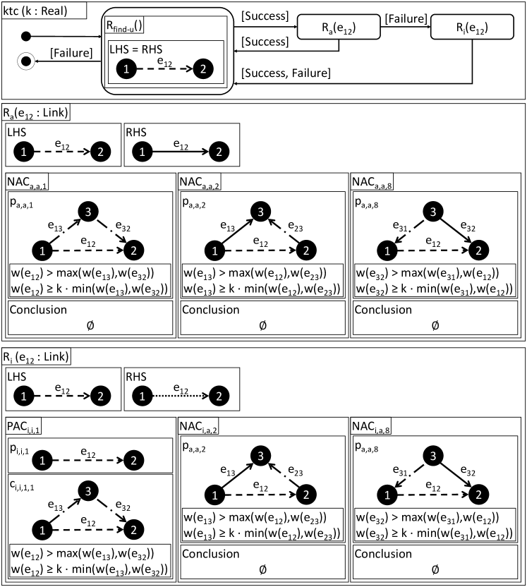
Figure 27: GT operation ktc, the specification of kTC after rule refinement in Section 5.1

5.2 Restoring Applicability of Unrestrictable Rules via Handler Operations

Section 5.1 resulted in additional application constraints for three unrestrictable GT rules: the unclassification rule $R_{\textrm{u}}$, the link removal rule $R_{\textrm{-e}}$, and the weight modification rule $R_{\textrm{mod-w}}$. The weight modification rule $R_{\textrm{mod-w}}$, for instance, is currently only applicable if the resulting topology is still weakly consistent. As explained in Section 2.3, unrestrictable GT rules represent (voluntarily or involuntarily) non-controllable modifications of the topology. Therefore, the goal of this section is to restore the applicability of all unrestrictable GT rules (G2), but without sacrificing the guarantee that applying any of the unrestrictable rules preserves weak consistency (G1).

The following proposed solution is one of the main contributions of this paper. We suggest to systematically turn any added application condition $\text{AC}_{x,y}$ of an unrestrictable GT rule $R_{x}$ into appropriate restoration operations restore-$\text{AC}_{x,y}$. The purpose of this restoration operation is to resolve any violations of weak consistency caused by not checking $\text{AC}_{x,y}$.

Figure 28 shows the general idea of deriving restoration operations from application conditions of a GT rule $R_{x}$: Each application of $R_{x}$ is replaced with a corresponding handler operation handle-$R_{x}$.

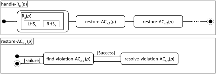
Figure 28: Schematic overview of derivation of restoration operations

For each application condition $\text{AC}_{x,y}$ to be dropped, a restoration operation restore-$\text{AC}_{x,y}$ is invoked after applying $R_{x}$. The restoration operation restore-$\text{AC}_{x,y}$ iteratively identifies all violations of $\text{AC}_{x,y}$ by means of a violation identification operation and resolves the identified violation by means of a violation resolution operation. A restoration operation terminates only if all constraint violations have been eliminated. In the schematic overview shown in Figure 28, we assume that $R_{x}$ takes a (potentially empty) list $p$ of parameters (e.g., the link variable $e_{\text{12}}$ of $R_{\textrm{u}}$). The corresponding handler operation handle-$R_{x}$ has the same list of parameters p as $R_{x}$. The parameter list p is forwarded to $R_{x}$ and the restoration operations restore-$\text{AC}_{x,y}$. The following properties have to be proved for each restoration operation.

• The resolution of a particular constraint violation should not result in new constraint violations at the affected match of $R_{x}$. Otherwise, the restoration operation may not terminate. Still, it may be necessary to create constraint violations either of other application conditions or at a different match of the current application condition. Such violations have to be handled subsequently (e.g., by recursively invoking restoration operations).

• A general assumption in our scenario is that constraint violations can be resolved by unclassifying links. This is a valid assumption because the application conditions were derived from the constraints of weak consistency. Weak consistency is guaranteed to hold on a completely unclassified topology (see Theorem 4). Therefore, a naïve violation resolution operation could simply unclassify all links in the topology.

Table 4: Overview of operations introduced during the restoration step (Section 5.2)

Conventional Name	Description
handle-$R_{x}$	Handler operation for $R_{x}$, which ensures that weak consistency is preserved when applying the unrestricted version of $R_{x}$
restore-$\text{AC}_{x,y}$	Restoration operation for $\text{AC}_{x,y}$, which restores application condition $\text{AC}_{x,y}$ by eliminating all violations of $\text{AC}_{x,y}$ that result from applying $R_{x}$
find-violation-$\text{AC}_{x,y}$	Violation identification operation for $\text{AC}_{x,y}$, which identifies some violation of $\text{AC}_{x,y}$
resolve-violation-$\text{AC}_{x,y}$	Violation resolution operation for $\text{AC}_{x,y}$, which resolves a given violation of $\text{AC}_{x,y}$

In the following subsections, we illustrate the concrete derivation of violation identification and resolution operations, based on affected rules $R_{\textrm{u}}$, $R_{\textrm{-e}}$, and $R_{\textrm{mod-w}}$.

5.2.1 Deriving Repair Operations for the Unclassification Rule

Applying the refinement algorithm to the unclassification rule $R_{\textrm{u}}$ resulted in four additional application conditions—$\text{PAC}_{\textrm{u},\textrm{i},2}$, $\text{PAC}_{\textrm{u},\textrm{i},4}$, $\text{PAC}_{\textrm{u},\textrm{i},5}$, and $\text{PAC}_{\textrm{u},\textrm{i},6}$—as shown in Figure 17. These application conditions essentially require that the affected link $e_{\text{12}}$ may only be inactivated if each incident inactive link of the source and target node of the affected link can be extended to a triangle that matches the conclusion of the inactive-link constraint $C_{\textrm{i}}$.

Figure 29 shows the handler operation handle-$R_{\textrm{u}}$ and one restore-$\text{PAC}_{\textrm{u},\textrm{i},2}$.

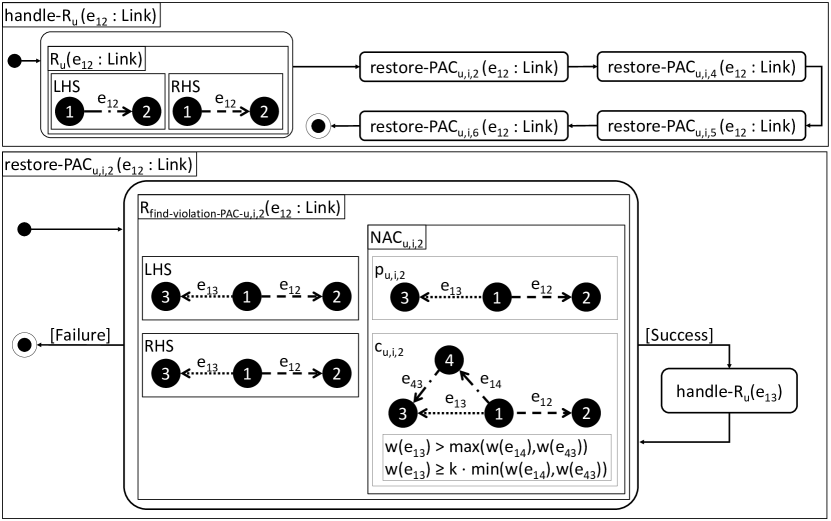
Figure 29: Handler operation handle-$R_{\textrm{u}}$ for unclassification rule $R_{\textrm{u}}$

The parameter list of $R_{\textrm{u}}$ contains one link variable $e_{\text{12}}$. Corresponding to the four application conditions, we create four restoration operations: restore-$\text{PAC}_{\textrm{u},\textrm{i},2}$, restore-$\text{PAC}_{\textrm{u},\textrm{i},4}$, restore-$\text{PAC}_{\textrm{u},\textrm{i},5}$, and restore-$\text{PAC}_{\textrm{u},\textrm{i},6}$. For conciseness, we only show and discuss the first restoration rule, restore-$\text{PAC}_{\textrm{u},\textrm{i},2}$. The violation identification operation of $\text{PAC}_{\textrm{u},\textrm{i},2}$ consists of the sole rule $R_{\text{find-violation-}\text{PAC}_{\textrm{u},\textrm{i},2}}$ and is, therefore, inlined here. This rule essentially identifies some inactive link $e_{\text{13}}$ for which $e_{\text{12}}$ is part of the sole match of the conclusion of the inactive-link constraint $C_{\textrm{i}}$. To identify such situations, the positive application condition $\text{PAC}_{\textrm{u},\textrm{i},2}$ is turned into the negative $\text{NAC}_{\textrm{u},\textrm{i},2}$ of $R_{\text{find-violation-}\text{PAC}_{\textrm{u},\textrm{i},2}}$. For each identified link $e_{\text{13}}$, unclassifying $e_{\text{12}}$ would result in a violation of $\text{PAC}_{\textrm{u},\textrm{i},2}$—and thereby of $C_{\textrm{u}}$—if no countermeasures are taken because the sole match of the conclusion of $\text{PAC}_{\textrm{u},\textrm{i},2}$ at $e_{\text{13}}$ would be destroyed.

To resolve the identified, immanent constraint violation at $e_{\text{13}}$, we apply the default violation resolution strategy and unclassify $e_{\text{13}}$ in this case. A more sophisticated strategy could try to establish an additional match of the conclusion of $C_{\textrm{i}}$, e.g., by classifying other links appropriately. While this strategy is certainly a means to reduce the number of links that need to be unclassified, it is not generally applicable because we may easily come up with topologies that, for instance, do not contain alternate triangles. Therefore, we chose the default strategy here, which means that the violation resolution operation is a recursive call to handle-$R_{\textrm{u}}$ with the problematic link variable $e_{\text{13}}$ as parameter. The restoration operations for the other three ACs ($\text{PAC}_{\textrm{u},\textrm{i},4}$, $\text{PAC}_{\textrm{u},\textrm{i},5}$, and $\text{PAC}_{\textrm{u},\textrm{i},6}$) are derived in an analogous manner.

The recursive invocation of handle-$R_{\textrm{u}}$ is guaranteed to terminated. The reason is that, at each invocation of handle-$R_{\textrm{u}}$, at least one classified link is being unclassified by invoking $R_{\textrm{u}}$ prior to the recursive invocations of handle-$R_{\textrm{u}}$.

5.2.2 Deriving Repair Operations for the Context Event Rules

Steps for deriving restoration operations for the link removal rule $R_{\textrm{-e}}$ and the weight modification rule $R_{\textrm{mod-w}}$ are completely analogous to the steps for the unclassification rule $R_{\textrm{u}}$ and are, therefore, omitted for brevity.

5.2.3 Context Event Rules and Connectivity

A crucial assumption of our approach is that the topology is weakly consistent whenever ktc is invoked, i.e., ktc is designed to preserve weak consistency, not to enforce it. Between two invocations of ktc, an arbitrary number of context events may occur. After the modifications to the context event rules described in this section, we may safely assume that an appropriate restoration operation is invoked whenever a context event occurs. Based on this assumption, we can prove the following theorem.

Theorem 8

The refined context event rules preserve weak connectivity on physically connected topologies.

Sketch of proof. The refined context event rules (with the restoration operations) preserve weak consistency. According to Theorem 6, weak consistency implies weak connectivity; therefore, the claim follows.

5.3 Enforcing Termination of ktc via Handler Operations

In this section, we first illustrate that the current version of ktc (shown in Figure 27) may run into situations that lead to an infinite execution in Section 5.3.1. Based on these observations and the concept of restoration operations, as described in Section 5.2, we introduce a pre-processing operation that ensures that one of the two TC rules, $R_{\textrm{a}}$ or $R_{\textrm{i}}$, is applicable in each iteration of the TC algorithm. This step fulfills goal G3.

5.3.1 Example of Non-Termination and Problem Analysis

As Figure 30(a) shows, there are topologies for which the current TC algorithm may not terminate: Starting with an entirely unclassified topology, the TC algorithm activates $e_{23}$ and inactivates $e_{13}$. Now, the unclassified link $e_{12}$ may be neither activated nor inactivated because the activation rule $R_{\textrm{a}}$ and the inactivation rule $R_{\textrm{i}}$ share two pairs of NACs that may prevent the applicability of both TC rules in this situation. In general, if $\text{NAC}_{\textrm{a},\textrm{a},2}$ prevents the application of $R_{\textrm{a}}$ for a certain unclassified link, then $\text{NAC}_{\textrm{i},\textrm{a},2}$ also prevents the application of $R_{\textrm{i}}$. The same holds for $\text{NAC}_{\textrm{a},\textrm{a},8}$ and $\text{NAC}_{\textrm{i},\textrm{a},8}$, respectively.

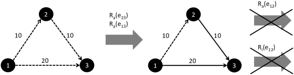
(a) Initial situation

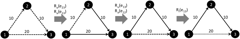
(b) Possible solution: re-unclassifying weight-maximal link $e_{13}$

Figure 30: Example of non-termination of ktc (Figure 27) and a possible solution

Figure 30(b) depicts a possible solution for this particular situation: When processing the unclassified link $e_{12}$, the wrong classification of link $e_{13}$ is reverted by unclassifying $e_{13}$. Afterwards, the activation rule $R_{\textrm{a}}$ is successfully applied to link $e_{12}$, leaving only one unclassified link, $e_{13}$, which finally gets inactivated. The preceding discussion shows that (i) processing links in an “unfavorable” order may cause wrong classifications, and (ii) at least two possible solutions to this problem exist.

As a first solution, we could pre-determine the order of processing of the unclassified links to ensure that less (or even no) unclassifications are necessary. Currently, the processing order is non-deterministic: the unclassified-link identification rule $R_{\textrm{find-u}}$ may return any of the unclassified links in the topology. Pre-determining the processing order brings the benefit of no or few required re-classifications of links, but it may be non-trivial to identify such a suitable link processing order.

As a second solution, we could re-unclassify links whose state is known to be “wrong.” In the case of kTC, “wrong” means that a particular link blocks the activation and inactivation of an unclassified link. This solution brings the benefit that the processing order needs not be pre-determined, leaving this decision to the underlying GT engine or code generator that executes the GT rules. The downside is that links may be re-unclassified many times if the re-unclassification logic is not properly specified.

5.3.2 Introducing Handler Operations

We propose to apply the second solution for the kTC case study. We take the very same approach as in Section 5.2: Our goal is to eventually drop two critical pairs of negative application conditions: $\text{NAC}_{\textrm{a},\textrm{a},2}$ and $\text{NAC}_{\textrm{i},\textrm{a},2}$ plus $\text{NAC}_{\textrm{a},\textrm{a},8}$ and $\text{NAC}_{\textrm{i},\textrm{a},8}$. To this end, we treat these ACs in the same way as the additional ACs of the unrestrictable rules: We may replace the application of the activation rule $R_{\textrm{a}}$ and the inactivation rule $R_{\textrm{i}}$ with invocations of appropriate handler operations. In handle-$R_{\textrm{a}}$, we may then introduce the restoration operations restore-$\text{NAC}_{\textrm{a},\textrm{a},2}$ and restore-$\text{NAC}_{\textrm{a},\textrm{a},8}$, and in handle-$R_{\textrm{i}}$, we may then introduce the restoration operations restore-$\text{NAC}_{\textrm{i},\textrm{a},2}$ and restore-$\text{NAC}_{\textrm{i},\textrm{a},8}$. The remaining ACs—$\text{PAC}_{\textrm{i},\textrm{i},1}$ and $\text{NAC}_{\textrm{a},\textrm{a},1}$—are considered later.

This time, however, we proceed slightly differently, achieving the same result but with improved performance and readability: Instead of inserting a restoration operation for each of the two affected rules, we only invoke the restoration operation once prior to applying the first rule ($R_{\textrm{a}}$ in this case). This is valid because the derived restoration operations would be identical for both rules, and no new constraint violations may be created by invoking the activation rule $R_{\textrm{a}}$, because the inactivation rule $R_{\textrm{i}}$ is only tried if the first rule application has failed.

Figure 31 depicts the resulting, and final, version of the operation ktc, the additional handler operation, and the activation rule $R_{\textrm{a}}$ and inactivation rule $R_{\textrm{i}}$ after removing the NACs that are now always fulfilled. The handler operation consists of two loops that unclassify the weight-maximal links $e_{13}$ and $e_{23}$ in each match of the premise of corresponding NACs. For each unclassification of an active link $e_{13}$/$e_{32}$, the repair operation repair-u of the unclassification rule $R_{\textrm{u}}$ (as shown in Figure 29) is invoked to repair possible constraint violations.

Note that the premise of $\text{NAC}_{\textrm{a},\textrm{a},1}$ and the conclusion of $\text{PAC}_{\textrm{i},\textrm{i},1}$ are equivalent, i.e., each match of $\text{NAC}_{\textrm{a},\textrm{a},1}$ is also a match of $\text{PAC}_{\textrm{i},\textrm{i},1}$. This means that the activation rule $R_{\textrm{a}}$ in Figure 31 is applicable to a given link $e_{12}$ if and only if the inactivation rule $R_{\textrm{i}}$ is not applicable to the same link. For this reason, we could remove $\text{PAC}_{\textrm{i},\textrm{i},1}$ from $R_{\textrm{i}}$ for performance and readability reasons.

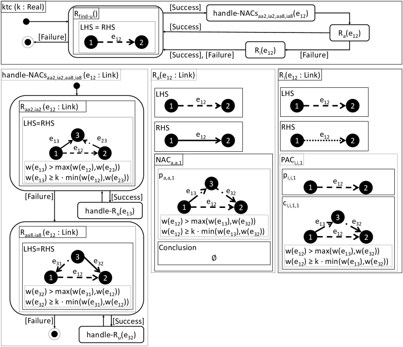
Figure 31: GT operation ktc, the final specification of kTC after enforcing termination in Section 5.3

5.3.3 Proof of Termination

After showing that the TC algorithm produces strongly consistent topologies, which fulfill the active-link constraint $C_{\textrm{a}}$, the inactive-link constraint $C_{\textrm{i}}$, and the unclassified-link constraint $C_{\textrm{u}}$, it remains to show that the TC algorithm, shown in Figure 31, terminates.

Theorem 9 (Termination)

ktc terminates for any input topology.

Proof. We have to show that the number of rule applications of the unclassified-link identification rule $R_{\textrm{find-u}}$ is finite for any input topology. Consider a topology with link set $E$. We consider the sequence of all link states $s_{i}(e_{1}),\ldots,s_{i}(e_{m})$ with $m:=|E|$ after the $i$-th execution of $R_{\textrm{find-u}}$, where the links are ordered according to their weight:

$$\forall v,w\in\{1,\dots,m\}:\operatorname{w}(e_{v})<\operatorname{w}(e_{w})\Rightarrow v<w$$

Note that the right-to-left implication does not hold because no order is imposed on two links $e_{v}$, $e_{w}$ that have an identical weight value. We compare two sequences of link states, $s_{i}$ and $s_{j}$, as follows: $s_{i}\prec s_{j}$ if and only if (i) some link $e_{v}$ is unclassified in $s_{i}$ and active or inactive in $s_{j}$, and (ii) the states of all links with a weight less than $e_{v}$ are identical in $s_{i}$ and $s_{j}$, formally:

$$s_{i}\prec s_{j}\;:\Leftrightarrow\; \exists v\in\{1,\dots,m\}:s_{i}(e_{v})=\texttt{Unclassified}\;\wedge\;s_{j}(e_{v})\in\{\texttt{Active},\texttt{Inactive}\}$$

$$\wedge\forall w\in\{1,\dots,v-1\}:s_{i}(e_{w})=s_{j}(e_{w})$$

Note that any sequence that consists of active and inactive links only is an upper bound for $\prec$.

We now show that $s_{i-1}\prec s_{i}$ for $i>1$. Let $e_{v}$ be the link that is bound by applying the unclassified-link identification rule $R_{\textrm{find-u}}$. The pre-processing operation unclassifies only links $e_{w}$ if $\operatorname{w}(e_{w})>\operatorname{w}(e_{v})$ with $w>v$. The activation rule $R_{\textrm{a}}$ or the inactivation rule $R_{\textrm{i}}$ activate or inactivate $e_{v}$, respectively.

Therefore, $s_{i-1}\prec s_{i}$ because (i) the first $v{-}1$ elements of $s_{i-1}$ and $s_{i}$ are identical, and (ii) $s_{i-1}(e_{w})=\texttt{Unclassified}$and $s_{i}(e_{w})\in\{\texttt{Active},\texttt{Inactive}\}$. The termination follows because any ordered sequence $s_{1}\prec s_{2}\prec\dots$ has a finite length.

Example

To illustrate the comparison of link state sequences, Table 5 shows the link state sequences for the previous example in Figure 30(b). The columns are sorted by increasing weight. In the third iteration, the pre-processing operation unclassifies $e_{13}$, which ensures that the activation rule $R_{\textrm{a}}$ may be applied to $e_{12}$.

Table 5: Link states after each iteration of the example in Figure 30(b)

.

Iteration	State after Iteration
	$\operatorname{s}(e_{12})$	$\operatorname{s}(e_{23})$	$\operatorname{s}(e_{13})$
(initial)	Unclassified	Unclassified	Unclassified
1	Unclassified	Active	Unclassified
2	Unclassified	Active	Active
3	Active	Active	Unclassified
4	Active	Active	Inactive

This proof concludes the refinement of the TC rules. We have shown that the refined rules preserve the active-link constraint $C_{\textrm{a}}$ and the inactive-link constraint $C_{\textrm{i}}$ and that introducing the pre-processing operation enforces the termination of the TC algorithm.

5.4 Summary of Rule Refinement

We conclude this section with a short overview of its results. First, to ensure that the TC and context event rules preserve weak consistency (G1), we first applied the constructive approach by Heckel and Wagner [42] in Section 5.1. Then, we introduced the complementary restoration step in Section 5.2. This step is necessary to fulfill the goal that the unrestrictable GT rules—the unclassification rule $R_{\textrm{u}}$ and the context event rules—should always be applicable (G2). The restoration step systematically transforms all additional application conditions into restoration operations that eliminate (anticipated) constraint violations caused by applying the original GT rules. Finally, we observed that an unfavorable processing order of unclassified links may lead to a non-termination of ktc, which contradicts goal G3. We solved this problem by re-using the concept of restoration operations: We transformed the problematic application conditions into appropriate restoration operations. Thereby, we enforced the applicability of at least one of the TC rules in each iteration of the TC algorithm.

6 Simulation-Based Evaluation

In this section, we evaluate the incremental specification of kTC constructed in Section 5. For this evaluation, we use the GT tool eMoflon [23] to automatically transform the specification of kTC into executable Java code. For simulating WSNs, we use the network simulation platform Simonstrator [61].

In Section 6.1, we present the research questions to be answered during this evaluation. In Section 6.2, we outline the evaluation setup. In Sections 6.3, 6.4, 6.6 and 6.5, we present and discuss the results to answer the four identified research questions. In Section 6.7, we discuss threats to validity and summarize the results of the evaluation.

6.1 Research Questions

We emphasize that the focus of this paper is not to develop a new TC algorithm but to derive a novel, incremental version of an established TC algorithm using the correct-by-construction approach presented in the preceding sections. Therefore, the following research questions focus on the general validity, applicability, and performance of our approach. Our goal is not to perform a detailed analysis of the TC algorithm w.r.t. network-specific metrics (e.g., network lifetime, energy consumption). The answers to the following research questions are summarized in Table 11 at the end of this section.

RQ1–Correctness: The implementation that is derived from the GT-based specification should always be correct. The implementation is correct if the topology is always weakly consistent and if ktc always terminates and returns a strongly consistent topology. More specifically, in Section 6.3, we will address the following questions:

• Is the topology always weakly consistent after context event handling?

• Does ktc always terminate? Is the resulting topology strongly consistent?

RQ2–Incrementality: Incrementality is an fundamental property of the TC algorithms developed using our approach. We quantitatively assess incrementality in terms of the number of link state modifications required to handle context events and to re-optimize the topology. More specifically, in Section 6.4, we will address the following questions:

• Which properties of a topology (e.g., node count, node density) influence the cost of handling context events and invoking TC?

• How large is the cost of executing incremental kTC compared to batch kTC?

RQ3–Performance: From a practical perspective, it is crucial that simulations may be performed in sensible time. While we only have limited influence on the execution time of the actual simulation (e.g., due to simulated network traffic), the overhead of executing ktc should remain reasonable. The purpose of this research question is to evaluate this overhead quantitatively. More specifically, in Section 6.5, we will address the following questions:

• What fraction of execution time is spent on executing ktc?

• Is the total execution time of ktc sensible for topologies of realistic size?

RQ4–Generalizability: The proposed methodology shall help reducing the gap between specification and implementation that is pertinent in the WSN community. This research question addresses the general applicability of the proposed approach. More specifically, in Section 6.6, we will discuss the following questions:

• Is meta-modeling suitable to specify all relevant properties of WSN topologies?

• Are GT rules suitable to specify context events and TC operations?

• Are graph constraints and the proposed refinement algorithm suitable to specify and ensure the preservation of consistency constraints and optimization goals of typical TC algorithms?

• Is a TC developer able to apply the described methodology?

6.2 Evaluation Setup

Following best practice for simulation studies (e.g., [62, 63]), we document the evaluation setup in detail to foster reproducibility of our results. The technical platforms of this evaluation are the GT tool eMoflon [23] and the network evaluation platform Simonstrator [61] with its contained network simulator PeerfactSim.KOM [64], as shown in Figure 32 and as described in detail in the following.

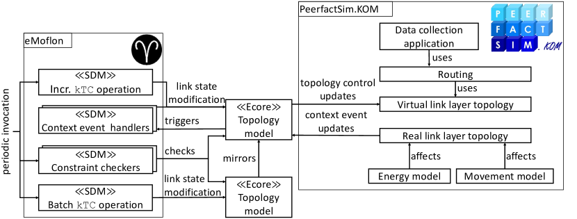
Figure 32: Overview of the evaluation setup

eMoflon

The context event handlers and the GT operation ktc have been specified using a visual syntax of story diagrams in eMoflon. The specification is compiled into EMF-compliant Java code, which operates on an EMF-based topology model. The topology meta-model has been specified in Ecore [65]. Whenever the topology model is modified by a context event in the simulator, the corresponding handler operation is triggered. The TC algorithm ktc periodically updates the topology model via link state modifications.

Simulator

PeerfactSim.KOM [64] is a time-discrete network simulator that allows to simulate protocols on the underlay (i.e., the physical and link layer of the ISO-OSI reference model [66]) as well as on the overlay (i.e., network, transport and application layer [66]).

Topology control via virtual topologies

Upper-layer protocols typically operate on the topology view provided by lower-layer protocols. We created a generic topology framework that introduces virtual topologies: The virtual topology is a view of the corresponding real topology, which is used by upper-layer applications instead of the real topology. In this evaluation, we consider the real and virtual link layer topology. Using a virtual link layer topology allows us to apply TC transparently, i.e., without the upper-layer protocols noticing that they operate on a modified view of the real topology. The real link layer topology is affected by two types of context events:

• The energy model of a node simulates the depletion of its battery over time. The energy model determines the initial charge of the battery and the amount of energy that transmitting a message of a certain size requires. We say that a node is alive at a certain point in time if its battery is not empty.

• The movement model specifies the movement of each node inside the bounds of the simulation area. In this scenario, we use a modified version of the Gauss-Markov movement model [67]. To simulate the typically low dynamics in WSNs, we introduced a hesitation probability of $99\text{\,}\mathrm{\char 37\relax}$: This is the probability that a node does not move within a time step. Node movement causes link weight modifications and link additions/removals if one node enters/leaves another node’s transmission range.

The modifications of the topology model caused by context events trigger the corresponding handler operations. In the reverse direction, link state modifications of the topology model that result from an invocation of ktc are propagated to the virtual link layer topology. The virtual link layer topology contains all links in the original link layer topology that are either active or unclassified, which ensures that the link layer topology remains connected even in the presence of context events.

In this evaluation, TC is invoked periodically every $10\text{\,}\mathrm{min}$ (simulation time). The parameter $k$ of kTC is set to 1.41, which is a typical value [68]. The set of context events is collected during this period and handled prior to invoking TC. We subsume the subsequent execution of context event handling and TC invocation under the term TC run, i.e., every $10\text{\,}\mathrm{min}$, a TC run is performed.

Overlay

On top of the virtual link layer topology, a typical (many-to-one) data collection application [69] is running: All sensor nodes periodically send data messages to a central base station node, which has a fixed power supply (modeled using a very large battery capacity of $100\text{\,}\mathrm{kJ}$). The transmitted messages are routed by a global knowledge routing algorithm, which operates on the complete virtual link layer topology.

Table 6 summarizes the parameters of the simulation setting that are fixed for all configurations. We run each simulation in terminating mode, i.e., we abort the simulation after $20\text{\,}\mathrm{h}$, regardless of the remaining number of alive nodes. This means that, in each simulation run, TC is performed $\frac{$20\text{\,}\mathrm{h}$}{$10\text{\,}\mathrm{min}$}-1=\numprint{119}$ times because we neglect the initial TC run (at $10\text{\,}\mathrm{min}$ of simulated time) for technical reasons. All experiments were performed on a 64-bit machine with an Intel i7-2600 CPU ($2\text{\,}\mathrm{c}\mathrm{o}\mathrm{r}\mathrm{e}\mathrm{s}$, $3.7\text{\,}\mathrm{GHz}$) and $8\text{\,}\mathrm{GB}$ of RAM running Windows 7 Professional.

Table 6: Common parameter values of all simulation configurations

Parameter	Value
Simulation
Network simulator	PeerfactSim.KOM/ Simonstrator 2.4 [61]
GT-tool	eMoflon 2.15.0 [23]
Number of runs per configuration	15
Seeds	1…15
Simulation type	terminating (after $20\text{\,}\mathrm{h}$ of simulated time)
Measurements per run	119
Code availability	as SHARE virtual machine [70]
World size	variable (see Table 7)
Node configuration
Source node count (initial)	variable (see Table 7)
Target node count	1
Transmission radius	$131\text{\,}\mathrm{m}$
Movement model	Gauss-Markov [67] with hesitation ($p=$99\text{\,}\mathrm{\char 37\relax}$$)
Placement model	uniform at random
Initial battery level (sources)	$130\text{\,}\mathrm{J}$
Initial battery level (target)	$100\text{\,}\mathrm{kJ}$
Link layer and topology control
Link count (initial)	variable (see Table 7)
Link layer	IEEE 802.11 Ad-Hoc
TC algorithm	incremental kTC
$w$ calculation	Euclidean distance between incident nodes
$k$ parameter	1.41
Interval of TC runs	$10\text{\,}\mathrm{min}$
TC runs per simulation run	119
Overlay
Application	Data collection
Communication pattern	many-to-one
Routing	Global knowledge
Message size	$1\text{\,}\mathrm{kB}$
Message transmission frequency	1 message every $10\text{\,}\mathrm{s}$

To obtain a set of (evaluation) configurations, we vary the node count of the initial topology as well as the side length of the quadratic area onto which the nodes are distributed uniformly at random. In total, we investigate six different evaluation configurations, summarized in Table 7, that result from varying the initial node count $n\in\{100,1000\}$ and the world size $w\in\{$750\text{\,}\mathrm{m}$,$500\text{\,}\mathrm{m}$,$250\text{\,}\mathrm{m}$\}$ for $n=100$ and $w\in\{$2000\text{\,}\mathrm{m}$,$1000\text{\,}\mathrm{m}$,$1500\text{\,}\mathrm{m}$\}$ for $n=1000$. Each configuration is simulated 15 times to obtain representative results. In the table, the configurations are ordered from the smallest and sparsest initial topology (n100w750) to the largest and densest topology (n1000w1000).

Table 7: Variable parameters in the six evaluation configurations ($n$: initial node count, $m$: initial link count in real link layer, $w$: side length of quadratic simulation area, $h$: average hop count to base station, $d_{\text{out}}$: average out-degree, values of $m$, $h$, and $d_{\text{out}}$ are averaged over all 15 repetitions)

ID	$n$	$w$ [m]	$m$	$h$	$d_{\text{out}}$
n100w750	100	750	812	3.6	7.7
n100w500	100	500	1 651	2.1	16.0
n100w250	100	250	5 161	1.2	51.2
n1000w2000	1 000	2 000	12 683	7.8	12.1
n1000w1500	1 000	1 500	22 092	5.5	21.6
n1000w1000	1 000	1 000	48 072	3.6	47.5

The node (out-)degree $d_{\text{out}}$ is an indicator of the density of the topology: A high node degree indicates that a topology is dense, while a low node degree indicates a sparse topology. The initial topology of the two sparsest topologies is physically disconnected in 3 out of 15 simulation runs for n100w250 and 1 out of 15 simulation runs for n1000w2000. The lack of connectivity is not a problem because the topology (i) may become physically connected due to node movements and (ii) will eventually become physically disconnected as soon as more and more nodes run out of energy. The average hop count $h$ to the base station is an indicator of the extent of the considered topology.

Batch kTC

This evaluation shall illustrate benefits of incremental TC compared to batch TC. For this reason, we also implemented batch kTC using SDM, which operates on a separate topology model that mirrors the structure of the topology model that is modified by incremental kTC. Prior to each application of batch kTC, all links in the mirrored topology are being unclassified. In the following, we will refer to the incremental and batch variants of kTC as i-kTC and b-kTC, respectively.

6.3 RQ1–Correctness

A central contribution of our approach is that the derived TC algorithms and context event handlers are correct by construction. Recall that correctness means that (i) the TC algorithm always terminates and produces strongly consistent output topologies for weakly consistent input topologies, and (ii) the context event handlers preserve weak consistency. Evidently, this property only holds if all steps of the methodology are performed correctly. Table 8 summarizes steps in the methodology where correctness of the derived TC algorithm and context event handlers may be corrupted, and it shows the steps that we took to mitigate or eliminate these problems.

Table 8: Threats to correctness and applied mitigation strategies (RQ1)

Step	Potential Threat	Mitigation Strategy
Constraint specification (Section 3)	The constraints do not represent the intended objective.	We chose the well-established kTC algorithm, which has already proved to achieve energy savings in a testbed evaluation [71], and carefully translated its basic ideas into graph constraints.
Rule refinement (Section 5.1)	The derived application conditions fail to preserve the specified graph constraints.	The translation of graph constraints into application conditions is theoretically correct, but has been performed by hand for this evaluation, which may not be accurate. To increase confidence in our implementation, the graph constraints that constitute weak and strong consistency are checked during simulation after context event handling and TC invocation, respectively. The large number of context events and TC invocations during the simulation serve as test suite for the implementation. To mitigate the potential errors of performing the manual translation, an automatic derivation of the application conditions would be possible.
Derivation of context event handlers (Section 5.2)	The context event handlers fail to eliminate all possible violations of their original application conditions.	The check of weak consistency after every context event handling serves increases the confidence in the derived handlers.
Code generation (Section 6)	The generated Java code fails to implement the GT-based specification.	We rely on eMoflon, which is practically proven and harnessed by a test suite containing more than 200 unit and system tests.

Metric

Clearly, observing zero constraint violations in the simulation study is necessary, but not sufficient, to confirm the correctness of the implementation. Therefore, we checked for weak consistency after invoking the context event handling and for strong consistency after invoking i-kTC and b-kTC. The checkers for weak and strong consistency were implemented using SDM and were unit-tested to ensure correct functionality.

Results

In total, no consistency violations were detected. Context event handling and TC were invoked 120 times per simulation run, which amounts to 3 600 consistency checks per configuration and 21 600 constraint checks during the whole evaluation.

Discussion

Every single consistency check is a test of the incremental (and batch) implementation. The total amount of 21 600 successful consistency checks during the simulation considerably increases the confidence in the correctness of our implementation. Still, these results do not constitute a formal proof of correctness of the implementation. Therefore, we may give the following answers to RQ1: During our simulation study, ktc always terminated with strongly consistent output topologies, and the context event handling always preserved weak consistency.

6.4 RQ2–Incrementality

Metrics

In the literature, no consensus exists considering how to assess incrementality of an algorithm. In this evaluation, we will assess incrementality in terms of boundedness [72]: An algorithm is incremental w.r.t. to boundedness if the cost of reacting to a change depends on the size of the change and of properties that can be calculated with local knowledge only (e.g., the out-degree of a node). In our setting, changes are sets of context events and the cost of reacting to a change is the required number of link state modifications during the context event handling and the TC invocation after a set of context events. More precisely, we define the scope of a TC run $r$ as follows:

$$\text{scope of }r=\, \text{number of link state modifications required for context event handling of }r$$

$$+\, \text{number of link state modifications required for TC invocation of }r$$

Our analysis of the context event and TC operations reveals the following results concerning the theoretical boundedness of the scope for all context events, as summarized in Table 9:

Table 9: Theoretical boundedness w.r.t. scope per type of context event

Context Event	CE Handl. Bounded?	TC Invoc. Bounded?	TC Run Bounded?
Node addition	✓	✓	✓
Node removal	✓	✓	✓
Link addition	✓	✗	✗
Link removal	✗	✗	✗
Weight mod.	✗	✗	✗

Node addition and removal entail no link state modifications and, therefore, ktc is bounded for these context events. Link addition is bounded during context event handling because the new link is unclassified and may not violate weak consistency (see Sections 5.1.5 and 5.1.6). In contrast, the subsequent TC invocation may be unbounded due to the NAC handling in ktc (see Section 5.3). In total, i-kTC is theoretically unbounded for link additions. For link removal and weight modifications, the context event handling (and therewith the TC invocation) is already unbounded due to the link unclassifications required for restoring weak consistency (see Section 5.2).

Still, it is essential that incrementality holds for representative, realistic scenarios. For this reason, we pratically evaluate the scope of i-kTC for each configuration. To assess the influence of the average node out-degree in the topology, we measure the degree-normalized scope of a TC run $r$, which is defined as follows:

$$\text{degree-normalized scope of }r=\frac{\text{scope of }r}{\text{average node out-degree in real link layer topology}}$$

The degree-normalized scope is measured in link state modifications (per link). To compare i-kTC with b-kTC, we measure the i-kTC-to-b-kTC link state modification ratio of a TC run $r$, which is defined as follows:

$$\text{i{-}kTC-to-b{-}kTC link state modification ratio}=\frac{\text{number of LSMs during }r\text{ when applying i{-}kTC}}{\text{number of LSMs during }r\text{ when applying b{-}kTC}}$$

Results

The four plots in Figure 33 show the degree-normalized scope vs. the number of alive nodes in the topology of the four most extreme scenarios (in terms of size and node density): n100w750, n100w250, n1000w2000, and n1000w1000. Each of the four plots contains a total of 119 data points that correspond to the 119 TC runs (i.e., context event handling and TC invocation), each of which processes the set of context events that has been collected during the previous $10\text{\,}\mathrm{min}$ of simulation time, at $20\text{\,}\mathrm{min}$, $30\text{\,}\mathrm{min}$, …, $20\text{\,}\mathrm{h}$. For technical reasons, there is no data point for the first TC run at $10\text{\,}\mathrm{min}$. Each data point represents the average degree-normalized scope of the 15 results at the same particular point in time in all 15 simulation runs. Please note that the y-axis is logarithmic due to the large range of the data.

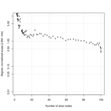
(a) n100w750

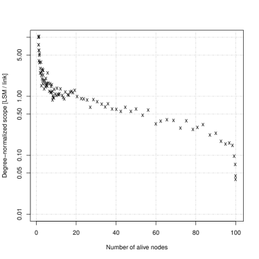
(b) n100w250

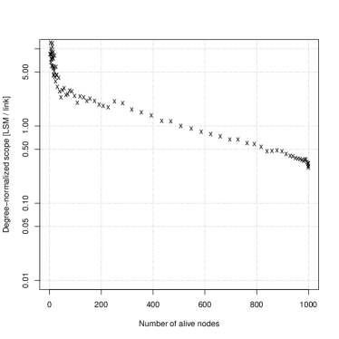
(c) n1000w2000

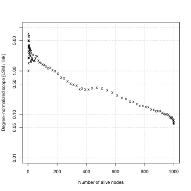
(d) n1000w1000

Figure 33: Comparison of logarithmic degree-normalized scope and number of alive nodes for RQ2

The four plots in Figure 34 show the i-kTC-to-b-kTC link state modification ratio vs. the number of alive nodes. As in Figure 33, each data point represents the results of a TC run at a particular point in time during the simulation, averaged across all 15 simulation runs per configuration. Please note that also here the y-axis is logarithmic due to the large range of the data.

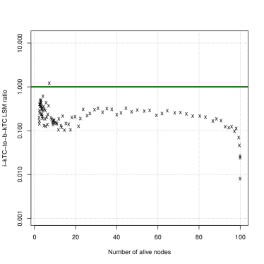
(a) n100w750

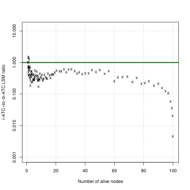
(b) n100w250

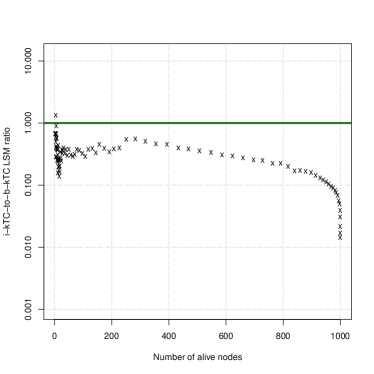
(c) n1000w2000

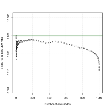
(d) n1000w1000

Figure 34: Comparison of logarithmic i-kTC-to-b-kTC link state modification ratio and number of alive nodes for RQ2

Discussion

The plots in Figure 33 allow us to investigate in how far the number of alive nodes and the node degree correlate with the degree-normalized scope of a TC run. In all plots, the degree-normalized scope tends to decrease with increasing number of alive nodes. This is a very positive result because it shows that the scope, when normalized by the node out-degree, is even positively affected by the size of the topology.

Finally, we discuss the benefit of applying i-kTC in comparison to b-kTC using Figure 34. Pleasantly, for all configurations, the fraction of link state modifications required for performing i-kTC in comparison to b-kTC decreases significantly. In all four configurations, i-kTC outperformed b-kTC in between $89\text{\,}\mathrm{\char 37\relax}$ and $99\text{\,}\mathrm{\char 37\relax}$ of all TC runs per configuration, i.e., between 106 (for n1000w1500) and 118 (for n1000w2000) out of 119 TC runs. To sum up, we may answer RQ2 as follows.

• i-kTC is theoretically unbounded and, therefore, not strictly incremental. Still, from a practical point of view, we showed that the cost in terms of link state modifications is bounded and mainly determined by the average node out-degree, which is a local property. Thus, i-kTC behaves incrementally in the considered scenarios.

• i-kTC was able to clearly outperform b-kTC in our simulation study. The benefit of invoking i-kTC even increases with increasing number of alive nodes, i.e., with increasing topology size.

6.5 RQ3–Performance

Metrics

To assess the performance of the integration of eMoflon and the Simonstrator, we measure and compare the CPU time of executing the GT-based implementation (i.e., the context event handling, the TC algorithm, the consistency checks) and the remaining simulation.

Results

Table 10 provides an overview of the execution time measurements for each configuration, averaged over all 15 runs per configuration. We list (i) the time for the algorithmic part (GT algo), i.e., handling context events and invoking TC, (ii) the time required for invoking the (optional) consistency checks (GT checks), which were active during the whole simulation study to increase the confidence in the correctness of our implementation (see Section 6.3), and (iii) the time for performing the remainder of the simulation (Sim.). The configurations are sorted increasinly by size and density of the initial topology.

Table 10: Quantitative comparison of execution time for RQ3. n+m: Topology size.

ID	n+m	GT Algo [min]	GT Checks [min]	Sim. [min]	Total [min]	GT Algo / Total [%]
n100w750	912	0.01	0.00	0.76	0.77	0.9
n100w500	1 751	0.02	0.01	0.76	0.79	2.7
n100w250	5 261	0.69	0.19	0.93	1.81	38.2
n1000w2000	13 683	0.13	0.08	96.98	97.18	0.1
n1000w1500	23 092	0.56	0.33	125.12	126.00	0.4
n1000w1000	49 072	7.46	2.83	170.52	180.81	4.1

Discussion

The numbers in Table 10 are impressive: For three out of six configurations, the overhead of invoking the GT-based implementation is below $1\text{\,}\mathrm{\char 37\relax}$ (n100w750, n1000w2000, n100w500). In further two out of six configurations, the overhead is below $5\text{\,}\mathrm{\char 37\relax}$ (n100w500, n1000w1000). Only in the densest configuration n100w250 with an initial average out-degree of approx. 50, the overhead is remarkably high ($38\text{\,}\mathrm{\char 37\relax}$), which is acceptable because a configuration of such density reflects a border case. When comparing the execution time of the algorithm and the consistency checking part of the GT implementation, we recognize that between approx. $25\text{\,}\mathrm{\char 37\relax}$ and $33\text{\,}\mathrm{\char 37\relax}$ of the execution time of the GT implementation is used for checking consistency. For this reason, it may be reasonable to disable consistency checking as soon as the developer has gained sufficient confidence in her implementation of the GT algorithm to gain even more performance. Still, we experienced that checking consistency continuously during the simulation is a valuable feature because it aids in identifying even subtle bugs due to the huge number of checked topologies. The fact that the execution time of the GT algorithm for the largest configuration (i.e., n1000w1000) makes up only $4\text{\,}\mathrm{\char 37\relax}$ of the total execution time shows that our implementation allows simulations even of large topologies and that it is definitely not the bottleneck for such large scenarios. To sum up, we may answer RQ3 as follows.

• The fraction of CPU time that is requird for performing TC and context event greatly varies depending on the configuration. For five out of six configurations, the fraction is below $5\text{\,}\mathrm{\char 37\relax}$.

• The execution time of i-kTC is definitely reasonable for the considered topologies.

6.6 RQ4–Generalizability

In the following, we qualitatively discuss the general applicability of the proposed approach.

6.6.1 Is meta-modeling suitable to specify all relevant properties of WSN topologies?

Based on our experience, we claim that meta-modeling does not impose any restrictions on the complexity of the specified topologies. Meta-modeling concepts that are available in both theory and practice are, e.g., arbitrary attributes of nodes, links, and whole topologies (single-, set-, or list-valued, potentially using custom datatypes) as well as (multiple) inheritance. More advanced algorithms that also take overlay constraints into account [68, 73, 53] would require to model paths and constraints on paths, which is also easily possible using meta-modeling.

6.6.2 Are GT rules suitable to specify context events and TC operations?

We believe that GT is suitable to model context events and TC operations in general because graph-based models and GT rules are natural means to represent the structure and modification of topologies.

6.6.3 Are graph constraints and the proposed constructive approach suitable to specify and ensure the preservation of consistency constraints and optimization goals of typical TC algorithms?

Graph constraints as first introduced in [42] and adopted in this paper are suitable to specify required (in case of positive graph constraints) and forbidden (in case of negative graph constraints) substructures in topologies of finite size but, thanks to [43], with arbitrary complex attribute constraints. Still, our running example, kTC, reveals that certain consistency constraints and optimization goals cannot be expressed using this type of graph constraints: Physical, weak and strong connectivity are not expressible because of the required constraints over paths of links of arbitrary length. Additional typical constraints are, e.g., that the output topology should be $k$-connected, a directed acyclic graph (DAG) or even a tree/forest. In [74, 75], Habel and Radke present $HR^{*}$ constraints, a new type of graph constraints that allow to express path-related properties. Fortunately, the constructive approach is applicable to $HR^{*}$ constraints in principle; in future work, we will investigate the applicability of $HR^{*}$ constraints to specify, e.g., connectivity of topologies. An additional feature of meta-models that was not required in this case study is type inheritance. In [76], the authors describe how the constructive approach may be applied to meta-models with edge and node type inheritance. The propose to flatten the original meta-model into an equivalent meta-model without type inheritance based on which the original constructive approach of [42, 43] may be applied.

From our experience, we may say that at least the optimization goals of a large class of TC algorithms may be specified using graph constraints. These TC algorithms operate on local knowledge, e.g., only of neighbors that are at most two hops away, so-called local algorithms [77]. This restriction is necessary because sensor nodes tend to have limited working memory (to store the local topology) and because acquiring the neighborhood topology of a node is the more expensive in terms of bandwidth and execution the larger the required topology becomes [53]. Therefore, we may answer the question as follows: Graph constraints are suitable to specify the optimization goals of a huge class of TC algorithms, while crucial consistency constraints currently need to be proved manually. In total, this is still a considerable advantage over the current state of the art, which only allows to verify or test that a TC algorithm fulfills the desired consistency constraints and optimization goals a posteriori.

6.6.4 Is a TC developer able to apply the described methodology?

If we want to establish a new development methodology for TC algorithms, it is crucial that the target audience, i.e., the developers of TC algorithms, is capable of applying it.

The first step of our methodology is to capture the relevant properties (i.e., classes with their attributes and associations) of the topologies that shall be processed by the TC algorithm (see Section 2). To successfully perform this step, a developer needs to have a working background in meta-modeling, which is realistic as several industrial success stories prove [78].

The second step of our methodology is the specification of optimization goals and consistency constraints in terms of graph constraints (see Section 3). While this is certainly a non-trivial task, the adoption of a constraint specification languages (e.g., the Object Constraint Language [79]) in practice indicates that this step should also be feasible for a developer. In Section 3.5, the constraint-based formulation of kTC was used to prove that the output topology is connected whenever the input topology fulfills weak consistency. A developer may need to prove this and similar properties at this step for other TC algorithms. However, when analyzing the TC literature, we recognize that developers of TC algorithms already perform this step today: They prove properties such as planarity or connectivity of the topology, boundedness of node degree or termination based on their formal representation of the proposed TC algorithm (e.g., in [6, 12]). For this reason, we believe that it is reasonable for a TC developer to succeed in proving properties using a graph constraint-based specification of the TC algorithm.

The third step of our methodology is to describe relevant context events and TC operations using GT rules (see Section 4). As described in [78], it is also a realistic assumption that developers acquire these skills. Additionally, the GT rules presented in Section 4 will be reusable, maybe with modifications, in a large number of cases. For instance, the node removal rule $R_{\textrm{-n}}$ and the link removal rule $R_{\textrm{-e}}$ may probably be re-used out-of-the-box, while the node addition rule $R_{\textrm{+n}}$, the link addition rule $R_{\textrm{+e}}$, and the weight modification rule $R_{\textrm{mod-w}}$ may have to be updated to reflect the particular node and link attributes of the considered class of topologies. These considerations are backed by observations in the literature that TC algorithms (not only in the WSN domain) are typically composed of elementary topology modification operations (e.g., link removal) [50].

The fourth step of our methodology is the refinement of the specified GT rules to preserve the specified graph constraints (see Section 5.1). While the concrete applications of the refinement algorithm as described in Sections 5.1.3, 5.1.4, 5.1.5 and 5.1.5 were carried out manually for this paper, the rule refinement algorithm may in principle be automated. As discussed in Section 6.3, performing this step manually is error-prone and tedious. Therefore, a powerful tool support is required to aid the developer in analyzing and filtering the resulting application conditions to come up with a set of rules that is readable and efficient to evaluate.

The fifth step of our methodology is the derivation of restoration operations for unrestrictable GT rules that were refined with additional application conditions during the refinement step (see Section 5.2). In this paper, we do not provide a precise algorithm for automatically deriving restoration operations from a given application condition. Yet, such an algorithm may exist at least for graph constraints as used in our approach. In this case, tool support for automating should be developed as for the refinement step.

The sixth step of our methodology is the simulation-based evaluation of the specified TC algorithm. The existing tool support, consisting of a model-based adapter between eMoflon and the Simonstrator, may be re-used if the Simonstrator is deemed appropriate by the developer to carry out the evaluation. The only required modification is an update of the synchronization objects in the Simonstrator and the topology model. If a different network simulator or a different GT tool is to be used to carry out the evaluation, more development effort is required. Still, the existing tool support may serve as a template for implementing the desired adapter between the GT tool and the network simulator of the developer’s choice.

In summary, the meta-modeling part, the specification of GT rules and graph constraints, and the adaptation of the integration between the GT tool and the simulator can realistically be carried out by a developer of TC algorithms. The refinement algorithm and the derivation of restoration operations, which form the core parts of our methodology, still require advanced tooling to support the TC developer.

6.7 Discussion of Threats to Validity and Summary of Evaluation

We considered threats to external validity [80], i.e., the general applicability of our approach, as the major threat to validity. While this paper discussed the construction of one particular TC algorithm in detail due to space limitations, we mitigated this threat by dedicating RQ4 to it (Section 6.6). The performance evaluation in Section 6.5 mitigates this threat from a practical point of view: Our proof-of-concept implementation of the integration of eMoflon and the Simonstrator is applicable to WSN topologies of realistic size and does not impose an unreasonable overhead.

We considered threats to internal validity, i.e., the soundness of the presented results, when discussing RQ1–Correctness. We analyzed in detail the possible sources of specification and implementation problems (e.g., the manual creation of restoration operations) and applied measures to minimize or mitigate them (e.g., by continuously checking consistency during the numerous iterations in the simulation study). In Table 11, we concisely summarize the results of this evaluation.

Table 11: Summary of answers to the research questions

RQ	Sec.	Result
RQ1–Correctness	6.3	We carefully analyzed potential sources of errors during the steps of the methodology and described the applied mitigation strategies. All of the 21 600 consistency checks during the simulation study were successful, which fosters the confidence in the correctness of our implementation.
RQ2–Incrementality	6.4	The execution of context event handlers is unbounded and, therefore, the developed algorithm is theoretically not strictly incremental. However, the simulation showed that the scope of context events is limited by a constant that is independent of the number of alive nodes.
RQ3–Performance	6.5	In the smallest and densest configuration, n100w250, GT consumed $38\text{\,}\mathrm{\char 37\relax}$ of the execution time. In all other five of six configurations, GT consumed less than $5\text{\,}\mathrm{\char 37\relax}$ of the execution time.
RQ4–Generalizability	6.6	Meta-modeling and GT rules are suitable to specify arbitrary WSN topologies and their modifications by context events and TC algorithms. Typical optimization goals of the large class of local TC algorithms can naturally be modeled using graph constraints; certain consistency constraints such as connectivity may not be expressed using graph constraints. A developer of TC algorithms should be capable of applying our methodology in practice if the existing tooling is extended appropriately.

7 Related Work

In this section, we survey related work from the fields of modeling and checking consistency properties and formal methods as well as model-based software engineering in the communication network engineering domain.

Specifying, checking and enforcing consistency properties

Model checking [81] is an analysis technique used to verify particular properties of a system a posteriori, i.e., after a specification of the desired properties and an implementation of the regarded system has been constructed. If an abstract symbolic problem specification [82] is missing, model checking tools are often limited to a finite model size. The approach in this paper constructively integrates constraints a priori at design time into an already executable formal specification of a TC algorithm rather than checking whether specified properties are fulfilled a posteriori (either at design time or at runtime). This correct-by-construction approach (e.g., [83, 84, 85]) has the positive side-effect that we can prove that topologies of any size are consistent without any needs to find a finite abstraction of the infinite set of all possible topologies.

In [42], graphical consistency constraints, which express the fact that particular combinations of nodes and edges should be present in or absent from a graph, are translated into application conditions of GT rules. This technique has been generalized to the framework of HLR categories [22] and extended to cope with attributes [43]. The basic idea is to translate consistency conditions, characterizing consistent graphs, into post-conditions of GT rules, which may then be transformed into application conditions of the rules. This paper applies and extends this generic methodology for the practical and complex application scenario of developing TC algorithms. Our extension consists of an additional, domain-specific step that translates some of the derived application conditions into pre- and post-processing rules that ensure that the corresponding application conditions are always fulfilled and may, thus, be removed from the rule. These new domain-specific relaxation and re-enforcement techniques for constraints and application conditions are needed to bypass a critical—and from a practical point of view often unrealistic assumption—made in [42]: A GT-rule with additional application conditions preserves some graph constraints if the application conditions may block any harmful execution of this rule, and if the processed graph never contains any constraint violations. Both assumptions are violated in our scenario, where context events may add, modify, and remove topology elements without any restrictions.

Consistency properties may be expressed using a variety of formal frameworks. In this paper, we use graphical consistency constraints [42], which are suitable to specify properties based on a fixed number of graph elements, e.g., the triangle of links in kTC. However, certain consistency properties, such as connectivity, may not be expressed in this framework. For such properties, more expressive formal frameworks such as (counting) second-order monadic logic [42, 86] or nested graph constraints [41, 58] exist. In this paper, connectivity of topologies is the only consistency property that cannot be expressed using graphical consistency constraints; therefore, we manually proved that this property is fulfilled.

In [87], model transformations are categorized based on the way that their application affects the consistency of a model. In their categorization, a transformation may basically either preserve or establish consistency. Consistency is preserved by a transformation if models that were consistent before the transformation are consistent afterwards as well. Consistency is established by a transformation if models that might not be consistent before the transformation are consistent afterwards. In this paper, preservation of weak consistency is achieved because we assume that the initial network topology is weakly consistent and because the refined TC and context event rules preserve the TC graph constraints that imply weak consistency.

A prominent alternative language for specifying constraints is the Object Constraint Language (OCL) [88] and its visual extension VisualOCL [89]. Current research focuses on translating OCL constraints into graph constraints [90, 91]. In Story Decision Diagrams [92], a complex (graph) constraint is formalized using a directed acyclic graph data structure that resembles Story Diagrams, which have been employed in this paper to define the control flow of TC operations. While the graph constraints considered in this paper could easily be expressed using Story Decisions Diagrams, to the best of our knowledge, no work exists that allows to transform postconditions formulated as Story Decision Diagram into preconditions of GT rules.

Formal methods in communication network engineering

The need for supporting or even driving the development of novel network communication protocols using formal methods has been recognized already in the 1980s [93], and even today, formal methods are continuously gaining importance in the networking engineering community [16].

Formal analysis of consistency properties of network protocols has already revealed special cases in which the implemented algorithms violate crucial (topological) constraints [14, 15, 94, 95]. In [14], the SPIN model checker [96] is used to analyze the Session Initiation Protocol (SIP) for specification flaws. In [15], the lightweight modeling language Alloy [97] is used to find specification flaws in the famous peer-to-peer protocol Chord [98]. In [95], statistical model checking is applied to analyze AODV and DYMO, two famous routing protocols for wireless mesh networks. In [99], model checking is applied to detect bugs and to point at their causes in the TC algorithm LMST, leading to an improved implementation thereof. In contrast to the aforementioned contributions, this paper focuses on preserving consistency properties in a constructive way rather than analyzing existing protocols a posteriori.

In [11], a three-stage development process of WSN algorithms—consisting of formalization, simulation evaluation, and testbed evaluation—is emphasized as an important means of verifying WSN algorithms. While the authors focus on the role of testbed simulations (compared to simulation), the focus of this paper is to reduce the gap between the formalization and the simulation part.

In [100], Nareyek highlights that avoiding consistency checks at runtime by constructively integrating constraints into the preconditions of rules of decision agents may also increase the performance.

Visual languages and models in the context of telecommunications

Visual and model-based languages techniques have shown to be suitable to describe [101] and to construct [19] optimization algorithms for communication networks. Message sequence charts [102], for instance, have already been used to document protocol standards of communication systems; the same is true for object-oriented modeling languages like ROOM [103], which was one of the first (truly) object-oriented modeling tools successfully used by the telecommunication industry. Some examples of distributed system visual programming languages are G-Net [34, 35], Prograph [104], DVispatch [105], which rely on different programming paradigms and formalisms (such as Petri-Nets [106] and Flow-Graphs [107]). In [68], an approach for the GT-based rapid prototyping of variants of TC algorithms is proposed. In a case study, the GT tool eMoflon [23] is used to derive two batch variants—l-kTC and g-kTC—of the TC algorithm kTC [6, 71], which filter the selected links of the marking step of TC based on additional, application-specific constraints. In [73], the batch algorithms l-kTC and g-kTC are evaluated in detail in a simulation study using the Simonstrator platform [61]. In this paper, we use the same tooling as in [68, 73] for the simulation study, but we focus on deriving incremental TC algorithms that are correct by construction rather than introducing complex additional consistency constraints.

In the following, we list further approaches to the graph-based and model-based construction of TC algorithms. In [108], an extension to Agilla [44], a model-driven middleware for developing WSN applications, is proposed that introduces an instruction set for reading the current remaining energy of sensor nodes. In [45], a model-driven development process is proposed that allows to design TC algorithms based on meta-models and state charts and then to generate platform-specific code from this representation. The focus of their approach lies on a complete tool chain from a platform-independent model to the platform-specific, compilable code; correctness properties of the developed algorithms have to be ensured manually. In [32], a model-driven tool for developing WSN applications called Matilda is presented. Based on a custom UML profile [29] for sensor networks, the authors describe the domain structure using class diagrams, concrete network instances using instance diagrams, and the behavior of the sensor nodes using sequence diagrams. The authors propose to extend their development process with techniques for checking correctness. In [46], a model-based approach for developing WSN algorithms in a stepwise manner is proposed, which separates the concerns of designing the WSN application logic from the handling of network-related concerns. The focus of their approach is on decomposing the development process of WSN applications. In [47], the modeling and simulation framework VisualSense is presented, which operates on top of the modeling framework for heterogeneous devices Ptolemy II [109]. The platform provides a visual modeling language for specifying the data flow while at the same time abstracting from the concrete topology of the WSN. In [110], the model-based development environment ScatterClipse is presented, which has been developed to provide an integrated development workflow for sensor applications that run on the ScatterWeb [111] WSN platform. ScatterClipse adopts the Model-Driven Software Development workflow of the OMG [112] and allows the user to specify rules that validate the syntactic and semantic correctness of the developed models. However, no means for specifying consistency constraints of the network topology exists. In [113], the virtual-machine environment Maté is presented, which provides a high-level application programming interface for WSN algorithms as well as distribution and replication mechanisms that allow for an efficient deployment of WSN algorithms into a hardware testbed. The focus of [113] lies on the efficient testing of WSN algorithms in a virtual environment. This list of approaches for the model-driven development of TC algorithms shows that most frameworks are centered around (i) providing a thorough development process or (ii) separating the concerns of the domain engineer from those of the networking engineer In contrast to this paper, none of these approaches considers the provable correctness of the developed algorithms as a core concern.

In [33], MechatronicUML is presented as a comprehensive framework for specifying and formally analyzing mechatronic systems. The structure of systems is described by means of component diagrams similar to UML, the behavior of systems is described by means of state charts, and architectural reconfigurations are described by means of GT rules using the Fujaba real-time tool suite [114], which is a branch of the Fujaba GT tool [28]. Based on these formal foundations, the authors use the verification techniques model checking [24] and proof by induction [115] to verify safety properties of the modeled systems. While the approach proposed in [33] presents a mature and powerful environment for developing and verifying mechatronic systems, safety properties are, again, checked a posteriori, whereas in our approach, safety properties are integrated into the development process.

A series of publications by Scheideler and others use graph theory for constructing provably correct and efficient algorithms for adapting topologies of WSNs and other applications such as distributed search overlays (see, for instance, [77, 19, 116, 117, 118]). While their approach ensures that consistency properties and optimization goals are fulfilled by the derived algorithm, the structured transformation into an executable implementation is not so obvious. In this paper, in contrast, we formalize the possible modifications of the network topology as GT rules and we formalize the consistency properties and optimization goals as graph constraints. On the one hand, this allows to prove the correctness of the refined GT rules in terms of the specified graph constraints. On the other hand, the derived GT rules can be directly used to implement and evaluate the TC algorithm.

8 Conclusion

This section concludes the paper and highlights possible directions of future research.

8.1 Summary

In this paper, we describe a model-based methodology for developing TC algorithms, which select a subset of the links of a communication network that fulfills specified consistency properties and optimization goals. We use GT rules to describe possible TC operations, which are applied by a TC algorithm to mark selected links, as well as context events, which specify modifications of the topology by the environment. We specify consistency and optimization properties of output topologies of TC algorithms using graph constraints, which are then used to refine the TC and context event rules in a way that applying the rules preserves the graph constraints. We apply the constructive approach to the TC algorithm kTC. The discussion of a simulation-based evaluation shows that the constructed TC algorithms may be directly evaluated in a number of realistic simulation scenarios. We showed that (i) the implementation passed all 21 600 consistency checks, (ii) the derived algorithm operates incrementally in practice, (iii) the performance of the developed integration between the GT tool eMoflon and the network simulation platform Simonstrator is very satisfactory, and (iv) the proposed methodology is applicable to a large class of TC algorithms.

8.2 Outlook

The results of this paper open up various possible lines of research. A first line of research addresses the partial automation of our constructive methodology: The refinement procedure described and applied in Section 5 is formally founded and the resulting rules are “correct by construction”. Still, performing the refinement procedure manually is error-prone and should be automated as far as possible. We showed that the number of additional application conditions may be reduced considerably if we assume that particular constraints (e.g., the structural constraints) hold prior to each execution of a TC rule. It remains to investigate if it is possible to automatically derive repair operations from a set of application conditions.

A second line of research addresses the simulation study. Simulating a distributed execution of GT based on a to-be-designed GT protocol is desirable to be able to investigate concurrency and timing issues already inside the simulator.

The specification of the TC algorithm in this paper is suitable to operate not only in a centralized way on the whole topology, but also in a distributed way on the local view of each node, which typically consists of all nodes that are two or three hops away from the node. Finally, we have to overcome the limitation that the TC algorithm is executed offline, i.e., outside the running simulation, which is currently halted during the execution of the TC algorithm. A truly distributed, asynchronous implementation will open up challenging research questions, e.g., about conflicting rule applications and asynchronicity.

A third line of research addresses the evaluation of the developed TC algorithms in a hardware testbed. This step is especially challenging because wireless nodes are usually programmed in C/C++ and typically have strictly limited resources in terms of code size and memory. The GT tool eMoflon, which we applied for the simulation study, is currently only able to generate Java code. We are currently performing first experiments in generating C code for the WSN platform Contiki [119].

References

References

- Santi [2005] P. Santi, Topology Control in Wireless Ad Hoc and Sensor Networks, ACM computing surveys (CSUR) 37 (2) (2005) 164–194, URL http://dx.doi.org/10.1145/1089733.1089736.
- Yick et al. [2008a] J. Yick, B. Mukherjee, D. Ghosal, Wireless Sensor Network Survey, Computer Networks 52 (12) (2008a) 2292–2330, URL http://dx.doi.org/10.1016/j.comnet.2008.04.002.
- Wang [2008] Y. Wang, Topology Control for Wireless Sensor Networks, in: Wireless Sensor Networks and Applications, Springer, 113–147, URL http://dx.doi.org/10.1007/978-0-387-49592-7_5, 2008.
- Sun et al. [2011] R. Sun, J. Yuan, I. You, X. Shan, Y. Ren, Energy-aware weighted graph based dynamic topology control algorithm, Simulation Modelling Practice and Theory 19 (8) (2011) 1773 – 1781, ISSN 1569-190X, URL http://dx.doi.org/10.1016/j.simpat.2010.09.002.
- Li et al. [2013] M. Li, Z. Li, A. V. Vasilakos, A Survey on Topology Control in Wireless Sensor Networks: Taxonomy, Comparative Study, and Open Issues, Proceedings of the IEEE 101 (12) (2013) 2538–2557, ISSN 0018-9219, URL http://dx.doi.org/10.1109/JPROC.2013.2257631.
- Schweizer et al. [2012] I. Schweizer, M. Wagner, D. Bradler, M. Mühlhauser, T. Strufe, kTC - Robust and Adaptive Wireless Ad-Hoc Topology Control, in: Proc. of the Intl. Conf. on Computer Communications and Networks, 1–9, URL http://dx.doi.org/10.1109/ICCCN.2012.6289318, 2012.
- Wattenhofer and Zollinger [2004a] R. Wattenhofer, A. Zollinger, XTC: A Practical Topology Control Algorithm for Ad-Hoc Networks, in: Proc. of Parallel and Distributed Processing Symposium, 2004., 216–223, URL http://dx.doi.org/10.1109/IPDPS.2004.1303248, 2004a.
- Li et al. [2005] N. Li, J. Hou, L. Sha, Design and analysis of an MST-based topology control algorithm, IEEE Trans. on Wireless Communications 4 (3) (2005) 1195–1206, URL http://dx.doi.org/10.1109/TWC.2005.846971.
- Machado and Tekinay [2008] R. Machado, S. Tekinay, A Survey of Game-Theoretic Approaches in Wireless Sensor Networks, Computer Networks 52 (16) (2008) 3047–3061, URL http://dx.doi.org/10.1016/j.gaceta.2008.07.003.
- Shi et al. [2012] H.-Y. Shi, W.-L. Wang, N.-M. Kwok, S.-Y. Chen, Game Theory for Wireless Sensor Networks: A Survey, Sensors 12 (7) (2012) 9055–9097, URL http://dx.doi.org/10.3390/s120709055.
- Papadopoulos et al. [2016] G. Z. Papadopoulos, K. Kritsis, A. Gallais, P. Chatzimisios, T. Noel, Performance evaluation methods in ad hoc and wireless sensor networks: a literature study, IEEE Communications Magazine 54 (1) (2016) 122–128, ISSN 0163-6804, URL http://dx.doi.org/10.1109/MCOM.2016.7378437.
- Chu and Sethu [2012] X. Chu, H. Sethu, Cooperative Topology Control with Adaptation for Improved Lifetime in Wireless Ad-Hoc Networks, in: Proc. of INFOCOM 2012, 262–270, URL http://dx.doi.org/10.1109/INFCOM.2012.6195667, 2012.
- Monderer and Shapley [1996] D. Monderer, L. S. Shapley, Potential Games, Games and Economic Behavior 14 (1) (1996) 124 – 143, ISSN 0899-8256, URL http://dx.doi.org/10.1006/game.1996.0044.
- Zave [2008] P. Zave, Understanding SIP through Model-Checking, in: Principles, Systems and Applications of IP Telecommunications. Services and Security for Next Generation Networks, vol. 5310, Springer, 256–279, URL http://dx.doi.org/10.1007/978-3-540-89054-6_13, 2008.
- Zave [2012] P. Zave, Using Lightweight Modeling to Understand Chord, SIGCOMM Comput. Commun. Rev. 42 (2) (2012) 49–57, URL http://dx.doi.org/10.1145/2185376.2185383.
- Qadir and Hasan [2015] J. Qadir, O. Hasan, Applying Formal Methods to Networking: Theory, Techniques, and Applications, Communications Surveys Tutorials, IEEE 17 (1) (2015) 256–291, ISSN 1553-877X, URL http://dx.doi.org/10.1109/COMST.2014.2345792.
- Völter et al. [2013] M. Völter, T. Stahl, J. Bettin, A. Haase, S. Helsen, Model-Driven Software Development: Technology, Engineering, Management, John Wiley & Sons, ISBN 9781118725764, 2013.
- Blendin et al. [2015] J. Blendin, J. Rückert, T. Volk, D. Hausheer, Adaptive Software Defined Multicast, in: Proc. of Network Softwarization (NetSoft 2015), 1–9, URL http://dx.doi.org/10.1109/NETSOFT.2015.7116158, 2015.
- Jacob et al. [2009] R. Jacob, A. Richa, C. Scheideler, S. Schmid, H. Täubig, A Distributed Polylogarithmic Time Algorithm for Self-stabilizing Skip Graphs, in: Proc. of the ACM Symposium on Principles of Distributed Computing, ACM, 131–140, URL http://dx.doi.org/10.1145/1582716.1582741, 2009.
- Kniesburges et al. [2014] S. Kniesburges, A. Koutsopoulos, C. Scheideler, Re-Chord: A Self-stabilizing Chord Overlay Network, Theory of Computing Systems 55 (3) (2014) 591–612, URL http://dx.doi.org/10.1007/s00224-012-9431-2.
- Rozenberg [1997] G. Rozenberg (Ed.), Handbook of Graph Grammars and Computing by Graph Transformation, vol. 1: Foundations, World Scientific, URL http://dx.doi.org/10.1142/3303, 1997.
- Ehrig et al. [2006] H. Ehrig, K. Ehrig, U. Prange, G. Taentzer, Fundamentals of Algebraic Graph Transformation, Springer, URL http://dx.doi.org/10.1007/3-540-31188-2, 2006.
- Leblebici et al. [2014] E. Leblebici, A. Anjorin, A. Schürr, Developing eMoflon with eMoflon, in: Proc. of ICMT 2014, 138–145, URL http://dx.doi.org/10.1007/978-3-319-08789-4_10, 2014.
- Rensink [2004] A. Rensink, The GROOVE Simulator: A Tool for State Space Generation, in: Applications of Graph Transformations with Industrial Relevance, vol. 3062, Springer, 479–485, URL http://dx.doi.org/10.1007/978-3-540-25959-6_40, 2004.
- Arendt et al. [2010] T. Arendt, E. Biermann, S. Jurack, C. Krause, G. Taentzer, Henshin: Advanced Concepts and Tools for In-Place EMF Model Transformations, in: Model Driven Engineering Languages and Systems, vol. 6394, Springer, 121–135, URL http://dx.doi.org/10.1007/978-3-642-16145-2_9, 2010.
- Geiß et al. [2006] R. Geiß, V. Batz, D. Grund, S. Hack, A. M. Szalkowski, GrGen: A Fast SPO-Based Graph Rewriting Tool, in: Proc. Intl. Conference on Graph Transformation, vol. 4178, Springer, 383–397, URL http://dx.doi.org/10.1007/11841883_27, 2006.
- Taentzer [2000] G. Taentzer, AGG: A Tool Environment for Algebraic Graph Transformation, in: Proc. of AGTIVE’99, vol. 1779, Springer, 481–490, URL http://10.1007/3-540-45104-8_41, 2000.
- Nickel et al. [2000] U. Nickel, J. Niere, A. Zündorf, The FUJABA Environment, in: Proc. of ICSE, ACM, 742–745, URL http://dx.doi.org/10.1145/337180.337620, 2000.
- Group [2005] O. M. Group, UML Specification, Version 2.0, OMG, URL http://www.omg.org/spec/UML/, 2005.
- Gomaa [2001] H. Gomaa, Designing Concurrent, Distributed, and Real-time Applications with UML, in: Proc. of the 23rd Intl. Conference on Software Engineering, IEEE, 737–738, URL http://dl.acm.org/citation.cfm?id=381473.381619, 2001.
- de Wet and Kritzinger [2005] N. de Wet, P. Kritzinger, Using UML models for the performance analysis of network systems, Computer Networks 49 (5) (2005) 627 – 642, ISSN 1389-1286, URL http://dx.doi.org/10.1016/j.comnet.2005.05.007.
- Wada et al. [2007] H. Wada, P. Boonma, J. Suzuki, K. Oba, Modeling and Executing Adaptive Sensor Network Applications with the Matilda UML Virtual Machine, in: Proc. of the IASTED ICSE and Applications, ACTA Press, ISBN 978-0-88986-706-2, 216–225, 2007.
- Schäfer and Wehrheim [2010] W. Schäfer, H. Wehrheim, Model-Driven Development with Mechatronic UML, in: Graph Transformations and Model-Driven Engineering, vol. 5765, Springer, 533–554, URL http://dx.doi.org/10.1007/978-3-642-17322-6_23, 2010.
- Chen et al. [1993] T.-C. Chen, Y. Deng, S.-K. Chang, A Simulator for Distributed Systems using G-Nets, Modeling and Simulation 23 (1993) 2705–2705.
- Ng et al. [1996] K. Ng, J. Kramer, J. Magee, N. Dulay, A Visual Approach to Distributed Programming, in: Tools and Environments for Parallel and Distributed Systems, vol. 2, Springer, 7–31, URL http://dx.doi.org/10.1007/978-1-4615-4123-3_2, 1996.
- Zhang [2007] K. Zhang, Visual Languages and Applications, Springer, URL http://dx.doi.org/10.1007/978-0-387-68257-0, 2007.
- Marriott and Meyer [1998] K. Marriott, B. Meyer, Visual Language Theory, Springer, URL http://dx.doi.org/10.1007/978-1-4612-1676-6, 1998.
- Chang et al. [1990] S.-K. K. Chang, E. Glinert, J. G. Bonar, M. Graf, A. T. Berztiss, Principles of Visual Programming Systems, Prentice Hall Professional Technical Reference, ISBN 013710765X, 1990.
- Bauer et al. [1989] F. Bauer, B. Moller, H. Partsch, P. Pepper, Formal Program Construction by Transformations-Computer-Aided, Intuition-Guided programming, IEEE Trans. on Software Engineering 15 (2) (1989) 165–180, URL http://dx.doi.org/10.1109/32.21743.
- France and Rumpe [2007] R. France, B. Rumpe, Model-driven Development of Complex Software: A Research Roadmap, in: Future of Software Engineering, IEEE, ISBN 0-7695-2829-5, 37–54, URL http://dx.doi.org/10.1109/FOSE.2007.14, 2007.
- Habel and Pennemann [2005] A. Habel, K.-H. Pennemann, Nested Constraints and Application Conditions for High-Level Structures, in: Formal Methods in Software and Systems Modeling, vol. 3393, Springer, ISBN 978-3-540-24936-8, 293–308, URL http://dx.doi.org/10.1007/978-3-540-31847-7_17, 2005.
- Heckel and Wagner [1995] R. Heckel, A. Wagner, Ensuring Consistency of Conditional Graph Rewriting – A Constructive Approach, in: Proc. of Joint COMPUGRAPH/SEMAGRAPH Workshop, vol. 2, Elsevier, 118–126, URL http://dx.doi.org/10.1016/S1571-0661(05)80188-4, 1995.
- Deckwerth and Varró [2014] F. Deckwerth, G. Varró, Generating Preconditions from Graph Constraints by Higher Order Graph Transformation, ECEASST 67 (2014) 1–14, URL http://dx.doi.org/10.14279/tuj.eceasst.67.945.
- Fok et al. [2009] C.-L. Fok, G.-C. Roman, C. Lu, Agilla: A Mobile Agent Middleware for Self-adaptive Wireless Sensor Networks, ACM Trans. of Autonomous Adaptive Systems 4 (3) (2009) 16:1–16:26, URL http://dx.doi.org/10.1145/1552297.1552299.
- Rodrigues et al. [2015] T. Rodrigues, F. Delicato, T. Batista, P. Pires, L. Pirmez, An approach based on the domain perspective to develop WSAN applications, Software & Systems Modeling (2015) 1–29URL http://dx.doi.org/10.1007/s10270-015-0498-5.
- Tei et al. [2015] K. Tei, R. Shimizu, Y. Fukazawa, S. Honiden, Model-Driven-Development-Based Stepwise Software Development Process for Wireless Sensor Networks, IEEE Trans. on Systems, Man, and Cybernetics 45 (4) (2015) 675–687, URL http://dx.doi.org/10.1109/TSMC.2014.2360506.
- Baldwin et al. [2004] P. Baldwin, S. Kohli, E. A. Lee, X. Liu, Y. Zhao, Modeling of Sensor Nets in Ptolemy II, in: Proc. of the Intl. Symposium on Information Processing in Sensor Networks, ACM, 359–368, URL http://dx.doi.org/10.1145/984622.984675, 2004.
- Kluge et al. [2015] R. Kluge, G. Varró, A. Schürr, A Methodology for Designing Dynamic Topology Control Algorithms via Graph Transformation, in: Theory and Practice of Model Transformations, vol. 9152, Springer Intl. Publishing, ISBN 978-3-319-21154-1, 199–213, URL http://dx.doi.org/10.1007/978-3-319-21155-8_15, 2015.
- Karp and Kung [2000] B. Karp, H. T. Kung, GPSR: Greedy Perimeter Stateless Routing for Wireless Networks, in: Proceedings of the 6th Annual Intl. Conference on Mobile Computing and Networking, ACM, ISBN 1-58113-197-6, 243–254, URL http://dx.doi.org/10.1145/345910.345953, 2000.
- Stein et al. [2016a] M. Stein, A. Frömmgen, R. Kluge, F. Löffler, A. Schürr, A. Buchmann, M. Mühlhäuser, TARL: Modeling Topology Adaptations for Networking Applications, in: Proc. of the 11th Intl. Symposium on Software Engineering for Adaptive and Self-Managing Systems, ACM, ISBN 978-1-4503-4187-5, 57–63, URL https://dx.doi.org/10.1145/2897053.2897061, 2016a.
- Naor and Stockmeyer [1995] M. Naor, L. Stockmeyer, What Can be Computed Locally?, SIAM Journal on Computing 24 (6) (1995) 1259–1277, URL http://dx.doi.org/10.1137/S0097539793254571.
- Linial [1992] N. Linial, Locality in Distributed Graph Algorithms, SIAM Journal on Computing 21 (1) (1992) 193–201, URL http://dx.doi.org/10.1137/0221015.
- Stein et al. [2016b] M. Stein, T. Petry, I. Schweizer, M. Bachmann, M. Mühlhäuser, Topology Control in Wireless Sensor Networks: What Blocks the Breakthrough?, in: Proc. of LCN 2016, 1–9, to appear, 2016b.
- Wattenhofer and Zollinger [2004b] R. Wattenhofer, A. Zollinger, XTC: a practical topology control algorithm for ad-hoc networks, in: Proc. of the 18th Intl. Parallel and Distributed Processing Symposium, 216–223, URL http://dx.doi.org/10.1109/IPDPS.2004.1303248, 2004b.
- Toussaint [1980] G. T. Toussaint, The relative neighbourhood graph of a finite planar set, Pattern Recognition 12 (4) (1980) 261—268, ISSN 0031-3203, URL http://dx.doi.org/10.1016/0031-3203(80)90066-7.
- Li et al. [2002] X.-Y. Li, P.-J. Wan, Y. Wang, O. Frieder, Sparse power efficient topology for wireless networks, in: Proc. of the 35th Annual Hawaii Intl. Conference on System Sciences (HICSS), 3839–3848, URL http://dx.doi.org/10.1109/HICSS.2002.994518, 2002.
- Rodoplu and Meng [1999] V. Rodoplu, T. H. Meng, Minimum energy mobile wireless networks, IEEE Journal on Selected Areas in Communications 17 (8) (1999) 1333–1344, ISSN 0733-8716, URL http://dx.doi.org/10.1109/49.779917.
- Flick [2015] N. E. Flick, On Correctness of Graph Programs Relative to Recursively Nested Conditions, in: Proc. of the Intl. Workshop on Graph Computation Models, 97–112, URL http://ceur-ws.org/Vol-1403/paper8.pdf, 2015.
- Fischer et al. [1998] T. Fischer, J. Niere, L. Torunski, A. Zündorf, Story Diagrams: A New Graph Rewrite Language based on the Unified Modeling Language, in: Proc. of the Intl. Workshop on Theory and Application of Graph Transformation, Springer, 296–309, URL http://dx.doi.org/10.1007/978-3-540-46464-8_21, 1998.
- Dijkstra et al. [1976] E. W. Dijkstra, E. W. Dijkstra, E. W. Dijkstra, E. W. Dijkstra, A discipline of programming, vol. 1, Prentice Hall, ISBN 978-0132158718, 1976.
- Richerzhagen et al. [2015] B. Richerzhagen, D. Stingl, J. Rückert, R. Steinmetz, Simonstrator: Simulation and Prototyping Platform for Distributed Mobile Applications, in: Proc. of the Intl. Conf. on Simulation Tools and Techniques, ICST (Institute for Computer Sciences, Social-Informatics and Telecommunications Engineering), 99–108, URL http://dx.doi.org/10.4108/eai.24-8-2015.2261064, 2015.
- Kurkowski et al. [2005] S. Kurkowski, T. Camp, M. Colagrosso, MANET Simulation Studies: The Incredibles, SIGMOBILE Mob. Comput. Commun. Rev. 9 (4) (2005) 50–61, ISSN 1559-1662, URL http://dx.doi.org/10.1145/1096166.1096174.
- Hiranandani et al. [2013] D. Hiranandani, K. Obraczka, J. J. Garcia-Luna-Aceves, MANET protocol simulations considered harmful: the case for benchmarking, IEEE Wireless Communications 20 (4) (2013) 82–90, ISSN 1536-1284, URL http://dx.doi.org/10.1109/MWC.2013.6590054.
- Stingl et al. [2011] D. Stingl, C. Gross, J. Rückert, L. Nobach, A. Kovacevic, R. Steinmetz, PeerfactSim.KOM: A simulation framework for peer-to-peer systems, in: High Performance Computing and Simulation (HPCS), 2011 Intl. Conf. on, IEEE, 577–584, URL http://dx.doi.org/10.1109/HPCSim.2011.5999877, 2011.
- Steinberg et al. [2008] D. Steinberg, F. Budinsky, E. Merks, M. Paternostro, EMF: Eclipse Modeling Framework, Pearson Education, ISBN 978-0321331885, 2008.
- Zimmermann [1980] H. Zimmermann, OSI Reference Model–The ISO Model of Architecture for Open Systems Interconnection, IEEE Transactions on Communications 28 (4) (1980) 425–432, ISSN 0090-6778, URL http://dx.doi.org/10.1109/TCOM.1980.1094702.
- Camp et al. [2002] T. Camp, J. Boleng, V. Davies, A survey of mobility models for ad hoc network research, Wireless Communications and Mobile Computing 2 (5) (2002) 483–502, ISSN 1530–8677, URL http://dx.doi.org/10.1002/wcm.72.
- Kulcsár et al. [2014] G. Kulcsár, M. Stein, I. Schweizer, G. Varró, M. Mühlhäuser, A. Schürr, Rapid Prototyping of Topology Control Algorithms by Graph Transformation, in: Proc. of the Intl. Workshop on Graph-Based Tools (GraBaTs), vol. 68, 1–15, URL http://dx.doi.org/10.14279/tuj.eceasst.68.957, 2014.
- Yick et al. [2008b] J. Yick, B. Mukherjee, D. Ghosal, Wireless sensor network survey, Computer Networks 52 (12) (2008b) 2292–2330, ISSN 1389-1286, URL http://dx.doi.org/10.1016/j.comnet.2008.04.002.
- Gorp and Mazanek [2011] P. V. Gorp, S. Mazanek, SHARE: a web portal for creating and sharing executable research papers, Procedia Computer Science 4 (2011) 589–597, URL http://dx.doi.org/10.1016/j.procs.2011.04.062, proc. of the Intl. Conf. on Computational Science.
- Schweizer et al. [2015] I. Schweizer, R. Zimmermann, M. Stein, a-kTC: Integrating Topology Control Into the Stack, in: Proc. of LCN 2015, 414–417, 2015.
- Ramalingam and Reps [1993] G. Ramalingam, T. Reps, A Categorized Bibliography on Incremental Computation, in: Proc. of the 20th ACM SIGPLAN-SIGACT Symposium on Principles of Programming Languages, ACM, ISBN 0-89791-560-7, 502–510, URL http://dx.doi.org/10.1145/158511.158710, 1993.
- Stein et al. [2015] M. Stein, G. Kulcsár, I. Schweizer, G. Varró, A. Schürr, M. Mühlhäuser, Topology Control with Application Constraints, in: Local Computer Networks Conf. (LCN), 438–441, URL http://dx.doi.org/10.1109/LCN.2015.7366313, 2015.
- Habel and Radke [2010] A. Habel, H. Radke, Expressiveness of graph conditions with variables, ECEASST 30, URL http://dx.doi.org/10.14279/tuj.eceasst.30.404.
- Radke [2010] H. Radke, Weakest Liberal Preconditions relative to HR Graph Conditions, in: Proc. of the Workshop on Graph Computation Models, ISSN 0929-0672, 165–178, 2010.
- Taentzer and Rensink [2005] G. Taentzer, A. Rensink, Ensuring Structural Constraints in Graph-Based Models with Type Inheritance, in: Fundamental Approaches to Software Engineering, vol. 3442, Springer, ISBN 978-3-540-25420-1, 64–79, URL http://dx.doi.org/10.1007/978-3-540-31984-9_6, 2005.
- Jia et al. [2003] L. Jia, R. Rajaraman, C. Scheideler, On Local Algorithms for Topology Control and Routing in Ad Hoc Networks, in: Proc. of the Fifteenth Annual ACM Symposium on Parallel Algorithms and Architectures, ACM, 220–229, URL http://dx.doi.org/10.1145/777412.777447, 2003.
- Hermann et al. [2013] F. Hermann, S. Gottmann, N. Nachtigall, B. Braatz, G. Morelli, A. Pierre, T. Engel, On an Automated Translation of Satellite Procedures Using Triple Graph Grammars, in: Proc. of the Intl. Conference on Model Transformation 2013, Springer, ISBN 978-3-642-38883-5, 50–51, URL http://dx.doi.org/10.1007/978-3-642-38883-5_4, 2013.
- Warmer and Kleppe [1999] J. Warmer, A. Kleppe, The Object Constraint Language: Precise Modeling with UML, Addison-Wesley, ISBN 0-201-37940-6, 1999.
- Cook et al. [1979] T. D. Cook, D. T. Campbell, A. Day, Quasi-experimentation: Design & analysis issues for field settings, vol. 351, Houghton Mifflin Boston, ISBN 978-0395307908, 1979.
- Rensink et al. [2004] A. Rensink, A. Schmidt, D. Varró, Model Checking Graph Transformations: A Comparison of Two Approaches, in: Graph Transformations, vol. 3256, Springer, ISBN 978-3-540-23207-0, 226–241, URL http://dx.doi.org/10.1007/978-3-540-30203-2_17, 2004.
- McMillan [2000] K. McMillan, Symbolic Model Checking, in: Verification of Digital and Hybrid Systems, vol. 170, Springer, ISBN 978-3-642-64052-0, 117–137, URL http://dx.doi.org/10.1007/978-3-642-59615-5_6, 2000.
- Basu et al. [2011] A. Basu, B. Bensalem, M. Bozga, J. Combaz, M. Jaber, T.-H. Nguyen, J. Sifakis, Rigorous Component-Based System Design Using the BIP Framework, IEEE Softw. 28 (3) (2011) 41–48, URL http://dx.doi.org/10.1109/MS.2011.27.
- Potop-Butucaru and Caillaud [2005] D. Potop-Butucaru, B. Caillaud, Correct-by-Construction Asynchronous Implementation of Modular Synchronous Specifications, Proc. of the Intl. Conf. on Application of Concurrency to System Design (2005) 48–57URL http://dx.doi.org/10.1109/ACSD.2005.10.
- Baleani et al. [2005] M. Baleani, A. Ferrari, L. Mangeruca, A. Sangiovanni-Vincentelli, U. Freund, E. Schlenker, H.-J. Wolff, Correct-by-construction transformations across design environments for model-based embedded software development, in: Proc. of Design, Automation and Test in Europe, 2005, vol. 2, 1044–1049, URL http://dx.doi.org/10.1109/DATE.2005.105, 2005.
- Radke [2013] H. Radke, HR* Graph Conditions Between Counting Monadic Second-Order and Second-Order Graph Formulas, ECEASST 61, URL http://dx.doi.org/10.14279/tuj.eceasst.61.831.
- Hausmann et al. [2002] J. H. Hausmann, R. Heckel, S. Sauer, Extended Model Relations with Graphical Consistency Conditions, in: Proc. of UML 2002 Workshop on Consistency Problems in UML-based Software Development, 61–74, 2002.
- Warmer and Kleppe [2003] J. Warmer, A. Kleppe, The Object Constraint Language: Getting Your Models Ready for MDA, Addison-Wesley Longman Publishing Co., Inc., 2 edn., ISBN 0321179366, 2003.
- Bottoni et al. [2001] P. Bottoni, M. Koch, F. Parisi-Presicce, G. Taentzer, A Visualization of OCL Using Collaborations, in: UML 2001 — The Unified Modeling Language. Modeling Languages, Concepts, and Tools, Springer, ISBN 978-3-540-45441-0, 257–271, URL http://dx.doi.org/10.1007/3-540-45441-1_20, 2001.
- Radke et al. [2015] H. Radke, T. Arendt, J. S. Becker, A. Habel, G. Taentzer, Translating Essential OCL Invariants to Nested Graph Constraints Focusing on Set Operations, in: Proc. of the Intl. Conference on Graph Transformation, vol. 9151, Springer, ISBN 978-3-319-21144-2, 155–170, URL http://dx.doi.org/10.1007/978-3-319-21145-9_10, 2015.
- Bergmann [2014] G. Bergmann, Translating OCL to Graph Patterns, in: Proc. of MODELS 2014, Springer, 670–686, URL http://dx.doi.org/10.1007/978-3-319-11653-2_41, 2014.
- Klein and Giese [2007] F. Klein, H. Giese, Joint Structural and Temporal Property Specification Using Timed Story Scenario Diagrams, in: Proc. of 10th Intl. Conference of Fundamental Approaches to Software Engineering (FASE), Springer, ISBN 978-3-540-71289-3, 185–199, URL http://dx.doi.org/10.1007/978-3-540-71289-3_16, 2007.
- Bochmann and Sunshine [1980] G. Bochmann, C. A. Sunshine, Formal Methods in Communication Protocol Design, IEEE Trans. on Communications 28 (4) (1980) 624–631, URL http://dx.doi.org/10.1109/TCOM.1980.1094685.
- Lu et al. [2011] T. Lu, S. Merz, C. Weidenbach, Towards Verification of the Pastry Protocol Using TLA + , in: Proc. of the Intl. Conf. on Formal Techniques for Distributed Systems, Springer, 244–258, URL http://dx.doi.org/10.1007/978-3-642-21461-5_16, 2011.
- Höfner and McIver [2013] P. Höfner, A. McIver, Statistical Model Checking of Wireless Mesh Routing Protocols, in: NASA Formal Methods, vol. 7871, Springer, 322–336, URL http://dx.doi.org/10.1007/978-3-642-38088-4_22, 2013.
- Holzmann [2004] G. J. Holzmann, The SPIN model checker: Primer and reference manual, vol. 1003, Addison-Wesley Reading, ISBN 0-321-22862-6, 2004.
- Jackson [2002] D. Jackson, Alloy: A Lightweight Object Modelling Notation, ACM Trans. Softw. Eng. Methodol. 11 (2) (2002) 256–290, URL http://dx.doi.org/10.1145/505145.505149.
- Stoica et al. [2001] I. Stoica, R. Morris, D. Karger, M. F. Kaashoek, H. Balakrishnan, Chord: A Scalable Peer-to-peer Lookup Service for Internet Applications, in: Proc. of the 2001 Conf. on Applications, Technologies, Architectures, and Protocols for Computer Communications, ACM, 149–160, URL http://dx.doi.org/10.1145/383059.383071, 2001.
- Katelman et al. [2008] M. Katelman, J. Meseguer, J. Hou, Redesign of the LMST Wireless Sensor Protocol through Formal Modeling and Statistical Model Checking, in: Formal Methods for Open Object-Based Distributed Systems, vol. 5051, Springer, 150–169, URL http://dx.doi.org/10.1007/978-3-540-68863-1_10, 2008.
- Nareyek [2001] A. Nareyek, Ensuring the Satisfaction of Structural Constraints, in: Constraint-Based Agents, vol. 2062, Springer, ISBN 978-3-540-42258-7, 151–163, URL http://dx.doi.org/10.1007/3-540-45746-1_11, 2001.
- Taentzer et al. [2000] G. Taentzer, M. Goedicke, T. Meyer, Dynamic change management by distributed graph transformation: Towards configurable distributed systems, in: Theory and Application of Graph Transformations, Springer, 179–193, URL http://dx.doi.org/10.1007/978-3-540-46464-8_13, 2000.
- Genest et al. [2004] B. Genest, A. Muscholl, D. Peled, Message Sequence Charts, in: Lectures on Concurrency and Petri Nets, vol. 3098, Springer, 537–558, URL http://dx.doi.org/10.1007/978-3-540-27755-2_15, 2004.
- Selic et al. [1994] B. Selic, G. Gullekson, P. Ward, Real-time Object Oriented Modeling and Design, J. Wiley & Sons, ISBN 978-0471599173, 1994.
- Cox et al. [1989] P. Cox, F. Giles, T. Pietrzykowski, Prograph: a step towards liberating programming from textual conditioning, in: Proc. of the IEEE Workshop on Visual Languages, 150–156, URL http://dx.doi.org/10.1109/WVL.1989.77057, 1989.
- Miyamoto and Harada [1998] K. Miyamoto, Y. Harada, DVispatch: a visual language with distributed rewriting, in: Proc. of IEEE Symposium of Visual Languages, 152–159, URL http://dx.doi.org/10.1109/VL.1998.706158, 1998.
- David and Alla [1994] R. David, H. Alla, Petri nets for modeling of dynamic systems, Automatica 30 (2) (1994) 175 – 202, ISSN 0005-1098, URL http://dx.doi.org/10.1016/0005-1098(94)90024-8.
- Kastenberg et al. [2006] H. Kastenberg, A. Kleppe, A. Rensink, Defining Object-Oriented Execution Semantics Using Graph Transformations, in: Formal Methods for Open Object-Based Distributed Systems, vol. 4037, Springer, 186–201, URL http://dx.doi.org/10.1007/11768869_15, 2006.
- Berardinelli et al. [2015] L. Berardinelli, A. Di Marco, S. Pace, L. Pomante, W. Tiberti, Energy Consumption Analysis and Design of Energy-Aware WSN Agents in fUML, in: Modelling Foundations and Applications, vol. 9153, Springer, ISBN 978-3-319-21150-3, 1–17, URL http://dx.doi.org/10.1007/978-3-319-21151-0_1, 2015.
- Eker et al. [2003] J. Eker, J. Janneck, E. Lee, J. Liu, X. Liu, J. Ludvig, S. Neuendorffer, S. Sachs, Y. Xiong, Taming heterogeneity - the Ptolemy approach, Proc. of the IEEE 91 (1) (2003) 127–144, URL http://dx.doi.org/10.1109/JPROC.2002.805829.
- Al Saad et al. [2008] M. Al Saad, E. Fehr, N. Kamenzky, J. Schiller, ScatterClipse: A Model-Driven Tool-Chain for Developing, Testing, and Prototyping Wireless Sensor Networks, in: Proc. of the Intl. Symposium on Parallel and Distributed Processing with Applications., 871–885, URL http://dx.doi.org/10.1109/ISPA.2008.22, 2008.
- Schiller et al. [2005] J. Schiller, A. Liers, H. Ritter, R. Winter, T. Voigt, ScatterWeb – Low Power Sensor Nodes and Energy Aware Routing, in: Proc. of the Intl. Conf. on System Sciences, 2005., 286–294, URL http://dx.doi.org/10.1109/HICSS.2005.529, 2005.
- Group [2014] O. M. Group, Model Driven Architecture (MDA): The MDA Guide Rev 2.0, OMG, URL http://www.omg.org/cgi-bin/doc?ormsc/14-06-01, 2014.
- Levis and Culler [2002] P. Levis, D. Culler, MatÉ: A Tiny Virtual Machine for Sensor Networks, in: Proc. of the 10th Intl. Conf. on Architectural Support for Programming Languages and Operating Systems, ACM, 85–95, URL http://dx.doi.org/10.1145/605397.605407, 2002.
- Burmester et al. [2005] S. Burmester, H. Giese, M. Hirsch, D. Schilling, M. Tichy, The Fujaba Real-time Tool Suite: Model-driven Development of Safety-critical, Real-time Systems, in: Proc. of ICSE, ACM, 670–671, URL http://dx.doi.org/10.1145/1062455.1062601, 2005.
- Becker et al. [2006] B. Becker, D. Beyer, H. Giese, F. Klein, D. Schilling, Symbolic Invariant Verification for Systems with Dynamic Structural Adaptation, in: Proc. of ICSE, ACM, 72–81, URL http://dx.doi.org/10.1145/1134285.1134297, 2006.
- Richa et al. [2011] A. Richa, C. Scheideler, P. Stevens, Self-Stabilizing De Bruijn Networks, in: Stabilization, Safety, and Security of Distributed Systems, vol. 6976, Springer, ISBN 978-3-642-24549-7, 416–430, URL http://dx.doi.org/10.1007/978-3-642-24550-3_31, 2011.
- Avin et al. [2013] C. Avin, B. Haeupler, Z. Lotker, C. Scheideler, S. Schmid, Locally Self-Adjusting Tree Networks, in: Proc. of Intl. Symposium on Parallel Distributed Processing (IPDPS 2013), 395–406, URL http://dx.doi.org/10.1109/IPDPS.2013.40, 2013.
- Jacob et al. [2014] R. Jacob, A. Richa, C. Scheideler, S. Schmid, H. Täubig, SKIP+: A Self-Stabilizing Skip Graph, J. ACM 61 (6) (2014) 36:1–36:26, URL http://dx.doi.org/10.1145/2629695.
- Dunkels et al. [2004] A. Dunkels, B. Gronvall, T. Voigt, Contiki – A Lightweight and Flexible Operating System for Tiny Networked Sensors, in: Proc. of the Intl. Conf. on Local Computer Network, 455–462, URL http://dx.doi.org/10.1109/LCN.2004.38, 2004.