A semicoherent glitch-robust continuous gravitational wave search

Abstract

Continuous gravitational-wave signals from isolated non-axisymmetric rotating neutron stars may undergo episodic spin-up events known as glitches. If unmodelled by a search, these can result in missed or misidentified detections. We outline a semicoherent glitch-robust search method that allows identification of glitching signal candidates and inference about the model parameters.

I Introduction

Continuous gravitational wave (CW) searches for rotating neutron stars typically assume an underlying signal model (a template) for the signal observed in the detector and then perform a matched-filter analysis (see, e.g., Abbott et al. (2017a, b)). These templates assume the phase evolution of the source is well modelled by a spin frequency, and several frequency derivatives. On the contrary, observations of pulsars demonstrate that neutron stars are subject to low frequency timing noise (Hobbs et al., 2010) and can also undergo sudden spontaneous increases in their rotation frequency and frequency derivatives known as glitches (Espinoza et al., 2011; Fuentes et al., 2017). While the former effect is unlikely to have a substantial negative impact for searches of data lasting less than a year (Jones, 2004; Ashton et al., 2015), typical glitches seen in the pulsar population may adversely affect current and ongoing CW searches. In Ashton et al. (2017), we provide a statistical analysis of pulsar glitches and demonstrated that for a fully coherent matched-filter analysis, a glitch can cause a substantial relative loss of signal-to-noise ratio (SNR); semicoherent searches (in which the data is segmented, searched coherently and then recombined; for a review see Prix (2009)) will suffer smaller relative losses of SNR by comparison, but, during the follow-up process, a glitching candidate’s SNR will not increase as expected potentially resulting in dismissal of the candidate.

In this work, we introduce a glitch-robust detection statistic in which the template also models the size and epoch of one or more glitches. Standard CW searches (by which we mean those using a non-glitch-robust detection statistic) are already computationally constrained, so adding additional parameters will increase the computational load and also reduce the significance of results due to the increased number of trials. Moreover, wide-parameter space searches typically begin with a semicoherent stage, which, as previously mentioned, is more robust to glitches. Therefore, we do not advise modifying the initial semicoherent blind search strategies, but that during the follow-up and vetting of candidates, a glitch-robust statistic be used to guard against dismissal of glitching signals.

We begin in Sec. II by defining a glitch-robust detection statistic. Then in Sec. III we give a discussion and comparison of how the statistic could be applied in a grid- or Markov chain Monte Carlo (MCMC)-based search for CW candidates. In Sec. IV we discuss how to perform a model selection between glitching and non-glitching signals. Since most glitching candidates will initially be identified by a standard-CW search, in Sec. V we discuss how glitching signals might manifest in such searches and what simple steps can be taken to identify them. We conclude with overall discussion in Sec. VI.

II Semi-coherent glitch-robust detection

In this section, we introduce the glitch-robust detection statistic, an adaptation of the semicoherent ${\mathcal{F}}$-statistic for glitching signals. We begin by defining the standard-CW ${\mathcal{F}}$-statistic and then describe the glitch-robust modification.

For an isolated CW signal, the gravitational wave signal template, $h(t)$, has two sets of parameters: the amplitude parameters $\boldsymbol{\mathcal{A}}=\{h_{0},\cos\iota,\psi,\phi_{0}\}$, consisting of the CW amplitude $h_{0}$, inclination angle $\iota$, polarization angle $\psi$ and initial phase $\phi_{0}$, and the phase-evolution parameters $\boldsymbol{\mathbf{\lambda}}=\{\boldsymbol{\Omega},f,\dot{f},\ldots\}$, consisting of the sky location $\boldsymbol{\Omega}$, frequency $f$ and higher-order frequency derivatives $f^{(k)}$ (cf. Prix (2009) for a general review). One key component of defining $h(t)$ is the source-frame phase evolution, which for a standard-CW signal can be written as (e.g., see Eq. (18) of Jaranowski et al. (1998))

$$\varphi(t)=2\pi\sum_{k=0}^{s_{\textrm{max}}}f^{(k)}\frac{(t-t_{\rm ref})^{k+1}}{(k+1)!}\,,$$ (1)

where $t_{\rm ref}$ is a reference time, $f^{(k)}$ is the $k$th frequency derivative and ${s_{\textrm{max}}}$ is the number of spin-downs included in the template.

In this work, we model the $\ell$th glitch by $\delta f^{(k)}_{\ell}$, the permanent increment in the $k$th frequency derivative at an epoch $t^{\rm g}_{\ell}$. For a source with $N_{\rm g}$ glitches, the glitching source phase evolution is then

$$\varphi^{\prime}(t)=\varphi(t)+2\pi\sum_{\ell=0}^{N_{\rm g}}H(t-t^{\rm g}_{\ell})\sum_{k=0}^{{s_{\textrm{max}}}}\delta f^{(k)}_{\ell}\frac{(t-t^{\rm g}_{\ell})^{k+1}}{(k+1)!}\,,$$ (2)

where $H(t)$ is the unit step function. This is analogous to the method used in pulsar timing (Edwards et al., 2006), except that we do not model any exponentially decaying components.

We refer to $\{f^{(k)}\}$ as the set of the frequency and its derivatives up to ${s_{\textrm{max}}}$, $\{\!\!\{\delta f^{(k)}_{\ell}\}\!\!\}$ as the set of all glitch magnitudes for all glitches, and $\{t^{\rm g}_{\ell}\}$ as the set of all glitch epochs.

The fully coherent ${\mathcal{F}}$-statistic, used by many wide-parameter space searches as a ranking statistic, is the log-likelihood ratio for signal vs. Gaussian noise, marginalized over the amplitude parameters (Jaranowski et al., 1998; Prix and Krishnan, 2009; Prix et al., 2011). Using only data spanning times $[t^{s},t^{e}]$ from the full set of data $\boldsymbol{x}$, we write the fully coherent statistic as $\widetilde{2{\mathcal{F}}}(\boldsymbol{x};\boldsymbol{\mathbf{\lambda}},t^{s},t^{e})$. Often, wide-parameter space searches use a semicoherent approach in which the total data span $T$ of $\boldsymbol{x}$ is divided into $N$ contiguous segments. Defining $\{t_{\ell}\}$ as the set of start times for each segment, the semicoherent ${\mathcal{F}}$-statistic is

$$\begin{split}\widehat{2{\mathcal{F}}}\left(\boldsymbol{x};\boldsymbol{\mathbf{\lambda}},N\right)\equiv\sum_{\ell=1}^{N}\widetilde{2{\mathcal{F}}}\left(\boldsymbol{x};\boldsymbol{\mathbf{\lambda}},t_{\ell},t_{\ell}{+}\frac{T}{N}\right)\,.\end{split}$$ (3)

Ideally, a glitch-robust statistic would modify the standard-CW fully coherent ${\mathcal{F}}$-statistic with the glitching source phase evolution, Eq. (2), resulting in a fully coherent glitch-robust detection statistic.

However, we propose instead the following pragmatic approach: let us use a semicoherent detection statistic with the glitch-epochs $t^{\rm g}_{\ell}$ partitioning segments. Then defining $\widetilde{2{\mathcal{F}}}\left(\boldsymbol{x};\boldsymbol{\mathbf{\lambda}},\{\delta f^{(k)}_{\ell}\},t^{\rm g}_{\ell},t^{\rm g}_{\ell+1}\right)$ as the fully coherent detection statistic calculated between glitches and assuming the source phase model of Eq. (2), we can define a glitch-robust semicoherent $\mathcal{F}$-statistic:

$$\widehat{2{\mathcal{F}}}\!\left(\!\boldsymbol{x};\boldsymbol{\mathbf{\lambda}},\{\!\!\{\delta f^{(k)}_{\ell}\}\!\!\},\{t^{\rm g}_{\ell}\}\!\right)\!\equiv\!\sum_{\ell=0}^{N_{\rm g}}\widetilde{2{\mathcal{F}}}\left(\boldsymbol{x};\boldsymbol{\mathbf{\lambda}},\{\delta f^{(k)}_{\ell}\},t^{\rm g}_{\ell},t^{\rm g}_{\ell+1}\right)\,.$$ (4)

For convenience, we also define $t^{\rm g}_{0}$ and $t^{\rm g}_{N_{\rm g}+1}$ to coincide with the start and end time of the data used.

In this semicoherent detection statistic there are $N_{\rm g}+1$ contiguous segments which is implied by the size of $\{t^{\rm g}_{\ell}\}$, with the first glitch occurring at $t^{\rm g}_{\ell=1}$.

This simplistic method leverages readily available and tested code. However, this approach is potentially sub-optimal compared to a fully coherent glitch-robust detection statistic. By using the semicoherent statistic over glitches, we allow for independent amplitude parameters $\boldsymbol{\mathcal{A}}$ in each inter-glitch segment. This allows not only for a jump in phase, which would be physically plausible for a glitch, but also in amplitude $h_{0}$ and polarization angles $\cos\iota,\psi$, which is more likely to be unphysical. In principle one could build a coherent glitch-robust statistic by allowing only a phase jump in each glitch as an additional search parameter to the $f^{(k)}$-jumps, but it is unclear if this would gain much extra sensitivity, and we postpone this to a future study.

III Glitch-robust searches and parameter estimation

A search using the glitch-robust statistic (i.e., Eq.(4)) could be implemented in any number of ways. Indeed, it could be added to any standard-CW wide-parameter space search. However, these searches (see, e.g., the recent all-sky searches in LIGO O1 data Abbott et al. (2017a, b)) already demand massive computing efforts and adding (at least) two additional search parameters $t^{\rm g},\delta f$ would decrease the sensitivity to standard signals. In this section we investigate how a glitch-robust search can instead be applied in the follow-up of potential candidates identified in such searches. Sec. V provides some examples of how a glitching-CW signal may appear in a standard-CW search.

We assume a candidate has been identified by a standard-CW search with some uncertainty on its phase-evolution parameters $\boldsymbol{\mathbf{\lambda}}$. We first discuss the prior ranges for the phase-evolution and glitch parameters. We then introduce the necessary tools to quantify the size of a given prior parameter space before comparing grid- and MCMC-based glitch-robust search methods.

III.1 Glitch-parameter priors

For the standard-CW phase-evolution parameters $\boldsymbol{\mathbf{\lambda}}$, the prior (in the absence of other information) is chosen as uniform over the parameter space of interest; for a glitch-robust follow-up these will primarily be determined by the candidate uncertainty. In addition, the glitch-robust search requires priors on the glitch epochs $t^{\rm g}_{\ell}$, the magnitude of the frequency jumps $\delta f_{\ell}$ and spin-down jumps $\delta f^{(k)}_{\ell}$, and the number of glitches $N_{\rm g}$.

For the number of glitches, a prior could be formed using the glitch rate observed in the pulsar population. However, dynamically searching over the number of glitches, which determines the total number of parameters, can be difficult. For MCMC-based searches, this would require a reversible-jump MCMC algorithm (Gelman et al., 2013). Instead, we suggest searching over the number of glitches by hand, namely, perform the search for different numbers of glitches and compare the results. We will discuss in Sec. IV how to quantify this comparison.

For the glitch epochs $t^{\rm g}_{\ell}$, a uniform prior over the data duration makes intuitive sense; we also assert that $t^{\rm g}_{\ell}<t^{\rm g}_{\ell+1}\forall\ell$. In this work we pragmatically bound $t^{\rm g}_{\ell}$ between 0.1 and 0.9 of the fractional data duration. This avoids boundary issues where there is insufficient data to calculate the ${\mathcal{F}}$-statistic in the first or last segment and also reduces the parameter space to the region of primary interest, e.g., where a glitch will cause the maximum loss of detection statistic.

Choosing a prior for the jump sizes $\{\!\!\{\delta f^{(k)}_{\ell}\}\!\!\}$ is more difficult. Clearly it should be informed by the glitches seen in the pulsar population and one option is to use fits to the observed set of glitches in the pulsar population (e.g., see Ashton et al. (2017); Fuentes et al. (2017)). However, these may be affected by observational biases. A simple option is to use a uniform prior on $\{\delta f^{(k)}_{\ell}\}$ between a minimum and maximum value. For $\delta f^{(0)}_{\ell}$, one approach is to set the minimum at zero (excluding anti-glitches where $\delta f^{(0)}<0$, cf. Archibald et al. (2013)) and the maximum at twice the maximum observed glitches in the pulsar population ($\sim 5\times 10^{-5}$ Hz, see, e.g., Livingstone et al. (2009)). Similar approaches can be devised for higher-order spin-down components.

III.2 The metric and the size of parameter space

In setting up any search, it is useful to have a metric to understand distances in the parameter space. Given a detection statistic $d(\theta)$ measured at some set of parameters $\theta$, we first define a mismatch

$$\mu(\theta^{s},\Delta\theta^{s})\equiv\frac{d(\theta^{s})-d(\theta^{s}+\Delta\theta)}{d(\theta^{s})}\in[0,1]\,,$$ (5)

the fractional loss of detection statistic between the exact signal parameters $\theta^{s}$ and some other point in the parameter space $\theta^{s}+\Delta\theta$.

For small mismatches, one may expand and approximate the full mismatch by the metric-mismatch

$$\mu(\theta_{s},\Delta\theta_{s})\approx g_{ij}\Delta\theta^{i}\Delta\theta^{j}\in[0,\infty)\,,$$ (6)

where $g_{ij}$ is referred to as the metric and $\Delta\theta^{i}$ are the components of $\Delta\theta$.

As discussed in the next section, the metric is useful in bounding the maximum loss of detection statistic when setting up grid-based searches. However, one should note that the metric mismatch is only a good approximation up to $\mu\gtrsim 0.3-0.5$ (Prix, 2007; Wette and Prix, 2013; Wette, 2015). Another useful application of the metric is in calculating $\mathcal{N}^{*}$, the approximate number of unit-mismatch templates covering the given parameter space Ashton and Prix (2018), which can be understood as a proxy for the size of that parameter space.

Calculation of $\mathcal{N}^{*}$ requires the ability to calculate the metric. We do not yet have the metric for the glitch-robust detection statistic defined in Eq. (4) (future searches may require this metric in, for example, a grid-based glitch-robust directed search). Nevertheless, it is still useful to calculate $\mathcal{N}^{*}$ using the fully coherent standard detection statistic over the standard signal parameters, i.e., $\{f^{(k)}\}$ and $\boldsymbol{\Omega}$. This can be used a lower bound on the full $\mathcal{N}^{*}$ for the full parameter space including the glitch parameters.

III.3 Grid-based glitch-robust search

Grid-based (or template-bank) searches compute the detection statistic over a number of prespecified points in parameter space with the grid of points covering the prior range. The grid spacing is selected to minimize both the maximum loss of detection statistic, bounded at some level, and the computing cost (i.e., to avoid oversampling the space). This spacing is determined using the metric; for the fully coherent and semicoherent ${\mathcal{F}}$-statistic see Wette and Prix (2013) and Wette (2015) respectively. However, as previously discussed, we do not have the metric for the glitch-robust detection statistic. So, while we can apply the usual relations to any standard phase-evolution parameters used in the search and they should approximately hold, there is no simple way to determine the spacings in $\{t^{\rm g}_{\ell}\}$ and $\{\!\!\{\delta f^{(k)}\}\!\!\}$ that guarantee a bound on the maximum mismatch.

In the absence of the relevant parameter space metric, we will employ a naive method here, simply dividing the full range of each search parameter into $M$ steps. As such, the total number of grid points is $M$ to the power of the number of search dimensions. This choice is not optimal (as would be the case if one were to derive and use the relevant metric), but captures many of the salient features of a grid-based search.

Table 1: Relevant simulated signal and noise properties used in Figs. 1 and 2. $S_{n}$ is the noise floor of the detector at the simulated signal frequency. In the table and figures we use the shorthand $\dot{f}\equiv f^{(1)}$.

$T$	=	$50\text{\,}\mathrm{d}$		$\sqrt{S_{n}}$	=	$1\text{\times}{10}^{-22}\text{\,}\sqrt{\mathrm{Hz}}$
$h_{0}$	=	$5\text{\times}{10}^{-24}$		$\cos\iota$	$=$	$0.5$
$f_{s}$	$=$	$30\text{\,}\mathrm{Hz}$		$\dot{f}_{s}$	$=$	$-1\text{\times}{10}^{-10}\text{\,}\mathrm{Hz}\mathrm{/}\mathrm{s}$
$\delta f_{s}$	$=$	$5\text{\times}{10}^{-6}\text{\,}\mathrm{Hz}$		$t^{\rm g}_{s}$	$=$	$25\text{\,}\mathrm{d}$
$\alpha_{s}$	$=$	$83.6292\text{\,}\deg$		$\delta_{s}$	$=$	$22.0144\text{\,}\deg$

As an example of the grid-based method, we simulate a glitching signal in Gaussian noise with the properties given in Table 1. Note that the glitch occurs in frequency alone, i.e., $\delta f^{(k)}=0$ for $k>0$. We then perform a grid-based search over $\{f,\dot{f},t^{\rm g},\delta f\}$ with $M=20$; in this search the sky-location, $\boldsymbol{\Omega}$, is fixed to that of the simulated value. The prior ranges are given in Table 2. In Fig. 1, we plot the semicoherent glitch-robust ${\mathcal{F}}$-statistic in a grid-corner plot. This, as with the corner plots used in MCMC parameter estimation, displays the marginalized detection statistic for all one- and two-dimensional combinations.

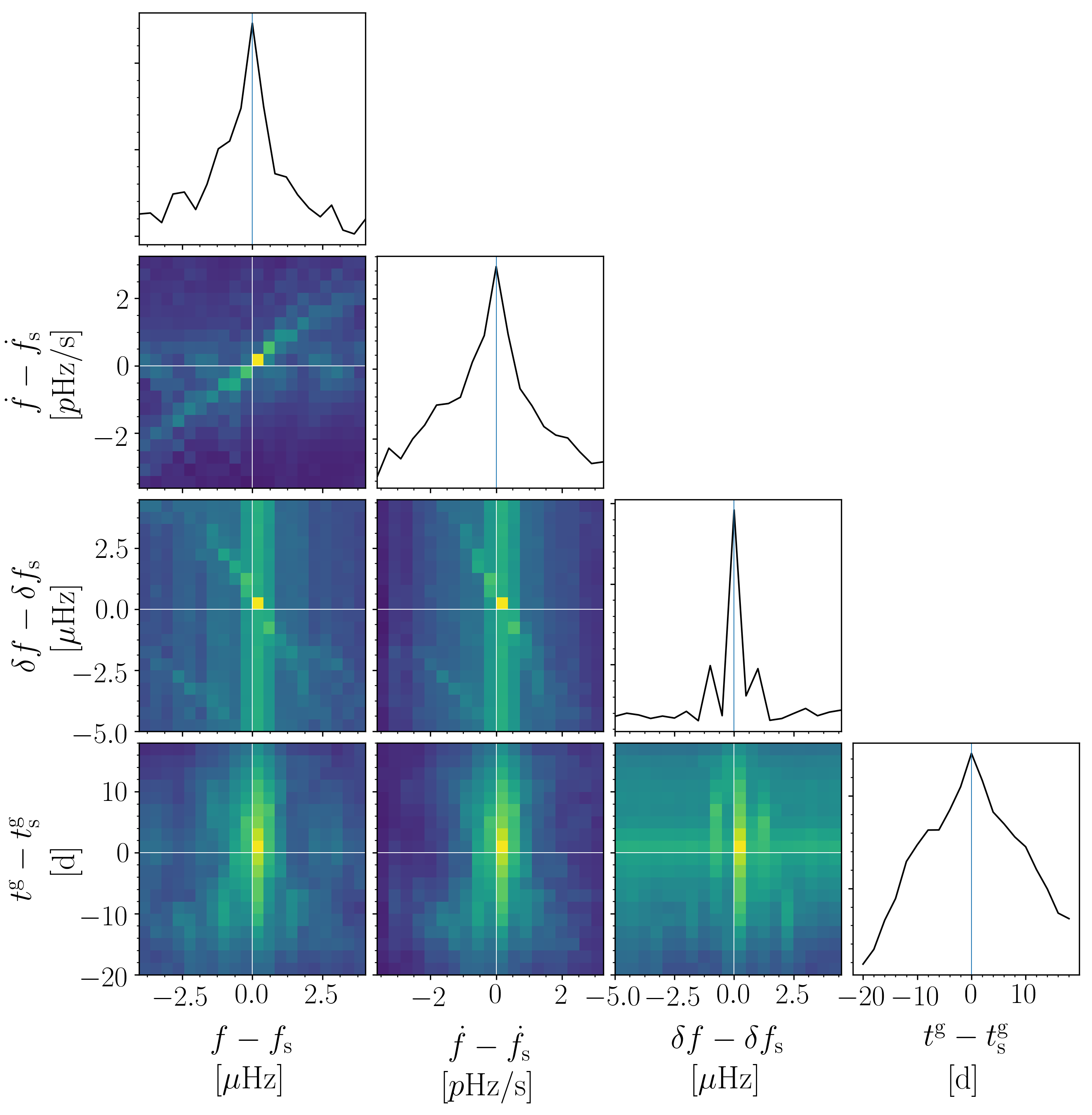
Figure 1: Grid-corner plot showing various marginalizations of the glitch-robust semicoherent ${\mathcal{F}}$-statistic computed using a grid-based search over the prior ranges in Table 2. Solid lines indicate the simulated signal parameters.

Table 2: Priors used for the search parameters; the subscript s indicates the simulation values given in Table 1 and $t^{\rm g}$ is defined from the start of the observation span. For the uncertainty in $f$ and $\dot{f}$, the number of fully coherent unit-mismatch templates is $\mathcal{N}^{*}=1000$.

		Uniform prior range
$f$	$\sim$	$f_{s}\pm 4.0\times 10^{-6}$ Hz
$\dot{f}$	$\sim$	$\dot{f}_{s}\pm 1.8\times 10^{-12}$ Hz/s
$\delta f$	$\sim$	$[0,5\times 10^{-5}]$ Hz
$t^{\rm g}$	$\sim$	$[5,45]$ days

The grid spacing in this instance is sufficiently fine to provide reasonably good parameter estimation. For detection purposes it may even suffice to have sparser template coverage in the glitch time (where the signal appears quite wide compared to the prior range). At a fixed computing cost, this would allow for denser coverage in other parameters where the signal is narrower compared to the prior range.

III.4 MCMC-based glitch-robust search

Figure 2: Corner plot showing various marginalizations of the exponential of the glitch-robust semicoherent ${\mathcal{F}}$-statistic computed using an MCMC-based search. Solid lines indicate the simulated signal parameters while dashed lines (on the one-dimensional histograms) indicate 1-$\sigma$ quantiles. Figure generated using the corner (Foreman-Mackey, 2016) package.

MCMC-based standard-CW searches have already been used with success (Christensen et al., 2004; Veitch, 2007; Umstätter et al., 2004; Abbott et al., 2010). Recently we demonstrated (Ashton and Prix, 2018) that this success relies on the size of the parameter space being sufficiently small, as quantified by $\mathcal{N}^{*}$. Namely it was found that typically $\mathcal{N}^{*}\lesssim 1000$ is a good guideline, but this can depend on the exact MCMC setup. For too-large parameter spaces, the MCMC algorithm tends to fail to converge to the signal peak in a reasonable amount of time.

For the follow-up of candidates from wide-parameter space searches, the size of the phase-evolution parameter space (i.e., the candidate uncertainty) is well constrained (or, this can be ensured by performing a refinement step). It is not possible to calculate $\mathcal{N}^{*}$ for a glitch-robust detection statistic without the metric. However, in practice, we find that for typical glitch size and rates seen in the pulsar population (Ashton and Prix, 2018; Fuentes et al., 2017) and typical observing spans, an MCMC-based glitch-robust search is effective at converging on simulated signals. For longer observing spans (or if allowing for larger glitches than those observed in the pulsar population) further work will need to be carried out to ensure the method is robust.

The advantage of an MCMC-based, instead of a grid-based, approach is that there is no requirement to predetermine the grid points. In effect, the ensemble MCMC sampler adapts to the topology of the maxima during the burn-in phase (for a more detailed overview of MCMC-based CW search methods see Ashton and Prix (2018)).

To illustrate the results of an MCMC search, we run it on the same data set used to produce Fig. 1 (simulation properties are given in Table 1) with the same uniform priors, as given in Table 2. In Fig. 2 we plot the resulting corner plot.

MCMC searches produce samples from the posterior, which, if the signal is successfully identified, usually occupies only a small fraction of the prior range. As a result, an MCMC search does not produce a posterior over the whole prior range, but only over the region of interest. As a consequence of this the range shown in Fig. 1 is much larger than that of Fig. 2: the latter shows the range of the posterior peak only while the former shows the entire prior range. Moreover, we note that in Fig. 1 for the grid-based search we plot the ${\mathcal{F}}$-statistic, corresponding to the (marginalized) log-likelihood ratio. On the other hand, in Fig. 2 for the MCMC-based search we plot the estimated posterior which in this instance, where we use uniform priors, is proportional to the likelihood, corresponds to the exponential of the ${\mathcal{F}}$-statistic. This is why the peak looks much narrower compared to Fig. 1 while showing in principle the same likelihood-function.

III.5 Comparing grid- and MCMC-based searches

In order to provide a simple comparison between grid- and MCMC-based searches, we run a Monte-Carlo study. We produce 500 data sets containing a simulated signal with a single glitch in Gaussian noise. Such a signal, perfectly matched, has a predicted $\widetilde{2{\mathcal{F}}}$ of approximately $330$. The noise, amplitude and standard phase evolution parameters are given in Table 1, except that we jitter the frequency and spin-down, picking their value uniformly from within the inner half of the prior region given in Table 2. We also select the glitch epoch from the distribution given in this table. Meanwhile, for the glitch magnitude, we sample from the observed pulsar population distribution (Ashton et al., 2017); while the aim of the section is to compare search methods, this choice of simulation distribution allows us to also verify that the naive priors are robust to a more astrophysically motivated population distribution.

Varying the required computation time (for the grid-based search, by varying the number of grid points; for the MCMC-based search, by varying the number of steps taken), in Fig. 3 we plot the relative difference between the recovered maximum $\widehat{2{\mathcal{F}}}$ (for each method) and $\widehat{2{\mathcal{F}}}_{\mathrm{inject}}=\widehat{2{\mathcal{F}}}(\boldsymbol{\mathbf{\lambda}}_{s})$, the statistic measured at the simulated signal parameters $\boldsymbol{\mathbf{\lambda}}_{s}$. Due to the presence of noise, the actual maximum $\widehat{2{\mathcal{F}}}$ will typically not occur at the signal parameters $\boldsymbol{\mathbf{\lambda}}_{s}$ but be slightly offset and we therefore generally expect the maximum recovered $\widehat{2{\mathcal{F}}}>\widehat{2{\mathcal{F}}}_{\mathrm{inject}}$, provided the search method manages to localize the maximum $\widehat{2{\mathcal{F}}}$ well enough.

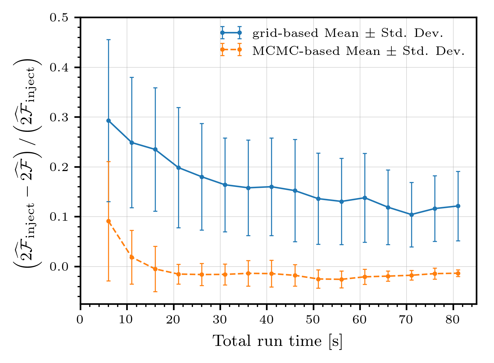
Figure 3: Comparison of the relative maximum $\widehat{2{\mathcal{F}}}$ found by each method compared to $\widehat{2{\mathcal{F}}}_{\mathrm{inject}}$, the value calculated at the simulated signal parameters $\boldsymbol{\mathbf{\lambda}}_{s}$. All timings performed on an Intel® Core™ i7-7820HQ CPU @ 2.90GHz processor.

From this figure, it is evident that at the same run-time, the MCMC-based search outperforms the grid-based search, with the majority of points finding a larger detection statistic than $\widehat{2{\mathcal{F}}}_{\mathrm{inject}}$. This is to be expected since the MCMC search is operating optimally (i.e., the size of parameter space is sufficiently small). As such, the MCMC quickly converges to the maximum while a grid-based search spends most of the computing time calculating the detection statistic for points not near to the signal peak. For added context, Figs 1 and 2 both have an approximate run-time of 90s; for the grid-based search, the peak is only sampled a handful of times yet almost all of the MCMC samples (by design) come from the peak.

IV Glitching vs. standard-CW Bayes factor

We now discuss how to quantify whether a signal is glitching and how many glitches best explain the data. We do this using a Bayes factor, the ratio of likelihoods for data $\boldsymbol{x}$ under two hypotheses. If $\mathcal{H}_{\rm N}$ implies that the data contains only Gaussian noise while $\mathcal{H}_{\rm S}$ implies that it contains an CW signal in addition to noise, then

$$B_{\rm S/N}(\boldsymbol{x})\equiv\frac{P(\boldsymbol{x}|\mathcal{H}_{\rm S})}{P(\boldsymbol{x}|\mathcal{H}_{\rm N})}\,.$$ (7)

It can be shown (Prix and Krishnan, 2009; Prix et al., 2011; Ashton and Prix, 2018) that the signal vs. noise Bayes factor at fixed phase-evolution parameters $\boldsymbol{\mathbf{\lambda}}$ is

$$B_{\rm S/N}(\boldsymbol{x};\boldsymbol{\mathbf{\lambda}},N)=\left(\frac{70}{\hat{\rho}_{\mathrm{max}}^{4}}\right)^{N}e^{\hat{{\mathcal{F}}}(\boldsymbol{x};\boldsymbol{\mathbf{\lambda}},N)}\,,$$ (8)

where $\hat{{\mathcal{F}}}(\boldsymbol{x};\boldsymbol{\mathbf{\lambda}},N)$ is the $N$-segment semicoherent ${\mathcal{F}}$-statistic defined in Eq. (3) and $\hat{\rho}_{\mathrm{max}}$ is an arbitrary upper cutoff on the prior range in signal strength (Prix et al., 2011).

Similarly, defining $\mathcal{H}_{\rm gS}$ as the glitching-signal hypothesis, we see that the targeted (in the sense that it depends on the model parameter) glitching-signal vs. noise Bayes factor is

$$\begin{split}B_{\rm gS/N}\left(\boldsymbol{x};\boldsymbol{\mathbf{\lambda}},\{\!\!\{\delta f^{(k)}_{\ell}\}\!\!\},\{t^{\rm g}_{\ell}\},N_{\rm g}\right)&\\ &\equiv\left(\frac{70}{\hat{\rho}_{\mathrm{max}}^{4}}\right)^{N_{\rm g}+1}e^{\hat{{\mathcal{F}}}\left(\boldsymbol{x};\boldsymbol{\mathbf{\lambda}},\{\!\!\{\delta f^{(k)}_{\ell}\}\!\!\},\{t^{\rm g}_{\ell}\}\right)}\,,\end{split}$$ (9)

where the exponent is the glitch-robust semicoherent ${\mathcal{F}}$-statistic, defined in Eq. (4).

After marginalizing the targeted Bayes factor we get the signal vs. noise Bayes factor; i.e., for the standard search,

$$B_{\rm S/N}(\boldsymbol{x};N)=\int B_{\rm S/N}(\boldsymbol{x};\boldsymbol{\mathbf{\lambda}},N)P(\boldsymbol{\mathbf{\lambda}}|\mathcal{H}_{\rm S})d\boldsymbol{\mathbf{\lambda}},$$ (10)

while for the semicoherent glitch-robust

$$\begin{split}B_{\rm gS/N}(\boldsymbol{x};N_{\rm g})&=\int B_{\rm S/N}\left(\boldsymbol{x};\boldsymbol{\mathbf{\lambda}},\{\!\!\{\delta f^{(k)}_{\ell}\}\!\!\},\{t^{\rm g}_{\ell}\},N_{\rm g}\right)\times\\ &\hskip 25.60747ptP\left(\boldsymbol{\mathbf{\lambda}},\{\!\!\{\delta f^{(k)}_{\ell}\}\!\!\},\{t^{\rm g}_{\ell}\}|\mathcal{H}_{\rm S}\right)\\ &\hskip 25.60747ptd\boldsymbol{\mathbf{\lambda}}d\{\!\!\{\delta f^{(k)}_{\ell}\}\!\!\}d\{t^{\rm g}_{\ell}\}\,.\end{split}$$ (11)

The arbitrary prior cutoff $\hat{\rho}_{\mathrm{max}}$ makes it difficult to interpret either of these Bayes factors by themselves: one can tune the Bayes factor by arbitrary changes in the prior. However, if we define

$$B_{\rm gS/S}(\boldsymbol{x},N_{\rm g})\equiv\frac{B_{\rm gS/N}(\boldsymbol{x},N_{\rm g})}{B_{\rm S/N}(\boldsymbol{x},N=N_{\rm g}+1)}\,,$$ (12)

the glitching-CW vs. standard-CW Bayes factor, then the arbitrary prior cutoff cancels and we are left with an interpretable Bayes factor for whether the signal is glitching or not.

Calculation of the Bayes factor can be done by either a grid-based (using numerical integration of a dense sampling of the posterior) or MCMC-based method (using thermodynamic integration (Goggans and Chi, 2004)). In future, we intend to extend the functionality to include nested sampling (Skilling, 2006) which will improve the robustness of the evidence calculation (see, e.g., Ref. (Allison and Dunkley, 2014) for a comparison).

To understand the behaviour of $B_{\rm gS/S}(\boldsymbol{x},N_{\rm g})$ as a function of the glitch magnitude, we run a Monte Carlo study, simulating 100 data sets (for each $\delta f$) with a glitching signal in Gaussian noise. We use the parameters given in Table 1, except $\delta f$ which we vary systematically over a relevant domain. For each data set, we run a glitch-robust semicoherent MCMC search with $N_{\rm g}=1$ along with a semicoherent MCMC search with $N=2$ and calculate the resulting Bayes factor. The MCMC parameters are chosen such that the log Bayes factors are estimated to within a few percent. In Fig. 4 we plot the mean and standard deviation calculated over all data sets. We see that for small glitches, the Bayes factor prefers the standard signal hypothesis. But, once glitches are sufficiently large, the glitching-signal hypothesis is preferred.

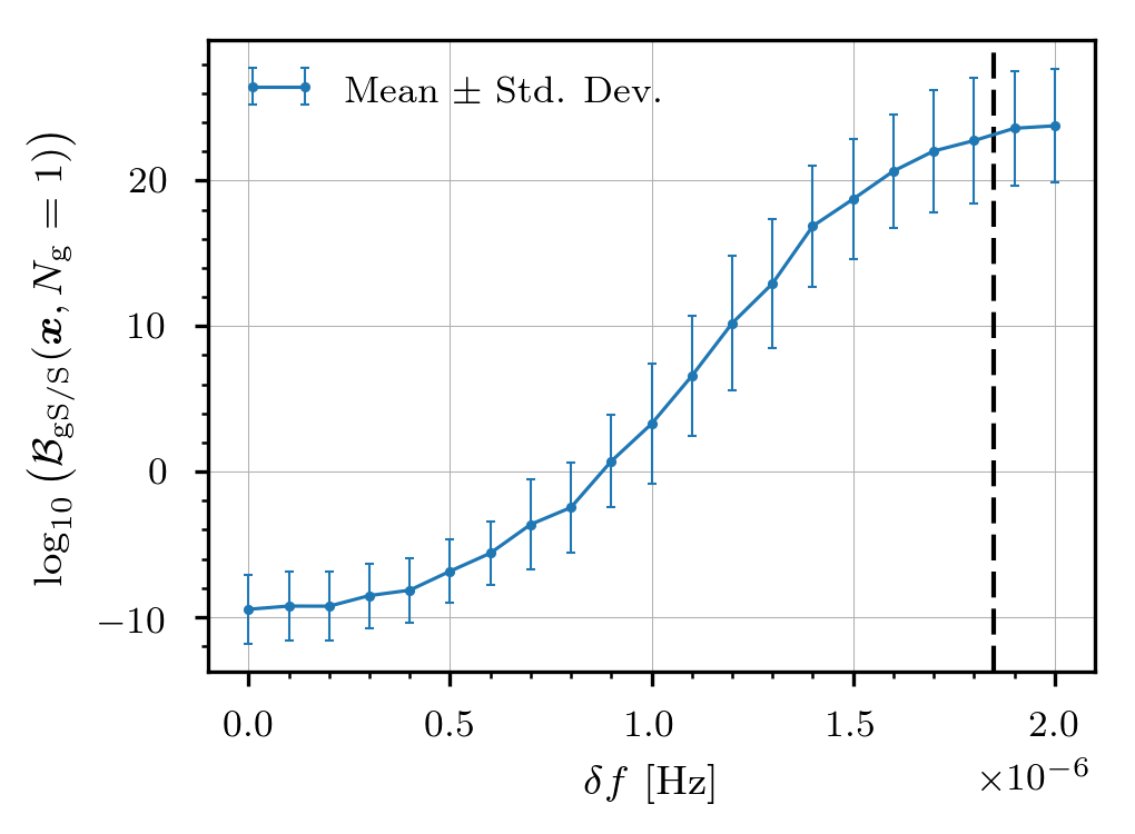
Figure 4: Monte Carlo study of the $B_{\rm gS/S}(\boldsymbol{x},N_{\rm g}=1)$ Bayes factor as a function of the simulated glitch magnitude. A dashed vertical line indicates the value of Eq. (13) for the 50-day duration used in this study.

To determine the preferred number of glitches, $B_{\rm gS/S}(\boldsymbol{x},N_{\rm g})$ can be calculated for different $N_{\rm g}$ and interpreted as a posterior over $N_{\rm g}$. Large numbers of glitches, $\gtrsim 10$ say, may be difficult to handle and require some tuning of the MCMC sampler.

Fig. 4 illustrates that the glitch-robust search (as a function of the glitch size) plateaus above a certain minimum glitch size. An approximate way to characterize this size is to use the averaged (over glitch-time) single-glitch metric mismatch expressions derived in Ashton et al. (2017). Note that this is the metric for a standard CW search of a glitching signal and not the metric for the glitch-robust statistic introduced in Sec II. For example, for a fully coherent search at a fixed sky-location over frequency and spin-down, the minimum average metric mismatch is given by $\tilde{\mu}=(\pi T\delta f)^{2}/630$. Setting the metric-mismatch to unity and inverting gives

$$\delta f=\frac{\sqrt{630}}{\pi T}\,,$$ (13)

a rough order-of-magnitude estimate of the glitch size for which a standard-CW search would be sufficiently affected by the glitch that the glitch hypothesis will be preferred. Similar results can be derived for jumps in higher-order frequency spin-downs using the corresponding components of the glitch metric.

In Fig. 4, we plot the value of Eq. (13), given the 50-day duration of data used. Notably, this agrees with the point at which the Bayes factor begins to plateau.

V Identifying glitching signal in standard searches

In order to identify when a signal candidate from a standard-CW semicoherent search might best be followed up using a glitch-robust method, we now discuss the behaviour of glitching signals in a standard-CW search.

V.1 Multiple modes

One indicator of a glitching signal in a standard-CW search is the existence of multiple peaks in the detection statistic resulting from the template matching different parts of the signals. How exactly this behaviour manifests depends on the magnitude and size of the glitches, the data span, and the search setup.

Considering a signal which undergoes a single glitch with a jump $\{\delta f^{(k)}\}$, we can identify two limiting cases depending on whether the glitch size is smaller or larger than a critical glitch size $\delta f^{(k)}_{c}$ : if $\delta f^{(k)}\ll\delta f^{(k)}_{c}$, the effect of the glitch is negligible within the search setup; if instead, $\delta f^{(k)}\gg\delta f^{(k)}_{c}$, the signal can be thought of as two transient CWs, and we will find two distinct peaks in the detection statistic corresponding to the pre- and post-glitch signal parameters. Between these two extremes, when $\delta f^{(k)}\sim\delta f^{(k)}_{c}$, the resulting structure in the detection statistic can be quite complicated. If required, the critical glitch size can be estimated from the single-glitch metric mismatches derived in Ashton et al. (2017).

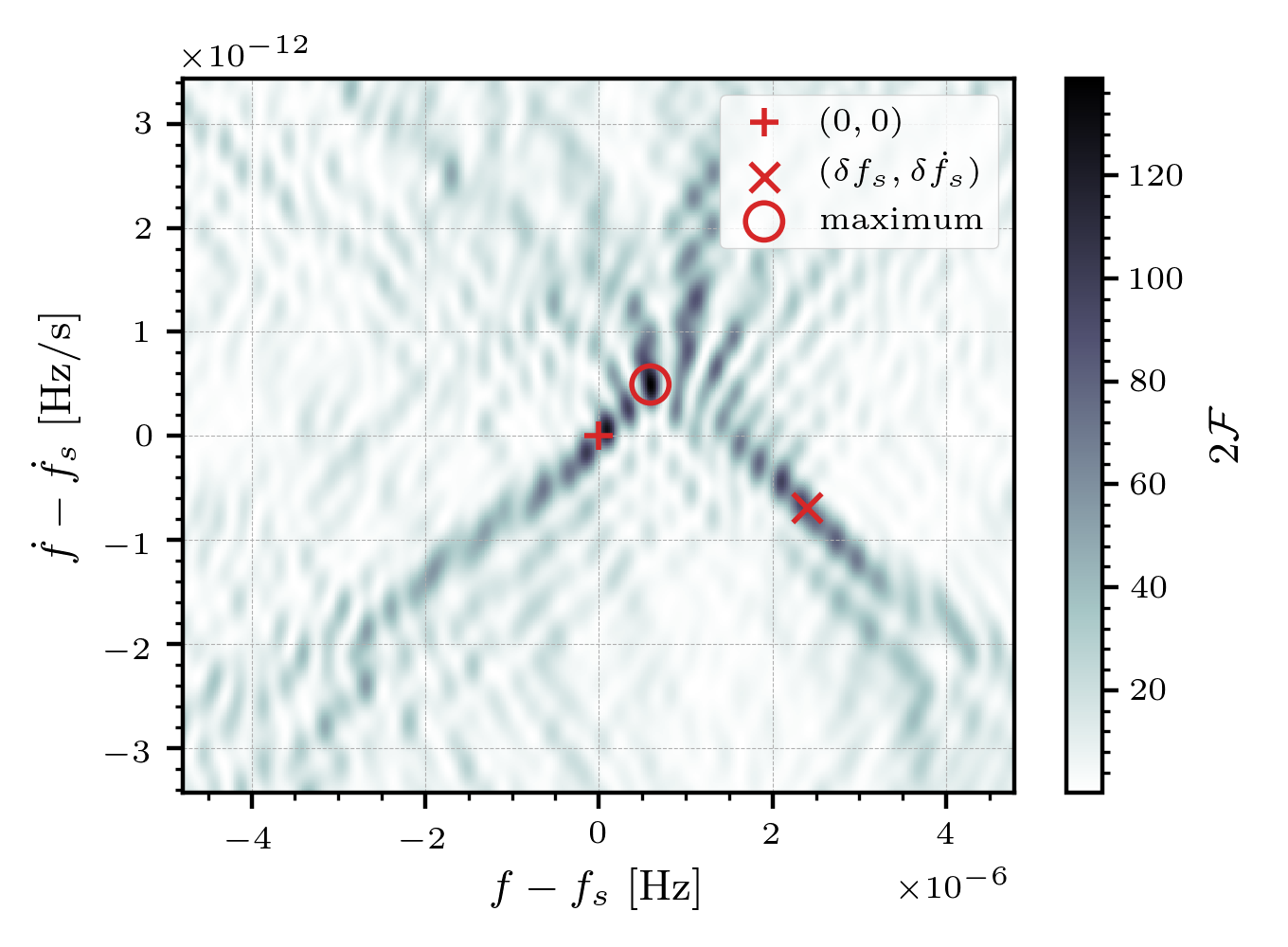
Figure 5: The fully coherent $\widetilde{2{\mathcal{F}}}$ computed over a grid in $f$ and $\dot{f}$ for the simulated glitching signal.

In order to illustrate this intermediate case, in Fig. 5 we show a standard-CW fully coherent grid search over frequency and spin-down for a simulated glitching signal. The simulation properties are given in Table 1, except that we set $\delta f=$2.4\text{\times}{10}^{-6}\text{\,}\mathrm{H}\mathrm{z}$$ and $\delta\dot{f}=$-6.9\text{\times}{10}^{-13}\text{\,}\mathrm{H}\mathrm{z}\mathrm{/}\mathrm{s}$$. As the reference time and glitch time coincide, for the fully coherent search, the pre-glitch frequency and derivative is $f_{s}$, $\dot{f}_{s}$ while the post-glitch frequency and derivative are $f_{s}+\delta f$, $\dot{f}_{s}+\delta\dot{f}$. Two distinct ellipsoid patterns can be observed centered on the locations of the pre and post-glitch signals, but the maximum does not coincide with either.

Having multiple peaks in the frequency and its derivatives might be expected, but we typically also find multiple peaks in the sky position, even though the sky position of the source does not vary over a glitch. This is because by allowing the sky position to vary, the standard template fit to the glitching signal can be improved; this can happen in multiple ways, resulting in multiple peaks and will in general result in biases in the recovered sky position.

V.2 Sliding windows

A sliding window can be another simple, but powerful diagnostic test for a glitching signal. Fixing all other values to those of the maximum posterior estimate (or a set of parameters sufficiently close to the peak), the detection statistic is computed for a range of frequencies in an overlapping sliding time-window over the total data span. One could also do this for the frequency derivative (or any other parameter). Stacking the results together into a colour plot, if the signal is sufficiently strong, the glitch can easily be discerned from the change in frequency. We provide an example in Fig. 6 using the same data set used to produce Fig. 5.

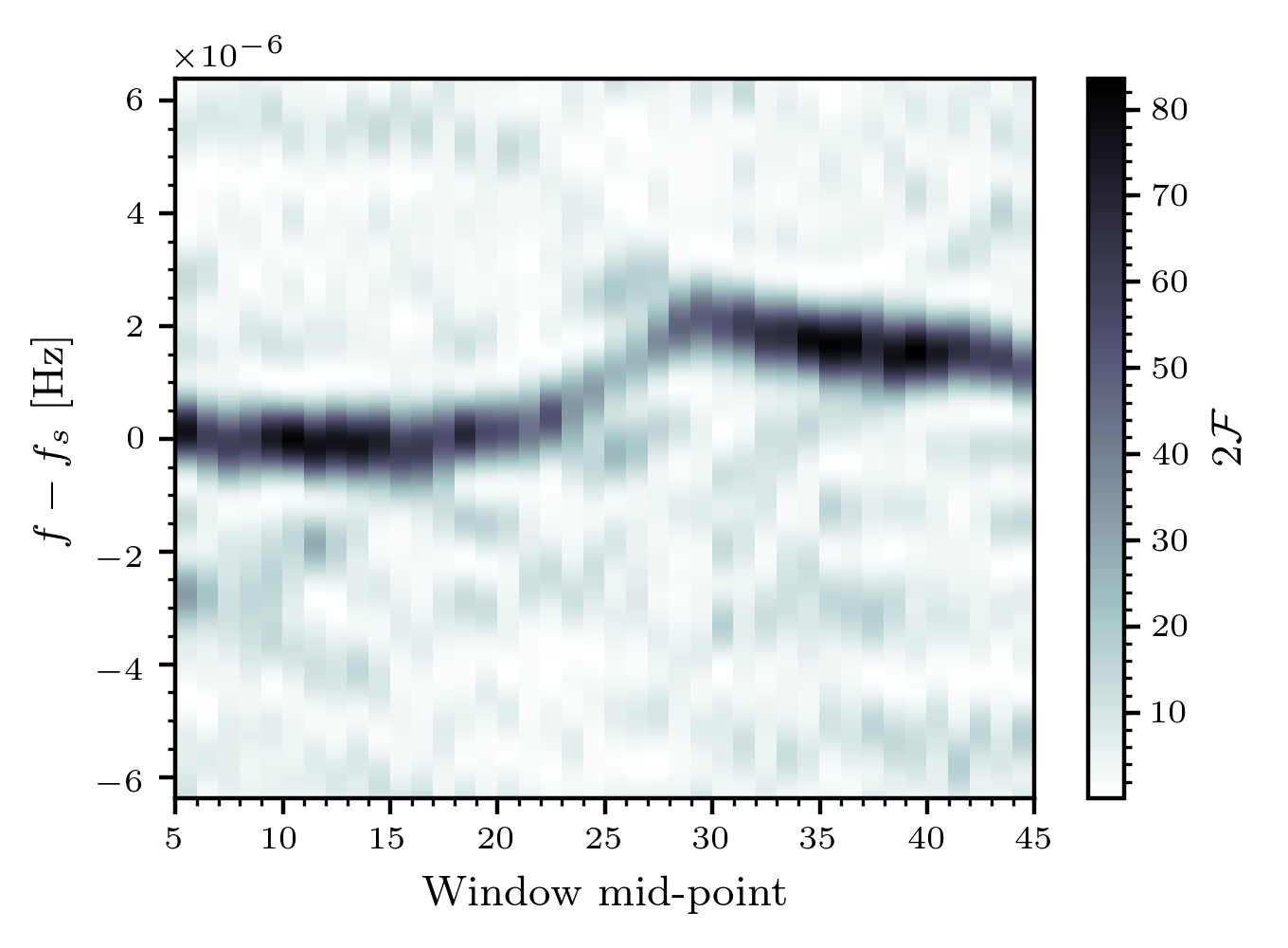
Figure 6: Illustration of the frequency sliding-window, a useful diagnostic tool for identifying glitching signals. In this example, a 10-day window is slid in increments of 1 day.

VI Discussion

We have described a semicoherent glitch-robust detection statistic for use in evaluating if candidates found in wide-parameter space searches are glitching signals. This simple method adapts standard search routines, using a signal model that includes glitches as a set of instantaneous changes in the frequency and higher-order spin-downs at a set of glitch epochs.

Comparing grid- and MCMC-based search methods, we find that the MCMC-based search is a superior method for performing glitch-robust searches of candidates from wide-parameter space searches. For the same computing cost it is able to better identify the maximum and perform parameter estimation vital to interpretation. MCMC-based glitch-robust searches are, for a suitable candidate uncertainty level, computationally cheap to run and provide parameter estimation and evidence estimates. Moreover, an MCMC-based method does not require a pre-specified grid template. We therefore recommend that such glitch-robust MCMC-based methods be used in the follow-up of candidates identified in wide-parameter searches.

The methods introduced in this paper have been implemented in the package pyfstat (Ashton and Keitel, 2018). Source code along with all examples in this work can be found at https://gitlab.aei.uni-hannover.de/GregAshton/PyFstat.

VII Acknowledgements

The authors kindly thank the members of the Continuous Waves group of the LIGO Scientific Collaboration and the Virgo Scientific Collaboration for useful feedback and discussion during the development of this work. We thank Sylvia Zhu for cogent and useful comments during the preparation of the manuscript. DIJ acknowledges funding from STFC through grant number ST/M000931/1. This article has been assigned the document number LIGO-P1800057.

References

- Abbott et al. (2017a) B. P. Abbott, R. Abbott, T. D. Abbott, F. Acernese, K. Ackley, C. Adams, T. Adams, P. Addesso, R. X. Adhikari, V. B. Adya, and et al., “All-sky search for periodic gravitational waves in the O1 LIGO data,” Phys. Rev. D 96, 062002 (2017a), arXiv:1707.02667 [gr-qc] .
- Abbott et al. (2017b) B. P. Abbott, R. Abbott, T. D. Abbott, F. Acernese, K. Ackley, C. Adams, T. Adams, P. Addesso, R. X. Adhikari, V. B. Adya, and et al., “First low-frequency Einstein@Home all-sky search for continuous gravitational waves in Advanced LIGO data,” Phys. Rev. D 96, 122004 (2017b), arXiv:1707.02669 [gr-qc] .
- Hobbs et al. (2010) G. Hobbs, A. G. Lyne, and M. Kramer, “An analysis of the timing irregularities for 366 pulsars,” Mon. Notices Royal Astron. Soc. 402, 1027–1048 (2010), arXiv:0912.4537 .
- Espinoza et al. (2011) C. M. Espinoza, A. G. Lyne, B. W. Stappers, and M. Kramer, “A study of 315 glitches in the rotation of 102 pulsars,” Mon. Notices Royal Astron. Soc. 414, 1679–1704 (2011), arXiv:1102.1743 [astro-ph.HE] .
- Fuentes et al. (2017) J. R. Fuentes, C. M. Espinoza, A. Reisenegger, B. Shaw, B. W. Stappers, and A. G. Lyne, “The glitch activity of neutron stars,” Astron. Astrophys. 608, A131 (2017), arXiv:1710.00952 [astro-ph.HE] .
- Jones (2004) D. I. Jones, “Is timing noise important in the gravitational wave detection of neutron stars?” Phys. Rev. D 70, 042002 (2004), arXiv:0406045 [gr-qc] .
- Ashton et al. (2015) G. Ashton, D. I. Jones, and R. Prix, “Effect of timing noise on targeted and narrow-band coherent searches for continuous gravitational waves from pulsars,” Phys. Rev. D 91, 062009 (2015), arXiv:1410.8044 [gr-qc] .
- Ashton et al. (2017) G. Ashton, R. Prix, and D. I. Jones, “Statistical characterization of pulsar glitches and their potential impact on searches for continuous gravitational waves,” Phys. Rev. D 96, 063004 (2017), arXiv:1704.00742 [gr-qc] .
- Prix (2009) R. Prix, “Gravitational Waves from Spinning Neutron Stars,” in Astrophysics and Space Science Library, Astrophysics and Space Science Library, Vol. 357, edited by W. Becker (2009) p. 651, https://dcc.ligo.org/LIGO-P060039/public.
- Jaranowski et al. (1998) P. Jaranowski, A. Królak, and B. F. Schutz, “Data analysis of gravitational-wave signals from spinning neutron stars: The signal and its detection,” Phys. Rev. D 58, 063001 (1998), gr-qc/9804014 .
- Edwards et al. (2006) R. T. Edwards, G. B. Hobbs, and R. N. Manchester, “TEMPO2, a new pulsar timing package - II. The timing model and precision estimates,” Mon. Notices Royal Astron. Soc. 372, 1549–1574 (2006), astro-ph/0607664 .
- Prix and Krishnan (2009) R. Prix and B. Krishnan, “Targeted search for continuous gravitational waves: Bayesian versus maximum-likelihood statistics,” Class. Quantum Grav. 26, 204013 (2009), arXiv:0907.2569 [gr-qc] .
- Prix et al. (2011) R. Prix, S. Giampanis, and C. Messenger, “Search method for long-duration gravitational-wave transients from neutron stars,” Phys. Rev. D 84, 023007 (2011), arXiv:1104.1704 [gr-qc] .
- Gelman et al. (2013) A. Gelman, J. B. Carlin, H. S. Stern, D. B. Dunson, A. Vehtari, and D. B. Rubin, Bayesian Data Analysis, 3rd ed. (CRC Press, 2013).
- Archibald et al. (2013) R. F. Archibald, V. M. Kaspi, C.-Y. Ng, K. N. Gourgouliatos, D. Tsang, P. Scholz, A. P. Beardmore, N. Gehrels, and J. A. Kennea, “An anti-glitch in a magnetar,” Nature (London) 497, 591–593 (2013), arXiv:1305.6894 [astro-ph.HE] .
- Livingstone et al. (2009) M. A. Livingstone, S. M. Ransom, F. Camilo, V. M. Kaspi, A. G. Lyne, M. Kramer, and I. H. Stairs, “X-ray and Radio Timing of the Pulsar in 3C 58,” Astrophys. J. 706, 1163–1173 (2009), arXiv:0901.2119 [astro-ph.SR] .
- Prix (2007) R. Prix, “Template-based searches for gravitational waves: efficient lattice covering of flat parameter spaces,” Class. Quantum Grav. 24, S481–S490 (2007), arXiv:0707.0428 [gr-qc] .
- Wette and Prix (2013) K. Wette and R. Prix, “Flat parameter-space metric for all-sky searches for gravitational-wave pulsars,” Phys. Rev. D 88, 123005 (2013), arXiv:1310.5587 [gr-qc] .
- Wette (2015) K. Wette, “Parameter-space metric for all-sky semicoherent searches for gravitational-wave pulsars,” Phys. Rev. D 92, 082003 (2015), arXiv:1508.02372 [gr-qc] .
- Ashton and Prix (2018) G. Ashton and R. Prix, “Hierarchical multi-stage MCMC follow-up of continuous gravitational wave candidates,” ArXiv e-prints (2018), arXiv:1802.05450 [astro-ph.IM] .
- Foreman-Mackey (2016) Daniel Foreman-Mackey, “corner.py: Scatterplot matrices in python,” The Journal of Open Source Software 24 (2016), 10.21105/joss.00024.
- Christensen et al. (2004) N. Christensen, R. J. Dupuis, G. Woan, and R. Meyer, “Metropolis-Hastings algorithm for extracting periodic gravitational wave signals from laser interferometric detector data,” Phys. Rev. D 70, 022001 (2004), gr-qc/0402038 .
- Veitch (2007) J. D. Veitch, Applications of Markov Chain Monte Carlo methods to continuous gravitational wave data analysis, Ph.D. thesis, University of Glasgow (2007).
- Umstätter et al. (2004) R. Umstätter, R. Meyer, R. J. Dupuis, J. Veitch, G. Woan, and N. Christensen, “Estimating the parameters of gravitational waves from neutron stars using an adaptive MCMC method,” Class. Quantum Grav. 21, S1655–S1665 (2004).
- Abbott et al. (2010) B. P. Abbott, R. Abbott, F. Acernese, R. Adhikari, P. Ajith, B. Allen, G. Allen, M. Alshourbagy, R. S. Amin, S. B. Anderson, and et al., “Searches for Gravitational Waves from Known Pulsars with Science Run 5 LIGO Data,” Astrophys. J. 713, 671–685 (2010), arXiv:0909.3583 [astro-ph.HE] .
- Goggans and Chi (2004) P. M. Goggans and Y. Chi, “Using thermodynamic integration to calculate the posterior probability in bayesian model selection problems,” AIP Conference Proceedings 707, 59–66 (2004).
- Skilling (2006) John Skilling, “Nested sampling for general bayesian computation,” Bayesian analysis 1, 833–859 (2006).
- Allison and Dunkley (2014) R. Allison and J. Dunkley, “Comparison of sampling techniques for Bayesian parameter estimation,” Mon. Notices Royal Astron. Soc. 437, 3918–3928 (2014), arXiv:1308.2675 [astro-ph.IM] .
- Ashton and Keitel (2018) G. Ashton and D. Keitel, “PyFstat-v1.2,” (2018), https://doi.org/10.5281/zenodo.1243931.