Computational tools for solving a marginal problem with applications in Bell non-locality and causal modeling

Abstract

Marginal problems naturally arise in a variety of different fields: basically, the question is whether some marginal/partial information is compatible with a joint probability distribution. To this aim, the characterization of marginal sets via quantifier elimination and polyhedral projection algorithms is of primal importance. In this work, before considering specific problems, we review polyhedral projection algorithms with focus on applications in information theory, and, alongside known algorithms, we also present a newly developed geometric algorithm which walks along the face lattice of the polyhedron in the projection space. One important application of this is in the field of quantum non-locality, where marginal problems arise in the computation of Bell inequalities. We apply the discussed algorithms to discover many tight entropic Bell inequalities of the tripartite Bell scenario as well as more complex networks arising in the field of causal inference. Finally, we analyze the usefulness of these inequalities as nonlocality witnesses by searching for violating quantum states.

I Introduction

Starting point of this paper is the marginal problem: given joint distributions of certain subsets of random variables $X_{1},\dots,X_{n}$, are they compatible with the existence of any joint distribution for all these variables? In other words, is it possible to find a joint distribution for all these variables, such that this distribution marginalizes to the given ones? Such a problem naturally arises in several different fields. From the classical perspective, applications of the marginal problem range, just to cite a few examples, from knowledge integration in artificial intelligence and database theory Studenỳ (1994); Lauritzen and Spiegelhalter (1988) to causal discovery Pearl (2009); Spirtes et al. (2001) and network coding protocols Yeung (2008). Within quantum information perhaps the most famous example –the one that will be the main focus in this paper– is the phenomenon of nonlocality Bell (1964), showing that quantum predictions for experiments performed by distant parties are at odds with the assumption of local realism.

As shown by Bell in his seminal paper Bell (1964), the assumption of local realism imposes strict constraints on the possible probability distributions that are compatible with it. These are the famous Bell inequalities that play a fundamental role in the understanding of nonlocality since it is via their violation that we can unambiguously probe the nonlocal character of quantum correlations. Given its importance, very general frameworks have been developed for the derivation of Bell inequalities Pitowsky (1989); Brunner et al. (2014). Unfortunately, however, finding all Bell inequalities is a very hard problem given that its computational complexity increases very fast as the scenario of interest becomes less simple Pitowsky (1989, 1991). The situation is even worse for the study of nonlocality in complex quantum networks, where on the top of local realism one also imposes additional constraints Branciard et al. (2010, 2012); Fritz (2012); Tavakoli et al. (2014); Chaves et al. (2015a); Chaves (2016); Tavakoli (2016); Lee and Spekkens (2015); Wolfe et al. (2016); Carvacho et al. (2017); Andreoli et al. (2017). In this case, the derivation of Bell inequalities involves the characterization of complicated non-convex sets for which even more computationally demanding tools from algebraic geometry Geiger and Meek (1999); Garcia et al. (2005); Chaves (2016); Lee and Spekkens (2015) seem to be the only viable alternative.

In order to circumvent some these issues, an alternative route that has been attracting growing attention lately is the one given by entropic Bell inequalities Braunstein and Caves (1988); Cerf and Adami (1997); Chaves and Fritz (2012); Fritz (2012); Fritz and Chaves (2013); Chaves (2013); Chaves et al. (2014a); Henson et al. (2014); Kurzyński and Kaszlikowski (2014); Poh et al. (2015); Chaves and Budroni (2016); Weilenmann and Colbeck (2016a, b); Budroni et al. (2016); Weilenmann and Colbeck (2017); Miklin et al. (2017); Pienaar (2017). In this case, rather than asking if a given probability distribution is compatible or not with local realism, we ask the same question but for the Shannon entropies of such distributions. The novelty of the entropic approach have both conceptual and technical reasons. Entropy is a key concept in our understanding of information theory, thus having a framework that focuses on it naturally leads to new insights and applications Pawłowski et al. (2009); Short and Wehner (2010); Dahlsten et al. (2012); Barnum et al. (2010); Fritz (2012); Henson et al. (2014); Chaves et al. (2015b, c). In turn, entropies allow for a much simpler and compact characterization of Bell inequalities –at the cost of not being a complete description– in a variety of scenarios, most notably in the aforementioned quantum networks Chaves et al. (2014a); Henson et al. (2014); Chaves et al. (2015b); Chaves and Budroni (2016); Weilenmann and Colbeck (2017); Miklin et al. (2017); Pienaar (2017). Not surprisingly, however, this approach is also hampered by computational complexity issues. As will be discussed in details through this paper, current methods for the derivation of entropic Bell inequalities (see for instance Budroni and Cabello (2012); Chaves et al. (2014a); Henson et al. (2014); Chaves and Budroni (2016); Weilenmann and Colbeck (2016b, 2017); Miklin et al. (2017) mostly rely on quantifier elimination algorithms Williams (1986) that in practice is limited to a few simple cases of interest.

Within this context the aim of this paper is three-fold. First, to review existing methods for solving the marginal problem, particularly those relevant for the derivation of Bell inequalities. Given the importance of it, not surprisingly there is a rich literature and methods aiming at its solution Duffin (1974); Williams (1986); Huynh et al. (1990); Davenport and Heintz (1988); Lassez (1990); Lassez and Lassez (1990); Huynh et al. (1992); Imbert (1993); Simon and King (2005); Jones et al. (2004). Most of these results, however, appear in quite diverse contexts and most prominently in the field of convex optimization and computer science. Thus, we hope that researchers on quantum information and in particular working on Bell nonlocality will benefit from the concise and unified exposition of the computational tools that we present here. Our second aim is to give our own contribution by developing new computational tools that complement and in some case improve existing algorithms. That is of particular relevance to our third and final aim with this paper: to apply our improved method to derive new tests for witnessing quantum nonlocality. Here we limit ourselves to the derivation of new entropic Bell inequalities. Notwithstanding, the tools we review and introduce are quite general and can in principle also lead to new results and insights in the derivation of usual Bell inequalities. As we show, employing our new techniques we manage to derive new entropic inequalities for the tripartite Bell scenario and in some cases provide a complete characterization. In particular, we derive inequalities that involve marginal information only, that is, they only contain the entropies of at most two out of the three parties involved in the Bell test. We then show that is possible to witness quantum nonlocality in a tripartite scenario from local bipartite marginal distributions, thus partially extending to the entropic regime the results obtained in Ref. Würflinger et al. (2012).

The first part of this paper is concerned with the computational tools themselves. In Secs. II-V we provide a review of known algorithms for the projection of convex polyhedra and their application in the derivation of Bell inequalities. In Sec. VII we introduce a new algorithm that we call adjacent facet iteration, study some of its properties and make a comparison with previous algorithms. These sections will be quite technical and can be skipped for the reader only interested in the applications of the new methods for the derivation of Bell inequalities.

In the second part, we deal with applications in the context of Bell nonlocality. In Sec. IX we introduce more formally the marginal problem and cast the study of nonlocality and the derivation of Bell inequalities as a particular case of it. In Sec. X we also introduce the entropic approach and give the basic elements in information theory and convex polyhedra required to understand it. We then proceed to apply the methods discussed in the first part to find Bell inequalities of the triparte Bell scenario Sec. XI. In Sec. XIII we discuss the aforementioned application for detecting nonlocality from separable and local marginals. We also extend our analysis in the Appendix Section XV to compute the full marginal characterizations of causal models beyond Bell scenarios and that had remained uncharacterized until now. We end the paper in Sec. XIV with an discussion of our findings and an outlook for promising future directions.

We highlight that all our results were obtained with a suite of programs that were developed during the course of this work by one of authors. In the hope that it might be useful to others, we have released these programs as a free software package under the GNU General Public License (GPLv3) that can be found online on a public repository Gläßle (2016a). For the convenience of the reader, all inequalities found in this work are listed in Appendix XV, and XVI and are also available online Gläßle (2016a).

Part IPolyhedral Projection

As we will see in Sec. X, Bell scenarios in the entropy formalism are described by systems of linear inequalities and the marginal problem boils down to variable elimination. From a geometric perspective, this can be understood as the orthogonal projection of convex polyhedra to subspaces. In this part, we first establish more formal definitions (Section II), proceed to discuss known projection algorithms: Fourier-Motzkin elimination (Section III), Extreme Point Method (Section IV), Convex Hull method (Section V), Equality Set Projection (Section VI), and finally present a new algorithm in Section VII that acts similar to Equality Set Projection  Jones et al. (2004). We give a short summary in Section VIII.

II Definitions and notation

II.1 Convex polyhedra

A convex polyhedron can be written in the form

$$\mathcal{P} =\Big{\{}\boldsymbol{x}\in\mathbbm{R}^{d}:L\boldsymbol{x}\geq\boldsymbol{a}\Big{\}},$$ (1)

using a constraint matrix $L$ and a vector $\boldsymbol{a}$ of inhomogeneities. Equation 1 is the so-called half-space representation of convex polyhedra. By the Minkowski-Weyl theorem every polyhedron can alternatively be represented in vertex representation as the convex hull of a set of vertices and extreme rays. An algorithm that computes the half-space representation from the vertex representation is called convex hull algorithm. The converse problem is known as vertex enumeration.

The homogeneous case $L\boldsymbol{x}\geq 0$, i.e. $\boldsymbol{a}=\boldsymbol{0}$, corresponds to so-called convex polyhedral cones. We frequently encounter this form in the context of entropy inequalities where we also know that $\boldsymbol{x}\geq 0$ for entropic vectors $\boldsymbol{x}\in\mathcal{P}$, i.e. entropy cones reside in the positive orthant.

A bounded convex polyhedron is called polytope. Algorithms for cones and polytopes can easily be obtained from each other by standard linear programming techniques. In particular, we note that entropy cones are fully characterized by the polytope that is their intersection with the unit simplex. Another possibility to transform an entropy cone to an equivalent polytope is to simply limit all variables below a certain threshold. This can be more convenient at times. On the other hand, a polytope can be transformed into a cone by absorbing the inhomogeneity $\boldsymbol{a}$ into coefficients for a new variable with the constant value $x_{0}=1$. With this in mind, we will from now on consider projection of cones and polytopes an equivalent problem and will not be concerned with the distinction.

Notationwise, we will often write ${\boldsymbol{f}}_{b}$ to denote a single affine constraint ${\boldsymbol{f}}^{\intercal}{\boldsymbol{x}}\geq b$. Addition and scaling shall be understood on the level of coefficients, i.e.

$$\beta{\boldsymbol{f}}_{b}+\gamma{\boldsymbol{g}}_{c}\equiv{(\beta\boldsymbol{f}+\gamma\boldsymbol{g})}_{\beta b+\gamma c}.$$

Likewise, ${L}_{\boldsymbol{a}}$ shall denote a system of affine constraints. We also assume that both matrix and set operations are understood, e.g. for adding constraints to the system as ${L}_{\boldsymbol{a}}\cup\{{\boldsymbol{f}}_{b}\}$.

II.2 Face lattice

We say that a linear constraint ${\boldsymbol{f}}^{\intercal}{\boldsymbol{x}}\geq b$ is valid (implied) if it is true for all $\boldsymbol{x}\in\mathcal{P}$. A face of $\mathcal{P}$ is its intersection with a valid constraint

$$\mathcal{F} =\Big{\{}\boldsymbol{x}\in\mathcal{P}:{\boldsymbol{f}}^{\intercal}{\boldsymbol{x}}=b\Big{\}},$$ (2)

including the empty set $\emptyset$ and $\mathcal{P}$ itself. Faces of faces of $\mathcal{P}$ are faces of $\mathcal{P}$. According to (2), a face is defined by the conjunction of linear inequalities and thus a polyhedron itself. In particular, faces of cones are cones and faces of polytopes are polytopes. For a polyhedron $\mathcal{P}$ that is not contained in any hyperplane we refer to a $k$-dimensional face briefly as a $k$-face. The empty set is defined as $(-1)$-face. The faces of dimension $(d{-}1)$, $(d{-}2)$, $1$, $0$ are called facets, ridges, edges and vertices, respectively. The vertices are the same as the extreme points of $\mathcal{P}$, i.e. those points which can not be represented as convex combinations of other points in $\mathcal{P}$. Unbounded edges starting from an extreme point are also called extreme rays.

The faces of $\mathcal{P}$, partially ordered by set inclusion, form the face lattice. The corresponding graph is sometimes called skeleton. The $k$-skeleton is defined by all faces up to dimension $k$.

II.3 Polyhedral projection

Given a polyhedron $\mathcal{P}=\{\boldsymbol{x}\in\mathbbm{R}^{d}+e:L\boldsymbol{x}\geq\boldsymbol{a}\}$, its orthogonal projection $\pi_{d}(\mathcal{P})$ to $\mathbbm{R}^{d}$ is defined by the pointwise projection

$$\pi_{d}(\mathcal{P}) =\Big{\{}\pi_{d}(\boldsymbol{x}):\boldsymbol{x}\in\mathcal{P}\Big{\}}.$$

We have $\boldsymbol{x}\in\pi_{d}(\mathcal{P})\Leftrightarrow\exists\boldsymbol{y}\in\mathbbm{R}^{e}:(\boldsymbol{x},\boldsymbol{y})\in\mathcal{P}$. For this reason, the operation is also called quantifier elimination.

In vertex representation the orthogonal projection is trivially computed by the pointwise projection of vertices. This means we could theoretically compute the projection of a convex polytope by enumerating vertices and subsequently computing the convex hull of their projection. In practice, however, going from half-space to vertex representation can yield exponentially many vertices and vice-versa McMullen (1970), which makes this approach not generally applicable.

II.4 Linear programming

Linear programming (LP) is the problem of optimizing a linear objective function within the boundaries specified by a set of linear inequalities. The problem can be formulated in the following standard form

$$\begin{split}&\text{minimize }{\boldsymbol{f}}^{\intercal}{\boldsymbol{x}}\\ &\text{subject to }L\boldsymbol{x}\geq\boldsymbol{a},\end{split}$$ (3)

where $\boldsymbol{f}\in\mathbbm{R}^{d}$ is given and $\boldsymbol{x}\in\mathbbm{R}^{d}$ is sought. We will often write

$$\begin{split}&\operatorname{arg\,min}\,\boldsymbol{x}\mapsto{\boldsymbol{f}}^{\intercal}{\boldsymbol{x}}\\ &\text{subject to }L\boldsymbol{x}\geq\boldsymbol{a}\end{split}$$ (4)

to indicate that we are interested in the vector $\boldsymbol{x}_{0}$ that minimizes the objective. Noting that the constraints correspond exactly to the half-space representation of a polyhedron $\mathcal{P}=\{\boldsymbol{x}\in\mathbbm{R}^{d}:L\boldsymbol{x}\geq\boldsymbol{a}\}$ the problem receives a geometric interpretation. Write ${\boldsymbol{f}}^{\intercal}{\boldsymbol{x}}=b$, then varying $\boldsymbol{x}$ amounts to shifting a hyperplane along its normal vector $\boldsymbol{f}$. The optimization problem is then to find a point on the boundary of $\mathcal{P}$ such that the hyperplane is shifted as far as possible in the direction of its negative normal vector, see Figure 1.

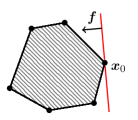
Figure 1: Linear program with 6 constraints that minimizes $b={\boldsymbol{f}}^{\intercal}{\boldsymbol{x}}$. All points on the red line have the same value $b$ for the objective function. The vertex $\boldsymbol{x}_{0}$ has the optimal value among all points in the feasible region.

The problem is called feasible if the polyehdron $\mathcal{P}$ is non-empty. Depending on the shape of the polyhedron $\mathcal{P}$ and optimization direction $\boldsymbol{f}$, the problem may either be bounded or unbounded. If $\mathcal{P}$ is bounded, the optimization problem is always bounded.

Although LP is known to have polynomial complexity Khachiyan (1980); Karmarkar (1984), the most widespread algorithm in use is simplex Dantzig (1990), which has exponential worst case scaling but performs quite well in practice Spielman and Teng (2001).

II.5 Machine-proving constraints

We frequently encounter the need to check whether a given constraint ${\boldsymbol{f}}^{\intercal}{\boldsymbol{x}}\geq b$ follows from a given set of inequalities $L\boldsymbol{x}\geq\boldsymbol{a}$. This can be decided by the LP (3). In this notation it is a trivial observation that the constraint ${\boldsymbol{f}}_{b}$ is valid if and only if the final objective function ${\boldsymbol{f}}^{\intercal}{\boldsymbol{x}}$ agrees with ${\boldsymbol{f}}_{b}$, i.e. ${\boldsymbol{f}}^{\intercal}{\boldsymbol{x}}\geq b$. The same condition applies for infinite objective values.

We now give a review of known elimination methods.

III Fourier-Motzkin elimination (FME)

Fourier-Motzkin elimination (FME) is perhaps the most straightforward approach for solving systems of linear inequalities. The basic procedure is to algebraically eliminate one variable after the other, as in Algorithm 1. It is comparable with Gaussian elimination known for systems of linear equalities. What is different from that case is that linear inequalities are not scalable by negative factors. Hence, after having selected one variable for elimination, the elimination step is carried out by partitioning the inequalities according to the sign of the coefficient for the active variable. Those inequalities with zero coefficient can be added unmodified to the result of the current step. Then, each pairing between inequalities with positive and negative sign is scaled and added up to eliminate the selected variable; after which the resulting inequality is appended to the result of the current step. For a detailed explanation including examples and additional mentions for applications see for example Williams (1986) or Huynh et al. (1990).

Algorithm 1 Fourier-Motzkin elimination to compute the projection $\pi_{d}(\mathcal{P})$ of an arbitrary polyhedron $\mathcal{P}=\{\boldsymbol{x}\in\mathbbm{R}^{d}+e:L\boldsymbol{x}\geq\boldsymbol{a}\}$.

1:function FME(${L}_{\boldsymbol{a}}$, $d$, $e$)

2:     if $e=0$ then

3:         return ${L}_{\boldsymbol{a}}$      

4:     $\mathrlap{j}\phantom{L^{+}}\leftarrow d+e$

5:     $\mathrlap{L^{0}}\phantom{L^{+}}\leftarrow\{({L}_{\boldsymbol{a}})_{i}:L_{ij}=0\}$

6:     $\mathrlap{L^{\pm}}\phantom{L^{+}}\leftarrow\{({L}_{\boldsymbol{a}})_{i}:L_{ij}\gtrless 0\}$

7:     $\mathrlap{L^{\prime}}\phantom{L^{+}}\leftarrow\{p_{j}\,{{\boldsymbol{q}}_{b}}+q_{j}\,{{\boldsymbol{p}}_{a}}:{{\boldsymbol{p}}_{a}}\in L^{+},{\boldsymbol{q}}_{b}\in L^{-}\}$

8:     return $\textsc{FME}(L^{0}\cup L^{\prime},\ d,\ e{-}1)$

 Basic form of FME without redundancy removal nor other improvements.

III.1 Redundancy elimination and improvements

The main problem which FME suffers from is the matter of redundant intermediate representations and output: Some of the considered combinations of positive and negative input inequalities can produce constraints that are redundant with respect to the resulting system. This leads to intermediate systems being larger than necessary to fully characterize the projection — which in turn can lead to even more redundant constraints in the following steps. Without strategies for redundancy removal the problem can quickly grow out of control in terms of both time and memory requirements. These redundancies can occur independently of the inherent complexity of the intermediate systems, i.e. even if the minimally required number of inequalities is small. Several methods have been suggested to accommodate for redundancies. A good overview is given by Imbert in Imbert (1993).

The choice of redundancy detection is usually a trade-off between cost and effectiveness and can make the difference between finishing the computation in a matter of seconds, hours, years, or not at all in feasible time. A rigorous elimination of all redundancies can be achieved by using linear programing (LP) to check one by one all inequalities of the resulting set. This is a rather expensive operation, but can be well worth the cost in our experience.

There are various additional ways to improve the performance of FME. Techniques for exploiting sparsity of the underlying linear system have been suggested by Simon et al. in Simon and King (2005). This paper also mentions the matter of elimination order and suggests to use the standard rule from Duffin (1974) to select at each step the variable which presumably delays the growth of intermediate systems most effectively: Assuming that for variable $i$ the number of rows with positive and negative coefficients is $E_{i}^{+}$ and $E_{i}^{-}$ respectively, the rule says to eliminate the variable which minimizes $E_{i}^{+}E_{i}^{-}-(E_{i}^{+}+E_{i}^{-})$, i.e. worst-case size of the next intermediate system.

In fact, we found this heuristic in combination with a full LP-based redundancy elimination at every step to be highly effective. It was with this strategy, that we could finally compute the full marginal characterizations of the $\mathcal{C}_{4}$ and $\mathcal{C}_{5}$ pairwise hidden ancestor models that had previously remained uncracked in earlier work. For more details, see Section XV.

III.2 Approximate solutions

Despite the improvements mentioned above many problems are intractable using FME. In this case FME can still be used to compute outer approximations of the projection polyhedron, if no exact solution is required. One way to do this is by dropping inequalities from the input problem. The choice which inequalities to remove can be guided by other insights, e.g. always keeping a certain known set of non-interior points outside the corresponding polyhedron, but could also be arbitrary. After removing sufficiently many constraints, FME can be performed efficiently on the smaller system.

There is a related, more sophisticated strategy, described in Simon and King (2005), that keeps the number of constraints below a certain threshold after each elimination step.

The result of such methods may in general be a rather crude outer approximation that can be improved upon by performing the procedure multiple times and combining the results. In any case, the resulting inequalities need not be facets of the actual solution. This fact can be mitigated by computing from each output inequality a set of facets such that the inequality becomes redundant. We describe a method to perform this calculation in Section VII.4.

III.3 Complexity

Consider eliminating a single variable from a system of $N$ inequalities. In the worst-case half of the inequalities have a positive coefficient for the elimination variable and the other half has a negative coefficient, i.e. $E_{i}^{+}=E_{i}^{-}=N/2$. In that situation the first elimination step results in a new system with $N^{\prime}=(N/2)^{2}$ inequalities. Hence, performing $e$ successive elimination steps can result in up to $4(N/4)^{2^{e}}$ inequalities – which can easily be seen to be true by inserting this expression in the above recursive formula. Although performing redundancy removal can mitigate this problem in many practical cases, there are problems for which the output size –and hence computation time– is inherently doubly exponential in the problem dimension Davenport and Heintz (1988); Monniaux (2010).

In information theoretic applications, the size of the input system is exponential in the number $k$ of random variables, i.e. $d+e=(2^{k}-1)$ and we have at least the elemental inequalities, which are $N=k+\binom{k}{2}2^{k-2}\sim k^{2}2^{k}$ in number. If projecting to a much lower-dimensional subspace, i.e. $d\ll e$, then on the order of $e\approx 2^{k}$ elimination steps are required. Thus, naively applying FME the worst-case time and space requirements roughly build up to a triple-exponential tower,

$$(k^{2}2^{k})^{2^{2^{k}}}\sim 2^{2^{2^{k}}}.$$

IV Extreme Point Method (EPM)

The Extreme Point Method (EPM) has been formulated in Lassez (1990) and is presented more accessibly in Huynh et al. (1992). It is based on a geometric perspective on the algebraic structure of the problem – viewing the set of possible combinations of the original constraints as a polytope of its own.

IV.1 The base algorithm

Recall that FME constructs new constraints as non-negative linear combinations of the original constraints such that the coefficients for the eliminated variables vanish. This can be formulated in terms of another problem. Let $\mathcal{P}=\{\boldsymbol{x}\in\mathbbm{R}^{d}+e:L\boldsymbol{x}\geq\boldsymbol{a}\}$ the original polyhedron where the constraint matrix has $r$ rows. The set of non-negative linear combinations of rows of $L$ that eliminates all variables with index $i>d$ is the pointed convex cone defined by

$$\mathcal{Q} =\Big{\{}\boldsymbol{q}\in\mathbbm{R}^{r}:\boldsymbol{q}\geq\boldsymbol{0},\ (\boldsymbol{q}^{\intercal}L)_{i}=0\ \forall i>d,\ \textstyle{\sum_{j}}q_{j}=1\Big{\}}$$

It is sufficient to consider normalized $\boldsymbol{q}$ here since constraints can be scaled using non-negative factors. Every $\boldsymbol{q}\in\mathcal{Q}_{0}$ corresponds to a face ${\boldsymbol{f}}^{\intercal}{\boldsymbol{x}}\geq b$ of the projection $\pi_{d}(\mathcal{P})\subset\mathbb{R}^{d}$ with $\boldsymbol{f}={\boldsymbol{q}}^{\intercal}L$ and $b={\boldsymbol{q}}^{\intercal}{\boldsymbol{a}}$. Furthermore, like any polyhedron, $\mathcal{Q}_{0}$ is the convex combination of its extreme rays. Hence, any face with $\boldsymbol{f}={\boldsymbol{q}}^{\intercal}L$ for non-extremal $\boldsymbol{q}=\sum\lambda_{i}\boldsymbol{q}_{i}$ is a non-negative sum $\boldsymbol{f}=\sum\lambda_{i}\boldsymbol{f}_{i}$ of faces $\boldsymbol{f}_{i}={\boldsymbol{q}_{i}}^{\intercal}L$ and therefore necessarily redundant. This means that the set of facets of $\pi_{d}(\mathcal{P})$ can be obtained from the extreme points of $\mathcal{Q}$. More precisely, the facets of $\pi_{d}(\mathcal{P})$ are in one-to-one correspondence to extreme points of the image $\mathcal{Q}^{\intercal}L$. In Lassez (1990) this problem is called a generalized linear program.

Observe that this perspective transforms the problem to a polytope and allows any vertex enumeration method to be applied to solve the projection problem. The transformed domain is bounded, independently of whether the original polyhedron is bounded or not. This is especially interesting in the light of some projection methods that do not work well for general unbounded polyhedra such as the convex hull method to be presented in V.

Note that the map $\boldsymbol{q}\rightarrow{\boldsymbol{q}}^{\intercal}L$ is in general not injective and hence many extreme points of $\mathcal{Q}$ may correspond to the same face ${\boldsymbol{f}}^{\intercal}{\boldsymbol{x}}\geq b$ and need not even be facets of $\pi_{d}(\mathcal{P})$. In other words, there may be many possible combinations of the original constraints to obtain any particular facet of the projection body. This can lead to extreme degrees of degeneracy and means that the amount of extreme points of $\mathcal{Q}$ may become impractically large to iterate over.

IV.2 Partial solutions

If a complete enumeration of all vertices of $\mathcal{Q}$ is infeasible the structure of EPM can be exploited to obtain approximate solutions. In fact, since every vertex or boundary point of $\mathcal{Q}$ corresponds to a face of the projection polyhedron $\pi_{d}(\mathcal{P})$, any subset of such points corresponds to an outer approximation of $\pi_{d}(\mathcal{P})$. Points on the hull of $\mathcal{Q}$ can be directly obtained by solving the LP

$$\begin{split}&\operatorname{arg\,min}\,\boldsymbol{q}\mapsto{\boldsymbol{p}}^{\intercal}{\boldsymbol{q}}\\ &\text{subject to }\boldsymbol{q}\in\mathcal{Q}\end{split}$$ (5)

while imposing arbitrary but fixed vectors $\boldsymbol{p}\in\mathbbm{R}^{r}$.

The objective vectors $\boldsymbol{p}$ can be sampled at random or guided by more physical insight. One particularly useful approach is to use known points $\boldsymbol{x}\in\mathbbm{R}^{d}\subset\mathbbm{R}^{d}+e$ on the boundary or exterior of the projection $\pi_{d}(\mathcal{P})$ in the output space and letting $\boldsymbol{p}=L\boldsymbol{x}$. Then the LP (5) finds a face ${\boldsymbol{f}}_{b}={\boldsymbol{q}}^{\intercal}{L}_{\boldsymbol{a}}$ of $\pi_{d}(\mathcal{P})$ which proves that $\boldsymbol{x}$ is not in the interior of $\pi_{d}(\mathcal{P})$, i.e. ${\boldsymbol{f}}^{\intercal}{\boldsymbol{x}}\leq b$.

Whenever the output is only a regular face and not a facet of $\pi_{d}(\mathcal{P})$, a corresponding set of facets can be derived using the strategy that will be discussed in Section VII.4. In other words, this method allows to convert an outer approximation specified as the convex hull of a set of points to an outer approximation in terms of facets. See Algorithm 13 for further reference.

While this last property can be particularly useful, we note that in our experiments, the partial EPM yielded only a small fraction of the facets that we could discover using other methods. This can be understood given the expected degeneracies that was already mentioned in the preceding subsection. Some facets $\boldsymbol{f}={\boldsymbol{q}}^{\intercal}L$ are in correspondence with many vertices $\boldsymbol{q}$ of $\mathcal{Q}$ and are therefore very likely to be encountered over and over. For other facets only one or a few combinations $\boldsymbol{q}\in\mathcal{Q}$ may exist. Considering a large possible total number of vertices of $\mathcal{Q}$ this makes them unlikely to ever be produced by the randomized EPM as presented here.

IV.3 Complexity

A complete solution using EPM depends on the problem of vertex enumeration which is known to be hard Khachiyan et al. (2008); Bremner (1998). Furthermore, as briefly mentioned above, the number of extreme points of the combination polytope $\mathcal{Q}$ can become impractically large as to prevent basic iteration even if no additional computation cost for construction and redundancy removal were needed. In fact, for general $d$-dimensional polyhedra with $v$ vertices McMullen’s Upper Bound Theorem McMullen (1970) together with the Dehn-Sommerville equations Sommerville (1927) gives a tight upper bound on the number of its facets $f$. By duality

$$v \leq\textstyle{\binom{f-d-s}{s}+\binom{f-s-1}{d-s-1}}=\mathcal{O}(f^{s}),$$

where $s=\lfloor d/2\rfloor$. However, problems in information theory exhibit more structure than general polyhedra and hence can be subjected to tighter bounds. Depending on the exact structure of the problem, one of the bounds in Elbassioni et al. (2006) is applicable. The best of these bounds that applies to $\mathcal{Q}$ arising from unconstrained Shannon cones $\mathcal{C}=\{\boldsymbol{x}:L\boldsymbol{x}\geq\boldsymbol{0}\}$ limits the number of vertices of $\mathcal{Q}$ to

$$v \leq 8^{d},$$

where $d+1=r$ is the number of rows of $L$. In a system with $n$ random variables, we have $r=n+\binom{n}{2}2^{n-2}$ elemental inequalities and thus the number of vertices of $\mathcal{Q^{\prime}}$ is bounded by an expression that is doubly exponential in $n$.

V Convex Hull Method (CHM)

The Convex Hull Method (CHM) uses a geometric approach to perform the subspace projection without going through the descriptions of any intermediate systems. The method was shortly mentioned in Taylor and Rajan (1988) and more thoroughly treated in Lassez and Lassez (1990) and Huynh et al. (1992). Since we came up with this algorithm independently and without knowledge of their work, our specification of the algorithm is slightly different from theirs and is listed in more mathematical –less imperative– notation. This may be useful as to provide an alternative reference on the problem.

The algorithm in the form discussed here is applicable when the output is a polytope. Pointed convex cones, such as Shannon cones, can be considered polytopes by adding limiting constraints in the unbounded direction. Detailed considerations about the application of this method to convex cones and general unbounded polyhedra can be found in Lassez and Lassez (1990).

V.1 Description of the algorithm

The algorithm works in two phases. The first phase finds an initial set of vertices of the projection $\pi_{d}(\mathcal{P})$ that spans its full subspace. The convex hull of a subset of vertices is an inner approximation. The goal of the second phase is to incrementally improve the current inner approximation to finally arrive at the full facetal description of $\pi_{d}(\mathcal{P})$.

Algorithm 2 Compute the facets of a projection polytope $\pi_{d}(\mathcal{P})$ where $\mathcal{P}=\{\boldsymbol{x}\in\mathbbm{R}^{d}+e:L\boldsymbol{x}\geq\boldsymbol{a}\}$.

1:function chm(${L}_{\boldsymbol{a}}$, $d$)

2:     $\mathcal{V}\leftarrow\textsc{basis\,simplex}({L}_{\boldsymbol{a}},\ d)$

3:     return $\textsc{expand}({L}_{\boldsymbol{a}},\ d,\ \mathcal{V})$

 

The initial step of the CHM algorithm is to find a simplex that serves as a fully dimensional inner approximation to the projection $\pi_{d}(\mathcal{P})\subset\mathbbm{R}^{d}$. It works by repeatedly solving the LP

$$\begin{split}&\operatorname{arg\,min}\,\boldsymbol{x}\mapsto{\boldsymbol{g}}^{\intercal}{\boldsymbol{x}}\\ &\text{subject to }L\boldsymbol{x}\geq\boldsymbol{a},\end{split}$$ (6)

for every basis direction $\boldsymbol{g}\in\mathbb{R}^{d}$ of the projection subspace in order to find points on the boundary of $\pi_{d}(\mathcal{P})$. The exact procedure is described by Algorithm 3. The recommended implementation replaces the LP (6) with a dedicated function find vertex to make sure that every point in the result is a vertex of $\pi_{d}(\mathcal{P})$.

Algorithm 3 Compute a fully dimensional simplex of vertices of the projection polytope $\pi_{d}(\mathcal{P})$ where $\mathcal{P}=\{\boldsymbol{x}\in\mathbbm{R}^{d}+e:L\boldsymbol{x}\geq\boldsymbol{a}\}$.

1:function basis simplex(${L}_{\boldsymbol{a}}$, $d$)

2:     $\boldsymbol{g}\leftarrow$ choose $\boldsymbol{g}\in\mathbb{R}^{d}$

3:     $\boldsymbol{x}_{0}\leftarrow\textsc{find\,vertex}({L}_{\boldsymbol{a}},\ d,\ \boldsymbol{g})$

4:     $\mathcal{B}\leftarrow\{\boldsymbol{x}_{0}\}$

5:     $\mathcal{N}\leftarrow\emptyset$

6:     for $i$ in $1\ldots d$  do

7:         $\boldsymbol{g}\leftarrow$ choose $\boldsymbol{g}\in\mathcal{N}^{\perp}\subset\mathbb{R}^{d}$

8:         $\boldsymbol{x}_{i}\leftarrow\textsc{find\,vertex}({L}_{\boldsymbol{a}},\ d,\ \boldsymbol{g})$

9:         if ${\boldsymbol{g}}^{\intercal}(\boldsymbol{x}_{i}-\boldsymbol{x}_{0})=0$ then

10:              $\boldsymbol{x}_{i}\leftarrow\textsc{find\,vertex}({L}_{\boldsymbol{a}},\ d,\ -\boldsymbol{g})$          

11:         if ${\boldsymbol{g}}^{\intercal}(\boldsymbol{x}_{i}-\boldsymbol{x}_{0})=0$ then

12:              $\mathcal{N}\leftarrow\mathcal{N}\cup\{\boldsymbol{g}\}$

13:         else

14:              $\mathcal{N}\leftarrow\mathcal{N}\cup\{\boldsymbol{x}_{i}-\boldsymbol{x}_{0}\}$

15:              $\mathcal{B}\leftarrow B\cup\{\boldsymbol{x}_{i}\}$               

16:     return $\mathcal{B}$

 

Algorithm 4 Find a vertex of $\pi_{d}(\mathcal{P})$ that minimizes the objective ${\boldsymbol{q}}^{\intercal}{\boldsymbol{x}}$

1:function find vertex(${L}_{\boldsymbol{a}}$, $d$, $\boldsymbol{q}$)

2:     $\boldsymbol{q}_{1}\ldots\boldsymbol{q}_{d}\leftarrow\text{ ONB of }\mathbb{R}^{d}\text{ with }\boldsymbol{q}_{1}=\boldsymbol{q}$

3:     for $i$ in $1\ldots d$ do

4:         $\boldsymbol{x}_{i}\leftarrow\operatorname{arg\,min}\,\boldsymbol{x}\mapsto{\boldsymbol{q}}^{\intercal}_{i}\boldsymbol{x}\$ s.t. $L\boldsymbol{x}\geq\boldsymbol{a}$

5:         $\boldsymbol{x}_{i}\leftarrow\operatorname{arg\,min}\,\boldsymbol{x}\mapsto{\boldsymbol{q}}^{\intercal}_{i}\boldsymbol{x}\$ s.t. ${\boldsymbol{q}}^{\intercal}_{j}\boldsymbol{x}={\boldsymbol{q}}^{\intercal}_{j}\boldsymbol{x}_{j}\,\forall j<i$      

6:     return $\pi_{d}(\boldsymbol{x}_{d})$

 Use this function in place of a simple minimization of ${\boldsymbol{q}}^{\intercal}{\boldsymbol{x}}$ subject to $L\boldsymbol{x}\geq\boldsymbol{a}$, where a true vertex is desired as the result. This function is not strictly required for the correctness of CHM (in neither of the two phases), but constitutes an important optimization by keeping the number of points on which the convex hull operation in the second phase is performed down to a minimum.

As far as dimensionality is concerned, any potential equality constraints are automatically detected during the initialization phase (null space is described by the contents $\mathcal{N}$). It is then sufficient to perform the second phase of the convex hull operation in the subspace in which $\pi_{d}(\mathcal{P})$ is fully dimensional.

This algorithm has a corollary use since it effectively computes the (affine) subspace in which the projection $\pi_{d}(\mathcal{P})$ is contained. In particular, this can be used to compute the rank of a face ${\boldsymbol{f}}^{\intercal}{\boldsymbol{x}}\geq b$ by performing the initialization step after augmenting the constraint list with ${\boldsymbol{f}}^{\intercal}{\boldsymbol{x}}=b$, see Algorithm 5.

Algorithm 5 Determine the rank of a face ${\boldsymbol{f}}^{\intercal}{\boldsymbol{x}}\geq b$ of $\pi_{d}(\mathcal{P})$. This is a corollary use of the initialization step of CHM.

1:function face rank(${L}_{\boldsymbol{a}}$, $d$, $\boldsymbol{f}$)

2:     $\mathcal{S}\leftarrow\textsc{basis\,simplex}({L}_{\boldsymbol{a}}\cup\{-{\boldsymbol{f}}_{b}\},\ d)$

3:     return $\lvert\mathcal{S}\rvert-1$

 

V.2 Incremental refinement

Figure 2: The facet construction phase of the Convex Hull Method. Start with a $d$-simplex of vertices and compute their convex hull. Check each element of the hull if it corresponds to a valid constraint of the system using a linear program. For each invalid constraint, the LP outputs an additional point that violates this constraint. Add all vertices and recompute the convex hull. Continue until all faces are valid constraints.

The second phase of CHM iteratively improves the current inner approximation. This is based on the fact that each facet of the convex hull of the currently known vertices is either a facet of $\pi_{d}(\mathcal{P})$ – or is violated by a vertex of $\pi_{d}(\mathcal{P})$. In the second case, the vertex is added to the list of known vertices and the step can be repeated until no facet of the convex hull is violated. The process is depicted in Figure 2. A rule of thumb is to add as many vertices as possible before starting the computation of the next hull. Known symmetries of the output polytope can be exploited by immediately taking into account all points in the orbit of a newly discovered point.

Algorithm 6 Second phase of the CHM algorithm to compute the facets of the projection polytope $\pi_{d}(\mathcal{P})$. Given a set of vertices $\mathcal{V}$, finds missing vertices of $\pi_{d}(\mathcal{P})$ until all are known.

1:function expand(${L}_{\boldsymbol{a}}$, $d$, $\mathcal{V}$)

2:     $\mathcal{U}\leftarrow\emptyset$

3:     $\mathcal{F}\leftarrow\textsc{convex\,hull}(\mathcal{V})$

4:     for ${\boldsymbol{f}}_{b}\in\mathcal{F}$ do

5:         $\boldsymbol{x}\leftarrow\operatorname{arg\,min}\,\boldsymbol{x}\mapsto{\boldsymbol{f}}^{\intercal}{\boldsymbol{x}}\$ s.t $\ L\boldsymbol{x}\geq\boldsymbol{a}$

6:         if ${\boldsymbol{f}}^{\intercal}{\boldsymbol{x}}<b$ then

7:              $\mathcal{U}\leftarrow\mathcal{U}\cup\{\textsc{find\,vertex}({L}_{\boldsymbol{a}},\ d,\ \boldsymbol{f})\}$               

8:     if $\mathcal{U}=\emptyset$ then

9:         return $\mathcal{F}$      

10:     return $\textsc{expand}({L}_{\boldsymbol{a}},\ d,\ \mathcal{V}\cup\mathcal{U})$

 

V.3 Complexity

Contrary to FME, the runtime of CHM does not depend on the size of intermediate projections. Further, while it is hard to cast useful runtime predictions in terms of the input parameters (dimension, size) of the problem, it can be specified relatively well in terms of the output size, i.e. the dimension and number of vertices of the output polytope. This characterizes CHM as output sensitive and makes it a promising algorithm for many projection problems that appear intractable with FME. In practice CHM only performs well if the dimension of the output space is sufficiently low and the number of vertices is small.

To make this more precise, assume that $\pi_{d}(\mathcal{P})$ is a $d$ dimensional polytope with $v$ vertices and $f$ facets. For $d>3$ the computation of the convex hull then takes time $\mathcal{O}(v^{\lfloor d/2\rfloor})$. Let’s imagine we have access to an online convex hull algorithm that spits out exactly one new facet of the convex hull $\operatorname{CH}(\mathcal{V})$ each time that we ask it to. Every one of these facet candidates needs to be checked using a single LP instance. It can either be a valid facet of $\pi_{d}(\mathcal{P})$ – or the result of the LP is a new point on the boundary, which can be converted to a vertex. This means that, in addition to the convex hull operation itself, only $(v+f)$ LPs need to be solved before we arrive at the final solution. The total work required is thus Chazelle (1993)

$$\mathcal{O}(v^{\lfloor d/2\rfloor})+(v+f)\cdot\mathrm{LP}.$$

Perceivably, the bottle neck of this algorithm is the computation of the convex hull in the output space.

The actual implementation used to obtain our results is based on a non-incremental convex hull solver – i.e. the hull is computed multiple times without incorporating the knowledge of previous computations. At every step each facet of the current inner approximation is checked using an LP. An invalid constraint will lead to the discovery of a new vertex. Therefore, at least one new vertex is added at each step as long as the description is incomplete. If only a single vertex is added at each step, the total work spent on convex hulls is:

$$\sum_{k=0}^{v}\mathcal{O}(k^{\lfloor d/2\rfloor}) \lesssim\mathcal{O}(v\cdot v^{\lfloor d/2\rfloor})$$

$$=\mathcal{O}(v^{\lfloor d/2\rfloor+1}).$$

It can easily be seen that this worst-case corresponds to stopping when the first invalid facet candidate vector is encountered at each step. In this case, the total number of LP instances is $(v+f)$, again. If the strategy is changed to allow testing more than one invalid facet candidate, the number of LP instances can be limited to be any desired value above $(v+f)$. Typically, testing all new candidates is the best strategy as it maximizes the probability to find as many new vertices as possible in each iteration and therefore minimizes the number of iterations, i.e. convex hull operations.

VI Equality Set Projection (ESP)

In a 2004 paper Jones et al. (2004), Jones et al. described an algorithm called Equality Set Projection (ESP). Similar to CHM, this output-sensitive method computes the projection of polytopes directly in the output space without going through intermediate representations. It is based on the underlying principle that the faces of a polytope form a connected graph by the subset relation. Two $n$-dimensional faces are called adjacent if they share an $(n{-}1)$-dimensional subface. The principle of ESP is to first find an arbitrary facet, and then compute its adjacencies. This computation can be understood as a rotation of the facet around the ridge, as displayed in Figure 3.

Mathematically, ESP relies on the insight that every face of a polytype can be uniquely identified with a so-called equality set, which is the set of all input inequalities that are satisfied with equality on all points of the given face. The ESP rotation operation to find adjacent facets and the discovery of an initial facet can be performed using linear algebra on submatrices corresponding to the rows in the equality set and require the solution of only very few linear programs.

An in-depth description of the mathematics required to implement ESP is beyond the scope of this paper. The interested reader is well advised to read the article Jones et al. (2004). Instead, we will present in the next section a related method that we came up with before we knew about the existence of ESP. It has the same geometric interpretation and is easier to implement, but offers less potential optimizations. One interesting property of ESP compared to our method is that it can skip the recursion to compute lower dimensional faces of the projection polytope in the non-degenerate case.

Another noteworthy side-effect of the identification with equality sets is that faces of the projection polytope can be labeled with a tuple of numbers. This allows a constant time lookup operation for already computed faces (using a hash-table). This is important for avoiding recomputation of subfaces with multiple parents. Our AFI implementation in contrast depends on a linear number of matrix multiplications to achieve the same.

VII A new method: Adjacent facet iteration

We now present our own method, which is very similar to Equality Set Projection, but uses a different set of primitives that appears easier to implement. Contrary to ESP, we always require a recursive solution in the lower dimensional subspace.

VII.1 The base algorithm

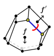
Figure 3: Adjacent facet iteration: First compute the subfacets of a given facet $\boldsymbol{f}$ and then use every subfacet to obtain an adjacent facet $\boldsymbol{f}^{\prime}$.

The core idea behind AFI is to traverse the face graph of the output polytope by moving along adjacencies (see Figure 3). More precisely, two facets of a $d$-dimensional polytope are said to be adjacent if their intersection is a $(d{-}2)$-dimensional face (ridge). With this notion of adjacency the facets of a polytope form a connected graph by duality of Balinski’s theorem Balinski (1961). Knowing a facet and one of its ridges the adjacent facet can be obtained using an LP-based rotation operation. Hence, presuming the knowledge of an arbitrary initial facet of a $d$-dimensional polytope all further facets can be iteratively determined by computing the ridges of every encountered facet, i.e. solving the projection problem for several $(d{-}1)$-dimensional polytopes. The lower dimensional projection algorithm can be chosen at will. For example, all AFI-based computations mentioned in this article were carried out by a $k$-level AFI recursion on top of CHM, i.e.

$$\begin{split}\operatorname{AFI_{k}}&:=\textsc{afi}\left[\Pi=\operatorname{AFI_{k-1}}\right],\\ \operatorname{AFI_{0}}&:=\textsc{chm}.\end{split}$$ (7)

Choosing $k$ is not only a matter of performance but also allows to control the amount of information that is recovered about the polytope. For example, $\operatorname{AFI_{1}}$ lists all vertices, ridges and facets; $\operatorname{AFI_{d}}$ outputs the entire face skeleton.

Algorithm 7 Compute the facets of $\pi_{d}(\mathcal{P})$ using AFI.

1:$\Pi$ computes $\pi_{d-1}(\mathcal{P}^{\prime})$

2:function afi$\left[\Pi\right]$(${L}_{\boldsymbol{a}}$, $d$)

3:     $\mathcal{R}\leftarrow\emptyset$

4:     $\mathcal{Q}\leftarrow\{\textsc{getfacet}({L}_{\boldsymbol{a}},\ d)\}$ $\triangleright$ uninspected facets

5:     while $\mathcal{Q}\neq\emptyset$ do

6:         ${\boldsymbol{f}}_{b}\leftarrow$ pop from $\mathcal{Q}$

7:         if ${\boldsymbol{f}}_{b}\not\in\mathcal{R}$ then

8:              $\mathcal{R}\leftarrow\mathcal{R}\cup\{{\boldsymbol{f}}_{b}\}$

9:              for $\boldsymbol{s}_{c}\in\Pi({L}_{\boldsymbol{a}}\cup\{-{\boldsymbol{f}}_{b}\},\ d)$ do

10:                  $\boldsymbol{f}^{\prime}_{b^{\prime}}\ \boldsymbol{s}^{\prime}_{c^{\prime}}\leftarrow\textsc{rotate}({L}_{\boldsymbol{a}},\ {-}{\boldsymbol{f}}_{b},\ \boldsymbol{s}_{c})$

11:                  $\mathcal{Q}\leftarrow\mathcal{Q}\cup\{\boldsymbol{f}^{\prime}_{b^{\prime}}\}$                             

12:     return $\mathcal{R}$

 The algorithm as listed here is kept simple for clarity and has no protection from calculating the projection of the same face multiple times. It is advisable to add a cache to AFI implementations that prevents this from happening.

Initial facet

Figure 4: Obtain an initial facet by successively fitting an arbitrary face onto the polyhedron – at each step increasing the face rank by one.

AFI requires a facet of the output polyhedron as initializer. In cases where no facet is known a priori, one can be obtained by successively increasing the rank of an arbitrary face. Geometrically, this can be pictured as rotating the face onto the polyhedron as shown in Figure 4. The algorithm is described in Algorithm 8.

The outcome of this procedure depends on a several arbitrary choices and can for appropriate values have any facet as a result. Thus, it is suggestive to employ this method repeatedly with the expectation that after enough iterations every facet will eventually be discovered. In practice, it turns out that this strategy typically recovers only a small number of facets even after long searches – similar to the randomized EPM discussed in Section IV.2.

Algorithm 8 Compute an (arbitrary) facet of $\pi_{d}(\mathcal{P})$.

1:function getfacet(${L}_{\boldsymbol{a}}$, $d$)

2:     $\boldsymbol{p}\leftarrow$ choose $\boldsymbol{p}\in\mathbbm{R}^{m}$

3:     $\boldsymbol{q}\leftarrow\operatorname{arg\,min}\,\boldsymbol{q}\mapsto{\boldsymbol{p}}^{\intercal}{\boldsymbol{q}}\$ s.t. $\boldsymbol{q}\geq\boldsymbol{0},\ \textstyle{\sum_{j}}q_{j}=1$,

4:     $\boldsymbol{q}\leftarrow\operatorname{arg\,min}\,\boldsymbol{q}\mapsto{\boldsymbol{p}}^{\intercal}{\boldsymbol{q}}\$ s.t. $({\boldsymbol{q}}^{\intercal}L)_{i}=0\ \forall i>d$

5:     return $\textsc{tofacet}({L}_{\boldsymbol{a}},\ d,\ {\boldsymbol{q}}^{\intercal}{L}_{\boldsymbol{a}})$

 For production use you should additionally take care to handle the case ${\boldsymbol{q}}^{\intercal}L=0$.

Algorithm 9 Turn a valid constraint on $\pi_{d}(\mathcal{P})$ into a facet.

1:function tofacet(${L}_{\boldsymbol{a}}$, $d$, $\boldsymbol{f}_{b}$)

2:     $\mathcal{P}\leftarrow\textsc{basis\,simplex}({L}_{\boldsymbol{a}},\ d)$

3:     $\mathcal{F}\leftarrow\textsc{basis\,simplex}({L}_{\boldsymbol{a}}\cup\{-{\boldsymbol{f}}_{b}\},\ d)$

4:     if ${\lvert\mathcal{F}\rvert}=\lvert\mathcal{P}\rvert-1$ then

5:         return $\boldsymbol{f}_{b}$      

6:     $\boldsymbol{s}\leftarrow$ choose $\boldsymbol{s}\in\langle\mathcal{P}-\mathcal{P}_{0}\rangle\cap\langle\mathcal{F}-\mathcal{F}_{0},\boldsymbol{f}\rangle^{\perp},\ \boldsymbol{s}\neq 0$

7:     $\boldsymbol{x}\leftarrow\operatorname{arg\,min}\,\boldsymbol{x}\mapsto{\boldsymbol{s}}^{\intercal}{\boldsymbol{x}}\$ s.t. $L\boldsymbol{x}\geq\boldsymbol{a}$

8:     $c\leftarrow{\boldsymbol{s}}^{\intercal}{\mathcal{F}_{0}}$

9:     if ${\boldsymbol{s}}^{\intercal}{\boldsymbol{x}}\geq c$ then

10:         $\boldsymbol{s}_{c}\leftarrow-\boldsymbol{s}_{c}$      

11:     $\boldsymbol{f}_{b},\ \boldsymbol{s}_{c}\leftarrow\textsc{rotate}({L}_{\boldsymbol{a}},\ {-}\boldsymbol{f}_{b},\ {-}\boldsymbol{s}_{c})$

12:     return $\textsc{tofacet}({L}_{\boldsymbol{a}},\ d,\ \boldsymbol{f}_{b})$

 

Computing adjacencies

Figure 5: Computation of the adjacent facet $\boldsymbol{f}^{\prime}$ from the facet $\boldsymbol{f}$ and a subface $\boldsymbol{s}$. Start with $\boldsymbol{g}_{0}{=}{-}\boldsymbol{f}$, $\boldsymbol{s}_{0}{=}\boldsymbol{s}$. Iteratively obtain $\boldsymbol{x}_{i}$ from the minimization of ${\boldsymbol{g}_{i}}^{\intercal}{\boldsymbol{x}}$ and then proceed by constructing new $\boldsymbol{s}_{i+1}\perp\boldsymbol{g}_{i+1}$ such that $\boldsymbol{g}_{i+1}$ is orthogonal to both $\boldsymbol{x}_{i}$ and $\mathcal{K}$.

At the heart of AFI is an LP-based rotation operation that computes the adjacent facet $\boldsymbol{f}^{\prime}_{b^{\prime}}$ given an initial facet $\boldsymbol{f}_{b}$ and one of its subfacets $\boldsymbol{s}_{c}$. The procedure is based on the fact that any $(d{-}2)$-face of an $d$-dimensional convex polyhedron $\mathcal{P}$ is the intersection of precisely two adjacent facets of $\mathcal{P}$ Grünbaum (1967). The normal vector $\boldsymbol{f}^{\prime}$ must be orthogonal to the $(d{-}2)$-dimensional (affine) subspace in which the subface denoted by $\boldsymbol{s}_{c}$ is fully dimensional. This means $\boldsymbol{f}^{\prime}$ must lie in the 2D plane spanned by the vectors $\boldsymbol{s}$ and $\boldsymbol{f}$. Hence, the problem is effectively to find the correct rotation angle of $\boldsymbol{f}^{\prime}$. Our strategy is to successively obtain candidates for $\boldsymbol{f}^{\prime}_{b^{\prime}}$ that increase the rotation angle in only one sense and converge toward the real value. This is achieved by searching for $\boldsymbol{x}_{i}$ that violates the current candidate and then constructing a new candidate that contains $\boldsymbol{x}_{i}$. Figure 5 shows this process in the $\langle\boldsymbol{f},\boldsymbol{s}\rangle$ plane. The method is like a partial CHM in 2D where we only care about the outermost face instead of computing the whole convex hull. With the precise specification of rotation operation as listed in Algorithm 10 the adjacent facet vector is obtained as $\boldsymbol{f}^{\prime}_{b^{\prime}}=\textsc{rotate}({L}_{\boldsymbol{a}},\ {-}{\boldsymbol{f}}_{b},\ \boldsymbol{s}_{c})$. In a sense rotate represents a very local operation in the output space. This is indicated by the fact that it depends only on the input constraints as well as the face and subface vectors, but e.g. not on the global output space $\mathbbm{R}^{d}$ directly.

Algorithm 10 Rotate a face of $\pi_{d}(\mathcal{P})$ around one of its subfaces.

1:candidates $\boldsymbol{g}_{b}$ for the rotated face and a subface $\boldsymbol{s}_{c}$ where $\boldsymbol{s}\perp\boldsymbol{g}$.

2:function rotate(${L}_{\boldsymbol{a}}$, $\boldsymbol{g}_{b}$, $\boldsymbol{s}_{c}$)

3:     $\boldsymbol{x}\leftarrow\operatorname{arg\,min}\,\boldsymbol{x}\mapsto{\boldsymbol{g}}^{\intercal}{\boldsymbol{x}}\$ s.t. $L\boldsymbol{x}\geq\boldsymbol{a}$

4:     if ${\boldsymbol{g}}^{\intercal}{\boldsymbol{x}}\geq b$ then

5:         return $\boldsymbol{g}_{b}$, $\boldsymbol{s}_{c}$      

6:     $\boldsymbol{g}_{b}\leftarrow\boldsymbol{g}_{b}/\lVert\boldsymbol{g}\rVert$, $\gamma\leftarrow{\boldsymbol{g}}^{\intercal}{\boldsymbol{x}}-b$

7:     $\boldsymbol{s}_{c}\leftarrow\boldsymbol{s}_{b}/\lVert\boldsymbol{s}\rVert$, $\sigma\leftarrow{\boldsymbol{s}}^{\intercal}{\boldsymbol{x}}-c$

8:     return $\textsc{rotate}({L}_{\boldsymbol{a}},\ \sigma\boldsymbol{g}_{b}{-}\gamma\boldsymbol{s}_{c},\ \gamma\boldsymbol{g}_{b}{+}\sigma\boldsymbol{s}_{c})$

 Given an invalid constraint $\boldsymbol{g}_{b}$ the result is a face that touches the polytope in the $\langle\boldsymbol{g},\boldsymbol{s}\rangle$ plane. This property is exploited by the tofacet routine to successively increase the face rank.

The update rules for $\boldsymbol{g}_{b}$ and $\boldsymbol{s}_{c}$ in rotate can be derived using the following simple argument. Assume normalized constraints $\boldsymbol{g}_{b}$ and $\boldsymbol{s}_{c}$ with $\boldsymbol{g}\perp\boldsymbol{s}$. At each step, we search for $\boldsymbol{g}^{\prime}$ in the 2D plane spanned by $\boldsymbol{g}$ and $\boldsymbol{s}$, i.e. $\boldsymbol{g}^{\prime}=\alpha\boldsymbol{g}+\beta\boldsymbol{s}$. Let now $\boldsymbol{y}=b\boldsymbol{g}+c\boldsymbol{s}$ at the intersection of $\boldsymbol{g}_{b}$ and $\boldsymbol{s}_{c}$. Then, since $\boldsymbol{g}^{\prime}_{b^{\prime}}$ should contain $\boldsymbol{x}$ and $\boldsymbol{y}$, we must have for $\boldsymbol{z}=\boldsymbol{x}-\boldsymbol{y}$

$$0 ={\boldsymbol{z}}^{\intercal}{\boldsymbol{g}^{\prime}}=\alpha{\boldsymbol{z}}^{\intercal}{\boldsymbol{g}}+\beta{\boldsymbol{z}}^{\intercal}{\boldsymbol{s}}=\alpha\gamma+\beta\sigma,$$

with $\gamma={\boldsymbol{g}}^{\intercal}{\boldsymbol{x}}-b$ and $\sigma={\boldsymbol{s}}^{\intercal}{\boldsymbol{x}}-c$. To enforce a rotation toward $\boldsymbol{s}$, demand

$$0 \stackrel{{\scriptstyle!}}{{<}}{\boldsymbol{s}}^{\intercal}{\boldsymbol{g}^{\prime}}=\alpha\underbrace{{\boldsymbol{s}}^{\intercal}{\boldsymbol{g}}}_{=0}+\beta\underbrace{{\boldsymbol{s}}^{\intercal}{\boldsymbol{s}}\vphantom{\boldsymbol{g}}}_{=1}=\beta.$$

Furthermore, we know $\gamma={\boldsymbol{g}}^{\intercal}{\boldsymbol{x}}-b<0$ due to the break condition in line 4 of Algorithm 10. Therefore, the canonical choice for $\boldsymbol{g}^{\prime}$ is

$$\boldsymbol{g}^{\prime} =\sigma\boldsymbol{g}-\gamma\boldsymbol{s}.$$

The invariant $\boldsymbol{s}^{\prime}\perp\boldsymbol{g}^{\prime}$ is retained by using the projection of $\boldsymbol{z}$ as the new $\boldsymbol{s}^{\prime}$:

$$\boldsymbol{s}^{\prime} =\pi_{\langle\boldsymbol{s},\boldsymbol{g}\rangle}(\boldsymbol{z})=\left({\boldsymbol{s}{\boldsymbol{s}}^{\intercal}}+{\boldsymbol{g}{\boldsymbol{g}}^{\intercal}}\right)\boldsymbol{z}=\sigma\boldsymbol{s}+\gamma\boldsymbol{g}.$$

This also ensures a monotonous rotation sense. The inhomogeneities are obtained using corresponding linear combinations

$$b^{\prime} ={\boldsymbol{y}}^{\intercal}{\boldsymbol{g}}^{\prime}=\sigma b-\gamma c,$$

$$c^{\prime} ={\boldsymbol{y}}^{\intercal}{\boldsymbol{s}}^{\prime}=\gamma b+\sigma c.$$

VII.2 Exploiting symmetries

If the symmetry group $G$ of the output polytope is known it is sufficient to compute the adjacencies of only one representative $\boldsymbol{f}$ of every orbit $G\boldsymbol{f}$ since

$$\boldsymbol{f}^{\prime}(g\boldsymbol{f},g\boldsymbol{s})=g\boldsymbol{f}^{\prime}(\boldsymbol{f},\boldsymbol{s})$$

for every $g\in G$. This can be implemented by changing line 8 in Algorithm 7 to

$$\mathcal{R}\leftarrow\mathcal{R}\cup G\boldsymbol{f}.$$

This modification can speed up AFI by the average orbit size $\lvert G\boldsymbol{f}\rvert$.

VII.3 Randomized facet discovery (RFD)

When increasing the output dimension of the projection problem an AFI-based complete computation quickly becomes infeasible. However, a randomized variant of AFI can be highly effective for computing partial descriptions. The randomized facet discovery $\operatorname{RFD_{k,n}}$ recursively computes partial projections. It is defined similar to $\operatorname{AFI_{k}}$:

$$\operatorname{RFD_{k,n}}(\ldots) :=\textsc{afi}(\ldots,\operatorname{RFD_{k-1,n}}),$$

with the difference that CHM is carried out only $$n$$ times in total, i.e.

$$\operatorname{RFD_{0,n}}(\ldots) :=\textsc{chm}(\ldots)\quad\text{and decrease}\quad n\rightarrow n-1,$$

$$\operatorname{RFD_{0,0}}(\ldots) :=\emptyset.$$

Alternatively, carry out CHM $n$ times within every $\operatorname{RFD_{1,n}}$ call.

To improve the exhaustiveness of the RFD output, the routine can be invoked multiple times while preserving the knowledge about recovered polyhedral substructure. This means populating the queue $\mathcal{Q}$ on line 4 of Algorithm 7 with the known facets of the current polytope and selecting in line 6 the facet with the least known substructure.

The effectiveness of RFD is based on the observation that AFI usually recovers the full projection after only a few steps but takes longer to finish in order to make sure that no further facets are missing. In other words, to obtain the full solution it is sufficient to compute the adjacencies of a small subset of the facets. This can be understood as the result of a high connectivity among the facets: every facet is adjacent to at least $d$ other facets.

VII.4 Refining outer approximations (ROA)

We have seen that randomized variants of FME and EPM can provide outer approximations that can in general contain non-facetal elements, see Section III.2 and Section IV.2, respectively. With the tofacet routine (Algorithm 9) any given face can be transformed into a facet which contains the face as a subset. However, the result –being a single constraint– can not imply the input constraint (unless the input was a facet and is therefore returned unchanged) and even after mapping all faces of the outer approximation individually to facets this method can provide no guarantee that the result is a strictly tighter approximation. To remedy this issue we can construct a modified procedure tofacets that returns a set of facets that provide a sufficient replacement for the input constraint, see Algorithm 11.

This procedure has another remarkable use case: the point 2 facet routine returns facets which document that a given point is not in the interior of $\pi_{d}(\mathcal{P})$. This allows to turn an outer approximation in vertex representation into a (generally non-equivalent) outer approximation in half-space representation, see Algorithm 13, facilitated using the LP (5) from Section IV.2.

Algorithm 11 Convert an arbitrary face of $\pi_{d}(\mathcal{P})$ to a set of implying facets.

1:$R_{\boldsymbol{c}}$ set of known facets (can be initially empty)

2:function tofacets(${L}_{\boldsymbol{a}}$, $d$, ${\boldsymbol{f}}_{b}$, $R_{\boldsymbol{c}}$)

3:     $\boldsymbol{x}\leftarrow\operatorname{arg\,min}\,\boldsymbol{x}\mapsto{\boldsymbol{f}}^{\intercal}{\boldsymbol{x}}\$ s.t. $R\boldsymbol{x}\geq\boldsymbol{c}$

4:     if ${\boldsymbol{f}}^{\intercal}{\boldsymbol{x}}\geq b$ then

5:         return $R_{\boldsymbol{c}}$      

6:     $\boldsymbol{g}_{c}\leftarrow\textsc{tofacet}_{2}({L}_{\boldsymbol{a}},\ d,\ {\boldsymbol{f}}_{b},\ \boldsymbol{x})$

7:     return $\textsc{tofacets}({L}_{\boldsymbol{a}},\ d,\ {\boldsymbol{f}}_{b},\ R_{\boldsymbol{c}}\cup\{\boldsymbol{g}_{c}\})$

 

Algorithm 12 Convert a valid constraint on $\pi_{d}(\mathcal{P})$ into a facet using a non-interior control point.

1:function tofacet₂($L$, $d$, ${\boldsymbol{f}}_{b}$, $\boldsymbol{y}$)

2:     $\mathcal{P}\leftarrow\textsc{basis\,simplex}({L}_{\boldsymbol{a}},\ d)$

3:     $\mathcal{F}\leftarrow\textsc{basis\,simplex}({L}_{\boldsymbol{a}}\cup\{-{\boldsymbol{f}}_{b}\},\ d)$

4:     if ${\lvert\mathcal{F}\rvert}=\lvert\mathcal{P}\rvert-1$ then

5:         return $\boldsymbol{f}_{b}$      

6:     $\boldsymbol{s}\leftarrow$ choose $\boldsymbol{s}\in\langle\mathcal{P}-\mathcal{P}_{0}\rangle\cap\langle\mathcal{F}-\mathcal{F}_{0},\boldsymbol{f}\rangle^{\perp},\ \boldsymbol{s}\neq 0$

7:     $\boldsymbol{x}\leftarrow\operatorname{arg\,min}\,\boldsymbol{x}\mapsto{\boldsymbol{s}}^{\intercal}{\boldsymbol{x}}\$ s.t. $L\boldsymbol{x}\geq\boldsymbol{a}$

8:     $c\leftarrow{\boldsymbol{s}}^{\intercal}{\mathcal{F}_{0}}$

9:     if ${\boldsymbol{s}}^{\intercal}{\boldsymbol{x}}\geq c$ then

10:         $\boldsymbol{s}_{c}\leftarrow-\boldsymbol{s}_{c}$      

11:     $\boldsymbol{f}_{b},\ \boldsymbol{s}_{c}\leftarrow\textsc{rotate}({L}_{\boldsymbol{a}},\ -\boldsymbol{f}_{b},\ -\boldsymbol{s}_{c})$

12:     if ${\boldsymbol{g}}^{\intercal}{\boldsymbol{y}}>c$ then

13:         $\boldsymbol{f}_{b},\ \boldsymbol{s}_{c}\leftarrow\textsc{rotate}({L}_{\boldsymbol{a}},\ -\boldsymbol{f}_{b},\ \boldsymbol{s}_{c})$      

14:     return $\textsc{tofacet}_{2}({L}_{\boldsymbol{a}},\ d,\ \boldsymbol{f}_{b},\ \boldsymbol{y})$

 The resulting facet $\boldsymbol{f}_{c}$ proves that $\boldsymbol{y}$ is not an interior point of the projection polytope, i.e. ${\boldsymbol{f}}^{\intercal}{\boldsymbol{y}}\leq c$. The only difference from the regular tofacet procedure are the lines 12-14.

Algorithm 13 Turn an non-interior point into a set of facet, each of which proves that the point is non-interior.

1:function point 2 facet(${L}_{\boldsymbol{a}}$, $d$, $\boldsymbol{y}$)

2:     $\boldsymbol{q}\leftarrow\operatorname{arg\,min}\,\boldsymbol{q}\mapsto{\boldsymbol{q}}^{\intercal}L\boldsymbol{y}$ s.t. $\boldsymbol{q}\geq\boldsymbol{0},\ \textstyle{\sum_{j}}q_{j}=1,$

3:     $\boldsymbol{q}\leftarrow\operatorname{arg\,min}\,\boldsymbol{q}\mapsto{\boldsymbol{q}}^{\intercal}L\boldsymbol{y}$ s.t. $({\boldsymbol{q}}^{\intercal}L)_{i}=0\ \forall i>d$

4:     return $\textsc{tofacets}({L}_{\boldsymbol{a}},\ d,\ {\boldsymbol{q}}^{\intercal}{L}_{\boldsymbol{a}},\ \emptyset)$

 The routine can alternatively be implemented using directly the $\textsc{tofacet}_{2}$ primitive.

VII.5 Relation to other algorithms

The fully recursive $\operatorname{AFI_{d}}$ method uses the same geometric traversal strategy that is also used for the vertex enumeration method described by McRae and Davidson McRae and Davidson (1973). By duality, their method can be viewed as a convex hull algorithm. However, the algorithm differs from AFI in that it was not conceived as a projection algorithm and is therefore based on the assumption that the full half-space representation (or vertex representation in the case of convex hull) of the investigated polytope is already available to begin with. Hence, their rotation primitive is based on an algebraic approach which is not available for the projection problem.

In general, one class of convex hull algorithms is based on a pivoting operation that can be understood as a rotation around a ridge just as the one used in AFI, see e.g. Chand and Kapur (1970); Avis et al. (1997). In this sense, AFI can be comprehended as an online variant of convex hull that operates without knowing the full list of vertices in advance, but rather determines them as needed using LPs. Note that this represents an inversion of control when compared to online convex hull algorithms in the usual sense. These algorithms are operated in push-mode, i.e. vertices are fed to the algorithm from an outside operator (e.g. CHM) when they become available and the algorithm is expected to update its half-space representation after each transaction. In contrast, AFI operates in pull-mode, i.e. fetches vertices with specified properties as they are needed to compute a new facet.

VIII Comparison of algorithms

This section contains a short summary of the discussed algorithms and their strengths and weaknesses.

VIII.1 Fourier-Motzkin elimination

FME is an algebraic variable elimination by appropriately combining input inequalities. It works arbitrary polyhedra without further preparations, and is easy to understand and implement. FME can outperform other methods dramatically, in particular when the number of input inequalities is small and only a small number of variables have to be eliminated from the input problem. Despite its untracktable worst-case scaling, FME with redundancy elimination can therefore be a valueable tool. For many practical problems, however, FME falls victim to the combinatorial explosion. In such cases, consider applying a randomized FME as a first step to obtain outer approximations which can then be improved upon with other methods.

VIII.2 Extreme Point Method

This method works by searching for combinations of input inequalities that sum up to eliminate all but the output coordinates. While this is an insightful take on the problem, we found it impractical for our use-cases due to the degeneracy of the combination polytope with respect to the projection polyhedron. One interesting aspect of the algorithm is its use to search for random faces of the projection.

VIII.3 Convex Hull Method

CHM is a geometric method to compute the projection of polytopes. It works directly in the output space without going through intermediate systems like FME. Also contrary to FME, is output-sensitive and particularly efficient when the dimension of the output space is low. While performing CHM, you also acquire all vertices of the projection polytope.

VIII.4 Equality Set Projection

Like CHM, the ESP algorithm is an output-sensitive method suited to compute the projection of polytopes. In non-degenerate cases, ESP can be efficiently performed without having to solve the projection problem recursively for lower-dimensional faces. For such cases, ESP can be used even if there is a large number of vertices that would make CHM unpractical.

VIII.5 Adjacent Facet Iteration

AFI is a geometric approach that walks along the face lattice similar to ESP. Compared to ESP, it takes a cruder approach to compute adjacencies, relying entirely on LP based primitives. By our measure, this also makes the method easier to understand and implement. However, it also falls short on potential optimizations. It always requires recursion and can output the entire face skeleton of a polytope. Advantages of the AFI primitives are their corollary uses, e.g. to compute facets from known faces or non-interior points of the projection polytope, as well as the potential for application in randomized contexts.

Part II Quantum Nonlocality

IX Bell inequalities and marginal problems

We start describing the simplest non-trivial marginal problem. Consider you have three dichotomic random variables $X_{1},X_{2},X_{3}$ with $X_{i}\in\{\pm 1\}$ but can only sample two of them at a given time. Further, suppose that you observe perfect correlations between $X_{1}$ and $X_{2}$ and between $X_{1}$ and $X_{3}$, that is, $\langle X_{1}X_{2}\rangle=\langle X_{1}X_{3}\rangle=1$. Intuitively, since correlations are transitive, we would expect that in such a case the variables $X_{2}$ and $X_{3}$ should also be perfectly correlated, that is $\langle X_{2}X_{3}\rangle=1$. However, suppose we observe perfect anti-correlations $\langle X_{2}X_{3}\rangle=-1$. What does our intuition tell about such correlations?

Underlying the intuitive description of this simple experiment is the idea that there is a well defined (normalized and positive) joint probability distribution $p(x_{1},x_{2},x_{3})$ — even if empirically we can only sample two variables at a time, that is, we only have access to $p(x_{i},x_{j})$. As it turns out, the existence of a joint distribution $p(x_{1},x_{2},x_{3})$ implies strict constraints on the possible marginal distributions that can be obtained from it. In particular, it follows that

$$\langle X_{1}X_{2}\rangle+\langle X_{1}X_{3}\rangle\leq 1+\langle X_{2}X_{3}\rangle,$$ (8)

an inequality that is violated if

$$\langle X_{1}X_{2}\rangle=\langle X_{1}X_{3}\rangle=-\langle X_{2}X_{3}\rangle=1,$$ (9)

thus showing that such correlations cannot arise from an underlying joint distribution among the three variables.

An alternative description for the existence of a joint distribution among all the variables is given by

$$p(x_{i},x_{j})=\sum_{\lambda}p(\lambda)\,p(x_{i}\ooalign{$\phantom{{},{}}$\cr$|$}\lambda)\,p(x_{j}\ooalign{$\phantom{{},{}}$\cr$|$}\lambda),$$ (10)

that is, there is an underlying process, described by the unobserved (hidden) variable $\lambda$ that specifies the values of all variables $x_{i}$ independently of which variables we decide to sample at a given round of the experiment. What this shows is that correlations (9) cannot arise from such a process and can only be generate if $\lambda$ is correlated with our choices of which variables to sample at given run.

Bell’s theorem concerns a scenario very similar to this one. A Bell experiment involves two distant (ideally space-like separated) parties, Alice and Bob, that upon receiving physical systems can measure them using different observables. We denote the measurement choices and measurement outcomes of Alice and Bob by random variables $X$ and $Y$ and $A$ and $B$, respectively. A classical description of such experiment, imposes that the observable distribution $p(a,b\ooalign{$\phantom{{},{}}$\cr$|$}x,y)$ can be decomposed as

$$p(a,b\ooalign{$\phantom{{},{}}$\cr$|$}x,y)= \sum_{\lambda}p(a,b,\lambda\ooalign{$\phantom{{},{}}$\cr$|$}x,y)$$ (15)

$$= \sum_{\lambda}p(a,b\ooalign{$\phantom{{},{}}$\cr$|$}x,y,\lambda)\,p(\lambda\ooalign{$\phantom{{},{}}$\cr$|$}x,y)$$ (20)

$$= \sum_{\lambda}p(a\ooalign{$\phantom{{},{}}$\cr$|$}x,\lambda)\,p(b\ooalign{$\phantom{{},{}}$\cr$|$}y,\lambda)\,p(\lambda),$$ (25)

where the variable $\lambda$ represents the source of particles and any other local mechanisms in Alice and Bob laboratories that might affect their measurement outcomes. In (15) we have imposed the conditions $p(\lambda\ooalign{$\phantom{{},{}}$\cr$|$}x,y)=p(\lambda)$, $p(a\ooalign{$\phantom{{},{}}$\cr$|$}x,y,b,\lambda)=p(a\ooalign{$\phantom{{},{}}$\cr$|$}x,\lambda)$ and $p(b\ooalign{$\phantom{{},{}}$\cr$|$}x,y,a,\lambda)=p(b\ooalign{$\phantom{{},{}}$\cr$|$}y,\lambda)$. The first condition refers to measurement independence (or “free-will”) stating that the choice of which property of the physical system the observers decide to measure is made independently of how the system has been prepared. The second conditions related to local causality, that is, the probability of the measurement outcome $A$ is fully determined by events in its causal past, in that case the variables $X$ and $\lambda$ (and similarly to the measurement outcome $B$).

This classical description in terms of local hidden variable (LHV) model is equivalent to the existence of a joint distribution of measurement outcomes all possible measurements Fine (1982), that is, $p(a_{1},\dots,a_{\lvert x\rvert},b_{1},\dots,b_{\lvert y\rvert})$ where $\lvert x\rvert$ and $\lvert y\rvert$ stand for the total number of different observables to be measured by Alice and Bob, respectively. Since in a typical quantum mechanical experiment, the set of observables to be measured by Alice (or Bob) will not commute, at a given run of the experiment only one observable can be measured. That is, similarly to what we had in three variables example, the empirically accessible information is contained in the probability distribution $p(a_{x},b_{y})=p(a,b\ooalign{$\phantom{{},{}}$\cr$|$}x,y)$.

In the simplest possible Bell scenario, each observer performs two possible dichotomic measurements $A,B\in\{0,1\}$. The LHV model (15) is thus equivalent to the existence of the joint distribution $p(a_{1},a_{2},b_{1},b_{2})$, implying the famous Clauser-Horne-Shimony-Holz (CHSH) inequality Clauser et al. (1969a)

$$\langle A_{1}B_{1}\rangle+\langle A_{1}B_{2}\rangle+\langle A_{2}B_{1}\rangle-\langle A_{2}B_{2}\rangle\leq 2,$$ (26)

an inequality that can be violated up to $2\sqrt{2}$ by appropriate local measurement on a maximally entangled state. This violation shows that quantum mechanics is incompatible with a LHV description, the phenomenon known as quantum nonlocality.

Inequalities like (26), generally known as Bell inequalities, play a fundamental role in the study of nonlocality and its practical applications, since it is via their violation that we can witness the non-classical behaviour of experimental data. Given a generic Bell scenario, specified by the number of parties, measurement choices and measurement outcomes, there are two equivalent and systematic ways of deriving all the Bell inequalities characterizing it.

First, the LHV decomposition (15) defines a convex set, more specifically a polytope that can be characterized by finitely many extremal points or equivalently in terms of finitely many linear inequalities, the non-trivial of which are exactly the Bell inequalities Brunner et al. (2014). The extremal points of the Bell polytope can be easily listed, since they are nothing else than all the deterministic strategies assigning outputs to a given set of inputs. For instance, in the CHSH scenario there are 4 different functions $a=f_{a}(x)$ that take a binary input $x$ and compute a binary output $a$. Similarly, there are 4 functions $f_{b}(y)$. Thus, in the CHSH scenario we have a total of 16 extremal points defining the region of probabilities $p(a_{x},b_{y})$ compatible with (15). Given the description of the Bell polytope in terms of its extremal points, there are standard convex optimization algorithms to find its dual description in terms of linear (Bell) inequalities.

The second approach, equivalent to the first one but more clearly related to the marginal problem is the following. A well defined joint distribution $p(a_{1},a_{2},b_{1},b_{2})$ is characterized by two types of linear constraints: i) the normalization $\sum_{a_{1},a_{2},b_{1},b_{2}}p(a_{1},a_{2},b_{1},b_{2})=1$ and ii) the positivity $p(a_{1},a_{2},b_{1},b_{2})\geq 0$. These constraints define a polytope, more precisely a unit simplex. However, since $p(a_{1},a_{2},b_{1},b_{2})$ is not directly observable, we are interested in the projection of this simplex to the subspace corresponding to the observable coordinates $p(a_{x},b_{y})$. That is, the problem at hand is equivalent to the projection of a convex polytope to a subspace of it, which can be achieved via quantifier elimination algorithms.

So far we have restricted our attention to Bell scenarios where the correlations between all parties is assumed to be mediated via a single common variable $\lambda$. There are, however, several scenarios of interest where the correlations can be mediated by several, typically independent, sources of states. This introduces further structure to our description and enormously complicates the problem. A typical example of such a scenario in quantum information is the so-called entanglement swapping experiment Zukowski et al. (1993), where we have two independent pairs of entangled states shared between three parties. If the party in possession of one particle from each pair performs a joint measurement on both of them, it is possible to generate entanglement between the two other parties even though they have no common source of states. The independence of the sources implies that in a LHV description we should have two hidden variables $\lambda_{1}$ and $\lambda_{2}$ respecting the non-linear constraint $p(\lambda_{1},\lambda_{2})=p(\lambda_{1})\,p(\lambda_{2})$ Branciard et al. (2010, 2012). These non-linear constraints imply that the correlations compatible with them define non-convex sets, the characterization of which demand complicated and computationally unfeasible tools from algebraic geometry Geiger and Meek (1999); Chaves (2016); Lee and Spekkens (2015).

Through the remainder of the paper we will focus on entropies but the same techniques can also be applied to characterize the Bell polytopes described in this section.

X The entropic approach to marginal problems

As seen above, one of the issues in the derivation of Bell inequalities is their mathematical complexity in probability space, most preeminently in scenario involving several sources of states. To circumvent that, as we will discuss in the following, it has been realized that a information theoretic description can simplify the mathematical structure of the problem, by moving from a probabilistic description to an entropic one. A more detailed account can be found in Refs. Chaves and Fritz (2012); Fritz and Chaves (2013); Chaves et al. (2014a); Weilenmann and Colbeck (2017).

The Shannon entropy assigns to each probability distribution a real number. Let $\Omega=\{1,\ldots,n\}$ the indices of all involved variables $X_{1},\dots,X_{n}$. Then for non-empty $\alpha\subset\Omega$ we can compute the marginal entropies $H(X_{\alpha})$ from the marginal probability distributions $p(X_{\alpha})$. Therefore, every global probability distribution $p(X_{1},\ldots,X_{n})$ defines a collection of $2^{n}-1$ real numbers in the entropic description. We write these as the components of a $(2^{n}{-}1)$-dimensional vector $\boldsymbol{h}\in\mathcal{R}_{n}$. A vector $\boldsymbol{h}\in\mathcal{R}_{n}$ is called entropic if it is compatible with some probability distribution. The set of all entropic vectors is denoted $\Gamma_{n}^{*}\subset\mathcal{R}_{n}$. A major topic in information theory is to find the inequalities that describe the boundaries of $\Gamma_{n}^{*}$.

The so-called basic inequalities are the non-negativities of the four basic Shannon information measures (entropy, conditional entropy, mutual information, conditional mutual information). The Shannon cone is defined as the region bounded by the basic inequalities

$$\Gamma_{n} =\Big{\{}\boldsymbol{h}\in\mathcal{R}_{n}:B\boldsymbol{h}\geq\boldsymbol{0}\Big{\}}\supset\overline{\Gamma}_{n}^{*},$$ (27)

where $B$ is a matrix defined by all the basic inequalities. This provides a useful and finite outer approximation for the generally unknown $\Gamma_{n}^{*}$.

For computational tasks, it is usually inefficient to have more than needed input constraints and so the question arises how to specify $\Gamma_{n}$ with as few inequalities as possible. The basic inequalities contain lots of redundancies and it is therefore advisable to restrict attention to an equivalent set that does not contain any redundancies. This subset is found in the elemental inequalities – the non-negativities of so-called elemental forms

$$0\leq H(X_{i}\mid X_{\Omega-\{i\}})$$ (28a)

and

$$0\leq I(X_{i}:X_{j}\mid X_{\omega}),$$ (28b)

where $\omega\subset\Omega-\{i,j\}$. The total number of elemental inequalities is therefore

$$m =n+2^{n-2}\,\binom{n}{2}.$$

By listing all elemental forms in a matrix $E$, the Shannon cone can be specified as

$$\Gamma_{n} =\Big{\{}\boldsymbol{h}\in\mathcal{R}_{n}:E\boldsymbol{h}\geq\boldsymbol{0}\Big{\}},$$ (29)

and this specification is minimal. Further constraints, as for example the independence constraint $p(x_{1},x_{2})=p(x_{1})\,p(x_{2})$ can be easily integrated in this framework. On the level of entropies, independencies amount to linear constraints, e.g., $H(X_{1},X_{2})=H(X_{1})+H(X_{2})$ that can be put together with the elemental inequalities, thus defining a new augmented constraint matrix.

In a Bell experiment, we can simultaneously observe only certain subsets of variables. This is captured as marginal scenario $\mathcal{M}\subset\Omega$ of accessible terms. We will have $d=\lvert\mathcal{M}\rvert$ and denote the corresponding entropy subspace $\mathbb{R}^{d}\subset\mathcal{R}_{n}$. Since classical correlations correspond to the existence of a global probability distribution, on the level of entropies this implies that a marginal entropy vector $\boldsymbol{h}_{\mathcal{M}}$ must be the projection $\boldsymbol{h}_{\mathcal{M}}=\pi_{d}(\boldsymbol{h})$ of some entropic entropy vector $\boldsymbol{h}\in\Gamma_{n}^{*}$, where often the Shannon cone $\Gamma_{n}$ is used as approximation. Computationally, for single vectors $\boldsymbol{h}_{\mathcal{M}}$ membership can be tested using a linear feasibility check,

$$\operatorname{arg\,min}\,\boldsymbol{h}\mapsto 0\ \text{ over }\boldsymbol{h}\in\mathcal{R}_{n}$$

$$\text{subject to }E\boldsymbol{h}\geq 0,\ \boldsymbol{h}_{i}=(\boldsymbol{h}_{\mathcal{M}})_{i}\ \forall i\in\mathcal{M}.$$

To remove the need to solve an LP for each compatibility query, a marginalized description of the causal model is required. This is exactly the problem of computing the facets of a projection $\pi_{d}(\mathcal{P})$ where $\mathcal{P}$ is the geometric object described by the set of inequalities. The projection is particularly important when specifically searching for experimental violations of the model – or in order to compare two models in the marginal space.

XI Multipartite Bell scenarios

Figure 6: Tripartite Bell scenario.

The Bell experiment can be generalized by allowing any number of parties $n$ and measurement choices $c$. We denote the $n\cdot c$ corresponding random variables as $X_{\Omega}=(A_{1},A_{2},\ldots,B_{1},B_{2},\ldots)$. As discussed in Sec. X, a LHV model is equivalent to the existence of a probability distribution $p(X_{\Omega})$ on all observable variables. On the level of entropies, this means that we have a $(2^{nc}{-}1)$ dimensional space $\mathcal{R}_{nc}$ on which the elemental inequalities must be satisfied. Entropic Bell inequalities arise as facets of the projection of the Shannon cone $\Gamma_{nc}$ to subspaces $\mathcal{R}_{\mathcal{M}}$ specified by a marginal scenario $\mathcal{M}=\{\omega_{1},\ldots,\omega_{l}\}$ where each $\omega_{i}$ denotes a set of jointly measurable variables. In general, the $c$ measurement operators of any single party do not commute, so their precise value can not be measured simultaneously. This means that we only have access to entropies in which the same party appears at most once, i.e. the marginal scenario $\mathcal{M}$ can contain only combinations $\omega\in\mathcal{M}$ such that $X_{\omega}\subset\{A_{i},B_{j},C_{k},\ldots\}$. It’s easy to see that for every $1\leq m\leq n$ there are $\binom{n}{m}c^{m}$ different $m$-body terms $X_{\omega}$. The largest possible marginal scenario that contains all theoretically observable combinations therefore has order $(1{+}c)^{n}{-}1$, seen by applying the binomial formula $(x{+}y)^{n}=\sum_{k=0}^{n}\binom{n}{k}x^{k}y^{n-k}$.

However, these multipartite correlations may be difficult to access experimentally — often only few-body or even two-body measurements are available. Hence, this creates a natural interest in Bell inequalities that require only few simultaneous measurements, see e.g. Tura et al. (2014). There is another practical reason to consider only few-body correlations. Acquiring a sensible value for an entropy with $m$ arguments depends on the knowledge of a corresponding probability distribution of $m$ random variables, This in term requires a number of samples that grows exponentially with $m$. This issue can be addressed in our entropic framework by limiting the marginal scenario to only few-body combinations $\omega_{i}$, with $\lvert\omega_{i}\rvert\leq m$ for some small value of $m$, e.g. $m=2$. Note that the case $m=1$, containing only single-variable entropies, the corresponding projection reduces to the positive orthant and is thus not too interesting.

Apart from experimental limitations, a third motivation to look at smaller marginal scenarios is the computational accessibility of the corresponding local cone. As noted in the first part about polyhedral projection, some of the projection algorithms are sensitive to the dimension of the output space and will generally perform better when choosing a smaller marginal scenario. This suggests to consider marginal scenarios such as the set of all two-body terms while explicitly excluding one-body terms (even though from the experimenters perspective, the one-body entropies can easily be calculated from the measured two-body correlations).

XII Computation of tripartite Bell inequalities

In the following, we will be concerned with the tripartite Bell scenario with two measurements per party. Specifically, we compute projections of the $63$-dimensional Shannon cone $\Gamma_{6}\subset\mathcal{R}_{6}$ of the random variables $X_{\Omega}=(A_{1},A_{2},B_{1},B_{2},C_{1},C_{2})$ to some experimentally accessible subspaces.

The entropies corresponding to jointly observable combinations, are the $8$ three-body terms $H(A_{i},B_{j},C_{k})$, the 12 two-body terms $H(X_{i},Y_{k})$, and the 6 one-body terms $H(X_{i})$, corresponding to 8D, 12D, and 6D subspaces of $\mathcal{R}_{6}$. The other “symmetric” subspaces by combining these sets are 14D, 18D, 20D, and 26D. To simplify notations we will refer to the individual subspaces and the contained local cones using their dimensionality from here on.

We have obtained full characterizations of the 8D, 12D, and 14D cones, as well as several facets of the 18D, 20D and 26D cones. A summary of the results for each examined local cone is given is given in Table 8. A comprehensive listing of the individual facets can be found in the Appendix XVI. Furthermore, in the Appendix XVIII we make a detailed analysis of the structure of these inequalities. In the following we give a few short notes on the techniques used during these computations:

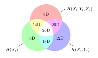
Figure 7: Dimension of the local cones obtained by allowing all accessible $m$-body terms.

cone	method	facets	classes
8D	CHM	104	7	(complete)
12D	$\operatorname{AFI_{1}}$	444	14	(complete)
14D	$\operatorname{AFI_{3}}$	566	22	(complete)
18D	RFD	888	22	(partial)
20D	RFD	496	17	(partial)
26D	ROA	1360	37	(partial)

Table 8: Number of discovered facets. The second number doesn’t count facets that can be obtained using a symmetry substitution.

Solving the 8D, 12D and 14D local cones

The convex hull method (CHM) turns out to be sufficient to compute complete descriptions of the 8D and 12D local cones in reasonable time. While the 8D cone is solved in a matter of seconds, the 12D cone already takes about 40 minutes to finish on a $2.4\text{\,}\mathrm{G}\mathrm{H}\mathrm{z}$ CPU and eats up several gigabytes of RAM. The 12D cone provides a prime example for the possible benefits of supplementing CHM with a single-level adjacent facet iteration (AFI). Using $\operatorname{AFI_{1}}$ cuts the calculation time down to about 20 seconds with a peak memory usage of roughly $180\text{\,}\mathrm{M}\mathrm{i}\mathrm{B}$. The 14D local cone was computed using a three-level AFI recursion in $37.5\text{\,}\mathrm{h}\text{/}$ taking $10\text{\,}\mathrm{GiB}\text{/}$ of RAM.

Solving the 18D local cone

The 18D subspace corresponding to the set of all one- and two-party entropies proves to be too much to be fully solved by CHM/AFI. However, this case admits to a treatment using a randomized facet discovery (RFD). We have achieved the best results with a 5-level recursion strategy $\operatorname{RFD_{5}}$.

Solving the 20D and 26D local cones

The largest marginal scenarios are 20D and 26D and thus well out of reach of CHM/AFI. However, the projection problem is computationally accessible using randomized strategies. In particular, we used the technique discussed in Sec. VII.4 (Algorithm 13) to improve upon outer approximations given by a list of known faces. There are several ways to obtain valid input constraints. The most naive is generate random ones by repeatedly applying the EPM based LP as discussed in Sec. IV.2. However, we could achieve a higher yield of facets by generating the outer constraints constructively from valid combinations of the input-space facets. This can be done systematically by exploiting simple observations about how elemental inequalities must be combined in order to obtain an expression in the output-space, see Section XVIII. A more physical approach is to directly improve upon a previously known outer approximation. In our case, we could use the extreme rays of the nonsignalling cone Chaves and Budroni (2016) as input constraints to find even a few more new facets.

XIII Witnessing tripartite nonlocality

Having obtained a list of inequalities characterizing a given marginal Bell scenario, our next interest is now which of these constraints can be violated by quantum mechanical correlations obtained from appropriate local measurements on a quantum state, and whether they can be used to indicate nonlocal correlations that are not detected by known nonlocality tests. Note that it’s a priori not clear whether a given inequality can witness quantum non-locality at all. Some of these inequalities are going to be trivial, in the sense that they represent elemental inequalities of the form (28) that are respected by any well defined probability distribution. Other inequalities, though not of elemental form, might still be trivial in the sense that they are respected by any non-signalling correlations Chaves and Budroni (2016); Budroni et al. (2016) (including quantum mechanical correlations).

Secondly, an important question in the multipartite scenario is whether one can witness non-locality if only few-body or even two-body measurements are available. As discussed before, from the physical perspective the relevance of these scenarios stems from the fact that there are typical setups where the available measurements are very restricted and thus the empirical data is limited to two-body correlators Tura et al. (2014). In this situation, we are also interested to see if any of our found tripartite Bell inequalities provides an advantage of the known bipartite nonlocality tests.

XIII.1 Bipartite nonlocality tests

There is a natural hierarchy to tackle this question. For setups in which each party can perform only two possible measurements, each with two outcomes, the canonical candidate for bipartite nonlocality tests is the CHSH inequality

$$2 \geq\lvert E(A_{1},B_{1})+E(A_{1},B_{2})$$

$$\quad+E(A_{2},B_{1})-E(A_{2},B_{2})\rvert.$$ (30)

Its entropic counterpart, the $$\operatorname{CHSH_{E}}$$ inequality

$$0 \leq H(A_{1},B_{1})+H(A_{1},B_{2})+H(A_{1},B_{1})$$

$$\quad-H(A_{2},B_{2})-H(A_{1})-H(B_{1})$$ (31)

is less tight but can also be applied in more general settings, e.g. if the number of outcomes is not fixed at two. In the case with more than 2 outcomes, another option is given by the CGLMP family of Bell inequalities constructed in Collins et al. (2002). These are constraints on the level of probabilities (like CHSH) that are applicable for the bipartite scenario with two measurements and $d$ outcomes per party (unlike CHSH). For example, the CGLMP inequality for a $d=3$ is:

$$2\geq\smash{\big{(}} {}+P(A_{1}=B_{1})+P(B_{1}=A_{2}+1)$$

$${}+P(A_{2}=B_{2})+P(B_{2}=A_{1})$$

$${}-P(A_{1}=B_{1}-1)-P(B_{1}=A_{2})$$

$${}-P(A_{2}=B_{2}-1)-P(B_{2}=A_{1}-1)\smash{\big{)}}.$$ (32)

All of the above bipartite constraints –CHSH, $\operatorname{CHSH_{E}}$ and CGLMP– are tied to a specified set of measurements. This means that even if the two-party locality constraints are satisfied, it is in principle possible that the quantum state could show bipartite non-local behaviour with a different set of measurements. Since entanglement is a necessary precondition for non-locality, one way to avoid this issue is to demand that all two-party subsystems are separable. In general, deciding whether a quantum state is separable is a non-trivial problem which has been shown to be NP-hard Lewenstein et al. (2000); Bruß (2002); Gurvits (2003); Gharibian (2010). A sufficient condition for entanglement, however, is the Peres–Horodecki criterion Peres (1996); Horodecki et al. (1996). It is also called PPT, which stands for positive partial transpose. Given a density matrix

$$\rho =\sum_{ijkl}p_{ijkl}\ket{i}\bra{j}\otimes\ket{k}\bra{l},$$

it states that if its partial transpose,

$$\rho^{T_{B}} =\sum_{ijkl}p_{ijkl}\ket{i}\bra{j}\otimes\ket{k}\bra{l},$$

has any negative eigenvalues, $\rho$ is guaranteed to be entangled. The choice of the subsystem B is arbitrary here. For $\mathbbm{C}_{2}\otimes\mathbbm{C}_{2}$ and $\mathbbm{C}_{2}\otimes\mathbbm{C}_{3}$ the criterion is both necessary and sufficient,

$$\rho\ \text{ separable} \Leftrightarrow\rho^{T_{B}}\geq 0,$$ (33)

which means that in a three-qubit system $\mathbbm{C}_{2}^{\otimes 3}$, by asserting PPT we can limit the search for non-local states to only states that are unentangled in any of the two-party subsystems. In the three-qutrit system $\mathbbm{C}_{3}^{\otimes 3}$ the criterion can be applied as well, but provides only a necessary condition for separability.

XIII.2 Search for non-locality witnesses

To the aim of answering the above questions we have searched for violations of each of the different inequality classes by means of numerical optimization. More details on the numerical method can be found in the Appendix XVII. We have considered projective measurements on tripartite quantum states composed by either qubits or qutrits, i.e. states that live in one of the spaces $\mathbbm{C}_{2}^{\otimes 3}$ or $\mathbbm{C}_{3}^{\otimes 3}$.

In both cases the search was first run unconstrained, i.e. without imposing that the violating quantum state should also fulfill further constraints on the level of two parties. As can be seen in Section XIII.2, in all investigated marginal scenarios, there are several facets (including non-trivial ones) for which we could not find quantum mechanical violations. Of course, this could be due to the fact that we are limiting the dimension of the considered quantum states and only looking to projective measurements. This is clearly illustrated by the fact that there are several inequalities for which we could not find violations considering qubits but which were violated by qutrit states. For instance, we found a qutrit violation for the inequality $I_{8}$ in the $26D$ scenario but failed to find any qubit violations.

system	constraints	12D		14D		18D		20D		26D
$\mathbbm{C}_{2}^{\otimes 3}$	none	$\kern-1.2pt\begin{aligned} l]{4}&I_{9},\ &&I_{10},\ &&I_{11},\ &&I_{12}\end{aligned}$		$\kern-1.2pt\begin{aligned} l]{4}&I_{5},\ &&I_{6},\ &&I_{7},\ &&I_{8},\\ &I_{9},\ &&I_{10},\ &&I_{15},\ &&I_{17},\\ &I_{18},\ &&I_{20},\ &&I_{21}\end{aligned}$		$\kern-1.2pt\begin{aligned} l]{4}&I_{3},\ &&I_{4},\ &&I_{7},\ &&I_{10},\\ &I_{13},\ &&I_{18}\end{aligned}$		$\kern-1.2pt\begin{aligned} l]{4}&I_{8},\ &&I_{11},\ &&I_{12},\ &&I_{13},\\ &I_{14},\ &&I_{15},\ &&I_{16}\end{aligned}$		$\kern-1.2pt\begin{aligned} l]{5}&I_{1},\ &&I_{17},\ &&I_{23},\ &&I_{24},\ &&I_{26},\\ &I_{27},\ &&I_{28},\ &&I_{29},\ &&I_{31},\ &&I_{32},\\ &I_{34},\ &&I_{35},\ &&I_{36}\end{aligned}$
	$\operatorname{CHSH_{E}}$			$\kern-1.2pt\begin{aligned} l]{4}&I_{6},\ &&I_{7},\ &&I_{9},\ &&I_{10},\\ &I_{15},\ &&I_{17},\ &&I_{18},\ &&I_{21}\end{aligned}$				$\kern-1.2pt\begin{aligned} l]{4}&I_{8},\ &&I_{11},\ &&I_{12},\ &&I_{13},\\ &I_{14},\ &&I_{15},\ &&I_{16}\end{aligned}$		$\kern-1.2pt\begin{aligned} l]{5}&I_{17},\ &&I_{23},\ &&I_{26},\ &&I_{27},\ &&I_{28},\\ &I_{29},\ &&I_{31},\ &&I_{32},\ &&I_{34},\ &&I_{35},\\ &I_{36}\end{aligned}$
	CHSH			$\kern-1.2pt\begin{aligned} l]{4}&I_{17},\ &&I_{18},\ &&I_{21}\end{aligned}$				$\kern-1.2pt\begin{aligned} l]{4}&I_{8},\ &&I_{11},\ &&I_{12},\ &&I_{13},\\ &I_{14},\ &&I_{15},\ &&I_{16}\end{aligned}$		$\kern-1.2pt\begin{aligned} l]{5}&I_{17},\ &&I_{23},\ &&I_{26},\ &&I_{27},\ &&I_{28},\\ &I_{29},\ &&I_{34},\ &&I_{35},\ &&I_{36}\end{aligned}$
	PPT			$\kern-1.2pt\begin{aligned} l]{4}&I_{18}\end{aligned}$				$\kern-1.2pt\begin{aligned} l]{4}&I_{8},\ &&I_{11},\ &&I_{12},\ &&I_{13},\\ &I_{14},\ &&I_{15}\end{aligned}$		$\kern-1.2pt\begin{aligned} l]{5}&I_{17},\ &&I_{26},\ &&I_{27},\ &&I_{28},\ &&I_{29},\\ &I_{34},\ &&I_{35},\ &&I_{36}\end{aligned}$
$\mathbbm{C}_{3}^{\otimes 3}$	none	$\kern-1.2pt\begin{aligned} l]{4}&I_{9},\ &&I_{10},\ &&I_{11},\ &&I_{12}\end{aligned}$		$\kern-1.2pt\begin{aligned} l]{4}&I_{5},\ &&I_{6},\ &&I_{7},\ &&I_{8},\\ &I_{9},\ &&I_{10},\ &&I_{15},\ &&I_{17},\\ &I_{18},\ &&I_{20},\ &&I_{21}\end{aligned}$		$\kern-1.2pt\begin{aligned} l]{4}&I_{3},\ &&I_{4},\ &&I_{7},\ &&I_{10},\\ &I_{13},\ &&I_{18}\end{aligned}$		$\kern-1.2pt\begin{aligned} l]{4}&I_{8},\ &&I_{11},\ &&I_{12},\ &&I_{13},\\ &I_{14},\ &&I_{15},\ &&I_{16}\end{aligned}$		$\kern-1.2pt\begin{aligned} l]{5}&I_{1},\ &&I_{8},\ &&I_{12},\ &&I_{17},\ &&I_{23},\\ &I_{24},\ &&I_{26},\ &&I_{27},\ &&I_{28},\ &&I_{29},\\ &I_{31},\ &&I_{32},\ &&I_{34},\ &&I_{35},\ &&I_{36}\end{aligned}$
	CGLMP	$\kern-1.2pt\begin{aligned} l]{4}&I_{9},\ &&I_{10},\ &&I_{11},\ &&I_{12}\end{aligned}$		$\kern-1.2pt\begin{aligned} l]{4}&I_{5},\ &&I_{6},\ &&I_{7},\ &&I_{8},\\ &I_{9},\ &&I_{10},\ &&I_{15},\ &&I_{17},\\ &I_{18},\ &&I_{20},\ &&I_{21}\end{aligned}$		$\kern-1.2pt\begin{aligned} l]{4}&I_{3},\ &&I_{4},\ &&I_{7},\ &&I_{10},\\ &I_{13},\ &&I_{18}\end{aligned}$		$\kern-1.2pt\begin{aligned} l]{4}&I_{8},\ &&I_{11},\ &&I_{12},\ &&I_{13},\\ &I_{14},\ &&I_{15},\ &&I_{16}\end{aligned}$		$\kern-1.2pt\begin{aligned} l]{5}&I_{1},\ &&I_{8},\ &&I_{12},\ &&I_{17},\ &&I_{23},\\ &I_{24},\ &&I_{26},\ &&I_{27},\ &&I_{28},\ &&I_{29},\\ &I_{31},\ &&I_{32},\ &&I_{34},\ &&I_{35},\ &&I_{36}\end{aligned}$
	$\operatorname{CHSH_{E}}$			$\kern-1.2pt\begin{aligned} l]{4}&I_{5},\ &&I_{6},\ &&I_{7},\ &&I_{8},\\ &I_{9},\ &&I_{10},\ &&I_{15},\ &&I_{17},\\ &I_{18},\ &&I_{21}\end{aligned}$		$\kern-1.2pt\begin{aligned} l]{4}&I_{4},\ &&I_{7},\ &&I_{10},\ &&I_{18}\end{aligned}$		$\kern-1.2pt\begin{aligned} l]{4}&I_{8},\ &&I_{11},\ &&I_{12},\ &&I_{13},\\ &I_{14},\ &&I_{15},\ &&I_{16}\end{aligned}$		$\kern-1.2pt\begin{aligned} l]{5}&I_{8},\ &&I_{12},\ &&I_{17},\ &&I_{23},\ &&I_{24},\\ &I_{26},\ &&I_{27},\ &&I_{28},\ &&I_{29},\ &&I_{31},\\ &I_{32},\ &&I_{34},\ &&I_{35},\ &&I_{36}\end{aligned}$
	PPT			$\kern-1.2pt\begin{aligned} l]{4}&I_{17}\end{aligned}$				$\kern-1.2pt\begin{aligned} l]{4}&I_{8},\ &&I_{12},\ &&I_{14},\ &&I_{15}\end{aligned}$		$\kern-1.2pt\begin{aligned} l]{5}&I_{17},\ &&I_{26},\ &&I_{27},\ &&I_{28},\ &&I_{29},\\ &I_{34},\ &&I_{35},\ &&I_{36}\end{aligned}$

Table 9: Non-locality witnesses of the 12D/14D/18D/20D/26D cone that satisfy the given constraint on all two party subsystems. No non-locality witnesses have been identified for the 8D cone. The inequalities $I_{k}\boldsymbol{h}\geq 0$ are listed in Section XVI. Recall that 14D/20D/26D do involve three-body correlators, while 12D/18D get along with two-body correlators.

For each member of this established set of nonlocality witnesses we proceeded by searching for nonlocal states while imposing all symmetries of the known bipartite locality constraints appropriate for the respective system. Specifically, for the three-qubit system $\operatorname{CHSH_{E}}$, CHSH and the PPT criterion are applicable and provide increasingly tight bounds in this order. The three-qutrit system was subjected to CGLMP, $\operatorname{CHSH_{E}}$ and PPT. The resulting sets of non-locality witnesses are listed in Section XIII.2.

We start by observing that the tripartite Bell inequalities seem to be more advantageous compared to bipartite tests when going to higher dimensional quantum systems, i.e. systems with more outcomes. This is shown by the fact that, by imposing CHSH or $\operatorname{CHSH_{E}}$, we could find much fewer inequality violations with qubits. Of particular relevance is the usefulness of our inequalities as nonlocality witnesses in the case that we have access to only two-body correlators (12D, 18D). As can be seen in Section XIII.2, using qutrit states (and 3 measurement outcomes) we found examples of correlations such that the marginals violate neither $\operatorname{CHSH_{E}}$ nor CGLMP, yet do violate some of the inequalities characterizing the 18D local cone. That is, if we just trace out one of the parties (returning to a bipartite Bell scenario) the correlations are classical. However, if instead we look at all available bipartite information (considering the 3 pairs of bipartite distributions) we can witness its non-locality.

Finally, as pointed out by Wurflinger et al. Würflinger et al. (2012), multipartite entanglement can be inferred from marginal probabilities that are local in all two-party subsystems. We now ask a related question: Can our Bell inequalities detect the non-locality of tripartite states even if all two-party subsystems are separable? In such a case, no bipartite test can detect the nonlocality of the state. Unfortunately, we could only achieve violations with separable/PPT marginals (for instance, a GHZ state of the inequalities that do involve 3-body terms. It thus remain an open question whether the results in Würflinger et al. (2012) can be extended in its full generality for entropic Bell inequalities.

XIV Discussion and Outlook

The characterization of the set of correlations/probability distributions of a given marginal scenario is of central relevance in a variety of fields. Algebraic geometry Huynh et al. (1990); Geiger and Meek (1999); Garcia et al. (2005) and quantifier elimination methods Lassez and Lassez (1990); Davenport and Heintz (1988); Monniaux (2010) provide a very general tool for tackling the problem that in practice, unfortunately, is limited to very few cases of interest due to its double exponential computational complexity. In the particular case where such sets define convex regions such as the polytopes arising in the study of Bell non-locality Pitowsky (1989) or the entropy cones arising in the study of information theory Yeung (2008) or causal inference Chaves et al. (2014a, b), the complexity of the task is certainly reduced since the often efficient tools from convex optimization theory can be employed. Yet, even in the convex case, we also often encounter situations and marginal scenarios out of reach of current algorithms.

Within this context, we have provided a review of known algorithms for the projection of convex polyhedra and also proposed a new one, that we call adjacent facet iteration. To show its relevance and compare it with previous methods we have employed it for the derivation of entropic Bell inequalities in a tripartite scenario. As discussed, our method provided a significant time improvement over other usual methods and in some cases allowed for the characterization of marginal scenarios outside the reach of other algorithms. With that we managed to derive several novel tripartite Bell inequalities that furthermore are facets of the associated entropy cone. Of particular relevance, are the inequalities involving at most bipartite information, that is, involving at most two observables. To our knowledge, these are first entropic Bell inequalities of this kind, thus extending the results of Tura et al. (2014) in the context of Bell inequalities well suited for the analysis of many-body systems. Further, we have shown that such inequalities can be violated by probability distributions that appear to be local by other standard bipartite tests such as the CHSH and CGLMP inequalities Clauser et al. (1969b); Collins et al. (2002), an extension to the entropic regime of the results in Würflinger et al. (2012) and that clearly show the relevance of these new inequalities.

As for future research, we believe there are few promising directions. For instance, multipartite Bell inequalities involving at most two-body correlations have been proposed Tura et al. (2014) to probe the non-classicality of many-body systems where the measurement of observables is very limited (see for instance an experimental realization of this idea in Schmied et al. (2016)). Most of such inequalities, however, are derived for the particular of binary measurement outcomes. In contrast, since entropic Bell inequalities are valid for an arbitrary number of outcomes, they could provide a natural venue to extend such results for quantum systems and measurements of higher dimensions. In turn, we believe that the computational method we propose here could also find applications in the characterization of causal networks beyond the Bell network (see for instance Chaves et al. (2014a); Henson et al. (2014); Weilenmann and Colbeck (2017)). As an illustration of that, we provide in the Appendix the full characterization of two common ancestor causal structures that generalize the triangle causal structure Steudel et al. (2010) that has been the focus of much research in quantum foundations recently Fritz (2012); Chaves et al. (2014a); Henson et al. (2014); Wolfe et al. (2016). We hope our results might trigger further research on this direction.

Appendix

XV Characterizing common-ancestors causal structures

In addition to the Bell scenarios discussed in the previous sections, we have also investigated applications for so-called pairwise hidden ancestor models.

The triangle scenario $\mathcal{C}_{3}$ (Figure 10(a)) is a prominent causal model for the relationship of three observable variables. It has been considered both in classical context Steudel and Ay (2010) as well as quantum non-locality Branciard et al. (2012); Fritz (2012). Contrary to the corresponding single-common-ancestor model (Figure 10(b)), it exhibits non-trivial constraints and is therefore preferred by Occam’s razor if both models are compatible with given empirical data.

Figure 10: Common ancestor models

(a) Triangle $\mathcal{C}_{3}$

(b) Single ancestor

(c) Square $\mathcal{C}_{4}$

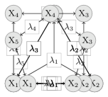
(d) Pentagon $\mathcal{C}_{5}$

The triangle can be generalized as a regular polygone $\mathcal{C}_{n}$, see the square and pentagon in Figure 10(c) and Figure 10(d). The entropic constraints associated with $\mathcal{C}_{n}$ are the mutual independence of the ancestors $H(\lambda_{\Omega})=\sum_{i\in\Omega}H(\lambda_{i})$ and the local Markov conditions

$$0=I(X_{i}:X_{\Omega-\{i\}},\lambda_{\Omega-\operatorname{Pa}_{i}}\ooalign{$\phantom{{},{}}$\cr$|$}\lambda_{\operatorname{Pa}_{i}}),$$

for all observable variables $X_{i}$, where $\Omega=[n]$ and $\operatorname{Pa}_{i}=\{i,\,(i\kern-2.0pt\mod n)+1\}$.

In Fritz and Chaves (2013), the authors employ a Fourier-Motzkin elimination using the PORTA open source software package in an attempt to compute the projection of $\mathcal{C}_{3}$ to the marginal scenario $\mathcal{M}=2^{X_{\Omega}}$ that includes all observable terms. However, their computations did not complete – which shows that even such a simple model can prove difficult for FME if not using proper protection redundancy elimination. This particular problem is solved in Chaves et al. (2014a), showing that there are only three non-trivial classes of inequalities:

$$0 \leq 4H_{12}+4H_{13}+4H_{23}-2H_{123}-5H_{1}-5H_{2}-5H_{3},$$

$$0 \leq 3H_{12}+2H_{13}+2H_{23}-\phantom{2}H_{123}-3H_{1}-3H_{2}-3H_{3},$$

$$0 \leq H_{12}+H_{23}-H_{1}-H_{2}-H_{3}.$$

We now extend these results by computing the full projection of the square $\mathcal{C}_{4}$ and pentagon $\mathcal{C}_{5}$. The results are obtained using an FM elimination with full LP-based redundancy removal. The implementation can be found in Gläßle (2016b). All classes of facets can be found online Gläßle (2016a) and are additionally listed in Section XVI. In total, the marginal cone of $\mathcal{C}_{4}$ has 12 distinct classes of facets, the $\mathcal{C}_{5}$ marginal cone has 39 classes of facets.

Starting from a system with no redundancies, the computations take $7.4\text{\,}\mathrm{s}\text{/}$ and $340\text{\,}\mathrm{s}\text{/}$ for $\mathcal{C}_{4}$ and $\mathcal{C}_{5}$, respectively (on a usual desktop PC). This underlines how LP-based redundancy removal can be a major advantage in performing FM eliminations.

XVI List of inequalities

In the following we list the facets that were found using the techniques discussed in the main text. Note that we list expressions $I_{k}$ which should be read as inequalities $I_{k}\geq 0$. Furthermore, if multiple inequalities are equivalent by a symmetry of the cone (i.e. relabeling of variables), we list only one representative. The data can also be found online in the repository of the pystif software package Gläßle (2016a).

XVI.1 Machine readable data

We include quick response (QR) codes to allow easy data acquisition. Due to the capacity limitations of QR codes the data is gzipped. The raw data files can be unpacked with a wide range of popular compression software such as 7z on Windows or the prevalent gunzip tool on UNIX-like systems:

gunzip -c raw.dat > friendly.txt

The unzipped data is also directly attached to the PDF and can be accessed by clicking on the QR code images. The uncompressed data is a self-documenting text file that can e.g. be directly used as input file for any of the pystif utilities. However, the full pystif stack is not required – the text format is suitable for machine reading and easy to parse. For example, in python you can use

⬇

>>> numpy.loadtxt(’friendly.txt’)

to obtain a numpy array whose row vectors $\boldsymbol{I}$ correspond to linear inequalities $\boldsymbol{I}\cdot\boldsymbol{h}\geq 0$ where $\boldsymbol{h}$ is an entropy vector. The column order is generally based on number of arguments and party affiliation but is also documented within the file.

XVI.2 8D cone

Full characterization of the marginal cone with all one-body terms for the tripartite Bell scenario.

$$I_{0}=H(A_{1}\,B_{1}\,C_{2})$$

$$I_{1}=H(A_{1}\,B_{2}\,C_{1})+H(A_{2}\,B_{1}\,C_{2})-H(A_{1}\,B_{2}\,C_{2})$$

$$I_{2}=H(A_{1}\,B_{1}\,C_{2})+H(A_{2}\,B_{2}\,C_{2})-H(A_{2}\,B_{1}\,C_{2})$$

$$I_{3}=H(A_{1}\,B_{2}\,C_{2})+H(A_{2}\,B_{1}\,C_{2})+H(A_{2}\,B_{2}\,C_{1})-H(A_{1}\,B_{1}\,C_{1})-H(A_{2}\,B_{2}\,C_{2})$$

$$I_{4}=H(A_{1}\,B_{1}\,C_{2})+H(A_{1}\,B_{2}\,C_{1})+H(A_{2}\,B_{2}\,C_{2})-2H(A_{1}\,B_{2}\,C_{2})$$

$$I_{5}=H(A_{1}\,B_{1}\,C_{2})+H(A_{1}\,B_{2}\,C_{1})+H(A_{2}\,B_{2}\,C_{2})-H(A_{1}\,B_{2}\,C_{2})-H(A_{2}\,B_{2}\,C_{1})$$

$$I_{6}=2H(A_{1}\,B_{1}\,C_{1})+2H(A_{2}\,B_{1}\,C_{2})+2H(A_{2}\,B_{2}\,C_{1})-H(A_{1}\,B_{1}\,C_{2})-H(A_{1}\,B_{2}\,C_{1})-H(A_{2}\,B_{1}\,C_{1})-H(A_{2}\,B_{2}\,C_{2})$$

Figure 11: 8D cone

XVI.3 12D cone

Full characterization of the marginal cone with all two-body terms for the tripartite Bell scenario.

$$I_{0}=H(B_{1}\,C_{2})+H(B_{2}\,C_{1})-H(B_{2}\,C_{2})$$

$$I_{1}=H(A_{1}\,B_{2})+H(B_{1}\,C_{2})-H(A_{1}\,C_{2})$$

$$I_{2}=H(A_{1}\,B_{2})+H(B_{1}\,C_{2})-H(B_{2}\,C_{2})$$

$$I_{3}=H(A_{1}\,B_{1})+H(B_{1}\,C_{2})-H(A_{1}\,C_{2})$$

$$I_{4}=H(A_{1}\,B_{1})+H(A_{2}\,B_{2})+H(B_{2}\,C_{1})-H(A_{1}\,B_{2})-H(A_{2}\,C_{1})$$

$$I_{5}=H(A_{1}\,B_{1})+H(A_{2}\,C_{2})+H(B_{1}\,C_{2})-H(A_{2}\,B_{1})-H(A_{1}\,C_{2})$$

$$I_{6}=H(A_{1}\,B_{1})+H(A_{2}\,C_{2})+H(B_{2}\,C_{2})-H(A_{2}\,B_{2})-H(A_{1}\,C_{2})$$

$$I_{7}=H(A_{1}\,B_{1})+H(A_{2}\,B_{2})+H(A_{2}\,C_{2})+H(B_{1}\,C_{2})-H(A_{2}\,B_{1})-H(A_{1}\,C_{2})-H(B_{2}\,C_{2})$$

$$I_{8}=H(A_{1}\,B_{1})+H(A_{2}\,C_{1})+H(B_{1}\,C_{2})+H(B_{2}\,C_{1})-H(A_{2}\,B_{2})-H(A_{1}\,C_{2})-H(B_{1}\,C_{1})$$

$$I_{9}=H(A_{1}\,B_{1})+H(A_{2}\,B_{1})+H(A_{2}\,B_{2})+H(A_{1}\,C_{1})+H(A_{1}\,C_{2})+H(B_{2}\,C_{1})+H(B_{2}\,C_{2})-3H(A_{1}\,B_{2})-H(A_{2}\,C_{1})-H(B_{1}\,C_{2})$$

$$I_{10}=2H(A_{1}\,B_{1})+2H(B_{1}\,C_{2})+H(A_{1}\,C_{1})+H(A_{2}\,C_{1})+H(A_{2}\,C_{2})-3H(A_{1}\,C_{2})-H(A_{2}\,B_{1})-H(B_{1}\,C_{1})$$

$$I_{11}=3H(A_{1}\,B_{1})+2H(B_{1}\,C_{2})+H(A_{1}\,C_{1})+H(A_{2}\,C_{1})+H(A_{2}\,C_{2})+H(B_{2}\,C_{1})+H(B_{2}\,C_{2})-4H(A_{1}\,C_{2})-2H(B_{1}\,C_{1})-H(A_{2}\,B_{2})$$

$$I_{12}=2H(A_{2}\,B_{2})+2H(A_{1}\,C_{1})+H(A_{1}\,B_{2})+H(A_{2}\,B_{1})+H(A_{1}\,C_{2})+H(A_{2}\,C_{1})+H(B_{1}\,C_{1})+H(B_{1}\,C_{2})+H(B_{2}\,C_{2})-4H(B_{2}\,C_{1})-2H(A_{1}\,B_{1})-2H(A_{2}\,C_{2})$$

$$I_{13}=3H(B_{2}\,C_{2})+2H(A_{2}\,B_{2})+2H(A_{1}\,C_{2})+H(A_{1}\,B_{1})+H(A_{2}\,B_{1})+H(A_{1}\,C_{1})+H(A_{2}\,C_{1})-4H(A_{2}\,C_{2})-3H(A_{1}\,B_{2})-H(B_{1}\,C_{1})$$

Figure 12: 12D cone

XVI.4 14D cone

Full characterization of the marginal cone with all one- and three-body terms for the tripartite Bell scenario.

$$I_{0}=H(B_{1})$$

$$I_{1}=H(A_{1})+H(B_{1})+H(C_{2})-H(A_{1}\,B_{1}\,C_{2})$$

$$I_{2}=H(A_{2}\,B_{2}\,C_{2})-H(B_{2})$$

$$I_{3}=H(A_{2}\,B_{1}\,C_{2})+H(A_{1})-H(A_{1}\,B_{1}\,C_{2})$$

$$I_{4}=H(A_{1}\,B_{2}\,C_{2})+H(A_{2}\,B_{2}\,C_{1})-H(A_{1}\,B_{2}\,C_{1})-H(B_{2})$$

$$I_{5}=H(A_{1}\,B_{2}\,C_{2})+H(A_{2}\,B_{1}\,C_{2})+H(A_{2}\,B_{2}\,C_{2})-H(A_{1}\,B_{1}\,C_{2})-H(A_{2})-H(B_{2})$$

$$I_{6}=H(A_{1}\,B_{2}\,C_{1})+H(A_{2}\,B_{1}\,C_{1})+H(A_{2}\,B_{2}\,C_{2})-H(A_{1}\,B_{1}\,C_{2})-H(B_{2})-H(C_{1})$$

$$I_{7}=H(A_{1}\,B_{1}\,C_{1})+H(A_{2}\,B_{2}\,C_{1})+H(A_{2}\,B_{2}\,C_{2})-H(A_{1}\,B_{1}\,C_{2})-H(B_{2})-H(C_{1})$$

$$I_{8}=H(A_{1}\,B_{1}\,C_{1})+H(A_{2}\,B_{2}\,C_{1})+H(A_{2}\,B_{2}\,C_{2})-H(A_{2}\,B_{1}\,C_{2})-H(B_{2})-H(C_{1})$$

$$I_{9}=2H(A_{2}\,B_{2}\,C_{2})+H(A_{1}\,B_{2}\,C_{1})+H(A_{2}\,B_{1}\,C_{1})-H(A_{1}\,B_{1}\,C_{1})-H(A_{2}\,B_{2}\,C_{1})-H(A_{2})-H(B_{2})$$

$$I_{10}=2H(A_{2}\,B_{2}\,C_{2})+H(A_{1}\,B_{2}\,C_{1})+H(A_{2}\,B_{1}\,C_{1})-H(A_{1}\,B_{1}\,C_{2})-H(A_{2}\,B_{2}\,C_{1})-H(A_{2})-H(B_{2})$$

$$I_{11}=H(A_{1}\,B_{1}\,C_{1})+H(A_{1}\,B_{2}\,C_{2})+H(A_{2}\,B_{1}\,C_{2})+H(A_{2}\,B_{2}\,C_{2})+H(C_{2})-H(A_{1}\,B_{1}\,C_{2})-H(A_{1}\,B_{2}\,C_{1})-H(A_{2})-H(B_{2})$$

$$I_{12}=H(A_{1}\,B_{1}\,C_{1})+H(A_{1}\,B_{2}\,C_{2})+H(A_{2}\,B_{1}\,C_{1})+H(A_{2}\,B_{1}\,C_{2})+H(B_{1})-H(A_{1}\,B_{1}\,C_{2})-H(A_{2}\,B_{2}\,C_{1})-H(A_{2})-H(C_{1})$$

$$I_{13}=2H(A_{1}\,B_{1}\,C_{1})+H(A_{1}\,B_{2}\,C_{2})+H(A_{2}\,B_{1}\,C_{1})+H(A_{2}\,B_{1}\,C_{2})-H(A_{1}\,B_{1}\,C_{2})-H(A_{2}\,B_{2}\,C_{1})-H(A_{1})-H(A_{2})-H(C_{1})$$

$$I_{14}=2H(A_{1}\,B_{1}\,C_{1})+H(A_{1}\,B_{2}\,C_{2})+H(A_{2}\,B_{1}\,C_{1})+H(A_{2}\,B_{1}\,C_{2})-H(A_{1}\,B_{1}\,C_{2})-H(A_{2}\,B_{2}\,C_{2})-H(A_{1})-H(A_{2})-H(C_{1})$$

$$I_{15}=2H(A_{2}\,B_{1}\,C_{1})+H(A_{1}\,B_{2}\,C_{1})+H(A_{1}\,B_{2}\,C_{2})+H(A_{2}\,B_{2}\,C_{2})-2H(A_{1}\,B_{1}\,C_{2})-H(A_{2})-H(B_{2})-H(C_{1})$$

$$I_{16}=H(A_{1}\,B_{1}\,C_{1})+H(A_{1}\,B_{2}\,C_{2})+H(A_{2}\,B_{1}\,C_{1})+H(A_{2}\,B_{1}\,C_{2})+H(A_{2}\,B_{2}\,C_{2})-H(A_{1}\,B_{1}\,C_{2})-H(A_{1}\,B_{2}\,C_{1})-H(A_{2})-H(B_{2})-H(C_{1})$$

$$I_{17}=2H(A_{1}\,B_{1}\,C_{1})+2H(A_{1}\,B_{2}\,C_{2})+2H(A_{2}\,B_{2}\,C_{1})-2H(A_{2}\,B_{1}\,C_{2})-H(A_{1}\,B_{2}\,C_{1})-H(A_{1})-H(B_{2})-H(C_{1})$$

$$I_{18}=H(A_{1}\,B_{1}\,C_{1})+H(A_{1}\,B_{2}\,C_{1})+H(A_{1}\,B_{2}\,C_{2})+H(A_{2}\,B_{1}\,C_{1})+H(A_{2}\,B_{1}\,C_{2})+H(A_{2}\,B_{2}\,C_{2})-3H(A_{1}\,B_{1}\,C_{2})-H(A_{2})-H(B_{2})-H(C_{1})$$

$$I_{19}=H(A_{1}\,B_{1}\,C_{1})+H(A_{1}\,B_{2}\,C_{1})+H(A_{1}\,B_{2}\,C_{2})+H(A_{2}\,B_{1}\,C_{1})+H(A_{2}\,B_{1}\,C_{2})+H(A_{2}\,B_{2}\,C_{2})-2H(A_{2}\,B_{2}\,C_{1})-H(A_{1}\,B_{1}\,C_{2})-H(A_{2})-H(B_{2})-H(C_{1})$$

$$I_{20}=2H(A_{1}\,B_{1}\,C_{1})+2H(A_{1}\,B_{2}\,C_{2})+2H(A_{2}\,B_{1}\,C_{2})+H(A_{2}\,B_{1}\,C_{1})-2H(A_{2}\,B_{2}\,C_{1})-H(A_{1}\,B_{1}\,C_{2})-H(A_{1})-H(A_{2})-H(C_{1})-H(C_{2})$$

$$I_{21}=2H(A_{1}\,B_{2}\,C_{2})+2H(A_{2}\,B_{2}\,C_{1})+H(A_{1}\,B_{1}\,C_{1})+H(A_{2}\,B_{1}\,C_{1})+H(A_{2}\,B_{1}\,C_{2})-3H(A_{1}\,B_{1}\,C_{2})-2H(B_{2})-H(A_{2})-H(C_{1})$$

Figure 13: 14D cone

XVI.5 18D cone

Listing of discovered facets of the marginal cone of the tripartite Bell scenario where the marginal scenario contains all one- and two-body terms. These facets do not provide a full characterization.

$$I_{0}=H(B_{1})+H(C_{1})-H(B_{1}\,C_{1})$$

$$I_{1}=H(A_{1}\,B_{2})-H(B_{2})$$

$$I_{2}=H(A_{1}\,B_{2})+H(A_{1}\,C_{1})-H(B_{2}\,C_{1})-H(A_{1})$$

$$I_{3}=H(A_{1}\,C_{1})+H(A_{2}\,C_{1})+H(A_{2}\,C_{2})-H(A_{1}\,C_{2})-H(A_{2})-H(C_{1})$$

$$I_{4}=H(A_{1}\,B_{2})+H(A_{1}\,C_{2})+H(A_{2}\,C_{1})+H(A_{2}\,C_{2})+H(B_{2}\,C_{1})-H(A_{1}\,C_{1})-H(B_{2}\,C_{2})-H(A_{1})-H(A_{2})-H(C_{1})$$

$$I_{5}=H(A_{1}\,B_{2})+H(A_{1}\,C_{1})+H(A_{2}\,C_{1})+H(A_{2}\,C_{2})+H(B_{2}\,C_{2})-H(A_{2}\,B_{2})-H(A_{1}\,C_{2})-H(A_{2})-H(B_{2})-H(C_{1})$$

$$I_{6}=H(A_{1}\,B_{2})+H(A_{2}\,B_{2})+H(A_{1}\,C_{1})+H(A_{2}\,C_{1})+H(A_{2}\,C_{2})-H(A_{1}\,C_{2})-H(B_{2}\,C_{1})-H(A_{2})-H(B_{2})-H(C_{1})$$

$$I_{7}=H(A_{1}\,C_{1})+H(A_{1}\,C_{2})+H(A_{2}\,C_{1})+H(B_{1}\,C_{1})+H(B_{1}\,C_{2})-H(A_{1}\,B_{1})-H(A_{2}\,C_{2})-2H(C_{1})-H(C_{2})$$

$$I_{8}=H(A_{1}\,B_{1})+H(A_{1}\,B_{2})+H(A_{2}\,B_{1})+H(A_{2}\,B_{2})+H(A_{1}\,C_{2})+H(B_{1}\,C_{1})-H(A_{2}\,C_{2})-H(B_{2}\,C_{1})-2H(A_{1})-H(A_{2})-H(B_{1})$$

$$I_{9}=H(A_{1}\,B_{2})+H(A_{2}\,B_{2})+H(A_{1}\,C_{2})+H(A_{2}\,C_{1})+H(B_{1}\,C_{1})+H(B_{1}\,C_{2})-H(A_{1}\,C_{1})-H(A_{2}\,C_{2})-H(A_{1})-H(B_{1})-H(B_{2})-H(C_{1})$$

$$I_{10}=H(A_{1}\,B_{1})+H(A_{1}\,B_{2})+H(A_{2}\,B_{2})+H(A_{1}\,C_{2})+H(A_{2}\,C_{1})+H(A_{2}\,C_{2})+H(B_{1}\,C_{1})-H(A_{2}\,B_{1})-H(A_{1}\,C_{1})-H(B_{2}\,C_{2})-2H(A_{1})-H(A_{2})-H(C_{1})$$

$$I_{11}=H(A_{1}\,B_{2})+H(A_{2}\,B_{1})+H(A_{2}\,B_{2})+H(A_{1}\,C_{2})+H(B_{1}\,C_{1})+H(B_{1}\,C_{2})+H(B_{2}\,C_{1})-H(A_{1}\,B_{1})-H(A_{2}\,C_{1})-H(B_{2}\,C_{2})-H(A_{1})-H(A_{2})-H(B_{1})-H(C_{1})$$

$$I_{12}=H(A_{1}\,B_{1})+H(A_{1}\,B_{2})+H(A_{2}\,B_{2})+H(A_{2}\,C_{1})+H(A_{2}\,C_{2})+H(B_{1}\,C_{1})+H(B_{1}\,C_{2})-H(A_{2}\,B_{1})-H(A_{1}\,C_{1})-H(B_{2}\,C_{2})-H(A_{1})-H(A_{2})-H(B_{1})-H(C_{1})$$

$$I_{13}=H(A_{1}\,B_{2})+H(A_{2}\,B_{2})+H(A_{1}\,C_{2})+H(A_{2}\,C_{1})+H(A_{2}\,C_{2})+H(B_{1}\,C_{1})+H(B_{1}\,C_{2})-H(A_{2}\,B_{1})-H(A_{1}\,C_{1})-H(B_{2}\,C_{2})-H(A_{1})-H(A_{2})-H(C_{1})-H(C_{2})$$

$$I_{14}=H(A_{1}\,B_{2})+H(A_{2}\,B_{1})+H(A_{2}\,B_{2})+H(A_{1}\,C_{1})+H(B_{1}\,C_{1})+H(B_{1}\,C_{2})+H(B_{2}\,C_{2})-H(A_{1}\,C_{2})-H(A_{2}\,C_{2})-H(B_{2}\,C_{1})-2H(B_{1})-H(A_{1})-H(B_{2})$$

$$I_{15}=H(A_{1}\,B_{2})+H(A_{2}\,B_{1})+H(A_{2}\,B_{2})+H(A_{1}\,C_{1})+H(A_{1}\,C_{2})+H(B_{1}\,C_{1})+H(B_{1}\,C_{2})-H(A_{1}\,B_{1})-H(A_{2}\,C_{1})-H(A_{2}\,C_{2})-H(A_{1})-H(B_{1})-H(B_{2})-H(C_{1})$$

$$I_{16}=H(A_{1}\,B_{2})+H(A_{2}\,B_{1})+H(A_{2}\,B_{2})+H(B_{1}\,C_{1})+H(B_{1}\,C_{2})+H(B_{2}\,C_{1})+H(B_{2}\,C_{2})-H(A_{1}\,B_{1})-H(A_{2}\,C_{1})-H(A_{2}\,C_{2})-2H(B_{2})-H(B_{1})-H(C_{1})$$

$$I_{17}=2H(B_{1}\,C_{2})+H(A_{1}\,B_{2})+H(A_{2}\,B_{1})+H(A_{2}\,B_{2})+H(A_{1}\,C_{2})+H(B_{1}\,C_{1})+H(B_{2}\,C_{1})-H(A_{1}\,B_{1})-H(A_{2}\,C_{1})-H(A_{2}\,C_{2})-2H(B_{1})-H(A_{1})-H(B_{2})-H(C_{1})$$

$$I_{18}=2H(A_{1}\,B_{2})+2H(B_{1}\,C_{1})+H(A_{1}\,B_{1})+H(A_{2}\,B_{2})+H(A_{1}\,C_{2})+H(A_{2}\,C_{1})+H(A_{2}\,C_{2})+H(B_{1}\,C_{2})+H(B_{2}\,C_{1})-2H(A_{1}\,C_{1})-2H(B_{2}\,C_{2})-H(A_{2}\,B_{1})-2H(A_{1})-2H(C_{1})-H(A_{2})-H(B_{1})$$

$$I_{19}=2H(A_{2}\,B_{2})+2H(A_{2}\,C_{2})+2H(B_{1}\,C_{1})+H(A_{1}\,B_{1})+H(A_{1}\,B_{2})+H(A_{1}\,C_{2})+H(A_{2}\,C_{1})+H(B_{1}\,C_{2})+H(B_{2}\,C_{1})-2H(A_{2}\,B_{1})-2H(A_{1}\,C_{1})-H(B_{2}\,C_{2})-2H(B_{2})-2H(C_{1})-2H(C_{2})-H(A_{1})$$

$$I_{20}=2H(A_{2}\,C_{1})+2H(A_{2}\,C_{2})+2H(B_{1}\,C_{1})+H(A_{1}\,B_{1})+H(A_{1}\,B_{2})+H(A_{2}\,B_{2})+H(A_{1}\,C_{2})+H(B_{1}\,C_{2})+H(B_{2}\,C_{1})-2H(A_{2}\,B_{1})-2H(A_{1}\,C_{1})-H(B_{2}\,C_{2})-3H(C_{1})-2H(C_{2})-H(A_{1})-H(B_{2})$$

$$I_{21}=3H(B_{1}\,C_{1})+2H(A_{1}\,B_{1})+2H(A_{1}\,B_{2})+2H(A_{2}\,B_{2})+2H(A_{2}\,C_{1})+2H(A_{2}\,C_{2})+H(A_{1}\,C_{2})+H(B_{1}\,C_{2})+H(B_{2}\,C_{1})-3H(A_{2}\,B_{1})-3H(A_{1}\,C_{1})-H(B_{2}\,C_{2})-3H(C_{1})-2H(A_{1})-2H(B_{2})-2H(C_{2})$$

Figure 14: 18D cone

XVI.6 20D cone

Listing of discovered facets of the marginal cone of the tripartite Bell scenario where the marginal scenario contains all two- and three-body terms. These facets do not provide a full characterization.

$$I_{0}=H(A_{2}\,B_{2})+H(A_{2}\,C_{2})+H(B_{2}\,C_{2})-2H(A_{2}\,B_{2}\,C_{2})$$

$$I_{1}=H(A_{2}\,B_{2})+H(A_{2}\,C_{1})+H(B_{2}\,C_{2})-H(A_{2}\,B_{2}\,C_{1})-H(A_{2}\,B_{2}\,C_{2})$$

$$I_{2}=H(A_{2}\,B_{1})+H(A_{1}\,C_{1})+H(B_{1}\,C_{2})-H(A_{1}\,B_{1}\,C_{1})-H(A_{2}\,B_{1}\,C_{2})$$

$$I_{3}=H(A_{1}\,B_{1})+H(A_{2}\,B_{2})+H(A_{1}\,C_{2})+H(B_{2}\,C_{1})-H(A_{1}\,B_{1}\,C_{2})-H(A_{2}\,B_{2}\,C_{1})-H(A_{1}\,B_{2})$$

$$I_{4}=H(A_{1}\,B_{1})+H(A_{1}\,C_{1})+H(B_{1}\,C_{2})+H(B_{2}\,C_{1})-H(A_{1}\,B_{1}\,C_{2})-H(A_{1}\,B_{2}\,C_{1})-H(B_{1}\,C_{1})$$

$$I_{5}=H(A_{2}\,B_{1}\,C_{1})-H(A_{2}\,C_{1})$$

$$I_{6}=H(A_{1}\,B_{1}\,C_{2})+2H(A_{2}\,B_{1})+2H(A_{2}\,C_{2})+H(B_{1}\,C_{1})+H(B_{2}\,C_{1})+H(B_{2}\,C_{2})-2H(A_{2}\,B_{1}\,C_{2})-H(A_{1}\,B_{2}\,C_{1})-H(A_{2}\,B_{2})-H(A_{2}\,C_{1})-H(B_{1}\,C_{2})$$

$$I_{7}=H(A_{2}\,B_{1}\,C_{2})+2H(A_{1}\,B_{1})+2H(A_{1}\,C_{2})+H(B_{1}\,C_{1})+H(B_{2}\,C_{1})+H(B_{2}\,C_{2})-2H(A_{1}\,B_{1}\,C_{2})-H(A_{2}\,B_{1}\,C_{1})-H(A_{1}\,B_{2})-H(A_{1}\,C_{1})-H(B_{1}\,C_{2})$$

$$I_{8}=H(A_{1}\,B_{1}\,C_{1})+H(A_{1}\,B_{1}\,C_{2})+H(A_{2}\,B_{1}\,C_{2})-H(A_{2}\,B_{1}\,C_{1})-H(A_{1}\,B_{1})-H(B_{1}\,C_{2})$$

$$I_{9}=H(A_{1}\,B_{2}\,C_{1})+H(A_{1}\,B_{2}\,C_{2})+H(A_{2}\,B_{2}\,C_{2})+2H(A_{2}\,B_{2})+H(A_{2}\,C_{1})+H(B_{1}\,C_{1})+H(B_{1}\,C_{2})+H(B_{2}\,C_{1})-3H(A_{2}\,B_{2}\,C_{1})-H(A_{1}\,B_{1}\,C_{1})-H(A_{1}\,B_{2})-H(A_{2}\,B_{1})-H(B_{2}\,C_{2})$$

$$I_{10}=H(A_{1}\,B_{1}\,C_{2})+H(A_{1}\,B_{2}\,C_{2})+H(A_{2}\,B_{1}\,C_{2})+2H(A_{2}\,B_{2})+2H(A_{2}\,C_{2})+H(B_{1}\,C_{1})+H(B_{2}\,C_{1})-3H(A_{2}\,B_{2}\,C_{2})-H(A_{1}\,B_{2}\,C_{1})-H(A_{2}\,B_{1})-H(A_{1}\,C_{2})-H(A_{2}\,C_{1})$$

$$I_{11}=H(A_{1}\,B_{2}\,C_{1})+H(A_{1}\,B_{2}\,C_{2})+H(A_{2}\,B_{1}\,C_{1})+H(A_{2}\,B_{2}\,C_{1})-H(A_{2}\,B_{1}\,C_{2})-H(A_{1}\,B_{2})-H(A_{2}\,C_{1})-H(B_{2}\,C_{1})$$

$$I_{12}=H(A_{1}\,B_{2}\,C_{1})+H(A_{1}\,B_{2}\,C_{2})+H(A_{2}\,B_{1}\,C_{1})+H(A_{2}\,B_{2}\,C_{2})-H(A_{1}\,B_{1}\,C_{2})-H(A_{1}\,B_{2})-H(A_{2}\,C_{1})-H(B_{2}\,C_{2})$$

$$I_{13}=H(A_{1}\,B_{1}\,C_{2})+H(A_{1}\,B_{2}\,C_{1})+H(A_{2}\,B_{1}\,C_{2})+H(A_{2}\,B_{2}\,C_{2})-H(A_{2}\,B_{2}\,C_{1})-H(A_{1}\,B_{2})-H(A_{2}\,C_{2})-H(B_{1}\,C_{2})$$

$$I_{14}=H(A_{1}\,B_{2}\,C_{1})+H(A_{2}\,B_{1}\,C_{1})+H(A_{2}\,B_{2}\,C_{1})+H(A_{2}\,B_{2}\,C_{2})-H(A_{1}\,B_{1}\,C_{2})-H(A_{2}\,B_{2})-H(A_{2}\,C_{1})-H(B_{2}\,C_{1})$$

$$I_{15}=2H(A_{1}\,B_{2}\,C_{1})+H(A_{1}\,B_{1}\,C_{2})+H(A_{1}\,B_{2}\,C_{2})+H(A_{2}\,B_{1}\,C_{1})+H(A_{2}\,B_{2}\,C_{1})-H(A_{1}\,B_{1}\,C_{1})-H(A_{2}\,B_{2}\,C_{2})-H(A_{1}\,B_{2})-H(A_{1}\,C_{2})-H(A_{2}\,C_{1})-H(B_{2}\,C_{1})$$

$$I_{16}=2H(A_{2}\,B_{2}\,C_{2})+H(A_{1}\,B_{1}\,C_{2})+H(A_{1}\,B_{2}\,C_{1})+H(A_{2}\,B_{1}\,C_{2})+H(A_{2}\,B_{2}\,C_{1})-H(A_{1}\,B_{1}\,C_{1})-H(A_{1}\,B_{2}\,C_{2})-H(A_{2}\,B_{2})-H(A_{2}\,C_{2})-H(B_{1}\,C_{2})-H(B_{2}\,C_{1})$$

Figure 15: 20D cone

XVI.7 26D cone

Listing of discovered facets of the marginal cone of the tripartite Bell scenario where the marginal scenario contains all one-, two-, and three-body terms. These facets do not provide a full characterization.

$$I_{0}=H(B_{1})+H(C_{1})-H(B_{1}\,C_{1})$$

$$I_{1}=H(A_{1}\,B_{1})+H(A_{1}\,B_{2})+H(A_{2}\,B_{1})-H(A_{2}\,B_{2})-H(A_{1})-H(B_{1})$$

$$I_{2}=H(A_{1}\,C_{2})+H(B_{2}\,C_{2})-H(A_{1}\,B_{2}\,C_{2})-H(C_{2})$$

$$I_{3}=H(A_{1}\,B_{1})+H(A_{2}\,B_{1})+H(A_{1}\,C_{1})+H(A_{1}\,C_{2})+H(A_{2}\,C_{1})-H(A_{2}\,B_{1}\,C_{1})-H(A_{2}\,C_{2})-H(A_{1})-H(B_{1})-H(C_{1})$$

$$I_{4}=H(A_{1}\,B_{2})+H(A_{2}\,B_{1})+H(A_{2}\,B_{2})+H(A_{1}\,C_{2})+H(A_{2}\,C_{2})-H(A_{2}\,B_{2}\,C_{2})-H(A_{1}\,B_{1})-H(A_{2})-H(B_{2})-H(C_{2})$$

$$I_{5}=H(A_{1}\,B_{2}\,C_{2})-H(B_{2}\,C_{2})$$

$$I_{6}=H(A_{2}\,B_{1}\,C_{1})+H(A_{1}\,B_{1})+H(A_{1}\,B_{2})+H(A_{2}\,B_{2})-H(A_{2}\,B_{2}\,C_{1})-H(A_{2}\,B_{1})-H(A_{1})-H(B_{2})$$

$$I_{7}=H(A_{1}\,B_{2}\,C_{2})+H(A_{1}\,C_{1})+H(A_{2}\,C_{1})+H(A_{2}\,C_{2})-H(A_{2}\,B_{2}\,C_{1})-H(A_{1}\,C_{2})-H(A_{2})-H(C_{1})$$

$$I_{8}=H(A_{1}\,B_{2}\,C_{2})+H(A_{1}\,B_{1})+H(A_{2}\,B_{1})+H(A_{1}\,C_{1})+H(A_{2}\,C_{1})-H(A_{1}\,B_{1}\,C_{1})-H(A_{2}\,B_{2}\,C_{2})-H(A_{1})-H(B_{1})-H(C_{1})$$

$$I_{9}=H(A_{2}\,B_{1}\,C_{1})+H(A_{1}\,B_{1})+H(A_{1}\,B_{2})+H(B_{1}\,C_{2})+H(B_{2}\,C_{2})-H(A_{1}\,B_{2}\,C_{2})-H(A_{2}\,B_{2}\,C_{1})-H(A_{1})-H(B_{1})-H(C_{2})$$

$$I_{10}=H(A_{2}\,B_{1}\,C_{1})+H(A_{1}\,B_{1})+H(A_{1}\,B_{2})+H(A_{2}\,B_{2})+H(B_{1}\,C_{2})+H(B_{2}\,C_{2})-H(A_{1}\,B_{2}\,C_{2})-H(A_{2}\,B_{2}\,C_{1})-H(A_{2}\,B_{1})-H(A_{1})-H(B_{2})-H(C_{2})$$

$$I_{11}=H(A_{2}\,B_{1}\,C_{2})+H(A_{2}\,B_{1})+H(A_{2}\,B_{2})+H(B_{1}\,C_{1})+H(B_{2}\,C_{1})+H(B_{2}\,C_{2})-H(A_{2}\,B_{1}\,C_{1})-H(A_{2}\,B_{2}\,C_{2})-H(B_{1}\,C_{2})-H(A_{2})-H(B_{2})-H(C_{1})$$

$$I_{12}=H(A_{1}\,B_{1}\,C_{1})+H(A_{1}\,B_{2})+H(A_{2}\,B_{1})+H(A_{2}\,B_{2})+H(B_{1}\,C_{2})+H(B_{2}\,C_{2})-H(A_{1}\,B_{2}\,C_{1})-H(A_{2}\,B_{1}\,C_{2})-H(A_{1}\,B_{1})-H(A_{2})-H(B_{2})-H(C_{2})$$

$$I_{13}=H(A_{1}\,B_{1}\,C_{2})+H(A_{1}\,B_{2})+H(A_{2}\,B_{1})+H(A_{2}\,B_{2})+H(A_{1}\,C_{2})+H(A_{2}\,C_{2})-H(A_{2}\,B_{1}\,C_{2})-H(A_{2}\,B_{2}\,C_{2})-H(A_{1}\,B_{1})-H(A_{2})-H(B_{2})-H(C_{2})$$

$$I_{14}=H(A_{1}\,B_{1}\,C_{2})+H(A_{2}\,B_{1}\,C_{2})+H(A_{1}\,B_{2})+H(A_{2}\,B_{2})+H(A_{1}\,C_{1})-H(A_{2}\,B_{2}\,C_{2})-H(A_{2}\,C_{1})-H(B_{1}\,C_{2})-H(A_{1})-H(B_{2})$$

$$I_{15}=H(A_{1}\,B_{2}\,C_{1})+H(A_{2}\,B_{2}\,C_{2})+H(A_{1}\,B_{1})+H(A_{2}\,B_{1})+H(A_{1}\,C_{1})+H(A_{1}\,C_{2})+H(A_{2}\,C_{1})-H(A_{2}\,B_{1}\,C_{1})-H(A_{2}\,B_{2}\,C_{1})-H(A_{1}\,B_{2})-H(A_{2}\,C_{2})-H(A_{1})-H(B_{1})-H(C_{1})$$

$$I_{16}=H(A_{1}\,B_{1}\,C_{2})+H(A_{1}\,B_{2}\,C_{2})+H(A_{1}\,B_{1})+H(A_{2}\,B_{1})+H(A_{2}\,B_{2})+H(A_{1}\,C_{1})+H(A_{2}\,C_{1})-H(A_{2}\,B_{1}\,C_{1})-H(A_{2}\,B_{1}\,C_{2})-H(A_{1}\,B_{2})-H(A_{1}\,C_{2})-H(A_{2})-H(B_{1})-H(C_{1})$$

$$I_{17}=H(A_{1}\,B_{1}\,C_{1})+H(A_{1}\,B_{1}\,C_{2})+H(A_{2}\,B_{1}\,C_{1})-H(A_{2}\,B_{1}\,C_{2})-H(A_{1}\,B_{1})-H(B_{1}\,C_{1})$$

$$I_{18}=H(A_{1}\,B_{1}\,C_{1})+H(A_{1}\,B_{2}\,C_{1})+H(A_{1}\,B_{2}\,C_{2})+H(A_{2}\,C_{1})+H(A_{2}\,C_{2})-H(A_{1}\,B_{1}\,C_{2})-H(A_{2}\,B_{2}\,C_{1})-H(A_{1}\,B_{2})-H(A_{2})-H(C_{1})$$

$$I_{19}=H(A_{1}\,B_{1}\,C_{1})+H(A_{1}\,B_{2}\,C_{1})+H(A_{1}\,B_{2}\,C_{2})+H(A_{2}\,C_{1})+H(A_{2}\,C_{2})-H(A_{1}\,B_{1}\,C_{2})-H(A_{2}\,B_{2}\,C_{2})-H(A_{1}\,B_{2})-H(A_{2})-H(C_{1})$$

$$I_{20}=H(A_{1}\,B_{1}\,C_{1})+H(A_{1}\,B_{2}\,C_{1})+H(A_{1}\,B_{2}\,C_{2})+H(A_{1}\,B_{1})+H(A_{2}\,B_{1})+H(A_{2}\,B_{2})-H(A_{1}\,B_{1}\,C_{2})-H(A_{2}\,B_{1}\,C_{1})-H(A_{1}\,B_{2})-H(A_{1}\,C_{1})-H(A_{2})-H(B_{1})$$

$$I_{21}=H(A_{1}\,B_{1}\,C_{1})+H(A_{1}\,B_{2}\,C_{1})+H(A_{1}\,B_{2}\,C_{2})+H(A_{1}\,B_{1})+H(A_{2}\,B_{1})+H(A_{2}\,B_{2})-H(A_{1}\,B_{1}\,C_{2})-H(A_{2}\,B_{2}\,C_{1})-H(A_{1}\,B_{2})-H(A_{1}\,C_{1})-H(A_{2})-H(B_{1})$$

$$I_{22}=H(A_{1}\,B_{1}\,C_{1})+H(A_{1}\,B_{2}\,C_{1})+H(A_{2}\,B_{1}\,C_{2})+H(A_{2}\,B_{1})+H(A_{2}\,B_{2})+H(B_{2}\,C_{2})-H(A_{2}\,B_{1}\,C_{1})-H(A_{2}\,B_{2}\,C_{2})-H(A_{1}\,C_{1})-H(B_{1}\,C_{2})-H(A_{2})-H(B_{2})$$

$$I_{23}=H(A_{1}\,B_{1}\,C_{2})+H(A_{1}\,B_{2}\,C_{2})+H(A_{2}\,B_{1}\,C_{1})+H(A_{2}\,B_{1})+H(A_{2}\,B_{2})+H(B_{2}\,C_{1})-H(A_{2}\,B_{2}\,C_{1})-H(A_{2}\,B_{2}\,C_{2})-H(A_{1}\,C_{2})-H(B_{1}\,C_{1})-H(A_{2})-H(B_{2})$$

$$I_{24}=H(A_{1}\,B_{1}\,C_{2})+H(A_{1}\,B_{2}\,C_{2})+H(A_{2}\,B_{1}\,C_{1})+H(A_{1}\,B_{2})+H(A_{2}\,B_{2})+H(A_{1}\,C_{1})+H(A_{2}\,C_{1})+H(A_{2}\,C_{2})-2H(A_{2}\,B_{2}\,C_{1})-2H(A_{1}\,C_{2})-H(A_{2}\,B_{1})-H(A_{2})-H(B_{2})-H(C_{1})$$

$$I_{25}=H(A_{1}\,B_{1}\,C_{2})+H(A_{1}\,B_{2}\,C_{1})+H(A_{2}\,B_{1}\,C_{1})+2H(A_{1}\,B_{2})+2H(A_{2}\,B_{2})+2H(A_{1}\,C_{2})+2H(A_{2}\,C_{2})+2H(B_{2}\,C_{2})+H(A_{2}\,B_{1})+H(A_{2}\,C_{1})+H(B_{1}\,C_{2})+H(B_{2}\,C_{1})-4H(A_{2}\,B_{2}\,C_{2})-H(A_{1}\,B_{1}\,C_{1})-H(A_{1}\,B_{2}\,C_{2})-H(A_{1}\,B_{1})-H(A_{1}\,C_{1})-3H(A_{2})-3H(B_{2})-3H(C_{2})$$

$$I_{26}=H(A_{1}\,B_{1}\,C_{1})+H(A_{1}\,B_{1}\,C_{2})+H(A_{1}\,B_{2}\,C_{1})+H(A_{2}\,B_{1}\,C_{1})-H(A_{2}\,B_{2}\,C_{2})-H(A_{1}\,B_{1})-H(A_{1}\,C_{1})-H(B_{1}\,C_{1})$$

$$I_{27}=H(A_{1}\,B_{1}\,C_{1})+H(A_{1}\,B_{2}\,C_{1})+H(A_{2}\,B_{1}\,C_{1})+H(A_{2}\,B_{2}\,C_{2})-H(A_{1}\,B_{1}\,C_{2})-H(A_{2}\,B_{2})-H(A_{1}\,C_{1})-H(B_{1}\,C_{1})$$

$$I_{28}=H(A_{1}\,B_{1}\,C_{1})+H(A_{1}\,B_{2}\,C_{1})+H(A_{2}\,B_{1}\,C_{1})+H(A_{2}\,B_{2}\,C_{2})-H(A_{1}\,B_{2}\,C_{2})-H(A_{2}\,B_{2})-H(A_{1}\,C_{1})-H(B_{1}\,C_{1})$$

$$I_{29}=H(A_{1}\,B_{1}\,C_{1})+H(A_{1}\,B_{2}\,C_{1})+H(A_{2}\,B_{2}\,C_{1})+H(A_{2}\,B_{2}\,C_{2})-H(A_{2}\,B_{1}\,C_{2})-H(A_{2}\,B_{2})-H(A_{1}\,C_{1})-H(B_{2}\,C_{1})$$

$$I_{30}=H(A_{1}\,B_{1}\,C_{1})+H(A_{1}\,B_{2}\,C_{1})+H(A_{1}\,B_{2}\,C_{2})+H(A_{2}\,B_{1}\,C_{2})+H(A_{1}\,B_{1})+H(A_{2}\,B_{1})+H(A_{2}\,B_{2})-H(A_{2}\,B_{1}\,C_{1})-H(A_{2}\,B_{2}\,C_{2})-H(A_{1}\,B_{2})-H(A_{1}\,C_{1})-H(B_{1}\,C_{2})-H(A_{2})-H(B_{1})$$

$$I_{31}=H(A_{1}\,B_{1}\,C_{2})+H(A_{1}\,B_{2}\,C_{1})+H(A_{1}\,B_{2}\,C_{2})+H(A_{2}\,B_{1}\,C_{1})+H(A_{1}\,B_{1})+H(A_{2}\,B_{1})+H(A_{2}\,B_{2})-H(A_{2}\,B_{2}\,C_{1})-H(A_{2}\,B_{2}\,C_{2})-H(A_{1}\,B_{2})-H(A_{1}\,C_{2})-H(B_{1}\,C_{1})-H(A_{2})-H(B_{1})$$

$$I_{32}=H(A_{1}\,B_{1}\,C_{1})+H(A_{1}\,B_{1}\,C_{2})+H(A_{1}\,B_{2}\,C_{2})+H(A_{2}\,B_{1}\,C_{1})+H(A_{1}\,B_{2})+H(A_{2}\,B_{1})+H(A_{2}\,B_{2})-H(A_{2}\,B_{2}\,C_{1})-H(A_{2}\,B_{2}\,C_{2})-H(A_{1}\,B_{1})-H(A_{1}\,C_{2})-H(B_{1}\,C_{1})-H(A_{2})-H(B_{2})$$

$$I_{33}=2H(A_{1}\,B_{1}\,C_{1})+2H(A_{1}\,B_{2}\,C_{1})+H(A_{1}\,B_{2}\,C_{2})+H(A_{1}\,B_{1})+H(A_{2}\,B_{1})+H(A_{2}\,B_{2})+H(A_{1}\,C_{2})+H(A_{2}\,C_{2})-2H(A_{2}\,B_{1}\,C_{1})-H(A_{1}\,B_{1}\,C_{2})-2H(A_{1}\,B_{2})-2H(A_{1}\,C_{1})-H(A_{2})-H(B_{1})-H(C_{2})$$

$$I_{34}=2H(A_{1}\,B_{1}\,C_{1})+H(A_{1}\,B_{1}\,C_{2})+H(A_{1}\,B_{2}\,C_{2})+H(A_{2}\,B_{1}\,C_{1})+H(A_{2}\,B_{2}\,C_{1})-H(A_{1}\,B_{2}\,C_{1})-H(A_{2}\,B_{1}\,C_{2})-H(A_{1}\,B_{1})-H(A_{1}\,C_{2})-H(A_{2}\,C_{1})-H(B_{1}\,C_{1})$$

$$I_{35}=2H(A_{1}\,B_{2}\,C_{2})+H(A_{1}\,B_{1}\,C_{1})+H(A_{1}\,B_{2}\,C_{1})+H(A_{2}\,B_{1}\,C_{2})+H(A_{2}\,B_{2}\,C_{2})-H(A_{1}\,B_{1}\,C_{2})-H(A_{2}\,B_{1}\,C_{1})-H(A_{1}\,B_{2})-H(A_{1}\,C_{1})-H(A_{2}\,C_{2})-H(B_{2}\,C_{2})$$

$$I_{36}=2H(A_{1}\,B_{1}\,C_{1})+2H(A_{2}\,B_{1}\,C_{2})+2H(A_{2}\,B_{2}\,C_{1})+H(A_{1}\,B_{1}\,C_{2})+H(A_{1}\,B_{2}\,C_{1})+H(A_{2}\,B_{2}\,C_{2})-2H(A_{1}\,B_{2}\,C_{2})-H(A_{2}\,B_{1}\,C_{1})-H(A_{1}\,B_{1})-H(A_{2}\,B_{2})-H(A_{1}\,C_{1})-H(A_{2}\,C_{2})-H(B_{1}\,C_{2})-H(B_{2}\,C_{1})$$

Figure 16: 26D cone

XVI.8 The square $\mathcal{C}$4

Full characterization of the marginal cone of the pairwise hidden ancestor model $\mathcal{C}_{4}$ with 4 hidden ancestors and 4 observable variables.

$$I_{0}=H_{24}-H_{2}-H_{4}$$

$$I_{1}=H_{123}+H_{124}+H_{234}-H_{12}-H_{23}-H_{14}-H_{34}$$

$$I_{2}=H_{123}+H_{124}+H_{134}+2H_{13}-H_{12}-H_{23}-H_{14}-H_{34}-2H_{1}-2H_{3}$$

$$I_{3}=2H_{124}+2H_{134}+2H_{234}+H_{13}-2H_{12}-2H_{23}-2H_{14}-2H_{34}-H_{1}-H_{3}$$

$$I_{4}=3H_{124}+3H_{234}+2H_{123}+2H_{134}-H_{1234}-3H_{12}-3H_{23}-3H_{14}-3H_{34}$$

$$I_{5}=3H_{123}+3H_{234}+2H_{124}+2H_{134}-H_{1234}-3H_{12}-3H_{23}-3H_{14}-3H_{34}$$

$$I_{6}=3H_{123}+3H_{134}+2H_{124}+2H_{234}+H_{13}-H_{1234}-3H_{12}-3H_{23}-3H_{14}-3H_{34}-H_{1}-H_{3}$$

$$I_{7}=3H_{123}+3H_{124}+2H_{134}+2H_{234}+H_{13}-H_{1234}-3H_{12}-3H_{23}-3H_{14}-3H_{34}-H_{1}-H_{3}$$

$$I_{8}=3H_{124}+3H_{134}+2H_{123}+2H_{234}+2H_{13}-H_{1234}-3H_{12}-3H_{23}-3H_{14}-3H_{34}-2H_{1}-2H_{3}$$

$$I_{9}=5H_{234}+4H_{123}+4H_{124}+4H_{134}-2H_{1234}-5H_{12}-5H_{23}-5H_{14}-5H_{34}$$

$$I_{10}=5H_{124}+4H_{123}+4H_{134}+4H_{234}+H_{13}-2H_{1234}-5H_{12}-5H_{23}-5H_{14}-5H_{34}-H_{1}-H_{3}$$

$$I_{11}=5H_{123}+4H_{124}+4H_{134}+4H_{234}+H_{13}-2H_{1234}-5H_{12}-5H_{23}-5H_{14}-5H_{34}-H_{1}-H_{3}$$

$$I_{12}=6H_{123}+6H_{124}+6H_{134}+6H_{234}+H_{13}-3H_{1234}-7H_{12}-7H_{23}-7H_{14}-7H_{34}-H_{1}-H_{3}$$

Figure 17: The square $\mathcal{C}_{4}$

XVI.9 The pentagon $\mathcal{C}$5

Full characterization of the marginal cone of the pairwise hidden ancestor model $\mathcal{C}_{5}$ with 5 hidden ancestors and 5 observable variables.

$$I_{0}=H_{35}-H_{3}-H_{5}$$

$$I_{1}=H_{134}-H_{34}-H_{1}$$

$$I_{2}=H_{235}+H_{3}-H_{23}-H_{35}$$

$$I_{3}=H_{124}+H_{245}-H_{12}-H_{24}-H_{45}$$

$$I_{4}=H_{1234}+H_{1245}+H_{1345}+H_{2345}+H_{124}+H_{245}+H_{35}-H_{123}-H_{234}-H_{125}-H_{145}-H_{345}-H_{12}-H_{24}-H_{45}-H_{3}-H_{5}$$

$$I_{5}=H_{1234}+H_{1235}+H_{1345}+H_{2345}+3H_{124}+2H_{35}+3H_{2}-H_{123}-H_{234}-H_{125}-H_{145}-H_{345}-3H_{12}-3H_{24}-2H_{3}-2H_{5}$$

$$I_{6}=H_{1234}+H_{1235}+H_{1245}+H_{1345}+4H_{124}+H_{134}+H_{135}+H_{235}+4H_{2}+H_{3}+H_{5}-H_{123}-H_{234}-H_{125}-H_{145}-H_{345}-4H_{12}-4H_{24}-2H_{35}-H_{23}-H_{34}-H_{15}-H_{1}$$

$$I_{7}=H_{1234}+H_{1235}+H_{1245}+H_{2345}+7H_{124}+H_{35}+7H_{2}-H_{123}-H_{234}-H_{125}-H_{145}-H_{345}-7H_{12}-7H_{24}-H_{3}-H_{5}$$

$$I_{8}=2H_{1235}+2H_{1245}+2H_{1345}+2H_{2345}+5H_{124}+2H_{245}+H_{135}+3H_{2}+H_{5}-2H_{123}-2H_{234}-2H_{125}-2H_{145}-2H_{345}-5H_{12}-5H_{24}-2H_{45}-H_{15}-H_{35}$$

$$I_{9}=3H_{1245}+3H_{1345}+3H_{2345}+2H_{1234}+2H_{1235}+3H_{124}+H_{245}+2H_{2}-H_{12345}-3H_{123}-3H_{234}-3H_{125}-3H_{145}-3H_{345}-3H_{12}-3H_{24}-H_{45}$$

$$I_{10}=3H_{1235}+3H_{1345}+3H_{2345}+2H_{1234}+2H_{1245}+5H_{124}+H_{35}+5H_{2}-H_{12345}-3H_{123}-3H_{234}-3H_{125}-3H_{145}-3H_{345}-5H_{12}-5H_{24}-H_{3}-H_{5}$$

$$I_{11}=3H_{1234}+3H_{1345}+3H_{2345}+2H_{1235}+2H_{1245}+4H_{124}+H_{245}+2H_{35}+3H_{2}-H_{12345}-3H_{123}-3H_{234}-3H_{125}-3H_{145}-3H_{345}-4H_{12}-4H_{24}-H_{45}-2H_{3}-2H_{5}$$

$$I_{12}=3H_{1234}+3H_{1235}+3H_{1345}+2H_{1245}+2H_{2345}+5H_{124}+H_{235}+H_{35}+5H_{2}-H_{12345}-3H_{123}-3H_{234}-3H_{125}-3H_{145}-3H_{345}-5H_{12}-5H_{24}-H_{23}-2H_{5}-H_{3}$$

$$I_{13}=3H_{1234}+3H_{1245}+3H_{1345}+2H_{1235}+2H_{2345}+5H_{124}+H_{134}+H_{235}+H_{245}+4H_{2}-H_{12345}-3H_{123}-3H_{234}-3H_{125}-3H_{145}-3H_{345}-5H_{12}-5H_{24}-H_{23}-H_{34}-H_{45}-H_{1}-H_{5}$$

$$I_{14}=3H_{1235}+3H_{1245}+3H_{1345}+2H_{1234}+2H_{2345}+6H_{124}+H_{134}+H_{235}+6H_{2}+H_{3}-H_{12345}-3H_{123}-3H_{234}-3H_{125}-3H_{145}-3H_{345}-6H_{12}-6H_{24}-H_{23}-H_{34}-H_{35}-H_{1}$$

$$I_{15}=3H_{1235}+3H_{1245}+3H_{2345}+2H_{1234}+2H_{1345}+8H_{124}+8H_{2}-H_{12345}-3H_{123}-3H_{234}-3H_{125}-3H_{145}-3H_{345}-8H_{12}-8H_{24}$$

$$I_{16}=3H_{1234}+3H_{1245}+3H_{2345}+2H_{1235}+2H_{1345}+7H_{124}+H_{245}+H_{35}+6H_{2}-H_{12345}-3H_{123}-3H_{234}-3H_{125}-3H_{145}-3H_{345}-7H_{12}-7H_{24}-H_{45}-H_{3}-H_{5}$$

$$I_{17}=3H_{1234}+3H_{1235}+3H_{1245}+2H_{1345}+2H_{2345}+8H_{124}+H_{235}+8H_{2}+H_{3}-H_{12345}-3H_{123}-3H_{234}-3H_{125}-3H_{145}-3H_{345}-8H_{12}-8H_{24}-H_{23}-H_{35}$$

$$I_{18}=3H_{1234}+3H_{1235}+3H_{2345}+2H_{1245}+2H_{1345}+9H_{124}+H_{35}+9H_{2}-H_{12345}-3H_{123}-3H_{234}-3H_{125}-3H_{145}-3H_{345}-9H_{12}-9H_{24}-H_{3}-H_{5}$$

$$I_{19}=5H_{1345}+5H_{2345}+4H_{1234}+4H_{1235}+4H_{1245}+6H_{124}+H_{245}+H_{35}+5H_{2}-2H_{12345}-5H_{123}-5H_{234}-5H_{125}-5H_{145}-5H_{345}-6H_{12}-6H_{24}-H_{45}-H_{3}-H_{5}$$

$$I_{20}=5H_{1235}+5H_{1345}+4H_{1234}+4H_{1245}+4H_{2345}+7H_{124}+H_{235}+7H_{2}-2H_{12345}-5H_{123}-5H_{234}-5H_{125}-5H_{145}-5H_{345}-7H_{12}-7H_{24}-H_{23}-H_{5}$$

$$I_{21}=5H_{1245}+5H_{1345}+4H_{1234}+4H_{1235}+4H_{2345}+7H_{124}+H_{134}+H_{235}+H_{245}+6H_{2}+H_{3}-2H_{12345}-5H_{123}-5H_{234}-5H_{125}-5H_{145}-5H_{345}-7H_{12}-7H_{24}-H_{23}-H_{34}-H_{35}-H_{45}-H_{1}$$

$$I_{22}=5H_{1245}+5H_{2345}+4H_{1234}+4H_{1235}+4H_{1345}+9H_{124}+H_{245}+8H_{2}-2H_{12345}-5H_{123}-5H_{234}-5H_{125}-5H_{145}-5H_{345}-9H_{12}-9H_{24}-H_{45}$$

$$I_{23}=5H_{1234}+5H_{1245}+4H_{1235}+4H_{1345}+4H_{2345}+9H_{124}+H_{235}+H_{245}+8H_{2}-2H_{12345}-5H_{123}-5H_{234}-5H_{125}-5H_{145}-5H_{345}-9H_{12}-9H_{24}-H_{23}-H_{45}-H_{5}$$

$$I_{24}=5H_{1235}+5H_{1245}+4H_{1234}+4H_{1345}+4H_{2345}+10H_{124}+H_{235}+10H_{2}+H_{3}-2H_{12345}-5H_{123}-5H_{234}-5H_{125}-5H_{145}-5H_{345}-10H_{12}-10H_{24}-H_{23}-H_{35}$$

$$I_{25}=5H_{1235}+5H_{2345}+4H_{1234}+4H_{1245}+4H_{1345}+11H_{124}+11H_{2}-2H_{12345}-5H_{123}-5H_{234}-5H_{125}-5H_{145}-5H_{345}-11H_{12}-11H_{24}$$

$$I_{26}=5H_{1234}+5H_{1235}+4H_{1245}+4H_{1345}+4H_{2345}+11H_{124}+H_{235}+11H_{2}-2H_{12345}-5H_{123}-5H_{234}-5H_{125}-5H_{145}-5H_{345}-11H_{12}-11H_{24}-H_{23}-H_{5}$$

$$I_{27}=7H_{1245}+6H_{1234}+6H_{1235}+6H_{1345}+6H_{2345}+11H_{124}+H_{235}+H_{245}+10H_{2}+H_{3}-3H_{12345}-7H_{123}-7H_{234}-7H_{125}-7H_{145}-7H_{345}-11H_{12}-11H_{24}-H_{23}-H_{35}-H_{45}$$

$$I_{28}=7H_{1235}+6H_{1234}+6H_{1245}+6H_{1345}+6H_{2345}+13H_{124}+H_{235}+13H_{2}+H_{3}-3H_{12345}-7H_{123}-7H_{234}-7H_{125}-7H_{145}-7H_{345}-13H_{12}-13H_{24}-H_{23}-H_{35}$$

$$I_{29}=10H_{1234}+10H_{1345}+8H_{1235}+8H_{1245}+8H_{2345}+15H_{124}+2H_{134}+2H_{235}+2H_{245}+H_{35}+13H_{2}-4H_{12345}-10H_{123}-10H_{234}-10H_{125}-10H_{145}-10H_{345}-15H_{12}-15H_{24}-2H_{23}-2H_{34}-2H_{45}-3H_{5}-2H_{1}-H_{3}$$

$$I_{30}=10H_{1234}+10H_{2345}+8H_{1235}+8H_{1245}+8H_{1345}+19H_{124}+2H_{245}+3H_{35}+17H_{2}-4H_{12345}-10H_{123}-10H_{234}-10H_{125}-10H_{145}-10H_{345}-19H_{12}-19H_{24}-2H_{45}-3H_{3}-3H_{5}$$

$$I_{31}=14H_{1345}+12H_{1234}+12H_{1235}+12H_{1245}+12H_{2345}+19H_{124}+2H_{134}+2H_{235}+2H_{245}+17H_{2}+H_{3}-6H_{12345}-14H_{123}-14H_{234}-14H_{125}-14H_{145}-14H_{345}-19H_{12}-19H_{24}-2H_{23}-2H_{34}-2H_{45}-H_{35}-2H_{1}-H_{5}$$

$$I_{32}=14H_{2345}+12H_{1234}+12H_{1235}+12H_{1245}+12H_{1345}+23H_{124}+2H_{245}+H_{35}+21H_{2}-6H_{12345}-14H_{123}-14H_{234}-14H_{125}-14H_{145}-14H_{345}-23H_{12}-23H_{24}-2H_{45}-H_{3}-H_{5}$$

$$I_{33}=14H_{1234}+12H_{1235}+12H_{1245}+12H_{1345}+12H_{2345}+23H_{124}+2H_{235}+2H_{245}+H_{35}+21H_{2}-6H_{12345}-14H_{123}-14H_{234}-14H_{125}-14H_{145}-14H_{345}-23H_{12}-23H_{24}-2H_{23}-2H_{45}-3H_{5}-H_{3}$$

$$I_{34}=16H_{1234}+16H_{1235}+16H_{1245}+16H_{1345}+16H_{2345}+27H_{124}+2H_{235}+2H_{245}+25H_{2}+H_{3}-8H_{12345}-18H_{123}-18H_{234}-18H_{125}-18H_{145}-18H_{345}-27H_{12}-27H_{24}-2H_{23}-2H_{45}-H_{35}-H_{5}$$

$$I_{35}=H_{12345}+H_{124}+H_{235}+H_{245}-H_{1235}-H_{12}-H_{23}-H_{24}-H_{45}-H_{5}$$

$$I_{36}=H_{12345}+3H_{124}+2H_{35}+3H_{2}-H_{1245}-3H_{12}-3H_{24}-2H_{3}-2H_{5}$$

$$I_{37}=H_{12345}+2H_{124}+H_{135}+H_{245}+H_{2}+H_{5}-H_{1234}-2H_{12}-2H_{24}-H_{15}-H_{35}-H_{45}$$

$$I_{38}=H_{12345}+5H_{124}+5H_{2}-H_{1345}-5H_{12}-5H_{24}$$

$$I_{39}=H_{12345}+3H_{124}+H_{134}+H_{135}+H_{235}+3H_{2}+H_{3}+H_{5}-H_{2345}-3H_{12}-3H_{24}-2H_{35}-H_{23}-H_{34}-H_{15}-H_{1}$$

Figure 18: The pentagon $\mathcal{C}_{5}$

XVII Details about the numerical search for the violation of entropic inequalities

We search for quantum states that violate a particular Bell inequality $I_{k}\geq 0$ via numeric optimization that minimizes the value of $I_{k}$ by varying the state and measurement operators. In order to do this, we have to choose a suitable parametrization for these objects.

Let the Hilbert space of the composite system be $\mathcal{H}=\mathbbm{C}_{n}^{\otimes 3}$. First note that the subsystem dimensions give the maximum possible number of outcomes of any measurement on the respective subsystem, in this case $n$. Considering only non-degenerate measurements, the results can be labelled $\{1,\ldots,n\}$. A single-party observable corresponds to a hermitian operator and can thus be seen as a unitary rotation $UDU^{\dagger}$ of a diagonal matrix $D$. Specifying a measurement hence amounts to specifying a unitary matrix $U$ which can be done with $n^{2}$ real parameters of which $n$ correspond to phase transformations on the components of the state vector. When optimizing over both the state and measurements, only the relative phase matters and so it not necessary to specify the phases in both parameter sets. A convenient parametrization that allows to effortlessly leave out the parameters corresponding to phase transformations is given in Jarlskog (2005).

Pure states $\psi\in\mathcal{H}=\mathbbm{C}_{n}^{\otimes 3}$ can be represented as unit vectors with $n^{3}$ complex components. A straightforward approach to sample a random state is to either normalize a vector created from $2n^{3}$ unconstrained (normally distributed) real parameters; or to directly create a unit vector from $2n^{3}{-}1$ angles using a spherical coordinate system. While the latter uses one less parameter, we employ the former option as this involves less complexity and treats every parameter equally.

We were unable to enforce the PPT constraint exactly using pure states. To avoid this issue, we removed the PPT constraint violations by replacing the state vector with a density matrix and mixing with “white noise” in a second optimization pass:

$$\psi\rightarrow\rho=\lambda\ket{\psi}\bra{\psi}+(1-\lambda)\left(\tfrac{1}{n^{3}}\mathbbm{1}\right),$$

where $\lambda\in[0,1]$ is the mixing parameter. This adds one additional optimization parameter to the set.

In the special case of a three-qubit system $\mathbbm{C}_{2}^{\otimes 3}$ more physically recognized parametrizations are available: Since we are only interested in states that show non-local behaviour we only need to consider entangled states. This can be achieved with a parametrization in terms of entanglement parameters such as described in Acín et al. (2000). The subsystems are essentially spin one-half systems with spin measurements $\boldsymbol{\sigma}\cdot\boldsymbol{v}$ along an arbitrary direction $\boldsymbol{v}$ where $\boldsymbol{\sigma}$ is the vector of Pauli matrices. A measurement can thus be specified in terms of two angles.

XVIII A structural constraint on facets

As can be seen in Appendix XVI, the listed inequalities fall into groups that share a distinct structural similarity. For instance, the $I_{26}$, $I_{27}$, $I_{28}$, and $I_{29}$ inequalities of the 26D local cone have the same number of positive and negative $N$-body terms. Similar observations hold true for groups of facets in all of the computed projections. This suggests to investigate the underlying structure.

We start noting that any valid Shannon-type inequality $I$ can be written as a non-negative linear combination of elemental forms:

$$I=\sum_{i}c_{i}\,H(X_{i}\ooalign{$\phantom{{},{}}$\cr$|$}X_{\Omega-\{i\}})+\sum_{i<j}\sum_{\omega\subset\Omega}c_{ij\omega}\,I(X_{i}:X_{j}\ooalign{$\phantom{{},{}}$\cr$|$}X_{\omega}).$$ (38)

Such a combination can be retrieved as the dual solution of the LP that proves the inequality, and hence we call such a combination a proof for the inequality. For example, the facet $I_{17}$ of the 26D local cone,

$$I_{17}^{\mathrm{26D}}= H(A_{1}\,B_{1}\,C_{1})+H(A_{1}\,B_{1}\,C_{2})+H(A_{2}\,B_{1}\,C_{1})$$

$$-H(A_{2}\,B_{1}\,C_{2})-H(A_{1}\,B_{1})-H(B_{1}\,C_{1}),$$

can be proven by the following combination of elemental forms:

$$I {}_{17}^{\mathrm{26D}}=$$

$$+H(A_{1}\ooalign{$\phantom{{},{}}$\cr$|$}A_{2},B_{1},B_{2},C_{1},C_{2}) {}+H(B_{1}\ooalign{$\phantom{{},{}}$\cr$|$}A_{1},A_{2},B_{2},C_{1},C_{2})$$

$$+I(A_{1}:A_{2}\ooalign{$\phantom{{},{}}$\cr$|$}B_{1},B_{2},C_{1},C_{2}) {}+I(B_{1}:C_{2}\ooalign{$\phantom{{},{}}$\cr$|$}A_{1},A_{2},B_{2},C_{1})$$

$$+I(A_{1}:B_{1}\ooalign{$\phantom{{},{}}$\cr$|$}A_{2},B_{2},C_{1}) {}+I(A_{1}:C_{2}\ooalign{$\phantom{{},{}}$\cr$|$}B_{1},B_{2},C_{1})$$

$$+I(B_{1}:B_{2}\ooalign{$\phantom{{},{}}$\cr$|$}A_{1},C_{1}) {}+I(A_{2}:B_{2}\ooalign{$\phantom{{},{}}$\cr$|$}B_{1},C_{1}).$$

This expression is highly structured, and not by chance. In fact, every entropic Bell inequality must have a similar looking proof: There must be the same number $k$ of elemental forms of every kind until reaching the output space. This leads to the following result about the structure of facets of the $(2n^{2})$-dimensional marginal cone that contains all one- and two-body terms in the multipartite Bell scenario with two measurements per party.

XVIII.1 Definition of the constraint

Consider linear information inequalities on $N$ random variables of the form

$$0 \leq I=\sum_{i}a_{i}H(X_{i})+\sum_{i<j}b_{ij}H(X_{i},X_{j}).$$ (39)

Then, for $N\geq 2$ every minimal Shannon type inequality of this form falls into one of two possible categories up to a positive scale factor. The first one being the mutual informations among different random variables, i.e.:

$$I=I(X_{i}:X_{j})=H(X_{i})+H(X_{j})-H(X_{i},X_{j}).$$

In order to describe the second category, first rewrite the coefficients in (39) as the difference of two non-negative numbers $a_{i}=a_{i}^{+}-a_{i}^{-}$ and $b_{ij}=b_{ij}^{+}-b_{ij}^{-}$ where only one of them is allowed to be non-zero. Then all remaining facets can be written with integer coefficients fulfilling

$$a_{i}^{+} =0, \sum_{i<j}b_{ij}^{+} =m+k,$$

$$\sum_{i}a_{i}^{-} =k, \sum_{i<j}b_{ij}^{-} =m,$$

where $0\leq m\leq k$ are integers.

For example, in

$$I_{9}^{\mathrm{18D}}=H(A_{1}\,B_{2})+H(A_{2}\,B_{2})+H(A_{1}\,C_{2})+H(A_{2}\,C_{1})+H(B_{1}\,C_{1})+H(B_{1}\,C_{2})-H(A_{1}\,C_{1})-H(A_{2}\,C_{2})-H(A_{1})-H(B_{1})-H(B_{2})-H(C_{1})$$

we have:

$$a_{i}^{+} =0, \sum_{i<j}b_{ij}^{+} =6,$$

$$\sum_{i}a_{i}^{-} =4, \sum_{i<j}b_{ij}^{-} =2,$$

consistent with this statement.

XVIII.2 Intuition

Recall that the elemental inequalities are simply the non-negativities of the so-called elemental forms

$$0\leq H(X_{i}\ooalign{$\phantom{{},{}}$\cr$|$}X_{\Omega-\{i\}}) =H(X_{\Omega})-H(X_{\Omega-\{i\}})$$

and

$$0\leq I(X_{i}:X_{j}\ooalign{$\phantom{{},{}}$\cr$|$}X_{\omega}) =-H(X_{\omega\cup\{i,j\}})-H(X_{\omega})$$

$$\quad+H(X_{\omega\cup\{i\}})+H(X_{\omega\cup\{j\}}),$$

where $\Omega=[N]$ is the set of all indices and $\omega\subset\Omega-\{i,j\}$. The unconditional mutual informations ($\omega=\emptyset$) between two measurements of different parties lie directly in the output space and therefore make up one category of its facets.

The true conditional mutual informations ($\omega\neq\emptyset$) have a negative term containing $\lvert\omega\rvert+2\geq 3$ random variables. Clearly, this term is not part of the output space, and if such a term appears in the proof of a facet, it has to be counteracted by another elemental form. For $\lvert\omega\rvert+2<N$ the only way to compensate the negative high-order term is to add another conditional mutual information (CMI) with $\lvert\omega^{\prime}\rvert=\lvert\omega\rvert+1$. For $\lvert\omega\rvert+2=N$ this requires a conditional entropy since there are no CMIs with $\lvert\omega^{\prime}\rvert>\lvert\omega\rvert=N-2$. Hence, writing a facet as a sum of elemental forms leads to a chain of equally many CMIs for each $\lvert\omega\rvert$ and equally many conditional entropies.

XVIII.3 Proof

For $N=2$ the claim holds trivially since the output cone coincides with the Shannon cone $\Gamma_{2}$ whose only facets are the elemental inequalities $I(X_{1}:X_{2})\geq 0$ and $H(X_{1},X_{2})-H(X_{i})\geq 0$. We consider $N\geq 3$ in the following.

Let $I\geq 0$ be a valid Shannon-type inequality of the form (39), then

$$I=\sum_{i}c_{i}\,H(X_{i}\ooalign{$\phantom{{},{}}$\cr$|$}X_{\Omega-\{i\}})+\sum_{i<j}\sum_{\omega\subset\Omega}c_{ij\omega}\,I(X_{i}:X_{j}\ooalign{$\phantom{{},{}}$\cr$|$}X_{\omega}),$$ (44)

where all the coefficients are non-negative and $c_{ij\omega}=0$ if $i\in\omega$ or $j\in\omega$. Define

$$\Delta_{p} =\sum_{i<j}\sum_{\lvert\omega\rvert=p}c_{ij\omega}\,I(X_{i}:X_{j}\ooalign{$\phantom{{},{}}$\cr$|$}X_{\omega})$$ (47)

$$I_{p} =I-\sum_{i<p}\Delta_{i}.$$ (48)

The first bit is to show that for $p\geq 2$ the following invariant holds:

$$I_{p} =\sum_{\lvert\alpha\rvert=p+1}c_{\alpha}^{+}H(X_{\alpha})-\sum_{\lvert\beta\rvert=p}c_{\beta}^{-}H(X_{\beta})$$ (49)

for some non-negative coefficients with $\sum c_{\alpha}^{+}=\sum c_{\beta}^{-}=k$.

Note that $I_{N-1}$ contains only the conditional entropy terms and hence (49) holds trivially for $p=N-1\geq 2$. If $N=3$, we are finished. Otherwise, assume that (49) is the case for $p\geq 3$ and consider $I_{p-1}$. Clearly, the entropy terms in $I_{p}$ have at least $3$ arguments and must therefore be cancelled in the final $I$. It is a straightforward observation that this must be achieved by the terms in $\Delta_{p-1}$ and that the term counts must match:

$$\sum_{i<j}\sum_{\lvert\omega\rvert=p-1}c_{ij\omega}=\sum_{\lvert\alpha\rvert=p+1}c^{+}_{\alpha}=k.$$ (50)

Conversely, this means that $k$ of the negative $(p{+}1)$-body terms and $k$ of the positive $p$-body terms in $\Delta_{p+1}$ are sucked up by $I_{p}$ – leaving only $k$ positive $p$-body terms and $k$ negative $(p{-}1)$-body terms in $I_{p-1}$. This proves the claim (49) for $p^{\prime}=p-1\geq 2$.

The situation changes slightly when eliminating terms from $I_{2}$ which consists only of two- and three-body terms. Just as before, the three-body terms must be compensated by terms in $\Delta_{1}$ but the two-body entropies are in the output space and can therefore be left untouched. Assuming that $m$ of the two-body terms are nevertheless cancelled, $I_{1}$ is of the form

$$I_{1}=\sum_{i<j}b_{ij}^{+} H(X_{i},X_{j}) {}-{}\sum_{i<j}b_{ij}^{-} H(X_{i},X_{j}) {}-{}\sum_{i}a_{i}^{+} H(X_{i})$$

with non-negative coefficients fulfilling

$$\sum_{i<j}b_{ij}^{+} =2k-m, \sum_{i<j}b_{ij}^{-} =k-m, \sum_{i}a_{i}^{-} =k.$$

Finally, $\Delta_{0}$ consists of unconditional mutual informations. This means that both $I_{1}$ and $\Delta_{0}$ are valid Shannon type inequalities in the output space and therefore an inequality $0\leq I=I_{1}+\Delta_{0}$ can only be minimal if $\Delta_{0}=0$ or $I_{1}=0$. Furthermore, the mutual informations (having only positive one-body terms) can not be obtained as non-negative combinations of facets of the other category and must therefore be facets on their own.

This concludes the proof for the output space that includes all one- and two-body entropy terms. Furthermore, this result extends naturally to the local cone of simultaneously accessible quantities in a multipartite Bell scenario. These inequalities make up a subset of the general case by grouping the $X_{i}$ into parties $P_{j}=(X_{2j},X_{2j+1})$ and forcing that no two-body terms of a single party may be present. In order to achieve this, two issues must be considered:

First, $\Delta_{1}$ must cancel all negative two-body terms in $I_{2}$ if they contain variables of the same party. This puts an additional constraint on $\Delta_{1}$ but doesn’t affect the argument otherwise.

Second, we must take care for inaccessible two-body terms added by $\Delta_{1}$ because they would need to be cancelled by a non-zero $\Delta_{0}$ term. Without loss of generality this means that the expansion (44) for $I$ contains a subexpression of the form:

$$I (X_{2}:X_{3}\ooalign{$\phantom{{},{}}$\cr$|$}X_{1})+I(X_{1}:X_{2})$$

$$=-H(X_{1},X_{2},X_{3})+H(X_{1},X_{3})+H(X_{2}).$$

However, observe that the resulting inequality can not be minimal since an alternative expansion that eliminates the same three-body terms but doesn’t require a non-zero $\Delta_{0}$ is

$$I (X_{1}:X_{2}\ooalign{$\phantom{{},{}}$\cr$|$}X_{3})$$

$$=-H(X_{1},X_{2},X_{3})+H(X_{1},X_{3})+H(X_{2},X_{3})-H(X_{3})$$

$$\leq-H(X_{1},X_{2},X_{3})+H(X_{1},X_{3})+H(X_{2})$$

$$=\phantom{-{}}I(X_{2}:X_{3}\ooalign{$\phantom{{},{}}$\cr$|$}X_{1})+I(X_{1}:X_{2}).$$

The inequality sign in the second line is a consequence of the independence bound $H(X_{2},X_{3})\leq H(X_{2})+H(X_{3})$.

XVIII.4 Bounding $k$

Looking at the obtained inequalities, we can see that that for all discovered facets, expansions in the sense of (38) were available with relatively low coefficients $c\lesssim 3$. For most quantities even $c=1$. That is, when eliminating $v$ variables from a system of linear inequalities, every minimal inequality in the resulting system can be obtained as a linear combination of at most $v+1$ of the original facets. This observation suggests upper bounds on the maximum value of $k$.

XVIII.5 Enumerating constraints

Based on the insights, one can implement an algorithm that enumerates all possible linear combinations leading to constraints in the desired marginal space. This is achieved in a top-down manner where at each step we only need to consider those combinations of CMIs that eliminate the according terms of the current step. This enumeration can be done exhaustively only for low $k$ (number of elemental forms at each layer).

To show the practical relevance of these observations, we use this method to ensure that the listed descriptions of the 18D and 26D cones contain every facet with $k\leq 4$. For the 26D cone this allowed to find 14 of the 37 facets discovered in total. Note that this works more efficiently for the 26D cone than for the 18D, since this requires one less recursion.

References

- Studenỳ (1994) Milan Studenỳ, “Marginal problem in different calculi of ai,” in Advances in Intelligent Computing—IPMU’94 (Springer, 1994) pp. 348–359.
- Lauritzen and Spiegelhalter (1988) Steffen L Lauritzen and David J Spiegelhalter, “Local computations with probabilities on graphical structures and their application to expert systems,” Journal of the Royal Statistical Society. Series B (Methodological) , 157–224 (1988).
- Pearl (2009) J. Pearl, Causality (Cambridge University Press, Cambridge, 2009).
- Spirtes et al. (2001) P. Spirtes, N. Glymour, and R. Scheienes, Causation, Prediction, and Search, 2nd ed. (The MIT Press, 2001).
- Yeung (2008) R. W. Yeung, Information theory and network coding, Information technology–transmission, processing, and storage (Springer, 2008).
- Bell (1964) J. S. Bell, “On the Einstein–Podolsky–Rosen paradox,” Physics 1, 195 (1964).
- Pitowsky (1989) I. Pitowsky, Quantum probability–quantum logic, Lecture notes in physics (Springer-Verlag, 1989).
- Brunner et al. (2014) N. Brunner, D. Cavalcanti, S. Pironio, V. Scarani, and S. Wehner, “Bell nonlocality,” Rev. Mod. Phys. 86, 419–478 (2014).
- Pitowsky (1991) I. Pitowsky, “Correlation polytopes: Their geometry and complexity,” Mathematical Programming 50, 395–414 (1991).
- Branciard et al. (2010) C. Branciard, N. Gisin, and S. Pironio, “Characterizing the nonlocal correlations created via entanglement swapping,” Phys. Rev. Lett. 104, 170401 (2010).
- Branciard et al. (2012) C. Branciard, D. Rosset, N. Gisin, and S. Pironio, “Bilocal versus nonbilocal correlations in entanglement-swapping experiments,” Phys. Rev. A 85, 032119 (2012).
- Fritz (2012) T. Fritz, “Beyond bell’s theorem: correlation scenarios,” New J. Phys. 14, 103001 (2012).
- Tavakoli et al. (2014) A. Tavakoli, P. Skrzypczyk, D. Cavalcanti, and A. Acín, “Nonlocal correlations in the star-network configuration,” Phys. Rev. A 90, 062109 (2014).
- Chaves et al. (2015a) R. Chaves, R. Kueng, J. B. Brask, and D. Gross, “Unifying framework for relaxations of the causal assumptions in bell’s theorem,” Phys. Rev. Lett. 114, 140403 (2015a).
- Chaves (2016) R. Chaves, “Polynomial bell inequalities,” Phys. Rev. Lett. 116, 010402 (2016).
- Tavakoli (2016) Armin Tavakoli, “Bell-type inequalities for arbitrary noncyclic networks,” Phys. Rev. A 93, 030101 (2016).
- Lee and Spekkens (2015) Ciarán M Lee and Robert W Spekkens, “Causal inference via algebraic geometry: necessary and sufficient conditions for the feasibility of discrete causal models,” arXiv preprint arXiv:1506.03880 (2015).
- Wolfe et al. (2016) Elie Wolfe, Robert W Spekkens, and Tobias Fritz, “The inflation technique for causal inference with latent variables,” arXiv preprint arXiv:1609.00672 (2016).
- Carvacho et al. (2017) Gonzalo Carvacho, Francesco Andreoli, Luca Santodonato, Marco Bentivegna, Rafael Chaves, and Fabio Sciarrino, “Experimental violation of local causality in a quantum network,” Nature communications 8, 14775 (2017).
- Andreoli et al. (2017) Francesco Andreoli, Gonzalo Carvacho, Luca Santodonato, Rafael Chaves, and Fabio Sciarrino, “Maximal qubit violation of n-locality inequalities in a star-shaped quantum network,” New Journal of Physics 19, 113020 (2017).
- Geiger and Meek (1999) D. Geiger and C. Meek, “Quantifier elimination for statistical problems,” in Proceedings of the 15th conference on Uncertainty in Artificial Intelligence (1999) pp. 226–235.
- Garcia et al. (2005) L. D. Garcia, M. Stillman, and B. Sturmfels, “Algebraic geometry of bayesian networks,” Journal of Symbolic Computation 39, 331–355 (2005).
- Braunstein and Caves (1988) S. L. Braunstein and C. M. Caves, “Information-theoretic bell inequalities,” Phys. Rev. Lett. 61, 662–665 (1988).
- Cerf and Adami (1997) N. J. Cerf and C. Adami, “Entropic bell inequalities,” Phys. Rev. A 55, 3371–3374 (1997).
- Chaves and Fritz (2012) R. Chaves and T. Fritz, “Entropic approach to local realism and noncontextuality,” Phys. Rev. A 85, 032113 (2012).
- Fritz and Chaves (2013) T. Fritz and R. Chaves, “Entropic inequalities and marginal problems,” IEEE Trans. Inform. Theory 59, 803 (2013).
- Chaves (2013) R. Chaves, “Entropic inequalities as a necessary and sufficient condition to noncontextuality and locality,” Phys. Rev. A 87, 022102 (2013).
- Chaves et al. (2014a) R. Chaves, L. Luft, and D. Gross, “Causal structures from entropic information: geometry and novel scenarios,” New J. Phys. 16, 043001 (2014a).
- Henson et al. (2014) J. Henson, R. Lal, and M. F. Pusey, “Theory-independent limits on correlations from generalized bayesian networks,” New J. Phys. 16, 113043 (2014).
- Kurzyński and Kaszlikowski (2014) P. Kurzyński and D. Kaszlikowski, “Information-theoretic metric as a tool to investigate nonclassical correlations,” Phys. Rev. A 89, 012103 (2014).
- Poh et al. (2015) H. S. Poh, M. Markiewicz, P. Kurzyński, A. Cerè, D. Kaszlikowski, and C. Kurtsiefer, “Probing quantum-classical boundary with compression software,” arXiv preprint arXiv:1504.03126 (2015).
- Chaves and Budroni (2016) Rafael Chaves and Costantino Budroni, “Entropic nonsignaling correlations,” Phys. Rev. Lett. 116, 240501 (2016).
- Weilenmann and Colbeck (2016a) Mirjam Weilenmann and Roger Colbeck, “Inability of the entropy vector method to certify nonclassicality in linelike causal structures,” Phys. Rev. A 94, 042112 (2016a).
- Weilenmann and Colbeck (2016b) Mirjam Weilenmann and Roger Colbeck, “Non-shannon inequalities in the entropy vector approach to causal structures,” arXiv preprint arXiv:1605.02078 (2016b).
- Budroni et al. (2016) Costantino Budroni, Nikolai Miklin, and Rafael Chaves, “Indistinguishability of causal relations from limited marginals,” Phys. Rev. A 94, 042127 (2016).
- Weilenmann and Colbeck (2017) Mirjam Weilenmann and Roger Colbeck, “Analysing causal structures with entropy,” in Proc. R. Soc. A, Vol. 473 (The Royal Society, 2017) p. 20170483.
- Miklin et al. (2017) Nikolai Miklin, Alastair A Abbott, Cyril Branciard, Rafael Chaves, and Costantino Budroni, “The entropic approach to causal correlations,” New Journal of Physics 19, 113041 (2017).
- Pienaar (2017) Jacques Pienaar, “Which causal structures might support a quantum–classical gap?” New Journal of Physics 19, 043021 (2017).
- Pawłowski et al. (2009) M. Pawłowski, T. Paterek, D. Kaszlikowski, V. Scarani, A. Winter, and M. Żukowski, “Information causality as a physical principle,” Nature 461, 1101–1104 (2009).
- Short and Wehner (2010) A. J. Short and S. Wehner, “Entropy in general physical theories,” New J. Phys. 12, 033023 (2010).
- Dahlsten et al. (2012) O. C. O. Dahlsten, D. Lercher, and R. Renner, “Tsirelson’s bound from a generalized data processing inequality,” New J. Phys. 14, 063024 (2012).
- Barnum et al. (2010) H. Barnum, J. Barrett, L. O. Clark, M. Leifer, R. Spekkens, N. Stepanik, A. Wilce, and R. Wilke, “Entropy and information causality in general probabilistic theories,” New J. Phys. 12, 033024 (2010).
- Chaves et al. (2015b) R. Chaves, C. Majenz, and D. Gross, “Information–theoretic implications of quantum causal structures,” Nat. Commun. 6, 5766 (2015b).
- Chaves et al. (2015c) R. Chaves, J. B. Brask, and N. Brunner, “Device-independent tests of entropy,” Phys. Rev. Lett. 115, 110501 (2015c).
- Budroni and Cabello (2012) C. Budroni and A. Cabello, “Bell inequalities from variable-elimination methods,” Journal of Physics A: Mathematical and Theoretical 45, 385304 (2012).
- Williams (1986) H. P. Williams, “Fourier’s method of linear programming and its dual,” American Mathematical Monthly , 681–695 (1986).
- Duffin (1974) R.J. Duffin, “On fourier’s analysis of linear inequality systems,” in Pivoting and Extension, Mathematical Programming Studies, Vol. 1, edited by M.L. Balinski (Springer Berlin Heidelberg, 1974) pp. 71–95.
- Huynh et al. (1990) Tien Huynh, Catherine Lassez, and Jean-Louis Lassez, “Algebraic and logic programming: Second international conference nancy, france, october 1–3, 1990 proceedings,” (Springer Berlin Heidelberg, Berlin, Heidelberg, 1990) Chap. Fourier algorithm revisited, pp. 117–131.
- Davenport and Heintz (1988) James H. Davenport and Joos Heintz, “Real quantifier elimination is doubly exponential,” J. Symb. Comput. 5, 29–35 (1988).
- Lassez (1990) Jean-Louis Lassez, “Querying constraints,” in Proceedings of the Ninth ACM SIGACT-SIGMOD-SIGART Symposium on Principles of Database Systems, PODS ’90 (ACM, New York, NY, USA, 1990) pp. 288–298.
- Lassez and Lassez (1990) C. Lassez and J.L. Lassez, Quantifier Elimination for Conjunctions of Linear Constraints via a Convex Hull Algorithm (IBM Thomas J. Watson Research Division, 1990).
- Huynh et al. (1992) Tien Huynh, Catherine Lassez, and Jean-Louis Lassez, “Practical issues on the projection of polyhedral sets,” Annals of Mathematics and Artificial Intelligence 6, 295–315 (1992).
- Imbert (1993) Jean-Louis Imbert, “Fourier’s elimination: Which to choose?” in PPCP (1993) pp. 117–129.
- Simon and King (2005) Axel Simon and Andy King, “Exploiting sparsity in polyhedral analysis,” in Proceedings of the 12th International Conference on Static Analysis, SAS’05 (Springer-Verlag, Berlin, Heidelberg, 2005) pp. 336–351.
- Jones et al. (2004) Colin N. Jones, Eric C. Kerrigan, and Jan M. Maciejowski, “Equality set projection: A new algorithm for the projection of polytopes in halfspace representation,” (2004).
- Würflinger et al. (2012) Lars Erik Würflinger, Jean-Daniel Bancal, Antonio Acín, Nicolas Gisin, and Tamás Vértesi, “Nonlocal multipartite correlations from local marginal probabilities,” Phys. Rev. A 86, 032117 (2012).
- Gläßle (2016a) Thomas Gläßle, “Pythonic shannon type inequality finder,” https://github.com/coldfix/pystif (2016a).
- McMullen (1970) P. McMullen, “The maximum numbers of faces of a convex polytope,” Mathematika 17, 179–184 (1970).
- Khachiyan (1980) L.G. Khachiyan, “Polynomial algorithms in linear programming,” USSR Computational Mathematics and Mathematical Physics 20, 53 – 72 (1980).
- Karmarkar (1984) N. Karmarkar, “A new polynomial-time algorithm for linear programming,” in Proceedings of the Sixteenth Annual ACM Symposium on Theory of Computing, STOC ’84 (ACM, New York, NY, USA, 1984) pp. 302–311.
- Dantzig (1990) George B. Dantzig, “A history of scientific computing,” (ACM, New York, NY, USA, 1990) Chap. Origins of the Simplex Method, pp. 141–151.
- Spielman and Teng (2001) Daniel Spielman and Shang-Hua Teng, “Smoothed analysis of algorithms: Why the simplex algorithm usually takes polynomial time,” in Proceedings of the Thirty-third Annual ACM Symposium on Theory of Computing, STOC ’01 (ACM, New York, NY, USA, 2001) pp. 296–305.
- Monniaux (2010) David Monniaux, “Quantifier elimination by lazy model enumeration,” in CAV 2010, Lecture notes in computer science, Vol. 6174, edited by Tayssir Touili Byron Cook, Paul Jackson (Springer-Verlag, Edimburgh, United Kingdom, 2010) pp. 585–599.
- Khachiyan et al. (2008) Leonid Khachiyan, Endre Boros, Konrad Borys, Khaled Elbassioni, and Vladimir Gurvich, “Generating all vertices of a polyhedron is hard,” Discrete & Computational Geometry 39, 174–190 (2008).
- Bremner (1998) David Dylan Bremner, On the Complexity of Vertex and Facet Enumeration for Convex Polytopes, Ph.D. thesis, McGill University, Montreal, Que., Canada, Canada (1998), aAINQ44370.
- Sommerville (1927) D. M. Y. Sommerville, “The relations connecting the angle-sums and volume of a polytope in space of n dimensions,” Proceedings of the Royal Society of London. Series A, Containing Papers of a Mathematical and Physical Character 115, 103–119 (1927).
- Elbassioni et al. (2006) Khaled Elbassioni, Zvi Lotker, and Raimund Seidel, “Upper bound on the number of vertices of polyhedra with -constraint matrices,” Information Processing Letters 100, 69 – 71 (2006).
- Taylor and Rajan (1988) R.H. Taylor and V.T. Rajan, “The efficient computation of uncertainty spaces for sensor-based robot planning,” in Intelligent Robots, 1988., IEEE International Workshop on (1988) pp. 231–236.
- Chazelle (1993) Bernard Chazelle, “An optimal convex hull algorithm in any fixed dimension,” Discrete & Computational Geometry 10, 377–409 (1993).
- Balinski (1961) M. L. Balinski, “On the graph structure of convex polyhedra in -space.” Pacific J. Math. 11, 431–434 (1961).
- Grünbaum (1967) B. Grünbaum, Convex Polytopes, Graduate Texts in Mathematics (Springer, 1967).
- McRae and Davidson (1973) Walter B McRae and Ernest R Davidson, “An algorithm for the extreme rays of a pointed convex polyhedral cone,” SIAM Journal on Computing 2, 281–293 (1973).
- Chand and Kapur (1970) Donald R. Chand and Sham S. Kapur, “An algorithm for convex polytopes,” J. ACM 17, 78–86 (1970).
- Avis et al. (1997) David Avis, David Bremner, and Raimund Seidel, “How good are convex hull algorithms?” Computational Geometry 7, 265 – 301 (1997), 11th ACM Symposium on Computational Geometry.
- Fine (1982) A. Fine, “Hidden variables, joint probability, and the Bell inequalities,” Phys. Rev. Lett. 48, 291–295 (1982).
- Clauser et al. (1969a) John F. Clauser, Michael A. Horne, Abner Shimony, and Richard A. Holt, “Proposed experiment to test local hidden-variable theories,” Phys. Rev. Lett. 23, 880–884 (1969a).
- Zukowski et al. (1993) M. Zukowski, A. Zeilinger, M. A. Horne, and A. K. Ekert, ““event-ready-detectors” bell experiment via entanglement swapping,” Phys. Rev. Lett. 71, 4287–4290 (1993).
- Tura et al. (2014) J. Tura, R. Augusiak, A. B. Sainz, T. Vértesi, M. Lewenstein, and A. Acín, “Detecting nonlocality in many-body quantum states,” Science 344, 1256–1258 (2014), http://science.sciencemag.org/content/344/6189/1256.full.pdf .
- Collins et al. (2002) D. Collins, N. Gisin, N. Linden, S. Massar, and S. Popescu, “Bell inequalities for arbitrarily high-dimensional systems,” Phys. Rev. Lett. 88, 040404 (2002).
- Lewenstein et al. (2000) M. Lewenstein, D. Bruß, J. I. Cirac, B. Kraus, M. Kuś, J. Samsonowicz, A. Sanpera, and R. Tarrach, “Separability and distillability in composite quantum systems-a primer,” Journal of Modern Optics 47, 2481–2499 (2000), http://dx.doi.org/10.1080/09500340008232176 .
- Bruß (2002) Dagmar Bruß, “Characterizing entanglement,” Journal of Mathematical Physics 43, 4237–4251 (2002).
- Gurvits (2003) Leonid Gurvits, “Classical deterministic complexity of edmonds’ problem and quantum entanglement,” in Proceedings of the Thirty-fifth Annual ACM Symposium on Theory of Computing, STOC ’03 (ACM, New York, NY, USA, 2003) pp. 10–19.
- Gharibian (2010) Sevag Gharibian, “Strong np-hardness of the quantum separability problem,” Quantum Info. Comput. 10, 343–360 (2010).
- Peres (1996) Asher Peres, “Separability criterion for density matrices,” Phys. Rev. Lett. 77, 1413–1415 (1996).
- Horodecki et al. (1996) Michał Horodecki, Paweł Horodecki, and Ryszard Horodecki, “Separability of mixed states: necessary and sufficient conditions,” Physics Letters A 223, 1 – 8 (1996).
- Chaves et al. (2014b) R. Chaves, L. Luft, T. O. Maciel, D. Gross, D. Janzing, and B. Schölkopf, “Inferring latent structures via information inequalities,” Proceedings of the 30th Conference on Uncertainty in Artificial Intelligence , 112–121 (2014b).
- Clauser et al. (1969b) J. F. Clauser, M. A. Horne, A. Shimony, and R. A. Holt, “Proposed experiment to test local hidden-variable theories,” Phys. Rev. Lett. 23, 880–884 (1969b).
- Schmied et al. (2016) Roman Schmied, Jean-Daniel Bancal, Baptiste Allard, Matteo Fadel, Valerio Scarani, Philipp Treutlein, and Nicolas Sangouard, “Bell correlations in a bose-einstein condensate,” Science 352, 441–444 (2016).
- Steudel et al. (2010) B. Steudel, D. Janzing, and B. Schölkopf, “Causal markov condition for submodular information measures,” Proceedings of the 23rd Annual Conference on Learning Theory , 464–476 (2010).
- Steudel and Ay (2010) Bastian Steudel and Nihat Ay, “Information-theoretic inference of common ancestors,” CoRR abs/1010.5720 (2010).
- Gläßle (2016b) Thomas Gläßle, “C++ fourier-motzkin eliminator,” https://github.com/coldfix/cfme (2016b).
- Jarlskog (2005) C. Jarlskog, “A recursive parametrization of unitary matrices,” Journal of Mathematical Physics 46, 103508 (2005), 10.1063/1.2038607.
- Acín et al. (2000) A. Acín, A. Andrianov, L. Costa, E. Jané, J. I. Latorre, and R. Tarrach, “Generalized schmidt decomposition and classification of three-quantum-bit states,” Phys. Rev. Lett. 85, 1560–1563 (2000).