Nothing to see here?
Non-inferiority approaches to parallel trends and other model assumptions

Many causal models make assumptions of “no difference” or “no effect.” For example, difference-in-differences (DID) assumes that there is no trend difference between treatment and comparison groups’ untreated potential outcomes (“parallel trends”). Tests of these assumptions typically assume a null hypothesis that there is no violation. When researchers fail to reject the null, they consider the assumption to hold. We argue this approach is incorrect and frequently misleading. These tests reverse the roles of Type I and Type II error and have a high probability of missing assumption violations. Even when power is high, they may detect statistically significant violations too small to be of practical importance. We present test reformulations in a non-inferiority framework that rule out violations of model assumptions that exceed some threshold. We then focus on the parallel trends assumption, for which we propose a “one step up” method:
1) reporting treatment effect estimates from a model with a more complex trend difference than is believed to be the case and 2) testing that that the estimated treatment effect falls within a specified distance of the treatment effect from the simpler model. We show that this reduces bias while also considering power, controlling mean-squared error. Our base model also aligns power to detect a treatment effect with power to rule out meaningful violations of parallel trends. We apply our approach to 4 data sets used to analyze the Affordable Care Act’s dependent coverage mandate and demonstrate that coverage gains may have been smaller than previously estimated.

1 Introduction

Economic and policy models rely on assumptions, and researchers often use statistical tests to assess the plausibility of these assumptions. For example, when conducting difference-in-differences (DID), researchers may use a parallel trends test to assess whether groups have different trends in outcome prior to the intervention. Likewise, they may use a placebo test to examine whether a group that did not receive an intervention experienced a change in outcome.

Traditionally, these tests use a null hypothesis of $\theta=0$, where $\theta$ measures the size of a violation. If researchers fail to reject the null hypothesis, they often interpret this as evidence that the assumption holds (i.e., “no violation”). Such tests of model assumptions are ubiquitous, both in economics and other disciplines. Table 1 describes examples of these tests as well as their frequency in highly-ranked economics and finance journals during 2013-2017. Parallel trends and placebo tests are particularly common, used in 293 papers and 143 papers, respectively.

However, these tests can be misleading. Substantial evidence against the null of $\theta=0$ leads to rejection in favor of the alternative hypothesis. In the face of weak evidence, we “fail to reject” the null and informally conclude no violation. Failure to reject is as different from accepting the null as “not guilty” is from “innocent.” Yet rather than putting the burden of proof on the investigator to demonstrate that an assumption holds, the tests in Table 1 assume that it holds and seek evidence of a violation. If this evidence is uncertain, researchers may incorrectly conclude that none exists (Altman and Bland, 1995). Furthermore, even if the point estimate of the violation is small, uncertainty around it may be substantial.

Test	Purpose	Null hypothesis	Alternatives	Violation parameter on scale of treatment effect	Economics Google Scholar results (2013-17)
Parallel trends test	Test if pre-intervention trends are parallel (difference-in-differences)	Pre-intervention trends are parallel.	Sensitivity analysis	Yes	293
Placebo test	Test if there is an effect where we would not expect one	There is no effect.		Yes	143
Kolmogorov-Smirnov test	Test if data come from a normal distribution or two distributions are equal	Sample comes from reference distribution (1-sample) or two samples come from same distribution (2-sample).	Robust regression techniques	No	36
Balance tests	Check if distributions are the same between treatment and control groups (randomized controlled trials)	There is no difference between treatment and control groups.	Sensitivity analysis	No	22
Durbin-Wu-Hausman test	Assess if random effects are appropriate	There is correlation between errors and regressors.	Robust methods	No	18
Dickey-Fuller (DF)/ Augmented DF	Test if time series is stationary	There is a unit root. (time series)		No	14
Sargan-Hansen test	Test if model is over-identified (instrumental variables)	Model is not over-identified.		No	11
McCrary test	Test for manipulation of the running variable (regression discontinuity)	There is no manipulation of the running variable.		Yes	7
Proportional hazards test	Assess proportional hazards assumption (Cox survival analysis)	There is no relationship between residuals and time.	Sensitivity analysis	Yes	5
Levene, Bartlett, White/Breusch-Pagan tests	Assess homoskedasticity	Errors are homoskedastic.	Robust standard errors	No	3

Table 1: List of model assumption tests. The last column reflects the number of Google scholar search results for the test in AER, Quarterly Journal of Economics, Econometrica, Journal of Political Economy, Review of Economic Studies, and Journal of Finance from 2013-17. (See Appendix A for search terms.)

Table 2: Probabilities of hypothesis test results ($\alpha=5\%$, power$=80\%$)

	Under $\mathbf{H_{0}}$: There is no effect.	Under $\mathbf{H_{A}}$: There is an effect.
Probability of detecting an effect	5% (false positive)	80% (true positive)
Probability of a null result	95% (true negative)	20% (false negative)

1.1 Problems with traditional tests of model assumptions

We argue that many model assumption tests are unlikely to reliably show either that model assumptions hold when $p>0.05$ or that model assumptions fail to hold when $p<0.05$. We illustrate this using Table 2, the classic $2\times 2$ table that shows Type I and Type II error rates associated with hypothesis testing. For a classic, main effect hypothesis test, we begin with the null hypothesis that there is no effect and reject this when $p<\alpha$. If this test has $80\%$ power for effects of size $\theta=\theta^{*}$ and we use $\alpha=0.05$, there is a $5\%$ chance of finding an effect if there is none, and at least an 80% chance of finding an effect if the true effect is at least as large as $\theta^{*}$. We tightly control the probability of falsely finding a significant result, Type I error, but allow higher Type II error (false negatives). We prioritize Type I error over Type II error because we want to protect against falsely declaring that scientifically interesting results exist, even if we sometimes miss an effect. A prior belief that true effects are rare underlies this focus on controlling Type I error rates (i.e., guarding against spurious conclusions).

Next, reconsider Table 2 in the context of a model assumption test. We begin with the analogous null hypothesis that there is no violation and reject this when $p<\alpha$. For the same power and $\alpha$, we have a $5\%$ chance of incorrectly concluding that there is a violation when there is none, and a $80\%$ chance of failing to detect a violation at least as large as $\theta^{*}$. We believe the important type of error is missing a violation of at least $\theta^{*}$, but we have only controlled that probability at $20\%$. By contrast, we have tightly controlled at $5\%$ the probability of falsely detecting a violation that does not exist. Moreover, unlike in traditional hypothesis tests, tests of model assumptions have a different prior probability of a real effect (i.e., a violation). For strong assumptions, violations may be very likely a priori.

To control the probability of concluding no violation at $5\%$, the original test would have needed $95\%$ power, well above the conventional standard of $80\%$. In fact, research on power in the economics literature has found average study power to be much lower, with one estimate of median statistical power at 18% (Ioannidis et al., 2017). While model assumption test power may differ from treatment effect power, researchers rarely estimate or report power for tests of scientific interest, let alone for tests of model assumptions. When model assumption tests that use the null hypothesis of “no violation” are presented, the reader cannot easily discern the probability of failing to detect meaningful assumption violations.

Finally, even when power is adequate, model assumption tests are oriented toward statistical, rather than practical, significance. As sample size grows, they will always eventually achieve statistical significance, indicating a violation of the assumption. However, the magnitude of violation may be too small to have practical importance. We argue that researchers should use study context to determine what violation magnitude is meaningful.

1.2 Our contribution

To address these issues, we first introduce non-inferiority model assumption tests. We provide two formulations of these tests: one tests whether a violation is below a pre-specified threshold. Another focuses on differences in treatment effects across subgroups or model specifications. In both types of tests, we cannot show “no difference”; we can only rule out differences exceeding a threshold. We link this approach to p-values from traditional model assumption tests: researchers can only rule out violations less than the 95% confidence interval lower bound and greater than the upper bound at the 5% level. We also provide guidance around threshold-setting for non-inferiority tests, and note potential power limitations when tests are reformulated in a non-inferiority framework.

We then present a non-inferiority approach to the parallel trends test used in DID. We propose a “one step up” method, in which researchers present baseline estimates from a model that has a more complex trend difference between treatment and comparison groups than they believe to be the case. They then test whether the effect from the more complex model falls within a specified range of the effect when estimated from a model that constrains trend differences to be simpler.

There are several benefits of our “one step up” approach. First, we show that presenting base treatment effect results from a model with a trend difference more closely aligns power to detect a treatment effect with the power to rule out meaningful violations of parallel trends. This also reduces treatment effect bias by not artificially constraining the trend difference to be 0, as in the traditional DID model. Due to power considerations and a desire to control both bias and variance, we suggest that a linear trend difference is often the most appropriate base model. In our simulations, this model minimized overall mean-squared error even when the linear model was biased, and this model will also often be able to detect even non-linear violations of parallel trends. However, because trend differences can be non-parallel in many ways, we also consider more complex trend differences for sensitivity analysis or for validating a parallel growth rather than a parallel trend assumption.

We illustrate these points in simulation analyses. We also apply our ideas to 4 previously published papers that examine the Affordable Care Act’s dependent coverage mandate. We show that results for one paper change substantially under alternative trend difference assumptions, and argue that effects may have been overstated.

1.3 Literature

We draw on several papers that have discussed model assumptions and limitations of p-values. Previous work has noted that these tests may have low power to rule out meaningful violations. Freyaldenhoven et al. (2019) and Roth (2019) provide examples in which the parallel trends test fails to detect important violations. Kahn-Lang and Lang (2018) also discuss the parallel trends test, noting that failure to reject the null does not prove that the parallel trends assumption holds. However, these papers do not discuss the spurious focus on absence of evidence underlying these tests or the issue of systematically low statistical power. Likewise, when developing novel tests for which a large p-value suggests that an assumption holds, authors do not routinely present these from a non-inferiority framework nor do they discuss the power required to detect violations (e.g., McCrary (2008)). Abadie (2018) discussed information contained in null results, noting that when power is high, null results may be more informative than significant results. We similarly emphasize the importance of practically significant, rather than statistically significant, effects.

Other authors have stressed that p-values are not meant to express the strength of evidence in favor of the null. For example, Angrist and Pischke (2009) state that tests of over-identifying restrictions are “often of little value in applied work” because they are largely driven by sample sizes. The American Statistical Association released a statement stressing that “p-values do not measure the probability that the studied hypothesis is true”, “[do] not measure the size of an effect or the importance of a result”, and should not be the sole basis of scientific or policy decisions (Wasserstein and Lazar, 2016). Despite this, conventional hypothesis tests and p-value-driven decisions about model assumptions remain common.

Finally, some papers have considered alternative approaches to measure and address model assumption violations. Hartman and Hidalgo (2018) propose non-inferiority versions of balance and placebo tests, but do not consider estimators that compare treatment effects across model specifications. Other authors have proposed DID corrections that model trends or use matching or instruments to eliminate the impact of confounders (Freyaldenhoven et al., 2019; Kahn-Lang and Lang, 2018; Ryan et al., 2019). Some have noted the possibility for bias created by matching or discarding studies below a parallel trends test threshold and proposed adjustments for “passing” a conventional test (Daw and Hatfield, 2018; Roth, 2019).

Our approach reduces bias by relying on baseline estimates from more complex models, rather than constraining trends to be parallel. Because parallel trends testing is often used to guide whether a more complex model should be presented (e.g., Duflo (2001), Mora and Reggio (2012)) rather than merely whether an analysis should be conducted, we also provide a framework for validating models with more complex trend differences (e.g., parallel growth). Depending on the availability of instruments and the procedure used to determine whether to proceed with an analysis, our method could be complemented by or combined with these approaches and with other sensitivity analysis methods (e.g. Freyaldenhoven et al. (2019), Roth and Rambachan (2019)). Our work in particular highlights the importance of presenting evidence about parallel trends in a non-inferiority framework, quantifying violations that can be ruled out at a given level of certainty, and statistically comparing treatment effects from flexible models to treatment effect from the simpler assumed data-generating process.

Overall, our paper 1) argues that traditional model assumption tests should not be a factor in determining whether model assumptions hold; 2) proposes a non-inferiority estimator for model assumption testing that measures difference in the treatment effect across models; and 3) provides a non-inferiority approach to parallel trends tests that quantifies violations on the scale of the treatment effect. To our knowledge, our paper is the first to apply non-inferiority tests to DID and to suggest changing the baseline DID model to align power to detect an effect with power to rule out violations of parallel trends.

Roadmap. Section 2 explains how to formulate tests of assumptions as equivalence/non-inferiority tests and the relationship between these and traditional tests. Section 3 considers threshold-setting and power. Section 4 develops the “one step up” approach for parallel trends testing. Section 5 applies our proposed method to the ACA dependent coverage mandate. Section 6 concludes.

2 Non-inferiority model assumption tests

2.1 Setup

Suppose we have panel data for DID, with $n$ observations, $n_{1}$ in the treatment group and $n_{0}$ in the comparison group. Treatment is indexed by $d_{i}$, where $d_{i}=1$ indicates that observation $i$ is part of the treated group and $d_{i}=0$ indicates that it is part of the comparison group. Let $t$ index time from $\{1,...,T\}$ and suppose that an intervention begins at time $T_{0}$ for the treated group. Our model is:

$$y_{it}=\beta_{0}+\sum_{k=T_{0}}^{T}\beta_{k}\mathbb{I}(t=k\cap d_{i}=1)+\alpha_{i}+\gamma_{t}+\epsilon_{it},$$ (1)

where $y_{it}$ is the outcome for observation $i$ at time $t$, $\gamma_{t}$ is a time fixed effect, and $\alpha_{i}$ is a unit fixed effect. The treatment effects of interest are $\beta_{k}$, representing differential post-period changes in the treated group relative to comparison at each time point. The average of these, $\beta=\frac{1}{T-T_{0}-1}\sum_{k=T_{0}}^{T}\beta_{k}$ is the average treatment effect. In this context, there are a few different traditional model assumption tests of a violation ($\theta$):

• Parallel trends test (slope): In a parallel trends test for DID, $\theta$ may be the difference in slope between treatment and comparison groups prior to the intervention. Using

  $$y_{it}=\beta_{0}^{\prime}+\sum_{k=T_{0}}^{T}\beta_{k}^{\prime}\mathbb{I}(t=k\cap d_{i}=1)+\theta d_{i}t+\alpha_{i}+\gamma_{t}+\epsilon^{\prime}_{it},$$ (2)

  researchers test whether the differential slope $\theta=0$. If $p>0.05$ for this test, researchers may conclude that trends are parallel and report results from the constrained model in Eq. (1), which assumes that $\theta=0$.

• Parallel trends test (placebo): Researchers may instead examine the parallel trends assumption by testing whether there is a significant “treatment” effect prior to the intervention starting at $T_{0}^{*}<T_{0}$. In this context, they might use the model:

  $$y_{it}=\beta_{0}+\sum_{k=T_{0}^{*}}^{T_{0}-1}\theta_{k}\mathbb{I}(t=k\cap d_{i}=1)+\alpha_{i}+\gamma_{t}+\epsilon_{it},$$ (3)

  omitting data from after $T_{0}$. If $\theta=\frac{1}{T_{0}-T_{0}^{*}-1}\sum_{k=T_{0}^{*}}^{T_{0}-1}\theta_{k}$ is significant, this again suggests a violation of parallel trends. (Alternatively, a joint F-test may be used to test whether placebo effects at all possible $T^{*}<T_{0}$ were insignificant.)

• Placebo test: Other types of placebo tests also exist. For example, researchers may test whether an effect was observed in a different sample that should not have been affected by the intervention. In this placebo test, $\theta$ is the change in outcome in the group that should be unaffected by the intervention. This might involve using the same model as Eq. (1) on a different population, and seeing whether there is a significant average treatment effect.

2.2 Test reformulation

In all of these cases, researchers use the null hypothesis of no violation $H_{0}:\theta=0$ versus $H_{A}:\theta\neq 0$, despite wanting to show that $\theta$ is in fact 0. The challenge of wanting to show “no difference” or “no effect” is not unique to tests of model assumptions. In biomedical research, investigators often wish to demonstrate that two treatments are equivalent. A large body of literature, mainly in clinical trials methods, re-formulates the null hypothesis to hold that the two treatments differ by at least some clinically meaningful amount (Hahn (2012)). Then the burden of proof is on the researcher to demonstrate that they do not. When there is insufficient evidence, researchers do not conclude that the treatments are equivalent.

This suggests a fix to the problem identified above (also identified by Hartman and Hidalgo (2018)). Researchers can specify a threshold, $\delta$, for a meaningfully large violation of an assumption. They can then test $H_{0}:\theta\geq\delta$ versus $H_{A}:\theta<\delta$. Adopting language from clinical trials methods, we call this test a “non-inferiority” test. Adding absolute value around $\theta$ yields a two-sided test, which we call an “equivalence” test. All of the tests in Table 1 can be easily reformulated as non-inferiority or equivalence tests. For simplicity in this paper, we refer to both types as “non-inferiority tests”.

2.3 Tests of the change in treatment effect

In many cases, however, the primary unit of interest is not the size of the violation ($\theta$) but rather the impact of the violation on the treatment effect ($\beta_{k})$. We next provide approaches for comparing treatment effects across model specifications and across subgroups.

2.3.1 Comparing treatment effects across model specifications

A common model assumption test involves evaluating the impact of a new parameter or set of parameters. For example, in a parallel trends test, we might want to compare treatment effects in models with and without differential linear trends (Eq. 1 vs Eq. 2). We present an estimator for this in DID to provide intuition and then a more general estimator for other comparisons.

Difference-in-differences

We consider Eq. 1 and Eq. 2:

$$\textbf{Reduced: }{y}_{it}=\beta_{0}+\sum_{k=T_{0}}^{T}\beta_{k}\mathbb{I}(t=k\cap d_{i}=1)+\alpha_{i}+\gamma_{t}+\epsilon_{it}$$ (4)

$$\textbf{Expanded: }{y}_{it}=\beta_{0}^{\prime}+\sum_{k=T_{0}}^{T}\beta_{k}^{\prime}\mathbb{I}(t=k\cap d_{i}=1)+\theta d_{i}t+\alpha_{i}+\gamma_{t}+\epsilon^{\prime}_{it}$$ (5)

Let $\beta$ and $\beta^{\prime}$ represent average treatment effects: $\beta=\frac{1}{k}\sum_{i=1}^{k}\beta_{k}$ and $\beta^{\prime}=\frac{1}{k}\sum_{i=1}^{k}\beta_{k}^{\prime}$. These two models cannot both be true unless $\theta=0$. For our test, we will assume that Eq. (5) is the true data-generating process and thus, the expanded model better represents our data, while Eq. (4) is affected by omitted variable bias.

Proposition 1

The difference in treatment effects is a linear transformation of $\hat{\theta}$:

$$\hat{\beta}-\hat{\beta}^{\prime}=\left(\frac{1}{T-T_{0}}\sum_{t=T_{0}}^{T}t-\frac{1}{T_{0}-1}\sum_{t=1}^{T_{0}-1}t\right)\hat{\theta}.$$ (6)

This derivation is shown in Appendix B. Standard regression output will produce both an estimate of $\hat{\theta}$ and its variance. We can then select $\delta$, the maximum difference in treatment effect that would imply substantive equivalence between groups and test $H_{0}:\beta-\beta^{\prime}\geq\delta$ versus $H_{A}:\beta-\beta^{\prime}<\delta$.

If we reject the null hypothesis that the treatment effects from those two regression specifications are more different than our threshold, $\delta$, we feel more comfortable about the assumption of parallel trends.

General case

The above approach can be cumbersome to generalize when the treatment effect is more complex or when multiple parameters are added in the expanded model. Still, we can estimate the distribution of the difference between treatment effects. We write the more general reduced and expanded models, assuming our base model has $p$ parameters, $x_{1},...,x_{p}$ and our expanded model contains an additional $q$ parameters, $Z_{1},...,Z_{q}$:

$$\textbf{Reduced: }y_{i}=\beta_{0}+\beta_{1}x_{i1}+...+\beta_{p}x_{ip}+\epsilon_{i}$$ (7)

$$\textbf{Expanded: }y_{i}=\beta_{0}+\beta_{1}^{\prime}x_{i1}+...+\beta_{p}^{\prime}x_{ip}+\beta_{p+1}Z_{i1}+...+\beta_{p+q}Z_{iq}+\epsilon_{i}$$ (8)

Proposition 2

Assuming that $\epsilon_{i}\sim N\left(0,\sigma^{2}_{Exp}\right)$,

$$\kappa=\hat{\beta}_{1}-\hat{\beta}^{\prime}_{1}\sim N\left(\beta_{1}-\beta_{1}^{\prime},{\sigma}^{2}_{\beta_{1}^{\prime}}-{\sigma}^{2}_{\beta_{1}}\frac{{\sigma}^{2}_{Exp}}{{\sigma}^{2}_{Red}}\right),$$ (9)

where $\sigma^{2}_{\beta_{1}^{\prime}}$ is the estimated variance associated with ${\beta}_{1}^{\prime}$ in the expanded model, and $\sigma^{2}_{\beta_{1}}$ is the estimated variance associated with $\hat{\beta}_{1}$ in the reduced model. Likewise, ${\sigma}^{2}_{Red}$ and ${\sigma}^{2}_{Exp}$ are the residual variance in the reduced and expanded models. The derivation can be found in Clogg et al. (1995), and we show equivalence between the general case and the difference-in-differences estimator in Appendix C. The sample analogs of these parameters can be found in standard regression output.

This approach can be generalized to incorporate clustering and robust standard errors using a cluster-adjusted sandwich estimator of the joint variance-covariance matrix, as described in Weesie (2000). Alternatively, resampling methods like bootstrapping or randomization inference will produce confidence intervals on the difference between treatment effects in the two models (Rokicki et al., 2018).

2.3.2 Comparing treatment effects across subgroups

Alternatively, suppose we want to evaluate differences between treatment effects measured with the same model specification but in different subgroups (e.g., the treatment group and a placebo group). If we have a clear sense of a “practically significant” placebo effect, we can use this to set $\delta$ and perform a non-inferiority test on $\theta$, the treatment effect in the placebo group. If we do not have a ready value for $\delta$, we might instead compare $\theta$ to the observed treatment effect. We add a term for the differential treatment effect between subgroups, $\kappa=\theta-\beta_{k}$. Let $w_{i}=1$ if an observation is from a placebo subgroup, and $w_{i}=0$ otherwise. Our model becomes:

$$y_{it} =\beta_{0}+\sum_{k=T_{0}}^{T}\beta_{k}\mathbb{I}(t=k\cap d_{i}=1)+\kappa\mathbb{I}(t\geq T_{0}\cap w_{i}=1)+$$ (10)

$$\alpha_{i}+\gamma_{j}+\epsilon_{ij}$$

We can create a confidence interval for $\kappa$ or test $H_{0}:\kappa\geq\delta$ versus $H_{A}:\kappa<\delta$.

2.4 Mapping from traditional to non-inferiority tests

2.4.1 P-values

In Figure 1, we show the relationship between the p-value obtained in a traditional test (x-axis) and the absolute value of effect size (measured in standard deviations) that can be ruled out at the 5% level (y-axis). In the usual approach, all p-values to the right of 0.05 (marked with a dashed vertical line) would “pass” the test (i.e., be interpreted as no evidence of a violation). However, large effects may not ruled out by a non-inferiority test even when p-values are high.

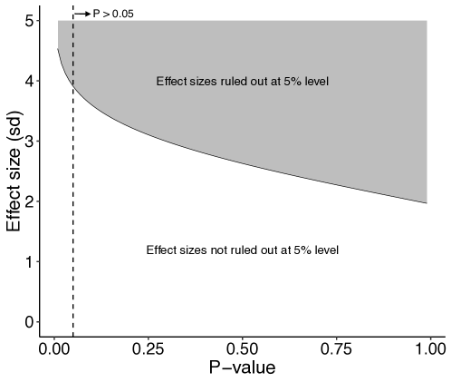
Figure 1: Effect size vs. p-value. The x-axis denotes the p-value obtained in a conventional 2-sided z-test, and the y-axis denotes the absolute value of the effect size, measured in standard deviations. The dotted line indicates the traditional cutoff of p = 0.05. The gray region indicates effect sizes ruled out at the 5% level by a non-inferiority test given the corresponding p-value on the x-axis. The white region indicates effect sizes consistent with the corresponding x-axis p-value at the 5% level.

2.4.2 Confidence intervals

With a confidence interval from a traditional test, we can also assess the range of values that can be ruled out at the 5% level. Suppose a researcher performs non-inferiority tests over a range of thresholds (e.g., Figure 2). There is always some $\delta$ sufficiently large that $p<0.05$; this is approximately $\delta=0.7$ in Figure 2. This $\delta$ where the p-value crosses $0.05$, the smallest effect that can be ruled out with a $5\%$ error rate, is equivalent to the upper bound on the one-sided 95% confidence interval for $\theta$. To understand this relationship between non-inferiority testing and the confidence interval, recall the link between confidence intervals and hypothesis tests: we reject the null hypothesis of no effect at the $\alpha$ level if 0 does not lie in the $1-\alpha$ confidence interval. The same relationship holds for other null hypotheses, and confidence intervals can be made by inverting test statistics.

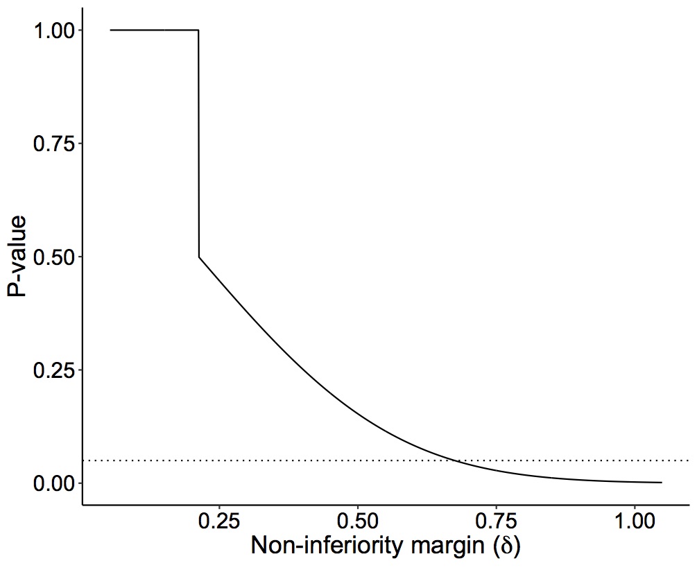
Figure 2: Non-inferiority plot. The x-axis indicates the non-inferiority margin, and the y-axis the p-value. The dotted horizontal line indicates p = 0.05. The solid line corresponds to the p-value associated with a test that the effect is less than the corresponding non-inferiority margin. Generated from simulated data.

2.4.3 Recommendations

If researchers know a non-inferiority threshold, they can run a non-inferiority test. When a threshold is difficult to define, they can instead present the confidence interval in a non-inferiority framework. For example, researchers might avoid statements like, “We find no evidence of an effect (p = 0.6, 95% CI: -1.4 to 2.6)” or “The effect is statistically insignificant and small.” Instead, they can say, “We can rule out effects less than -1.4 and greater than 2.6 at the $\alpha=0.05$ level,” and interpret the magnitude of these effects in the context of the problem. Researchers can also select different values of $\alpha$, e.g., $\alpha=0.1$ for a narrower interval, based on the importance of the assumption under evaluation.

3 Threshold selection and power

These recommendations leave unresolved the question of how to select a reasonable threshold. Researchers want violations to be as small as possible. Ideally, a researcher could rule out all violations that are meaningful in the context of the problem, whether by selecting a specific threshold or by examining the bounds of the confidence interval of the violation. However, researchers may be limited by a lack of power. In this section, we discuss the power of tests that examine a violation parameter that is measured on the scale of the treatment effect and use this to inform threshold recommendations.

3.1 Non-inferiority power heuristic

Proposition 3 (Non-inferiority power heuristic)

If a one-sided test has probability $1-\beta$ of detecting $\theta=\theta^{*}$ (given such an effect exists) at the $1-\alpha$ level, then the non-inferiority formulation will have probability approximately $1-\beta$ of ruling out $\theta\geq\theta^{*}$ (given no violation exists). (A derivation is provided in Appendix D, with additional discussion in Appendices E and F.)

This heuristic informs us that when an assumption is met (i.e., no violation), our power to rule out a violation as big as the treatment effect for which our main analysis is powered is approximately the same as the power of the main analysis. Put another way, if the main study is just powered for all treatment effects of practical significance, tests of assumptions will be just powered to detect violations of that magnitude.

While this heuristic appears to suggest that a well-powered study is well-powered to examine assumptions, in truth, we low power in many cases. First, tests of model assumptions may guide whether an analysis should be performed. Therefore, researchers may need to pass both the model assumption test and the main treatment effect test to report a positive result. Even if researchers were only interested in ruling out violations of the same magnitude as the treatment effect the main study is powered to detect, there is a lower probability of passing both the model assumption test and the treatment effect test.

If the power of the main study is low, this heuristic tells us that the power of tests of model assumptions will also be low. Still, even if a study is well-powered, tests of model assumptions often have low power. For instance, researchers may perform a placebo test on a portion of the sample. Likewise, researchers exclude data from after the start of the intervention to perform a parallel trends test.

A non-inferiority test will also have lower power to rule out a violation smaller than the treatment effect of interest. For example, in Figure 3, we display the power to rule out a range of violations. Suppose the main study has $80\%$ power to detect an effect of $\theta=\delta$. As the top line shows, there is $80\%$ power to rule out violations greater than or equal to $\delta$ if there is truly no effect ($\theta=0$). However, if were are interested in smaller violations, we have much less power. For example, we have only $31\%$ power to rule out a violation $\geq 0.5\delta$ when $\theta=0$. In the context of the parallel trends test, this would suggest we have low power to rule out violations that might account for half of our treatment effect, even if the study is well-powered.

In addition, a violation may be small but still greater than 0. Suppose our main study has $80\%$ power to detect an effect of size $\delta$. We have $80\%$ power to rule out this violation if it is truly 0, the peak of the top line in Figure 3. As the true violation increases, power decreases, corresponding to the different lines in Figure 3. For example, if there is a true violation of $\theta=0.5\delta$, we have only $25\%$ power to rule out a violation of size $\delta$. Even if the true violation size is not practically significant, it will nevertheless reduce power to rule out large violations.

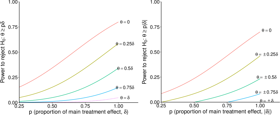
Figure 3: Non-inferiority power. The left panel refers to a one-sided test and the right panel to a two-sided test. The x-axis indicates the value of p in the null hypotheses, $\theta\geq p\delta$ and $\theta\geq p|\delta|$ respectively. The y-axis indicates the power to reject this null, with each line indicating a different true effect size. Maximum power is achieved when $\theta=0$, and power decreases as $\theta$, the size of the violation, increases. The solid lines show power to reject in cases in which the null hypothesis is not true; the dotted line refers to the case when $\theta=\delta$, thus falling under the null hypothesis.

3.2 Threshold selection

In general, researchers should select thresholds that are grounded in their research context. They should also consider the treatment effect for which the main study was powered as an upper bound on $\delta$. If authors performed a pre-specified power analysis, the minimum detectable effect (MDE) can be used to set this threshold. If a pre-specified analysis is not available, some authors have proposed using randomization inference on observed data to estimate the MDE (e.g., Black et al. (2019)).

It may be tempting to use estimated coefficients and standard errors to understand a study’s power. By this logic, researchers would use the observed distribution to estimate the probability that a coefficient drawn from that distribution would be statistically significant. However, this “empirical power” is a misleading transformation of the p-value (Levine and Ensom, 2001; Gelman, 2019). (See Appendix H for further details.) A related approach could involve subtracting off the treatment effect of interest, then adding in a pre-specified violation, and estimating power, but this has similar limitations (Hoenig and Heisey, 2001).

If authors use the estimated treatment effect as the chosen non-inferiority threshold without additional analysis, they will not know the study’s expected power to rule out an effect of this magnitude. However, this would most likely be a relatively generous threshold for the test, as evidence suggests that treatment effects are often inflated due to publication bias (Ioannidis et al., 2017).

4 Difference in differences and parallel trends

We next consider in greater detail applying these principles to testing the parallel trends assumption in DID. The parallel trends assumption as currently implemented serves two functions. First, it is reflected in the estimation strategy, setting the trend difference between treatment and comparison groups equal to 0. Second, observing parallel trends in the pre-intervention period provides evidence that the relationship between treatment and comparison groups is sufficiently smooth that it can be extrapolated into the post-intervention period. Researchers use the comparison group to impute the counterfactual for the treatment group in the post-intervention period. They want to trust that there is a stable relationship between the two groups and that any shocks would have impacted the two groups similarly. If the groups appear to be on very different trajectories, this seems less plausible.

We separate these two aspects of parallel trends. We argue that researchers should include a differential trend in the base model for the same reason that they model level differences between units: it would introduce bias to incorrectly assume that groups have the exact same value, and we typically do not think that small differences would change the validity of our counterfactual. Even if a trend difference is small, forcing this parameter to be exactly 0 introduces bias. Nevertheless, researchers should provide evidence that trends are fairly stable, close enough to parallel, that we trust DID’s extrapolation into the post-intervention period. This entails providing evidence that trend differences between treatment and comparison groups are small enough to have a negligible impact on the treatment effect. If this is not the case, researchers should then provide statistical evidence that trend differences are sufficiently close to a different stable data-generating process, such as parallel paths.

4.1 “One step up” approach

Applying a non-inferiority framework, researchers can examine evidence that differential trends between treatment and comparison groups would meaningfully impact the treatment effect estimate. They involves ruling out large trend differences between treatment and comparison groups. To implement this, we propose a “one step up” approach:

1. Specify a base model that includes a linear trend difference ($+\beta td_{i}$) (Eq. 2). This is often the specification used in a parallel trends test, including post-intervention data.

2. Compare the treatment effect in the base specification to the treatment effect in a specification without a trend difference (Eq. 1). Conclude one of the following:

   1. Unclear evidence: If there is a wide confidence interval on the difference in treatment effects that includes $\delta$, conclude that there is weak evidence to evaluate the parallel trends assumption. Authors cannot provide statistical evidence about the strength of this assumption.

   2. Strong evidence of no change: If authors can rule out differences greater than $\delta$, conclude that parallel trends holds. Consider doing sensitivity analysis with a more complex model (e.g., spline trend difference).

   3. Strong evidence of change: If treatment effects and their difference are precisely estimated but we cannot rule out differences of at least $\delta$, proceed to (3) if the parallel growth assumption seems reasonable in study context.

3. If trends are not parallel, use a more complex trend difference, such as a spline, in the baseline model and compare to the linear specification. Use the procedure in (2) to determine the strength of evidence for this model. If tests are applied sequentially, a correction for multiple testing should be used.

4.2 Justification and trade-offs

Our approach calls for reporting the baseline treatment effect from a model with a linear trend difference. If there is no violation, this model is still unbiased, but reduces power to detect a treatment effect compared to the conventional model that assumes no trend difference. However, we believe that power to evaluate the treatment effect in a model that includes a trend difference is key to DID. Whenever we lack power to detect a treatment effect in a more complex model, we also lack power to detect meaningful violations of parallel trends. Forcing the trend difference to be 0 increases power but overstates our confidence in our model assumption. Likewise, if we do not believe that trends are parallel and want to model linear trend differences between treatment and comparison groups, we need to show evidence against more complex trend differences.

As trend differences become more complex, the power to detect an effect decreases.

Proposition 4 (Trend difference impact on standard error)

When we add a trend difference into Eq. (1), creating Eq. (2), if there is no violation of parallel trends, the standard error on our treatment effect in the expanded model $\beta_{1j}$ relates to the standard error of our treatment effect in the original model, $\beta_{1k}^{\prime}$:

$$\frac{{\sigma}^{2}_{\beta_{1j}}}{{\sigma}^{2}_{\beta_{1k}^{\prime}}}\geq 1-\frac{R^{2}_{\mathbb{I}(T=k\cap D=1)|DT}}{1-R^{2}_{\mathbb{I}(T=k\cap D=1)|X_{-k}}}$$ (11)

where $R^{2}_{\mathbb{I}(T=k\cap D=1)|X_{-k}}$ is the coefficient of determination when $\mathbb{I}(T=k\cap D=1)$ is regressed on all other variables in the reduced model and where $R^{2}_{DT|\mathbb{I}(T=k\cap D=1)}$ is the coefficient of determination when $d_{i}t_{i}$ is regressed on $\mathbb{I}(t=k\cap d_{i}=1)$. This relationship similarly applies to other trend differences, e.g., replace $d_{i}t_{i}$ with $d_{i}t_{i}^{2}$. See Appendix G for proof.

If there is no violation, adding a trend difference will increase the standard error of our treatment effect. The term in the numerator tells us that holding all other parameters fixed, the decrease in power will be smaller when the length of the pre-intervention time series is different than the length of the post-intervention time series. Power decreases more sharply when the two are nearly equal. However, models with a greater number of time points will generally have higher power initially, making an increase in standard error less consequential.

The decrease in power will also be more substantial in models with pre-existing correlated covariates, per the term in the denominator. For example, when adding a linear trend difference, standard error increases somewhat. By contrast, as we move from linear to quadratic trend difference, there is a much greater decrease in power, rendering it often impractical to use the latter. Overall, a baseline linear trend difference model reduces bias and detects many violations of parallel trends while also maintaining reasonable power to detect a treatment effect when there is no violation.

4.2.1 Simulations

We illustrate this trade-off more concretely with simulations, using parameters from Table 3. In the “none” type, we assume the data-generating process from Eq. (1), with $\epsilon_{i}\sim N(0,1)$. In the “linear” type, there is a linear trend difference between treatment and comparison groups. In the “midpoint change” type, a linear trend difference of the same slope begins after the midpoint of the pre-intervention time period. In the “last pre-period jump” type, the treatment effect begins in the last pre-intervention period.

Number of treatment groups	{5,10,50}
Number of comparison groups	{10,50,100}
Number of pre-intervention periods	{5,15}
Number of post intervention periods	{5, 15}
Violation types	{None, last pre-period jump, linear, midpoint change}
Treatment effects (sd)	{.5, 1}

Table 3: Simulation parameters.

For each scenario, we run 500 trials. We fit 6 models each time: no trend difference, linear, quadratic, cubic, a restricted cubic splines with 2 degrees of freedom (knot placed at the median), and a generalized additive model (GAM) with penalty selected by generalized cross-validation.

4.2.2 Power decreases as trend differences become more complex.

Figure 4 shows that when there is no violation of parallel trends, power declines as the modeled trend difference becomes more complex. This decline is steeper when there are fewer treated groups or pre-intervention periods or when the treatment effect is smaller. It is also steeper when there are more post-intervention periods as trend differences become more extreme when extrapolated over a long time horizon. Even in situations with extremely high power to detect an effect in a model with no trend difference, quadratic and cubic trend differences often reduce power to an impractical extent, and we do not recommend these models.

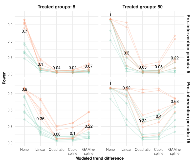
Figure 4: Power across different scenarios (no violation). We show the power to detect an effect when there is no trend violation using the trend difference model on the x-axis. Across the rows, we vary the number of treated groups, and across the columns the number of pre-intervention periods. Color indicates treatment effect size: orange is 1 standard deviation, and green is 0.5 standard deviations. Median power across different scenarios (trials = 200 per scenario) is labeled.

4.2.3 We have similar power to detect treatment effects as we do to rule out changes in treatment effects across models.

In Figure 5, we consider the heuristic described in the previous section. We observe that we have approximately equal power to rule out a violation the size of our treatment effect as we do to detect the treatment effect in the model with a trend difference. (All of these tests control the rate of false positive results at the 5% level.) This relationship can inform our threshold selection, as previously discussed. It also underscores the value of moving to a more complex model as baseline, as insufficient power to detect an effect in a model with a trend difference may also suggest insufficient power to rule out meaningful violations of parallel trends.

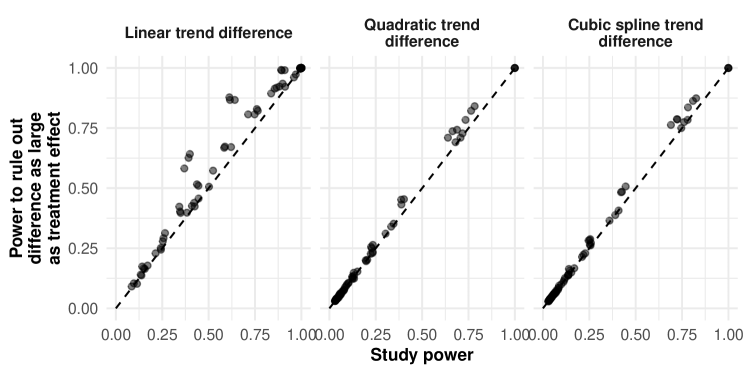
Figure 5: Power to rule out differences in treatment effect across different models. In these scenarios, there is no violation of parallel trends. The x-axis shows the power to detect the treatment effect using the model in the plot title. The y-axis shows the power to rule out a change this size between estimated treatment effects in that model and a model with no trend difference. Each point represents estimates from one of simulation scenarios (trials = 200). Within each boxplot, there is variation in number of treatment and comparison groups as well as number of post-intervention periods.

4.2.4 Modeling complex trend differences can reduce bias but may increase mean-squared error.

In Figure 6, we illustrate how complex models can reduce bias. Even when linear trend differences cannot completely eliminate bias due to a more complex data-generating process like a midpoint trend change, they can still help detect non-parallel trends without increasing bias, even in short time series. The GAM that is penalized to reduce overfitting can reduce bias when there is a sufficient number of pre-intervention time points. This may be helpful when, for example, there is a long pre-intervention time series, and we want to extrapolate the observed trend difference close to the time of the intervention.

Splines allow more curvature in the trend, but the more local fitting of these models also raises a conceptual question: if trend differences are not stable over the pre-intervention time period, should we feel comfortable extrapolating over the post-intervention time period? For example, if trends are not parallel until shortly before an intervention begins, we may not trust that they would remain parallel in the post-intervention period. For this reason, we might assess both a linear and spline model, but would not use only the latter. Third, none of our models could address a jump during the last pre-intervention period, and therefore, other methods should be used to consider this type of parallel trends violation.

Our choice of a linear model as baseline is also informed by results in Figure 7: even in the “Midpoint change” scenario in which the GAM reduces bias compared to the linear model, mean-squared error nevertheless exceeded the linear trend difference in every scenario we considered, particularly when there was a long post-intervention period.

Overall, these simulations underscore the conceptual justification above: a “one up step approach” more closely aligns power to detect a treatment effect with study power, reduces bias, and is more explicit about the type of parallel trends violations we can rule out.

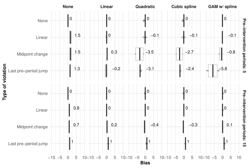
Figure 6: Bias across different scenarios. Each column indicates a different modeled trend difference. In the top row, we show scenarios with 5 pre-intervention periods, and in the bottom row with 15 pre-intervention periods. The y-axis shows the true underlying data-generating process. Average bias per scenario (trials = 500) is plotted on the x-axis, with the median labeled in text.

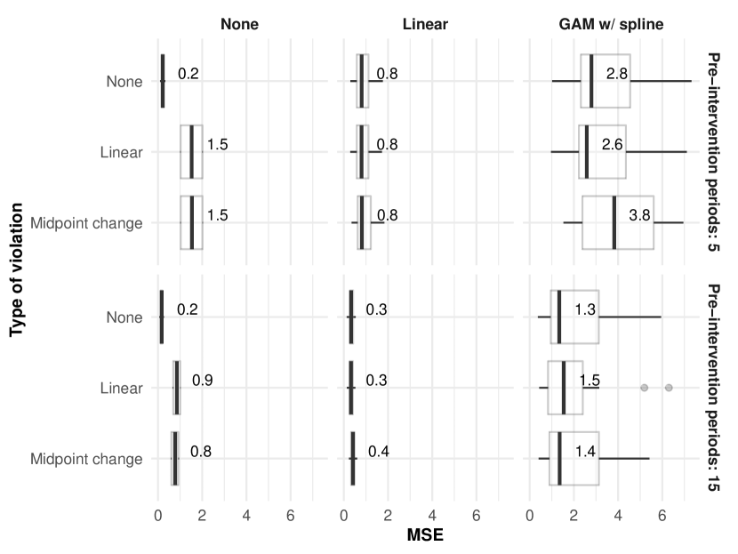
Figure 7: Mean-squared error across different scenarios. Each column indicates a different modeled trend difference. In the top row, we show scenarios with 5 pre-intervention periods, and in the bottom row with 15 pre-intervention periods. The y-axis shows the true underlying data-generating process. Average bias per scenario (trials = 500) is plotted on the x-axis, with the median labeled in text.

5 Re-analysis of the impact of Affordable Care Act on dependent coverage

We apply this approach to analyzing the impact of the 2010 Patient Protection and Affordable Care Act (ACA) on dependent coverage. The ACA was passed on March 23, 2010. Beginning on September 23, 2010, it required that commercial insurers offer coverage to dependents on a parent or guardian’s plan until age 26. Several papers have assessed the impact of this provision using a DID model, comparing coverage among those newly eligible to join parents’ plans (aged 18-25) with those who were not in the relevant age window (either below 18 or over age 25) (Akosa Antwi et al., 2013; Barbaresco et al., 2015; Sommers et al., 2013; Cantor et al., 2012). These papers identified strong impacts on dependent coverage and were widely covered in the media and cited in the academic literature (Kohn, 2015; Tavernise, 2012).

We focused on the ACA dependent coverage provision for a few reasons. First, there was a simple, mechanical link between the intervention and outcome (i.e., a coverage expansion should provide more coverage). Second, several large, open-source data sets measured the outcome of interest, allowing us to compare findings across different well-powered analyses. In addition code for one paper was open-source (Akosa Antwi et al., 2013). Rather than critique these studies, we use these examples to explore the complexity of the issues we raise.

We re-analyzed these studies and assessed changes in estimated treatment effect under different trend assumptions. We first show that in one data set, allowing for a trend difference markedly reduced treatment effects, which occurred despite authors having tested for the significance of the trend term and finding an insignificant result. We investigate this further and find that some of the trend difference may have been driven by state dependent coverage laws that existed prior to the ACA. We next compare the impact of allowing more flexible trend differences in other datasets. While effects are more stable in these papers, we show that differential trends often lead to smaller treatment effects when the pre-intervention period begins after 2008.

5.1 Reanalysis of Akosa Antwi et al. (2013)

5.1.1 Background

We used public replication code provided by Akosa Antwi et al. (2013) to re-analyze their results. The authors used data from the nationally representative Survey of Income and Program Participation (SIPP). They compared people aged 19-25 to those 16-18 and 27-29. As their primary result, they reported significant effects on insurance coverage, driven by increases in rates of dependent coverage.

To assess the assumption of parallel trends, the authors tested whether there was a difference in linear trend between treatment and comparison groups and found no statistically significant result (original paper Appendix Table A1). They also visually inspected the trend in proportion insured, noting that it was was fairly stable until ACA passage (original paper Figure 1).

5.1.2 Methods

We first modified the authors’ specification to include a treatment effect measured at each post-intervention time point to ensure that we would only identify the trend difference from pre-intervention data (see footnote 3 in this paper):

$$Y_{igst} =\alpha+\gamma Treat_{g}+\sum_{\ell=10/2010}^{11/2011}\delta_{\ell}Implement_{t}+\sum_{k=3/2010}^{9/2010}\mu_{k}Enact_{t}+$$

$$\sum_{\ell=10/2010}^{11/2011}\eta_{\ell}\left(Treat_{g}\times Implement_{t}\right)+\sum_{k=3/2010}^{9/2010}\sigma_{k}\left(Treat_{g}\times Enact_{t}\right)+$$

$$\mathbf{X}_{igst}\mathbf{\beta}+\tau_{t}+\xi_{s}+\epsilon_{igst},$$

where $Y_{igst}$ was a binary variable equal to 1 if person $i$ in age range $g$ and state $s$ at time $t$ had the insurance type and 0 otherwise, $\mathbf{X}_{igst}$ represented individual-level factors, $Implement_{t}$ is a dummy variable equal to 1 post-implementation and 0 otherwise and $Enact_{t}$ is equal to 1 post-enactment but prior to implementation and 0 otherwise, and $Treat_{g}$ represented being in the 19-25 age range.

We then considered 2 modifications:

1. Linear trend difference ($+\pi Treat_{g}t$:) We allowed for a linear trend difference between treatment and comparison groups.

2. Spline trend difference ($+f(\pi Treat_{g}t)$): We used the GAM package in R to allow a penalized cubic regression spline trend difference. Penalization was chosen with generalized cross-validation.

There were 20 pre-intervention time points for fitting these trends. While the original paper considered both enactment and implementation effects, we focused on the latter, i.e. $\eta=\frac{1}{14}\sum_{\ell=10/2010}^{11/2011}\eta_{\ell}$. Following the authors, we used White robust standard errors, clustered at the state level for our models. We used randomization inference at the age level to test the difference in treatment effects between models. We note whether we can rule out differences in treatment effects of 2%, our selected substantive threshold, and the size of the treatment effect.

To break down results by states with prior dependent coverage, we used data from the National Council of State Legislatures to identify states with dependent coverage and WestLaw to identify when coverage came into effect (Dependent Health Coverage and Age for Healthcare Benefits, n.d.). We determined whether survery respondents were eligible for dependent coverage based on age, student status, and marital status.

5.1.3 Results

In Figure 8, we show the impact of including differential trends on insurance coverage treatment effects. For nearly all results, the point estimate fell substantially, and all statistically significant results became insignificant. We also provide event-study plots for the 2 outcomes for which the authors performed parallel trends tests: whether adults aged 19-25 had any insurance, and whether they had coverage as a dependent (Figure 9).

In Table 4, we provide further details. For the model fit to any health insurance, the treatment effect fell from 3.2% to 1% with the linear trend difference. The GAM had a slightly higher point estimate, but the confidence interval was extremely wide (4%, 95% CI: -0.04 to 0.12). In the event study plot, we observe a slight upward trend prior to the passage of the ACA. This trend may have leveled out during 2009, but given the short time series, it is difficult to know whether this can be extrapolated into the post-intervention time period.

The change in treatment effects for dependent coverage was more substantial. The dependent coverage estimates decreased from 7% to 2% when a linear trend difference was added, with a similar result in the GAM model. In the event-study plot we observe a clear upward trend.

Overall, we could not rule out a 2% change in treatment effect between the no trend difference and linear trend difference models for any outcomes except for government insurance coverage. This, along with the substantial and statistically significant changes we see in treatment effects, provided evidence against parallel trends. However, we could rule out 2% changes in treatment effects between models with linear and spline trend differences for dependent coverage, individual coverage, and employer coverage, which suggested that differential trends may be fairly linear in this data.

To consider one explanation for the observed non-parallel trends, we re-analyzed results estimating different treatment effects for those who were not covered by a dependent coverage law prior to the ACA (Figure 10) and those who were (Figure 11). In these results, we saw far less of an impact of differential trends for the group that was not covered by prior laws, with generally stable treatment effects. We could rule out changes of more than 2% in treatment effects between models with no trend difference and a linear trend difference. By contrast, in the group covered by prior laws, we saw a substantial and statistically significant impact of pre-intervention trends, particularly for dependent and employer coverage. These results suggest that we may estimate a smaller impact of ACA dependent coverage expansion if we account for differential trends, particularly among individuals covered by a prior law.

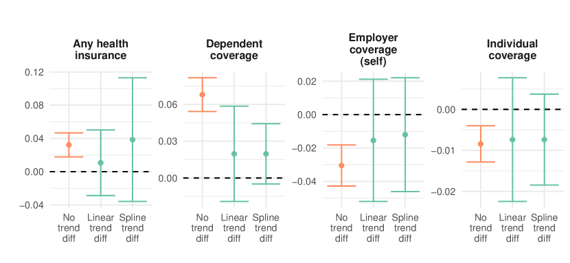
Figure 8: Treatment effects. The panel shows estimated treatment effects across models. The orange points are statistically significant at the 5% level; green points are not.

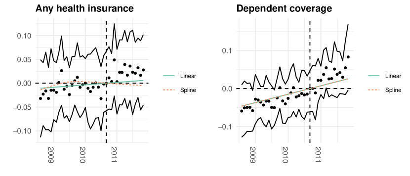
Figure 9: Event study plots. For each time point, we estimated the treatment effect compared to the third quarter of 2010, the last quarter before the ACA was implemented.

Outcome	Model	Treatment effect	Difference (vs. simpler model)	CI of difference	Rule out 2% change	Rule out tx effect
Any health insurance	No trend difference	0.03 (0.01)***
Any health insurance	Linear trend difference	0.01 (0.02)	0.02	(0.006, 0.04)	No	No
Any health insurance	Spline trend difference	0.04 (0.04)	-0.028	(-0.029, -0.027)	No	Yes
Dependent coverage	No trend difference	0.07 (0.01)***
Dependent coverage	Linear trend difference	0.02 (0.02)	0.05	(0.02, 0.08)	No	No
Dependent coverage	Spline trend difference	0.02 (0.01)	$\sim$0	(-0.001, 0.001)	Yes	Yes
Individual coverage	No trend difference	-0.01 (0)***
Individual coverage	Linear trend difference	-0.01 (0.01)	$\sim$0	(-0.01, 0.003)	Yes	No
Individual coverage	Spline trend difference	-0.01 (0.01)	$\sim$0	(-0.0004, 0.0004)	Yes	No
Employer coverage (self)	No trend difference	-0.03 (0.01)***
Employer coverage (self)	Linear trend difference	-0.015 (0.02)	-0.02	(-0.03, -0.0002)	No	No
Employer coverage (self)	Spline trend difference	-0.012 (0.02)	-0.003	(-0.004, -0.003)	Yes	Yes
Government insurance	No trend difference	$\sim$0 (0.01)
Government insurance	Linear trend difference	0.01 (0.01)	-0.01	(-0.013, -0.01)	Yes	No

Table 4: Model results. Model indicates the model for the trend difference. The difference column indicates the difference in treatment effect between the model and the simpler model above. The last two columns assess the magnitude of this difference: whether we can rule out a difference of 2% and a difference the magnitude of the treatment effect. *$p<0.1$, **$p<0.05$, ***$p<0.01$

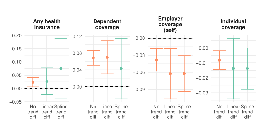
Figure 10: Treatment effects (no prior dependent coverage law). For these treatment effects, the treatment group includes only individuals not covered by a prior law. The panel shows estimated treatment effects across models. The orange points are statistically significant at the 5% level; green points are not.

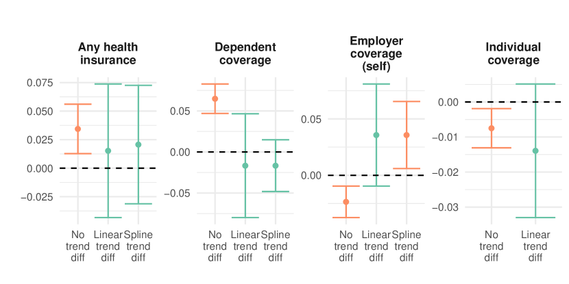
Figure 11: Treatment effects (with prior dependent coverage law) This panel only includes a treatment group covered by a previous law. The panel shows estimated treatment effects across models. The orange points are statistically significant at the 5% level; green points are not.

5.2 Comparison to other papers

We compared these results to those of 3 other papers, which used different nationally representative surveys in their estimates. We outline characteristics of the different papers in Table 5. These papers estimated much larger effects than Akosa Antwi et al. (2013) and used slightly different treatment and comparison groups and time horizons. Barbaresco et al. (2015) used data from 2007 to 2013 and compared only 23-25-year-olds to 27-29-year-olds, citing concerns about demographic differences between groups. Sommers et al. (2013) used data from 2005 to 2011 and compared ages 19-25 to 26-34. Cantor et al. (2012) used data from 2004 to 2010 and compared ages 19-25 to 27-30.

We report re-analyses for these papers in Table 6. We generally observed small shifts in point estimates for treatment effects across different trend difference models. We were unable to rule out differences greater than 2% for nearly all models, but were generally able to rule out differences the size of our treatment effects.

We also re-analyzed using strategies more similar to those in the first paper. In a next analysis, we matched the timeline, comparison group, and control variables as closely as possible to Akosa Antwi et al. (2013) (Table 7). We see a greater impact of including differential trends. In particular, the BRFSS estimate declined from 5% to 2.8% for the any health insurance coverage outcome and the CPS estimate for dependent coverage declined from 5% to 2% when linear trends were included. Likewise, the point estimate decreased substantially for those covered by a prior dependent coverage law but remained stable for those who were not.

	Akosa Antwi, Moriya, and Simon	Barbaresco, Courtemache, and Qi	Sommers, Buchmueller, Decker, Carey, and Kronick	Cantor, Monheit, DeLia and Lloyd
Journal	American Economic Journal: Economic Policy	Journal of Health Economics	Health Affairs	Health Services Research
Year	2013	2015	2013	2012
Data source	Survey of Income and Program Participation	Behavioral Risk Factor Surveillance System	Replicated National Health Insurance Survey (NHIS) section	Current Population Survey
Code publicly available	Yes	No	No	No
Years analyzed	2008-2011	2017-2013	2005-2011	2014-2010
Treatment ages	19-25	23-25	19-25	19-25
Comparison ages	16-18, 27-29	27-29	26-34	27-30
Effects measured	Any insurance, type of insurance, labor force outcomes	Insurance, PCP, other health outcomes	Any insurance, private insurance	Any insurance, dependent coverage
Visual plot	Yes, without CI	Yes, with CI	Yes, without CI	No
Event-study plot	No	No	No	No
Test for difference in trends	Yes	No	Yes	Yes
Different follow-up times	No	Yes	No	Yes
Adjust for previous coverage	No	Yes (control variable)	No	Yes
Estimated effect	3%	7%	7%	5%

Table 5: Comparison of dependent coverage papers.

Data set	Outcome	Model	Treatment effect	Difference (vs. simpler model)	CI of difference	Rule out 2% change	Rule out tx effect
BRFSS	Any health insurance	No trend	0.059 (0.016)**
BRFSS	Any health insurance	Linear trend	0.044 (0.014)**	-0.015	(-0.04, 0.01)	No	Yes
BRFSS	Any health insurance	Spline	0.065 (0.026)**	0.02	(0.015, 0.03)	No	Yes
NHIS	Any health insurance	No trend	0.052 (0.008)***
NHIS	Any health insurance	Linear trend	0.046 (0.012)***	0.007	(-0.02, 0.01)	No	Yes
NHIS	Any health insurance	Spline	0.046 (0.009)***	$\sim$0	(-0.01, 0.01)	Yes	Yes
CPS	Any health insurance	No trend	0.042 (0.01)***
CPS	Any health insurance	Linear trend	0.039 (0.01)***	0.003	(-0.013, 0.018)	No	Yes
CPS	Dependent coverage	Linear trend	0.042 (0.006)***
CPS	Dependent coverage	No trend	0.037 (0.005)***	0.005	(-0.013, 0.003)	No	Yes

Table 6: Comparisons across papers. Model indicates the model for the trend difference. The difference column indicates the difference in treatment effect between the model and the simpler model above. The last two columns assess the magnitude of this difference: whether we can rule out a difference of 2% and a difference the magnitude of the treatment effect. *$p<0.1$, **$p<0.05$, ***$p<0.01$

Data set	Outcome	Model	Treatment effect	Difference (vs. simpler model)	CI of difference	Rule out 2% change	Rule out tx effect	Treatment effect without prior law	Treatment effect with prior law
BRFSS	Any health insurance	No trend	0.05 (0.01)***	0				0.04 (0.01)**	0.06 (0.02)**
BRFSS	Any health insurance	Linear trend	0.03 (0.05)	0.03	(-0.004, 0.06)	No	No	0.07 (0.04)	-0.003 (0.07)
BRFSS	Any health insurance	Spline trend	-0.04 (0.87)	0.06	(0.06, 0.07)	No	No	0.13 (0.09)	-0.13 (0.99)
CPS	Any health insurance	No trend	0.04 (0.01)***	0				0.04 (0.01)***	0.05 (0.01)***
CPS	Any health insurance	Linear trend	0.05 (0.02)**	-0.01	(-0.02, 0.001)	No	No	0.08 (0.03)***	0.02 (0.03)
CPS	Dependent coverage	No trend	0.05 (0.01)***	0				0.05 (0.01)***	0.06 (0.01)***
CPS	Dependent coverage	Linear trend	0.02 (0.02)	0.03	(0.02, 0.04)	Yes	Yes	0.04 (0.02)**	0.003 (0.02)

Table 7: Comparisons across papers (sample matched to Akosa Antwi et al. (2013) as closely as possible). Model indicates the model for the trend difference. The difference column indicates the difference in treatment effect between the model and the simpler model above. The last two columns assess the magnitude of this difference: whether we can rule out a difference of 2% and a difference the magnitude of the treatment effect. *$p<0.1$, **$p<0.05$, ***$p<0.01$

5.3 Reconciling interpretations

There are several potential interpretations for the different results across papers and over time.

1. Power: First, the change in trends in 2008 might be random noise. When we truncate the dataset later years, we reduce power, and we may be underpowered to fit complex trends. However, even when truncating the data to late 2008, in the SIPP and BRFSS datasets, we have 15 pre-intervention time points, which our simulations suggested was an appropriate length for this type of analysis.

2. Conceptual noise: Even if trends diverged in late 2008, this fact may be unimportant for questions of interest. The overall stability of trends prior this may suggest that the comparison groups were generally on parallel paths.

3. Accumulation of small differences: Extrapolating the trend difference into the post-period may magnify unimportant differences. When the post-intervention period is long, even a small difference can have a large impact on the estimated treatment effect.

Nevertheless, this trend change may also reflect a meaningful development.

1. Financial crisis: Age groups may have diverged from one another during the financial crisis as a result of trends in the labor market, and it is unclear whether they would have returned by the time of the provision’s implementation.

2. Pre-ACA dependent coverage: Thirty-seven states had implemented some form of dependent coverage prior to the ACA, covering about 50% of individuals (although a lower proportion had parents in plans that could take advantage of these laws). Our analysis suggests that some of the observed difference in trends might have been driven by differences between these groups.

Overall, our analysis of dependent coverage highlights several considerations for a non-inferiority approach to parallel trends testing. In particular, when applying our “one step up approach”, it may be useful to explore whether trends are roughly parallel in a range of outcomes, to consider the most appropriate time horizon, and to model potential drivers of differential trends. As previous papers have argued, contextual reasoning for why trends are likely to be parallel can help in thinking through the validity of the parallel trends assumption (Kahn-Lang and Lang, 2018), and this can be combined with our modeling approach to inform analysis of trends.

6 Conclusion

Many tests of model assumptions incorrectly assume a null hypothesis of “no violation.” We provide estimators for conducting non-inferiority versions of these tests and explore their power. We also provide conceptual and statistical guidance for undertaking this process in the case of the parallel trends test with the “one step up” approach: calling for researchers to present base results from a model with a trend difference and assess the difference from a simpler model when validating parallel trends. We show that this approach reduces bias and sets a more reasonable standard for the power needed to assess parallel trends. We use this to demonstrate that several papers analyzing the impact of the dependent coverage mandate of the ACA may have had less robust evidence for an effect than previously considered. Future work may consider alternative types of trend differences and how to select the most appropriate pre-intervention time series length in DID. It may also consider how to combine our approach with other quasi-experimental estimators including matching and synthetic controls as well as developing estimators for other non-inferiority tests. Overall, using a non-inferiority approach, we can better assess the strength of evidence for model assumptions.

Appendix A Search terms Google Scholar results in Table 1

In Table 8, we present the search results used to obtain results in Table 1. Searches were conducted on May 6, 2018. These are imprecise metrics for several reasons. Some unrelated articles may be included in results, and some tests required more specific search terms than others. (For example, we did not search “Komogorov-Smirnov” without “test” because that term also applies to some theorems. However, we searched “Dickey-Fuller” because to our knowledge this only commonly applies to the corresponding test.) In Table 9, we provide an expanded version of Table 1 that includes breakdown by journal as well as all Google Scholar results.

To limit our results to those from a particular journal, we used the following search criteria:

• Quarterly Journal of Economics: site:academic.oup.org/QJE

• American Economic Review: source:“American Economic Review” AND site:aeaweb.org

• Econometrica: source:“Econometrica”

• Journal of Political Economy: source:“Journal of Political Economy” AND site:journals.uchicago.edu

• Review of Economic Studies: source:“Review of Economic Studies” AND site:academic.oup.com

• Journal of Finance: source:“The Journal of Finance” AND site:onlinelibrary.wiley.com

Test	Google Scholar search term
Parallel trends test	“parallel trends test” OR “parallel trends assumption” OR “test of parallel trends” OR “assumption of parallel trends” OR “difference-in-differences” OR “event study”
Placebo test	“placebo test” OR “placebo tests”
Kolmogorov-Smirnov test	“kolmogorov-smirnov test”
Balance tests	(“balance test” OR “balance tests” OR “balance table”) [AND “experiment” when searching outside of econ journals]
Durbin-Wu-Hausman test	“Durbin-Wu-Hausman test” OR “Hausman test”
Dickey-Fuller (DF)/ Augmented DF	“Dickey-Fuller” OR “Augmented Dickey-Fuller”
Sargan-Hansen test	“Sargan-Hansen test” OR “hansen test” OR “Sargan test”
McCrary test	“mccrary test” OR “mccrary tests”
Proportional hazards test	“proportional hazards” OR “proportional hazards test” OR “proportional hazards assumption” OR “test of proportional hazards” OR “assumption of proportional hazards”
Levene, Bartlett, White/Breusch-Pagan tests	“Levene test” OR “Bartlett test” OR “Breusch-Pagan test” OR “Levene’s test” OR “Bartlett’s test” OR “Breusch-Pagan’s test” OR “White’s test”
Shapiro-Wilk, Anderson-Darling, Jacque-Bera tests	“Shapiro-Wilk” test OR “Anderson-Darling test” OR “Jarque-Bera test” OR “Shapiro-Wilk’s test” OR “Anderson-Darling’s test” OR “Jarque-Bera’s test”
Hosmer-Lemeshow test	“hosmer lemeshow”

Table 8: Google Scholar search terms for Table 1

Test	Quarterly Journal of Economics	AER	Econometrica	Journal of Political Economy	Review of Economic Studies	Journal of Finance	Economics total	Google Scholar total
Parallel trends test	21	44	128	16	23	61	293	17,600
Placebo test	15	21	54	8	10	35	143	9,110
Kolmogorov-Smirnov test	2	7	12	4	5	6	36	27,500
Balance tests	2	2	12	2	3	1	22	7,390
Durbin-Wu-Hausman test	4	3	7	1	2	1	18	17,300
Dickey-Fuller (DF)/Augmented DF	6	0	4	1	1	2	14	13,600
Sargan-Hansen test	3	0	1		2	5	11	11,900
McCrary test			4	2	0	1	7	1560
Proportional hazards test	1	0	1	1	0	2	5	16,800
Levene, Bartlett, White/Breusch-Pagan tests	3	0	0		0	0	3	25,600
Shapiro-Wilk, Anderson-Darling, Jacque-Bera tests		0	0		1	0	1	24,100
Hosmer-Lemeshow test			1		0	0	1	17,600

Table 9: Total number of Google Scholar search results and breakdown of Table 1 by journal (2013-17)

Appendix B Derivation of non-inferiority DID estimator (Proposition 1)

Proposition 1 We have two models.

$$\textbf{Reduced: }{y}_{it}=\beta_{0}+\sum_{k=T_{0}}^{T}\beta_{k}\mathbb{I}(t=k\cap d_{i}=1)+\alpha_{i}+\gamma_{t}+\epsilon_{it}$$ (12)

$$\textbf{Expanded: }{y}_{it}=\beta_{0}^{\prime}+\sum_{k=T_{0}}^{T}\beta_{k}^{\prime}\mathbb{I}(t=k\cap d_{i}=1)+\theta d_{i}t+\alpha_{i}+\gamma_{t}+\epsilon^{\prime}_{it}$$ (13)

The difference in treatment effects between reduced and expanded models is a linear transformation of $\hat{\theta}$:

$$\hat{\beta}-\hat{\beta}^{\prime}=\left(\frac{1}{T-T_{0}}\sum_{t=T_{0}}^{T}t-\frac{1}{T_{0}-1}\sum_{t=1}^{T_{0}-1}t\right)\hat{\theta}$$ (14)

Proof.

We again let $\beta$ and $\beta^{\prime}$ represent average treatment effects: $\beta=\frac{1}{k}\sum_{i=1}^{k}\beta_{k}$ and $\beta^{\prime}=\frac{1}{k}\sum_{i=1}^{k}\beta_{k}^{\prime}$. These two models cannot both be true unless both Eq. (13) holds (i.e., the data-generating process is not more complicated) and $\theta=0$. For our test, we will assume that Eq. (13) is the true data-generating process in accordance with a non-inferiority framework, that the expanded model better represents our data while Eq. (12) is affected by omitted variable bias.

We want to characterize the distribution of:

$$\hat{\beta}-\hat{\beta}^{\prime},$$ (15)

i.e. the distribution of the difference between the estimate of the average treatment effect on the treated (ATT) over the full post-intervention time period from the misspecified model $\hat{\beta}$ and the ATT from the correctly specified model, $\hat{\beta}^{\prime}$.

To do this we consider the distributions of $\beta_{k}$ and $\beta_{k}^{\prime}$. The latter is simply the OLS estimator:

$$\hat{\beta^{\prime}_{k}}\sim N\left(\beta_{k}^{\prime},\sigma^{2}_{\beta_{k}}\right)$$ (16)

However, the distribution of $\hat{\beta}$ is a bit more complex. From the general form of omitted variable bias (see e.g., Angrist and Pischke (2009)), we know that it will be normally distributed as it is the sum of two normal random variables: $\hat{\beta}$ and a scaled $\hat{\theta}$:

$$\hat{\beta}_{k}=\hat{\beta}_{k}^{\prime}+\frac{Cov(\tilde{X}_{ki},d_{i}t)}{Var(\tilde{X}_{ki})}\hat{\theta},$$ (17)

where $\tilde{X}_{ki}$ is the residual when $\mathbb{I}(t=k\cap d_{i}=1)$ is regressed on the other variables included in the model. The fraction in the second term in this expression is a constant, as we assume covariates to be fixed, but is messy to calculate directly. We do know, however, that the biased estimate of the ATT at time $k$ from Eq. (12) takes the form:

$$ATT =E\left(\hat{\beta_{k}}\right)$$ (18)

$$=E\left(\hat{\beta_{k}}^{\prime}+\hat{\theta}\frac{Cov(\tilde{X}_{ki},d_{i}t)}{Var(\tilde{X}_{ki})}\right)$$ (19)

$$=\beta^{\prime}_{k}+W_{k}\theta,$$ (20)

where $W_{k}$ is an unknown bias term.

To calculate $W$, we note that the DID ATT at time $k$ from Eq. (12) is (see e.g., Hatfield and Zeldow (n.d.)):

$$ATT =E\left[(\tilde{Y}_{it}|d_{i}=1\cap t=k)-(\tilde{Y}_{it}|d_{i}=0\cap t=k)\right]-$$

$$E\left[(\tilde{Y}_{it}|d_{i}=1\cap t<T_{0})-(\tilde{Y}_{it}|d_{i}=0\cap t<T_{0})\right]$$

If the true model is Eq. (13), this will give us:

$$ATT =\beta^{\prime}+\left(k-\frac{1}{T_{0}-1}\sum_{t=1}^{T_{0}-1}t\right)\theta$$ (21)

Therefore, we know,

$$W_{k}=k-\frac{1}{T_{0}-1}\sum_{t=1}^{T_{0}-1}t$$ (22)

The bias due to omitting $\theta$ depends on the average values of $t$ in pre- and post-intervention periods. Averaging over $\beta_{k}$ and $\beta_{k}^{\prime}$ to obtain $\beta$ and $\beta^{\prime}$, we then have:

$$\hat{\beta}-\hat{\beta}^{\prime}=\left(\frac{1}{T-T_{0}}\sum_{t=T_{0}}^{T}t-\frac{1}{T_{0}-1}\sum_{t=1}^{T_{0}-1}t\right)\hat{\theta}$$ (23)

Bias is larger when the trend difference between the two groups is more pronounced: when the pre- or post-intervention time periods are longer or when the slope difference between groups is larger.   

Appendix C Parallel trends test as a special case of non-inferiority model misspecification

Proposition 5

In the first part of Appendix B, we find that for the parallel trends estimator:

$$\hat{\beta}_{k}-\hat{\beta}_{k}^{\prime}=W_{k}\hat{\theta},$$ (24)

In the general case in section 2.3.2, we saw:

$$\hat{\beta_{k}}-\hat{\beta_{k}}^{\prime}\sim N\left(\beta_{k}-\beta_{k}^{\prime},\sigma^{2}_{\beta_{k}^{\prime}}-\sigma^{2}_{\beta_{k}}\frac{\sigma^{2}_{Exp}}{\sigma^{2}_{Red}}\right),$$ (25)

We will show that these imply the same distribution.

Proof.

Using the OLS expression for variance, we can write the distribution from Eq. (24):

$$\hat{\beta}_{k}-\hat{\beta_{k}}^{\prime} \sim N\left(\beta_{k}-\beta_{k}^{\prime},W_{k}^{2}\sigma^{2}_{\theta}\right)$$ (26)

$$\sim N\left(\beta_{k}-\beta_{k}^{\prime},\frac{Cov\left(\tilde{X}_{ki},d_{i}t\right)^{2}}{Var\left(\tilde{X}_{ki}\right)^{2}}\frac{\sigma^{2}_{Exp}}{(n-1)Var(d_{i}t)\left(1-R^{2}_{DT|X_{k},X{-k}}\right)}\right),$$ (27)

where $X_{k}=\mathbb{I}\left(t=k\cap d_{i}=1\right)$ and $X_{-k}$ a vector of all covariates in the model except $\mathbb{I}\left(t=k\cap d_{i}=1\right)$ and $d_{i}t$. Likewise, $\tilde{X}_{ki}$ is the $ith$ residual when $X_{k}$ is regressed on $X_{-k}$. More generally, $R^{2}_{A|B,C}$ to represent the coefficient of determination when $A$ is regressed on $B$ and $C$. As both expressions have normal distributions with the same mean, we need to show only that they have the same variance to show that they are the same. Let $Var(A_{i})=\frac{1}{n-1}\sum_{i=1}^{n}\left(A_{i}-\frac{1}{n}\sum_{i=1}^{n}A_{i}\right)$ and $Cov(A_{i},B_{i})=\frac{1}{n-1}\sum_{i=1}^{n}\left(A_{i}-\frac{1}{n}\sum_{i=1}^{n}A_{i}\right)\left(B_{i}-\frac{1}{n}\sum_{i=1}^{n}B_{i}\right)$.

$$\sigma^{2}_{\beta^{\prime}_{k}}-\sigma^{2}_{\beta_{k}}\frac{\sigma^{2}_{Exp}}{\sigma^{2}_{Red}} =\frac{\sigma^{2}_{Exp}}{(n-1)Var(X_{ki})\left(1-R^{2}_{X_{k}|X_{-k},DT}\right)}-\frac{\sigma^{2}_{Red}}{(n-1)Var(X_{ki})\left(1-R^{2}_{X_{k}|X_{-k}}\right)}\frac{\sigma^{2}_{Exp}}{\sigma^{2}_{Red}}$$ (28)

$$=\frac{\sigma^{2}_{Exp}}{(n-1)Var(X_{ki})\left(1-R^{2}_{X_{k}|X_{-k}}\right)}\frac{R^{2}_{X_{k}|X_{-k},DT}-R^{2}_{X_{k}|X_{-k}}}{1-R^{2}_{X_{k}|X_{-k},DT}}$$ (29)

$$=\frac{\sigma^{2}_{Exp}}{(n-1)Var(\tilde{X_{ki}})}\frac{Cov(X_{ki},\tilde{d_{i}t})^{2}}{Var(\tilde{d_{i}t})Var(X_{ki})\left(1-R^{2}_{X_{k}|X_{-k},DT}\right)}$$ (30)

$$=\frac{\sigma^{2}_{Exp}Cov(\tilde{X_{ki}},d_{i}t)^{2}}{(n-1)Var(\tilde{X_{ki}})Var(d_{i}t)}\frac{1}{Var(X_{ki})\left(1-R^{2}_{DT|X_{-k}}\right)\left(1-R^{2}_{X_{k}|X_{-k},DT}\right)}$$ (31)

$$=\frac{\sigma^{2}_{Exp}Cov(\tilde{X_{ki}},d_{i}t)^{2}}{(n-1)Var(\tilde{X_{ki}})Var(d_{i}t)}\frac{1}{Var(X_{ki})\left(1-R^{2}_{DT|X_{k}X_{-k}}\right)\left(1-R^{2}_{X_{k}|X_{-k}}\right)}$$ (32)

$$=\frac{Cov\left(\tilde{X_{ki}},d_{i}t\right)^{2}}{Var\left(\tilde{X_{ki}}\right)^{2}}\frac{\sigma^{2}_{Exp}}{(n-1)Var(d_{i}t)\left(1-R^{2}_{DT|X_{k},X_{-k}}\right)}$$ (33)

This matches the variance in the other expression, and thus the distributions are the same.   

Appendix D Derivation of non-inferiority heuristic (Proposition 3)

Proposition 3 (Non-inferiority power heuristic) If a one-sided test has probability $1-\beta$ of detecting $\theta=\theta^{*}$ (given such an effect exists) at the $1-\alpha$ level, then the non-inferiority formulation will have probability approximately $1-\beta$ of ruling out $\theta\geq\theta^{*}$ (given no violation exists).

Proof. Consider a stylized example: suppose we want to study the effect of an intervention on a treated group. We compare the treated group’s post-treatment mean $\theta$ to an a priori-specified reference point. For simplicity, we assume the reference value is $0$ here. (In Appendix E, we generalize this to other reference values.) We specify a one-sided test with $H_{0}:\theta\leq 0$ versus the alternative $H_{A}:\theta>0$. With data from $N$ subjects $X_{i},\ldots,X_{N}\stackrel{{\scriptstyle iid}}{{\sim}}N(\theta,\sigma^{2})$, we write a test statistic $Z_{N}=\frac{\bar{X}}{\sigma/\sqrt{N}}$ and reject the null when the test statistic exceeds a critical value. Using the distribution of the test statistic under the null, the critical value should be $\Phi^{-1}(1-\alpha)$ to control type I error at $\alpha$. Then, by definition, the power $1-\beta$ is the probability that the test statistic exceeds the critical value under the alternative,

$$1-\beta=Pr\left(Z_{N}>\Phi^{-1}(1-\alpha)|\theta>0\right)\;,$$

which, for every value of $\beta$, will be true for some value of $\theta=\theta^{*}$.

We subtract $\frac{\theta}{\sigma/\sqrt{N}}$ from each side,

$$1-\beta=Pr\left(Z_{N}-\frac{\theta}{\sigma/\sqrt{N}}>\Phi^{-1}(1-\alpha)-\frac{\theta}{\sigma/\sqrt{N}}\right)\;.$$

Then, because $\bar{X}\sim N\left(\theta,\frac{\sigma^{2}}{N}\right)$, we know $Z_{N}-\frac{\theta}{\sigma/\sqrt{N}}=\frac{\bar{X}-\theta}{\sigma/\sqrt{N}}\sim N(0,1)$. We can rewrite our expression as

$$1-\beta=1-\Phi\left(\Phi^{-1}(1-\alpha)-\frac{\theta}{\sigma/\sqrt{N}}\right)\;.$$

Using $1-\Phi(x)=\Phi(-x)$, and $-\Phi^{-1}(\alpha)=\Phi^{-1}(1-\alpha)$ for $\alpha\in[0,1]$, we rearrange as

$$1-\beta=\Phi\left(\Phi^{-1}(\alpha)+\frac{\theta}{\sigma/\sqrt{N}}\right)\\ ;.$$

We solve for $\theta^{*}$, which is the smallest treatment effect the test has power $1-\beta$ to detect,

$$\theta^{*}=\sigma/\sqrt{N}\left(\Phi^{-1}(1-\beta)-\Phi^{-1}(\alpha)\right)\;.$$

That is, if $\theta=\theta^{*}$, we will have power $1-\beta$ to reject the null that $\theta\leq 0$.

Now suppose we wish to verify our assumption that $0$ is a good reference value, and do so by examining the mean of a comparable untreated group. Our task is to establish that the untreated group’s mean does not exceed $0$. Following the reasoning above, we formulate a non-inferiority test with a bound based on the $\theta^{*}$ from the main study. That is, we wish to test whether we can rule out differences (relative to the reference of $0$) in the comparison group’s mean that are at least as big as the treatment effect we are powered to detect. The hypotheses are therefore $H_{0}:\theta\geq\theta^{*}$ versus $H_{A}:\theta<\theta^{*}$. We assume the untreated group’s data are $X_{1},\ldots,X_{N}\stackrel{{\scriptstyle iid}}{{\sim}}N(\theta,\sigma^{2})$ and write a test statistic $Z_{N}=\frac{\bar{X}-\theta^{*}}{\sigma/\sqrt{N}}$. We reject violations when the test statistic is smaller than a critical value. As before, we determine the critical value by assuming that the null is true and controlling the Type I error rate at $\alpha$, which yields a critical value of $\Phi^{-1}(\alpha)$.

We are interested in the power of the test when the assumption is exactly met, that is, when $\theta=0$. Again by definition,

$$P\left(Z_{N}\leq\Phi^{-1}(\alpha)\Big{|}\theta=0\right)=P\left(\frac{\bar{X}}{\sigma/\sqrt{N}}\leq\Phi^{-1}(\alpha)+\frac{\theta^{*}}{\sigma/\sqrt{N}}\Bigg{|}\theta=0\right)\;.$$

Because $\theta=0$, $\frac{\bar{X}}{\sigma/\sqrt{N}}\sim N(0,1)$. Plugging in the standard normal cumulative distribution function and our expression for $\theta^{*}$, we obtain

$$\Phi\left(\Phi^{-1}(\alpha)+\left(\Phi^{-1}(1-\beta)-\Phi^{-1}(\alpha)\right)\right)=1-\beta\;.$$

 

Appendix E Extension of non-inferiority heuristic to other tests

E.1 T-test

To complete the analysis in section 3.1 as a t-test, we substitute $\Phi$ for the cumulative distribution function of the $t$-distribution with the relevant number of degrees of freedom. The rest of the math is unchanged.

E.2 Regression coefficients

Consider the linear model:

$$y_{i}=\sum_{i=1}^{p}\beta_{i}x_{ij}+\epsilon_{i},$$

where $y_{i}$ is the outcome of interest, each $x_{ij}$ is value of the $j$th covariate for observation $i$, and $\epsilon_{i}$ is the error associated with observation $i$ such that $\epsilon_{i}\overset{\text{i.i.d.}}{\sim}N(0,\sigma^{2})$. In matrix form, we write:

$$X=\begin{bmatrix}x_{11}&x_{12}&\ldots&x_{1p}\\ \vdots&&&\vdots\\ x_{n1}&x_{n2}&\ldots&x_{np}\end{bmatrix},\>\hat{\beta}=\begin{bmatrix}\hat{\beta}_{1}\\ \hat{\beta}_{2}\\ \vdots\\ \hat{\beta}_{p}\end{bmatrix},\>y=\begin{bmatrix}y_{1}\\ y_{2}\\ \vdots\\ y_{n}\end{bmatrix}$$

We examine a Wald test of coefficient $i$, with the following hypotheses:

$$H_{0} :\beta_{i}<0$$

$$H_{A} :\beta_{i}\geq 0$$

This is a z-test on $\hat{\beta}_{i}$. With the normality and homoskedasticity assumptions above, the variance of $\hat{\beta}$ is:

$$\sigma^{2}_{\hat{\beta}} =Var\left(\left(X^{T}X\right)^{-1}X^{T}y\right)$$

$$=\left(X^{T}X\right)^{-1}X^{T}Var(y)X\left(X^{T}X\right)^{-1}$$

$$=\sigma^{2}\left(X^{T}X\right)^{-1}$$

Then, $\sigma^{2}_{\hat{\beta}_{i}}=\sigma^{2}\left(X^{T}X\right)^{-1}_{ii}$, the $i$th diagonal element of $\left(X^{T}X\right)^{-1}$. Because the standard error of $\hat{\beta}_{i}$ is not dependent on $y_{i}$, the calculations in 5.1 hold.

$$1-\beta =P\left(\frac{\hat{\beta}_{i}}{\sigma_{\beta_{i}}}>\Phi^{-1}\left(1-\frac{\alpha}{2}\right)\right)$$

E.3 Two-sample tests

In a two-sample Z-test, we test the null hypothesis, $H_{0}:\theta_{1}\leq\theta_{2}$ against the alternative, $H_{A}:\theta_{1}>\theta_{2}$, in from samples sized $n_{1}$ and $n_{2}$ respectively. The Z-statistic is:

$$Z =\frac{\bar{X}_{1}-\bar{X}_{2}}{\sqrt{\frac{\sigma_{1}^{2}}{{n_{1}}}+\frac{\sigma_{2}^{2}}{{n_{2}}}}}$$

The power calculation can be modified:

$$1-\beta =P\left(\frac{\bar{X}_{1}-\bar{X}_{2}}{\sqrt{\frac{\sigma_{1}^{2}}{{n_{1}}}+\frac{\sigma_{2}^{2}}{{n_{2}}}}}>\Phi(1-\alpha)\right)$$

E.4 Other null hypotheses

If the $\theta_{0}\neq 0$, we could have null hypotheses, $H_{0}:\theta\leq\theta_{0}$ and $H_{A}:\theta>\theta_{0}$. This would lead to a slight modification of our heuristic. We have power $1-\beta$ to detect an effect of size $\delta=\theta-\theta_{0}$.

$$1-\beta =P\left(\frac{\bar{X}-\theta_{0}}{\frac{\sigma}{\sqrt{n}}}>\Phi^{-1}(1-\alpha)\right)$$

$$=1-\Phi\left(\Phi^{-1}(1-\alpha)+\frac{\theta-\theta_{0}}{\frac{\sigma}{\sqrt{n}}}\right)$$

$$1-\beta =\Phi\left(\Phi^{-1}(\alpha)+\frac{\theta-\theta_{0}}{\frac{\sigma}{\sqrt{n}}}\right)$$

$$\delta =\theta-\theta_{0}=\left(\Phi^{-1}(1-\beta)-\Phi^{-1}(\alpha)\right)\frac{\sqrt{n}}{\sigma}$$

Now suppose researchers are concerned that the mean may have changed in a different group that did not receive the intervention. They want to do a non-inferiority placebo test on this group to rule out an effect of size $\delta$. (We assume this group has the same standard deviation.) In a non-inferiority approach, we assume $X_{i}\stackrel{{\scriptstyle i.i.d.}}{{\sim}}N(\theta,\sigma^{2})$, where $\theta=\theta_{0}$ when there is no violation. Researchers test: $H_{0}:\theta\geq\delta,H_{A}:\theta<\delta$. In this case, power to rule out an effect of size $\delta$ is equal to $1-\beta$ if $\theta=0$,

$$P\left(\frac{\bar{X}-\delta}{\frac{\sigma}{\sqrt{n}}}\leq\Phi^{-1}(\alpha)\right) =\Phi\left(\Phi^{-1}(\alpha)+\frac{\delta}{\frac{\sigma}{\sqrt{n}}}\right)=1-\beta.$$

Specifically, we have equal power to rule out the same difference between the true effect and null hypothesis.

Appendix F Other test conditions

F.1 Two-sided treatment effect test

In a two-sided test, researchers set $H_{0}:\theta=0,\>H_{A}:\theta\neq 0$. The power to detect an effect of size $\theta_{0}$ associated with this test is:

$$1-\beta =P\left(\frac{\bar{X}}{\frac{\sigma}{\sqrt{n}}}>\Phi^{-1}\left(1-\frac{\alpha}{2}\right)\right)+P\left(\frac{\bar{X}}{\frac{\sigma}{\sqrt{n}}}<\Phi^{-1}\left(\frac{\alpha}{2}\right)\right)$$

$$=2P\left(\frac{\bar{X}-\theta}{\frac{\sigma}{\sqrt{n}}}<\Phi^{-1}\left(\frac{\alpha}{2}\right)-\frac{\theta}{\frac{\sigma}{\sqrt{n}}}\right)$$

$$=2\Phi\left(\Phi^{-1}\left(\frac{\alpha}{2}\right)-\frac{\theta}{\frac{\sigma}{\sqrt{n}}}\right)$$

If we solve for $\theta^{*}$ that the test has power $1-\beta$ to detect, we obtain

$$\theta^{*} =\sigma/\sqrt{N}\left(\Phi^{-1}\left(\frac{1-\beta}{2}\right)-\Phi^{-1}\left(\frac{\alpha}{2}\right)\right)$$

In a one-sided non-inferiority test, researchers would have slightly higher power to rule out an effect of size $\theta^{*}$ than the original formulation in this two-sided treatment effect test, equivalent to the increase in power a one-sided test has compared to a two-sided test (Figure 12).

F.2 Two-sided non-inferiority test

In a non-inferiority approach, we assume $X_{i}\overset{\text{i.i.d.}}{\sim}N(\theta,\sigma^{2})$; if $\theta=0$, there is no violation. Researchers typically test: $H_{0}:\theta\geq|\theta^{*}|,H_{A}:\theta<|\theta^{*}|$. In this case, power to rule out an effect of size $\theta^{*}$ is slightly lower (Figure 12). (We assume in these calculations that $\theta^{*}>0$; if not, then $\theta^{*}$ would added on the left side of the inequality and subtracted on the right.)

$$P \left(\frac{\bar{X}-\theta^{*}}{\frac{\sigma}{\sqrt{n}}}<\Phi^{-1}\left(\frac{\alpha}{2}\right)\bigcap\frac{\bar{X}+\theta^{*}}{\frac{\sigma}{\sqrt{n}}}>\Phi^{-1}\left(1-\frac{\alpha}{2}\right)\Bigg{|}\theta=0\right)$$

$$=P\left(\Phi^{-1}\left(1-\frac{\alpha}{2}\right)-\frac{\theta^{*}}{\frac{\sigma}{\sqrt{n}}}\leq\frac{\bar{X}}{\frac{\sigma}{\sqrt{n}}}\leq\Phi^{-1}\left(\frac{\alpha}{2}\right)+\frac{\theta^{*}}{\frac{\sigma}{\sqrt{n}}}\Bigg{|}\theta=0\right)$$

$$=\Phi\left(\Phi^{-1}\left(\frac{\alpha}{2}\right)+\frac{\theta^{*}}{\frac{\sigma}{\sqrt{n}}}\right)-\Phi\left(\Phi^{-1}\left(1-\frac{\alpha}{2}\right)-\frac{\theta^{*}}{\frac{\sigma}{\sqrt{n}}}\right)$$

$$=2\Phi\left(\Phi^{-1}\left(\frac{\alpha}{2}\right)+\frac{\theta^{*}}{\frac{\sigma}{\sqrt{n}}}\right)-1$$

Figure 12: Power of different types of tests. The x-axis indicates the effect size measured in standard deviations. The red line is the power of the original study to detect an effect of size $\theta^{*}$ in a two-sided test: $H_{0}:\theta=0,\>H_{A}:\theta\neq 0$. The green line is the power of a one-sided test non-inferiority test to rule out an effect of size $\theta^{*}$ if in fact $\theta=0$: $H_{0}:\theta\geq\theta^{*},\>H_{A}:\theta<\theta^{*}$. The blue line is the power of a two-sided non-inferiority test to rule out an effect of size $\theta^{*}$ in a two-sided test if in fact $\theta=0$: $H_{0}:\theta\geq|\theta^{*}|,\>H_{A}:\theta<|\theta^{*}|$.

Appendix G Impact of trend difference on standard error (Proposition 4

Proposition 5 (Trend difference impact on standard error)

When we add a trend difference into Eq. (1), creating Eq. (2), if there is no violation of parallel trends, the standard error on our treatment effect in the expanded model $\beta_{1k}$ relates to the standard error of our treatment effect in the original model, $\beta_{1k}^{\prime}$:

$$\frac{{\sigma}^{2}_{\beta_{1k}}}{{\sigma}^{2}_{\beta_{1k}^{\prime}}}\geq 1-\frac{R^{2}_{\mathbb{I}(T=k\cap D=1)|DT}}{1-R^{2}_{\mathbb{I}(T=k\cap D=1)|X_{-k}}}$$ (34)

where $R^{2}_{\mathbb{I}(T=k\cap D=1)|X_{-k}}$ is the coefficient of determination when $\mathbb{I}(T=k\cap D=1)$ is regressed on all other variables in the reduced model and where $R^{2}_{DT|\mathbb{I}(T=k\cap D=1)}$ is the coefficient of determination when $d_{i}t_{i}$ is regressed on $\mathbb{I}(t=k\cap d_{i}=1)$. This relationship similarly applies to other trend differences, e.g., replace $d_{i}t_{i}$ with $d_{i}t_{i}^{2}$.

Proof.

Suppose we have two models:

Reduced: $$y_{i}=\beta_{1}x_{i1}+...+\beta_{k}x_{ki}+\epsilon_{i}$$ (35)

Expanded: $$y_{i}=\beta_{1}^{\prime}x_{i1}+...+\beta_{k}^{\prime}x_{ki}+\theta w_{i}+\epsilon_{i}^{\prime},$$ (36)

where $\epsilon_{i}\overset{\text{i.i.d.}}{\sim}N(0,\sigma^{2})$. Assume that $W\perp Y$ and thus $\beta_{j}=\beta_{j}^{\prime}$ $\forall j$.

$$\sigma^{2}_{\beta_{j}} =\frac{Var(\epsilon)}{1-R^{2}_{X_{j}|X_{-j}}}$$ (37)

$$\sigma^{2}_{\beta_{j}^{\prime}} =\frac{Var(\epsilon^{\prime})}{1-R^{2}_{X_{j}|X_{-j},W}}$$ (38)

Because $W\perp Y$, $Var(\epsilon)=Var(\epsilon^{\prime})$

$$\frac{\sigma^{2}_{\beta_{j}}}{\sigma^{2}_{\beta_{j}^{\prime}}} =\frac{1-R^{2}_{X_{j}|X_{-j},W}}{1-R^{2}_{X_{j}|X_{-j}}}$$ (39)

$$\geq\frac{1-R^{2}_{X_{j}|X_{-j}}-R^{2}_{X_{j}|W}}{1-R^{2}_{X_{j}|X_{-j}}}$$ (40)

$$\geq 1-\frac{R^{2}_{X_{j}|W}}{1-R^{2}_{X_{j}|X_{-j}}}$$ (41)

Applied to $Eq.\leavevmode\nobreak\ (\ref{eq:constrained})$ and $Eq.\leavevmode\nobreak\ (\ref{eq:general})$ as reduced and expanded models, we see the above relationship.   

Appendix H Empirical power

Empirical power is the estimated power to detect the observed treatment effect, based on its point estimate and standard error. In Figure 13, Panel A, we show the relationship between the p-value of a Wald test and empirical power. For instance, a p-value of 0.05 would always have observed power of 50% in post hoc test. Smaller p-values produce a higher estimate of empirical study power.

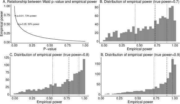
Figure 13: A. Relationship between Wald test empirical power and p-value. B-D. Distribution of empirical power given 70% (B), 80% (C), 90% (D) study power. The dashed line indicates median power and dotted lines the 25th and 75th quantiles.

To understand this intuitively, consider the relationship between significance testing and power estimation. A significance test assesses whether a coefficient of interest exceeds some threshold. Power is a measure of the probability that the coefficient of interest exceeds that threshold when the study is replicated an infinite number of times. If a low p-value is observed, that provides some evidence that the coefficient may be large. However, with only a single study, we have no way to discern whether the coefficient is actually large, and power is high; or whether the coefficient was large by random chance in our study, but in truth is smaller. Power is an average of whether a coefficient is statistically significant over infinite study replications ($n=\infty$). By contrast, empirical “power” is a single draw from that distribution ($n=1$), a point estimate for which we cannot calculate variance.

We illustrate this with the example of a one-sample Wald test in Figure 13, Panels B-D. Each histogram shows the distribution of empirical power from a Wald test, with the underlying study power varying from 70% to 90%. While the median study drawn from an underlying distribution has the correct empirical power, there is a considerable variance in empirical power across study replications. From a single study, we have no way to discern whether the empirical power of 90% came from a study with 90% power or one with 70% power. Furthermore, given publication bias toward studies with higher statistical significance, which inflates effect size, we will likely observe low p-values (i.e. high empirical power) far more than would be expected in published studies, suggesting empirical power will often be artificially inflated. Other tests may have different distributions of empirical power, but there is a similar bijective relationship between empirical power and p-value.

References

- (1)
- Abadie (2018) Abadie, Alberto, “Statistical Non-Significance in Empirical Economics,” Working Paper 24403, National Bureau of Economic Research March 2018.
- Alpert et al. (2019) Alpert, Abby E, William N Evans, Ethan M.J. Lieber, and David Powell, “Origins of the Opioid Crisis and Its Enduring Impacts,” Working Paper 26500, National Bureau of Economic Research November 2019.
- Altman and Bland (1995) Altman, Douglas G. and J. Martin Bland, “Statistics notes: Absence of evidence is not evidence of absence,” BMJ, August 1995, 311 (7003), 485.
- Angrist and Pischke (2009) Angrist, Joshua David and Jörn-Steffen Pischke, Mostly Harmless Econometrics: An Empiricist’s Companion, Princeton: Princeton University Press, 2009. OCLC: ocn231586808.
- Akosa Antwi et al. (2013) Antwi, Yaa Akosa, Asako S. Moriya, and Kosali Simon, “Effects of Federal Policy to Insure Young Adults: Evidence from the 2010 Affordable Care Act’s Dependent-Coverage Mandate,” American Economic Journal: Economic Policy, November 2013, 5 (4), 1–28.
- Barbaresco et al. (2015) Barbaresco, Silvia, Charles J. Courtemanche, and Yanling Qi, “Impacts of the Affordable Care Act dependent coverage provision on health-related outcomes of young adults,” Journal of Health Economics, March 2015, 40, 54–68.
- Black et al. (2019) Black, Bernard, Alex Hollingsworth, Leticia Nunes, and Kosali Simon, “The Effect of Health Insurance on Mortality: Power Analysis and What We Can Learn from the Affordable Care Act Coverage Expansions,” Working Paper 25568, National Bureau of Economic Research February 2019.
- Cantor et al. (2012) Cantor, Joel C., Alan C. Monheit, Derek DeLia, and Kristen Lloyd, “Early Impact of the Affordable Care Act on Health Insurance Coverage of Young Adults,” Health Services Research, 2012, 47 (5), 1773–1790.
- Clogg et al. (1995) Clogg, Clifford C., Eva Petkova, and Adamantios Haritou, “Statistical Methods for Comparing Regression Coefficients Between Models,” American Journal of Sociology, March 1995, 100 (5), 1261–1293.
- Daw and Hatfield (2018) Daw, Jamie R. and Laura A. Hatfield, “Matching and Regression to the Mean in Difference-in-Differences Analysis,” Health Services Research, 2018, 53 (6), 4138–4156. Dependent Health Coverage and Age for Healthcare Benefits
- Dependent Health Coverage and Age for Healthcare Benefits (n.d.) Dependent Health Coverage and Age for Healthcare Benefits.
- Duflo (2001) Duflo, Esther, “Schooling and Labor Market Consequences of School Construction in Indonesia: Evidence from an Unusual Policy Experiment,” American Economic Review, September 2001, 91 (4), 795–813.
- Freyaldenhoven et al. (2019) Freyaldenhoven, Simon, Christian Hansen, and Jesse M. Shapiro, “Pre-event Trends in the Panel Event-Study Design,” American Economic Review, September 2019, 109 (9), 3307–3338.
- Gelman (2019) Gelman, Andrew, “Don’t Calculate Post-hoc Power Using Observed Estimate of Effect Size,” Annals of Surgery, January 2019, 269 (1), e9.
- Ghosh et al. (2017) Ghosh, Ausmita, Kosali Simon, and Benjamin D Sommers, “The Effect of State Medicaid Expansions on Prescription Drug Use: Evidence from the Affordable Care Act,” Working Paper 23044, National Bureau of Economic Research January 2017.
- Goldman et al. (2018) Goldman, Anna L., Danny McCormick, Jennifer S. Haas, and Benjamin D. Sommers, “Effects Of The ACA’s Health Insurance Marketplaces On The Previously Uninsured: A Quasi-Experimental Analysis,” Health Affairs, April 2018, 37 (4), 591–599.
- Hahn (2012) Hahn, Seokyung, “Understanding noninferiority trials,” Korean Journal of Pediatrics, November 2012, 55 (11), 403–407.
- Hartman and Hidalgo (2018) Hartman, Erin and F. Daniel Hidalgo, “An Equivalence Approach to Balance and Placebo Tests,” American Journal of Political Science, 2018.
- Hatfield and Zeldow (n.d.) Hatfield, Laura and Bret Zeldow, “Difference-in-Differences.”
- Hausman (1978) Hausman, J. A., “Specification tests in econometrics,” Econometrica, 1978, 46 (6), 1251–1271.
- Hoenig and Heisey (2001) Hoenig, John M and Dennis M Heisey, “The Abuse of Power: The Pervasive Fallacy of Power Calculations for Data Analysis,” The American Statistician, February 2001, 55 (1), 19–24.
- Hoynes et al. (2016) Hoynes, Hilary, Diane Whitmore Schanzenbach, and Douglas Almond, “Long-Run Impacts of Childhood Access to the Safety Net,” American Economic Review, April 2016, 106 (4), 903–934.
- Ioannidis et al. (2017) Ioannidis, John P.A., T. D. Stanley, and Hristos Doucouliagos, “The Power of Bias in Economics Research,” The Economic Journal, October 2017, 127 (605), F236–F265.
- Kahn-Lang and Lang (2018) Kahn-Lang, Ariella and Kevin Lang, “The Promise and Pitfalls of Differences-in-Differences: Reflections on ‘16 and Pregnant’ and Other Applications,” Working Paper 24857, National Bureau of Economic Research July 2018.
- Kohn (2015) Kohn, Sally, “Five reasons Americans already love ObamaCare — plus one reason why they’re gonna love it even more, soon,” March 2015.
- Levine and Ensom (2001) Levine, Marc and Mary H. H. Ensom, “Post Hoc Power Analysis: An Idea Whose Time Has Passed?,” Pharmacotherapy: The Journal of Human Pharmacology and Drug Therapy, 2001, 21 (4), 405–409.
- McCrary (2008) McCrary, Justin, “Manipulation of the running variable in the regression discontinuity design: A density test,” Journal of Econometrics, February 2008, 142 (2), 698–714.
- Mora and Reggio (2012) Mora, Ricardo and Iliana Reggio, “Treatment effect identification using alternative parallel assumptions,” 2012.
- Muralidharan and Prakash (2017) Muralidharan, Karthik and Nishith Prakash, “Cycling to School: Increasing Secondary School Enrollment for Girls in India,” American Economic Journal: Applied Economics, July 2017, 9 (3), 321–350.
- Rokicki et al. (2018) Rokicki, Slawa, Jessica Cohen, Günther Fink, Joshua A. Salomon, and Mary Beth Landrum, “Inference With Difference-in-Differences With a Small Number of Groups: A Review, Simulation Study, and Empirical Application Using SHARE Data,” Medical Care, January 2018, 56 (1), 97.
- Roth (2019) Roth, Jonathan, “Pre-test with Caution: Event-study Estimates After Testing for Parallel Trends?,” 2019.
- Roth and Rambachan (2019) and Ashesh Rambachan, “An Honest Approach to Parallel Trends,” 2019.
- Ryan et al. (2019) Ryan, Andrew M, Evangelos Kontopantelis, Ariel Linden, and James F Burgess, “Now trending: Coping with non-parallel trends in difference-in-differences analysis,” Statistical Methods in Medical Research, December 2019, 28 (12), 3697–3711.
- Sommers et al. (2013) Sommers, Benjamin D., Thomas Buchmueller, Sandra L. Decker, Colleen Carey, and Richard Kronick, “The Affordable Care Act Has Led To Significant Gains In Health Insurance And Access To Care For Young Adults,” Health Affairs, January 2013, 32 (1), 165–174.
- Suest (n.d.) Suest, Technical Report.
- Tavernise (2012) Tavernise, Sabrina, “More Young Adults Have Health Insurance, Study Says,” The New York Times, September 2012.
- Wasserstein and Lazar (2016) Wasserstein, Ronald L. and Nicole A. Lazar, “The ASA’s Statement on p -Values: Context, Process, and Purpose,” The American Statistician, April 2016, 70 (2), 129–133.
- Weesie (2000) Weesie, Jeroen, “Seemingly unrelated estimation and the cluster-adjusted sandwich estimator,” Stata Technical Bulletin, February 2000, 9.
- Wolfers (2006) Wolfers, Justin, “Did Unilateral Divorce Laws Raise Divorce Rates? A Reconciliation and New Results,” American Economic Review, December 2006, 96 (5), 1802–1820.
- Yurukoglu et al. (2017) Yurukoglu, Ali, Eli Liebman, and David B. Ridley, “The Role of Government Reimbursement in Drug Shortages,” American Economic Journal: Economic Policy, May 2017, 9 (2), 348–382.