Efficient Shortest Paths in Scale-Free Networks with Underlying Hyperbolic Geometry

Abstract

A standard approach to accelerating shortest path algorithms on networks is the bidirectional search, which explores the graph from the start and the destination, simultaneously. In practice this strategy performs particularly well on scale-free real-world networks. Such networks typically have a heterogeneous degree distribution (e.g., a power-law distribution) and high clustering (i.e., vertices with a common neighbor are likely to be connected themselves). These two properties can be obtained by assuming an underlying hyperbolic geometry.

To explain the observed behavior of the bidirectional search, we analyze its running time on hyperbolic random graphs and prove that it is $\mathcal{\tilde{O}}(n^{2-1/\alpha}+n^{1/(2\alpha)}+\delta_{\max})$ with high probability, where $\alpha\in(1/2,1)$ controls the power-law exponent of the degree distribution, and $\delta_{\max}$ is the maximum degree. This bound is sublinear, improving the obvious worst-case linear bound. Although our analysis depends on the underlying geometry, the algorithm itself is oblivious to it.

1 Introduction

One of the most fundamental graph problems consists of finding a shortest path between two vertices in a network. Besides being of independent interest, many algorithms use shortest path queries as a subroutine. On unweighted graphs, such queries can be answered in linear time using a breadth-first search (BFS). Though this is optimal in the worst case, it is not efficient enough when dealing with large networks or problems involving many shortest path queries.

A way to heuristically improve the run time, is to use a bidirectional BFS [26]. It runs two searches, simultaneously exploring the graph from the start and the destination. The shortest path is found once the two search spaces touch. Being one of the standard heuristics, the bidirectional BFS is widely used in practice (e.g., in route planning). On homogeneous networks (where most vertices have similar degrees, like road networks) this typically leads to a speedup factor of about two. However, on heterogeneous networks (having many vertices of low degree and only few vertices of very high degree, like social networks or the internet) experiments indicate that the bidirectional BFS yields an asymptotic running time improvement [10].

Despite being such a fundamental heuristic, theory completely fails its main purpose of predicting and explaining the observed behavior. The theoretical worst case running time overshoots the observations by a lot. A more promising approach is the average-case analysis by Borassi and Natale [10], which considers instances that are drawn from certain probability distributions instead of assuming the worst case. Their results are summarized in the first row of Table 1. The analysis covers a variety of random graph models. On the one hand these include homogeneous networks where the degree distribution has bounded variance, e.g. Erdős-Rényi random graphs. On the other hand, they also consider heterogeneous networks where the variance of the degree distribution is unbounded, e.g. Chung-Lu random graphs with power-law exponent $\beta\in(2,3)$. However, the results, again, do not match what is observed in practice, as it predicts shorter running times on homogeneous networks than on heterogeneous ones.

	Homogeneous	Heterogeneous
Independent Edges	Bounded Variance $m^{\frac{1}{2}+o(1)}$ [10]	Unbounded Variance $m^{\frac{4-\beta}{2}+o(1)}$ [10]
Underlying Geometry	Euclidean Random Graphs $\Theta(n)$ (Folklore)	Hyperbolic Random Graphs $\tilde{\mathcal{O}}(n^{2\frac{\beta-2}{\beta-1}}+n^{\frac{1}{\beta-1}})$ (This paper)

Table 1: Probabilistic bounds on the running time of the bidirectional BFS obtained by analyzing different random graph models. The considered models (and associated results) are arranged by the heterogeneity of the corresponding degree distributions of the graphs and the (in)dependence of edges. Here, $n$ and $m$ denote the number of vertices and edges in the graph, respectively. The parameter $\beta\in(2,3)$ denotes the power-law exponent of the degree distribution in the considered heterogeneous networks.

The fundamental obstacle that prevents the average-case analysis from producing convincing explanations is that the considered random graph models are not realistic. They assume that edges in the graph are independent of each other. However, real-world networks typically exhibit locality, i.e., edges in an evolving network tend to form between vertices that are already close in the network.

We resolve this discrepancy by modeling edge dependencies using geometry and extend the comparison in Table 1 by adding the second row. Generally, geometric random graphs are obtained by randomly distributing vertices in some metric space (e.g. the Euclidean plane) and connecting any two vertices with a probability that depends on their distance. In this framework, heterogeneous networks (i.e., networks on which the bidirectional BFS has been observed to perform particularly well) can be obtained by using the hyperbolic plane as the underlying geometry.

In this paper, we analyze the bidirectional BFS on random graph models with an underlying geometry. We prove that, with high probability, the bidirectional BFS has a sublinear worst-case running time on the heterogeneous networks generated by the hyperbolic random graph model. Additionally, it is not hard to see why there is no asymptotic speedup on the homogeneous networks generated by the Euclidean random graph model. Both results match previous empirical observations. Finally, we interpret these insights and discuss how the heterogeneity of the degree distribution and an underlying geometry affect the running time of the bidirectional breadth first search.

Related Work

The research on scale-free networks has gained a lot of attention for quite some time now. Therefore, it is no surprise that the extensively studied problem of computing shortest paths has also been considered in the context of such graphs [1, 23, 20]. However, the bidirectional search that was introduced in 1969 [26] and that has since become one of the standard search heuristics, has only recently been examined on scale-free networks. In fact, there are only two theoretical explanations for the performance improvements obtained using this heuristic, both using an average-case analysis that considers one or more random graph models [21, 10].

A model that yields a better representation of real-world networks than the ones considered before, is the hyperbolic random graph model introduced by Krioukov et al. [19]. The generated graphs feature a heterogeneous degree distribution, high clustering, and a small diameter; properties that are often observed in real-world networks. These properties emerge naturally from the hyperbolic geometry. Moreover, the model is conceptually simple, which makes it accessible to mathematical analysis. For these reasons it has gained popularity in different research areas and has been studied from different perspectives.

From the network-science perspective, the goal is to gather knowledge about real-world networks. This is, for example, achieved by assuming that a real-world network has a hidden underlying hyperbolic geometry, which can be revealed by embedding it into the hyperbolic plane [2, 9].

From the mathematical perspective, the focus lies on studying structural properties. The degree distribution and clustering [17], diameter [15, 22], component structure [8, 18], clique size [6], and separation properties [5] have been studied successfully.

Additionally, there is the algorithmic perspective, which is the focus of this paper. Usually algorithms are analyzed by proving worst-case running times. Though this is the strongest possible performance guarantee, it is rather pessimistic as practical instances rarely resemble worst-case instances. Techniques leading to a more realistic analysis include parameterized or average-case complexity. The latter is based on the assumption that instances are drawn from a certain probability distribution. For hyperbolic random graphs, the maximum clique, as well as the minimum vertex cover can be computed in polynomial time [6, 3], and there are several algorithmic results based on the fact that hyperbolic random graphs have sublinear tree width [5]. Moreover, there is a compression algorithm that can store a hyperbolic random graph using $\mathcal{O}(n)$ bits in expectation [12, 25]. Finally, a close approximation of the shortest path between two vertices can be found using greedy routing, which visits only $\mathcal{O}(\log\log n)$ vertices for most start–destination pairs [13]. The downside of most of these algorithms is that they need to know the underlying geometry, i.e., the coordinates of each vertex, which is a rather unrealistic assumption for real-world networks. In contrast to that, we analyze an algorithm that is oblivious to the underlying geometry.

Outline

After a brief introduction to hyperbolic random graphs in Section 2, we examine the bidirectional BFS in Section 3. We start by briefly arguing why the bidirectional BFS gives no asymptotic speedup over the standard BFS on Euclidean random graphs in Section 3.2. Afterwards, in Section 3.3 we rigorously analyze the bidirectional BFS on hyperbolic random graphs. Section 4 contains concentration bounds that were left out in Section 3 to improve readability. In Section 5, we conclude by comparing our theoretical results to empirical data and interpret them.

2 Preliminaries

Let $G=(V,E)$ be an undirected and unweighted graph. We denote the number of vertices and edges with $n$ and $m$, respectively. The neighborhood of a vertex $v\in V$ is $N(v)=\{w\in V\leavevmode\nobreak\ |\leavevmode\nobreak\ \{v,w\}\in E\}$. The degree of $v$ is $\deg(v)=|N(v)|$. We denote the maximum degree with $\delta_{\max}$. The soft $\mathcal{O}$-notation $\mathcal{\tilde{O}}$ suppresses poly-logarithmic factors in $n$.

2.1 The Hyperbolic Plane

The major difference between hyperbolic and Euclidean geometry is the exponential expansion of space. In the hyperbolic plane, a circle of radius $r$ has area $2\pi(\cosh(r)-1)$ and circumference $2\pi\sinh(r)$, with $\cosh(x)=(e^{x}+e^{-x})/2$ and $\sinh(x)=(e^{x}-e^{-x})/2$, both growing as $e^{x}/2\pm o(1)$. To identify points, we use polar coordinates with respect to a designated origin $O$ and a ray starting at $O$. A point $p$ is uniquely determined by its radius $r$, which is the distance to $O$, and the angle (or angular coordinate) $\varphi$ between the reference ray and the line through $p$ and $O$. In illustrations, we use the native representation, obtained by interpreting the hyperbolic coordinates as polar coordinates in the Euclidean plane; see Figure 1 (left). Due to the exponential expansion, line segments bend towards the origin $O$.

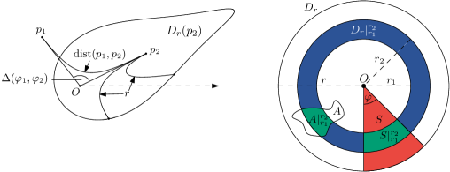
Figure 1: Left: Points and several line segments in the native representation of the hyperbolic plane. A disk of radius $r$ is centered at $p_{2}$. Right: Geometric shapes and their intersections. Sector $S$ has an angular width of $\varphi$.

Let $p_{1}=(r_{1},\varphi_{1})$ and $p_{2}=(r_{2},\varphi_{2})$ be two points. The angular distance between $p_{1}$ and $p_{2}$ is the angle between the rays from the origin through $p_{1}$ and $p_{2}$. Formally, it is $\Delta(\varphi_{1},\varphi_{2})=\pi-|\pi-|\varphi_{1}-\varphi_{2}||$. The hyperbolic distance $\operatorname{dist}(p_{1},p_{2})$ is given by

$$\cosh(\operatorname{dist}(p_{1},p_{2}))=\cosh(r_{1})\cosh(r_{2})-\sinh(r_{1})\sinh(r_{2})\cos(\Delta(\varphi_{1},\varphi_{2})).$$

Note how the angular coordinates make simple definitions cumbersome as angles are considered modulo $2\pi$, leading to a case distinction depending on where the reference ray lies. Whenever possible, we implicitly assume that the reference ray was chosen such that we do not have to compute modulo $2\pi$. Thus, the above angular distance between $p_{1}$ and $p_{2}$ simplifies to $|\varphi_{1}-\varphi_{2}|$. A third point $p=(r,\varphi)$ lies between $p_{1}$ and $p_{2}$ if $\Delta(\varphi,\varphi_{1})+\Delta(\varphi,\varphi_{2})=\Delta(\varphi_{1},\varphi_{2})$.

Throughout the paper, we regularly use different geometric shapes that are mostly based on disks centered at the origin $O$, as can be seen in Figure 1 (right). With $D_{r}(p)$ we denote the disk of radius $r$ around a point $p$, i.e., the set of points that have distance $r$ to $p$. For disks, that are centered in the origin $O$, we simplify the notation and set $D_{r}\coloneqq D_{r}(O)$. The restriction of a disk $D_{r}$ to all points with angular coordinates in a certain interval is called sector, which we usually denote with the letter $S$. Its angular width is the length of this interval. For an arbitrary set of points $A$, we use $A|_{r_{1}}^{r_{2}}$ to denote the restriction of $A$ to points with radii in $[r_{1},r_{2}]$, i.e., $A|_{r_{1}}^{r_{2}}=A\cap(D_{r_{2}}\setminus D_{r_{1}})$.

2.2 Hyperbolic Random Graphs

A hyperbolic random graph is generated by drawing $n$ points uniformly at random in a disk of the hyperbolic plane and connecting pairs of points whose distance is below a threshold. More precisely, the model depends on two parameters $C$ and $\alpha$ that are assumed to be constants. The generated graphs have a power-law degree distribution with power-law exponent $\beta=2\alpha+1$ and a constant average degree depending on $C$. The parameter $\alpha$ is assumed to be in the range $(1/2,1)$, yielding power-law exponents $\beta\in(2,3)$. Exponents outside of this range are atypical for hyperbolic random graphs. For $\beta<2$ the average degree of the generated networks diverges, while for $\beta>3$ the graphs decompose into small components (of size sublinear in $n$) and the variance of the degree distribution is no longer unbounded. In contrast, it is unbounded for $\beta\in(2,3)$, resulting in very heterogeneous degree distributions. Moreover, in this range the obtained networks have a giant component of size $\Omega(n)$ [7], and all other components have at most polylogarithmic size with high probability [15, Corollary 13]. Note that a bidirectional BFS could completely explore a non-giant component in $\tilde{\mathcal{O}}(1)$ time and either return the shortest path (if both vertices are in the same non-giant component) or conclude that the vertices are in different components. Therefore, we only consider the case when the two considered vertices are both in the giant component in the remainder of the paper.

When generating a hyperbolic random graph, the $n$ points are sampled within the disk $D_{R}$ of radius $R=2\log n+C$. For each vertex, the angular coordinate is drawn uniformly from $[0,2\pi]$. Its radius $r$ is sampled according to the probability density function $f(r)$, which can then be used to define the joint distribution of angles and radii $f(r,\varphi)$. They are given by

$$f(r)=\frac{\alpha\sinh(\alpha r)}{\cosh(\alpha R)-1}=\Theta(e^{-\alpha(R-r)})\leavevmode\nobreak\ \quad\text{and}\leavevmode\nobreak\ \quad f(r,\varphi)=\frac{1}{2\pi}f(r)$$ (1)

for $r\in[0,R]$. For $r>R$, $f(r)=f(r,\varphi)=0$. Two vertices are connected by an edge if and only if their hyperbolic distance is at most $R$. The above probability distribution is a natural choice as the probability for a vertex ending up in a certain region is proportional to its area (at least for $\alpha=1$). Note that the exponential growth in $r$ reflects the fact that the area of a disk grows exponentially with the radius. It follows that a hyperbolic random graph has few vertices with high degree close to the center of the disk and many vertices with low degree near its boundary. The following lemma is common knowledge; for the sake of completeness we give a short proof.

Lemma 2.1.

Let $G$ be a hyperbolic random graph. Furthermore, let $v_{1},v_{2}$ be two vertices with radii $r_{1}\leq r_{2}\leq R$, respectively, and with the same angular coordinate. Then $N(v_{2})\subseteq N(v_{1})$.

Proof 2.2.

Let $w\in N(v_{2})$, i.e., $\operatorname{dist}(v_{2},w)\leq R$. Now consider the triangle $v_{2}Ow$, which is completely contained in the disk of radius $R$ around $w$ (since $\operatorname{dist}(v_{2},w)\leq R$ and $r(w)\leq R$). Since disks are convex and $v_{1}$ lies on the line from $O$ to $v_{2}$, it is part of the triangle and therefore also contained in this disk. Consequently, $\operatorname{dist}(v_{1},w)\leq R$ and thus $w\in N(v_{1})$.

Given two vertices with fixed radii $r_{1}$ and $r_{2}$, their hyperbolic distance grows with increasing angular distance. The maximum angular distance such that they are still adjacent [17, Lemma 3.1] is

$$\theta(r_{1},r_{2}) =\arccos\left(\frac{\cosh(r_{1})\cosh(r_{2})-\cosh(R)}{\sinh(r_{1})\sinh(r_{2})}\right)$$

$$=2e^{\frac{R-r_{1}-r_{2}}{2}}(1+\Theta(e^{R-r_{1}-r_{2}})),$$ (2)

assuming $r_{2}\geq R-r_{1}$. Otherwise, we have $r_{1}+r_{2}<R$, meaning two vertices with these radii are adjacent, independent of their angular distance.

The probability that a sampled vertex falls into a given subset $A\subseteq D_{R}$ of the disk is given by its probability measure $\mu(A)=\iint_{A}f(r,\varphi)\operatorname{d\!}\varphi\operatorname{d\!}r$, which can be thought of as the area of $A$. There are two types of regions we encounter regularly: disks $D_{r}$ with radius $r$ centered at the origin and disks $D_{R}(r,\varphi)$ of radius $R$ centered at a point $(r,\varphi)$. Note that the measure of $D_{R}(r,\varphi)$ gives the probability that a random vertex lies in the neighborhood of a vertex with position $(r,\varphi)$. Gugelmann et al. [17, Lemma 3.2] showed that

$$\mu(D_{r})=e^{-\alpha(R-r)}(1+o(1)),\text{ and}$$ (3)

$$\mu(D_{R}(r,\varphi))=\Theta(e^{-r/2}).$$ (4)

For a given region $A\subseteq D_{R}$ of the disk, let $X_{1},\dots,X_{n}$ be random variables with $X_{i}=1$ if vertex $i$ lies in $A$ and $X_{i}=0$ otherwise. Then $X=\sum_{i=1}^{n}X_{i}$ is the number of vertices lying in $A$. By the linearity of expectation, we obtain that the expected number of vertices in $A$ is $\mathbb{E}[X]=\sum_{i=1}^{n}\mathbb{E}[X_{i}]=n\mu(A)$.

Often, determining the expected value of a random variable is not sufficient to obtain meaningful statements. Therefore, we additionally classify events depending on how likely they are to occur. We say that an event holds with high probability, if it occurs with probability $1-\mathcal{O}(1/n)$. Moreover, we say that an event holds asymptotically almost surely if it occurs with probability $1-o(1)$.

To show that certain random variables are concentrated around their expectation (i.e., with high probability the outcome does not deviate much from the expected value) we regularly use the following Chernoff-Hoeffding bound.

Theorem 2.3 (Chernoff Bound [14, Theorem 1.1]).

Let $X_{1},\dots,X_{n}$ be independent random variables with $X_{i}\in\{0,1\}$ and let $X$ be their sum. Then,

$$\Pr[X>t] \leq 2^{-t} t>2e\mathbb{E}[X]$$ for  and

$$\Pr[X<(1-\varepsilon)\mathbb{E}[X]] \leq e^{-\varepsilon^{2}/2\cdot\mathbb{E}[X]} \text{for $\varepsilon\in(0,1)$}.$$

Usually, it suffices to show that a random variable does not exceed a certain upper bound or drop below a lower bound with high probability. The following corollaries show that sufficiently large upper and lower bounds on the expected value suffice to obtain concentration.

Corollary 2.4.

Let $X_{1},\dots,X_{n}$ be independent random variables with $X_{i}\in\{0,1\}$ and let $X$ be their sum. Further, let $f(n)=\Omega(\log(n))$ be such that $\mathbb{E}[X]\leq f(n)$ and let $c$ be a constant. Then, $X=\mathcal{O}(f(n))$ holds with probability $1-O(n^{-c})$.

Proof 2.5.

We prove the statement by showing that the probability for the complementary event (i.e., $X$ is more than a constant factor larger than $f(n)$) is $\mathcal{O}(n^{-c})$ for any $c$. Since $\mathbb{E}[X]\leq f(n)$, we can choose a constant $c_{1}$ sufficiently large such that $c_{1}f(n)>2e\mathbb{E}[X]$. Thus, by Theorem 2.3 it holds that

$$\Pr[X>c_{1}f(n)]\leq 2^{-c_{1}f(n)}.$$

Moreover, we have $f(n)=\Omega(\log n)$. Consequently, there exists another constant $c_{2}$ such that $f(n)\geq c_{2}\log n$ for sufficiently large $n$. We obtain

$$\Pr[X>c_{1}f(n)]\leq 2^{-c_{1}c_{2}\log n}\leq n^{-c_{1}c_{2}}$$

for $n$ sufficiently large. Finally, we can chose $c_{1}$ such that $c_{1}>c/c_{2}$, which yields the claim.

Corollary 2.6.

Let $X_{1},\dots,X_{n}$ be independent random variables with $X_{i}\in\{0,1\}$ and let $X$ be their sum. Further, let $f(n)=\omega(\log n)$ be such that $f(n)\leq\mathbb{E}[X]$ and let $c$ be a constant. Then, $X\in\Omega(f(n))$ holds with probability $1-O(n^{-c})$.

Proof 2.7.

Analogous to the proof of Corollary 2.4 we prove the statement by showing that the probability for the complementary event (i.e., $X$ is more than a constant factor smaller than $f(n)$) is $\mathcal{O}(n^{-c})$ for any $c$. Let $\varepsilon$ be a constant with $\varepsilon\in(0,1)$. The following inequalities are obtained by first using the fact that $f(n)\leq\mathbb{E}[X]$, applying the second statement of Theorem 2.3, again applying $f(n)\leq\mathbb{E}[X]$, and finally using $f(n)\in\omega(\log n)$:

$$\Pr[X<(1-\varepsilon)f(n)] \leq\Pr[X<(1-\varepsilon)\mathbb{E}[X]]$$

$$\leq e^{-\varepsilon^{2}/2\cdot\mathbb{E}[X]}$$

$$\leq e^{-\varepsilon^{2}/2\cdot f(n)}$$

$$=e^{-\varepsilon^{2}/2\cdot\omega(\log n)}$$

$$=n^{-\omega(1)}.$$

Finally, the following lemma shows that statements about the neighborhood of a vertex with fixed angular coordinate can be extended to hold for arbitrary angular coordinates, with a small penalty in certainty.

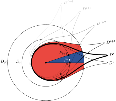
Figure 2: Visualization of the proof of Lemma 2.8. When constrained to the disk $D_{R}$, the disk $D^{\prime}$ (bold) with center $P^{\prime}$ at radius $r$ is completely contained in two consecutive disks $D^{i}$ and $D^{i+1}$ (red region). Point $P_{i}$ is between $P$ and $P^{\prime}$.

Lemma 2.8.

Let $G$ be a hyperbolic random graph, let $X_{w}\geq 0$ for $w\in V$ be random variables, and let $X(D)=\sum_{w\in D}X_{w}$ for $D\subseteq D_{R}$. Further, let $\boldsymbol{D}_{R}(r)$ be the set of disks of radius $R$ with center at radius $r$. If for each $D\in\boldsymbol{D}_{R}(r)$ it holds that $\Pr[X(D)\leq f(n)]\geq 1-p$, then $\Pr[\forall D\in\boldsymbol{D}_{R}(r)\colon X(D)\leq 2f(n)]\geq 1-\mathcal{O}(np)$.

Proof 2.9.

Let $D^{\prime}\in\boldsymbol{D}_{R}(r)$ be a disk with radius $R$ centered at radius $r$ and arbitrary angular coordinate. To bound $X(D^{\prime})$, we cover the disk $D_{R}$ with a circular sequence of $n^{\prime}$ disks $D^{1},\dots,D^{n^{\prime}}$, such that $D^{\prime}$ is completely contained in two consecutive disks (when constrained to the whole disk $D_{R}$). That is, there exists an $i\in\{1,\dots,n^{\prime}\}$ such that $D^{\prime}\subseteq D^{i}\cup D^{i+1}$. Since $X_{w}\geq 0$ for all $w\in V$, it then holds that

$$X(D^{\prime})=\sum_{w\in D^{\prime}}X_{w}\leq\sum_{D^{i}\cup D^{i+1}}X_{w}\leq\sum_{w\in D^{i}}X_{w}+\sum_{w\in D^{i+1}}X_{w}=X(D^{i})+X(D^{i+1}).$$

Since $\Pr[X(D)\leq f(n)]\geq 1-p$ holds for each $D\in\boldsymbol{D}_{R}(r)$, we can apply the union bound to conclude that $X(D^{i})\leq f(n)$ holds for all $i\in\{0,\dots,n^{\prime}\}$ with probability $1-n^{\prime}p$. Consequently, $X(D^{\prime})\leq 2f(n)$ with probability $1-n^{\prime}p$.

To complete the proof, it remains to show that there exists such a sequence $D^{1},\dots,D^{n^{\prime}}$ with $n^{\prime}\in\mathcal{O}(n)$. See Figure 2 for an illustration of how the sequence is constructed. All disks $D^{i}$ for $i\in\{1,\dots,n^{\prime}\}$ have their center at radius $r$. The center of the first disk is placed at angular coordinate $0$ and each subsequent disk is placed at an angular distance of $2\theta(r,R)$ (see Equation (2.2)) to its predecessor until the whole disk is covered. Note that, as a consequence, the boundaries of two consecutive disks intersect at the boundary of the whole disk $D_{R}$.

Let $P^{\prime}$ be the center of $D^{\prime}$. To see that $D^{\prime}$ is contained in two consecutive disks $D^{i}$ and $D^{i+1}$ (when constrained to the whole disk $D_{R}$), first note that there exists an $i\in\{1,\dots,n^{\prime}\}$ such that $P^{\prime}$ is between the centers $P_{i}$ and $P_{i+1}$ of two consecutive disks $D^{i}$ and $D^{i+1}$. We show that any point $P\in D^{\prime}$ is contained in $D^{i}\cup D^{i+1}$. Clearly, $D^{i}\cup D^{i+1}$ contains all points between $P_{i}$ and $P_{i+1}$ (blue region in Figure 2). For the case where $P$ does not lie between $P_{i}$ and $P_{i+1}$, assume without loss of generality, that $P_{i}$ is between $P$ and $P^{\prime}$, as depicted in Figure 2. Since $\operatorname{dist}(P,P^{\prime})\leq R$ and since $P^{\prime}$ and $P_{i}$ have the same radius but $P_{i}$ is between $P$ and $P^{\prime}$, it follows that $\operatorname{dist}(P,P_{i})\leq R$, and thus $P\in D^{i}$. Finally, it remains to show that $n^{\prime}=\mathcal{O}(n)$ disks are sufficient to cover the whole disk $D_{R}$. Since two consecutive disks are placed at an angular distance of $2\theta(r,R)$, we need $n^{\prime}=2\pi/(2\theta(r,R))=\mathcal{O}(1/\theta(r,R))$ disks. Since $\theta(r,R)\geq\theta(R,R)$, it follows that $n^{\prime}=\mathcal{O}(1/\theta(R,R))=\mathcal{O}(e^{R/2})$ due to Equation (2.2). Substituting $R=2\log(n)+C$ then yields the claim.

3 Bidirectional Breadth-First Search

Figure 3: Visualization of the two phases of each BFS in a hyperbolic random graph. Vertices that are visited during the first phase are red. The red edges denote the first encounter of a vertex in the inner disk $D_{R}|_{0}^{\rho}$ (green region). This corresponds to the first step in the second phase. The last step then leads to a common neighbor via the blue edges.

In this section, we analyze the running time of the bidirectional BFS and obtain an upper bound on the maximum running time over all possible start–destination pairs. Our results are summarized in the following main theorem.

Theorem 3.1.

Let $G$ be a hyperbolic random graph. With high probability the shortest path between any two vertices in $G$ can be computed in $\mathcal{\tilde{O}}(n^{2-1/\alpha}+n^{1/(2\alpha)}+\delta_{\max})$ time.

We note that this bound on the running time also holds in expectation. Our bound fails with probability $\mathcal{O}(1/n)$, in which case the worst-case running time is still bounded by the size of the hyperbolic random graph, which is $\mathcal{O}(n)$. Consequently, this case contributes $\mathcal{O}(1)$ to the expectation, which is dominated by the above bound.

To prove Theorem 3.1, we make use of the hyperbolic geometry in the following way; see Figure 3. As long as the two searches visit only low-degree vertices, all explored vertices lie within a small region, i.e., the searches operate locally. Once the searches visit high-degree vertices closer to the center of the hyperbolic disk (green area in Figure 3), it takes only few steps to complete the search, as hyperbolic random graphs have a densely connected core. Thus, we split our analysis in two phases: a first phase in which both searches advance towards the center and a second phase in which both searches meet in the center. Note that this strategy assumes that we know the coordinates of the vertices as we would like to stop a search once it reached the center. To resolve this issue, we first show in Section 3.1 that there exists an alternation strategy that is oblivious to the geometry but performs not much worse than any other alternation strategy. We note that this result is independent of hyperbolic random graphs and thus interesting in its own right. Afterwards, in Section 3.2 we examine the performance of the bidirectional BFS on Euclidean random graphs, before focusing on hyperbolic random graphs in Section 3.3.

3.1 Bidirectional Search and Alternation Strategies

In an unweighted and undirected graph $G=(V,E)$, a BFS finds the shortest path between two vertices $s,t\in V$ by starting at $s$ and exploring the graph in levels, where the $i$th level $L^{s}_{i}$ contains the vertices with distance $i$ to $s$. More formally, the BFS starts with the set $L^{s}_{0}=\{s\}$ on level $0$. Assuming the levels $L^{s}_{0},\dots,L^{s}_{i}$ have been computed already, one obtains the next level $L^{s}_{i+1}$ as the set of neighbors of vertices in level $L^{s}_{i}$ that are not contained in earlier levels. Computing $L^{s}_{i+1}$ from $L^{s}_{i}$ is called an exploration step, obtained by exploring the edges between vertices in $L^{s}_{i}$ and $L^{s}_{i+1}$.

The bidirectional BFS runs two BFSs simultaneously. The forward search starts at $s$ and the backward search starts at $t$. The shortest path between the two vertices can then be obtained, once the search spaces of the forward and backward search touch. Since the two searches cannot actually be run simultaneously, they alternate depending on their progress. When exactly the two searches alternate is determined by the alternation strategy. Note that we only swap after full exploration steps, i.e., we never explore only half of level $i$ of one search before continuing with the other. This has the advantage that we can be certain to know the shortest path once a vertex is found by both searches.

In the following we define the greedy alternation strategy as introduced by Borassi and Natale [10] and show that it is not much worse than any other alternation strategy. Assume the latest levels of the forward and backward searches are $L^{s}_{i}$ and $L^{t}_{j}$, respectively. Then the next exploration step of the forward search would cost time proportional to $c^{s}_{i}\coloneqq\sum_{v\in L^{s}_{i}}\deg(v)$, while the cost for the backward search is $c^{t}_{j}\coloneqq\sum_{v\in L^{t}_{j}}\deg(v)$. The greedy alternation strategy then greedily continues with the search that causes the fewer cost in the next exploration step, i.e., it continues with the forward search if $c^{s}_{i}\leq c^{t}_{j}$ and with the backward search otherwise.

Theorem 3.2.

Let $G$ be a graph with diameter $d$. If there exists an alternation strategy such that the bidirectional BFS explores $f(n)$ edges, then the bidirectional BFS with greedy alternation strategy explores at most $d\cdot f(n)$ edges.

Proof 3.3.

Let $A$ be the alternation strategy that explores only $f(n)$ edges. First note that the number of explored edges only depends on the number of levels explored by the two different searches and not on the actual order in which they are explored. Thus, if the greedy alternation strategy is different from $A$, we can assume without loss of generality that the greedy strategy performed more exploration steps in the forward search and fewer in the backward search compared to $A$. Let $c^{s}$ and $c^{t}$ be the number of edges explored by the forward and backward search, respectively, when using the greedy strategy. Moreover, let $j$ be the last level of the backward search (which is actually not explored) and, accordingly, let $c^{t}_{j}$ be the number of edges the next step in the backward search would have explored. Then $c^{t}+c^{t}_{j}\leq f(n)$ as, when using $A$, the backward search still explores level $j$. Moreover, the forward search with the greedy strategy explores at most $c^{t}+c^{t}_{j}$ (and therefore at most $f(n)$) edges in each step, as exploring the backward search would be cheaper otherwise. Consequently, each step in the forward and backward search costs at most $f(n)$. As there are at most $d$ steps in total, we obtain the claimed bound.

3.2 Bidirectional Search in Euclidean Random Graphs

Euclidean random graphs, commonly known as random geometric graphs, are generated by distributing $n$ vertices uniformly at random in the unit square $[0,1]^{2}$ and connecting any two vertices if the Euclidean distance between them is at most some threshold $R\in\mathbb{R}$ [24]. One can imagine, that each vertex is equipped with a disk of radius $R$ and an edge is added to all other vertices that lie in this disk. The threshold $R$ affects the properties of the generated network and in order to obtain graphs with a giant component of linear size (as is the case for hyperbolic random graphs), $R$ has to be chosen from the so called supercritical regime [24]. In contrast to hyperbolic random graphs, the uniform sampling of the vertices in the Euclidean space leads to a distribution where the number of vertices falling into each disk is roughly the same, which in turn leads to a homogeneous degree distribution.

We examine how a BFS explores such a graph, by considering the region of the plane containing the vertices visited after several exploration steps. For Euclidean random graphs with $R$ chosen from the supercritical regime it was shown that for two vertices at graph theoretic distance $d$, it holds that $R\cdot d$ is at most a constant factor larger than the Euclidean distance between them, if $d$ is super-logarithmic [16]. Additionally, it is easy to see that the Euclidean distance between them can be at most $R\cdot d$. Therefore, we can assume that after $k$ (sufficiently many) steps the region in the plane that contains the visited vertices resembles a disk of radius proportional to $k$. Since the area of a disk with radius $r$ grows as $\pi r^{2}$, the expected number of explored vertices is in $\Theta(nk^{2})$ (since the vertices are distributed uniformly).

In this scenario it is easy to see that the performance of a bidirectional BFS improves by a constant factor, compared to a standard BFS. Let $s$ and $t$ be two vertices with (sufficiently large) graph theoretic distance $d$ from each other. Then, the expected number of vertices explored by a standard BFS from $s$ to $t$ is $\Theta(nd^{2})$. If we run two searches instead (one starting at $s$, the other at $t$), then the expected explored search space is minimized when the two BFSs touch after half as many steps, exploring two disks of half the radius. (Note that this holds independent of the chosen alternation strategy.) In that case the expected number of explored vertices is proportional to $2n\pi(d/2)^{2}$ which is again $\Theta(nd^{2}$), indicating that the bidirectional variant yields no asymptotic speedup over the standard BFS.

In the remainder of this paper we focus on the performance of the bidirectional BFS on hyperbolic random graphs. In contrast to Euclidean random graphs, they feature a heterogeneous degree distribution, leading to significant differences in the performance of the bidirectional BFS.

3.3 Bidirectional Search in Hyperbolic Random Graphs

To analyze the size of the search space of the bidirectional BFS in hyperbolic random graphs, we separate the whole disk $D_{R}$ into two parts. One is the inner disk $D_{R}|_{0}^{\rho}$ centered at the origin. Its radius $\rho$ is chosen in such a way that any two vertices in $D_{R}|_{0}^{\rho}$ have a common neighbor with high probability. The second part is the outer band $D_{R}|_{\rho}^{R}$, the remainder of the whole disk. A single BFS now explores the graph in two phases. In the first phase, the BFS explores vertices in the outer band. The phase ends, when the next vertex to be encountered lies in the inner disk. Once both BFSs completed the first phase, they only need at most two more steps for their search spaces to share a vertex. One step to encounter the vertex in the inner disk and another step to meet at their common neighbor that any two vertices in the inner disk have with high probability; see Figure 3.

Note that this scenario describes the worst case. Depending on the positions of the two considered vertices the two searches may touch earlier, e.g., when both vertices are close to each other in the outer band or when at least one of them is already contained in the inner disk. However, since we want to determine an upper bound on the running time, we consider the case where both vertices lie in the outer band and the two searches touch in the inner disk. In the remainder of the paper we only consider how one of the two searches explores the graph. The obtained bounds also hold for the other search, meaning the total search space increases only by a constant factor when considering both searches instead of only one.

For our analysis we assume an alternation strategy in which each search stops once it explored one additional level after finding the first vertex in the inner disk $D_{R}|_{0}^{\rho}$. Of course, this cannot be implemented without knowing the underlying geometry of the network. However, by Theorem 3.2 the search space explored using the greedy alternation strategy is only a poly-logarithmic factor larger, as the diameter of hyperbolic random graphs is poly-logarithmic with high probability [15]. The following lemma shows for which choice of $\rho$ the above sketched strategy works.

Lemma 3.4.

Let $G$ be a hyperbolic random graph. With high probability, $G$ contains a vertex that is adjacent to every other vertex in $D_{R}|_{0}^{\rho}$, for $\rho=\frac{1}{\alpha}(\log n-\log\log n)$.

Proof 3.5.

Assume $v$ is a vertex with radius at most $R-\rho$. Note that the distance between two points is upper bounded by the sum of their radii. Thus, every vertex in $D_{R}|_{0}^{\rho}$ has distance at most $R$ to $v$, and is therefore adjacent to $v$. Hence, to prove the claim, it suffices to show the existence of this vertex $v$ with radius at most $R-\rho$. As described in Section 2, the probability for a single vertex to have radius at most $R-\rho$ is given by the measure $\mu(D_{R}|_{0}^{R-\rho})$. Using Equation (3) we obtain

$$\mu(D_{R}|_{0}^{R-\rho}) =e^{-\alpha\rho}(1+o(1))=\frac{\log n}{n}(1+o(1)).$$

Thus, the probability that none of the $n$ vertices lies in $D_{R}|_{0}^{R-\rho}$ is given by $(1-\mu(D_{R}|_{0}^{R-\rho}))^{n}$. That is,

$$\Pr[\{v\in D_{R}|_{0}^{R-\rho}\}=\emptyset]=\left(1-\frac{\log n}{n}(1+o(1))\right)^{n}.$$

Since $(1-x)\leq e^{-x}$ for all $x\in\mathbb{R}$, this term can be bounded by

$$\Pr[\{v\in D_{R}|_{0}^{R-\rho}\}=\emptyset] \leq e^{-\frac{\log(n)}{n}(1+o(1))\cdot n}=e^{-\log(n)(1+o(1))}=n^{-(1+o(1))}=\mathcal{O}(1/n).$$

Hence, there is at least one vertex with radius at most $R-\rho$ with high probability.

In the following, we first bound the search space explored in the first phase, i.e., before we enter the inner disk $D_{R}|_{0}^{\rho}$. Afterwards we bound the search space explored in the second phase, which consists of two exploration steps. The first one to enter $D_{R}|_{0}^{\rho}$ and the second one to find a common neighbor, which exists due to Lemma 3.4.

3.3.1 Search Space in the First Phase

To bound the size of the search space in the outer band, we make use of the geometry in the following way. For two vertices in the outer band to be adjacent, their angular distance has to be small. Moreover, the number of exploration steps is bounded by the diameter of the graph. Thus, the maximum angular distance between vertices visited in the first phase cannot be too large. Note that the following lemma restricts the search to a sublinear portion of the disk, which we later use to show that also the number of explored edges is sublinear.

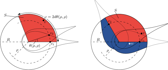
Figure 4: Left: The sector $S$ (red) of angular width $\varphi$ contains the search space of a BFS starting at $v$, in the outer band $D_{R}|_{\rho}^{R}$. The vertices $v_{1}$ and $v_{2}$ are at maximum angular distance to still be adjacent. Right: Neighbor $w$ of vertex $v$ is in $S$ (red) or a neighbor of $c_{1}$ or $c_{2}$ (blue).

Lemma 3.6.

With high probability, all vertices that a BFS on a hyperbolic random graph explores before finding a vertex with radius at most $\rho=\frac{1}{\alpha}(\log n-\log\log n)$ lie within a sector of angular width $\mathcal{\tilde{O}}(n^{-(1/\alpha-1)})$.

Proof 3.7.

For an illustration of the proof see Figure 4 (left). Recall from Section 2 that $\theta(r_{1},r_{2})$ denotes the maximum angular distance between two vertices of radii $r_{1}$ and $r_{2}$ such that they are still adjacent. Since $r_{1}$ and $r_{2}$ only appear as negative exponents in the expression for $\theta(r_{1},r_{2})$ (see Equation (2.2)), this angle increases with decreasing radii. Thus, $\theta(r_{1},r_{2})\leq\theta(\rho,\rho)$ holds for all vertices in the outer band $D_{R}|_{\rho}^{R}$.

Now assume we start a BFS at a vertex $v\in D_{R}|_{\rho}^{R}$ and perform $d$ exploration steps without leaving the outer band $D_{R}|_{\rho}^{R}$. Then no explored vertex has angular distance more than $d\theta(\rho,\rho)$ from $v$. Thus, the whole search space lies within a disk sector of angular width $2d\theta(\rho,\rho)$. The number of steps $d$ is at most poly-logarithmic as the diameter of a hyperbolic random graph is poly-logarithmic with high probability [15]. Using Equation (2.2) for $\theta(\rho,\rho)$, we obtain

$$\theta(\rho,\rho) =2e^{\frac{R-2\rho}{2}}(1+\Theta(e^{R-2\rho}))$$

$$=2e^{C/2}n^{1-1/\alpha}\log(n)^{1/\alpha}(1+\Theta((\log n/n^{1-\alpha})^{2/\alpha}))$$

$$=\mathcal{O}(n^{-(1/\alpha-1)}\log(n)^{1/\alpha}),$$

which proves the claimed bound.

Note that the expected number of vertices in a sector $S$ of angular width $\varphi$ is linear in $n\varphi$ due to the fact that the angular coordinate of each vertex is chosen uniformly at random. Thus, Lemma 3.6 already shows that the expected number of vertices visited in the first phase of the BFS is $\mathcal{\tilde{O}}(n^{2-1/\alpha})$, which is sublinear in $n$. It is also not hard to see that this bound holds with high probability (see Corollary 2.4). To also bound the number of explored edges, we sum the degrees of vertices in $S$. It is not surprising that this yields the same asymptotic bound in expectation, as the expected average degree in a hyperbolic random graph is constant. However, to obtain meaningful results, we need a bound that holds with high probability. Though we can use techniques similar to those that have been used to show that the average degree of the whole graph is constant with high probability [11, 17], the situation is complicated by the restriction to a sublinear portion of the disk. Nonetheless, we obtain the following theorem.

Theorem 3.8.

Let $G$ be a hyperbolic random graph. The degrees of vertices in every sector of angular width $\varphi$ sum to $\mathcal{\tilde{O}}(\varphi n+n^{1/(2\alpha)}+\delta_{\max})$ with high probability if $\varphi=\Omega(\log(n)^{2}/n^{1/2}).$

We note that $\delta_{\max}$ has to be included here, as the theorem states a bound for every sector, and thus in particular for sectors containing the vertex of maximum degree. Recall, that $\delta_{\max}=\mathcal{\tilde{O}}(n^{1/(2\alpha)})$ holds almost surely [17]. Moreover, we note that the condition $\varphi=\Omega(\log(n)^{2}/n^{1/2})$ is crucial for our proof, i.e., the angular width of the sector has to be sufficiently large for the concentration bound to hold. We note that, depending on $\alpha$, the angular width determined in Lemma 3.6 may be smaller than this lower bound. However, if this is the case, we can choose $\varphi=\mathcal{\tilde{O}}(n^{-1/2})$ as an upper bound for the angular width of the sector and obtain $\mathcal{\tilde{O}}(\varphi n)=\mathcal{\tilde{O}}(n^{1/2})=\mathcal{\tilde{O}}(n^{1/(2\alpha)})$ for $\alpha\in(1/2,1)$. Consequently, the bound holds for the previously determined angular width $\mathcal{\tilde{O}}(n^{-(1/\alpha-1)})$ for all $\alpha\in(1/2,1)$.

As the proof for Theorem 3.8 is rather technical, we defer it to Section 4. Together with Lemma 3.6, we obtain the following corollary. Note that since $\alpha\in(1/2,1)$, this shows that the running time spend in the first phase (not accounting for the maximum degree) is sublinear in $n$ with high probability.

Corollary 3.9.

On a hyperbolic random graph, the first phase of the bidirectional search explores with high probability only $\mathcal{\tilde{O}}(n^{2-1/\alpha}+n^{1/(2\alpha)}+\delta_{\max})$ many edges.

3.3.2 Search Space in the Second Phase

The first phase of the BFS is completed when the next vertex to be encountered lies in the inner disk. Thus, the second phase consists of only two exploration steps. One step to encounter the vertex in the inner disk and another step to meet the other search. Thus, to bound the running time of the second phase, we have to bound the number of edges explored in these two exploration steps. To do this, let $V_{1}$ be the set of vertices encountered in the first phase. Recall that all these vertices lie within a sector $S$ of angular width $\varphi=\mathcal{\tilde{O}}(n^{-(1/\alpha-1)})$ (Lemma 3.6). The number of explored edges in the second phase is then bounded by the sum of degrees of all neighbors $N(V_{1})$ of vertices in $V_{1}$. To bound this sum, we divide the neighbors of $V_{1}$ into two categories: $N(V_{1})\cap S$ and $N(V_{1})\setminus S$. Note that we already bounded the sum of degrees of vertices in $S$ for the first phase (see Theorem 3.8), which clearly also bounds this sum for $N(V_{1})\cap S$. Thus, it remains to bound the sum of degrees of vertices in $N(V_{1})\setminus S$.

To bound this sum, we introduce two hypothetical vertices (i.e., vertices with specific positions that are not actually part of the graph) $c_{1}$ and $c_{2}$ such that every vertex in $N(V_{1})\setminus S$ is a neighbor of $c_{1}$ or $c_{2}$. Then it remains to bound the sum of degrees of neighbors of these two vertices. To define $c_{1}$ and $c_{2}$, recall that the first phase was restricted to points in the sector $S$ that have a radius greater than $\rho$, i.e., all vertices in $V_{1}$ lie within $S|_{\rho}^{R}$. The hypothetical vertices $c_{1}$ and $c_{2}$ are basically positioned at the corners of this region, i.e., they both have radius $\rho$, and they assume the maximum and minimum angular coordinate within $S$, respectively. Figure 4 (right) shows these positions. We obtain the following.

Lemma 3.10.

Let $G$ be a hyperbolic random graph, let $S$ be a sector, and let $v\in S|_{\rho}^{R}$ be a vertex. Then, every neighbor of $v$ lies in $S$ or is a neighbor of one of the hypothetical vertices $c_{1}$ or $c_{2}$.

Proof 3.11.

Let $v=(r,\varphi)\in S|_{\rho}^{R}$ and $w\in N(v)\setminus S$. Without loss of generality, assume that $c_{1}$ lies between $v$ and $w$, as is depicted in Figure 4 (right). Now consider the point $v^{\prime}=(\rho,\varphi)$ obtained by moving $v$ to the same radius as $c_{1}$. According to Lemma 2.1 we have $N(v)\subseteq N(v^{\prime})$. In particular, it holds that $w\in N(v^{\prime})$ and therefore $\operatorname{dist}(v^{\prime},w)\leq R$. Since $v^{\prime}$ and $c_{1}$ have the same radial coordinate and $c_{1}$ is between $v^{\prime}$ and $w$, it follows that $\operatorname{dist}(c_{1},w)\leq R$.

By the above argument, it remains to sum the degrees of neighbors of $c_{1}$ and $c_{2}$. In the following, we show that the degrees of the neighbors of a vertex with radius $r$ sum to $\Theta(ne^{-(\alpha-1/2)r})$ in expectation. We note that, for large values of $r$, i.e., for a vertex lying close to the boundary of the disk, this term is surprisingly large. This is due to the fact that, although vertices near the center of the disk are rather unlikely to exist in the first place, their degree would be sufficiently large such that they dominate the expected degree sum.

Lemma 3.12.

Let $G$ be a hyperbolic random graph. The degrees of the neighbors of a vertex $v$ sum to $\Theta(ne^{-(\alpha-1/2)r(v)})$ in expectation.

Proof 3.13.

Let $Z_{v}$ be the sum of the degrees of the neighbors of $v$, which is a random variable that depends on the positions of all vertices in the graph. Formally, we can express $Z_{v}$ by assigning each vertex $w\in V\setminus\{v\}$ two random variables $X_{w}$ and $Y_{w}$. The first is an indicator random variable with $X_{w}=1$ if $w$ is a neighbor of $v$ and $X_{w}=0$ otherwise. Additionally, the random variable $Y_{w}$ denotes the degree of $w$. The sum of the degrees of the neighbors of $v$ can then be written as

$$Z_{v}=\sum_{w\in V\setminus\{v\}}X_{w}\cdot Y_{w}.$$

The expected value of $Z_{v}$ is given by

$$\mathbb{E}[Z_{v}]=\mathbb{E}\left[\sum_{w\in V\setminus\{v\}}X_{w}\cdot Y_{w}\right]=\sum_{w\in V\setminus\{v\}}\mathbb{E}\left[X_{w}\cdot Y_{w}\right],$$

where the second equality holds due to the linearity of expectation. To compute the expected value of $X_{w}\cdot Y_{w}$ we can apply the law of total expectation and obtain

$$\mathbb{E}[Z_{v}]=\sum_{w\in V\setminus\{v\}}\sum_{x\in\{0,1\}}\mathbb{E}[X_{w}\cdot Y_{w}\mid X_{w}=x]\cdot\Pr[X_{w}=x].$$

Clearly, the case where $X_{w}=0$ does not contribute anything to the sum, which can thus be simplified as

$$\mathbb{E}[Z_{v}]=\sum_{w\in V\setminus\{v\}}\mathbb{E}[Y_{w}\mid X_{w}=1]\cdot\Pr[X_{w}=1].$$

Recall that $X_{w}=1$ denotes the event where $w$ is a neighbor of $v$. That is,

$$\Pr[X_{w}=1]=\Pr[w\in N(v)]=\Pr[w\in D_{R}(v)]=\mu(D_{R}(v)).$$

Moreover, recall that $Y_{w}$ denotes the random variable representing the degree of $w$. Consequently, we can now write $\mathbb{E}[Z_{v}]$ as

$$\mathbb{E}[Z_{v}] =\sum_{w\in V\setminus\{v\}}\mu(D_{R}(v))\cdot\mathbb{E}[Y_{w}\mid w\in D_{R}(v)]$$

$$=(n-1)\cdot\mu(D_{R}(v))\cdot\mathbb{E}[\deg(w)\mid w\in D_{R}(v)].$$ (5)

We continue by computing the expected degree of a vertex $w$ conditioned on the fact that it is contained in $D_{R}(v)$. To this end, we first consider the expected value without the condition, analogous to how it was done previously [17] (see the proof of Theorem 2.3), and afterwards explain how to incorporate the condition. The expected degree of a vertex $w$ with fixed radius $r$ is given by

$$\mathbb{E}[\deg(w)\mid r(w)=r]=(n-1)\mu(D_{R}(w)).$$

To obtain the expected degree of $w$ without fixing its radius (or angle for that matter) we then integrate $\mathbb{E}[\deg(w)\mid r(w)=r\wedge\varphi(w)=\varphi]\cdot f(r,\varphi)$ (note the joint distribution) over the whole disk. That is,

$$\mathbb{E}[\deg(w)] =\iint_{D_{R}}\mathbb{E}[\deg(w)\mid r(w)=r\wedge\varphi(w)=\varphi]\cdot f(r,\varphi)\operatorname{d\!}\varphi\operatorname{d\!}r$$

$$=\iint_{D_{R}}\mathbb{E}[\deg(w)\mid r(w)=r]\cdot f(r,\varphi)\operatorname{d\!}\varphi\operatorname{d\!}r,$$

where the second step follows from the fact that the expected degree of a vertex is independent of its angular coordinate.

It remains to include the condition on the fact that $w$ cannot be anywhere in the whole disk but lies in $D_{R}(v)$ instead. First, we have to accommodate for the fact that if $w$ is a neighbor of $v$, then conversely $v$ is also a neighbor of $w$. Consequently, we know that $w$ has at least one neighbor, which we reflect in the expected value by introducing the condition on the position $p(v)$ of $v$. Moreover, in general the conditional expectation of a random variable $X$ conditioned on an event $A$ (with $\Pr[A]>0$) is given by $\mathbb{E}[X\mid A]=\int_{-\infty}^{\infty}xf_{X\mid A}(x)\operatorname{d\!}x$, where $f_{X\mid A}$ is defined as

$$f_{X\mid A}(x)=\begin{cases}\frac{f_{X}(x)}{\Pr[A]},&x\in A,\\ 0,&x\notin A.\end{cases}$$

Therefore, the above expression for the expected degree of $w$ can be adjusted to include the condition as

$$\mathbb{E}[\deg(w)\mid w\in D_{R}(v)] =\iint_{D_{R}(v)}\mathbb{E}[\deg(w)\mid r(w)=r\wedge p(v)=(r,\varphi)]$$

$$\hphantom{=\iint_{D_{R}(v)}\leavevmode\nobreak\ }\cdot\frac{f(r,\varphi)}{\Pr[w\in D_{R}(v)]}\operatorname{d\!}\varphi\operatorname{d\!}r.$$

Note that the probability $\Pr[w\in D_{R}(v)]$ in the denominator is, again, the measure of the disk of radius $R$ centered at $v$. Substituting this expression in Equation (3.13) for the expected sum $\mathbb{E}[Z_{v}]$ of the degrees of the neighbors of $v$, we get

$$\mathbb{E}[Z_{v}] =(n-1)\cdot\mu(D_{R}(v))\cdot\mathbb{E}[\deg(w)\mid w\in D_{R}(v)]$$

$$=(n-1)\cdot\mu(D_{R}(v))\cdot$$

$$\hphantom{=(n-1\cdot\leavevmode\nobreak\ )}\cdot\iint_{D_{R}(v)}\mathbb{E}[\deg(w)\mid r(w)=r\wedge p(v)=(r,\varphi)]\frac{f(r,\varphi)}{\mu(D_{R}(v))}\operatorname{d\!}\varphi\operatorname{d\!}r$$

$$=(n-1)\cdot\iint_{D_{R}(v)}\mathbb{E}[\deg(w)\mid r(w)=r\wedge p(v)=(r,\varphi)]\cdot f(r,\varphi)\operatorname{d\!}\varphi\operatorname{d\!}r.$$

To compute the integral, we determine the expected degree of $w$ conditioned on the fact that $r(w)=r$ and on the position of $v$, which is a neighbor of $w$ deterministically. Therefore, we obtain the expected degree by adding $1$ (for $v$) to the expected number of vertices among the remaining $V\setminus\{v,w\}$ that are sampled into $D_{R}(w)$ and obtain

$$\mathbb{E}[\deg(v)\mid r(w)=r\wedge p(v)=(r,\varphi)]=1+(n-2)\mu(D_{R}(w)),$$

which is $1+\Theta(ne^{-r/2})$ due to Equation (4). Note that $\Theta(ne^{-r/2})$ is $\Omega(1)$ for all $r\in[0,R]$, allowing us to further simplify the expected value to

$$\mathbb{E}[\deg(v)\mid r(w)=r\wedge p(v)=(r,\varphi)]=\Theta(ne^{-r/2}).$$

Moreover, recall that $f(r,\varphi)=0$ for $r>R$ and that it can otherwise be bounded by $f(r,\varphi)=\Theta(e^{-\alpha(R-r)})$ (see Equation (1)). We obtain

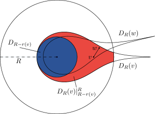
Figure 5: Situation in the proof of Lemma 3.12. Vertex $w$ is a neighbor of $v$. To integrate $D_{R}(v)\cap D_{R}$, we split the region into two parts: $D_{R}(v)|_{0}^{R-r(v)}=D_{R-r(v)}$ (blue) and $D_{R}(v)|_{R-r(v)}^{R}$ (red).

$$\mathbb{E}[Z_{v}] =\Theta\left((n-1)\cdot\iint_{D_{R}(v)\cap D_{R}}ne^{-r/2}\cdot e^{-\alpha(R-r)}\operatorname{d\!}\varphi\operatorname{d\!}r\right)$$

$$=\Theta\left(n^{2}e^{-\alpha R}\cdot\iint_{D_{R}(v)\cap D_{R}}e^{(\alpha-1/2)r}\operatorname{d\!}\varphi\operatorname{d\!}r\right).$$

We can now split the integral into two parts: one containing the disk $D_{R}(v)|_{0}^{R-r(v)}=D_{R-r(v)}$ and the other containing the remainder of $D_{R}(v)\cap D_{R}$, which is given by $D_{R}(v)|_{R-r(v)}^{R}$ (see Figure 5). For the second part we can use Equation (2.2) to bound the angle $\theta(r(v),r)$ up to which we need to integrate depending on $r$. As a result, we get

$$\mathbb{E}[Z_{v}] =\Theta\Bigg{(}n^{2}e^{-\alpha R}\cdot\Bigg{(}\int_{0}^{R-r(v)}\int_{0}^{2\pi}e^{(\alpha-1/2)r}\operatorname{d\!}\varphi\operatorname{d\!}r$$

$$\hphantom{=\Theta\Bigg{(}n^{2}e^{-\alpha R}\cdot\Bigg{(}\leavevmode\nobreak\ }+\int_{R-r(v)}^{R}\int_{0}^{\theta(r(v),r)}e^{(\alpha-1/2)r}\operatorname{d\!}\varphi\operatorname{d\!}r\Bigg{)}\Bigg{)}.$$

Regarding the first part of the sum, note that evaluating the inner integral only contributes a constant factor that can be dropped due the $\Theta$-notation. Computing the outer integral then yields $\Theta(e^{(\alpha-1/2)(R-r(v))})$. For the second part of the sum we, again, first evaluate the inner integral and substitute $\theta(r(v),r)=\Theta(e^{(R-r(v)-r)/2})$ (see Equation (2.2)). We obtain

$$\mathbb{E}[Z_{v}] =\Theta\left(n^{2}e^{-\alpha R}\cdot\left(e^{(\alpha-1/2)(R-r(v))}+e^{(R-r(v))/2}\int_{R-r(v)}^{R}e^{-(1-\alpha)r}\operatorname{d\!}r\right)\right).$$

The last integral evaluates to $\mathcal{O}(e^{-(1-\alpha)(R-r(v))})$, which multiplied by the factor $e^{(R-r(v))/2}$ yields asymptotically the same expression as the first summand and we get

$$\mathbb{E}[Z_{v}] =\Theta\left(n^{2}e^{-(\alpha-1/2)r(v)}\cdot e^{-R/2}\right).$$

Finally, we can substitute $R=2\log(n)+C$ in order to obtain the claimed bound of $\mathbb{E}[Z_{v}]=\Theta(ne^{-(\alpha-1/2)r(v)})$.

For $c_{1}$ and $c_{2}$, which both have radius $\rho$, the degrees of their neighbors thus sum to $\mathcal{\tilde{O}}(n^{1/(2\alpha)})$ in expectation. However, to actually prove Theorem 3.1, we need a bound that holds with high probability for all possible angular coordinates of $c_{1}$ and $c_{2}$. As with the sum of the degrees in a sector, we prove a slightly weaker bound that matches the one in Theorem 3.1 and holds with high probability. We obtain the following lemma.

Lemma 3.14.

Let $G$ be a hyperbolic random graph and let $v$ be a hypothetical vertex with radius $\rho=1/\alpha(\log n-\log\log n)$ and arbitrary angular coordinate. The degrees of neighbors of $v$ sum to $\mathcal{\tilde{O}}(n^{2-1/\alpha}+n^{1/(2\alpha)}+\delta_{\max})$ with high probability.

Again, the proof is rather technical and thus deferred to Section 4. Together with the bounds on the sum of degrees in a sector of width $\varphi=\mathcal{\tilde{O}}(n^{-(1/\alpha-1)})$ (Theorem 3.8), we obtain the following corollary, which concludes the proof of Theorem 3.1.

Corollary 3.15.

On a hyperbolic random graph, the second phase of the bidirectional search explores with high probability only $\mathcal{\tilde{O}}(n^{2-1/\alpha}+n^{1/(2\alpha)}+\delta_{\max})$ many edges.

4 Concentration Bounds for the Sum of Vertex Degrees

Here we prove the concentration bounds that were announced in the previous section. For the first phase, we already know that the search space is contained within a sector $S$ of sublinear width (Lemma 3.6). Thus, the running time in the first phase is bounded by the sum of vertex degrees in this sector. Moreover, all edges explored in the second phase also lie within the same sector $S$ or are incident to neighbors of the two hypothetical vertices $c_{1}$ and $c_{2}$ (Lemma 3.10). Thus, the running time of the second phase is bounded by the sum of vertex degrees in $S$ and in the neighborhood of $c_{1}$ and $c_{2}$.

In both cases, we have to bound the sum of vertex degrees in certain areas of the disk, which can be done as follows. For each degree, we want to compute the number of vertices of this degree in the considered area and multiply it with the degree. As all vertices with a certain degree have roughly the same radius, we can separate the disk into small bands, one for each degree. Then summing over all degrees comes down to summing over all bands and multiplying the number of vertices in this band with the corresponding degree. If we can prove that each of these values is highly concentrated (i.e., holds with probability $1-\mathcal{O}(n^{-2})$), we obtain that the sum is concentrated as well (using the union bound). Unfortunately, this fails in two situations. For small radii, the number of vertices within the corresponding band (i.e., the number of high degree vertices) is too small to be concentrated. Moreover, for large radii the degree is too small to be concentrated around its expected value.

To overcome this issue, we partition the disk $D_{R}$ into three parts. An inner part $D_{R}|_{0}^{\rho_{I}(\varphi)}$, containing all points of radius at most $\rho_{I}(\varphi)$, an outer part $D_{R}|_{\rho_{O}}^{R}$, containing all points of radius at least $\rho_{O}$, and a central part $D_{R}|_{\rho_{I}(\varphi)}^{\rho_{O}}$, containing all points in between. We choose $\rho_{I}(\varphi)$ such that the number of vertices with maximum degree in a sector part $S|_{\rho_{I}(\varphi)}^{\rho_{O}}$ of angular width $\varphi$ is $\Omega(\log n)$, which ensures that for each vertex degree, the number of vertices with this degree is concentrated. Moreover, we choose $\rho_{O}$ in such a way that the vertex degrees in $S|_{\rho_{I}(\varphi)}^{\rho_{O}}$ are sufficiently concentrated. To achieve this, we set

$$\rho_{I}(\varphi)=R-\frac{1}{\alpha}\left(\log(\varphi/(2\pi))+\log n-\log\log n\right)\text{ and }\,\rho_{O}=R-(2+\varepsilon)\log\log(n),$$

for any constant $\varepsilon\in(0,1)$, and show concentration for the sum of the degrees in a sector and in the neighborhood of a vertex with radius $\rho$, separately for the three parts of the disk.

4.1 The Inner Part of the Disk

The inner part $D_{R}|_{0}^{\rho_{I}(\varphi)}$ contains vertices of high degree. It is not hard to see that there are only logarithmically many vertices with radius at most $\rho_{I}(\varphi)$.

Lemma 4.1.

Let $G$ be a hyperbolic random graph, let $\varphi\in[0,2\pi]$ be an angle, and let $\xi>0$ be a constant. A sector $S|_{0}^{\rho_{I}(\varphi)}$ of angular width $\xi\varphi\in[0,2\pi]$ contains $\mathcal{O}(\log(n))$ vertices, with probability $1-\mathcal{O}(n^{-c})$ for any constant $c$.

Proof 4.2.

By Equation (3) the expected number of vertices in the disk $D_{R}|_{0}^{\rho_{I}(\varphi)}$ is given by

$$\mathbb{E}[|\{v\in D_{R}|_{0}^{\rho_{I}(\varphi)}\}|]=ne^{-\alpha(R-\rho_{I}(\varphi))}(1+o(1)).$$

Since the angular coordinates of the vertices are distributed uniformly in $[0,2\pi]$, the expected number of vertices in a sector portion $S|_{0}^{\rho_{I}(\varphi)}$ of angular width $\xi\varphi$ is

$$\mathbb{E}[|\{v\in S|_{0}^{\rho_{I}(\varphi)}\}|] =\frac{\xi\varphi}{2\pi}ne^{-\alpha(R-\rho_{I}(\varphi))}(1+o(1))$$

$$=\frac{\xi\varphi}{2\pi}ne^{-(\log(\varphi/2\pi)+\log n-\log\log n)}(1+o(1))$$

$$=\xi\log(n)(1+o(1)).$$

Since $\xi>0$ is constant, this bound is in $\Omega(\log n)$ and we can apply Corollary 2.4 to conclude that $|\{v\in S|_{0}^{\rho_{I}(\varphi)}\}|=\mathcal{O}(\log(n))$ holds with probability $1-\mathcal{O}(n^{-c})$ for any constant $c$.

Note that, if $\varphi\in\Omega(1/n)$, we can choose at most $\mathcal{O}(n)$ sectors of width $2\varphi$ such that any sector of width $\varphi$ lies completely in one of them. Thus, the probability that there exists a sector portion $S|_{0}^{\rho_{I}(\varphi)}$ where the number of vertices is super-logarithmic, is bounded by the probability that it is too large in at least one of these $\mathcal{O}(n)$ sectors (of twice the width). By choosing $\xi=2$, we can apply Lemma 4.1 to conclude that a single sector $S|_{0}^{\rho_{I}(\varphi)}$ of twice the angular width contains at most $\mathcal{O}(\log(n))$ vertices with probability $1-\mathcal{O}(n^{-2})$. Applying the union bound and incorporating the fact that the maximum degree in the graph is $\delta_{\max}$ we can bound the number of edges in every such sector portion and obtain the following corollary.

Corollary 4.3.

Let $G$ be a hyperbolic random graph. For every sector $S$ of angular width $\varphi\in\Omega(1/n)$, the degrees of the vertices in $S|_{0}^{\rho_{I}(\varphi)}$ sum to $\mathcal{\tilde{O}}(\delta_{\max})$ with high probability.

Note that, in particular the statement holds for the previously determined angle $\varphi=\mathcal{\tilde{O}}(n^{-(1/\alpha-1)})$ for $\alpha\in(1/2,1)$. Additionally, by setting $\varphi=2\pi$, we can use Lemma 4.1 to bound the sum of the degrees of the high degree vertices in the neighborhood of a vertex with radius $\rho$.

Corollary 4.4.

Let $G$ be a hyperbolic random graph. For every vertex $v$ of radius $\rho$, the degrees of the neighbors of $v$ in $D_{R}|_{0}^{\rho_{I}(2\pi)}$ sum to $\mathcal{\tilde{O}}(\delta_{\max})$ with high probability.

4.2 The Central Part of the Disk

For each possible vertex degree $k$, we want to compute the number of vertices with this degree in the central part $D_{R}|_{\rho_{I}(\varphi)}^{\rho_{O}}$. First note, that by Equation (4) a vertex with fixed radius has expected degree $\Theta(k)$ if this radius is $2\log(n/k)$. Motivated by this, we define $r_{k}=2\log(n/k)$. To bound the sum of degrees in the central part $D_{R}|_{\rho_{I}(\varphi)}^{\rho_{O}}$, we use that vertices with radius significantly larger than $r_{k}$ also have a smaller degree. To this end, we first prove that a vertex with degree $k$ can actually not have a radius much larger than $r_{k}$. This has the advantage, that we can bound the number of degree-$k$ vertices by bounding the number of vertices with these radii.

Lemma 4.5.

Let $G$ be a hyperbolic random graph. Then, for every constant $c>0$, there exist constants $\kappa,\tau>0$, such that all vertices with degree at least $k\geq\kappa\log n$ have radius at most $r_{k}+\tau$ with probability $1-\mathcal{O}(n^{-c})$.

Proof 4.6.

To prove this lemma, it suffices to show that there exist constants $\kappa,\tau>0$, such that the probability of a vertex with radius greater than $r_{k}+\tau$ having degree at least $k$, i.e. $\Pr[\exists v\in V\colon\deg(v)\geq k\land r(v)\geq r_{k}+\tau]$, is small. To obtain the following sequence of inequalities, we first use the union bound, then apply the definition of conditional probabilities, and finally use Lemma 2.1.

$$\Pr[\exists v\in V\colon\deg(v)\geq k\land r(v)\geq r_{k}+\tau] \leq n\cdot\Pr[\deg(v)\geq k\land r(v)\geq r_{k}+\tau]$$

$$\leq n\cdot\Pr[\deg(v)\geq k\leavevmode\nobreak\ |\leavevmode\nobreak\ r(v)\geq r_{k}+\tau]$$

$$\leq n\cdot\Pr[\deg(v)\geq k\leavevmode\nobreak\ |\leavevmode\nobreak\ r(v)=r_{k}+\tau].$$

To prove the statement of the lemma, it remains to show that $\Pr[\deg(v)\geq k\mid r(v)=r_{k}+\tau]$ is sufficiently small, i.e., in $\mathcal{O}(n^{-(c+1)})$.

Recall that, by Equation (4), the expected degree of a vertex with radius $r$ is in $\Theta(ne^{-r/2})$. For a vertex $v$ with radius $r_{k}+\tau$ we obtain $ne^{-(r_{k}+\tau)/2}=e^{-\tau/2}k$. It follows that there exists a constant $c^{\prime}>0$, such that $\mathbb{E}[\deg(v)]\leq c^{\prime}e^{-\tau/2}k$. By choosing $\tau$ large enough we can ensure that $k\geq 2e\mathbb{E}[\deg(v)]$, allowing us to apply the Chernoff-Hoeffding bound in Theorem 2.3. We obtain $\Pr[\deg(v)\geq k]\leq 2^{-k}$. Finally, since $k\geq\kappa\log n$, we can choose $\kappa$ such that this probability is bounded by $\mathcal{O}(n^{-(c+1)})$.

We are now ready to bound the number of vertices in a sector that have degree at least $k$. As mentioned earlier, this bound only works for large $k$ as the degree is not sufficiently concentrated otherwise. Moreover, the degree cannot be too large, as otherwise the number of vertices of this degree is not concentrated. The upper bound on $k$ in the following lemma directly corresponds to our choice for $\rho_{I}(\varphi)$. Additionally, $\rho_{O}$ is chosen such that the degrees of vertices with radii smaller than $\rho_{O}$ meets the lower bound on $k$, i.e., the lemma holds for the central part $S|_{\rho_{I}(\varphi)}^{\rho_{O}}$.

Lemma 4.7.

Let $G$ be a hyperbolic random graph and let $S$ be a sector of angular width $\varphi$. If $k=\omega(\log n)$ and $k=\mathcal{O}((\varphi n/\log n)^{1/(2\alpha)})$, then the number of vertices in $S$ with degree at least $k$ is in $\mathcal{O}(\varphi nk^{-2\alpha})$ with probability $1-\mathcal{O}(n^{-c})$ for any constant $c>0$.

Proof 4.8.

By Lemma 4.5 we know that, for any constant $c^{\prime}>0$, there are constants $\kappa,\tau>0$ such that all vertices of degree at least $k\geq\kappa\log n$ have radius at most $r_{k}+\tau$, with probability $1-\mathcal{O}(n^{-c^{\prime}})$. Since $k=\omega(\log n)$ we have $k\geq\kappa\log n$ for large enough $n$ and obtain that, with the same probability, all vertices of degree at least $k$ that are in $S$ are in $S|_{0}^{r_{k}+\tau}$. Since the angular width of $S$ is $\varphi$ and since the angular coordinates of the vertices are distributed uniformly, the expected number of vertices in $S|_{0}^{r_{k}+\tau}$ is given by $\varphi/(2\pi)\cdot n\mu(D_{R}|_{0}^{r_{k}+\tau})$. Now we can apply Equation (3), which states that a disk of radius $r_{k}+\tau$ centered at the origin has measure $e^{-\alpha(R-(r_{k}+\tau))}(1+o(1))$ and obtain

$$\mathbb{E}[|\{v\in S|_{0}^{r_{k}+\tau}\}|] =\frac{\varphi}{2\pi}n\mu(D_{R}|_{0}^{r_{k}+\tau})$$

$$=\frac{\varphi}{2\pi}ne^{-\alpha(R-(r_{k}+\tau))}(1+o(1))$$

$$=\frac{\varphi}{2\pi}ne^{-2\alpha\log k-\alpha(C-\tau)}(1+o(1))$$

$$=\Theta(\varphi nk^{-2\alpha}).$$

Note that $k=\mathcal{O}((\varphi n/\log n)^{1/(2\alpha)})$ (which is a precondition of this lemma) implies that $\varphi nk^{-2\alpha}=\Omega(\log n)$. Thus, we can apply the Chernoff-Hoeffding bound in Corollary 2.4 to conclude that $|\{v\in S|_{0}^{r_{k}+\tau}\}|=\mathcal{O}(\varphi nk^{-2\alpha})$ holds with probability $1-\mathcal{O}(n^{-c})$ for any constant $c>0$.

Using these results, we can now bound the size of the search space in the central part $S|_{\rho_{I}(\varphi)}^{\rho_{O}}$ of our sector $S$, yielding the following lemma. (We note that the lower bound on $\varphi$ that is a requirement of the following lemma, is weaker than the one we need for Theorem 3.8.)

Lemma 4.9.

Let $G$ be a hyperbolic random graph. For every sector $S$ of angular width $\varphi\in\Omega(\log(n)^{2\alpha+1}/n)$, the degrees of the vertices in $S|_{\rho_{I}(\varphi)}^{\rho_{O}}$ sum to $\mathcal{O}(\varphi n)$ with high probability.

Proof 4.10.

First note that, analogous to the argumentation about sectors in the inner part of the disk, we can choose at most $\mathcal{O}(n)$ sectors of width $2\varphi$ such that any sector of width $\varphi$ lies completely in one of them. Thus, the probability that there exists a sector where the sum of the vertex degrees in the central part of the disk is too large, is bounded by the probability that it is too large in at least one of these $\mathcal{O}(n)$ sectors (of twice the width). In the following, we show for a single sector $S$ of angular width $\varphi^{\prime}=2\varphi$ that the probability that the sum is too large is $\mathcal{O}(n^{-2})$. The union bound then yields the claim, that the bound holds for every sector of angular width $\varphi$.

To sum the degrees of all vertices in $S$, think of a vertex $v$ of degree $\deg(v)$ as a rectangle of height $1$ and width $\deg(v)$. For a small graph, Figure 6 shows all such rectangles stacked on top of each other, sorted by their degree. Note that the sum of degrees is equal to the area under the function $g(x)=|V^{S}_{x}|$ where $V^{S}_{x}=\{v\in S\leavevmode\nobreak\ |\leavevmode\nobreak\ \deg(v)\geq x\}$ is the set of vertices in $S$ that have degree at least $x$. Also note that the above considerations do not take into account that we sum only the degrees of vertices in the central part $S|_{\rho_{I}(\varphi^{\prime})}^{\rho_{O}}$ of $S$. To resolve this, let $k_{\min}$ and $k_{\max}$ be the minimum and maximum degree of vertices in $S|_{\rho_{I}(\varphi^{\prime})}^{\rho_{O}}$, respectively. One can see in Figure 6 that summing only those degrees that are larger than $k_{\min}$ is equivalent to integrating over $|V^{S}_{\max(k_{\min},x)}|$ instead of $|V^{S}_{x}|$. Thus, we can compute the sum of all degrees as

$$\sum_{v\in S|_{\rho_{I}(\varphi^{\prime})}^{\rho_{O}}}\deg(v) \leq\sum_{\begin{subarray}{c}v\in S,\\ k_{\min}\leq\deg(v)\leq k_{\max}\end{subarray}}\deg(v)$$

$$=\int_{0}^{k_{\max}}|V_{\max(k_{\min},x)}^{S}|\operatorname{d\!}x$$

$$=k_{\min}|V_{k_{\min}}^{S}|+\int_{k_{\min}}^{k_{\max}}|V_{x}^{S}|\operatorname{d\!}x.$$

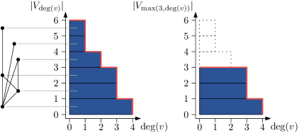
Figure 6: Visualization of how the sum over the degrees can be turned into an integral (left). The same visualization but only the degrees of vertices with degree at least $3$ are summed up (right).

To compute this integral, we first calculate the minimum and maximum degrees $k_{\min}$ and $k_{\max}$. Afterwards, we apply Lemma 4.7 to bound $|V_{x}^{S}|$. For the minimum degree $k_{\min}$, assume that vertex $v$ has radius $\rho_{O}=R-(2+\varepsilon)\log\log(n)$ for any constant $\varepsilon\in(0,1)$. Using Equation (4) the expected degree of $v$ is

$$\mathbb{E}[\deg(v)]=\Theta(ne^{-R/2+(1+\varepsilon/2)\log\log(n)})=\Theta(\log(n)^{1+\varepsilon/2}).$$

Since $\varepsilon>0$, this bound is $\omega(\log n)$, allowing us to apply the Chernoff-Hoeffding bounds in Corollaries 2.4 and 2.6 to conclude that $\deg(v)=\Theta(\log(n)^{1+\varepsilon/2})$ with high probability. Note that this only holds under the assumption that $v$ has radius exactly $\rho_{O}$. However, by Lemma 2.1 all vertices with smaller radius have larger expected degree. Therefore, $\Theta(\log(n)^{1+\varepsilon/2})$ is a lower bound on the expected degrees of all such vertices, allowing us to apply Corollary 2.6 together with a union bound, to conclude that, with high probability, no vertex with smaller radius has smaller degree. Thus, with high probability, the minimum degree in $S|_{\rho_{I}(\varphi^{\prime})}^{\rho_{O}}$ is $k_{\min}=\Theta(\log(n)^{1+\varepsilon/2})$. Analogously, the bound on the maximum degree $k_{\max}$ of a vertex in $S|_{\rho_{I}(\varphi^{\prime})}^{\rho_{O}}$ can be obtained as follows. Let $v$ be a vertex with radius $\rho_{I}(\varphi^{\prime})=R-1/\alpha(\log(\varphi^{\prime}/2\pi)+\log n-\log\log n)$. The expected degree of $v$ is $\mathbb{E}[\deg(v)]=\Theta((\varphi^{\prime}n/\log n)^{1/(2\alpha)})$ (Equation (4)). Since $\varphi^{\prime}=2\varphi\in\Omega(\log(n)^{2\alpha+1}/n)$, which is a precondition of this lemma, we can conclude that this bound on the expected degree of $v$ is $\Omega(\log n)$, allowing us to apply Corollary 2.4 to conclude that $\mathbb{E}[\deg(v)]=\mathcal{O}((\varphi n/\log n)^{1/(2\alpha)})$ holds with high probability. Again, this only holds under the assumption that $v$ has radius exactly $\rho_{I}(\varphi^{\prime})$. However, by Lemma 2.1 all vertices with larger radius have smaller expected degree. Therefore, $\mathcal{O}((\varphi n/\log n)^{1/(2\alpha)})$ is a valid upper bound on all their expected degrees, allowing us to apply Corollary 2.4 together with a union bound, to conclude that no vertex with larger radius has larger degree. Thus, the maximum degree in $S|_{\rho_{I}(\varphi^{\prime})}^{\rho_{O}}$ is $k_{\max}=\mathcal{O}((\varphi n/\log n)^{1/(2\alpha)})$ with high probability.

Using Lemma 4.7 we obtain $|V_{x}^{S}|=\mathcal{O}(\varphi nx^{-2\alpha})$ with probability $1-\mathcal{O}(n^{-c})$ for any constant $c>0$. Note that the requirements $x=\omega(\log n)$ and $x=\mathcal{O}((\varphi n/\log n)^{1/(2\alpha)})$ in Lemma 4.7 are satisfied as $k_{\min}\leq x\leq k_{\max}$. By choosing $c=2$ and applying the union bound over all degrees, we can conclude that, with high probability

$$\sum_{v\in S|_{\rho_{I}(\varphi^{\prime})}^{\rho_{O}}}\deg(v) =\mathcal{O}(\varphi nk_{\min}^{-(2\alpha-1)})+\mathcal{O}(\varphi n\cdot\int_{k_{\min}}^{k_{\max}}x^{-2\alpha}\operatorname{d\!}x)$$

$$=\mathcal{O}(\varphi nk_{\min}^{-(2\alpha-1)})+\mathcal{O}(\varphi n\cdot k_{\min}^{-(2\alpha-1)}(1-(k_{\min}/k_{\max})^{2\alpha-1})).$$

As $k_{\min}\leq k_{\max}$, this can be further simplified to $\mathcal{O}(\varphi nk_{\min}^{-(2\alpha-1)})$, which is $\mathcal{O}(\varphi n)$ since $k_{\min}=\omega(\log n)$.

It remains to bound the sum of the degrees of vertices in the central part of the disk $D_{R}|_{\rho_{I}(2\pi)}^{\rho_{O}}$ that lie in the neighborhood of a vertex $v$ with radius $\rho$, i.e., vertices lying in $D_{R}(v)$. Similar to the bounds for a sector $S$, we bound the sum of degrees in $D_{R}(v)$ by bounding the number of vertices with a fixed degree $k$ for every possible value of $k$. If all these bounds hold with probability $1-\mathcal{O}(n^{-3})$, then the union bound shows that the sum is concentrated with probability $1-\mathcal{O}(n^{-2})$. To obtain a bound that holds for every possible angular coordinate of $v$ (as claimed in Section 3.3.2), we apply Lemma 2.8. There, we choose the random variables $X_{w}$ to represent the degrees of the vertices. Our bound on the sum that holds with probability $1-\mathcal{O}(n^{-2})$ at a fixed angular coordinate, can then be translated to the same asymptotic bound that holds with probability $1-\mathcal{O}(n^{-1})$ at every possible angular coordinate.

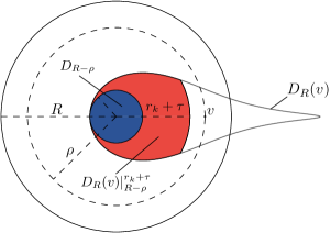
Figure 7: Determining the sum of degrees of the neighbors of vertex $v$ that are all contained in $D_{R}(v)$. To compute the measure of $D_{R}(v)|_{0}^{r_{k}+\tau}$ we divide it into two regions $D_{R}(v)|_{0}^{R-\rho}=D_{R-\rho}$ (blue) and $D_{R}(v)|_{R-\rho}^{r_{k}+\tau}$ (red).

For a fixed degree $k=\omega(\log n)$, all vertices with degree at least $k$ have radius at most $r_{k}+\tau$ with high probability due to Lemma 4.5, where $r_{k}=2\log(n/k)$ and $\tau$ is constant. Thus, all vertices of degree at least $k$ in $D_{R}(v)$ lie in $D_{R}(v)|_{0}^{r_{k}+\tau}$, with high probability. In analogy to Lemma 4.7, we obtain the following bound on the number of vertices in $D_{R}(v)|_{0}^{r_{k}+\tau}$.

Lemma 4.11.

Let $G$ be a hyperbolic random graph and let $v$ be a vertex with radius $\rho=1/\alpha(\log n-\log\log n)$. If $k=\omega(\log n)$, the number of neighbors of $v$ with degree at least $k$ is

$$|\{w\in N(v)\mid\deg(w)\geq k\}|=\mathcal{O}(n^{1-1/(2\alpha)}\log(n)^{1/(2\alpha)}k^{-(2\alpha-1)}+\log n)$$

with probability $1-\mathcal{O}(n^{-c})$ for any constant $c>0$.

Proof 4.12.

Since $k=\omega(\log n)$, we can apply Lemma 4.5 stating that all vertices of degree at least $k$ in $D_{R}(v)$ lie within $D_{R}(v)|_{0}^{r_{k}+\tau}$ with high probability. To bound the number of neighbors of $v$ with degree at least $k$ we first compute the measure $\mu(D_{R}(v)|_{0}^{r_{k}+\tau})$. To do this, we separate $D_{R}(v)|_{0}^{r_{k}+\tau}$ into the disk $D_{R}(v)|_{0}^{R-\rho}=D_{R-\rho}$ and $D_{R}(v)|_{R-\rho}^{r_{k}+\tau}$; see Figure 7. Due to Equation (3), we have $\mu(D_{R-\rho})=\mathcal{O}(e^{-\alpha(R-(R-\rho))})=\mathcal{O}(\log n/n)$, which is already an upper bound on $\mu(D_{R}(v)|_{0}^{r_{k}+\tau})$ for the case where $r_{k}+\tau\leq R-\rho$. When $r_{k}+\tau>R-\rho$, we need to add the measure of $D_{R}(v)|_{R-\rho}^{r_{k}+\tau}$, which is given by

$$\mu(D_{R}(v)|_{R-\rho}^{r_{k}+\tau})=\int_{R-\rho}^{r_{k}+\tau}2\int_{0}^{\theta(\rho,r)}f(r,\phi)\operatorname{d\!}\phi\operatorname{d\!}r=\mathcal{O}\left(\int_{R-\rho}^{r_{k}+\tau}\theta(\rho,r)f(r)\operatorname{d\!}r\right)$$

Since we consider $r\in[R-\rho,r_{k}+\tau]$ in the integral, we have $r\geq R-\rho$, allowing us to apply Equation (2.2) to conclude that $\theta(\rho,r)=\mathcal{O}(e^{(R-\rho-r)/2})$. Furthermore, we can substitute the probability density $f(r)=\mathcal{O}(e^{-\alpha(R-r)})$ (Equation (1)) to obtain

$$\mu(D_{R}(v)|_{R-\rho}^{r_{k}+\tau}) =\mathcal{O}\left(\int_{R-\rho}^{r_{k}+\tau}e^{(R-\rho-r)/2}\cdot e^{-\alpha(R-r)}\operatorname{d\!}r\right)$$

$$=\mathcal{O}\left(e^{(R-\rho)/2}\cdot e^{-\alpha R}\cdot\int_{R-\rho}^{r_{k}+\tau}e^{(\alpha-1/2)r}\operatorname{d\!}r\right)$$

$$=\mathcal{O}\left(e^{-(\alpha-1/2)R}\cdot e^{-\rho/2}\cdot\left[e^{(\alpha-1/2)(r_{k}+\tau)}-e^{(\alpha-1/2)(R-\rho)}\right]\right).$$

Dropping the negative term in the brackets and substituting $R=2\log n+C$, $\rho=1/\alpha(\log n-\log\log n)$, and $r_{k}=2\log(n/k)$, we obtain

$$\mu(D_{R}(v)|_{R-\rho}^{r_{k}+\tau}) =\mathcal{O}\left(e^{-(\alpha-1/2)R}\cdot e^{-\rho/2}\cdot e^{(\alpha-1/2)(r_{k}+\tau)}\right)$$

$$=\mathcal{O}\left(n^{-(2\alpha-1)}\cdot n^{-1/(2\alpha)}\log(n)^{1/(2\alpha)}\cdot n^{2\alpha-1}\cdot k^{-(2\alpha-1)}\right)$$

$$=\mathcal{O}\left((\log(n)/n)^{1/(2\alpha)}\cdot k^{-(2\alpha-1)}\right).$$

The expected number of vertices in $D_{R}(v)|_{0}^{r_{k}+\tau}$ is now obtained by reversing the previous split and adding the measures of $D_{R-\rho}$ and $D_{R}(v)|_{R-\rho}^{r_{k}+\tau}$, which yields

$$\mathbb{E}[|\{v\in D_{R}(v)|_{0}^{r_{k}+\tau}\}|] =n\cdot\left(\mu(D_{R-\rho})+\mu(D_{R}(v)|_{R-\rho}^{r_{k}+\tau})\right)$$

$$=\mathcal{O}(\log n+n^{1-1/(2\alpha)}\log(n)^{1/(2\alpha)}k^{-(2\alpha-1)})$$

and it remains to show that this bound holds with large enough probability. Clearly, this bound is at least logarithmic. Thus, we can apply Corollary 2.4 to conclude that it holds with probability $1-\mathcal{O}(n^{-c})$ for any constant $c$.

With this, we are now ready to bound the sum of the degrees of the vertices in the central part of the disk that are in the neighborhood of a vertex with radius $\rho$. The proof of the following lemma is analogous to the one of Lemma 4.9.

Lemma 4.13.

Let $G$ be a hyperbolic random graph and let $v$ be a hypothetical vertex with radius $\rho=1/\alpha(\log n-\log\log n)$ and arbitrary angular coordinate. The degrees of neighbors of $v$ in $D_{R}|_{\rho_{I}(2\pi)}^{\rho_{O}}$ sum to $\mathcal{\tilde{O}}(n^{1/(2\alpha)})$ with high probability.

Proof 4.14.

Recall that $D_{R}(v)$ is the disk containing all neighbors of $v$. To bound the sum of the degrees of the vertices in $D_{R}(v)|_{\rho_{I}(2\pi)}^{\rho_{O}}$, we use basically the same proof as in Lemma 4.9 except we use Lemma 4.11 instead of Lemma 4.7. Thus,

$$\sum_{w\in D_{R}(v)|_{\rho_{I}(2\pi)}^{\rho_{O}}}\deg(w) \leq k_{\min}|V_{k_{\min}}^{D_{R}(v)}|+\int_{k_{\min}}^{k_{\max}}|V_{x}^{D_{R}(v)}|\operatorname{d\!}x,$$

where $V_{x}^{D_{R}(v)}$ is the set of vertices of degree at least $x$ in $D_{R}(v)$ and $k_{\min}$ and $k_{\max}$ are the maximum and minimum degree in $D_{R}(v)|_{\rho_{I}(2\pi)}^{\rho_{O}}$, respectively.

We start with computing $k_{\min}$ and $k_{\max}$. Using Equation (4) and Corollaries 2.4 and 2.6, we obtain that a vertex of radius $\rho_{O}=R-(2+\varepsilon)\log\log n$, for any $\varepsilon\in(0,1)$, has degree $k_{\min}=\Theta((\log n)^{1+\varepsilon/2})$ with high probability. Moreover, by the same argumentation as in the proof of Lemma 4.9 no vertex with smaller radius has smaller degree, with high probability. Additionally, a vertex with radius $\rho_{I}(2\pi)=R-1/\alpha(\log n-\log\log n)$ has degree $k_{\max}=\mathcal{O}((n/\log n)^{1/(2\alpha)})$ and no vertex with larger radius has larger degree, with high probability. It follows that we can use the bound shown in Lemma 4.11 for $|V_{x}^{D_{R}(v)}|$. Thus, we obtain

$$\sum_{w\in D_{R}(v)|_{\rho_{I}(2\pi)}^{\rho_{O}}}\deg(w) =\mathcal{\tilde{O}}\big{(}k_{\min}\cdot n^{1-1/(2\alpha)}k_{\min}^{-(2\alpha-1)}\big{)}+\mathcal{\tilde{O}}\big{(}n^{1-1/(2\alpha)}\int_{k_{\min}}^{k_{\max}}x^{-(2\alpha-1)}\operatorname{d\!}x\big{)}.$$

Replacing $k_{\min}$ and simplifying the first term in the sum yields $\mathcal{\tilde{O}}(n^{1-1/(2\alpha)})$, which is smaller than the claimed bound. For the second term, we obtain

$$\mathcal{\tilde{O}}\left(n^{1-1/(2\alpha)}\int_{k_{\min}}^{k_{\max}}x^{-(2\alpha-1)}\operatorname{d\!}x\right) =\mathcal{\tilde{O}}\left(n^{1-1/(2\alpha)}\left[k_{\max}^{2-2\alpha}-k_{\min}^{2-2\alpha}\right]\right).$$

Dropping the negative term and replacing $k_{\max}=\mathcal{\tilde{O}}(n^{1/(2\alpha)})$, we obtain $\mathcal{\tilde{O}}(n^{1-1/(2\alpha)+1/\alpha-1})=\mathcal{\tilde{O}}(n^{1/(2\alpha)})$.

4.3 The Outer Part of the Disk

At this point we have bounded the sum of the degrees of the vertices with radius at most $\rho_{O}=R-(2+\varepsilon)\log\log n$ (for any constant $\varepsilon\in(0,1)$) that lie in a sector of angular width $\varphi\in\Omega(\log(n)^{2\alpha+1}/n)$ or in the neighborhood of a vertex with radius $\rho$. It remains to bound the sums when considering vertices with radii larger than $\rho_{O}$.

To bound the sum of the vertex degrees in the outer part of a sector $S|_{\rho_{O}}^{R}$, we start by computing the expected value.

Lemma 4.15.

Let $G$ be a hyperbolic random graph. For a sector $S$ of angular width $\varphi$, the degrees of vertices in $S|_{\rho_{O}}^{R}$ sum to $\Theta(\varphi n)$ in expectation.

Proof 4.16.

Let $\deg(v)$ be the random variable describing the degree of a vertex $v$. Moreover, let $X_{v}$ be the indicator variable that is $1$ if $v\in S|_{\rho_{O}}^{R}$ and $0$ otherwise. Then the expected sum of the degrees of vertices in $S|_{\rho_{O}}^{R}$ is given by

$$\mathbb{E}\left[\sum_{v\in V}X_{v}\cdot\deg(v)\right]=\sum_{v\in V}\mathbb{E}[X_{v}\cdot\deg(v)]=n\cdot\Pr[v\in S|_{\rho_{O}}^{R}]\cdot\mathbb{E}[\deg(v)\mid v\in S|_{\rho_{O}}^{R}].$$

Note that $\Pr[v\in S|_{\rho_{O}}^{R}]$ is simply the measure $\mu(S|_{\rho_{O}}^{R})$. As the angular coordinate is uniformly distributed, the whole sector $S$ has measure $\Theta(\varphi)$. Moreover, the region of the disk containing the points with constant distance to the boundary has constant measure. Thus, the measure of $S|_{\rho_{O}}^{R}$ is also in $\Theta(\varphi)$. For the sake of completeness, the measure of $S|_{\rho_{O}}^{R}$ can be formally computed as

$$\mu(S|_{\rho_{O}}^{R}) =\mu(S\setminus S|_{0}^{\rho_{O}})$$

$$=\frac{\varphi}{2\pi}(1-\mu(D_{\rho_{O}}))$$

$$=\frac{\varphi}{2\pi}(1-e^{-\alpha(R-\rho_{O})}(1+o(1)))$$

$$=\frac{\varphi}{2\pi}(1-\mathcal{O}((\log n)^{-\alpha(2+\varepsilon)}))$$

$$=\Theta(\varphi).$$

It remains to determine $\mathbb{E}[\deg(v)\leavevmode\nobreak\ |\leavevmode\nobreak\ v\in S|_{\rho_{O}}^{R}]$, which can be done as follows.

$$\mathbb{E}[\deg(v)\mid v\in S|_{\rho_{O}}^{R}] =\iint_{S|_{\rho_{O}}^{R}}\mathbb{E}[\deg(v)\leavevmode\nobreak\ |\leavevmode\nobreak\ r(v)=r]\frac{f(r,\phi)}{\mu(S|_{\rho_{O}}^{R})}\operatorname{d\!}\phi\operatorname{d\!}r$$

$$=\frac{1}{\mu(S|_{\rho_{O}}^{R})}\cdot\int_{\rho_{O}}^{R}\int_{0}^{\varphi}\mathbb{E}[\deg(v)\leavevmode\nobreak\ |\leavevmode\nobreak\ r(v)=r]f(r,\phi)\operatorname{d\!}\phi\operatorname{d\!}r$$

$$=\Theta(1)\cdot\int_{\rho_{O}}^{R}\mathbb{E}[\deg(v)\leavevmode\nobreak\ |\leavevmode\nobreak\ r(v)=r]f(r)\operatorname{d\!}r$$

$$=\Theta(1)\cdot n\cdot e^{-\alpha R}\int_{\rho_{O}}^{R}e^{(\alpha-1/2)r}\operatorname{d\!}r$$

$$=\Theta(1)\cdot n\cdot e^{-\alpha R}\left[e^{(\alpha-1/2)R}-e^{(\alpha-1/2)\rho_{O}}\right]$$

$$=\Theta(1)\cdot n\cdot e^{-R/2}\left[1-e^{-(\alpha-1/2)(R-\rho_{O})}\right]$$

Note that the part in brackets is bounded by a constant. Moreover, as $R=2\log n+C$, $n\cdot e^{-R/2}$ is constant as well. Thus, $\mathbb{E}[\deg(v)\mid v\in S|_{\rho_{O}}^{R}]$ is in $\Theta(1)$. It follows that the expected sum of the degrees is $\Theta(\varphi n)$.

Unfortunately, the sum of the vertex degrees in $S|_{\rho_{O}}^{R}$ is not concentrated sufficiently well around its expectation to conclude that this bound also holds with high probability. The problem lies with the high-degree vertices in the graph, which can be adjacent to none or all vertices in $S|_{\rho_{O}}^{R}$ depending on their positions. That is, small perturbations of the position of a single high-degree vertex can change the sum by too much. To overcome this issue, we consider the impact of high-degree vertices separately. To this end, we partition the edge set that contributes to the degrees of the vertices in $S|_{\rho_{O}}^{R}$ into two sets $E_{I}$ and $E_{O}$, denoting the inner edges where the other endpoint is in $D_{R}|_{0}^{\rho_{O}}$ and the outer edges where the other endpoint is in $D_{R}|_{\rho_{O}}^{R}$. The sum of the degrees of the vertices in $S|_{\rho_{O}}^{R}$ can then be bounded by taking the number of inner edges and adding them to twice the number of outer edges. That is,

$$\sum_{v\in S|_{\rho_{O}}^{R}}\deg(v)\leq|E_{I}|+2|E_{O}|.$$

Since $E_{I}$ denotes all edges with one endpoint in $S|_{\rho_{O}}^{R}$ and the other in the inner or central part of the disk, we can obtain an upper bound on the first summand by summing the degrees of the vertices in $D_{R}|_{0}^{\rho_{O}}$ that are adjacent to any vertex in $S|_{\rho_{O}}^{R}$. Since $\rho\leq\rho_{O}$, we have $S|_{\rho_{O}}^{R}\subseteq S|_{\rho}^{R}$, allowing us to apply Lemma 3.10 to conclude that all such vertices are contained in $S$ or are neighbors of the two hypothetical corner vertices $c_{1}$ and $c_{2}$, which both have radius $\rho$. Thus, $|E_{I}|$ can be bounded by the sum of the degrees of vertices in a sector and in the neighborhood of a vertex with radius $\rho$, but constrained to vertices in the inner and central parts of the disk. Corresponding bounds that hold with high probability have been determined above. For the sector we obtain an upper bound of $\mathcal{\tilde{O}}(\delta_{\max})$ for the inner part (Corollary 4.3) and $\mathcal{O}(\varphi n)$ for the central part (Lemma 4.9). For the neighborhood of a vertex with radius $\rho$ we have $\mathcal{\tilde{O}}(\delta_{\max})$ for the inner part (Corollary 4.4) and $\mathcal{\tilde{O}}(n^{1/(2\alpha)})$ for the central part (Lemma 4.13). Taking them together, we obtain the following corollary.

Corollary 4.17.

Let $G$ be a hyperbolic random graph. For every sector $S$ of angular width $\varphi\in\Omega(\log(n)^{2\alpha+1}/n)$, the number of edges with one endpoint in $S|_{\rho_{O}}^{R}$ and the other in $D_{R}|_{0}^{\rho_{O}}$ is in $\mathcal{\tilde{O}}(\varphi n+n^{1/(2\alpha)}+\delta_{\max})$, with high probability.

To obtain an upper bound on the second part of the above sum, we aim to apply a method of typical bounded differences based on the fact that changing the position of a single vertex has typically only little impact on the number of outer edges. The idea is as follows. We consider $|E_{O}|$ as a function that only depends on the positions $P_{1},\dots,P_{n}$ of the vertices in the graph and we ask ourselves: How much can $|E_{O}|$ change, if we alter the position of a single vertex $i$? Clearly, this change can be large in the worst case. Assume that we move $i$ from outside $D_{R}|_{\rho_{O}}^{R}$ into $S|_{\rho_{O}}^{R}$. Then, $i$ does not contribute anything to $|E_{O}|$ before the move and the increase in $|E_{O}|$ depends on the number of outer edges that are incident to $i$ after the move, which can be $n-1$ in the worst case. However, it is very unlikely that a vertex in $S|_{\rho_{O}}^{R}$ has this many neighbors that lie in the outer part of the disk. In fact, its degree is typically much smaller. To formalize this, we represent the typical case using an event $A$, denoting that the degree of such a vertex is at most a constant factor larger than the expected degree of a vertex with radius $\rho_{O}=R-(2+\varepsilon)\log\log n$ for any constant $\varepsilon\in(0,1)$. More precisely, $A$ denotes the event in which all disks of radius $R$ with center in $D_{R}|_{\rho_{O}}^{R}$ contain at most $\mathcal{O}(\log(n)^{1+\varepsilon/2})$ vertices. In this case, moving a vertex $i$ in the same way as before leads to a much smaller increase in the number of outer edges. Assuming that $A$ holds before the move, there are at most $\mathcal{O}(\log(n)^{1+\varepsilon/2})$ outer edges incident to $i$ after the move, which corresponds to the increase of $|E_{O}|$. The following lemma defines the event $A$ formally and shows that it holds with high probability.

Lemma 4.18.

Let $G$ be a hyperbolic random graph and let $\rho_{O}=R-(2+\varepsilon)\log\log(n)$ for any constant $\varepsilon\in(0,1)$. Then, all disks $D$ with radius $R$ and center in $D_{R}|_{\rho_{O}}^{R}$ contain at most $|\{v\in D\}|=\mathcal{O}(\log(n)^{1+\varepsilon/2})$ vertices, with probability $1-\mathcal{O}(n^{-c})$ for any constant $c$.

Proof 4.19.

Let $D$ be a disk of radius $R$ and center $P\in D_{R}|_{\rho_{O}}^{R}$. By Lemma 2.1, a valid upper bound on the expected number of vertices in $D$ can be obtained by considering the disk $D^{\prime}$ at center $P^{\prime}$ instead, which has the same angular coordinate as $P$ and radius $\rho_{O}$. Thus, using Lemma (4) we get

$$\mathbb{E}[|\{v\in D\}|]\leq\mathbb{E}[|\{v\in D^{\prime}\}|]=\mathcal{O}(ne^{-\rho_{O}/2})=\mathcal{O}(\log(n)^{1+\varepsilon/2}).$$

Moreover, since $\varepsilon>0$, this bound is $\omega(\log n)$ and we can apply Corollary 2.4 to conclude that $|\{v\in D\}|\in\mathcal{O}(\log(n)^{1+\varepsilon/2})$ holds with probability $1-\mathcal{O}(n^{-c^{\prime}})$ for any constant $c^{\prime}$. To obtain a bound that holds for every possible angular coordinate for $P$, we apply Lemma 2, which allows us to translate our bound that holds for any given disk $D$ with probability $1-\mathcal{O}(n^{-c^{\prime}})$ to the same asymptotic bound that holds with probability $1-\mathcal{O}(n^{-c^{\prime}+1})$ for all possible angular coordinates. Choosing $c^{\prime}=c+1$ then yields the claim.

So while moving a single vertex leads to a large change in the number of outer edges $|E_{O}|$ in the worst case, we observe only small changes in the typical case $A$. Formally, we say that a function $f\colon\Omega^{n}\rightarrow\mathbb{R}$ satisfies the typical bounded differences condition with respect to an event $A\subseteq\Omega^{n}$ if for all $i\in\{1,\dots,n\}$ there exist $\Delta_{i}^{A}\leq\Delta_{i}$ such that

$$|f(\boldsymbol{x})-f(\boldsymbol{x}^{\prime})|\leq\begin{cases}\Delta_{i}^{A},&\text{if}\leavevmode\nobreak\ \boldsymbol{x}\in A,\\ \Delta_{i},&\text{otherwise},\end{cases}$$

for all $\boldsymbol{x},\boldsymbol{x}^{\prime}\in\Omega^{n}$ that differ only in the $i$th component.

Theorem 4.20 (Method of Typical Bounded Differences, [27, Theorem 2]).

Let $X_{1},\dots,X_{n}\in\Omega$ be independent random variables and let $A\subseteq\Omega^{n}$ be an event. Furthermore, let $f\colon\Omega^{n}\rightarrow\mathbb{R}$ be a function that satisfies the typical bounded differences condition with respect to $A$ and with parameters $\Delta_{i}^{A}\leq\Delta_{i}$ for $i\in\{1,\dots,n\}$. Then for all $\varepsilon_{1},\dots,\varepsilon_{n}\in(0,1]$ there exists an event $B$ satisfying $\bar{B}\subseteq A$ and $\Pr[B]\leq\Pr[\bar{A}]\cdot\sum_{i}1/\varepsilon_{i}$, such that for $\Delta=\sum_{i}(\Delta_{i}^{A}+\varepsilon_{i}(\Delta_{i}-\Delta_{i}^{A}))^{2}$ and $t\geq 0$ it holds that

$$\Pr[f>\mathbb{E}[f]+t\land\bar{B}]\leq e^{-t^{2}/(2\Delta)}.$$

Intuitively, the choice of the values for $\varepsilon_{i}$ has two effects. On the one hand, choosing $\varepsilon_{i}$ small allows us to compensate for a potentially large worst-case change $\Delta_{i}$. On the other hand, this also increases the bound on the probability of the event $B$ that represents the atypical case. However, in that case one can still obtain meaningful bounds if the typical event $A$ occurs with high enough probability. In the following, we show that an upper bound on the expected value $\mathbb{E}[f]$ is sufficient to apply the method of typical bounded differences, before applying it to bound the number of outer edges in a sector.

Corollary 4.21.

Let $X_{1},\dots,X_{n}\in\Omega$ be independent random variables and let $A\subseteq\Omega^{n}$ be an event. Furthermore, let $f\colon\Omega^{n}\rightarrow\mathbb{R}$ be a function that satisfies the typical bounded differences condition with respect to $A$ and with parameters $\Delta_{i}^{A}\leq\Delta_{i}$ for $i\in\{1,\dots,n\}$ and let $g(n)$ be an upper bound on $\mathbb{E}[f]$. Then for all $\varepsilon_{1},\dots,\varepsilon_{n}\in(0,1]$, $\Delta=\sum_{i}(\Delta_{i}^{A}+\varepsilon_{i}(\Delta_{i}-\Delta_{i}^{A}))^{2}$, and $c\geq 1$ it holds that

$$\Pr[f>cg(n)]\leq e^{-((c-1)g(n))^{2}/(2\Delta)}+\Pr[\bar{A}]\sum_{i}1/\varepsilon_{i}.$$

Proof 4.22.

Let $h(n)\geq 0$ be a function with $f^{\prime}=f+h(n)$ such that $\mathbb{E}[f^{\prime}]=g(n)$. Note that $h(n)$ exists since $g(n)\geq\mathbb{E}[f]$. As a consequence, we have $f\leq f^{\prime}$ for all outcomes of $X_{1},\dots,X_{n}$ and it holds that

$$|f^{\prime}(\boldsymbol{x})-f^{\prime}(\boldsymbol{x}^{\prime})|=|f(\boldsymbol{x})+h(n)-f(\boldsymbol{x}^{\prime})-h(n)|=|f(\boldsymbol{x})-f(\boldsymbol{x}^{\prime})|,$$

for all $\boldsymbol{x},\boldsymbol{x}^{\prime}\in\Omega^{n}$. Consequently, $f^{\prime}$ satisfies the typical bounded differences condition with respect to $A$ with the same parameters $\Delta_{i}^{A}\leq\Delta_{i}$ as $f$. Since $f\leq f^{\prime}$ it holds that

$$\Pr[f>cg(n)]\leq\Pr[f^{\prime}>cg(n)]=\Pr[f^{\prime}>c\mathbb{E}[f^{\prime}]].$$

By choosing $t=(c-1)\mathbb{E}[f^{\prime}]$ this can be written as

$$\Pr[f^{\prime}>c\mathbb{E}[f^{\prime}]]=\Pr[f^{\prime}>\mathbb{E}[f^{\prime}]+t].$$

Theorem 4.20 now guarantees the existence of an event $B$ with $\Pr[B]\leq\Pr[\bar{A}]\cdot\sum_{i}1/\varepsilon_{i}$ and $\bar{B}\subseteq A$, such that $\Pr[f^{\prime}>\mathbb{E}[f^{\prime}]+t\land\bar{B}]\leq e^{-t^{2}/(2\Delta)}$. To bound $\Pr[f^{\prime}>\mathbb{E}[f^{\prime}]+t]$ we apply the law of total probability and consider the events $B$ and $\bar{B}$ separately

$$\Pr[f^{\prime}>\mathbb{E}[f^{\prime}]+t]=\Pr[f^{\prime}>\mathbb{E}[f^{\prime}]+t\mid\bar{B}]\cdot\Pr[\bar{B}]+\Pr[f^{\prime}>\mathbb{E}[f^{\prime}]+t\mid B]\cdot\Pr[B].$$

The first part of the sum can be simplified using the definition of conditional probabilities. Moreover, it holds that $\Pr[f^{\prime}>\mathbb{E}[f^{\prime}]+t\mid B]\leq 1$. Thus, we can bound the above term by

$$\Pr[f^{\prime}>\mathbb{E}[f^{\prime}]+t]\leq\Pr[f^{\prime}>\mathbb{E}[f^{\prime}]+t\land\bar{B}]+\Pr[B].$$

Both remaining summands can now be bounded using the upper bounds that we previously obtained by applying Theorem 4.20, i.e., $\Pr[f^{\prime}>\mathbb{E}[f^{\prime}]+t\land\bar{B}]\leq e^{-t^{2}/(2\Delta)}$ and $\Pr[B]\leq\Pr[\bar{A}]\cdot\sum_{i}1/\varepsilon_{i}$. Thus,

$$\Pr[f^{\prime}>\mathbb{E}[f^{\prime}]+t]\leq e^{-t^{2}/(2\Delta)}+\Pr[\bar{A}]\cdot\sum_{i}1/\varepsilon_{i}.$$

Finally, since $t$ was chosen as $t=(c-1)\mathbb{E}[f^{\prime}]$ and since $\mathbb{E}[f^{\prime}]=g(n)$, we obtain the claimed bound.

We are now ready to bound the number $|E_{O}|$ of outer edges, i.e, edges that are incident to vertices in a sector $S|_{\rho_{O}}^{R}$ and have their other endpoint in $D_{R}|_{\rho_{O}}^{R}$.

Lemma 4.23.

Let $G$ be a hyperbolic random graph. For every sector $S$ of angular width $\varphi\in\Omega(\log(n)^{2}/n^{1/2})$, the number of edges with one endpoint in $S|_{\rho_{O}}^{R}$ and the other in $D_{R}|_{\rho_{O}}^{R}$ is in $\mathcal{O}(\varphi n)$, with high probability.

Proof 4.24.

First note that, analogous to the proof of Lemma 4.9, we can cover the disk with $\mathcal{O}(n)$ sectors of angular width $2\varphi$ such that any sector of angular width $\varphi$ lies completely in one of them. In the following, we show that the claimed bound holds with probability $\mathcal{O}(n^{-2})$ for a single sector $S$ of twice the width. Applying union bound then yields the claim.

We consider $|E_{O}|$, the number of edges with one endpoint in $S|_{\rho_{O}}^{R}$ and the other in $D_{R}|_{\rho_{O}}^{R}$, as a function hat only depends on the positions $P_{1},\dots,P_{n}$ of the vertices in the graph. To show that $|E_{O}|$ does not exceed an upper bound with high probability, we aim to apply the method of typical bounded differences (Corollary 4.21). We represent the typical case with an event $A$, denoting that all disks $D$ of radius $R$ and center in $D_{R}|_{\rho_{O}}^{R}$ contain at most $\mathcal{O}(\log(n)^{1+\varepsilon/2})$ vertices for any constant $\varepsilon\in(0,1)$. In order to determine the parameters $\Delta_{i}^{A}\leq\Delta_{i}$ for $i\in\{1,\dots,n\}$ with which $|E_{O}|$ fulfills the typical bounded differences condition with respect to $A$, we have to bound the maximum change in $|E_{O}|$ obtained by moving a single vertex. As argued before, this change is at most $\Delta_{i}=n-1$ for all $i\in\{1,\dots,n\}$ in the worst case. To bound the $\Delta_{i}^{A}$, we start with a configuration of vertex coordinates in which the event $A$ holds. In this case, it is easy to see that moving a single vertex $i$ changes $|E_{O}|$ by at most $\Delta_{i}^{A}=\mathcal{O}(\log(n)^{1+\varepsilon/2})$ for all $i\in\{1,\dots,n\}$, since the degree of $i$ is at most this large after the move and so is the number of outer edges it contributes to $|E_{O}|$.

We are now ready to apply the method of typical bounded differences (Corollary 4.21). For an upper bound $g(n)$ on $|E_{O}|$, any constant $c>1$, and all $\varepsilon_{1},\dots,\varepsilon_{n}\in(0,1]$ it states that

$$\Pr[|E_{O}|>cg(n)]\leq e^{-((c-1)g(n))^{2}/(2\Delta)}+\Pr[\bar{A}]\sum_{i}1/\varepsilon_{i},$$

where $\Delta=\sum_{i}(\Delta_{i}^{A}+\varepsilon_{i}(\Delta_{i}-\Delta_{i}^{A}))^{2}$. First note that a valid upper bound on the expected number of outer edges incident to vertices in $S|_{\rho_{O}}^{R}$ is given by the expected sum of the degrees of these vertices. Thus, by Lemma 4.15 we can choose $g(n)=\Theta(\varphi n)$. Moreover, by choosing $\varepsilon_{i}=1/n$ for all $i\in\{1,\dots,n\}$ and since $\Delta_{i}=n-1$ and $\Delta_{i}^{A}=\mathcal{O}(\log(n)^{1+\varepsilon/2})$ for all $i\in\{1,\dots,n\}$, we can compute $\Delta$ as

$$\Delta =\sum_{i}(\Delta_{i}^{A}+\varepsilon_{i}(\Delta_{i}-\Delta_{i}^{A}))^{2}$$

$$=\mathcal{O}\left(n\cdot\left(\log(n)^{1+\varepsilon/2}+1/n(n-\log(n)^{1+\varepsilon/2})\right)^{2}\right)$$

$$=\mathcal{O}\left(n\cdot\left(\log(n)^{1+\varepsilon/2}+(1-o(1))\right)^{2}\right)$$

$$=\mathcal{O}\left(n\cdot\log(n)^{2+\varepsilon}\right)$$

Consequently, the above probability can be bounded by

$$\Pr[|E_{O}|>cg(n)] \leq\exp\left(-\Theta\left(\frac{(\varphi n)^{2}}{n\log(n)^{2+\varepsilon}}\right)\right)+\Pr[\bar{A}]\cdot n^{2}$$

$$\leq\exp\left(-\Theta\left(\frac{\varphi^{2}n}{\log(n)^{2+\varepsilon}}\right)\right)+\Pr[\bar{A}]\cdot n^{2}.$$

Since $\varphi\in\Omega(\log(n)^{2}/n^{1/2})$ is a precondition of this lemma and since $\varepsilon<1$, we can conclude that the fraction is $\omega(\log n)$, which means that the first summand is $\mathcal{O}(n^{-c^{\prime}})$ for any constant $c^{\prime}$. Moreover, by Lemma 4.18 event $A$ holds with probability $1-\mathcal{O}(n^{-c^{\prime}})$ for any constant $c^{\prime}$. Choosing $c^{\prime}=3$ then yields the claim.

4.4 The Complete Disk

Having obtained the required bounds for the inner, central, and outer parts of the disk, we can now combine them to bound the sum of the degrees in a sector and in the neighborhoods of the hypothetical corner vertices. We start with Theorem 3.8, which bounds the sum of degrees in a sector. To improve readability, we restate the theorem here.

Theorem 3.8.

Let $G$ be a hyperbolic random graph. The degrees of vertices in every sector of angular width $\varphi$ sum to $\mathcal{\tilde{O}}(\varphi n+n^{1/(2\alpha)}+\delta_{\max})$ with high probability if $\varphi=\Omega(\log(n)^{2}/n^{1/2}).$

Proof 4.25.

For the inner and central parts of every sector the sum of the vertex degrees is bounded by $\mathcal{\tilde{O}}(\varphi n+\delta_{\max})$ with high probability due to Corollary 4.3 and Lemma 4.9. As argued above, the sum of the degrees of the remaining vertices, i.e., vertices with radius at least $\rho_{O}$, can be bounded by counting the number of inner edges and adding twice the number of outer edges. Since $\varphi\in\Omega(\log(n)^{2}/n^{1/2})$, we can apply Corollary 4.17 and Corollary 4.23 to conclude that the corresponding sum is bounded by $\mathcal{\tilde{O}}(\varphi n+n^{1/(2\alpha)}+\delta_{\max})$, with high probability.

Lastly, it remains to bound the sum of the degrees of the neighbors of the hypothetical corner vertices that were used to bound the size of the search space in the second phase. Again, for the sake of readability, we restate the corresponding lemma here.

Lemma 3.14.

Let $G$ be a hyperbolic random graph and let $v$ be a hypothetical vertex with radius $\rho=1/\alpha(\log n-\log\log n)$ and arbitrary angular coordinate. The degrees of neighbors of $v$ sum to $\mathcal{\tilde{O}}(n^{2-1/\alpha}+n^{1/(2\alpha)}+\delta_{\max})$ with high probability.

Proof 4.26.

For the inner and central parts of the neighborhood of a vertex with radius $\rho$ and arbitrary angular coordinate the sum of the degrees is bounded by $\mathcal{\tilde{O}}(\delta_{\max}+n^{1/(2\alpha)})$ with high probability, due to Corollary 4.4 and Lemma 4.13. For the sum of the degrees in the outer part of the disk, note that all neighbors of radius at least $\rho$ have angular distance at most $\varphi=\mathcal{O}(n^{-(1/\alpha-1)})$; see Section 3.3.1. Thus, we can use Theorem 3.8 to conclude that claimed bound holds for the sum of their degrees. Note that if $\varphi$ is too small to meet the requirements of Theorem 3.8, we can choose $\varphi=\mathcal{\tilde{O}}(n^{-1/2})$ as a valid upper bound to conclude that the sum of degrees in the outer part of the neighborhood is in $\mathcal{\tilde{O}}(n^{1/2})$, which is $\mathcal{\tilde{O}}(n^{1/(2\alpha)})$ for $\alpha\in(1/2,1)$.

5 Conclusion

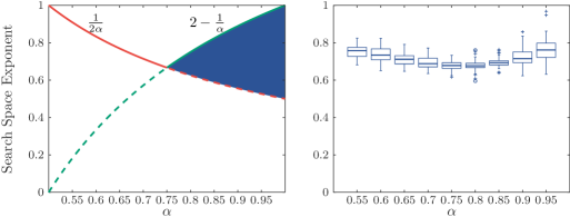
Figure 8: Left: The exponent of our theoretical bound depending on $\alpha$. Right: The corresponding empirically measured search spaces. The data was obtained by generating $20$ hyperbolic random graphs with average degree roughly $8$ for each shown $\alpha$ and each $n\in\{100$\mathrm{k}$,200$\mathrm{k}$,300$\mathrm{k}$\}$. For each graph we sampled $300$\mathrm{k}$$ start–destination pairs and report the maximum number of edges explored in one search. The numbers are normalized with the total number of edges $m$ of the graph such that $x$ is plotted for a search space of size $m^{x}$.

In the following, we briefly discuss why we think that the bound $\mathcal{\tilde{O}}(n^{2-1/\alpha}\allowbreak+n^{1/(2\alpha)}+\delta_{\max})$ is rather tight; see Figure 8 (left) for a plot of the exponents. Clearly, the maximum degree of the graph is a lower bound, i.e., we cannot improve the $\delta_{\max}$. As $\delta_{\max}=\tilde{\Theta}(n^{1/(2\alpha)})$ holds almost surely [17], we also cannot improve below $\mathcal{\tilde{O}}(n^{1/(2\alpha)})$. For the term $n^{2-1/\alpha}$ we do not have a lower bound. Thus, the blue region in Figure 8 (left) is the only part where our bound can potentially be improved. However, by only making a single step from a vertex with radius $\rho=1/\alpha(\log n-\log\log n)$, we can already reach vertices with angular distance $\Theta(n^{-(1/\alpha-1)})$. Thus, it seems likely, that there exists a start–destination pair such that all vertices within a sector of this angular width are actually explored. As such a sector contains $\Theta(n^{2-1/\alpha})$ vertices, our bound seems rather tight (at least asymptotically and up to poly-logarithmic factors). For a comparison of our theoretical bound with actual search-space sizes in hyperbolic random graphs; see Figure 8.

Finally, in order to put our results into perspective, we discuss the following question: How does a heterogeneous degree distribution impact the exponent in the running time of the bidirectional BFS? First, considering networks with no underlying geometry, the exponent is $1/2$ for homogeneous networks and $(4-\beta)/2=3/2-\alpha$ for heterogeneous networks with power-law exponent $\beta$ [10]. That is, when increasing the heterogeneity by letting $\alpha$ go from $1$ to $1/2$, the exponent increases from $1/2$ to $1$. This can be explained by the fact that a heterogeneous degree distribution leads to high-degree vertices, which leads to a higher running time when they are explored.

On hyperbolic random graphs, we get the same effect. The $1/(2\alpha)$-part of the exponent (the red function in Figure 8) is very similar to the above $3/2-\alpha$. However, due to the underlying geometry, the heterogeneity has another effect, expressed by the $2-1/\alpha$-part of the exponent (the green function in Figure 8). This can be explained as follows. The underlying geometry constrains the parts of the graph that a vertex can connect to. As a result, the search space cannot expand sufficiently fast on homogeneous networks and we only get a constant speedup, i.e., the exponent is $1$. However, increasing the heterogeneity leads to high degree vertices, which accelerate the expansion of the search spaces, leading to a lower exponent.

In conclusion, we can say that heterogeneity has two effects on the bidirectional BFS:

1. More heterogeneity leads to higher running times as exploring high degree-vertices is costly.

2. More heterogeneity leads to lower running times as high degree-vertices let the search spaces expand quickly.

For networks without underlying geometry, the second effect is irrelevant, as the search space always expands quickly due to the independence of edges. Thus, the running time is better the more homogeneous the network. For networks with underlying geometry, both effects play an important role leading to the v-shape in Figure 8. For high heterogeneity ($\alpha<0.75$), the cost of exploring high degree vertices dominates, leading to the exponent $1/(2\alpha)$. For lower heterogeneity ($\alpha>0.75$), the slower expanding search space due to the underlying geometry dominates, leading to the exponent $2-1/\alpha$.

References

- [1] Takuya Akiba, Christian Sommer, and Ken-ichi Kawarabayashi. Shortest-path queries for complex networks: Exploiting low tree-width outside the core. In Proceedings of the 15th International Conference on Extending Database Technology (EDBT 2012), page 144–155, 2012. doi:10.1145/2247596.2247614.
- [2] Gregorio Alanis-Lobato, Pablo Mier, and Miguel A. Andrade-Navarro. Manifold learning and maximum likelihood estimation for hyperbolic network embedding. Applied Network Science, 1(10):1–14, 2016. doi:10.1007/s41109-016-0013-0.
- [3] Thomas Bläsius, Philipp Fischbeck, Tobias Friedrich, and Maximilian Katzmann. Solving Vertex Cover in Polynomial Time on Hyperbolic Random Graphs. In 37th International Symposium on Theoretical Aspects of Computer Science (STACS 2020), pages 25:1–25:14, 2020. doi:10.4230/LIPIcs.STACS.2020.25.
- [4] Thomas Bläsius, Cedric Freiberger, Tobias Friedrich, Maximilian Katzmann, Felix Montenegro-Retana, and Marianne Thieffry. Efficient Shortest Paths in Scale-Free Networks with Underlying Hyperbolic Geometry. In 45th International Colloquium on Automata, Languages, and Programming (ICALP 2018), pages 20:1–20:14, 2018. doi:10.4230/LIPIcs.ICALP.2018.20.
- [5] Thomas Bläsius, Tobias Friedrich, and Anton Krohmer. Hyperbolic random graphs: Separators and treewidth. In 24th Annual European Symposium on Algorithms (ESA 2016), pages 15:1–15:16, 2016. doi:10.4230/LIPIcs.ESA.2016.15.
- [6] Thomas Bläsius, Tobias Friedrich, and Anton Krohmer. Cliques in hyperbolic random graphs. Algorithmica, 80:2324–2344, 2018. doi:10.1007/s00453-017-0323-3.
- [7] Michel Bode, N. Fountoulakis, and Tobias Müller. On the largest component of a hyperbolic model of complex networks. Electronic Journal of Combinatorics, 22:1–46, 2015. doi:10.1214/17-AAP1314.
- [8] Michel Bode, Nikolaos Fountoulakis, and Tobias Müller. On the giant component of random hyperbolic graphs. In The Seventh European Conference on Combinatorics, Graph Theory and Applications (EUROCOMB 2013), pages 425–429, 2013. doi:10.37236/4958.
- [9] Marián Boguñá, Fragkiskos Papadopoulos, and Dmitri Krioukov. Sustaining the internet with hyperbolic mapping. Nature Communications, 1:1–8, 2010. doi:10.1038/ncomms1063.
- [10] Michele Borassi and Emanuele Natale. KADABRA is an adaptive algorithm for betweenness via random approximation. In 24th Annual European Symposium on Algorithms (ESA 2016), pages 20:1–20:18, 2016. doi:10.4230/LIPIcs.ESA.2016.20.
- [11] Karl Bringmann, Ralph Keusch, and Johannes Lengler. Average distance in a general class of scale-free networks with underlying geometry. CoRR, abs/1602.05712, 2016. URL: http://arxiv.org/abs/1602.05712.
- [12] Karl Bringmann, Ralph Keusch, and Johannes Lengler. Sampling geometric inhomogeneous random graphs in linear time. In 25th Annual European Symposium on Algorithms (ESA 2017), pages 20:1–20:15, 2017. doi:10.4230/LIPIcs.ESA.2017.20.
- [13] Karl Bringmann, Ralph Keusch, Johannes Lengler, Yannic Maus, and Anisur Rahaman Molla. Greedy routing and the algorithmic small-world phenomenon. In ACM Symposium on Principles of Distributed Computing (PODC 2017), pages 371–380, 2017. doi:10.1145/3087801.3087829.
- [14] Devdatt P. Dubhashi and Alessandro Panconesi. Concentration of Measure for the Analysis of Randomized Algorithms. Cambridge University Press, 2012.
- [15] Tobias Friedrich and Anton Krohmer. On the Diameter of Hyperbolic Random Graphs. SIAM Journal on Discrete Mathematics, 32(2):1314–1334, 2018. doi:10.1137/17M1123961.
- [16] Tobias Friedrich, Thomas Sauerwald, and Alexandre Stauffer. Diameter and broadcast time of random geometric graphs in arbitrary dimensions. Algorithmica, 67:65–88, 2013. doi:10.1007/s00453-012-9710-y.
- [17] Luca Gugelmann, Konstantinos Panagiotou, and Ueli Peter. Random hyperbolic graphs: Degree sequence and clustering. In 39th International Colloquium on Automata, Languages, and Programming (ICALP 2012), pages 573–585, 2012. doi:10.1007/978-3-642-31585-5_51.
- [18] Marcos Kiwi and Dieter Mitsche. On the second largest component of random hyperbolic graphs. SIAM Journal on Discrete Mathematics, 33(4):2200–2217, 2019. doi:10.1137/18M121201X.
- [19] Dmitri Krioukov, Fragkiskos Papadopoulos, Maksim Kitsak, Amin Vahdat, and Marián Boguñá. Hyperbolic geometry of complex networks. Physical Review E, 82:036106, 2010. doi:10.1103/PhysRevE.82.036106.
- [20] Zheng Lu, Yunhe Feng, and Qing Cao. Decentralized search for shortest path approximation in large-scale complex networks. In IEEE International Conference on Cloud Computing Technology and Science (CloudCom 2017), pages 130–137, 2017. doi:10.1109/CloudCom.2017.36.
- [21] Michael Luby and Prabhakar Ragde. A bidirectional shortest-path algorithm with good average-case behavior. Algorithmica, 4(1):551–567, 1989. doi:10.1007/BF01553908.
- [22] Tobias Müller and Merlijn Staps. The diameter of kpkvb random graphs. Advances in Applied Probability, 51(2):358–377, 2019. doi:10.1017/apr.2019.23.
- [23] Wei Peng, Xiaofeng Hu, Feng Zhao, and Jinshu Su. A fast algorithm to find all-pairs shortest paths in complex networks. Procedia Computer Science, 9:557 – 566, 2012. doi:10.1016/j.procs.2012.04.060.
- [24] Mathew Penrose. Random Geometric Graphs. Oxford University Press, 2003.
- [25] Ueli Peter. Random Graph Models for Complex Systems. PhD thesis, ETH Zürich, 2014.
- [26] Ira Sheldon Pohl. Bi-directional and Heuristic Search in Path Problems. PhD thesis, Stanford University, 1969.
- [27] Lutz Warnke. On the method of typical bounded differences. Combinatorics, Probability and Computing, 25(2):269–299, 2016. doi:10.1017/S0963548315000103.