Geometric Rounding and Feature Separation in Meshes

Abstract

Geometric rounding of a mesh is the task of approximating its vertex coordinates by floating point numbers while preserving mesh structure. Geometric rounding allows algorithms of computational geometry to interface with numerical algorithms. We present a practical geometric rounding algorithm for 3D triangle meshes that preserves the topology of the mesh. The basis of the algorithm is a novel strategy: 1) modify the mesh to achieve a feature separation that prevents topology changes when the coordinates change by the rounding unit; and 2) round each vertex coordinate to the closest floating point number. Feature separation is also useful on its own, for example for satisfying minimum separation rules in CAD models. We demonstrate a robust, accurate implementation.

1 Introduction

A common representation for a surface is a triangle mesh: a set of disjoint triangles with shared vertices and edges. Meshes are usually constructed from basic elements (polyhedra, triangulated surfaces) through sequences of operations (linear transformations, Booleans, offsets, sweeps). Although the vertices of the basic elements have floating point coordinates, the mesh vertices can have much higher precision. For example, the intersection point of three triangles has thirteen times the precision of their vertices. High precision coordinates are incompatible with numerical codes that use floating point arithmetic, such as finite element solvers. Rewriting the software to use extended precision arithmetic would be a huge effort and would entail an unacceptable performance penalty. Instead, the coordinates must be approximated by floating point numbers.

One strategy is to construct meshes using floating point arithmetic, so the coordinates are rounded as they are computed. This strategy suffers from the robustness problem: software failure or invalid output due to numerical error. The problem arises because even a tiny numerical error can make a geometric predicate have the incorrect sign, which in turn can invalidate the entire algorithm. For a controlled class of inputs, robustness can be ensured by careful engineering of the software, but the problem tends to recur when new domains are explored.

A solution to the robustness problem, called Exact Computational Geometry (ECG) [1], is to represent geometry exactly and to evaluate predicates exactly. ECG is efficient because most predicates can be evaluated exactly using floating point arithmetic. Mesh construction using ECG is common in computational geometry research and plays a growing role in applications. We use ECG to implement Booleans, linear transformations, offsets, and Minkowski sums [2, 3]; the CGAL library [4] provides many ECG implementations.

Although ECG guarantees a correct mesh with exact vertex coordinates, it does not provide a way to approximate the coordinates in floating point. Replacing the coordinates with the nearest floating point numbers can cause triangles to intersect. The task of constructing an acceptable approximation is called geometric rounding. Prior work solves the problem in 2D [5, 6, 7], but the 3D problem is open (Sec. 2).

Contribution

We present a practical geometric rounding algorithm for 3D triangle meshes. We separate the close features then round the vertex coordinates. The separation step ensures that the rounding step preserves the topology of the mesh.

The features of a mesh are its vertices, edges, and triangles. Two features are disjoint if they share no vertices. The mesh is $d$-separated if the distance between every pair of disjoint features exceeds $d$. Moving each vertex of a $d$-separated mesh by a distance of at most $d/2$ cannot make any triangles intersect. If the vertex coordinates are bounded by $M$, rounding them to the nearest floating point numbers moves a vertex at most $e=\sqrt{3}M\epsilon$ with $\epsilon$ the rounding unit. Thus, $2e$-separation followed by rounding prevents triangle intersection, which in turn prevents changes in the topology of the mesh. In particular, channels cannot collapse and cells cannot merge.

We separate a mesh in three stages. Modification removes short edges and skinny triangles by means of mesh edits (Sec. 3). Expansion iterates vertex displacements that maximize the feature separation (Sec. 4). Optimization takes a separated mesh as input and minimizes the total displacement of the vertices from their original input values under the separation constraints (Sec. 5). Modification quickly separates most close features, thereby accelerating the other stages. Expansion and optimization guarantee separation via a locally minimum displacement.

The mesh separation algorithm builds on prior work in mesh simplification and improvement (Sec. 2). Modification performs one type of simplification and the other stages perform one type of improvement. We provide a novel form of mesh improvement that is useful in applications that suffer from close features. For example, we can remove ill-conditioned triangles from finite element meshes. Another important application of mesh separation is computer-aided design, which typically requires a separation of $10^{-6}$ due to manufacturing constraints. Current software removes small features heuristically, e.g. by merging close vertices, which can create triangle intersections. Our algorithm provides a safe, efficient alternative.

Implementation

We implement the geometric rounding algorithm robustly (Sec. 6). We use ECG for the computational geometry tasks, such as finding close features and testing if triangles intersect. We implement expansion and optimization via linear programming, using adaptive scaling to solve accurately and efficiently. We demonstrate the implementation on meshes of varying type, size, and vertex precision (Sec. 7). We conclude with a discussion (Sec. 8).

2 Prior work

We survey prior work related to geometric rounding of 3D meshes. Fortune [8] rounds a mesh of size $n$ in a manner that increases the complexity to $n^{4}$ in theory and in practice. Fortune [9] gives a practical rounding algorithm for plane-based polyhedra. We [2] extend the algorithm to polyhedra in a mesh representation. Most output vertices have floating point coordinates, and the highest precision output vertex is an intersection point of three triangles with floating point coordinates. Zhou et al [10] present a heuristic form of geometric rounding akin to our algorithm and show that it works on 99.95% of 10,000 test meshes. This paper improves on our prior algorithm in three ways: the input can be any mesh, all the output vertices have floating point coordinates, and the mesh topology is preserved.

There is extensive research [11] on mesh simplification: accurately approximating a mesh of small triangles by a smaller mesh of larger triangles. The mesh edits in the modification stage of our algorithm come from this work. Simplification reduces the number of close features as a side effect of reducing the number of triangles and increasing their size, but removing all the close features is not attempted. Mesh untangling and improvement algorithms [12, 13] improve a mesh by computing vertex displacements via optimization. Although we use a similar strategy, our objective functions and optimization algorithms are novel. Cheng, Dey, and Shewchuk [14] improve Delaunay meshes with algorithms that remove some close features, notably sliver tetrahedra.

3 Modification

The modification stage of the feature separation algorithm consists of a series of mesh edits: edge contractions remove short edges and edge flips remove skinny triangles. These edits are used in 2D geometric rounding, in mesh simplification, and elsewhere. We perform every edit that satisfies its preconditions and that does not create triangle intersections. This strategy separates most close features in a wide range of meshes (Sec. 7).

An edge $th$ is short if $||h-t||<d$. For $th$ to be contracted, it must be incident on two triangles, $thv$ and $htw$ (Fig. 1a). The triangles that contain $t$ on their boundary form a surface whose boundary is a simple loop $h,v,t_{1},\ldots,t_{m},w$; likewise for $h$ with $t,w,h_{1},\ldots,h_{n},v$. If the $t_{i}$ and the $h_{j}$ are disjoint sets, $th$ is contracted: it is replaced with a new vertex $m=(t+h)/2$ and the incident edges and triangles are updated (Fig. 1b).

(a)	(b)

Figure 1: (a) Short edge $th$; (b) $th$ contraction.

A triangle $thv$ is skinny if $v$ projects onto a point $p$ in $th$ and $||p-v||<d$ (Fig. 2a). The edge $th$ is flipped if it is incident on two triangles, $thv$ and $htw$, $vw$ is not an edge of the mesh, and the triangles $vwh$ and $wvt$ are not skinny. The flip replaces $th$ with $vw$, and replaces $thv$ and $htw$ with $vwh$ and $wvt$ (Fig. 2b).

(a)	(b)

Figure 2: (a) Skinny triangle $thv$; (b) $th$ flip.

Analysis

Modification terminates because every contraction reduces the number of edges and every flip maintains this number and reduces the number of skinny triangles. The computational complexity of an edit is constant, except for triangle intersection testing, which is linear in the number of mesh triangles. We cannot bound the number of edits in terms of the number of short edges and skinny triangles in the input because edge contractions can create skinny triangles.

Edits preserve the intrinsic topology of the mesh because they replace a topological disk by another topological disk with the same boundary. The boundary is $t_{1},\ldots,t_{m},w,h_{1},\ldots,h_{n},v$ for a short edge and is $vtwh$ for a skinny triangle. This property and the rejection of edits that cause triangle intersections jointly preserve the extrinsic topology of the connected components of the mesh. Components whose volume or thickness is less than $d$ can change their nesting order. We remove these components because applications find them useless at best.

We measure error by the distance between the input and the output meshes. An edit deforms its topological disk by at most $d$, so the error due to modification is bounded by $d$ times the number of edits. Although we lack a bound in terms of the input, the median error is at most $d$ in our tests (Sec. 7).

4 Expansion

The expansion stage of the feature separation algorithm iteratively increases the separation until the mesh is $d$-separated. Each iteration assigns every vertex $a$ a displacement $a^{\prime}$ and a new position $a+a^{\prime}$ that maximize the mesh separation to first order. The coordinate displacements are bounded by $\Delta=d$ to control the truncation error. The iterator verifies that the true separation of the mesh increases and that the topology is preserved. If not, its halves $\Delta$ and tries again.

The mesh separation is the minimum distance between a vertex and a triangle or between two edges. The distance between features $A$ and $B$ is the maximum over unit vectors $u$ of the minimum of $u\cdot(b-a)$ over the vertices $a\in A$ and $b\in B$. The optimal $u$ is parallel to $q-p$ with $p$ and $q$ the closest points of $A$ and $B$ (Fig. 3). We approximate the distance between the displaced features by a linear function of the displacements. The first order displacement of $u$ is expressible as $lv+mw$ with $u$, $v$, and $w$ orthonormal vectors. We obtain the first order distance

$$\min_{a\in A,b\in B}u\cdot(b-a)+u\cdot(b^{\prime}-a^{\prime})+(lv+mw)\cdot(b-a)$$ (1)

by substituting the displaced values into $u\cdot(b-a)$ and dropping the quadratic terms. Although $l$ and $m$ are determined by the vertex displacements in the standard first order distance formula, we treat them as optimization variables. We explain this decision below (Sec. 8).

(a)	(b)

Figure 3: Close features $A$ and $B$ with closest points $p$ and $q$: (a) two edges, (b) vertex and triangle.

We compute the displacements by solving two linear programs (LPs). The first LP maximizes the first order distance between the closest pair of features subject to the $\Delta$ bounds. It constrains the first order distance between every pair to exceed $sd$ with $0\leq s\leq 1$ a variable that it maximimizes. Since $s=1$ implies $d$-separation, a larger value would increase the error for no reason. The second LP computes minimal displacements that achieve the maximal $s$ value.

We need to constrain the features whose distance is less than $d$, so the LPs will $d$-separate them, and the features whose distance is slightly greater, so the LPs will not undo their $d$-separation or make them intersect. We achieve these goals, while avoiding unnecessary constraints, by constraining the features whose distance is less than $2\sqrt{3}d$. The LPs cannot cause an intersection between an unconstrained pair because of the $\Delta$ bounds. They can undo its $d$-separation, perhaps causing an extra iteration, but this never happens in our tests.

The two LPs appear below. The position of a vertex $a$ is a constant, also denoted by $a$, and its displacement $a^{\prime}$ defines three variables $a^{\prime}_{x,y,z}$ (shorthand for $a^{\prime}_{x},a^{\prime}_{y},a^{\prime}_{z}$). Other variables and constants are defined above. The first LP computes a maximal $s=s_{\mathrm{m}}$. The second LP computes minimal displacements that achieve $s=s_{\mathrm{m}}$. The magnitude of the displacement of a vertex $a$ is represented by variables $a^{\mathrm{m}}_{x,y,z}$ with constraints $-a^{\mathrm{m}}_{x,y,z}\leq a^{\prime}_{x,y,z}\leq a^{\mathrm{m}}_{x,y,z}$. The objective is to minimize the sum over the vertices of these variables. The variable $s$ is replaced by the constant $s_{\mathrm{m}}$ in the constraints.

First Expansion LP

Constants: $d$, $\Delta$, the vertices, and the vectors $u$, $v$, and $w$ for each pair of features.

Variables: $s$; $a^{\prime}_{x,y,z}$ for each vertex $a$; $l$ and $m$ for each pair of features.

Objective: maximize $s$.

Constraints: $0\leq s\leq 1$, $-\Delta\leq a^{\prime}_{x,y,z}\leq\Delta$, and $\mathrm{Eq.~{}(\ref{e-d})}\geq sd$.

Second Expansion LP

Constants: $s_{m}$, $d$, $\Delta$, the vertices, the vectors $u$, $v$, and $w$ for each pair of features.

Variables: $a^{\prime}_{x,y,z}$ and $a^{m}_{x,y,z}$ for each vertex $a$; $l$ and $m$ for each pair of features.

Objective: minimize $\sum_{a}a^{m}_{x}+a^{m}_{y}+a^{m}_{z}$.

Constraints: $-\Delta\leq a^{\prime}_{x,y,z}\leq\Delta$, $-a^{\mathrm{m}}_{x,y,z}\leq a^{\prime}_{x,y,z}\leq a^{\mathrm{m}}_{x,y,z}$, and $\mathrm{Eq.~{}(\ref{e-d})}\geq d$.

Analysis

We prove that expansion terminates. The first LP computes an $s>0$ because no triangles intersect. The displacements that it computes are feasible for the second LP. Hence, every expansion step succeeds for some $\Delta>0$. It remains to bound the number of steps. Although we only prove a weak bound, the number of steps appears to be a small constant (usually 1) based on extensive testing (Sec. 7).

We employ the following definitions. A $\Delta$-displacement is a displacement in which the coordinate displacements are bounded by $\Delta$. Let $\delta$ denote the minimum separation of the mesh. The tightness $\tau$ as the minimum over all $\Delta$-displacements of the ratio of $\Delta$ to the increase in $\delta$.

Theorem 1

The number of expansion steps is bounded.

Proof 1

A $\Delta$-displacement can increase the separation of a pair by at most $2\sqrt{3}\Delta$, so $\tau>\sqrt{3}/6$. Let $M$ be the maximum vertex coordinate magnitude. The $\Delta$-displacement $a^{\prime}=\Delta a/M$ increases $\delta$ by $\Delta\delta/M$, so $\tau<\Delta/(\Delta\delta/M)=M/\delta$. We assume that a displacement that increases the separation of the mesh does not increase $M/\delta$; it does not decrease $\delta$ by definition. Hence, $\tau<M/\delta$ at every expansion step.

The LP maximizes $S=sd$ for the linear separation constraints. Let $S^{\ast}$ be the maximum of $S$ for the true constraints and let $T$ be the maximum truncation error of the linear constraints. The linear separations for the optimal displacement are at least $S^{\ast}-T$. Therefore, the LP solution satisfies $S\geq S^{\ast}-T$ and the true separation is at least $S-T\geq S^{\ast}-2T$.

For a $\Delta$-displacement with $\Delta=\delta/k$, $T<c\delta/k^{2}$ for some constant $c$. For $k=4c\tau$, the optimal $\Delta$-step increases $\delta$ by $\delta/k\tau=\delta/4c\tau^{2}$, so the LP increases $\delta$ by $\delta/4c\tau^{2}-2c\delta/k^{2}=\delta/8c\tau^{2}$. Since one step multiplies $\delta$ by $1+1/8c\tau^{2}$, ${\mathrm{O}}(\tau^{2}\log(d/\delta))$ steps increase it to $d$.

5 Optimization

The optimization stage of the feature separation algorithm takes the output of the expansion stage as input and locally minimizes the displacement of the vertices from their original positions. (Expansion does not minimize the displacement even though each of its iterations is approximately optimal.) We apply a gradient descent strategy to the semi-algebraic set of vertex values for which the mesh is $d$-separated. We compute the direction in which the displacement decreases most rapidly subject to the linear separation constraints. We take a step of size $\beta=d$ in this direction and use the expansion algorithm to correct for the linearization error and return to the $d$-separated space. If the displacement increases, we divide $\beta$ by 2 and retry the step. If four consecutive steps succeed, we double $\beta$.

We compute the descent direction by solving an LP. We represent the pre-expansion value of a vertex $a$ by constants $a^{0}_{x,y,z}$ and represent its displacement by variables $a^{\mathrm{d}}_{x,y,z}$ with constraints $-a^{\mathrm{d}}_{x,y,z}\leq a_{x,y,z}+a^{\prime}_{x,y,z}-a^{0}_{x,y,z}\leq a^{\mathrm{d}}_{x,y,z}$ and $-\beta\leq a^{\prime}_{x,y,z}\leq\beta$. The objective is to minimize the sum over the vertices of $a^{\mathrm{d}}_{x,y,z}$. We drop $s$ from the constraints because they are feasible with $s=1$ due to expansion.

Optimization LP

Constants: $\beta$, $d$, the vertices, the pre-expansion vertices $a^{0}$, and the vectors $u$, $v$, and $w$.

Variables: the $a^{\prime}_{x,y,z}$, $l$, $m$, and $a^{d}_{x,y,z}$.

Objective: minimize $\sum_{a}a^{d}_{x}+a^{d}_{y}+a^{d}_{z}$.

Constraints: $-\beta\leq a^{\prime}_{x,y,z}\leq\beta$, $-a^{\mathrm{d}}_{x,y,z}\leq a_{x,y,z}+a^{\prime}_{x,y,z}-a^{0}_{x,y,z}\leq a^{\mathrm{d}}_{x,y,z}$, and $\mathrm{Eq.~{}(\ref{e-d})}\geq d$.

6 Implementation

Modification

We accelerate the intersection tests by storing the mesh in an octree. We perform mesh edits in an order that reduces the number of tests. Contractions come before flips because removing a short edge also eliminates two skinny triangles. We perform edits of the same type in order of feature distance. When we contract an edge of length $x$, we need only test for intersections between the new triangles and old triangles within distance $x/2$. When we remove a skinny triangle of size $x$, we need only test for intersections between the two new triangles and old triangles within distance $x$. In both cases, prior edits have eliminated most such old triangles.

Expansion

We combine the two LPs into one LP that achieves similar results in half the time. We take the constants, variables, and constraints from the first LP and add the $a^{m}$ and their constraints. We maximize $s-bn\sum_{a}a^{m}_{x}+a^{m}_{y}+a^{m}_{z}$ with $b$ a large constant and with $n$ the number of vertices.

Linear programs

We use the IBM CPLEX solver. The input size is not a concern because the number of constraints is proportional to the number of close features. The challenge is to formulate a well-conditioned LP. We scale the displacement variables by $d$ because their values are small multiples of $d$. We divide the separation constraints by $d$ to avoid tiny coefficients. We bound the magnitudes of $l$ and $m$ by 0.001 and scale them by a parameter $\alpha$ that is initialized to $1$. After solving an LP, we check if the solution violates any of the constraints by over $10^{-6}$, meaning that the separation is off by over $10^{-6}d$. If so, we multiply $\alpha$ by 10 and resolve the LP. This strategy trades off accuracy for number of iterations when scaling is poor.

We test every constrained pair of features $A$ and $B$ for intersection. If $(u+lv+mw)\cdot(b+b^{\prime}-a-a^{\prime})>0$ for all vertices $a\in A$ and $b\in B$, the pair does not intersect. Otherwise, we express the displacement of each vertex $v$ as a linear transform $v+v^{\prime}t$ and test if $A$ and $B$ are in contact at any $t\in[0,1]$. The vertices of $A$ and $B$ must be collinear, which occurs at the zeros of a cubic polynomial, and the transformed features must intersect. The conservative test, is much faster than the exact test and rarely rejects a good step.

7 Results

We validated the feature separation algorithm on five types of meshes: open surfaces, three types of closed manifolds with increasing vertex complexity, and tetrahedral meshes. We describe the results for $d=10^{-6}$ because this is the typical minimum feature size in CAD software. Decreasing $d$ decreases the number of close features and hence the running time roughly proportionally. The running times are for one core of an Intel Core i7-6700 CPU at 3.40GHz with 16 GB of RAM.

7.1 Isosurfaces

The inputs are isosurfaces with 53 bit vertex coordinates that are constructed by a marching cubes algorithm, and simplified isosurfaces (Fig. 4). Table 1 shows the results for four isosurfaces with 35,000 to 125,000 triangles and for two simplified isosurfaces with 1,500 and 2,500 triangles. Feature separation modifies 0.0% of the vertices of the isosurfaces; it modifies median 1.4% of the vertices of the simplified isosurfaces with median error $0.3d$. The median and maximum running times per input triangle are 4e-5 and 0.002 seconds.

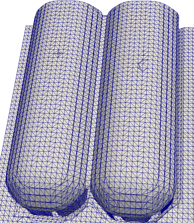
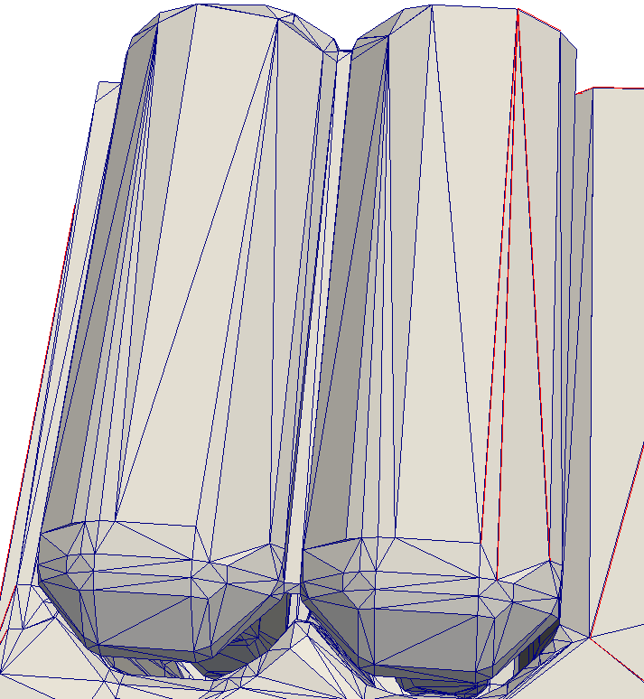
(a)	(b)

Figure 4: (a) Isosurface; (b) simplified mesh with close features in red.

Table 1: Simplification: $f$ triangles, $c_{m}$ $d$-close features, $v_{m}$ percentage vertices displaced, $a_{m}$ median and $m_{m}$ max displacement in units of $d$ for modification, likewise $c_{e},v_{e},a_{e},m_{e}$ for expansion and $v_{o},a_{o},m_{o}$ for optimization, and $t$ seconds running time.

sec.	$f$	$c_{m}$	$v_{m}$	$a_{m}$	$m_{m}$	$c_{e}$	$v_{e}$	$a_{e}$	$m_{e}$	$v_{o}$	$a_{o}$	$m_{o}$	$t$
7.1	34876	36	0.00	0.00	0.00	8	0.02	0.00	0.00	0.02	0.00	0.00	1.23
	35898	36	0.00	0.00	0.00	8	0.02	0.00	0.00	0.02	0.00	0.00	1.26
	123534	2	0.00	0.00	0.00	0	0.00	0.00	0.00	0.00	0.00	0.00	2.36
	125394	5	0.00	0.00	0.00	0	0.00	0.00	0.00	0.00	0.00	0.00	2.37
	1596	139	0.37	0.56	0.65	11	0.50	0.18	0.30	0.50	0.17	0.25	0.45
	2568	177	0.07	0.13	0.13	66	2.41	0.85	3.00	2.41	0.48	1.25	4.33
7.2	377534	5119	0.13	0.01	0.70	69	0.01	0.60	2.14	0.01	0.46	2.24	15.58
	407014	18727	0.54	0.02	0.71	149	0.02	0.36	1.71	0.02	0.32	1.45	22.45
	436308	23980	0.23	0.33	1.02	441	0.07	0.48	2.21	0.07	0.41	1.57	211.00
	438364	291	0.00	0.40	0.83	11	0.00	0.36	0.73	0.00	0.36	0.72	8.60
	641604	221	0.00	0.53	0.70	14	0.00	0.48	0.89	0.00	0.46	0.86	11.83
	667838	329	0.00	0.54	0.94	13	0.00	0.51	1.03	0.00	0.47	0.83	10.06
	773236	235	0.00	0.30	0.48	7	0.00	0.43	1.00	0.00	0.36	0.98	14.62
7.3	1572	1916	5.69	0.07	0.55	120	1.89	0.85	2.45	3.67	0.74	2.24	5.32
	1612	2614	6.91	0.08	0.74	81	1.85	0.85	2.45	3.95	0.68	1.98	3.83
7.4	465546	1363142	18.54	0.08	1.04	9250	1.44	0.85	3.01	0.00	0.00	0.00	299.90
	473542	1506798	14.39	0.08	1.31	12186	2.34	0.59	3.05	0.00	0.00	0.00	459.50
7.5	125986	4	0.00	0.00	0.00	4	0.07	0.83	1.00	0.07	0.83	2.83	14.59
	154084	0	0.00	0.00	0.00	0	0.00	0.00	0.00	0.00	0.00	0.00	3.03

7.2 Minkowski sums

The inputs are Minkowski sums of pairs of polyhedra with 53 bit vertex coordinates (Fig. 5). We construct the Minkowski sums robustly using our prior algorithm [3], but without perturbing the input. The output vertex coordinates are ratios of degree 7 and degree 6 polynomials in the input coordinates, hence have about 800 bit precision.

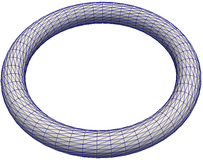
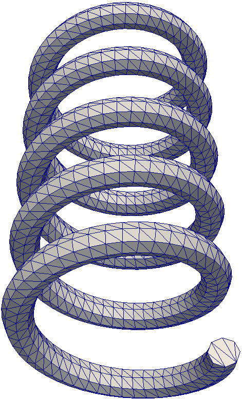
(a)	(b)
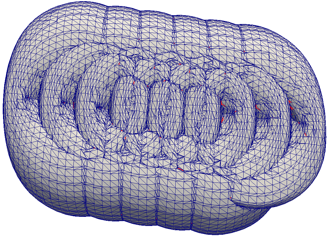
(c)

Figure 5: (a) Torus, (b) helix, (c) Minkowski sum with close features in red.

We test 10 polyhedra with up to 40,000 triangles. The 55 pairs have Minkowski sums with median 32,000 and maximum 773,000 triangles, and median 80 and maximum 37,000 close features. Modification reduces the number of close features to median 0 and maximum 440, and displaces median 0.01% and maximum 0.58% of the vertices with median and maximum displacements of $0.15d$ and $d$. Expansion displaces median 0.0% and maximum 0.07% of the vertices with median and maximum displacements of $0.0d$ and $5.33d$. Optimization does not help. The median and maximum running times per input triangle are $2\times 10^{-5}$ and $0.001$ seconds. Table 1 shows the results for the seven largest inputs.

7.3 Sweeps

The inputs are approximate 4D free spaces for a polyhedral robot that rotates around the $z$ axis and translates freely relative to a polyhedral obstacle. The algorithm is as follows. We split the rotation into short intervals. Within an interval, we approximate the free space by the Minkowski sum of the obstacle with the complement of the volume swept by the robot as it rotates around the axis. We employ a rational parameterization of the rotation matrix with parameter $t$. The coordinates of a rotated vertex are ratios of polynomials that are quadratic in $t$ and linear in the input coordinates, for total degree 6. The highest precision vertices of the swept volume are intersection points of three triangles comprised of rotated vertices. The degree of their coordinates is $13\times 6=78$ and the input has 27 bit precision, so the output precision is about 2100 bits.

We test a robot with 12 triangles and an obstacle with 64 triangles (Fig. 6). We use 40 equal rotation angle intervals. The inputs have 1,400 to 1,600 triangles, and median 1,600 maximum 3,600 close features. Modification reduces the number of close features to median 70 maximum 140, and displaces median 5.2% and maximum 8.5% of the vertices with median and maximum displacements of $0.08d$ and $0.87d$. Expansion displaces median 2.0% and maximum 2.2% of the vertices with median and maximum displacements of $0.86d$ and $2.46d$, which optimization changes to $0.57d$ and $6.1d$. The median and maximum running times per input triangle are 0.004 and 0.02 seconds. Table 1 shows the results for the two largest inputs.

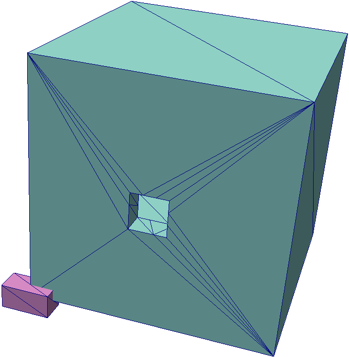
(a)

(b)

(c)

Figure 6: (a) Robot (purple) and obstacle (blue) with outer and inner cells. (b) Swept volume of robot over one angle interval (magnified). (c) Approximate free space for this interval with close features in red.

7.4 Free spaces

The inputs are triangulated 3D free spaces for a polyhedral robot that rotates around the $z$ axis and translates freely in the $xy$ plane relative to a stationary polyhedron (Fig. 7), which we compute with our prior algorithm [15]. The free space coordinates are $(x,y,t)$ with $t$ a rational parameterization of the rotation angle. The $t$ coordinates of the vertices are zeros of quartic polynomials whose coefficients are polynomials in the coordinates of the input vertices. Their algebraic degree and precision are far higher than in the previous tests.

We test four robots with 4 to 42 triangles and four obstacles with 736 to 8068 triangles. The 16 free spaces have median 125,000 and maximum 474,000 triangles, and median 530,000 and maximum 1,507,000 close features. Modification reduces the number of close features to median 2,400 max 12,000, and displaces median 17% and maximum 26% of the vertices with median and maximum displacements of $0.07d$ and $1.31d$. Expansion displaces median 1% and maximum 5% of the vertices with median and maximum displacements of $0.8d$ and $8d$. Optimization barely reduces the displacement and is slow, so we omit it from the results. The median and maximum running times per input triangle are 0.001 and 0.002 seconds. Table 1 shows the results for the two largest inputs.

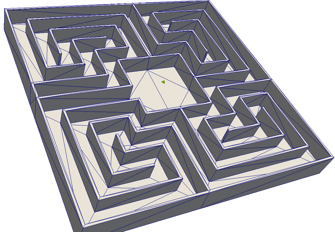
(a)

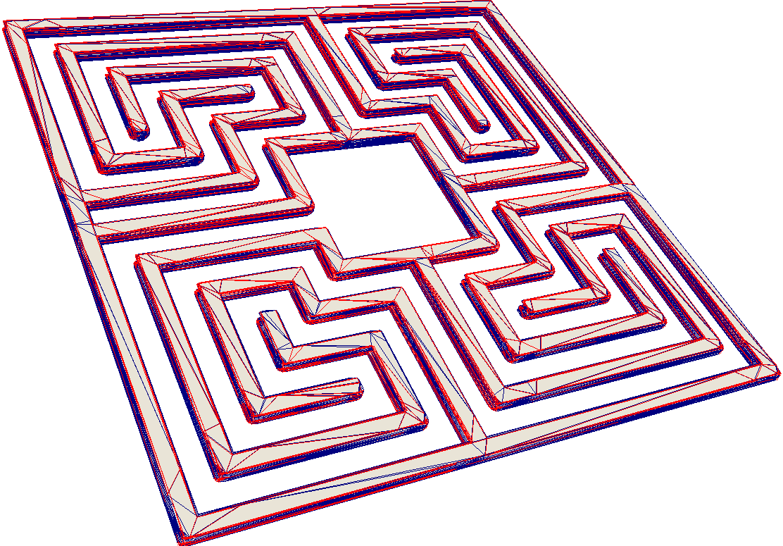
(b)

Figure 7: (a) Robot in maze; (b) configuration space with close features in red.

Figure 8: Polyhedron whose tetrahedral mesh has 150,000 triangles.

7.5 Tetrahedral meshes

The inputs are eight Delaunay tetrahedralizations with 3,000 to 150,000 triangles, and median 20 maximum 500 close features (Fig. 8). Modification does nothing because no edge is incident on two triangles. Expansion displaces median 4.9% and maximum 30% of the vertices with median and maximum displacements of $0.75d$ and $3.96d$. Optimization does not help. The median and maximum running times per mesh triangle are $9\times 10^{-5}$ and $5\times 10^{-4}$ seconds. Table 1 shows the results for the two largest inputs.

8 Conclusion

The feature separation algorithm performs well on a wide range of inputs. The isosurfaces and the tetrahedral meshes have few close features and 53 bit precision. The Minkowski sums have median 80 close features and 700 bit precision. The sweeps have median 1600 close features and 2100 bit precision. The free spaces have median 530,000 close features and even higher precision. In every case, the number of displaced vertices is proportional to the number of close features, the median vertex displacement is bounded by $d$, and the running time is proportional to the number of triangles plus close features with a mild dependency on the input precision.

This performance corresponds to the assumption that every pair of close features is far from every other pair. The complexity of modification is linear in the number of short edges and skinny triangles because mesh edits do not create close features. The error is bounded by $d$ because a vertex is displaced at most once. The expansion LP achieves the optimal displacement with $\Delta=d$ because the truncation error is negligible. Thus, the number of steps is constant. Optimization converges in a few steps because the initial displacement is close to $d$. A more realistic assumption is that every pair of close features is close to a bounded number of close features. A complexity analysis under this assumption is a topic for future work.

We tested the benefit of modification by performing feature separation via expansion alone. The median vertex displacement increases slightly, the mesh size increases proportionally to the number of short edges, and the running time increases sharply. To understand the small change in displacement, consider two vertices that are $e$ apart. Modification displaces them by $e/2$, versus $(d-e)/2$ for expansion. Assuming that $e$ is uniform on $[0,d]$, the average displacement is the same. The running time increases because mesh edits take constant time, whereas expansion is quadratic in the number of close features.

We compared our linear distance function, which picks the $l$ and $m$ values, to the standard function in which $l$ and $m$ are constants. If $l$ and $m$ are not bounded, the two formulations are equivalent. (We omit the lengthy proof.) The unbounded version is much slower that our version. If $l$ and $m$ are bounded by 1 instead of 0.001, little changes. If they are set to zero, the running time drops, the error grows, and in rare cases expansion does not converge.

We conclude that modification plus expansion achieve feature separation quickly and with a small displacement. Optimization rarely achieves even a factor of two reduction in displacement and sometimes is expensive. Perhaps the reduction could be increased by global optimization of the displacement subject to the separation constraints, but this seems impractical because the constraints have high dimension, are piecewise polynomial, and are not convex.

The results on tetrahedral meshes suggest that feature separation can play a role in mesh improvement. It simultaneously improves the close features by displacing multiple vertices in a locally optimal manner, whereas prior work optimizes one vertex at a time. The tests show that the simultaneous approach is fast and effective. It readily extends to control other aspects of the mesh, such as triangle normals. Applying the approach to other mesh improvement tasks is a topic for future work.

Vitae

Sacks is a professor in the Department of Computer Science of Purdue University. His research interests are Computational Geometry, Computer Graphics, and Mechanical Design. Butt is a lead principal engineer at Autodesk. He received his PhD from Purdue in 2017 under the supervision of Sacks. Milenkovic is a professor in the Department of Computer Science of the University of Miami. His interests are Computational Geometry, Packing and Nesting, Graphics, and Visualization.

References

- [1] Exact computational geometry, http://cs.nyu.edu/exact.
- [2] E. Sacks, V. Milenkovic, Robust cascading of operations on polyhedra, Computer-Aided Design 46 (2014) 216–220.
- [3] M.-H. Kyung, E. Sacks, V. Milenkovic, Robust polyhedral Minkowski sums with GPU implementation, Computer-Aided Design 67–68 (2015) 48–57.
- [4] Cgal, Computational Geometry Algorithms Library, http://www.cgal.org.
- [5] D. Halperin, E. Packer, Iterated snap rounding, Computational Geometry: Theory and Applications 23 (2) (2002) 209–222.
- [6] V. Milenkovic, Shortest path geometric rounding, Algorithmica 27 (1) (2000) 57–86.
- [7] M. T. Goodrich, L. J. Guibas, J. Hershberger, P. J. Tanenbaum, Snap rounding line segments efficiently in two and three dimensions, in: Symposium on Computational Geometry, 1997, pp. 284–293.
- [8] S. Fortune, Vertex-rounding a three-dimensional polyhedral subdivision, Discrete and Computational Geometry 22 (1999) 593–618.
- [9] S. Fortune, Polyhedral modelling with multiprecision integer arithmetic, Computer-Aided Design 29 (2) (1997) 123–133.
- [10] Q. Zhou, E. Grinspun, D. Zorin, A. Jacobson, Mesh arrangements for solid geometry, ACM Transactions on Graphics 35 (4) (2016) 39:1–39:15.
- [11] P. Cignoni, C. Montani, R. Scopigno, A comparison of mesh simplification algorithms, Computers and Graphics 22 (1) (1998) 37–54.
- [12] L. A. Freitag, P. Plassmann, Local optimization-based simplicial mesh untangling and improvement, International Journal of Numerical Methods in Engineering 49 (2000) 109–125.
- [13] P. M. Knupp, Hexahedral and tetrahedral mesh untangling, Engineering with Computers 17 (3) (2001) 261–268.
- [14] S.-W. Cheng, T. K. Dey, J. Shewchuk, Delaunay Mesh Generation, Chapman and Hall, 2012.
- [15] E. Sacks, N. Butt, V. Milenkovic, Robust free space construction for a polyhedron with planar motion, Computer-Aided Design 90C (2017) 18–26.
Vitae