Rapidity gap distribution in diffractive deep-inelastic scattering and parton genealogy

Abstract

We propose a partonic picture for high-mass diffractive dissociation events in onium-nucleus scattering, which leads to simple and robust predictions for the distribution of the sizes of gaps in diffractive dissociation of virtual photons off nuclei at very high energies. We show that the obtained probability distribution can formally be identified to the distribution of the decay time of the most recent common ancestor of a set of objects generated near the edge of a branching random walk, and explain the physical origin of this appealing correspondence. We then use the fact that the diffractive cross section conditioned to a minimum rapidity gap size obeys a set of Balitsky-Kovchegov equations in order to test numerically our analytical predictions. Furthermore, we show how simulations in the framework of a Monte Carlo implementation of the QCD evolution support our picture.

1 Introduction

In scattering processes at energies much larger than the typical mass of the hadrons (for a review on high-energy scattering, see Ref. [1]), a nucleus appears as a weakly bound system of nucleons, themselves made of dense sets of partons. Therefore, a classical intuition may lead one to think that in such processes, the nucleus would be ripped apart and decay into many hadrons with probability one.

Instead, it turns out that the scattering of a hadronic projectile or of a virtual photon off a target (which may be a nucleus or a proton) leaves the latter intact with a significant probability, which even tends to $\frac{1}{2}$ at asymptotically high energies. This phenomenon is predicted by basic quantum mechanics: It is just ordinary diffraction. Experimentally, it was clearly observed in proton and antiproton collisions (for reviews, see [2, 3]), also in proton-nucleus collisions (the nucleus being left intact, which is the case we are interested in here) at CERN [4], and later in virtual photon-proton scattering at DESY HERA [5, 6] (for a review, see Ref. [7]).

A priori, diffractive dissociation of a virtual photon is not very naturally formulated in a traditional perturbative QCD framework, at variance with the total deep-inelastic scattering cross sections for example. A continuous effort has been made in trying to set up a partonic interpretation of diffraction. It was recognized early that describing diffraction as bare color dipole Fock states of the virtual photon exchanging a set of globally color-neutral gluons with the target was a fine theoretical picture as a starting point [8], which can explain qualitatively the relatively large fraction of diffractive events (about 10%) observed in the HERA data [9]. Different authors have refined this picture by incorporating small-$x$ QCD evolution or/and shadowing corrections (see e.g. [10, 11, 12]), others instead have developed a QCD factorization scheme for diffractive processes, introducing diffractive parton densities (see e.g. [13]).

A major phenomenological success of saturation models such as the Golec-Biernat and Wüsthoff model is that they have been able to describe both diffractive and inclusive cross sections in the very same formalism [14]. This success fostered many other developments, phenomenological (see e.g. Ref. [15]) as well as theoretical. Among the latter, of particular interest for us are the works aimed at establishing and studying nonlinear evolution equations for high-mass diffractive cross sections [16, 17, 18, 19, 20, 21, 22].

In the present paper, we derive robust new theoretical predictions for the distribution of rapidity gaps in the diffractive dissociation of a small-size onium (which in an experiment may be sourced by virtual photons picked from the field of a lepton) off a large nucleus. We show that this distribution is the same – up to the overall normalization – as the distribution of the age of the most recent common ancestor of extreme particles in branching random walks. We also rederive evolution equations for high-mass diffractive cross sections: We recover the fact that they may be obtained as the solution of Balitsky-Kovchegov equations. A numerical implementation of the latter enables us to check our analytical calculation of the distribution of the size of the rapidity gap.

Our paper is organized as follows. In Sec. 2, after a short review of high-energy evolution and scattering, we introduce our picture of diffraction, and explain how it connects to the general problem of ancestry in branching random walks. In Sec. 3, we show how to formulate rigorously diffractive cross sections as solutions to a system of Balitsky-Kovchegov equations, which enables accurate numerical checks of our expression for the distribution of gaps. Our numerical results are presented in Sec. 4.

2 Gap distribution and statistics of common ancestors

2.1 Short review on high-energy evolution and scattering

In this section and throughout this paper, we will consider an onium of transverse size $x_{01}$ interacting with a large nucleus.

2.1.1 Diagonal $S$-matrix elements and their evolution

Most generally, the interaction cross section can be decomposed in its elastic and inelastic components $\sigma_{\text{el}}$ and $\sigma_{\text{in}}$, the total cross section $\sigma_{\text{tot}}$ being the sum of the latter two. (By “cross section” we always mean the dimensionless quantity “cross section per unit surface in transverse space” parametrized by the impact parameter $b$, which for simplicity, we denote by $\sigma$ instead of $d\sigma/d^{2}b$.) These cross sections may be expressed with the help of the $S$-matrix element $S(x_{01})$ for the elastic scattering of the dipole off the nucleus:

$${\sigma_{\text{el}}}(x_{01})=\left|1-S(x_{01})\right|^{2}\ ,\quad{\sigma_{\text{in}}}(x_{01})=1-\left|S(x_{01})\right|^{2}\ ,\quad{\sigma_{\text{tot}}}(x_{01})=2\left[1-\text{Re}\,S(x_{01})\right].$$ (1)

At very high energies, $S$ is essentially real and ranges between $0$ and $1$, so the modulus and real part can be dropped in the above formulae. It is also useful to introduce the scattering amplitude $T(x_{01})=1-S(x_{01})$.

These formulae are general, not dependent on the microscopic theory. In QCD, an equation for the change in $S$ as the center-of-mass energy (or, equivalently, the total rapidity $y$) is increased can be written down. It is the Balitsky-Kovchegov (BK) equation [23, 24], established in the framework of the color dipole model [25] and which reads

$$\frac{\partial S(x_{01},y)}{\partial y}=\bar{\alpha}\int\frac{d^{2}x_{2}}{2\pi}\frac{x_{01}^{2}}{x_{02}^{2}x_{12}^{2}}\left[S(x_{02},y)S(x_{12},y)-S(x_{01},y)\right],$$ (2)

where we made the $y$-dependence explicit, and we introduced the usual notation $\bar{\alpha}=\alpha_{s}N_{c}/\pi$. The initial condition is a function of $x_{01}$ representing the $S$-matrix element at some starting rapidity, say $y=0$. For the latter, one can use the McLerran-Venugopalan (MV) model [26], representing the interaction of a dipole of size $x_{01}$ with the nucleus characterized by the momentum scale $Q_{\text{MV}}$:

$$S_{\text{MV}}(x_{01})=\exp\left[-\frac{x_{01}^{2}Q_{\text{MV}}^{2}}{4}\ln\left(e+\frac{4}{x_{01}^{2}\Lambda^{2}}\right)\right].$$ (3)

$\Lambda$ is the QCD scale. We see that $S_{\text{MV}}$ is then a function smoothly and monotonously connecting $S_{\text{MV}}=1$ for $x_{01}\rightarrow 0$ to $S_{\text{MV}}=0$ for $x_{01}\rightarrow+\infty$, with a sharp transition occurring around the size $2/Q_{\text{MV}}$.

The solution to the BK equation is not known, but some of its essential properties have been derived, see Ref. [27, 28, 29]. In particular, asymptotically for large $y$, it converges to a traveling wave, which at fixed $y$ is again a smooth function of $x_{01}$ connecting 1 and 0, whose evolution with $y$ amounts to a mere translation in $x_{01}$. The transition between $S=1$ and $S=0$ occurs at some $y$-dependent size $2/Q_{s}(y)$, where $Q_{s}(y)$ is the saturation momentum, defined for example by requiring that

$$S(x_{01}=2/Q_{s}(y),y)=\frac{1}{2}.$$ (4)

With an initial condition such as the MV model, the analytic expression of the amplitude $T=1-S$ around the transition region reads

$$T(x_{01},y)=c_{T}\ln\frac{1}{x_{01}^{2}Q_{s}^{2}(y)}\left[x_{01}^{2}Q_{s}^{2}(y)\right]^{\gamma_{0}}\exp\left\{-\frac{\ln^{2}[x_{01}^{2}Q_{s}^{2}(y)]}{2\bar{\alpha}y\chi^{\prime\prime}(\gamma_{0})}\right\}.$$ (5)

(A precise definition of the validity domain will be given in Eq. (9) below). $c_{T}$ is a constant and the saturation momentum reads, for large $y$,

$$Q_{s}^{2}(y)=Q_{\text{MV}}^{2}\frac{e^{\bar{\alpha}y\chi^{\prime}(\gamma_{0})}}{({\bar{\alpha}y})^{3/(2\gamma_{0})}},$$ (6)

up to an overall constant of order one not explicitely written here, which depends on the very definition of the saturation scale. The function

$$\chi(\gamma)=2\psi(1)-\psi(\gamma)-\psi(1-\gamma)$$ (7)

is up to a factor $\bar{\alpha}$ the usual eigenvalue of the BFKL kernel corresponding to the eigenfunction $x_{01}^{2\gamma}$. $\gamma_{0}$ is defined to be the solution to the equation $\chi(\gamma_{0})/\gamma_{0}=\chi^{\prime}(\gamma_{0})$. In numbers,

$$\gamma_{0}=0.627549\cdots,\quad\chi(\gamma_{0})=3.0645\cdots,\quad\chi^{\prime\prime}(\gamma_{0})=48.5176\cdots$$ (8)

The forms of $T$ and of the saturation momentum do not depend on the details of the initial condition, up, of course, to overall constants and subasymptotic terms in the rapidity. The expression (5) is valid in the so-called (geometric) scaling region [30] but nevertheless for $x_{01}\ll 1/Q_{s}(y)$. The scaling region is defined as the range in $x_{01}$ in which $T$, which is a priori a function of the two variables $x_{01}$ and $y$, becomes effectively a function of the single composite variable $x_{01}Q_{s}(y)$ only. Hence parametrically, $x_{01}$ needs to obey the following inequalities:

$$1<|\ln[x_{01}^{2}Q_{s}^{2}(y)]|\leq\sqrt{\bar{\alpha}y\chi^{\prime\prime}(\gamma_{0})}.$$ (9)

In this region, the scattering is weak ($T\ll 1$) but the value of the amplitude is influenced by the presence of a saturated nucleus, which, technically, acts as an absorptive boundary.

2.1.2 Interpretation of the BK equation

Let us interpret physically the BK equation.

Assume that the total rapidity available for the scattering is $Y$. Integrating Eq. (2) up to $y=Y$, we get $T(x_{01},Y)$ which we may view as the elastic scattering amplitude for the interaction of an elementary dipole of size $x_{01}$ off a nucleus evolved to rapidity $Y$. This is the dipole restframe picture. In this frame, the nucleus looks the same in each event: It is a dense set of gluons, whose density grows deterministically with the rapidity. The density of the gluons in the nucleus determines the probability amplitude for the onium to interact with it.

One can have a completely different interpretation by going for example to the restframe of the nucleus. (See Ref. [31] where these ideas were developed). In that frame, the onium carries the full rapidity $Y$ and thus is in a highly-evolved quantum state at the time of its interaction with the nucleus. This quantum state is conveniently represented by a set of dipoles, differing from an event to another one, constructed stochastically through a $1\rightarrow 2$ branching diffusion process whose characteristics are encoded in the kernel of the BK equation. Indeed, the probability that a dipole of size $x_{01}$ splits by emission of a gluon at transverse position $x_{2}$ up to $d^{2}x_{2}$ into two dipoles of sizes $x_{02}$ and $x_{12}$ when one increases its rapidity by the infinitesimal quantity $d\tilde{y}$ reads [25]

$$\text{proba}(x_{01}\rightarrow x_{02},x_{12})=\bar{\alpha}\,d\tilde{y}\,\frac{d^{2}x_{2}}{2\pi}\frac{x_{01}^{2}}{x_{02}^{2}x_{12}^{2}}.$$ (10)

The scattering amplitude $T(x_{01},Y)$ is then related to the probability $P(x_{01},Y|1/Q_{\text{MV}})$ to find at least one dipole in the onium Fock state at rapidity $\tilde{y}=Y$ whose size is larger than $R=1/Q_{\text{MV}}$. The BK equation then appears as an equation for the statistics of the size of the largest dipole in a branching diffusion process.

More precisely, $P$ solves the BK equation written in the form

$$\frac{\partial P(x_{01},\tilde{y}|R)}{\partial\tilde{y}}=\bar{\alpha}\int\frac{d^{2}x_{2}}{2\pi}\frac{x_{01}^{2}}{x_{02}^{2}x_{12}^{2}}[P(x_{02},\tilde{y}|R)+P(x_{12},\tilde{y}|R)-P(x_{01},\tilde{y}|R)\\ -P(x_{02},\tilde{y}|R)P(x_{12},\tilde{y}|R)].$$ (11)

This equation is the same equation as the one solved by $T=1-S$. The initial conditions however differ: The one for $T$ is e.g. the MV model, while the one for $P$ is a mere Heaviside distribution

$$P(x_{01},\tilde{y}=0|R)=\theta\left(\ln\frac{x_{01}^{2}}{R^{2}}\right)$$ (12)

when the initial state of the onium consists in a single dipole of size $x_{01}$. Although the initial conditions are different, the asymptotic large-rapidity solutions fall into the very same universality class. It is this mathematical property which enables the identification of the asymptotics of the scattering amplitude of a dipole of size $x_{01}$ off a nucleus characterized by the saturation momentum $Q_{\text{MV}}$ at total rapidity $Y$ with the probability of finding (at least) a dipole of size larger than $1/Q_{\text{MV}}$ at rapidity $Y$ in an initial onium of size $x_{01}$:

$$T(x_{01},Y)\underset{\text{large $Y$}}{\simeq}P(x_{01},Y|1/Q_{\text{MV}}).$$ (13)

For completeness and because we will use it below, let us write explicitely the expression of $P$, which is tantamount to the expression of $T$ up to the appropriate substitutions:

$$P(x_{01},\tilde{y}|R)=c_{P}\ln\frac{R^{2}}{x_{\perp}^{2}(\tilde{y})}\left[\frac{x_{\perp}^{2}(\tilde{y})}{R^{2}}\right]^{\gamma_{0}}\exp\left\{-\frac{\ln^{2}[R^{2}/x_{\perp}^{2}(\tilde{y})]}{2\bar{\alpha}\tilde{y}\chi^{\prime\prime}(\gamma_{0})}\right\}$$ (14)

(compare to Eq. (5)). $c_{P}$ is a constant and

$$x_{\perp}^{2}(\tilde{y})=x_{01}^{2}\frac{e^{\bar{\alpha}\tilde{y}\chi^{\prime}(\gamma_{0})}}{(\bar{\alpha}\tilde{y})^{3/(2\gamma_{0})}},$$ (15)

up to a constant which again is a matter of definition.

The interpretation of $x_{\perp}(\tilde{y})$ is the following. It is the size for which the probability to have a dipole of that size in the Fock state of the onium at rapidity $\tilde{y}$ is some predefined number, say 1. If one draws the histogram of the dipole sizes at rapidity $\tilde{y}$ in a particular event, $x_{\perp}$ is the expected position of its tip (towards large sizes). Consequently, dipoles of sizes much larger than $x_{\perp}$ can only stem from rare fluctuations in the stochastic evolution.

The probability of having such fluctuations in a realization of the onium evolution is precisely given by Eq. (14). In the same way as for $T$, there is a region defined by Eq. (9) (with the substitutions $y\rightarrow\tilde{y}$, $Q_{s}(y)\rightarrow 1/x_{\perp}(\tilde{y})$) in which the probability to find a fluctuation obeys a scaling law, and out of which (for very large $R$) $P$ is strongly suppressed by the Gaussian factor in the log of the sizes appearing in Eq. (14).

2.2 Rapidity gaps and large fluctuations

We are now in a position to introduce our picture of diffraction. We shall start by defining diffractive versus elastic events, before moving on to the microscopic description of diffractive events and eventually to the quantitative predictions which directly follow.

2.2.1 Elastic and diffractive events

Elastic events are, at least theoretically, straightforward to define: The particles in the final state are the same as the ones in the initial state; Only their momenta are redistributed. In order to observe a significant fraction of elastic events, one needs that the $S$-matrix be close to 0. Indeed, in this case, according to Eq. (1)

$$\sigma_{\text{el}}\simeq\sigma_{\text{in}}\simeq\sigma_{\text{tot}}/2,$$ (16)

and the ratio $\sigma_{\text{el}}/\sigma_{\text{tot}}$ is maximum. These equalities are characteristic of the scattering of quantum particles off a black disk: The inelastic cross section corresponds to the absorption by the disk, while the elastic cross section is due to the particles which are diffracted in its shadow.

For a single elementary dipole (i.e. an onium in its ground state) that scatters off a nucleus, $S=0$ is verified whenever the size of the dipole is much larger than the inverse saturation momentum $1/Q_{s}(Y)$ of the nucleus ($Y$ is the rapidity of the nucleus in the frame of the dipole, namely the total available rapidity). In this case, elastic scattering is observed in half of the events.

If instead the size of the onium is very small compared to the inverse saturation momentum, then $S\sim 1$, and the total cross section is dominated by the inelastic events:

$$\sigma_{\text{in}}=(1+S)(1-S)\simeq 2(1-S)=\sigma_{\text{tot}}\gg(1-S)^{2}=\sigma_{\text{el}}$$ (17)

Hence one may think that a small onium (small compared to $1/Q_{s}(Y)$) would almost exclusively trigger inelastic events since its inelastic cross section is small, but its elastic cross section is even much smaller. This is however not true, because in a high-energy scattering, the onium does not interact as a bare dipole state but through complicated quantum fluctuations, and the latter may interact elastically with a significant probability. Such realizations of the onium state do not result in elastic events, but in diffractive ones, which we shall now define more precisely.

To define diffractive events, we do not require that both interacting particles remain of the same nature. We just require that the nucleus does not completely break up in the scattering. It may remain strictly intact or scatter to an excited state, which subsequently returns to an energy minimum through fission. The scattering is coherent or quasi-elastic, at the level of the nucleus. In any case, there is a region in rapidity (namely in angle in a detector) around the decay products of the nucleus in which no particle is seen. Requiring that there be a rapidity gap is a good practical definition, and was a striking signature of diffractive events at HERA. The onium instead may undergo a transition to a complicated system of many hadrons which materialize in the final state (see Fig. 1). This is what happens if we ask for a high-mass diffractive final state.

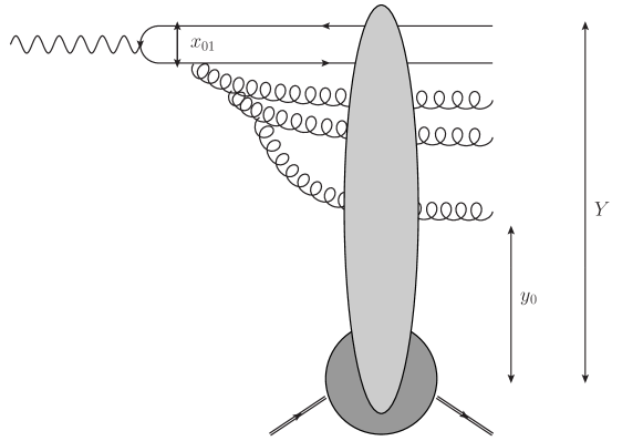
Figure 1: Graph contributing to the amplitude for high-mass diffraction in deep-inelastic scattering, with a rapidity gap $y_{0}$. The virtual photon converts to an onium of size $x_{01}$, which scatters through a Fock state made of the initial $q\bar{q}$ pair together with soft gluons. The elongated blob represents the exchange of a color singlet between the state of the onium and the nucleus resulting in an elastic scattering.

Coming back to onium-nucleus scattering and with a view at sorting out the diffractive dissociative events, it is useful to picture the scattering in a frame in which the onium is not at rest: Let us give it the rapidity $\tilde{y}_{0}\gg 1$, while the nucleus takes the remaining available rapidity $y_{0}=Y-\tilde{y}_{0}$. Then the onium does not interact as a bare $q\bar{q}$ dipole state, but as a quantum state made of many gluons (conveniently represented by a set of dipoles). In such quantum states, there may be a few unusually large dipoles, of sizes greater than $1/Q_{s}(y_{0})$. These dipoles interact with the nucleus with a probability of order 1. If furthermore their size lie deep in the saturation region, the interaction with the nucleus is elastic in half of the events. This results in a rapidity gap whose size is of the order of the remaining rapidity, namely $Y-\tilde{y}_{0}=y_{0}$. At the same time, because the different components of the Fock state interact all differently, the coherence is broken at the level of the onium and the partons present in its Fock state at rapidity $\tilde{y}_{0}$ materialize in the form of a hadronic system in the fragmentation region of the latter. This is precisely diffractive dissociation.

So the key for describing diffractive events is a proper understanding of the event-by-event fluctuations of the large-dipole component of the onium quantum state.

2.2.2 Fluctuations in onium evolution

For $x_{01}$ small enough with respect to $1/Q_{s}(Y)$, the mechanism for the production of an unusually large dipole (that crosses the saturation boundary at rapidity $\tilde{y}_{0}=Y-y_{0}$ with respect to the onium, up to typically one unit) in the Fock state of an onium was studied in detail in Ref. [31, 34]. There, we identified two types of fluctuations that may occur in the course of the rapidity evolution: The front fluctuations and the tip fluctuations.

In the beginning of the onium evolution, i.e. at low rapidities $\tilde{y}$, the state is dilute and thus subject to fluctuations which strongly determine the size of the largest dipole in the event at any later rapidity. We shall call this size “position of the tip of the front” by reference to the traveling wave language, and the kind of fluctuations which lead to this effect “front fluctuations”.

At rapidity $\tilde{y}_{0}$ (up to $\Delta\sim 1/\bar{\alpha}$), a fluctuation at the tip of the front may happen, containing one or a few dipoles typically larger by an order of magnitude with respect to the largest dipole in the absence of the fluctuation. The latter fluctuation is short-lived because it is rapidly absorbed by the bulk of the front, which moves with a velocity larger than that of the tip of the front stemming from the fluctuation. This is what we call a “tip fluctuation”, and is quite different in nature from the front fluctuations: The memory of the latter is conserved throughout the evolution, whereas the former moves stochastically the tip of the front forward only at the very rapidity at which it occurs.

The most favorable scenario for creating a few unusually large dipoles around the rapidity $\tilde{y}_{0}$ is to combine a front fluctuation occurring at low rapidities $\tilde{y}\simeq 0$ at which the onium still is a dilute state with a tip fluctuation at $\tilde{y}_{0}$.

Actually, it will be an essential ingredient of our calculation that the dipoles which are within the saturation region of the nucleus at rapidity $\tilde{y}_{0}$ come from this very combination of front and tip fluctuations. The analytical arguments supporting this scenario are quite technical: Therefore, we leave them for the Appendix.

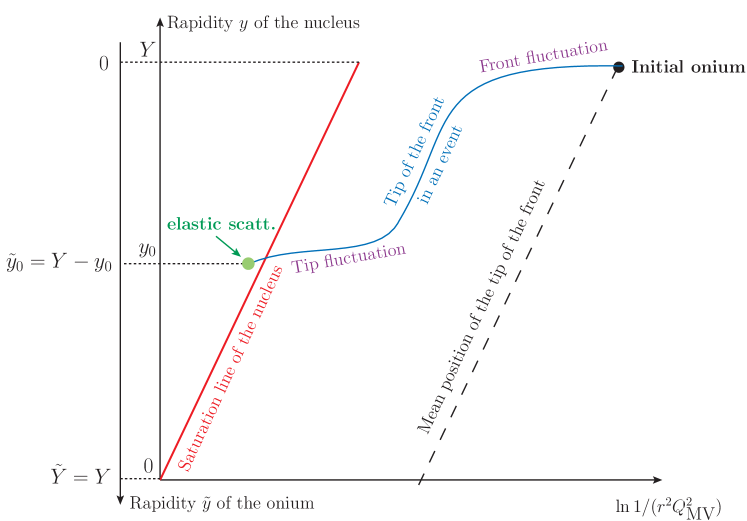
Figure 2: Schematic picture of a diffractive event with a rapidity gap of size $y_{0}$. The vertical axis oriented upwards is the rapidity of the nucleus, ranging from 0 to the total available rapidity $Y$. The rapidity of the onium is marked on the downward axis. The saturation line of the nucleus of equation $rQ_{s}(y)\sim 1$ is shown (continuous straight line), as well as the size of the largest dipole in the Fock state of the onium in this particular realization of the evolution (also called “position of the tip of the front”; continuous curly line). Its shape is determined by a front fluctuation and a tip fluctuation, which together generate a few unusually large dipoles (compared to the mean position of the tip $r=x_{\perp}(\tilde{y})$; dashed line) at rapidity $y_{0}$.

2.2.3 Quantitative evaluation of the diffractive cross section

The scenario for diffractive events is illustrated schematically in Fig. 2. Let us translate this picture into an actual quantitative evaluation of the diffractive cross section.

In our picture, a given event has a rapidity gap of size $y_{0}$ when the Fock state of the onium in this event contains at least one dipole of size larger than $1/Q_{s}(y_{0})$ at rapidity $\tilde{y}_{0}=Y-y_{0}$, namely if there is a fluctuation at that rapidity which generates a large dipole.

This means that $d\sigma_{\text{diff}}/dy_{0}$ is identical to the probability $P(x_{01},\tilde{y}_{0}|1/Q_{s}(y_{0}))$ introduced above Eq. (11),

$$\frac{d\sigma_{\text{diff}}}{dy_{0}}=P(x_{01},\tilde{y}_{0}|1/Q_{s}(y_{0})).$$ (18)

As explained before, $P$ solves the BK equation. Therefore, the following expression holds for the diffractive cross section in the scaling region and at its border (see Eq. (14)):

$$\frac{d\sigma_{\text{diff}}}{dy_{0}}=c_{\text{diff}}\left[{x_{\perp}^{2}(\tilde{y}_{0})Q_{s}^{2}(y_{0})}\right]^{\gamma_{0}}\ln\frac{1}{x_{\perp}^{2}(\tilde{y}_{0})Q_{s}^{2}(y_{0})}\exp\left\{-\frac{\ln^{2}[x_{\perp}^{2}(\tilde{y}_{0})Q_{s}^{2}(y_{0})]}{2\bar{\alpha}\tilde{y}_{0}\chi^{\prime\prime}(\gamma_{0})}\right\},$$ (19)

where $c_{\text{diff}}$ is a constant. This formula applies in the scaling region, away from the deep saturation region, which puts the following restrictions on the values of the rapidity and the size of the initial onium (see Eq. (9)):

$$1<|\ln[x_{\perp}^{2}(\tilde{y}_{0})Q_{s}^{2}(y_{0})]|\leq\sqrt{\bar{\alpha}\tilde{y}_{0}\chi^{\prime\prime}(\gamma_{0})}.$$ (20)

In order to isolate the $y_{0}$ dependence, we can rewrite Eq. (19) as

$$\boxed{\frac{d\sigma_{\text{diff}}}{dy_{0}}=c_{\text{diff}}\left[\frac{\bar{\alpha}Y}{\bar{\alpha}y_{0}\bar{\alpha}(Y-y_{0})}\right]^{3/2}\exp\left\{-\frac{\ln^{2}[x_{01}^{2}Q_{s}^{2}(Y)]}{2\bar{\alpha}(Y-y_{0})\chi^{\prime\prime}(\gamma_{0})}\right\}\times\left[x_{01}^{2}Q_{s}^{2}(Y)\right]^{\gamma_{0}}\ln\frac{1}{x_{01}^{2}Q_{s}^{2}(Y)}},$$ (21)

where we have furthermore assumed

$$\left|\ln[x_{01}^{2}Q_{s}^{2}(Y)]\right|\gg\left|\ln\frac{\bar{\alpha}Y}{\bar{\alpha}y_{0}\,\bar{\alpha}(Y-y_{0})}\right|$$ (22)

in order to be able to substitute $\ln[x_{\perp}^{2}(Y-y_{0})Q_{s}^{2}(y_{0})]$ with $\ln[x_{01}^{2}Q_{s}^{2}(Y)]$. This condition in turn requires that $y_{0}$ cannot be too close neither to $0$ nor to $Y$. Note that within this approximation, the condition (20) translates into a condition on the size of the initial onium:

$$1<|\ln[x_{01}^{2}Q_{s}^{2}(Y)]|\leq\sqrt{\bar{\alpha}Y\chi^{\prime\prime}(\gamma_{0})}.$$ (23)

These inequalities mean that we need to pick the initial dipole away from the saturation region (this is what the leftmost inequality means) but in the scaling region or at its border (rightmost inequality), in such a way that the rapidity evolution of the dipole is always driven by the eigenvalue of the BFKL kernel $\bar{\alpha}\chi(\gamma\simeq\gamma_{0})$.

Equation (21) is the main result of our paper. For fixed $Y$ and $x_{01}$, it gives the distribution of the rapidity gap in diffractive events, up to a constant which we were not able to determine analytically.

It is also interesting to compare the diffractive and total cross sections. To this aim, let us go deep into the scaling region, which allows us to neglect the Gaussian suppression factor in Eq. (21). Recalling that

$$\sigma_{\text{tot}}=c_{\text{tot}}\left[x_{01}^{2}Q_{s}^{2}(Y)\right]^{\gamma_{0}}\ln\frac{1}{x_{01}^{2}Q_{s}^{2}(Y)},$$ (24)

we arrive at

$$\boxed{\frac{1}{\sigma_{\text{tot}}}\frac{d\sigma_{\text{diff}}}{dy_{0}}=\frac{c_{\text{diff}}}{c_{\text{tot}}}\left[\frac{\bar{\alpha}Y}{\bar{\alpha}y_{0}\bar{\alpha}(Y-y_{0})}\right]^{3/2}}.$$ (25)

The $y_{0}$-dependence is completely determined by this formula. However, we do not see how we may determine the overall constant $c_{\text{diff}}/c_{\text{tot}}$ from our approach.

We are now going to explain how this is related to genealogies in branching random walks.

2.3 Parton genealogy

In this section, we draw a parallel between diffraction in hadronic physics and ancestry in general branching-diffusion processes.

Let us go to the restframe of the nucleus, in which the whole evolution is in the onium. In a given event, a few dipoles in the Fock state of the onium eventually interact with the nucleus, typically the ones that have a size larger than the inverse saturation momentum $Q_{\text{MV}}^{-1}$ of the nucleus.

We chose the initial onium in such a way that the mean position of the tip of the front was far enough from the saturation boundary of the nucleus that diffractive scattering was due to an unusually large fluctuation in the course of the evolution. It is this fluctuation which generates, through further evolution, the dipoles that eventually scatter off the nucleus in the nucleus restframe. Hence with high probability, this particular fluctuation contains the most recent common ancestor of the dipoles that interact.

A similar but not identical problem has recently been addressed by Derrida and Mottishaw in the context of the so-called Generalized Random Energy Model (GREM) [35], from which they got results that they assumed applied to branching random walks.

The kind of problem addressed there was the following. Consider e.g. a one-dimensional branching random walk. Think of branching Brownian motion for example: Independent particles diffuse on a line parametrized by the real variable $x$ in time $t$, and each of them may independently generate two offspring according to a Poisson process in time of constant intensity. Starting with one particle at $t=0$, at the final time $t=T$, each realization consists in a given finite number of particles, extending over a finite region in $x$. Let us pick the $n$ leftmost particles in each event ($n=2,3,\cdots$) and ask the following question: What is the time $t_{0}$ at which their most recent common ancestor split?

The answer was found (actually conjectured by extrapolating a calculation in the GREM) in Ref. [35]. The probability density of $t_{0}$ reads

$$p(t_{0})=\frac{1}{\gamma_{0}}\sqrt{\frac{1}{2\pi\chi^{\prime\prime}(\gamma_{0})}}\left(\frac{T}{t_{0}(T-t_{0})}\right)^{3/2}$$ (26)

Note that the overall normalization factor could also be computed in that context. $\chi(\gamma)$ is the eigenvalue function of the kernel of the equivalent of the linearized BK equation and $\gamma_{0}$ is defined to be the solution of the equation $\chi(\gamma_{0})/\gamma_{0}=\chi^{\prime}(\gamma_{0})$. Up to the replacements of the evolution variables $\bar{\alpha}Y\leftrightarrow T$, $\bar{\alpha}y_{0}\leftrightarrow t_{0}$ and up to the overall normalization, this is exactly the same answer as the one we obtained for the gap size dependence of the diffractive cross section, see Eq. (25).

We shall test this analogy numerically below in Sec. 4.2. Before, we are going to introduce the Good-Walker formulation which is very useful to set up a numerical calculation of the diffractive cross section.

3 Diffraction from the BK equation

In this section, we give a concise derivation of an equation for the diffractive cross section which was first established in Ref. [16] (see also Ref. [1], Chap. 7.2), and further studied in Ref. [17, 18]. The authors of Ref. [22] have also reestablished this equation, in a way which is very close to ours.

3.1 Good-Walker formulation of diffraction

Good and Walker gave an elegant general framework for diffractive dissociation [36], which will enable us to write exact equations for diffraction in the framework of the dipole model. Its essential ingredient is the expansion of the state of a projectile in terms of the eigenstates of the interaction of a given target off which it scatters.

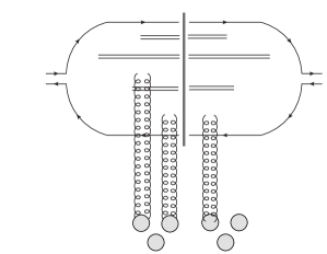
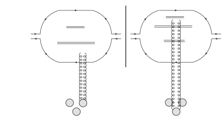
(a)	(b)

Figure 3: Picture of diagrams that lead to (a) onium diffractive dissociative and (b) elastic events. The graphs displayed contribute to $\left\langle T^{2}\right\rangle$ and to $\left\langle T\right\rangle^{2}$ respectively. In each graph, the double vertical line denotes the final state (up to hadronization), the subgraph to the left of it is the amplitude, and the one to the right the complex-conjugate amplitude.

The cross section for the diffractive dissociation of a dipole of initial size $x_{01}$ in its scattering off a nucleus at a fixed impact parameter and with a gap of minimum size $y_{0}$ reads in the Good-Walker picture

$${\sigma_{\text{diff}}}=\sum_{X}{}_{\tilde{y}_{0}}\langle x_{01}|{\mathbb{T}}^{\dagger}(y_{0})|X\rangle\langle X|{\mathbb{T}}(y_{0})|x_{01}\rangle_{\tilde{y}_{0}}-\left|{}_{\tilde{y}_{0}}\langle x_{01}|{\mathbb{T}}(y_{0})|x_{01}\rangle_{\tilde{y}_{0}}\right|^{2}\ ,$$ (27)

where $|x_{01}\rangle_{\tilde{y}_{0}}$ is the state of the initial onium evolved to the rapidity $\tilde{y}_{0}$ and ${\mathbb{T}}(y_{0})$ is the interaction matrix of the onium Fock states with a nucleus boosted to the rapidity $y_{0}$. $X$ is any dipole final state, and the sum over $X$ also contains an integration over phase space of the type $\int\prod d^{2}x_{a}dz_{a}$, where $x_{a}$ and $z_{a}$ are respectively the transverse position and the longitudinal momentum fraction of the gluons (i.e. endpoints of the dipoles). We refer the reader to [37] for an earlier application of this formula to diffractive deep-inelastic scattering, limited however to a two-dipole, i.e. $q\bar{q}g$, diffractive system. The discussion in the more recent paper of Hatta et al. addresses diffractive systems composed of any number of gluons [22], and is very close to our present discussion.

The important point to notice is that in a high-energy scattering, ${\mathbb{T}}(y_{0})$ is diagonal in coordinate space. In other words, dipoles are eigenstates of the interaction. Hence, introducing a complete set of dipoles, using the latter property and writing the wavefunction of the onium at rapidity $\tilde{y}_{0}$ on the state $|X\rangle$ as $\psi_{X}(x_{01},\tilde{y}_{0})\equiv\langle X|x_{01}\rangle_{\tilde{y}_{0}}$, Eq. (27) becomes

$${\sigma_{\text{diff}}}=\sum_{X}|\psi_{X}(x_{01},\tilde{y}_{0})|^{2}|\langle X|{\mathbb{T}}(y_{0})|X\rangle|^{2}-\left|\sum_{X}|\psi_{X}(x_{01},\tilde{y}_{0})|^{2}\langle X|{\mathbb{T}}(y_{0})|X\rangle\right|^{2}.$$ (28)

We denote by $T(\{r_{k}\},y_{0})\equiv\langle X|{\mathbb{T}}(y_{0})|X\rangle$ the (diagonal) matrix element of ${\mathbb{T}}(y_{0})$ for a state $|X\rangle$ corresponding to the set $\{r_{k}\}$ of dipoles (the $r_{k}$’s are their sizes, which are enough to characterize them completely for our purpose). It is also useful to introduce a notation for the averaging over the realizations of the Fock state of the onium at rapidity $\tilde{y}$. For a general function $f(X)$ of the dipole state $|X\rangle$, we write

$$\sum_{X}|\psi_{X}(x_{01},\tilde{y})|^{2}f(X)=\langle f(X)\rangle_{x_{01},\tilde{y}}.$$ (29)

With these notations, the diffractive cross section reads

$$\sigma_{\text{diff}}=\left\langle T^{2}(\{r_{k}\},y_{0})\right\rangle_{x_{01},Y-y_{0}}-\left\langle T(\{r_{k}\},y_{0})\right\rangle_{x_{01},Y-y_{0}}^{2}.$$ (30)

We further note that

$$T(\{r_{k}\},y_{0})=1-\prod_{k}S(r_{k},y_{0}),$$ (31)

where $S(r,y)$ is the solution of BK equation (2) for the $S$-matrix element corresponding to the forward elastic scattering of a dipole of size $r$ at rapidity $y$.

Finally, Eq. (30) can trivially be rewritten with the help of $S$ solution of the BK equation as

$$\sigma_{\text{diff}}=\left\langle\prod_{k}\left[S(r_{k},y_{0})\right]^{2}\right\rangle_{x_{01},Y-y_{0}}-\left\langle\prod_{k}S(r_{k},y_{0})\right\rangle_{x_{01},Y-y_{0}}^{2}.$$ (32)

It is useful to note that the second terms in Eqs. (30) and (32), namely $\langle T(\{r_{k}\},y_{0})\rangle^{2}$ and $\left\langle\prod_{k}S(r_{k},y_{0})\right\rangle^{2}$, are actually independant of $y_{0}$: This is a simple consequence of relativistic invariance. Since we are interested in the distribution of $y_{0}$, hence in the derivative of $\sigma_{\text{diff}}$ with respect to $y_{0}$, all $y_{0}$-independent terms can be dropped.

One could implement this formula in a computer code literally: $S(r,y)$ can be computed as a function of $r$ for different values of the rapidity $y$ by integrating the BK equation using standard methods, while the Fock states of the onium (over which one needs to average) can be generated using a Monte Carlo implementation of the dipole model, such as the one developed in Refs. [41, 42]. However, there is a way to write fully deterministic equations, which are relatively easier to integrate numerically.

3.2 Fully deterministic formulation

We are now in a position to write the diffractive cross section conditioned to the gap $y_{0}$ as a system of BK equations.

Starting from the previous discussion and introducing the notation

$$S_{2}(x_{01},\tilde{y})=\left\langle\prod_{k}[S(r_{k},y_{0})]^{2}\right\rangle_{x_{01},\tilde{y}},$$ (33)

we write

$$\frac{d\sigma_{\text{diff}}}{dy_{0}}=-\frac{\partial}{\partial y_{0}}S_{2}(x_{01},Y-y_{0}).$$ (34)

The crucial observation is that $S_{2}$ solves the BK equation. The proof that an expression like the r.h.s. of Eq. (33) obeys the BK equation is very classical in the context of branching diffusion processes (see e.g. [38]) but is less known in the context of particle physics (see however [39] and references therein). One considers a rapidity interval $\tilde{y}+d\tilde{y}$ which one decomposes in an infinitesimal interval $d\tilde{y}$, over which the initial onium may either (i) split to two dipoles with the probability (10), or (ii) remain one dipole, with the complementary probability. The evolution over the remaining rapidity interval $\tilde{y}$ produces either two independent sets of dipoles $\{r_{k_{1}}^{(1)}\}$ and $\{r_{k_{2}}^{(2)}\}$ (case (i)) or one single set $\{r_{k}\}$ (case (ii)). In equations:

$$S_{2}(x_{01},\tilde{y}+d\tilde{y})=\bar{\alpha}\,d\tilde{y}\int\frac{d^{2}x_{2}}{2\pi}\frac{x_{01}^{2}}{x_{02}^{2}x_{12}^{2}}\left\langle\prod_{k_{1}}[S(r_{k_{1}}^{(1)},y_{0})]^{2}\right\rangle_{x_{02},\tilde{y}}\left\langle\prod_{k_{2}}[S(r_{k_{2}}^{(2)},y_{0})]^{2}\right\rangle_{x_{12},\tilde{y}}\\ +\left(1-\bar{\alpha}\,d\tilde{y}\int\frac{d^{2}x_{2}}{2\pi}\frac{x_{01}^{2}}{x_{02}^{2}x_{12}^{2}}\right)\left\langle\prod_{k}[S(r_{k},y_{0})]^{2}\right\rangle_{x_{01},\tilde{y}}.$$ (35)

Taking the limit $d\tilde{y}\rightarrow 0$ and performing the appropriate replacements, we arrive indeed at the BK equation:

$$\frac{\partial}{\partial\tilde{y}}S_{2}(x_{01},\tilde{y})=\bar{\alpha}\int\frac{d^{2}x_{2}}{2\pi}\frac{x_{01}^{2}}{x_{02}^{2}x_{12}^{2}}\left[S_{2}(x_{02},\tilde{y})S_{2}(x_{12},\tilde{y})-S_{2}(x_{01},\tilde{y})\right].$$ (36)

The initial condition for $S_{2}$ reads

$$S_{2}(x_{01},\tilde{y}=0)=[S(x_{01},y_{0})]^{2},$$ (37)

where $S$ also solves the BK equation (2), with as an initial condition the $S$-matrix element for the elastic scattering of a dipole off a large nucleus at zero rapidity (3). We recognize the equations first established in Ref. [16] (for a formulation closer to ours, see Ref. [1], Sec. 7.2.2, and Ref. [22], Sec. 2). Our present work may thus also be understood as a solution to these equations endowed with an appealing interpretation.

Formulating the diffractive cross section in this way does a priori not help to address the analytical problem. But this set of BK equations (for $S$ and for $S_{2}$) is straightforward to implement and to solve numerically. Our most accurate calculation of the distribution of the rapidity gap is based on this method.

4 Numerical calculations

4.1 Diffraction as the solution of a deterministic equation

We can obtain $d\sigma_{\text{diff}}/dy_{0}$ for a given $y_{0}$ from the Good-Walker formula, integrating numerically the BK equations that follow. Such calculations were done in Ref. [17, 18, 19], but with a quite different scope.

We use a code that solves the BK equation at fixed impact parameter and in momentum space which is very similar to BKSolver developed in Ref. [40]. We shall explain very concretely how we operated it to compute $d\sigma_{\text{diff}}/dy_{0}$.

We start with a McLerran-Venugopalan initial condition for the elastic amplitude,

$$T_{\text{MV}}(r)=1-S_{\text{MV}}(r),$$ (38)

where $S_{\text{MV}}$ was given in Eq. (3), and convert it to momentum space. Generically, the transformation that realizes the mapping reads

$$\tilde{T}(k,y)=\int\frac{d^{2}r}{2\pi r^{2}}e^{ik\cdot r}T(r,y).$$ (39)

We then evolve $\tilde{T}_{\text{MV}}$ numerically to the rapidity $y_{0}$. Then, we Fourier transform $\tilde{T}(k,y_{0})$ back to coordinate space, compute the quantity $2T(r,y_{0})-T^{2}(r,y_{0})$ and evolve its Fourier transform for $\tilde{y}_{0}=Y-y_{0}$ more units of rapidity. We repeat this procedure for different values of $y_{0}$ ranging between $0$ and $Y$. The result is then expressed in coordinate space, and its $y_{0}$-derivative (up to a sign) is plotted as a function of $y_{0}$ for selected values of the initial dipole size $x_{01}$.

We consider two different values of the total rapidity: A phenomenologically realistic one, $\bar{\alpha}Y=3$, and a larger value, $\bar{\alpha}Y=20$, which enables us to better approach the asymptotics in order to test more quantitatively our picture, which should be formally exact at asymptotic rapidities. We chose to set $\Lambda=200\ \text{MeV}$ and $Q_{\text{MV}}=1\ \text{GeV}$. In what follows, the momenta and distances will always be expressed in units of $Q_{\text{MV}}$ and of $Q^{-1}_{\text{MV}}$ respectively.

We evolve the scattering amplitude of a dipole of size $x_{01}$ with the nucleus through the BK equation. We first measure the saturation scale $Q_{s}(Y)$ at rapidity $Y$ defining it as $S(x_{01}=2/Q_{s}(Y),Y)=\frac{1}{2}$. For $\bar{\alpha}Y=3$, we find $Q_{s}(\bar{\alpha}Y=3)\simeq 230$ and for $\bar{\alpha}Y=20$, $Q_{s}(\bar{\alpha}Y=20)\simeq 2\times 10^{19}$, consistently in order of magnitude with the asymptotic formula $Q_{s}^{2}(Y)\simeq Q_{\text{MV}}^{2}e^{\bar{\alpha}Y\chi^{\prime}(\gamma_{0})}/(\bar{\alpha}Y)^{3/2}$ which gives $Q_{s}(\bar{\alpha}Y=3)\simeq 665$ and $Q_{s}(\bar{\alpha}Y=20)\simeq 1.7\times 10^{20}$ respectively.

Then, we compute $\sigma_{\text{diff}}$ for the two chosen values of the total rapidity $Y$, scanning in each case the interval $y_{0}\in]0,Y[$. We choose $x_{01}$ in the scaling region, and at its border. We fit the following formula to the numerical result

$$\frac{d\sigma_{\text{diff}}}{dy_{0}}=\text{const}\times\left(\frac{\bar{\alpha}Y}{\bar{\alpha}y_{0}\bar{\alpha}(Y-y_{0})}\right)^{3/2}\exp\left\{-\frac{\ln^{2}[x_{01}^{2}Q_{s}^{2}(Y)]}{2\bar{\alpha}(Y-y_{0})\chi^{\prime\prime}(\gamma_{0})}\right\},$$ (40)

where the overall constant is the only free parameter.

The results are shown in Figs. 4,5.

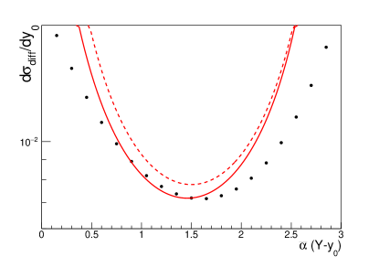
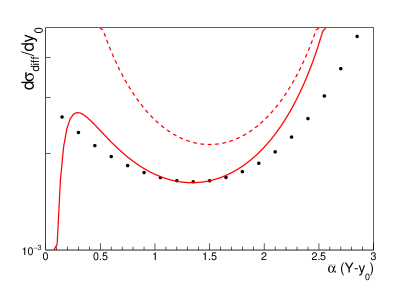
(a)	(b)

Figure 4: Diffractive cross section for $\bar{\alpha}Y=3$ as a function of $\bar{\alpha}(Y-y_{0})$ for two sizes of the onium chosen in the scaling region: (a) $x_{01}=8\times 10^{-4}$, (b) $x_{01}=2\times 10^{-4}$ in units of the inverse McLerran-Venugopalan saturation scale $1/Q_{\text{MV}}$. The points correspond to the values of $Y-y_{0}$ at which the diffractive cross section is computed numerically. The continuous line is the fit of the theoretical formula (40). The dashed line is a graph of the same formula, without the Gaussian suppression factor, and without refitting the parameters. It represents the large-$Y$ asymptotics deeply in the scaling region.

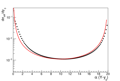
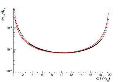
(a)	(b)
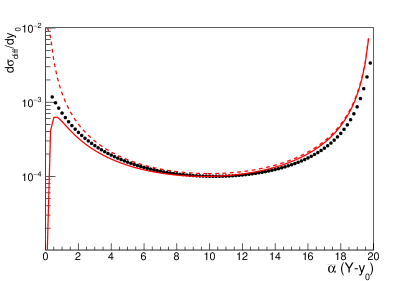
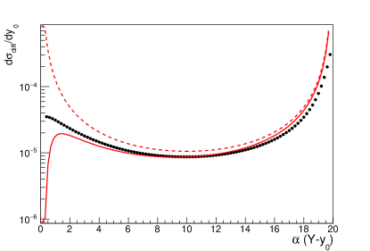
(c)	(d)

Figure 5: The same as in Fig. 4 for $\bar{\alpha}Y=20$ and (a) $x_{01}=10^{-19}$, (b) $x_{01}=10^{-20}$, (c) $x_{01}=10^{-21}$, (d) $x_{01}=10^{-22}$.

We see that our asymptotic formula describes qualitatively the numerical data for $\bar{\alpha}Y=3$. For such a low value of the rapidity, the scaling region is very narrow. Furthermore, the conditions $\bar{\alpha}y_{0}>1$ and $\bar{\alpha}(Y-y_{0})>1$ can obviously not be satisfied with such low values of the rapidity. It is however interesting that although the corrections to the asymptotics are expected to be very large for this choice of the rapidity, the general trend is in agreement with the expectations from the asymptotic formula.

For $\bar{\alpha}Y=20$ (Fig. 5), the numerical data is remarkably well described in the scaling region and on its border. The power law (25) is beautifully seen in the strict scaling region, and the transition to the non-scaling regime is also well described by our theoretical formula (40). One has to keep in mind that it was established under the explicit assumption $\bar{\alpha}Y\gg 1$, and thus is expected to match the regime of asymptotic rapidity only. Note also that again, it is not supposed to be accurate for $\bar{\alpha}y_{0}\sim 1$ or $\bar{\alpha}(Y-y_{0})\sim 1$.

Let us comment on the comparison on our results to the numerical calculation in Ref. [18]. In there, $\sigma_{\text{diff}}$ was computed at fixed $Y$ (set to 10) as a function of $y_{0}$. The dependence upon $y_{0}$ was found close to linear (see Fig. 2 in Ref. [18]), which results in an almost flat dependence of $d\sigma_{\text{diff}}/dy_{0}$ upon $y_{0}$. Since $\bar{\alpha}Y\simeq 2.8$ in that calculation, this is not inconsistent with our results: Indeed, for low rapidities, $d\sigma_{\text{diff}}/dy_{0}$ becomes indeed flatter: Subasymptotic terms screen the asymptotic behavior we have derived here.

4.2 Implementation of a stochastic formulation of diffraction

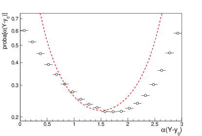
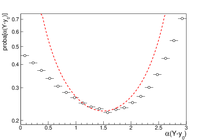
(a)	(b)

Figure 6: Distribution of the rapidity at which the common ancestor split for $\bar{\alpha}Y=3$ and in the scaling region. (a) $x_{01}=5\times 10^{-3}$, (b) $x_{01}=2.5\times 10^{-3}$. The points represent the Monte Carlo calculation as described in the text. The asymptotic prediction (25) is shown (dashed line). The overall normalization is chosen to coincide with the numerical data at $\bar{\alpha}(Y-y_{0})=1.5$.

4.2.1 Procedure

In order to test in a more detailed way our picture of diffraction and its analogy with ancestry problems, we need to set up a definition for a diffractive event in a Monte Carlo approach. This is not straightforward at all because as mentioned in the introductive parts, diffraction is a quantum mechanical phenomenon which may a priori not be defined in purely probabilistic terms.

However, the following procedure is very close to the spirit of the picture we propose. Start with one dipole, evolve it to rapidity $y$ using a Monte Carlo implementation of the dipole model [41, 42]. One obtains a configuration of dipoles, which one replicates once: One copy will build the amplitude, the other one its complex conjugate. We require that these dipoles scatter elastically.

More precisely, each dipole scatters off the nucleus at rest with probability $T_{\text{MV}}$ (or does not scatter with the complementary probability $S_{\text{MV}}=1-T_{\text{MV}}$). We declare that an event is diffractive (or purely elastic) if overall there is at least one dipole which scatters in the amplitude, and at least one dipole in the complex-conjugate amplitude. Now the rapidity gap in that particular event is defined to be the rapidity (counted from the nucleus) at which the common ancestor of all dipoles that scatter split.

A comment is in order. $S$ and $T$ are not probabilities, but probability amplitudes. In our procedure, we trade them for probabilities, which is not rigorously correct. But counting the fraction of events which have at least one interaction in the amplitude and one in the complex-conjugate amplitude is indeed fully equivalent to computing the diffractive cross section using the Good-Walker formula.

4.2.2 Results

Many events are needed in order to arrive at a good statistical accuracy on the rapidity of the common ancestors (about $10^{7}$ realizations of the dipole evolution are in order). In order to lower the complexity and ease the calculation, we simplify the procedure outlined above by replacing the McLerran-Venugopalan amplitude by a sharp $\theta$ function: The dipoles which have a size larger than $1/Q_{\text{MV}}$ interact, the ones that have a size smaller do not, with unit probability in each case. This should be a good approximation since as well-known, the MV amplitude is much steeper than the distribution of dipole sizes generated by the BFKL evolution of the onium. In any implementation of the dipole model, an (unphysical) ultraviolet cutoff is required to regularize the collinear singularity. We choose it to be 10% of the size of the initial onium (which is quite large) in order to keep the number of spectator dipoles reasonable. This has the effect of decreasing the growth of the saturation scale with the rapidity. But we believe that this should not change qualitatively the distribution of common ancestors, since we eventually probe the onium Fock state in size regions which are much larger than this ultraviolet cutoff.

The results are shown in Fig. 6 for $\bar{\alpha}Y=3$. We see that the distribution of the splitting rapidity of the most recent common ancestor follows indeed the same trend as the rapidity gap distribution in Fig. 4, consistently with our picture of diffraction.

5 Conclusion

The main practical result of this paper is a robust prediction for the distribution of the rapidity gaps in diffractive deep-inelastic scattering of a large nucleus at very high energy, see Eq. (25) for the simplest expression, or (21) for an expression which has a wider range of applicability. While the strict asymptotic form we have obtained is probably out of experimental reach, our numerical simulations suggest that the global shape of this distribution may show up already at realistic values of the rapidity, maybe attainable at a future electron-ion collider.

Our main thrust was actually the theoretical understanding of the microscopic mechanism behind high-mass diffractive dissociation phenomena. We have found that the diffractive events were generated by unusually large fluctuations in the partonic evolution of the initial onium. The rapidity $y_{0}$ (when counted from the nucleus) at which they occur determines the size of the gap.

Interestingly enough, the distribution of the rapidity gap size $y_{0}$ has exactly the same form as the distribution of the decay time of the common ancestor of a set of extreme particles in a branching diffusion process. It is actually the mechanism how the common ancestor is singled out in branching random walks which directly motivated our calculation in the context of particle physics. This exciting analogy between a purely probabilistic problem (ancestry in branching random walks) and a process in which quantum mechanics is essential (diffraction) may probably be pushed further. Indeed, the calculation we have performed lead to the same result as Derrida and Mottishaw but is not quite formulated in the same way. The analogy between the ancestry problem and diffraction would deserve more studies.

Among other open problems, taking into account formally subleading effects in the dipole evolution such as the running of the QCD coupling would be in order to be able to appreciate quantitatively how relevant our result is for the phenomenology at a electron-ion collider.

Appendix A Proof that a diffractive event is triggered by a tip fluctuation

The goal of this appendix is to exhibit an argument that when there is (at least) a dipole larger than $1/Q_{s}(y_{0})$ in the onium at rapidity $\tilde{y}_{0}$, it stems predominantly from a front fluctuation (happening, by definition, in the beginning of the evolution) followed by a tip fluctuation occurring precisely at $\tilde{y}_{0}$. We are going to show that earlier fluctuations, at $\tilde{y}_{1}<\tilde{y}_{0}$ which contain dipoles larger than $1/Q_{s}(y_{1})$ cannot generate dipoles of size greater than $1/Q_{s}(y_{0})$ at rapidity $\tilde{y}_{0}$.

In order for a rare fluctuation occurring at rapidity $\tilde{y}_{1}=Y-y_{1}$ (with respect to the onium) to generate offspring in the saturation region at $\tilde{y}_{0}>\tilde{y}_{1}$, it needs to consist in one or a few dipoles of size larger than $1/Q_{s}(y_{1})$ by at least some factor $e^{\delta/2}$, where $\delta$ is a positive number that we shall evaluate soon.

The probability that there be at least one dipole larger than $e^{\delta/2}/Q_{s}(y_{1})$ in the set of dipoles present in the Fock state at rapidity $\tilde{y}_{1}$ solves the BK equation, and thus reads, in the scaling region

$$P(x_{01},\tilde{y}_{1}|e^{\delta/2}/Q_{s}(y_{1}))=c_{P}\ln\frac{e^{\delta}}{x_{\perp}^{2}(\tilde{y}_{1})Q_{s}^{2}(y_{1})}\left[{x_{\perp}^{2}(\tilde{y}_{1})Q_{s}^{2}(y_{1})}\right]^{\gamma_{0}}\\ \times\exp\left\{-\frac{\ln^{2}[x_{\perp}^{2}(\tilde{y}_{1})Q_{s}^{2}(y_{1})]}{2\bar{\alpha}\tilde{y}_{1}\chi^{\prime\prime}(\gamma_{0})}\right\}$$ (41)

(see Eq. (14)) which may be approximated by

$$c_{P}\ln\frac{1}{x_{01}^{2}Q_{s}^{2}(Y)}\left[{x_{01}Q_{s}^{2}(Y)}\right]^{\gamma_{0}}e^{-\gamma_{0}\delta}\left[\frac{\bar{\alpha}Y}{\bar{\alpha}y_{1}\bar{\alpha}\tilde{y}_{1}}\right]^{3/2}\exp\left\{-\frac{\ln^{2}[x_{01}^{2}Q_{s}^{2}(Y)]}{2\bar{\alpha}\tilde{y}_{1}\chi^{\prime\prime}(\gamma_{0})}\right\},$$ (42)

where we have used the same inequality as in Eq. (22) with the replacement $y_{0}\rightarrow y_{1}$, and we have anticipated that the relevant values of $\delta$ will be small compared to $\left|\ln[x_{01}^{2}Q_{s}^{2}(Y)]\right|$.

Let us focus on an event which has its tip at $e^{\delta/2}/Q_{s}(y_{1})$ at the rapidity $\tilde{y}_{1}$. Then at rapidity $\tilde{y}_{0}$, the dipoles at the tip of the front generated by the latter have squared size given typically by the mean position of the tip of a front starting with one dipole at rapidity $\tilde{y}_{1}$ and evolved to rapidity $\tilde{y}_{0}$. It is given by $x_{\perp}^{2}$ in Eq. (15), with the substitutions

$$\tilde{y}\rightarrow\tilde{y}_{0}-\tilde{y}_{1}=y_{1}-y_{0}\quad\text{and}\quad x_{01}^{2}\rightarrow\frac{e^{\delta}}{Q_{s}^{2}(y_{1})}.$$ (43)

The squared size of the largest dipole at rapidity $\tilde{y}_{0}$ thus reads

$$\frac{e^{\delta}}{Q_{s}^{2}(y_{1})}\frac{e^{\bar{\alpha}(y_{1}-y_{0})\chi^{\prime}(\gamma_{0})}}{\left[\bar{\alpha}(y_{1}-y_{0})\right]^{3/2\gamma_{0}}}.$$ (44)

We require that this size be at least as large as $1/Q_{s}^{2}(y_{0})$, which is the condition for having a gap covering a rapidity interval larger than $y_{0}$ in the event. Straightforward algebra leads to the condition $\delta\geq\delta_{0}$, where

$$\delta_{0}\equiv\frac{3}{2\gamma_{0}}\ln\frac{\bar{\alpha}(y_{1}-y_{0})\bar{\alpha}y_{0}}{\bar{\alpha}y_{1}}.$$ (45)

Hence the probability that there be a fluctuation beyond the nuclear saturation boundary at rapidity $\tilde{y}_{1}$ which results in dipoles in the saturation region at $\tilde{y}_{0}$ is $P$ in Eq. (42) with $\delta\rightarrow\delta_{0}$. The ratio of the latter to the probability of finding dipoles in the saturation region at $y_{0}$ reads

$$\frac{P(x_{01},\tilde{y}_{1}|e^{\delta_{0}/2}/Q_{s}(y_{1}))}{P(x_{01},\tilde{y}_{0}|1/Q_{s}(y_{0}))}=\left[\frac{\bar{\alpha}(Y-y_{0})}{\bar{\alpha}(y_{1}-y_{0})\bar{\alpha}(Y-y_{1})}\right]^{3/2}\exp\left\{-\frac{\ln^{2}[x_{01}^{2}Q_{s}^{2}(Y)]}{2\bar{\alpha}(Y-y_{1})\chi^{\prime\prime}(\gamma_{0})}\right\},$$ (46)

when we remain in the scaling region. This expression contains all $y_{1}$-dependent factors of ${P(x_{01},\tilde{y}_{1}|e^{\delta_{0}/2}/Q_{s}(y_{1}))}$.

As the fluctuation may happen at any rapidity between say $y_{0}+\Delta$ and $Y$, a conservative upper bound on the fraction of realizations which contain dipoles larger than $1/Q_{s}(y_{0})$ at $y_{0}$ and dipoles larger than $1/Q_{s}(y_{1})$ at $y_{1}$ with respect to the total number of realizations which have dipoles larger than $1/Q_{s}(y_{0})$ at $y_{0}$ reads

$$R=\int_{\bar{\alpha}(y_{0}+\Delta)}^{\bar{\alpha}Y}d(\bar{\alpha}y_{1})\frac{P(x_{01},\tilde{y}_{1}|e^{\delta_{0}/2}/Q_{s}(y_{1}))}{P(x_{01},\tilde{y}_{0}|1/Q_{s}(y_{0}))}.$$ (47)

We can scale out the factor $[\bar{\alpha}(Y-y_{0})]^{-1/2}$, which is much less than 1 since $y_{0}$ cannot be close to $Y$ by assumption. The change of variable $x=(y_{1}-y_{0})/(Y-y_{0})$ brings the integral into the form

$$R=\frac{1}{\sqrt{\bar{\alpha}(Y-y_{0})}}\int_{\Delta/(Y-y_{0})}^{1}\frac{dx}{x^{3/2}(1-x)^{3/2}}\exp\left\{-\frac{\ln^{2}[x^{2}_{01}Q_{s}^{2}(Y)]}{2\chi^{\prime\prime}(\gamma_{0})\bar{\alpha}(Y-y_{0})(1-x)}\right\}.$$ (48)

The integrand of the remaining integral has two singularities which may potentially enhance the integral, located at the edges of the integration region. The singularity at $y_{1}\rightarrow Y$ results in the following contribution to the integral over $x$ appearing in $R$:

$$\int^{1}\frac{dx}{(1-x)^{3/2}}\exp\left\{-\frac{\ln^{2}[x^{2}_{01}Q_{s}^{2}(Y)]}{2\chi^{\prime\prime}(\gamma_{0})\bar{\alpha}(Y-y_{0})(1-x)}\right\}$$ (49)

The lower bound can be set to $-\infty$, and the integral may then be computed exactly. Inserting the result into the expression of $R$, we get the following contribution:

$$R\xrightarrow[|\ln[x_{01}^{2}Q_{s}^{2}(Y)]|\ll\sqrt{\bar{\alpha}\tilde{y}_{0}\chi^{\prime\prime}(\gamma_{0})}]{}\frac{\sqrt{2\pi\chi^{\prime\prime}(\gamma_{0})}}{\left|\ln[x_{01}^{2}Q_{s}^{2}(Y)]\right|}$$ (50)

which is parametrically small compared to unity by assumption. The contribution of the singularity at $y_{1}\rightarrow y_{0}$ (namely $x\rightarrow 0$) is evaluated in a similar way:

$$R\xrightarrow[\Delta\ll\tilde{y}_{0}]{}\frac{1}{2\sqrt{\bar{\alpha}\Delta}}.$$ (51)

This is of order unity only for $\bar{\alpha}\Delta\sim 1$. This proves that the fluctuations that contribute to the production of dipoles larger than $1/Q_{s}(y_{0})$ at $\tilde{y}_{0}$ happen indeed close to the rapidity $\tilde{y}_{0}$: This is a tip fluctuation.

The reason why this check is crucial to justify our picture and its quantitative form Eq. (18) is the following. According to our discussion in Sec. 2.2.1, if a dipole is produced in the saturation region of the nucleus at rapidity $\tilde{y}_{1}$, then the gap has a size which a priori is at least $y_{1}$. If in the same event there were dipoles in the nuclear saturation region at rapidity $\tilde{y}_{0}$, then this event would count as a diffractive event of gap size exactly equal to $y_{0}$ according to Eq. (18). This would be contradictory, unless $\tilde{y}_{1}\simeq\tilde{y}_{0}$, which is what we have just proven.

References

- [1] Y. V. Kovchegov and E. Levin, Quantum Chromodynamics at High Energy, Cambridge Monogr. Math. Phys. 33 (2012).
- [2] G. Alberi and G. Goggi, Phys. Rept. 74, 1 (1981). doi:10.1016/0370-1573(81)90019-3
- [3] K. A. Goulianos, Phys. Rept. 101, 169 (1983). doi:10.1016/0370-1573(83)90010-8
- [4] C. Bemporad et al., Nucl. Phys. B 33, 397 (1971). doi:10.1016/0550-3213(71)90295-1
- [5] T. Ahmed et al. [H1 Collaboration], Phys. Lett. B 348, 681 (1995) doi:10.1016/0370-2693(95)00279-T [hep-ex/9503005].
- [6] M. Derrick et al. [ZEUS Collaboration], Z. Phys. C 68, 569 (1995) doi:10.1007/BF01565257 [hep-ex/9505010].
- [7] L. Schoeffel, Prog. Part. Nucl. Phys. 65, 9 (2010) doi:10.1016/j.ppnp.2010.02.002 [arXiv:0908.3287 [hep-ph]].
- [8] N. Nikolaev and B. G. Zakharov, Z. Phys. C 53, 331 (1992). doi:10.1007/BF01597573
- [9] W. Buchmuller and A. Hebecker, Phys. Lett. B 355, 573 (1995) doi:10.1016/0370-2693(95)00721-V [hep-ph/9504374].
- [10] A. H. Mueller and B. Patel, Nucl. Phys. B 425, 471 (1994) doi:10.1016/0550-3213(94)90284-4 [hep-ph/9403256].
- [11] A. Bialas and R. B. Peschanski, Phys. Lett. B 378, 302 (1996) doi:10.1016/0370-2693(96)00423-6 [hep-ph/9512427].
- [12] E. Gotsman, E. Levin, M. Lublinsky, U. Maor and K. Tuchin, Phys. Lett. B 492, 47 (2000) doi:10.1016/S0370-2693(00)01020-0 [hep-ph/9911270].
- [13] J. C. Collins, Phys. Rev. D 57, 3051 (1998) Erratum: [Phys. Rev. D 61, 019902 (2000)] doi:10.1103/PhysRevD.61.019902, 10.1103/PhysRevD.57.3051 [hep-ph/9709499].
- [14] K. J. Golec-Biernat and M. Wusthoff, Phys. Rev. D 59, 014017 (1998) doi:10.1103/PhysRevD.59.014017 [hep-ph/9807513].
- [15] M. B. Gay Ducati, E. G. Ferreiro, M. V. T. Machado and C. A. Salgado, Eur. Phys. J. C 24, 109 (2002) doi:10.1007/s100520200911 [hep-ph/0110184].
- [16] Y. V. Kovchegov and E. Levin, Nucl. Phys. B 577, 221 (2000) doi:10.1016/S0550-3213(00)00125-5 [hep-ph/9911523].
- [17] E. Levin and M. Lublinsky, Phys. Lett. B 521, 233 (2001) doi:10.1016/S0370-2693(01)01217-5 [hep-ph/0108265].
- [18] E. Levin and M. Lublinsky, Eur. Phys. J. C 22, 647 (2002) doi:10.1007/s100520100839 [hep-ph/0108239].
- [19] E. Levin and M. Lublinsky, Nucl. Phys. A 712, 95 (2002) doi:10.1016/S0375-9474(02)01269-1 [hep-ph/0207374].
- [20] A. Kovner and U. A. Wiedemann, Phys. Rev. D 64, 114002 (2001) doi:10.1103/PhysRevD.64.114002 [hep-ph/0106240].
- [21] M. Hentschinski, H. Weigert and A. Schafer, Phys. Rev. D 73, 051501 (2006) doi:10.1103/PhysRevD.73.051501 [hep-ph/0509272].
- [22] Y. Hatta, E. Iancu, C. Marquet, G. Soyez and D. N. Triantafyllopoulos, Nucl. Phys. A 773, 95 (2006) doi:10.1016/j.nuclphysa.2006.04.003 [hep-ph/0601150].
- [23] I. Balitsky, Nucl. Phys. B463, 99 (1996), hep-ph/9509348;
- [24] Y. V. Kovchegov, Phys. Rev. D60, 034008 (1999), hep-ph/9901281.
- [25] A. H. Mueller, Nucl. Phys. B 415, 373 (1994).
- [26] L. D. McLerran and R. Venugopalan, Phys. Rev. D 49, 2233 (1994) doi:10.1103/PhysRevD.49.2233 [hep-ph/9309289].
- [27] A. H. Mueller and D. N. Triantafyllopoulos, Nucl. Phys. B 640, 331 (2002) doi:10.1016/S0550-3213(02)00581-3 [hep-ph/0205167].
- [28] S. Munier and R. B. Peschanski, Phys. Rev. Lett. 91, 232001 (2003) doi:10.1103/PhysRevLett.91.232001 [hep-ph/0309177].
- [29] S. Munier and R. B. Peschanski, Phys. Rev. D 69, 034008 (2004) doi:10.1103/PhysRevD.69.034008 [hep-ph/0310357].
- [30] A. M. Stasto, K. J. Golec-Biernat and J. Kwiecinski, Phys. Rev. Lett. 86, 596 (2001) doi:10.1103/PhysRevLett.86.596 [hep-ph/0007192].
- [31] A. H. Mueller and S. Munier, Phys. Lett. B 737 (2014) 303 doi:10.1016/j.physletb.2014.08.058 [arXiv:1405.3131 [hep-ph]].
- [32] J. Bartels, H. Lotter and M. Wüsthoff, Phys. Lett. B 379, 239 (1996) Erratum: [Phys. Lett. B 382, 449 (1996)] doi:10.1016/0370-2693(96)00412-1, 10.1016/0370-2693(96)00840-4 [hep-ph/9602363].
- [33] A. Bialas and R. B. Peschanski, Phys. Lett. B 387, 405 (1996) doi:10.1016/0370-2693(96)01018-0 [hep-ph/9605298].
- [34] A. H. Mueller and S. Munier, Phys. Rev. E 90 (2014) no.4, 042143 doi:10.1103/PhysRevE.90.042143 [arXiv:1404.5500 [cond-mat.dis-nn]].
- [35] B. Derrida and P. Mottishaw, EPL, 115 4 (2016) 40005.
- [36] M. L. Good and W. D. Walker, Phys. Rev. 120 (1960) 1857. doi:10.1103/PhysRev.120.1857
- [37] S. Munier and A. Shoshi, Phys. Rev. D 69 (2004) 074022 doi:10.1103/PhysRevD.69.074022 [hep-ph/0312022].
- [38] B. Derrida and H. Spohn, J. Stat. Phys. 51, 817 (1988).
- [39] S. Munier, Sci. China Phys. Mech. Astron. 58, no. 8, 81001 (2015) doi:10.1007/s11433-015-5666-7 [arXiv:1410.6478 [hep-ph]].
- [40] R. Enberg, K. J. Golec-Biernat and S. Munier, Phys. Rev. D 72 (2005) 074021 doi:10.1103/PhysRevD.72.074021 [hep-ph/0505101].
- [41] G. P. Salam, Comput. Phys. Commun. 105, 62 (1997) [hep-ph/9601220].
- [42] L. Dominé, C. Lorcé, S. Munier and S. Pekar, PoS DIS 2017, 069 (2018) [arXiv:1705.06584 [hep-ph]]; Idem and G. Giacalone, to appear (2018).