A Study of the Point Spread Function in SDSS Images

Abstract

We use SDSS imaging data in $ugriz$ passbands to study the shape of the point spread function (PSF) profile and the variation of its width with wavelength and time. We find that the PSF profile is well described by theoretical predictions based on von Kármán’s turbulence theory. The observed PSF radial profile can be parametrized by only two parameters, the profile’s full width at half maximum (FWHM) and a normalization of the contribution of an empirically determined “instrumental” PSF. The profile shape is very similar to the “double gaussian plus power-law wing” decomposition used by SDSS image processing pipeline, but here it is successfully modeled with two free model parameters, rather than six as in SDSS pipeline. The FWHM variation with wavelength follows the $\lambda^{\alpha}$ power law, where $\alpha\approx-0.3$ and is correlated with the FWHM itself. The observed behavior is much better described by von Kármán’s turbulence theory with the outer scale parameter in the range 5–100 m, than by the Kolmogorov’s turbulence theory. We also measure the temporal and angular structure functions for FWHM and compare them to simulations and results from literature. The angular structure function saturates at scales beyond 0.5$-$1.0 degree. The power spectrum of the temporal behavior is found to be broadly consistent with a damped random walk model with characteristic timescale in the range $\sim 5-30$ minutes, though data show a shallower high-frequency behavior. The latter is well fit by a single power law with index in the range $-1.5$ to $-1.0$. A hybrid model is likely needed to fully capture both the low-frequency and high-frequency behavior of the temporal variations of atmospheric seeing.

1 Introduction

The atmospheric seeing, the point-spread function (PSF) due to atmospheric turbulence, plays a major role in ground-based astronomy (Roddier, 1981). An adequate description of the PSF is critical for photometry, star-galaxy separation, and for unbiased measures of the shapes of nonstellar objects (Lupton et al., 2001). In addition, better understanding of the PSF temporal variation can lead to improved seeing forecasts; for example, such forecasts are considered in the optimization of LSST observing strategy (Ivezić et al., 2008).

Seeing varies with the wavelength of observation, and it also varies with time, on time scales ranging from minutes to years. These variations, as well as the radial seeing profile, can be understood as manifestations of atmospheric instabilities due to turbulent layers. Although turbulence is a complex physical phenomenon, the basic properties of the atmospheric seeing can be predicted from first principles (Racine, 2009). The von Kármán turbulence theory, an extension of the Komogorov theory that introduces a finite maximum size for turbulent eddies (the so-called outer scale parameter), quantitatively predicts the seeing profile and the variation of seeing with wavelength (Borgnino, 1990; Ziad et al., 2000). Therefore, seeing measurements can be used to test the theory and estimate the relevant physical parameters.

An unprecedentedly large high-quality database of seeing measurements was delivered by the Sloan Digital Sky Survey (SDSS, York et al. 2000), a large-area multi-bandpass digital sky survey. The SDSS delivered homogeneous and deep ($r\lesssim 22.5$) photometry in five bandpasses ($u$, $g$, $r$, $i$, and $z$, with effective wavelengths of 3551, 4686, 6166, 7480, and 8932 $\AA$), accurate to about 0.02 mag for unresolved sources not limited by photon statistics (Sesar et al., 2007). Astrometric positions are accurate to better than 0.1 arcsec per coordinate for sources with $r<20.5$ (Pier et al., 2003), and the morphological information from the images allows reliable star-galaxy separation to $r<21.5$ (Lupton et al., 2002).

The SDSS camera (Gunn et al. 1998) used drift-scanning observing mode (scanning along great circles at the sidereal rate) and detected objects in the order $r$-$i$-$u$-$z$-$g$, with detections in two successive bands separated in time by 72 s. Each of the six camera columns produces a 13.5 arcmin wide scan; the scans are split into “fields” 9.0 arcmin long, corresponding to 36 seconds of time (the exposure time is 54.1 seconds because the sensor size is 2k by 2k pixels, with 0.396 arcsec per pixel). The point-spread function (PSF) is estimated as a function of position within each field, although we only use one estimate per field, and in each bandpass - there are about 148 seeing estimates for each square degree of scanned sky. As a result, the SDSS measurements can be used to explore the seeing dependence on time (on time scales from 1 minute to 10 hours) and wavelength (from the UV to the near-IR), as well as its angular correlation on the sky on scales from arcminutes to about 2.5 degrees. Thanks to large dynamic range for stellar brightness, the PSF can be traced to large radii ($\sim$30 arcsec) and compared to seeing profiles predicted by turbulence theories.

The SDSS seeing measurements represent an excellent database that has not yet been systematically explored. Here we utilize about a million SDSS seeing estimates to study the seeing profile and its behavior as a function of time and wavelength, and compare our results to theoretical expectations. The outline of this paper is as follows. In §2, we give a brief description of the observations and the data used in analysis. We describe the PSF profile analysis, including estimation method for the full-width-at-half-maximum (FWHM) seeing parameter, in §3. In §4, we analyse the dependence of FWHM on wavelength, and its angular and temporal structure functions. We present and discuss our conclusions in §5.

2 Data Overview

We describe here the SDSS dataset and seeing estimates used in this work. The selected subset of data, the so-called Stripe 82, represents about one third of all SDSS imaging data.

2.1 Stripe 82 dataset

The equatorial Stripe 82 region (22^h24^m $<$ R.A. $<$ 04^h08^m, $-$1.27^∘ $<$ Dec $<$ $+$1.27^∘, about 290 deg²) from the southern Galactic cap ($-64^{\circ}<b<-20^{\circ}$) was repeatedly imaged (of order one hundred times) by SDSS to study time-domain phenomena (such as supernovae, asteroids, variable stars, quasar variability). An observing stretch of SDSS imaging data is called a “run”. Often there is only a single run for a given observing night, though sometimes there are multiple runs per night. In this paper we use seeing data for 108 runs, with a total of 947,400 fields, obtained between September, 1998 and September 2008 (there are 6 camera columns, each with 5 filters; for more details please see Gunn et al. 2006). All runs are obtained during the Fall observing season (September to December). Astrometric and photometric aspects of this dataset have been discussed in detail by Ivezić et al. (2007) and Sesar et al. (2007).

2.2 The treatment of seeing in SDSS

Even in the absence of atmospheric inhomogeneities, the SDSS telescope delivers images whose FWHMs vary by up to 15% from one side of a CCD to the other; the worst effects are seen in the chips farthest from the optical axis (Gunn et al., 2006). Moreover, since the atmospheric seeing varies with time, the delivered image quality is a complex two-dimensional function even on the scale of a single field (for an example of the instantaneous image quality across the imaging camera, see Figure 7 in Stoughton et al. 2002).

The SDSS imaging PSF is modeled heuristically in each band using a Karhunen-Loéve (K-L) transform (Lupton et al., 2002). Using stars brighter than roughly 20^th magnitude, the PSF images from a series of five fields are expanded into eigenimages and the first three terms are kept (K-L transform is also known as the Principal Component Analysis). The angular variation of the eigencoefficients is fit with polynomials, using data from the field in question, plus the immediately preceding and following half-fields. The success of this K-L expansion is gauged by comparing PSF photometry based on the modeled K-L PSFs with large-aperture photometry for the same (bright) stars (Stoughton et al., 2002). Parameters that characterize seeing for one field of imaging data are stored in the so-called psField files. The status parameter flag for each field indicates the success of the K-L decomposition.

In addition to the K-L decomposition, the SDSS processing pipeline computes parameters of the best-fit circular double Gaussian, evaluated at the center of each field. The measured PSF profiles are extended to $\sim$30 arcsec using observations of bright stars and at such large radii double Gaussian fits underpredict the measured profiles. For this reason, the fits are extended to include the so-called “power-law wings”, which is reminiscent of the Moffat function,

$$PSF(r)={\exp(-{r^{2}\over 2\,\sigma_{1}^{2}})+b\,\exp(-{r^{2}\over 2\,\sigma_{2}^{2}})+p_{0}\left(1+{r^{2}\over\beta\sigma_{P}^{2}}\right)^{-\beta/2}\over 1+b+p_{0}}.$$ (1)

The measured PSFs are thus modeled using 6 free parameters ($\sigma_{1}$, $\sigma_{2}$, $\sigma_{P}$, $b$, $p_{0}$ and $\beta$), and the best-fit parameters are reported in the psField files. Given that the measured profiles include only up to 10 data points, the fits are usually excellent although they do not appear very robust (for examples of bad fits see Fig. 2).

3 The PSF profile analysis

Since the complex 6-parameter PSF fit given by Eq. (1) was adopted by the SDSS processing pipeline, significant progress has been made in validating the von Kármán model of the atmosphere and measuring the associated outer scale (see, for example, Tokovinin 2002, Boccas 2004, and Martinez et al. 2010). In this section, we describe our much simpler 2-parameter fits to the SDSS PSF radial profiles using the von Kármán atmosphere model.

The seeing profile predicted by the von Kármán atmosphere model is a two-parameter family that can be parametrized by the FWHM and the so-called outer scale parameter. The Kolmogorov seeing profile is a special case of the von Kármán seeing with the infinitely large outer scale. The radial profiles of the von Kármán PSF with a few different values of outer scale are shown in Fig. 1 (a). In Fig. 1 (c), the profiles with finite outer scales ($L_{0}$) are normalized to the Kolmogorov profile.

Our fitting of each PSF radial profile is a 2-step process. First we fit the measured PSF profile to a von Kármán PSF with only one free parameter - the FWHM of the von Kármán profile, while a fiducial outer scale of 30 meters is assumed fixed. As discernible from Fig. 1 (a) and (c), the impact of the exact value of $L_{0}$ on the profile shape is small. A fixed value of $L_{0}$ induces a small systematic uncertainty in the normalization of the contribution of instrumental PSF, discussed in § 3.1 below. The von Kármán PSF profile is generated by creating the atmosphere structure function first, as given by Eq. (18) in Tokovinin (2002), then calculating the PSF through the Optical Transfer Function. Pixel integration is taken into account by a factor of 10 oversampling.

Ideally, the Fried parameter $r_{0}$ would be used as the free parameter in the fit to the von Kármán model. However, that would require us to calculate the special functions and do the Fourier Transform on a large array for each function evaluation. Instead, we opted to generate a single von Kármán PSF template with the FWHM of 1.0 arcsec. In our one-parameter von Kármán fit, we only stretch or compress the template radially to get the best match with the data, in the least-square sense. Fig. 1 (b) shows a comparison of three PSF profiles, one generated with FWHM of 1.0 arcsec, the other two generated with FWHM of 0.5 and 2.0 arcsec, respectively, then stretched and compressed to 1.0 arcsec. The three curves are seen to be almost indistinguishable. Fig. 1 (d) shows the same three profiles when normalized to the one generated with FWHM of 1.0 arcsec.

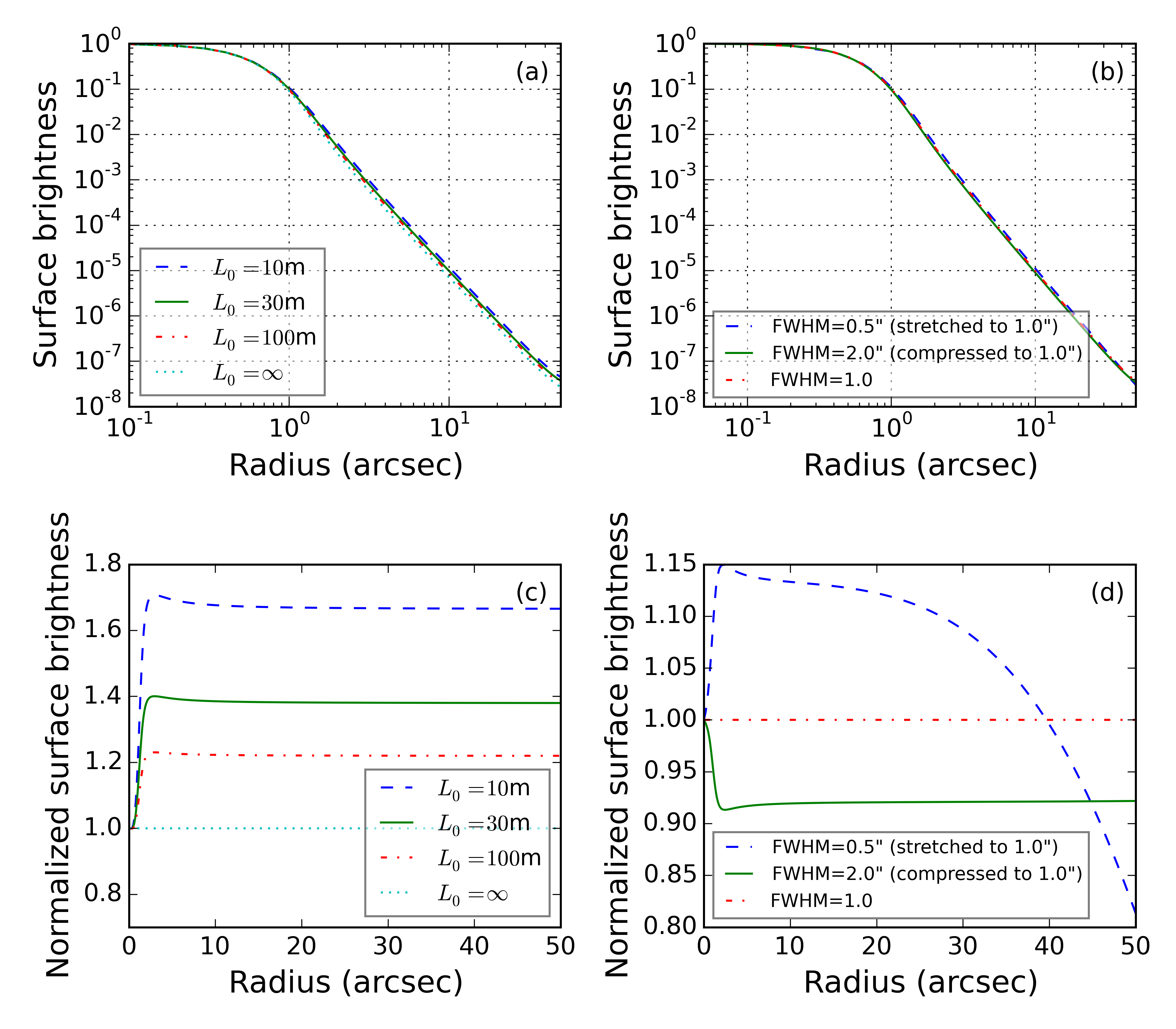
Figure 1: PSF radial profiles with the von Kármán model for a few different outer scale ($L_{0}$) values (left) and $r_{0}$ values (right). All profiles have FWHM of 1.0 arcsec, and are normalized to unit peak intensity. The von Kármán model becomes Kolmogorov when $L_{0}=\infty$. In the right plot, the dashed and dotted profiles are created with $L_{0}=30$m, and FWHM of 0.5 arcsec and 2.0 arcsec, respectively, then stretched and compressed to 1.0 arcsec.

The $\chi^{2}$ is defined using the first four data points on the measured radial profiles, at 0.16, 0.51, 0.87 and 1.44 arcsec, respectively. These points correspond to highest photon counts, and also are least susceptible to errors in the background brightness estimates. The error estimates on these data points come from the original SDSS measurements.

Although the fitted curves agree with the input data points very well, generally much better than the original 6-parameter double-Gaussian fit by SDSS, they do not always describe the PSF tail beyond $\sim 15$ arcsec radius. Some examples of such fits are shown in Fig. 2. This discrepancy is easily understood because the PSF tails in the optical bands can be different due to the properties of the CCDs. The SDSS $u$-, $g$-, $r$-, and $z$-bands differ only slightly due to changing conversion depth. It is known that the $i$-band PSF has “stronger tails” because of scattering in the CCD (J.E. Gunn, priv. comm.). The Si is transparent at long $i$-band wavelengths so light goes all the way through the chip and is reflected off the solder, and passes back up through the Si. This effect is not visible in the $z$-band because in this case thick front-side illuminated chips are used (in all other bands, thin back-side chips are used).

3.1 Instrumental PSF

To improve the fit quality at large radii, in the second fitting step we introduce an empirical “instrumental” PSF. Despite the name, this component might also include effects not modeled by the von Kármán theory, such as aerosol scattering in the atmosphere, dust on the mirrors, and scattering in the CCDs. The observed PSF can be expressed as a convolution of the atmosphere, represented by the von Kármán, and the instrumental PSF,

$$\textrm{PSF}=\textrm{vonK}(\textrm{FWHM})\otimes\textrm{PSF}_{\textrm{inst}},$$ (2)

where vonK is the von Kármán shape, whose only parameter, FWHM, is fixed to the value from step one. Fig. 2 shows that the tails of the PSF can be well described using a second order polynomial in the logarithmic space of the intensity. Meanwhile, since $\textrm{PSF}_{\textrm{inst}}$ is a convolution kernel, we can use a narrow Gaussian to describe its central core. We define the functional form of the instrumental PSF as

$$\textrm{PSF}_{\textrm{inst}}=\exp(-\frac{r^{2}}{2\sigma^{2}})+10^{p(r)},$$ (3)

where $p(r)$ is a second order polynomial. The standard deviation of the Gaussian, $\sigma$, cannot be too wide because the von Kármán term already well describes the core of the PSF. We found that $\sigma=0.1$ arcsec is an acceptable choice.

We define the second order polynomial $p$ as

$$p(r)=\eta(ar^{2}+br+1).$$ (4)

Because the shape of the instrumental PSF tail should not vary with time, but does vary with the filter and camera column, we determine the values of $a$ and $b$ for each band-camera-column combination using one representative field, then fix them at those values for all step-two fits. For each SDSS PSF radial profile, these one-time least-square fits use all the data points with radii up to $\sim$30 arcsec. Each fit has $a$, $b$, and $\eta$ as free parameters, and involves a 2-dimensional convolution (see Eq. 2), The fits are very slow but need to be done only once. We used here run 94, field 11 for these one-time fits, but verified that the results are stable for other choices of run and field. The best-fit values of $a$ and $b$ are listed in Table 1.

For step-two PSF fitting, parameters $a$ and $b$ are fixed for each band-camera-column combination. $\eta$, the relative normalization of the instrumental PSF tail in the logarithm-space, is the only free parameter. This second fitting step is also a least-square fit with a 2-dimensional convolution, using all the data points with radii up to $\sim$30 arcsec. Each two-step PSF fit can be done in a few seconds. Fig. 2 shows the results of our PSF fits from run 4874. The two-parameter fits describe the PSF radial profiles quite well, both in the core and in the tails. The addition of the instrumental PSF (dot-dashed lines in Fig. 2) significantly improves the fit quality, especially in the $i$-band. Its impact on the encircled energy profile is shown in Fig. 3.

Fig. 2 also shows the original SDSS “double Gaussian plus power-law wing” fits, described by Eq. 1. They sometimes fail catastrophically; our analysis revealed two kinds of failures: one case is characterized by $p_{0}=10^{-7}$ and another by $\beta$=3 or 10. For the sample of 947,400 PSF fits analyzed here, each failure case occurs with a frequency of about 12%. Inspection of the SDSS code (findPsf.c) reveals that these values signal bad fits which did not converge for various (unknown) reasons.

There are a total of 108 runs in the SDSS Stripe 82 dataset. Among them, run 4874 is the longest, with 981 fields. In the rest of this paper, whenever we illustrate results from a single run, we always use run 4874 as the fiducial example run.

Table 1: Values for instrumental PSF shape parameters $a$ and $b$.

		Camera Column
		1	2	3	4	5	6
	a($\times 10^{-4}$)	$-$4.4	$-$4.4	$-$1.9	$-$4.4	$-$4.4	$-$4.4
$u$	b($\times 10^{-2}$)	3.3	3.3	1.3	4.7	4.7	4.7
	a($\times 10^{-4}$)	$-$5.3	$-$5.3	$-$4.4	$-$4.4	$-$5.3	$-$5.3
$g$	b($\times 10^{-2}$)	3.5	3.5	3.3	3.3	3.5	3.5
	a($\times 10^{-4}$)	$-$4.9	$-$4.9	$-$4.9	$-$5.8	$-$4.4	$-$4.4
$r$	b($\times 10^{-2}$)	3.1	3.1	3.1	3.3	3.3	3.3
	a($\times 10^{-4}$)	$-$1.3	$-$2.2	$-$1.3	$-$1.3	$-$1.8	-0.4
$i$	b($\times 10^{-2}$)	1.7	1.8	1.7	1.7	1.7	1.5
	a($\times 10^{-4}$)	$-$6.2	4.4	$-$6.2	$-$4.4	$-$6.2	$-$4.4
$z$	b($\times 10^{-2}$)	4.0	2.0	4.0	3.1	4.4	4.7

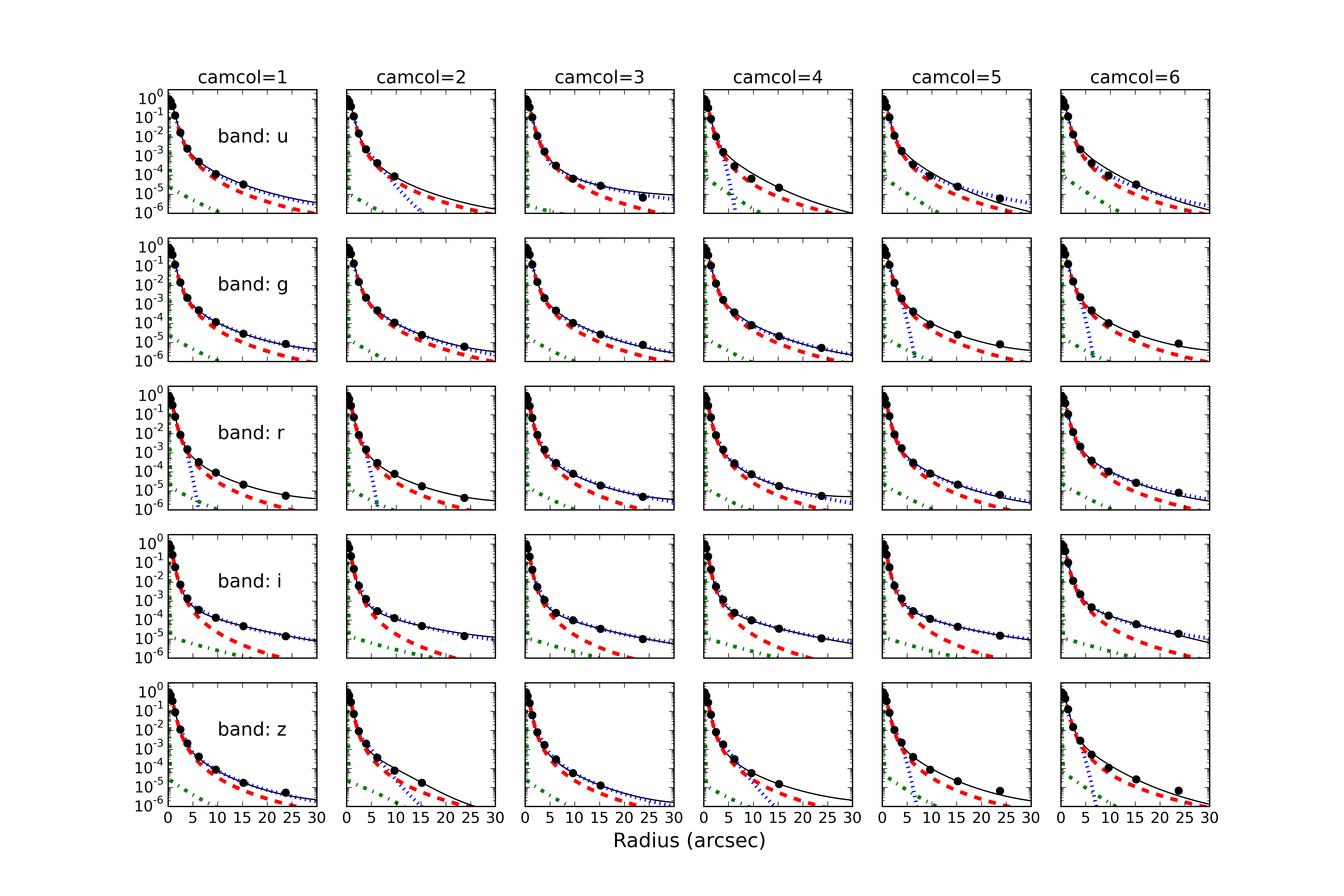
Figure 2: Fits to the PSF radial profiles from run 4874, field 121. Symbols are SDSS data. Red dashed curves are the best one-parameter von Kármán fits. Black solid curves are the red curve convolved with the instrumental PSF (green dot-dashed lines), where the scaling factor (relative normalization) for the tail component is allowed to vary. As a reference, the original “SDSS double Gaussian plus power-law wing” fits, described by eq. 1, are shown in blue dotted lines – they sometimes fail catastrophically (see text). Note that the y-axis is shown on the logarithmic scale.

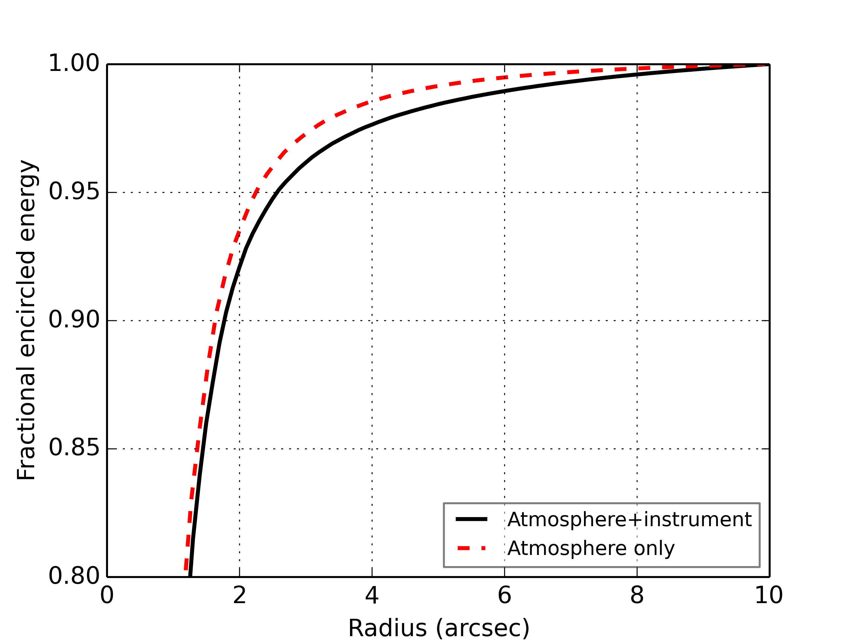
Figure 3: Encirlced energy distributions for PSF profiles from run 4874, field 121, $r$-band, camera column 3. The black solid curve is for the delivered PSF with contributions from atmosphere and instrument. The red dashed curve is for atmosphere only.

4 The analysis of FWHM behavior

Given that the observed seeing is by and large described by a single parameter, FWHM, we study here three aspects of its variation in detail: dependence on wavelength, the spatial (angular) structure function, and temporal behavior. We note that details about the seeing profile tails, including the contribution of the instrumental profile and the $i$ band behavior, do not matter here because we focus only on the FWHM behavior.

4.1 The FWHM dependence on wavelength

The Kolmogorov turbulence theory gives a standard formula for the FWHM of a long-exposure seeing-limited PSF in a large telescope,

$$\textrm{FWHM}^{\rm Kolm}(\lambda,X)=\frac{0.976\lambda}{r_{0}(\lambda,X)},$$ (5)

$$r_{0}(\lambda,X)=r_{0}(\lambda_{0},1)\left(\frac{\lambda}{\lambda_{0}}\right)^{1.2}\frac{1}{X^{0.6}},$$ (6)

where $\lambda$ is the wavelength in meter, $X$ is the airmass, $r_{0}$ is the Fried parameter in meter, and $\textrm{FWHM}^{\rm Kolm}$ is in radian. We use $\lambda_{0}$ as the reference wavelength. $r_{0}(\lambda_{0},1)$ is the $r_{0}$ for $\lambda=\lambda_{0}$ and $X$=1. Substituting Eq. (6) into (5), it is easy to show that

$$\textrm{FWHM}^{\rm Kolm}\propto\lambda^{-0.2}.$$ (7)

With the von Kármán atmosphere model, the FWHM as in Eq. (5) needs an additional correction factor which is a function of the outer scale $L_{0}$ (Tokovinin, 2002),

$$\textrm{FWHM}^{\rm vonK}(\lambda,X)=\frac{0.976\lambda}{r_{0}(\lambda,X)}\sqrt{1-2.183\left(\frac{r_{0}(\lambda,X)}{L_{0}}\right)^{0.356}}.$$ (8)

If a power-law approximation is attempted,

$$\textrm{FWHM}^{\rm vonK}\propto\lambda^{\alpha},$$ (9)

$\alpha$ becomes a function of $L_{0}$ and $r_{0}$ at a specified wavelength and airmass, or equivalently, a function of $L_{0}$ and FWHM^vonK. For the subsequent analysis, we adopt the $r$ band as the fiducial band (with the effective wavelength of 616.6 nm).

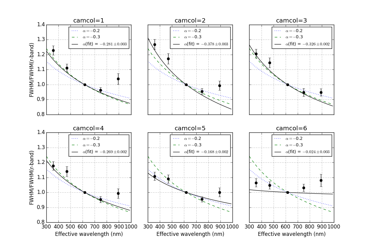
Figure 4: The behavior of FWHM as a function of wavelength for the fiducial run 4874. Symbols are SDSS data and solid line is the best power-law fit, with the best-fit slope ($\alpha$) shown in inset. For comparison purposes, the $\alpha=-0.2$ (dotted) and $\alpha=-0.3$ (dashed) lines are also shown. For the ensemble behavior of best-fit $\alpha$, see Fig. 5.

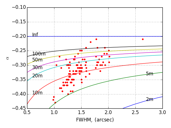
Figure 5: The variation of the best-fit power-law index for the wavelength dependence of FWHM, $\alpha$, vs. the FWHM in the $r$-band for all the 108 Stripe 82 runs. The symbols are SDSS measurements of $\alpha$ based on the $ugri$ data and averaged over camera columns 2 to 5. The curves are predictions of the von Kármán model, with $L_{0}$ ranging from 2 meters to infinity, as labeled. The data are clearly inconsistent with Kolmogorov predictions ($L_{0}=\infty$) and reasonably well described by von Kármán model and $L_{0}$ in the range from 5m to $\sim$100m.

For each run from SDSS Stripe 82 data, and each camera column, we make a least-square fit to all the simultaneous FWHM measurements across the optical bands, to estimate the power-law index $\alpha$ (see Eq. 9). The errors on the FWHM measurements in each optical band comes from averaging over all the fields. All FWHM values are multiplied by $1/X^{0.6}$ to correct for the airmass effects.

All FWHM are normalized using corresponding FWHM in the $r$-band taken at the same moment in time. We take into account that the same field number does not correspond to the same time in all filters. The scanning order in the SDSS camera is $r$-$i$-$u$-$z$-$g$, with the delay between the two successive filters corresponding to 2 fields. That is, if we take the field number $F$ for the $r$-band, then we need to take FWHM for the $i$-band from field $F-2$, for the $u$-band from $F-4$, and so on.

Fig. 4 shows such fits for run 4874. Significant deviation from $\alpha=-0.2$, predicted by the Kolmogorov model, can be seen in most bands. We find that fits in columns 1-5 are always similar, while in column 6 the slope is systematically lower. Similarly, the data in the $ugri$ bands are well fit by the power law, while the $z$ band the data are systematically larger than the power-law fit. For this reason, we refit the data using only $ugri$ bands and average results without using the edge columns (1 and 6, though including column 1 does not substantially change the results). Fig. 5 shows a scatter plot of the resulting best-fit $\alpha$ vs. the FWHM in the $r$-band, for all the analyzed runs.

As discussed above, according to the von Kármán atmosphere model, the power index $\alpha$ should be a function of the outer scale $L_{0}$ and FWHM. A correlation between $\alpha$ and the FWHM is discernible in Fig. 5. Similar correlations have been seen in Subaru images and reported by Oya et al. (2016). The data points are overlaid with curves predicted by the von Kármán model, with $L_{0}$ varying from 2 m to infinity. The data clearly deviate from the Kolmogorov model prediction, which is the horizontal line at $\alpha=-0.20$, with an infinite $L_{0}$. For example, for LSST’s fiducial FWHM of 0.6 arcsec and the commonly assumed $L_{0}=30$ m, the von Kármán model predicts an $\alpha$ value close to $-0.31$.

4.2 Angular structure function

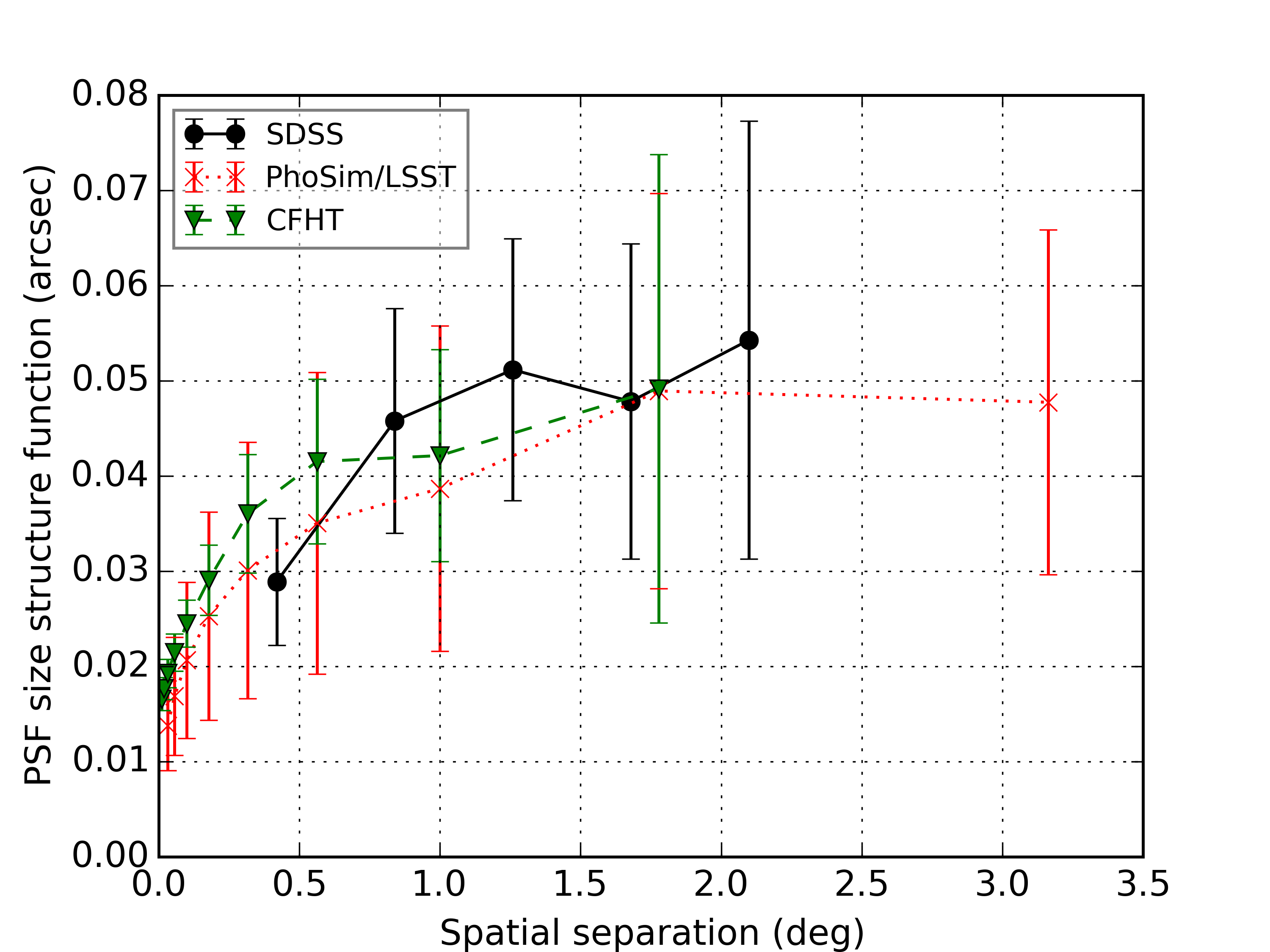
Figure 6: The angular structure function for the PSF size determined using CFHT data from Heymans et al. (2012), SDSS data analyzed here, and LSST image simulations. SDSS measurements are averaged over 86 runs with the number of fields larger than 100.

To examine the angular (spatial) correlation of the FWHM, we compute the angular structure function using PSF measurements from all 6 camera columns. Our structure function is defined as the root-mean-square scatter of the PSF size differences of pairs of stars in the same distance bin along the direction perpendicular to the scanning direction . The SDSS curves are combined for 86 Stripe 82 runs with the number of fields larger than 100 (out of 108 runs) We also compared the structure functions for each band separately, with and without camera columns 1 and 6, and found no statistically significant differences. Results for the $r$-band are shown in Fig. 6.

The structure function starts saturating at separations of $\sim 0.5-1.0$ degree, with an asymptotic value of about $\sim 0.05$ arcsec. In other words, the seeing rms variation at large angular scales is about 5%, but we emphasize that our data do not probe scales beyond 2.5 degree.

For comparison, Fig.  6 also shows results from the CFHT PSF measurements (Heymans et al., 2012), and simulated PSF angular structure functions obtained using image simulation code PhoSim (Peterson et al., 2015). The PhoSim PSF profiles are obtained by simulating a grid of stars spaced by 6 arcminutes with non-perturbed LSST telescope and ideal sensors. The results are averaged over 9 different atmosphere realizations with different wind and screen parameters and airmass, and over 3 different wavelengths (350 nm, 660 nm, and 970 nm). The CFHT PSF size measurements were made in the $i$-band, and provided by the authors of Heymans et al. (2012). The three curves in Fig. 6 appear to be quantitatively consistent with each other, even though they correspond to telescopes at different sites and with different optics.

We note that the PhoSim code could be used to further quantitatively study the variation of seeing with outer scale and the impact of telescope diameter; however, such detailed modeling studies are beyond the scope of this report.

4.3 Temporal behavior

4.3.1 Power spectrum analysis

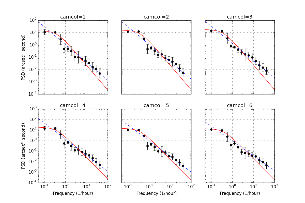
Figure 7: PSF size temporal power spectral density for run 4874, r-band. The solid lines are fits using the damped random walk model. The dashed lines show best fits based on a single power law. The former predicts a steeper high-frequency behavior, while the latter cannnot explain the turnover at low frequencies.

To study the temporal behavior of the seeing, we first analyze its power spectrum. Fig. 7 shows the temporal power spectral density (PSD) of the PSF FWHM for 6 camera columns, in run 4874, $r$-band. The time difference between subsequent fields is 36 seconds. Even though anormalies on the wavelength dependence of the FWHM are seen in column 6, it is clear from Fig. 6 that the temporal behavior of the FWHM does not vary with band. The temporal analysis presented in this section includes all the camera columns and all the optical bands. We have repeated the analysis without using FWHM measurements from $z$-band and camera columns 1 and 6, and found no statistically significant differences in results.

We fit the PSD using two competing models. The first is a damped random walk (DRW) model (for introduction see Chapter 10 in Ivezić et al., 2014),

$$\textrm{PSD}(f)=\frac{\tau^{2}SF^{2}_{\infty}}{1+(2\pi f\tau)^{2}},$$ (10)

where $f$ is the temporal frequency, $SF_{\infty}$ is the asymptotic value of the structure function, and $\tau$ is the characteristic timescale. The solid curves in Fig. 7 show fits using this model, with $f$, $\tau$, and $SF_{\infty}$ as free parameters. Note that due to the lack of data toward the low-frequency end, the first and second bins are four and two times wider than the rest of the bins, respectively. Combining fit results for all camera columns and optical bands for run 4874 gives $\tau=23.6\pm 1.3$ minutes. Making the same fits for all the 108 runs in Stripe 82, we obtain the $\tau$ distribution vs. the duration of each run, as shown in Fig. 8 (left). The shorter runs tend to give smaller timescale. It is plausible that short runs cannot reliably constrain $\tau$ due to the lack of data toward the low-frequency end of the spectra. There are 12 runs longer than 6 hours and their characteristic timescales are within the range of about $\sim 5-30$ minutes. This result is generally consistent with  Racine (1996), where a timescale of $\tau=17\pm 1$ minutes was found.

The data consistently show a shallower high-frequency behavior than predicted by damped random walk ($\propto 1/f^{2}$). In order to quantitatively describe the high-frequency tail of the PSD, we fit a simple power law,

$$\textrm{PSD}(f)=Bf^{\beta},$$ (11)

where $B$ is the normalization factor, and $\beta$ is the power-law index. Best-fits are illustrated for run 4874 are in Fig. 7 (dashed lines). Combining fit results for all camera columns and filters gives $\beta=-1.29\pm 0.09$ for run 4874. Making the same fits for all the 108 runs in Stripe 82, we obtained the $\beta$ distribution vs. the duration of each run shown in Fig. 8 (right). The shorter runs give $\beta$ values with a larger variance, but nevertheless it is clear that for most runs the high-frequency behavior can be described with a power-law index in the range $-1.5$ to $-1.0$. We note that Snyder et al. (2016) measured steeper slopes, though at much higher frequencies. On the other hand, a single power law cannot explain the turnover at low frequencies.

Therefore, neither model provides a satifactory fit over the entire frequency range: the power law fit systematically over predicts the low-frequency part of the PSD, while the $1/f^{2}$ high-frequency behavior of damped random walk model is too steep. It is likely that a hybrid model would work, for example, a simple generalization of the random walk model (see Eq. (19) in Dunkley et al. (2005)),

$$\textrm{PSD}(f)=\frac{\tau^{\alpha}SF^{2}_{\infty}}{1+(2\pi f\tau)^{\alpha}}.$$ (12)

Performing fits to our data using this model did not yield useful results on the characteristic timescale, due to our lack of data points at low frequency, and therefore the incapability in constraining one additional parameter ($\alpha$ in Eq. (12)). We leave more detailed analysis, perhaps informed by the PhoSim modeling, for future work.

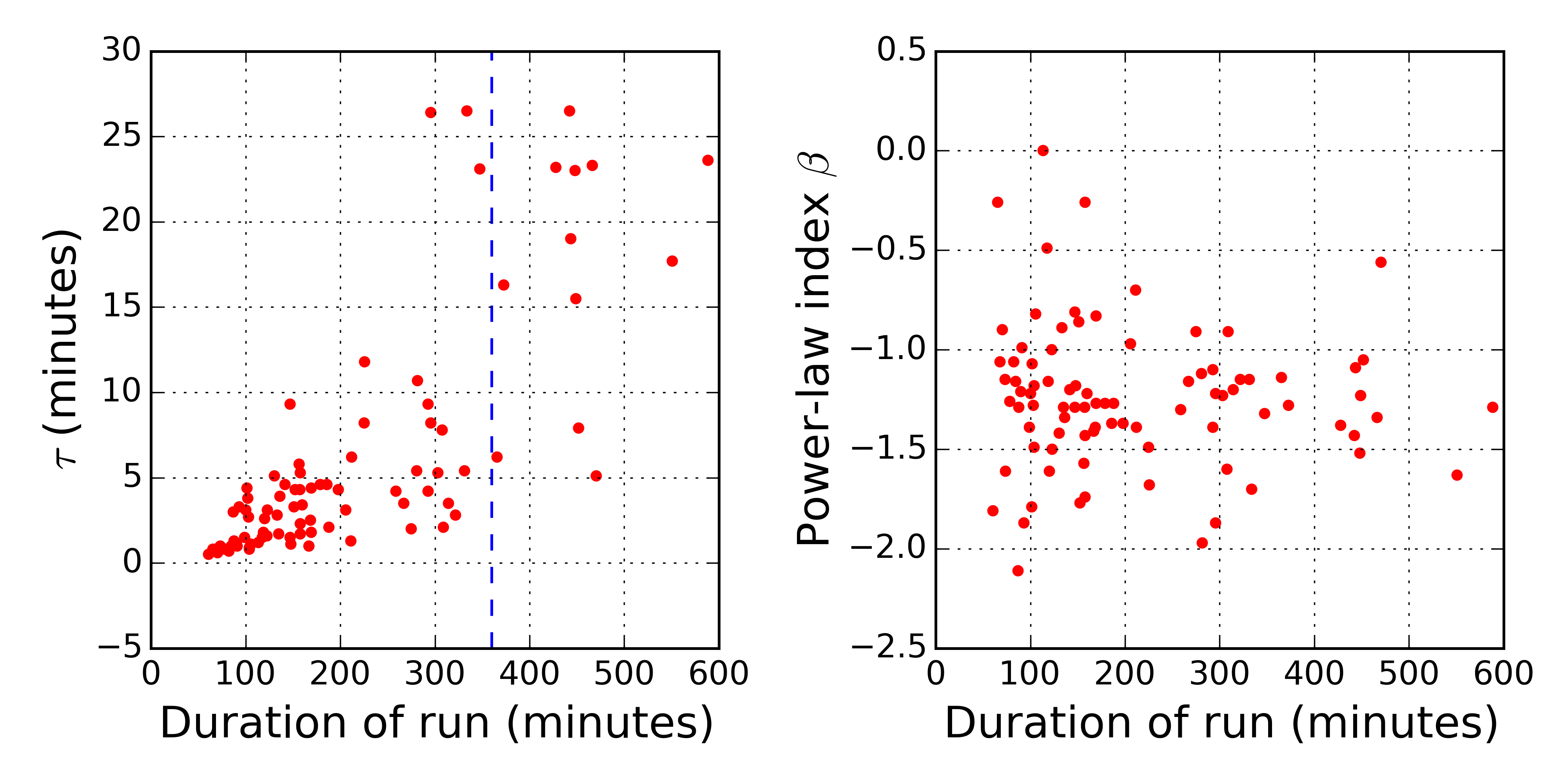
Figure 8: Left: The symbols show the best-fit characteristic timescale $\tau$ in damped random walk for all 108 runs in Stripe 82 vs. the duration of each run. It is plausible that short runs cannot reliably constrain $\tau$. The vertical dashed line indicates run duration of 6 hours. Right: The power-law index $\beta$ for a single power law fit for all 108 runs vs. the duration of each run. Note that for the majority of runs, $\beta$ is larger than the value appropriate for damped random walk ($\beta=-2$).

4.3.2 Structure function analysis

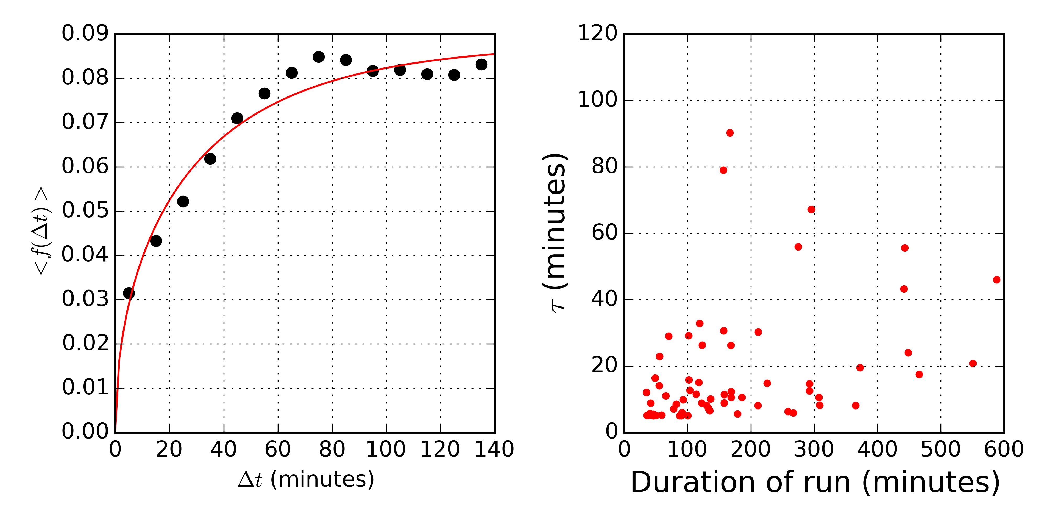
Figure 9: Left: The average normalized seeing difference, $<f(\Delta t)>$, as a function of the time separation, $\Delta t$, for run 4874, camera column 1, in the $r$-band. The fit to Eq. (14) gives $f(\Delta t)^{\infty}=0.088\pm 0.005$, $\tau=45.1\pm 10.3$ minutes and $\gamma$ = 1.016$\pm$0.102. A damped random walk model has $\gamma=1$. Right: The timescale $\tau$ vs. the duration of each run. Note that for most runs $\tau$ is in the range 5-30 minutes (runs shorter than 20 minutes or where the fitted $\tau$ is longer than 2/3 of the duration of the run are left out).

An alternative approach to power spectrum analysis is offered by auto-correlation and structure function analysis. Following Racine (1996), we define a structure-function-like quantity

$$f(\Delta t)={|\theta(t+\Delta t)-\theta(t)|\over\theta(t+\Delta t)+\theta(t)},$$ (13)

where $\theta$ is seeing. We then fit the mean value of $f(\Delta t)$ to

$$<f(\Delta t)>=f(\Delta t)^{\infty}\,\left(1-\exp[-(\Delta t/\tau)^{\gamma}]\right)^{1/2},$$ (14)

with $f(\Delta t)^{\infty}$, $\tau$ and $\gamma$ as free parameters. Fig. 9 (left) shows one example of such fits. This functional form is somewhat inspired by damped random walk model, where $\gamma=1$ and the term in brackets is raised to the power of a half. For this particular fit in Fig. 9 (left), $\gamma$ is very close to 1.

The best-fit $\gamma$ is found to be mostly in the range 0.5 -1.5. The distribution of $\tau$ vs. the duration of each run is shown in Fig. 9 (right) (somewhat arbitrarily, runs shorter than 20 minutes and those where the fitted $\tau$ is longer than 2/3 of the duration of the run are deemed unreliable and not shown). It is evident that for most runs the timescale $\tau$ is in the range 5-30 minutes. Therefore, this analysis seems more robust at constraining the characteristic time scale than fitting a damped random walk model to empirical PSD.

5 Discussion and Conclusions

The atmospheric seeing due to atmospheric turbulence plays a major role in ground-based astronomy; seeing varies with the wavelength of observation and with time, on time scales ranging from minutes to years. Better empirical and theoretical understanding of the seeing behavior can inform optimization of large survey programs, such as LSST. We have utilized here for the first time an unprecedentedly large database of about a million SDSS seeing estimates and studied the seeing profile and its behavior as a function of time and wavelength.

We find that the observed PSF radial profile can be parametrized by only two parameters, the FWHM of a theoretically motivated profile and a normalization of the contribution of an empirically determined instrumental PSF. The profile shape is very similar to the “double gaussian plus power-law wing” decomposition used by SDSS image processing pipeline, but here it is modeled with two free model parameters, rather than six as in SDSS pipeline (of course, the SDSS image processing pipeline had to be designed with adequate flexibility to be able to efficiently and robustly handle various unanticipated behavior). We find that the PSF radial profile is well described by theoretical predictions based on both Kolmogorov and von Kármán’s turbulence theory (see Fig. 2). Given the extra degree of freedom due to the instrumental PSF, the shape of the measured radial profile alone is insufficient to reliably rule out either of the two theoretical profiles.

We report empirical evidence that the wavelength dependence of the atmospheric seeing and its correlation with the seeing itself agrees better with the von Kármán model than the Kolmogorov turbulence theory (see Fig. 5). For example, the best-fit power-law index to describe the seeing wavelength dependence in conditions representative for LSST survey is much closer to $-0.3$ than to the usually assumed value of $-0.2$ predicted by the Kolmogorov theory. We note that most of the long-term seeing statistics are measured at visible wavelengths. The knowledge of the wavelength-dependence of the seeing is useful for extrapolating the seeing statistics to other wavelengths, for example, to the near-infrared where a lot of the adaptive optics programs operate. PSF-sensitive galaxy measurements require that the PSFs measured from stars be interpolated both spatially and in color into galactic PSFs.

We have also measured the characteristic angular and temporal scales on which the seeing decorrelates. The angular structure function saturates at scales beyond 0.5$-$1.0 degree. The seeing rms variation at large angular scales is about 5%, but we emphasize that our data do not probe scales beyond 2.5 degree. Comparisons with simulations of the LSST and PSF measurements at the CFHT site show good general agreement.

The power spectrum of the temporal behavior is found to be broadly consistent with a damped random walk model with characteristic timescale in the range $\sim 5-30$ minutes, though data show a shallower high-frequency behavior. The high-frequency behavior can be quantitatively described by a single power law with index in the range $-1.5$ to $-1.0$. A hybrid model is likely needed to fully capture both the low-frequency and high-frequency behavior of the temporal variations of atmospheric seeing.

We conclude by noting that, while our numerical results may only apply to the SDSS site, they can be used as useful reference points when considering spatial and temporal variations of seeing at other observatories.

References

- Boccas (2004) Boccas, M. 2004, Gemini Technical Note
- Borgnino (1990) Borgnino, J. 1990, Appl. Opt., 29, 1863, doi: 10.1364/AO.29.001863
- Dunkley et al. (2005) Dunkley, J., Bucher, M., Ferreira, P. G., Moodley, K., & Skordis, C. 2005, MNRAS, 356, 925, doi: 10.1111/j.1365-2966.2004.08464.x
- Gunn et al. (2006) Gunn, J. E., Siegmund, W. A., Mannery, E. J., et al. 2006, AJ, 131, 2332, doi: 10.1086/500975
- Heymans et al. (2012) Heymans, C., Rowe, B., Hoekstra, H., et al. 2012, MNRAS, 421, 381, doi: 10.1111/j.1365-2966.2011.20312.x
- Ivezić et al. (2014) Ivezić, Ž., Connolly, A. J., VanderPlas, J. T., & Gray, A. 2014, Statistics, Data Mining, and Machine Learning in Astronomy
- Ivezić et al. (2007) Ivezić, Ž., Smith, J. A., Miknaitis, G., et al. 2007, AJ, 134, 973, doi: 10.1086/519976
- Ivezić et al. (2008) Ivezić, Ž., Tyson, J. A., Acosta, E., et al. 2008, arXiv:0805.2366v4. https://arxiv.org/abs/0805.2366v4
- Lupton et al. (2001) Lupton, R., Gunn, J. E., Ivezić, Ž., Knapp, G. R., & Kent, S. 2001, in Astronomical Society of the Pacific Conference Series, Vol. 238, Astronomical Data Analysis Software and Systems X, ed. F. R. Harnden, Jr., F. A. Primini, & H. E. Payne, 269
- Lupton et al. (2002) Lupton, R. H., Ivezić, Ž., Gunn, J. E., et al. 2002, in Society of Photo-Optical Instrumentation Engineers (SPIE) Conference Series, Vol. 4836, Survey and Other Telescope Technologies and Discoveries, ed. J. A. Tyson & S. Wolff, 350–356
- Martinez et al. (2010) Martinez, P., Kolb, J., Sarazin, M., & Tokovinin, A. 2010, The Messenger, 141, 5
- Oya et al. (2016) Oya, S., Terada, H., Hayano, Y., et al. 2016, Experimental Astronomy, 42, 85, doi: 10.1007/s10686-016-9501-6
- Peterson et al. (2015) Peterson et al., J. R. 2015, ApJS, 218, 14
- Pier et al. (2003) Pier, J. R., Munn, J. A., Hindsley, R. B., et al. 2003, AJ, 125, 1559, doi: 10.1086/346138
- Racine (1996) Racine, R. 1996, PASP, 108, 372, doi: 10.1086/133732
- Racine (2009) Racine, R. 2009, in Optical Turbulence: Astronomy Meets Meteorology, ed. E. Masciadri & M. Sarazin, 13–22
- Roddier (1981) Roddier, F. 1981, Progress in optics. Volume 19. Amsterdam, North-Holland Publishing Co., 1981, p. 281-376., 19, 281, doi: 10.1016/S0079-6638(08)70204-X
- Sesar et al. (2007) Sesar, B., Ivezić, Ž., Lupton, R. H., et al. 2007, AJ, 134, 2236, doi: 10.1086/521819
- Snyder et al. (2016) Snyder, A., Srinath, S., Macintosh, B., & Roodman, A. 2016, in Proc. SPIE, Vol. 9906, Ground-based and Airborne Telescopes VI, 990642
- Stoughton et al. (2002) Stoughton, C., Lupton, R. H., Bernardi, M., et al. 2002, AJ, 123, 485, doi: 10.1086/324741
- Tokovinin (2002) Tokovinin, A. 2002, PASP, 114, 1156, doi: 10.1086/342683
- York et al. (2000) York, D. G., Adelman, J., Anderson, Jr., J. E., et al. 2000, AJ, 120, 1579, doi: 10.1086/301513
- Ziad et al. (2000) Ziad, A., Conan, R., Tokovinin, A., Martin, F., & Borgnino, J. 2000, Appl. Opt., 39, 5415, doi: 10.1364/AO.39.005415