Improving Knowledge Graph Embedding Using Simple Constraints

Abstract

Embedding knowledge graphs (KGs) into continuous vector spaces is a focus of current research. Early works performed this task via simple models developed over KG triples. Recent attempts focused on either designing more complicated triple scoring models, or incorporating extra information beyond triples. This paper, by contrast, investigates the potential of using very simple constraints to improve KG embedding. We examine non-negativity constraints on entity representations and approximate entailment constraints on relation representations. The former help to learn compact and interpretable representations for entities. The latter further encode regularities of logical entailment between relations into their distributed representations. These constraints impose prior beliefs upon the structure of the embedding space, without negative impacts on efficiency or scalability. Evaluation on WordNet, Freebase, and DBpedia shows that our approach is simple yet surprisingly effective, significantly and consistently outperforming competitive baselines. The constraints imposed indeed improve model interpretability, leading to a substantially increased structuring of the embedding space. Code and data are available at https://github.com/iieir-km/ComplEx-NNE_AER.

1 Introduction

The past decade has witnessed great achievements in building web-scale knowledge graphs (KGs), e.g., Freebase Bollacker et al. (2008), DBpedia Lehmann et al. (2015), and Google’s Knowledge Vault Dong et al. (2014). A typical KG is a multi-relational graph composed of entities as nodes and relations as different types of edges, where each edge is represented as a triple of the form (head entity, relation, tail entity). Such KGs contain rich structured knowledge, and have proven useful for many NLP tasks Wasserman-Pritsker et al. (2015); Hoffmann et al. (2011); Yang and Mitchell (2017).

Recently, the concept of knowledge graph embedding has been presented and quickly become a hot research topic. The key idea there is to embed components of a KG (i.e., entities and relations) into a continuous vector space, so as to simplify manipulation while preserving the inherent structure of the KG. Early works on this topic learned such vectorial representations (i.e., embeddings) via just simple models developed over KG triples Bordes et al. (2011, 2013); Jenatton et al. (2012); Nickel et al. (2011). Recent attempts focused on either designing more complicated triple scoring models Socher et al. (2013); Bordes et al. (2014); Wang et al. (2014); Lin et al. (2015b); Xiao et al. (2016); Nickel et al. (2016b); Trouillon et al. (2016); Liu et al. (2017), or incorporating extra information beyond KG triples Chang et al. (2014); Zhong et al. (2015); Lin et al. (2015a); Neelakantan et al. (2015); Guo et al. (2015); Luo et al. (2015b); Xie et al. (2016a, b); Xiao et al. (2017). See Wang et al. (2017) for a thorough review.

This paper, by contrast, investigates the potential of using very simple constraints to improve the KG embedding task. Specifically, we examine two types of constraints: (i) non-negativity constraints on entity representations and (ii) approximate entailment constraints over relation representations. By using the former, we learn compact representations for entities, which would naturally induce sparsity and interpretability Murphy et al. (2012). By using the latter, we further encode regularities of logical entailment between relations into their distributed representations, which might be advantageous to downstream tasks like link prediction and relation extraction Rocktäschel et al. (2015); Guo et al. (2016). These constraints impose prior beliefs upon the structure of the embedding space, and will help us to learn more predictive embeddings, without significantly increasing the space or time complexity.

Our work has some similarities to those which integrate logical background knowledge into KG embedding Rocktäschel et al. (2015); Wang et al. (2015); Guo et al. (2016, 2018). Most of such works, however, need grounding of first-order logic rules. The grounding process could be time and space inefficient especially for complicated rules. To avoid grounding, Demeester et al. (2016) tried to model rules using only relation representations. But their work creates vector representations for entity pairs rather than individual entities, and hence fails to handle unpaired entities. Moreover, it can only incorporate strict, hard rules which usually require extensive manual effort to create. Minervini et al. (2017b) proposed adversarial training which can integrate first-order logic rules without grounding. But their work, again, focuses on strict, hard rules. Minervini et al. (2017a) tried to handle uncertainty of rules. But their work assigns to different rules a same confidence level, and considers only equivalence and inversion of relations, which might not always be available in a given KG.

Our approach differs from the aforementioned works in that: (i) it imposes constraints directly on entity and relation representations without grounding, and can easily scale up to large KGs; (ii) the constraints, i.e., non-negativity and approximate entailment derived automatically from statistical properties, are quite universal, requiring no manual effort and applicable to almost all KGs; (iii) it learns an individual representation for each entity, and can successfully make predictions between unpaired entities.

We evaluate our approach on publicly available KGs of WordNet, Freebase, and DBpedia as well. Experimental results indicate that our approach is simple yet surprisingly effective, achieving significant and consistent improvements over competitive baselines, but without negative impacts on efficiency or scalability. The non-negativity and approximate entailment constraints indeed improve model interpretability, resulting in a substantially increased structuring of the embedding space.

The remainder of this paper is organized as follows. We first review related work in Section 2, and then detail our approach in Section 3. Experiments and results are reported in Section 4, followed by concluding remarks in Section 5.

2 Related Work

Recent years have seen growing interest in learning distributed representations for entities and relations in KGs, a.k.a. KG embedding. Early works on this topic devised very simple models to learn such distributed representations, solely on the basis of triples observed in a given KG, e.g., TransE which takes relations as translating operations between head and tail entities Bordes et al. (2013), and RESCAL which models triples through bilinear operations over entity and relation representations Nickel et al. (2011). Later attempts roughly fell into two groups: (i) those which tried to design more complicated triple scoring models, e.g., the TransE extensions Wang et al. (2014); Lin et al. (2015b); Ji et al. (2015), the RESCAL extensions Yang et al. (2015); Nickel et al. (2016b); Trouillon et al. (2016); Liu et al. (2017), and the (deep) neural network models Socher et al. (2013); Bordes et al. (2014); Shi and Weninger (2017); Schlichtkrull et al. (2017); Dettmers et al. (2018); (ii) those which tried to integrate extra information beyond triples, e.g., entity types Guo et al. (2015); Xie et al. (2016b), relation paths Neelakantan et al. (2015); Lin et al. (2015a), and textual descriptions Xie et al. (2016a); Xiao et al. (2017). Please refer to Nickel et al. (2016a); Wang et al. (2017) for a thorough review of these techniques. In this paper, we show the potential of using very simple constraints (i.e., non-negativity constraints and approximate entailment constraints) to improve KG embedding, without significantly increasing the model complexity.

A line of research related to ours is KG embedding with logical background knowledge incorporated Rocktäschel et al. (2015); Wang et al. (2015); Guo et al. (2016, 2018). But most of such works require grounding of first-order logic rules, which is time and space inefficient especially for complicated rules. To avoid grounding, Demeester et al. (2016) proposed lifted rule injection, and Minervini et al. (2017b) investigated adversarial training. Both works, however, can only handle strict, hard rules which usually require extensive effort to create. Minervini et al. (2017a) tried to handle uncertainty of background knowledge. But their work considers only equivalence and inversion between relations, which might not always be available in a given KG. Our approach, in contrast, imposes constraints directly on entity and relation representations without grounding. And the constraints used are quite universal, requiring no manual effort and applicable to almost all KGs.

Non-negativity has long been a subject studied in various research fields. Previous studies reveal that non-negativity could naturally induce sparsity and, in most cases, better interpretability Lee and Seung (1999). In many NLP-related tasks, non-negativity constraints are introduced to learn more interpretable word representations, which capture the notion of semantic composition Murphy et al. (2012); Luo et al. (2015a); Fyshe et al. (2015). In this paper, we investigate the ability of non-negativity constraints to learn more accurate KG embeddings with good interpretability.

3 Our Approach

This section presents our approach. We first introduce a basic embedding technique to model triples in a given KG (§ 3.1). Then we discuss the non-negativity constraints over entity representations (§ 3.2) and the approximate entailment constraints over relation representations (§ 3.3). And finally we present the overall model (§ 3.4).

3.1 A Basic Embedding Model

We choose ComplEx Trouillon et al. (2016) as our basic embedding model, since it is simple and efficient, achieving state-of-the-art predictive performance. Specifically, suppose we are given a KG containing a set of triples $\mathcal{O}=\{(e_{i},r_{k},e_{j})\}$, with each triple composed of two entities $e_{i},e_{j}\in\mathcal{E}$ and their relation $r_{k}\in\mathcal{R}$. Here $\mathcal{E}$ is the set of entities and $\mathcal{R}$ the set of relations. ComplEx then represents each entity $e\in\mathcal{E}$ as a complex-valued vector $\mathbf{e}$ $\in\mathbb{C}^{d}$, and each relation $r\in\mathcal{R}$ a complex-valued vector $\mathbf{r}\in\mathbb{C}^{d}$, where $d$ is the dimensionality of the embedding space. Each $\mathbf{x}\in\mathbb{C}^{d}$ consists of a real vector component $\textrm{Re}(\mathbf{x})$ and an imaginary vector component $\textrm{Im}(\mathbf{x})$, i.e., $\mathbf{x}=\textrm{Re}(\mathbf{x})+i\textrm{Im}(\mathbf{x})$. For any given triple $(e_{i},r_{k},e_{j})\in\mathcal{E}\times\mathcal{R}\times\mathcal{E}$, a multi-linear dot product is used to score that triple, i.e.,

$$\phi(e_{i},r_{k},e_{j}) \triangleq\textrm{Re}(\langle\mathbf{e}_{i},\mathbf{r}_{k},\bar{\mathbf{e}}_{j}\rangle)$$

$$\triangleq\textrm{Re}(\sum\nolimits_{\ell}[\mathbf{e}_{i}]_{\ell}[\mathbf{r}_{k}]_{\ell}[\bar{\mathbf{e}}_{j}]_{\ell}),$$ (1)

where $\mathbf{e}_{i},\mathbf{r}_{k},\mathbf{e}_{j}\in\mathbb{C}^{d}$ are the vectorial representations associated with $e_{i},r_{k},e_{j}$, respectively; $\bar{\mathbf{e}}_{j}$ is the conjugate of $\mathbf{e}_{j}$; $[\cdot]_{\ell}$ is the $\ell$-th entry of a vector; and $\textrm{Re}(\cdot)$ means taking the real part of a complex value. Triples with higher $\phi(\cdot,\cdot,\cdot)$ scores are more likely to be true. Owing to the asymmetry of this scoring function, i.e., $\phi(e_{i},r_{k},e_{j})\neq\phi(e_{j},r_{k},e_{i})$, ComplEx can effectively handle asymmetric relations Trouillon et al. (2016).

3.2 Non-negativity of Entity Representations

On top of the basic ComplEx model, we further require entities to have non-negative (and bounded) vectorial representations. In fact, these distributed representations can be taken as feature vectors for entities, with latent semantics encoded in different dimensions. In ComplEx, as well as most (if not all) previous approaches, there is no limitation on the range of such feature values, which means that both positive and negative properties of an entity can be encoded in its representation. However, as pointed out by Murphy et al. (2012), it would be uneconomical to store all negative properties of an entity or a concept. For instance, to describe cats (a concept), people usually use positive properties such as cats are mammals, cats eat fishes, and cats have four legs, but hardly ever negative properties like cats are not vehicles, cats do not have wheels, or cats are not used for communication.

Based on such intuition, this paper proposes to impose non-negativity constraints on entity representations, by using which only positive properties will be stored in these representations. To better compare different entities on the same scale, we further require entity representations to stay within the hypercube of $[0,1]^{d}$, as approximately Boolean embeddings Kruszewski et al. (2015), i.e.,

$$\mathbf{0}\leq\textrm{Re}(\mathbf{e}),\textrm{Im}(\mathbf{e})\leq\mathbf{1},\quad\forall e\in\mathcal{E},$$ (2)

where $\mathbf{e}\in\mathbb{C}^{d}$ is the representation for entity $e\in\mathcal{E}$, with its real and imaginary components denoted by $\textrm{Re}(\mathbf{e}),\textrm{Im}(\mathbf{e})\in\mathbb{R}^{d}$; $\mathbf{0}$ and $\mathbf{1}$ are $d$-dimensional vectors with all their entries being $0$ or $1$; and $\geq,\leq,=$ denote the entry-wise comparisons throughout the paper whenever applicable. As shown by Lee and Seung (1999), non-negativity, in most cases, will further induce sparsity and interpretability.

3.3 Approximate Entailment for Relations

Besides the non-negativity constraints over entity representations, we also study approximate entailment constraints over relation representations. By approximate entailment, we mean an ordered pair of relations that the former approximately entails the latter, e.g., BornInCountry and Nationality, stating that a person born in a country is very likely, but not necessarily, to have a nationality of that country. Each such relation pair is associated with a weight to indicate the confidence level of entailment. A larger weight stands for a higher level of confidence. We denote by $r_{p}\xrightarrow{\lambda}r_{q}$ the approximate entailment between relations $r_{p}$ and $r_{q}$, with confidence level $\lambda$. This kind of entailment can be derived automatically from a KG by modern rule mining systems Galárraga et al. (2015). Let $\mathcal{T}$ denote the set of all such approximate entailments derived beforehand.

Before diving into approximate entailment, we first explore the modeling of strict entailment, i.e., entailment with infinite confidence level $\lambda=+\infty$. The strict entailment $r_{p}\rightarrow r_{q}$ states that if relation $r_{p}$ holds then relation $r_{q}$ must also hold. This entailment can be roughly modelled by requiring

$$\phi(e_{i},r_{p},e_{j})\leq\phi(e_{i},r_{q},e_{j}),\quad\forall e_{i},e_{j}\in\mathcal{E},$$ (3)

where $\phi(\cdot,\cdot,\cdot)$ is the score for a triple predicted by the embedding model, defined by Eq. (3.1). Eq. (3) can be interpreted as follows: for any two entities $e_{i}$ and $e_{j}$, if $(e_{i},r_{p},e_{j})$ is a true fact with a high score $\phi(e_{i},r_{p},e_{j})$, then the triple $(e_{i},r_{q},e_{j})$ with an even higher score should also be predicted as a true fact by the embedding model. Note that given the non-negativity constraints defined by Eq. (2), a sufficient condition for Eq. (3) to hold, is to further impose

$$\textrm{Re}(\mathbf{r}_{p})\leq\textrm{Re}(\mathbf{r}_{q}),\;\;\textrm{Im}(\mathbf{r}_{p})=\textrm{Im}(\mathbf{r}_{q}),$$ (4)

where $\mathbf{r}_{p}$ and $\mathbf{r}_{q}$ are the complex-valued representations for $r_{p}$ and $r_{q}$ respectively, with the real and imaginary components denoted by $\textrm{Re}(\cdot),\textrm{Im}(\cdot)\in\mathbb{R}^{d}$. That means, when the constraints of Eq. (4) (along with those of Eq. (2)) are satisfied, the requirement of Eq. (3) (or in other words $r_{p}\rightarrow r_{q}$) will always hold. We provide a proof of sufficiency as Appendix A.1.

Next we examine the modeling of approximate entailment. To this end, we further introduce the confidence level $\lambda$ and allow slackness in Eq. (4), which yields

$$\lambda\big{(}\textrm{Re}(\mathbf{r}_{p})-\textrm{Re}(\mathbf{r}_{q})\big{)}\leq\boldsymbol{\alpha},$$ (5)

$$\lambda\big{(}\textrm{Im}(\mathbf{r}_{p})-\textrm{Im}(\mathbf{r}_{q})\big{)}^{2}\leq\boldsymbol{\beta}.$$ (6)

Here $\boldsymbol{\alpha},\boldsymbol{\beta}\geq\mathbf{0}$ are slack variables, and $(\cdot)^{2}$ means an entry-wise operation. Entailments with higher confidence levels show less tolerance for violating the constraints. When $\lambda=+\infty$, Eqs. (5) – (6) degenerate to Eq. (4). The above analysis indicates that our approach can model entailment simply by imposing constraints over relation representations, without traversing all possible $(e_{i},e_{j})$ entity pairs (i.e., grounding). In addition, different confidence levels are encoded in the constraints, making our approach moderately tolerant of uncertainty.

3.4 The Overall Model

Finally, we combine together the basic embedding model of ComplEx, the non-negativity constraints on entity representations, and the approximate entailment constraints over relation representations. The overall model is presented as follows:

$$\min_{\Theta,\{\boldsymbol{\alpha},\boldsymbol{\beta}\}}\;\; \sum_{\mathcal{D}^{+}\cup\mathcal{D}^{-}}\!\!\log\big{(}1+\exp(\!-y_{ijk}\phi(e_{i},r_{k},e_{j}))\big{)}$$

$$+\mu\sum\nolimits_{\mathcal{T}}\boldsymbol{1}^{\top}(\boldsymbol{\alpha}+\boldsymbol{\beta})+\eta\|\Theta\|_{2}^{2},$$

s.t. $$\lambda\big{(}\textrm{Re}(\mathbf{r}_{p})-\textrm{Re}(\mathbf{r}_{q})\big{)}\leq\boldsymbol{\alpha},$$

$$\lambda\big{(}\textrm{Im}(\mathbf{r}_{p})-\textrm{Im}(\mathbf{r}_{q})\big{)}^{2}\leq\boldsymbol{\beta},$$

$$\boldsymbol{\alpha},\boldsymbol{\beta}\geq\mathbf{0},\quad\forall r_{p}\xrightarrow{\lambda}r_{q}\in\mathcal{T},$$

$$\mathbf{0}\leq\textrm{Re}(\mathbf{e}),\textrm{Im}(\mathbf{e})\leq\mathbf{1},\quad\forall e\in\mathcal{E}.$$ (7)

Here, $\Theta\triangleq\{\mathbf{e}:e\in\mathcal{E}\}\cup\{\mathbf{r}:r\in\mathcal{R}\}$ is the set of all entity and relation representations; $\mathcal{D}^{+}$ and $\mathcal{D}^{-}$ are the sets of positive and negative training triples respectively; a positive triple is directly observed in the KG, i.e., $(e_{i},r_{k},e_{j})\in\mathcal{O}$; a negative triple can be generated by randomly corrupting the head or the tail entity of a positive triple, i.e., $(e_{i}^{\prime},r_{k},e_{j})$ or $(e_{i},r_{k},e_{j}^{\prime})$; $y_{ijk}=\pm 1$ is the label (positive or negative) of triple $(e_{i},r_{k},e_{j})$. In this optimization, the first term of the objective function is a typical logistic loss, which enforces triples to have scores close to their labels. The second term is the sum of slack variables in the approximate entailment constraints, with a penalty coefficient $\mu\geq 0$. The motivation is, although we allow slackness in those constraints we hope the total slackness to be small, so that the constraints can be better satisfied. The last term is $L_{2}$ regularization to avoid over-fitting, and $\eta\geq 0$ is the regularization coefficient.

To solve this optimization problem, the approximate entailment constraints (as well as the corresponding slack variables) are converted into penalty terms and added to the objective function, while the non-negativity constraints remain as they are. As such, the optimization problem of Eq. (3.4) can be rewritten as:

$$\min_{\Theta}\;\; \sum_{\mathcal{D}^{+}\cup\mathcal{D}^{-}}\!\!\log\big{(}1+\exp(\!-y_{ijk}\phi(e_{i},r_{k},e_{j}))\big{)}$$

$$+\mu\!\sum\nolimits_{\mathcal{T}}\lambda\boldsymbol{1}^{\top}\!\big{[}\textrm{Re}(\mathbf{r}_{p})\!-\!\textrm{Re}(\mathbf{r}_{q})\big{]}_{+}$$

$$+\mu\!\sum\nolimits_{\mathcal{T}}\lambda\boldsymbol{1}^{\top}\!\big{(}\textrm{Im}(\mathbf{r}_{p})\!-\!\textrm{Im}(\mathbf{r}_{q})\big{)}^{2}\!+\eta\|\Theta\|_{2}^{2},$$

s.t. $$\mathbf{0}\leq\textrm{Re}(\mathbf{e}),\textrm{Im}(\mathbf{e})\leq\mathbf{1},\quad\forall e\in\mathcal{E},$$ (8)

where $[\mathbf{x}]_{+}=\max(\mathbf{0},\mathbf{x})$ with $\max(\cdot,\cdot)$ being an entry-wise operation. The equivalence between Eq. (3.4) and Eq. (3.4) is shown in the Appendix A.2. We use SGD in mini-batch mode as our optimizer, with AdaGrad Duchi et al. (2011) to tune the learning rate. After each gradient descent step, we project (by truncation) real and imaginary components of entity representations into the hypercube of $[0,1]^{d}$, to satisfy the non-negativity constraints.

While favouring a better structuring of the embedding space, imposing the additional constraints will not substantially increase model complexity. Our approach has a space complexity of $O(nd+md)$, which is the same as that of ComplEx. Here, $n$ is the number of entities, $m$ the number of relations, and $O(nd+md)$ to store a $d$-dimensional complex-valued vector for each entity and each relation. The time complexity (per iteration) of our approach is $O(sd+td+\bar{n}d)$, where $s$ is the average number of triples in a mini-batch, $\bar{n}$ the average number of entities in a mini-batch, and $t$ the total number of approximate entailments in $\mathcal{T}$. $O(sd)$ is to handle triples in a mini-batch, $O(td)$ penalty terms introduced by the approximate entailments, and $O(\bar{n}d)$ further the non-negativity constraints on entity representations. Usually there are much fewer entailments than triples, i.e., $t\ll s$, and also $\bar{n}\leq 2s$. So the time complexity of our approach is on a par with $O(sd)$, i.e., the time complexity of ComplEx.

4 Experiments and Results

This section presents our experiments and results. We first introduce the datasets used in our experiments (§ 4.1). Then we empirically evaluate our approach in the link prediction task (§ 4.2). After that, we conduct extensive analysis on both entity representations (§ 4.3) and relation representations (§ 4.4) to show the interpretability of our model. Code and data used in the experiments are available at https://github.com/iieir-km/ComplEx-NNE_AER.

4.1 Datasets

The first two datasets we used are WN18 and FB15K, released by Bordes et al. (2013). WN18 is a subset of WordNet containing 18 relations and 40,943 entities, and FB15K a subset of Freebase containing 1,345 relations and 14,951 entities. We create our third dataset from the mapping-based objects of core DBpedia. We eliminate relations not included within the DBpedia ontology such as HomePage and Logo, and discard entities appearing less than 20 times. The final dataset, referred to as DB100K, is composed of 470 relations and 99,604 entities. Triples on each datasets are further divided into training, validation, and test sets, used for model training, hyperparameter tuning, and evaluation respectively. We follow the original split for WN18 and FB15K, and draw a split of 597,572/ 50,000/50,000 triples for DB100K.

We further use AMIE+ Galárraga et al. (2015) to extract approximate entailments automatically from the training set of each dataset. As suggested by Guo et al. (2018), we consider entailments with PCA confidence higher than 0.8. As such, we extract 17 approximate entailments from WN18, 535 from FB15K, and 56 from DB100K. Table 1 gives some examples of these approximate entailments, along with their confidence levels. Table 2 further summarizes the statistics of the datasets.

$\textrm{hypernym}^{-1}\xrightarrow{1.00}\textrm{hyponym}$

$\textrm{synset\_domain\_topic\_of}^{-1}\xrightarrow{0.99}\textrm{member\_of\_domain\_topic}$

$\textrm{instance\_hypernym}^{-1}\xrightarrow{0.98}\textrm{instance\_hyponym}$

$\textrm{/people/place\_of\_birth}^{-1}\xrightarrow{1.00}\textrm{/location/people\_born\_here}$

$\textrm{/film/directed\_by}^{-1}\xrightarrow{0.98}\textrm{/director/film}$

$\textrm{/country/admin\_divisions}\xrightarrow{0.91}\textrm{/country/1st\_level\_divisions}$

$\textrm{owner}\xrightarrow{0.95}\textrm{owning\_company}$

$\textrm{child}^{-1}\xrightarrow{0.92}\textrm{parent}$

$\textrm{distributing\_company}\xrightarrow{0.92}\textrm{distributing\_label}$

Table 1: Approximate entailments extracted from WN18 (top), FB15K (middle), and DB100K (bottom), where $r^{-1}$ means the inverse of relation $r$.

Dataset	# Ent	# Rel	# Train/Valid/Test			# Cons
WN18	40,943	18	141,442	5,000	5,000	17
FB15K	14,951	1,345	483,142	50,000	59,071	535
DB100K	99,604	470	597,572	50,000	50,000	56

Table 2: Statistics of datasets, where the columns respectively indicate the number of entities, relations, training/validation/test triples, and approximate entailments.

4.2 Link Prediction

We first evaluate our approach in the link prediction task, which aims to predict a triple $(e_{i},r_{k},e_{j})$ with $e_{i}$ or $e_{j}$ missing, i.e., predict $e_{i}$ given $(r_{k},e_{j})$ or predict $e_{j}$ given $(e_{i},r_{k})$.

Evaluation Protocol: We follow the protocol introduced by Bordes et al. (2013). For each test triple $(e_{i},r_{k},e_{j})$, we replace its head entity $e_{i}$ with every entity $e_{i}^{\prime}\in\mathcal{E}$, and calculate a score for the corrupted triple $(e_{i}^{\prime},r_{k},e_{j})$, e.g., $\phi(e_{i}^{\prime},r_{k},e_{j})$ defined by Eq. (3.1). Then we sort these scores in descending order, and get the rank of the correct entity $e_{i}$. During ranking, we remove corrupted triples that already exist in either the training, validation, or test set, i.e., the filtered setting as described in Bordes et al. (2013). This whole procedure is repeated while replacing the tail entity $e_{j}$. We report on the test set the mean reciprocal rank (MRR) and the proportion of correct entities ranked in the top $n$ (HITS@N), with $n=1,3,10$.

Comparison Settings: We compare the performance of our approach against a variety of KG embedding models developed in recent years. These models can be categorized into three groups:

• Simple embedding models that utilize triples alone without integrating extra information, including TransE Bordes et al. (2013), DistMult Yang et al. (2015), HolE Nickel et al. (2016b), ComplEx Trouillon et al. (2016), and ANALOGY Liu et al. (2017). Our approach is developed on the basis of ComplEx.

• Other extensions of ComplEx that integrate logical background knowledge in addition to triples, including RUGE Guo et al. (2018) and ComplEx${}^{\textrm{R}}$ Minervini et al. (2017a). The former requires grounding of first-order logic rules. The latter is restricted to relation equivalence and inversion, and assigns an identical confidence level to all different rules.

• Latest developments or implementations that achieve current state-of-the-art performance reported on the benchmarks of WN18 and FB15K, including R-GCN Schlichtkrull et al. (2017), ConvE Dettmers et al. (2018), and Single DistMult Kadlec et al. (2017). The first two are built based on neural network architectures, which are, by nature, more complicated than the simple models. The last one is a re-implementation of DistMult, generating 1000 to 2000 negative training examples per positive one, which leads to better performance but requires significantly longer training time.

We further evaluate our approach in two different settings: (i) ComplEx-NNE that imposes only the Non-Negativity constraints on Entity representations, i.e., optimization Eq. (3.4) with $\mu=0$; and (ii) ComplEx-NNE+AER that further imposes the Approximate Entailment constraints over Relation representations besides those non-negativity ones, i.e., optimization Eq. (3.4) with $\mu>0$.

Implementation Details: We compare our approach against all the three groups of baselines on the benchmarks of WN18 and FB15K. We directly report their original results on these two datasets to avoid re-implementation bias. On DB100K, the newly created dataset, we take the first two groups of baselines, i.e., those simple embedding models and ComplEx extensions with logical background knowledge incorporated. We do not use the third group of baselines due to efficiency and complexity issues. We use the code provided by Trouillon et al. (2016) for TransE, DistMult, and ComplEx, and the code released by their authors for ANALOGY and RUGE. We re-implement HolE and ComplEx${}^{\textrm{R}}$ so that all the baselines (as well as our approach) share the same optimization mode, i.e., SGD with AdaGrad and gradient normalization, to facilitate a fair comparison. We follow Trouillon et al. (2016) to adopt a ranking loss for TransE and a logistic loss for all the other methods.

	WN18					FB15K
		HITS@N					HITS@N
	MRR	1	3	10		MRR	1	3	10
TransE Bordes et al. (2013)	0.454	0.089	0.823	0.934		0.380	0.231	0.472	0.641
DistMult Yang et al. (2015)	0.822	0.728	0.914	0.936		0.654	0.546	0.733	0.824
HolE Nickel et al. (2016b)	0.938	0.930	0.945	0.949		0.524	0.402	0.613	0.739
ComplEx Trouillon et al. (2016)	0.941	0.936	0.945	0.947		0.692	0.599	0.759	0.840
ANALOGY Liu et al. (2017)	0.942	0.939	0.944	0.947		0.725	0.646	0.785	0.854
RUGE Guo et al. (2018)	—	—	—	—		0.768	0.703	0.815	0.865
ComplEx${}^{\textrm{R}}$ Minervini et al. (2017a)	0.940	—	0.943	0.947		—	—	—	—
R-GCN Schlichtkrull et al. (2017)	0.814	0.686	0.928	0.955		0.651	0.541	0.736	0.825
R-GCN+ Schlichtkrull et al. (2017)	0.819	0.697	0.929	0.964		0.696	0.601	0.760	0.842
ConvE Dettmers et al. (2018)	0.942	0.935	0.947	0.955		0.745	0.670	0.801	0.873
Single DistMult Kadlec et al. (2017)	0.797	—	—	0.946		0.798	—	—	0.893
ComplEx-NNE (this work)	0.941	0.937	0.944	0.948		0.727∗	0.659∗	0.772∗	0.845∗
ComplEx-NNE+AER (this work)	0.943	0.940	0.945	0.948		0.803∗	0.761∗	0.831∗	0.874∗

Table 3: Link prediction results on the test sets of WN18 and FB15K. Results for TransE and DistMult are taken from Trouillon et al. (2016). Results for the other baselines are taken from the original papers. Missing scores not reported in the literature are indicated by “—”. Best scores are highlighted in bold, and “$*$” indicates statistically significant improvements over ComplEx.

		HITS@N
	MRR	1	3	10
TransE	0.111	0.016	0.164	0.270
DistMult	0.233	0.115	0.301	0.448
HolE	0.260	0.182	0.309	0.411
ComplEx	0.242	0.126	0.312	0.440
ANALOGY	0.252	0.143	0.323	0.427
RUGE	0.246	0.129	0.325	0.433
ComplEx${}^{\textrm{R}}$	0.253	0.167	0.294	0.420
ComplEx-NNE	0.298∗	0.229∗	0.330∗	0.426
ComplEx-NNE+AER	0.306∗	0.244∗	0.334∗	0.418

Table 4: Link prediction results on the test set of DB100K, with best scores highlighted in bold, statistically significant improvements marked by “$*$”.

Among those baselines, RUGE and ComplEx${}^{\textrm{R}}$ require additional logical background knowledge. RUGE makes use of soft rules, which are extracted by AMIE+ from the training sets. As suggested by Guo et al. (2018), length-1 and length-2 rules with PCA confidence higher than 0.8 are utilized. Note that our approach also makes use of AMIE+ rules with PCA confidence higher than 0.8. But it only considers entailments between a pair of relations, i.e., length-1 rules. ComplEx${}^{\textrm{R}}$ takes into account equivalence and inversion between relations. We derive such axioms directly from our approximate entailments. If $r_{p}\xrightarrow{\lambda_{1}}r_{q}$ and $r_{q}\xrightarrow{\lambda_{2}}r_{p}$ with $\lambda_{1},\lambda_{2}$ $>0.8$, we think relations $r_{p}$ and $r_{q}$ are equivalent. And similarly, if $r_{p}^{-1}\xrightarrow{\lambda_{1}}r_{q}$ and $r_{q}^{-1}\xrightarrow{\lambda_{2}}r_{p}$ with $\lambda_{1},\lambda_{2}>0.8$, we consider $r_{p}$ as an inverse of $r_{q}$.

For all the methods, we create 100 mini-batches on each dataset, and conduct a grid search to find hyperparameters that maximize MRR on the validation set, with at most 1000 iterations over the training set. Specifically, we tune the embedding size $d\in\{100,150,200\}$, the $L_{2}$ regularization coefficient $\eta\!\in\!\{0.001,0.003,0.01,0.03,0.1\}$, the ratio of negative over positive training examples $\alpha$ $\in\{2,10\}$, and the initial learning rate $\gamma\in\{0.01,$ $0.05,0.1,0.5,1.0\}$. For TransE, we tune the margin of the ranking loss $\delta\in\{0.1,0.2,0.5,1,2,5,$ $10\}$. Other hyperparameters of ANALOGY and RUGE are set or tuned according to the default settings suggested by their authors Liu et al. (2017); Guo et al. (2018). After getting the best ComplEx model, we tune the relation constraint penalty of our approach ComplEx-NNE+AER ($\mu$ in Eq. (3.4)) in the range of $\{10^{-5},10^{-4},\cdots,10^{4},10^{5}\}$, with all its other hyperparameters fixed to their optimal configurations. We then directly set $\mu=0$ to get the optimal ComplEx-NNE model. The weight of soft constraints in ComplEx${}^{\textrm{R}}$ is tuned in the same range as $\mu$. The optimal configurations for our approach are: $d=200$, $\eta=0.03$, $\alpha=10$, $\gamma=1.0$, $\mu=10$ on WN18; $d=200$, $\eta\!=\!0.01$, $\alpha\!=\!10$, $\gamma=$ $0.5$, $\mu=10^{-3}$ on FB15K; and $d=150$, $\eta=0.03$, $\alpha=10$, $\gamma=0.1$, $\mu=10^{-5}$ on DB100K.

Experimental Results: Table 3 presents the results on the test sets of WN18 and FB15K, where the results for the baselines are taken directly from previous literature. Table 4 further provides the results on the test set of DB100K, with all the methods tuned and tested in (almost) the same setting. On all the datasets, we test statistical significance of the improvements achieved by ComplEx-NNE/ ComplEx-NNE+AER over ComplEx, by using a paired t-test. The reciprocal rank or HITS@N value with $n=1,3,10$ for each test triple is used as paired data. The symbol “$*$” indicates a significance level of $p<0.05$.

The results demonstrate that imposing the non-negativity and approximate entailment constraints indeed improves KG embedding. ComplEx-NNE and ComplEx-NNE+AER perform better than (or at least equally well as) ComplEx in almost all the metrics on all the three datasets, and most of the improvements are statistically significant (except those on WN18). More interestingly, just by introducing these simple constraints, ComplEx-NNE+ AER can beat very strong baselines, including the best performing basic models like ANALOGY, those previous extensions of ComplEx like RUGE or ComplEx${}^{\textrm{R}}$, and even the complicated developments or implementations like ConvE or Single DistMult. This demonstrates the superiority of our approach.

4.3 Analysis on Entity Representations

This section inspects how the structure of the entity embedding space changes when the constraints are imposed. We first provide the visualization of entity representations on DB100K. On this dataset each entity is associated with a single type label. We pick 4 types reptile, wine_region, species, and programming_language, and randomly select 30 entities from each type. Figure 1 visualizes the representations of these entities learned by ComplEx and ComplEx-NNE+AER (real components only), with the optimal configurations determined by link prediction (see § 4.2 for details, applicable to all analysis hereafter). During the visualization, we normalize the real component of each entity by $[\tilde{\mathbf{x}}]_{\ell}\!=\!\frac{[\mathbf{x}]_{\ell}-\min(\mathbf{x})}{\max(\mathbf{x})-\min(\mathbf{x})}$, where $\min(\mathbf{x})$ or $\max(\mathbf{x})$ is the minimum or maximum entry of $\mathbf{x}$ respectively. We observe that after imposing the non-negativity constraints, ComplEx-NNE+AER indeed obtains compact and interpretable representations for entities. Each entity is represented by only a relatively small number of “active” dimensions. And entities with the same type tend to activate the same set of dimensions, while entities with different types often get clearly different dimensions activated.

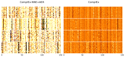
Figure 1: Visualization of real components of entity representations (rows) learned by ComplEx-NNE+AER (left) and ComplEx (right). From top to bottom, entities belong to type reptile, wine_ region, species, and programming_language in turn. Values range from 0 (white) via 0.5 (orange) to 1 (black). Best viewed in color.

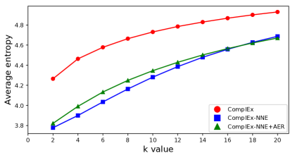
Figure 2: Average entropy over all dimensions of real components of entity representations learned by ComplEx (circles), ComplEx-NNE (squares), and ComplEx-NNE+AER (triangles) as $K$ varies.

Then we investigate the semantic purity of these dimensions. Specifically, we collect the representations of all the entities on DB100K (real components only). For each dimension of these representations, top $K$ percent of entities with the highest activation values on this dimension are picked. We can calculate the entropy of the type distribution of the entities selected. This entropy reflects diversity of entity types, or in other words, semantic purity. If all the $K$ percent of entities have the same type, we will get the lowest entropy of zero (the highest semantic purity). On the contrary, if each of them has a distinct type, we will get the highest entropy (the lowest semantic purity). Figure 2 shows the average entropy over all dimensions of entity representations (real components only) learned by ComplEx, ComplEx-NNE, and ComplEx-NNE+ AER, as $K$ varies. We can see that after imposing the non-negativity constraints, ComplEx-NNE and ComplEx-NNE+AER can learn entity representations with latent dimensions of consistently higher semantic purity. We have conducted the same analyses on imaginary components of entity representations, and observed similar phenomena. The results are given as Appendix A.3.

Figure 3: Visualization of relation representations learned by ComplEx-NNE+AER, with the top 4 relations from the equivalence class, the middle 4 the inversion class, and the bottom 4 others.

4.4 Analysis on Relation Representations

This section further provides a visual inspection of the relation embedding space when the constraints are imposed. To this end, we group relation pairs involved in the DB100K entailment constraints into 3 classes: equivalence, inversion, and others. We choose 2 pairs of relations from each class, and visualize these relation representations learned by ComplEx-NNE+AER in Figure 3, where for each relation we randomly pick 5 dimensions from both its real and imaginary components. By imposing the approximate entailment constraints, these relation representations can encode logical regularities quite well. Pairs of relations from the first class (equivalence) tend to have identical representations $\mathbf{r}_{p}\approx\mathbf{r}_{q}$, those from the second class (inversion) complex conjugate representations $\mathbf{r}_{p}\approx\bar{\mathbf{r}}_{q}$; and the others representations that $\textrm{Re}(\mathbf{r}_{p})\leq\textrm{Re}(\mathbf{r}_{q})$ and $\textrm{Im}(\mathbf{r}_{p})\approx\textrm{Im}(\mathbf{r}_{q})$.

5 Conclusion

This paper investigates the potential of using very simple constraints to improve KG embedding. Two types of constraints have been studied: (i) the non-negativity constraints to learn compact, interpretable entity representations, and (ii) the approximate entailment constraints to further encode logical regularities into relation representations. Such constraints impose prior beliefs upon the structure of the embedding space, and will not significantly increase the space or time complexity. Experimental results on benchmark KGs demonstrate that our method is simple yet surprisingly effective, showing significant and consistent improvements over strong baselines. The constraints indeed improve model interpretability, yielding a substantially increased structuring of the embedding space.

Appendix A Supplemental Material

A.1 Sufficient Condition for Eq. (3)

Given the non-negativity constraints of Eq. (2), a sufficient condition for Eq. (3) to hold, is to further impose the strict entailment constraints of Eq. (4). In fact, given the constraints of Eq. (2) and Eq. (4), we will always have

$$\phi(e_{i},r_{p},e_{j})\;= \langle\textrm{Re}(\mathbf{e}_{i}),\textrm{Re}(\mathbf{r}_{p}),\textrm{Re}(\mathbf{e}_{j})\rangle$$

$$+\langle\textrm{Im}(\mathbf{e}_{i}),\textrm{Re}(\mathbf{r}_{p}),\textrm{Im}(\mathbf{e}_{j})\rangle$$

$$+\langle\textrm{Re}(\mathbf{e}_{i}),\textrm{Im}(\mathbf{r}_{p}),\textrm{Im}(\mathbf{e}_{j})\rangle$$

$$-\langle\textrm{Im}(\mathbf{e}_{i}),\textrm{Im}(\mathbf{r}_{p}),\textrm{Re}(\mathbf{e}_{j})\rangle$$

$$\;\leq \langle\textrm{Re}(\mathbf{e}_{i}),\textrm{Re}(\mathbf{r}_{q}),\textrm{Re}(\mathbf{e}_{j})\rangle$$

$$+\langle\textrm{Im}(\mathbf{e}_{i}),\textrm{Re}(\mathbf{r}_{q}),\textrm{Im}(\mathbf{e}_{j})\rangle$$

$$+\langle\textrm{Re}(\mathbf{e}_{i}),\textrm{Im}(\mathbf{r}_{q}),\textrm{Im}(\mathbf{e}_{j})\rangle$$

$$-\langle\textrm{Im}(\mathbf{e}_{i}),\textrm{Im}(\mathbf{r}_{q}),\textrm{Re}(\mathbf{e}_{j})\rangle$$

$$\;= \phi(e_{i},r_{q},e_{j})$$

for any two entities $e_{i},e_{j}\in\mathcal{E}$, i.e., Eq. (3). Here, the first two terms of the inequality hold because $\textrm{Re}(\mathbf{r}_{p})\leq\textrm{Re}(\mathbf{r}_{q})$, and the last two terms because $\textrm{Im}(\mathbf{r}_{p})=\textrm{Im}(\mathbf{r}_{q})$, given the condition that $\textrm{Re}(\mathbf{e}),$ $\textrm{Im}(\mathbf{e})\geq\mathbf{0}$ for every $e\in\mathcal{E}$.

A.2 Equivalence between Eq. (3.4) and Eq. (3.4)

We first rewrite the constraints of the optimization Eq. (3.4). Specifically, the two constraints

$$\boldsymbol{\alpha}\geq\lambda\big{(}\textrm{Re}(\mathbf{r}_{p})-\textrm{Re}(\mathbf{r}_{q})\big{)},\;\;\boldsymbol{\alpha}\geq\boldsymbol{0}$$

can be rewritten as a single one, i.e.,

$$\boldsymbol{\alpha}\geq\lambda\big{[}\textrm{Re}(\mathbf{r}_{p})-\textrm{Re}(\mathbf{r}_{q})\big{]}_{+},$$

where $[\mathbf{x}]_{+}=\max(\mathbf{0},\mathbf{x})$ with $\max(\cdot,\cdot)$ being an entry-wise operator. Similarly, the two constraints

$$\boldsymbol{\beta}\geq\lambda\big{(}\textrm{Im}(\mathbf{r}_{p})-\textrm{Im}(\mathbf{r}_{q})\big{)}^{2},\;\;\boldsymbol{\beta}\geq\boldsymbol{0}$$

degenerate to a single one, i.e.,

$$\boldsymbol{\beta}\geq\lambda\big{(}\textrm{Im}(\mathbf{r}_{p})-\textrm{Im}(\mathbf{r}_{q})\big{)}^{2}.$$

As the objective function of Eq. (3.4) has to minimize $\boldsymbol{1}^{\top}(\boldsymbol{\alpha}+\boldsymbol{\beta})$ over all possible $\boldsymbol{\alpha},\boldsymbol{\beta}$, an optimal value for this term will be

$$\lambda\boldsymbol{1}^{\top}\big{[}\textrm{Re}(\mathbf{r}_{p})-\textrm{Re}(\mathbf{r}_{q})\big{]}_{+}+\lambda\boldsymbol{1}^{\top}\big{(}\textrm{Im}(\mathbf{r}_{p})-\textrm{Im}(\mathbf{r}_{q})\big{)}^{2}.$$

Plugging this back into the objective function and removing the degenerated constraints, we will obtain the optimization of Eq. (3.4).

A.3 Analyses on Imaginary Components of Entity Representations

We conduct the same analyses on imaginary components of entity representations as those conducted on real ones (§ 4.3). Figure 4 visualizes imaginary components of entity representations learned by ComplEx and ComplEx-NNE+AER, with the optimal configurations determined by link prediction. Figure 5 shows average entropy along imaginary components of entity representations learned by ComplEx, ComplEx-NNE, and ComplEx-NNE +AER.

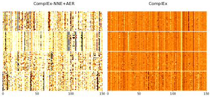
Figure 4: Visualization of imaginary components of entity representations (rows) learned by ComplEx-NNE+AER (left) and ComplEx (right). From top to bottom, entities belong to reptile, wine_ region, species, programming_language in turn. Values range from 0 (white) via 0.5 (orange) to 1 (black). Best viewed in color.

Figure 5: Average entropy over all dimensions of imaginary components of entity representations learned by ComplEx (circles), ComplEx-NNE (squares), and ComplEx-NNE+AER (triangles) as $K$ varies.

A.4 Properties of Equivalence, Inversion, or Ordinary Entailment

For ordinary entailment $r_{p}\rightarrow r_{q}$ (neither equivalence nor inversion), the constraints of Eq. (4) directly suggest

$$\textrm{Re}(\mathbf{r}_{p})\leq\textrm{Re}(\mathbf{r}_{q}),\;\;\textrm{Im}(\mathbf{r}_{p})=\textrm{Im}(\mathbf{r}_{q}).$$

For equivalence $r_{p}\leftrightarrow r_{q}$ ($r_{p}\rightarrow r_{q}$ and $r_{q}\rightarrow r_{p}$), we ought to have

$$\textrm{Re}(\mathbf{r}_{p})\leq\textrm{Re}(\mathbf{r}_{q}),\;\;\textrm{Im}(\mathbf{r}_{p})=\textrm{Im}(\mathbf{r}_{q}),$$

$$\textrm{Re}(\mathbf{r}_{q})\leq\textrm{Re}(\mathbf{r}_{p}),\;\;\textrm{Im}(\mathbf{r}_{q})=\textrm{Im}(\mathbf{r}_{p}),$$

which imply $\mathbf{r}_{p}\!=\!\mathbf{r}_{q}$. Since

$$\phi(e_{i},r_{k},e_{j}) =\textrm{Re}(\langle\mathbf{e}_{i},\mathbf{r}_{k},\bar{\mathbf{e}}_{j}\rangle)$$

$$=\textrm{Re}(\langle\mathbf{e}_{j},\bar{\mathbf{r}}_{k},\bar{\mathbf{e}}_{i}\rangle)$$

$$\triangleq\phi(e_{j},r_{k}^{-1},e_{i})$$

for any $e_{i},e_{j}\in\mathcal{E}$ and $r_{k}\in\mathcal{R}$, we could represent the inverse of relation $r_{k}$ (i.e. $r_{k}^{-1}$) as the conjugate of $\mathbf{r}_{k}$ (i.e. $\bar{\mathbf{r}}_{k}$). Then for inversion $r_{p}\leftrightarrow r_{q}^{-1}$, we ought to have $\mathbf{r}_{p}=\bar{\mathbf{r}}_{q}$.

References

- Bollacker et al. (2008) Kurt Bollacker, Colin Evans, Praveen Paritosh, Tim Sturge, and Jamie Taylor. 2008. Freebase: A collaboratively created graph database for structuring human knowledge. In Proceedings of the 2008 ACM SIGMOD International Conference on Management of Data. pages 1247–1250.
- Bordes et al. (2014) Antoine Bordes, Xavier Glorot, Jason Weston, and Yoshua Bengio. 2014. A semantic matching energy function for learning with multi-relational data. Machine Learning 94(2):233–259.
- Bordes et al. (2013) Antoine Bordes, Nicolas Usunier, Alberto García-Durán, Jason Weston, and Oksana Yakhnenko. 2013. Translating embeddings for modeling multi-relational data. In Advances in Neural Information Processing Systems. pages 2787–2795.
- Bordes et al. (2011) Antoine Bordes, Jason Weston, Ronan Collobert, and Yoshua Bengio. 2011. Learning structured embeddings of knowledge bases. In Proceedings of the 25th AAAI Conference on Artificial Intelligence. pages 301–306.
- Chang et al. (2014) Kai-Wei Chang, Wen-tau Yih, Bishan Yang, and Christopher Meek. 2014. Typed tensor decomposition of knowledge bases for relation extraction. In Proceedings of the 2014 Conference on Empirical Methods in Natural Language Processing. pages 1568–1579.
- Demeester et al. (2016) Thomas Demeester, Tim Rocktäschel, and Sebastian Riedel. 2016. Lifted rule injection for relation embeddings. In Proceedings of the 2016 Conference on Empirical Methods in Natural Language Processing. pages 1389–1399.
- Dettmers et al. (2018) Tim Dettmers, Minervini Pasquale, Stenetorp Pontus, and Sebastian Riedel. 2018. Convolutional 2D knowledge graph embeddings. In Proceedings of the 32nd AAAI Conference on Artificial Intelligence. pages 1811–1818.
- Dong et al. (2014) Xin Dong, Evgeniy Gabrilovich, Geremy Heitz, Wilko Horn, Ni Lao, Kevin Murphy, Thomas Strohmann, Shaohua Sun, and Wei Zhang. 2014. Knowledge vault: A web-scale approach to probabilistic knowledge fusion. In Proceedings of the 20th ACM SIGKDD International Conference on Knowledge Discovery and Data Mining. pages 601–610.
- Duchi et al. (2011) John Duchi, Elad Hazan, and Yoram Singer. 2011. Adaptive subgradient methods for online learning and stochastic optimization. Journal of Machine Learning Research 12(Jul):2121–2159.
- Fyshe et al. (2015) Alona Fyshe, Leila Wehbe, Partha P. Talukdar, Brian Murphy, and Tom M. Mitchell. 2015. A compositional and interpretable semantic space. In Proceedings of the 2015 Conference of the North American Chapter of the Association for Computational Linguistics: Human Language Technologies. pages 32–41.
- Galárraga et al. (2015) Luis Antonio Galárraga, Christina Teflioudi, Katja Hose, and Fabian M. Suchanek. 2015. Fast rule mining in ontological knowledge bases with AMIE+. The VLDB Journal 24(6):707–730.
- Guo et al. (2015) Shu Guo, Quan Wang, Bin Wang, Lihong Wang, and Li Guo. 2015. Semantically smooth knowledge graph embedding. In Proceedings of the 53rd Annual Meeting of the Association for Computational Linguistics and the 7th International Joint Conference on Natural Language Processing. pages 84–94.
- Guo et al. (2016) Shu Guo, Quan Wang, Lihong Wang, Bin Wang, and Li Guo. 2016. Jointly embedding knowledge graphs and logical rules. In Proceedings of the 2016 Conference on Empirical Methods in Natural Language Processing. pages 192–202.
- Guo et al. (2018) Shu Guo, Quan Wang, Lihong Wang, Bin Wang, and Li Guo. 2018. Knowledge graph embedding with iterative guidance from soft rules. In Proceedings of the 32nd AAAI Conference on Artificial Intelligence. pages 4816–4823.
- Hoffmann et al. (2011) Raphael Hoffmann, Congle Zhang, Xiao Ling, Luke Zettlemoyer, and Daniel S. Weld. 2011. Knowledge-based weak supervision for information extraction of overlapping relations. In Proceedings of the 49th Annual Meeting of the Association for Computational Linguistics. pages 541–550.
- Jenatton et al. (2012) Rodolphe Jenatton, Nicolas L. Roux, Antoine Bordes, and Guillaume R. Obozinski. 2012. A latent factor model for highly multi-relational data. In Advances in Neural Information Processing Systems. pages 3167–3175.
- Ji et al. (2015) Guoliang Ji, Shizhu He, Liheng Xu, Kang Liu, and Jun Zhao. 2015. Knowledge graph embedding via dynamic mapping matrix. In Proceedings of the 53rd Annual Meeting of the Association for Computational Linguistics and the 7th International Joint Conference on Natural Language Processing. pages 687–696.
- Kadlec et al. (2017) Rudolf Kadlec, Ondrej Bajgar, and Jan Kleindienst. 2017. Knowledge base completion: Baselines strike back. In Proceedings of the 2nd Workshop on Representation Learning for NLP. pages 69–74.
- Kruszewski et al. (2015) German Kruszewski, Denis Paperno, and Marco Baroni. 2015. Deriving Boolean structures from distributional vectors. Transactions of the Association for Computational Linguistics 3:375–388.
- Lee and Seung (1999) Daniel D. Lee and H. Sebastian Seung. 1999. Learning the parts of objects by non-negative matrix factorization. Nature 401:788–791.
- Lehmann et al. (2015) Jens Lehmann, Robert Isele, Max Jakob, Anja Jentzsch, Dimitris Kontokostas, Pablo N. Mendes, Sebastian Hellmann, Mohamed Morsey, Patrick van Kleef, Sören Auer, et al. 2015. DBpedia: A large-scale, multilingual knowledge base extracted from Wikipedia. Semantic Web Journal 6(2):167–195.
- Lin et al. (2015a) Yankai Lin, Zhiyuan Liu, Huanbo Luan, Maosong Sun, Siwei Rao, and Song Liu. 2015a. Modeling relation paths for representation learning of knowledge bases. In Proceedings of the 2015 Conference on Empirical Methods in Natural Language Processing. pages 705–714.
- Lin et al. (2015b) Yankai Lin, Zhiyuan Liu, Maosong Sun, Yang Liu, and Xuan Zhu. 2015b. Learning entity and relation embeddings for knowledge graph completion. In Proceedings of the 29th AAAI Conference on Artificial Intelligence. pages 2181–2187.
- Liu et al. (2017) Hanxiao Liu, Yuexin Wu, and Yiming Yang. 2017. Analogical inference for multi-relational embeddings. In Proceedings of the 34th International Conference on Machine Learning. pages 2168–2178.
- Luo et al. (2015a) Hongyin Luo, Zhiyuan Liu, Huanbo Luan, and Maosong Sun. 2015a. Online learning of interpretable word embeddings. In Proceedings of the 2015 Conference on Empirical Methods in Natural Language Processing. pages 1687–1692.
- Luo et al. (2015b) Yuanfei Luo, Quan Wang, Bin Wang, and Li Guo. 2015b. Context-dependent knowledge graph embedding. In Proceedings of the 2015 Conference on Empirical Methods in Natural Language Processing. pages 1656–1661.
- Minervini et al. (2017a) Pasquale Minervini, Luca Costabello, Emir Muñoz, Vít Nováček, and Pierre-Yves Vandenbussche. 2017a. Regularizing knowledge graph embeddings via equivalence and inversion axioms. In Joint European Conference on Machine Learning and Knowledge Discovery in Databases. pages 668–683.
- Minervini et al. (2017b) Pasquale Minervini, Thomas Demeester, Tim Rocktäschel, and Sebastian Riedel. 2017b. Adversarial sets for regularising neural link predictors. In Proceedings of the 33rd Conference on Uncertainty in Artificial Intelligence.
- Murphy et al. (2012) Brian Murphy, Partha Talukdar, and Tom Mitchell. 2012. Learning effective and interpretable semantic models using non-negative sparse embedding. In Proceedings of COLING 2012. pages 1933–1950.
- Neelakantan et al. (2015) Arvind Neelakantan, Benjamin Roth, and Andrew McCallum. 2015. Compositional vector space models for knowledge base completion. In Proceedings of the 53rd Annual Meeting of the Association for Computational Linguistics and the 7th International Joint Conference on Natural Language Processing. pages 156–166.
- Nickel et al. (2016a) Maximilian Nickel, Kevin Murphy, Volker Tresp, and Evgeniy Gabrilovich. 2016a. A review of relational machine learning for knowledge graphs. Proceedings of the IEEE 104(1):11–33.
- Nickel et al. (2016b) Maximilian Nickel, Lorenzo Rosasco, and Tomaso Poggio. 2016b. Holographic embeddings of knowledge graphs. In Proceedings of the 30th AAAI Conference on Artificial Intelligence. pages 1955–1961.
- Nickel et al. (2011) Maximilian Nickel, Volker Tresp, and Hans-Peter Kriegel. 2011. A three-way model for collective learning on multi-relational data. In Proceedings of the 28th International Conference on Machine Learning. pages 809–816.
- Rocktäschel et al. (2015) Tim Rocktäschel, Sameer Singh, and Sebastian Riedel. 2015. Injecting logical background knowledge into embeddings for relation extraction. In Proceedings of the 2015 Conference of the North American Chapter of the Association for Computational Linguistics: Human Language Technologies. pages 1119–1129.
- Schlichtkrull et al. (2017) Michael Schlichtkrull, Thomas N. Kipf, Peter Bloem, Rianne van den Berg, Ivan Titov, and Max Welling. 2017. Modeling relational data with graph convolutional networks. arXiv:1703.06103 .
- Shi and Weninger (2017) Baoxu Shi and Tim Weninger. 2017. ProjE: Embedding projection for knowledge graph completion. In Proceedings of the 31st AAAI Conference on Artificial Intelligence. pages 1236–1242.
- Socher et al. (2013) Richard Socher, Danqi Chen, Christopher D. Manning, and Andrew Y. Ng. 2013. Reasoning with neural tensor networks for knowledge base completion. In Advances in Neural Information Processing Systems. pages 926–934.
- Trouillon et al. (2016) Théo Trouillon, Johannes Welbl, Sebastian Riedel, Eric Gaussier, and Guillaume Bouchard. 2016. Complex embeddings for simple link prediction. In Proceedings of the 33rd International Conference on Machine Learning. pages 2071–2080.
- Wang et al. (2017) Quan Wang, Zhendong Mao, Bin Wang, and Li Guo. 2017. Knowledge graph embedding: A survey of approaches and applications. IEEE Transactions on Knowledge and Data Engineering 29(12):2724–2743.
- Wang et al. (2015) Quan Wang, Bin Wang, and Li Guo. 2015. Knowledge base completion using embeddings and rules. In Proceedings of the 24th International Joint Conference on Artificial Intelligence. pages 1859–1865.
- Wang et al. (2014) Zhen Wang, Jianwen Zhang, Jianlin Feng, and Zheng Chen. 2014. Knowledge graph embedding by translating on hyperplanes. In Proceedings of the 28th AAAI Conference on Artificial Intelligence. pages 1112–1119.
- Wasserman-Pritsker et al. (2015) Evgenia Wasserman-Pritsker, William W. Cohen, and Einat Minkov. 2015. Learning to identify the best contexts for knowledge-based WSD. In Proceedings of the 2015 Conference on Empirical Methods in Natural Language Processing. pages 1662–1667.
- Xiao et al. (2016) Han Xiao, Minlie Huang, and Xiaoyan Zhu. 2016. TransG: A generative model for knowledge graph embedding. In Proceedings of the 54th Annual Meeting of the Association for Computational Linguistics. pages 2316–2325.
- Xiao et al. (2017) Han Xiao, Minlie Huang, and Xiaoyan Zhu. 2017. SSP: Semantic space projection for knowledge graph embedding with text descriptions. In Proceedings of the 31st AAAI Conference on Artificial Intelligence. pages 3104–3110.
- Xie et al. (2016a) Ruobing Xie, Zhiyuan Liu, Jia Jia, Huanbo Luan, and Maosong Sun. 2016a. Representation learning of knowledge graphs with entity descriptions. In Proceedings of the 30th AAAI Conference on Artificial Intelligence. pages 2659–2665.
- Xie et al. (2016b) Ruobing Xie, Zhiyuan Liu, and Maosong Sun. 2016b. Representation learning of knowledge graphs with hierarchical types. In Proceedings of the 25th International Joint Conference on Artificial Intelligence. pages 2965–2971.
- Yang and Mitchell (2017) Bishan Yang and Tom Mitchell. 2017. Leveraging knowledge bases in LSTMs for improving machine reading. In Proceedings of the 55th Annual Meeting of the Association for Computational Linguistics. pages 1436–1446.
- Yang et al. (2015) Bishan Yang, Wen-tau Yih, Xiaodong He, Jianfeng Gao, and Li Deng. 2015. Embedding entities and relations for learning and inference in knowledge bases. In Proceedings of the International Conference on Learning Representations.
- Zhong et al. (2015) Huaping Zhong, Jianwen Zhang, Zhen Wang, Hai Wan, and Zheng Chen. 2015. Aligning knowledge and text embeddings by entity descriptions. In Proceedings of the 2015 Conference on Empirical Methods in Natural Language Processing. pages 267–272.