Soft Maximin Estimation for Heterogeneous Data

Abstract

Extracting a common robust signal from data divided into heterogeneous groups can be difficult when each group – in addition to the signal – can contain large, unique variation components. Previously, maximin estimation has been proposed as a robust estimation method in the presence of heterogeneous noise. We propose soft maximin estimation as a computationally attractive alternative aimed at striking a balance between pooled estimation and (hard) maximin estimation.

The soft maximin method provides a range of estimators, controlled by a parameter $\zeta>0$, that interpolates pooled least squares estimation and maximin estimation. By establishing relevant theoretical properties we argue that the soft maximin method is both statistically sensibel and computationally attractive.

We also demonstrate, on real and simulated data, that the soft maximin estimator can offer improvements over both pooled OLS and hard maximin in terms of predictive performance and computational complexity.

A time and memory efficient implementation is provided in the R package SMME available on CRAN.

heterogeneous data, robust estimation, regularization, convex optimization

1 Introduction

We consider the problem of extracting a common signal from heterogeneous data. As heterogeneity is prevalent in large-scale settings our aim is a computationally efficient estimator (solution) with good statistical properties under varying degrees of data heterogeneity.

To make the concept of heterogeneity concrete, consider the linear mixture model with univariate response variables $Y_{1},\ldots,Y_{n}$ generated as

$$Y_{i}=X_{i}^{\top}B_{i}+\varepsilon_{i},\quad i=1,\ldots,n.$$ (1)

Here, $B_{1},\dots,B_{n}$ and the feature vectors $X_{1},\ldots,X_{n}$ are $p$-dimensional random variables and $\varepsilon_{1},\ldots,\varepsilon_{n}$ are univariate noise variables. The feature vectors are observed and assumed i.i.d., and the noise variables are likewise i.i.d. The unobserved variables $B_{1},\dots,B_{n}$ are identically distributed with distribution $F_{B}$ but not necessarily independent, see also Meinshausen and Bühlmann (2015).

Heterogeneity in the model given by (1) is due to the variation in $B_{i}$ as governed by $F_{B}$. Because the $B_{i}$-s can be dependent, model (1) can capture heterogeneity caused by a group structure, that is, when data comes with a natural grouping and $B_{i}$ is constant within groups but vary across groups. Even if data is not grouped, or if the group structure is unknown, it is beneficial to study the setup with a known group structure. In the example below on bike sharing, a group structure is introduced to represent temporal heterogeneity, and Meinshausen and Bühlmann (2015) demonstrate how to construct group structures as part of the inference when no grouping is given.

Our focus is therefore on a setup with $G$ groups and with $B_{i}$ constant within groups. The objective is to learn a single $\beta\in\mathbb{R}^{p}$ that can sensibly be regarded as a common signal of the $B_{i}$-s. Pooling data across groups and computing the OLS estimator may be non-robust, depending on $F_{B}$, and Meinshausen and Bühlmann (2015) introduced maximin estimation as a robust alternative to OLS for heterogeneous data from the model (1). The common signal estimated by maximin estimation is the population quantity called the maximin effect.

While the maximin estimator is robust, it can also be conservative, and we propose soft maximin estimation to strike a good balance between maximin and pooled OLS estimation. The balance is controlled by a tuning parameter $\zeta>0$, with $\zeta\to\infty$ corresponding to maximin estimation. Figure 1 shows the result of applying the soft maximin estimator, for three values of $\zeta$, as well as the pooled OLS estimator to a real data set. It illustrates how predictive performance of the two extreme estimators is interpolated by soft maximin estimation, quantified as cumulative root mean square error over time, see (25).

The specific application illustrated in Figure 1 is described in detail in Section 4.1. The data is on the hourly number of bike shares (see Fanaee-T and Gama (2013)) from two years (2011 and 2012), and the model predicts this number based on weekday, time of the day and the weather. In this application, one year is used for training and the other year is used for validation (prediction). To safeguard against temporal heterogeneity the data is grouped according to the months variable mnth, thus $G=12$. Training on 2011 makes soft maximin with a high value of $\zeta$ too conservative, which leads to poor predictive performance. In this case, pooled OLS or soft maximin with a low $\zeta$ perform best. However, training on 2012 data makes the pooled OLS estimator overfit and soft maximin with a large $\zeta$ has better predictive performance.

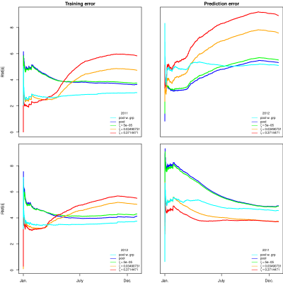
Figure 1: Top: RMSE computed for 2011 training data and 2012 validation data for the soft maximin estimators for 3 values of $\zeta$ (resp. green, orange and red), the pooled OLS estimator (blue) and the pooled OLS estimator using the group variable mnth (cyan). Bottom: RMSE computed for 2012 training data and 2011 validation data using the same methods and coloring.

The paper is organized as follows. The model and estimation framework is outlined in Section 2 and statistical properties of soft maximin estimation are discussed. This section includes theoretical results supporting that soft maximin interpolates maximin and pooled OLS estimation. In Section 3 we propose an algorithm for computing the general soft maximin estimator. The algorithm solves a non-differentiable convex optimization problem, but as opposed to maximin estimation (Meinshausen and Bühlmann, 2015), the problem we solve is separable in the sense of Tseng and Yun (2009). This makes it notably easier to construct efficient algorithms with convergence guarantees. Section 3 also includes theoretical bounds on Lipschitz constants, which can be used to select an efficient step size in our solution algorithm, and a discussion of how our results can be applied efficiently to array tensor smoothing. In Section 4, we present the application to the bike share data and results from a simulation study on array tensor smoothing. The simulation study was inspired by the application to neuronal activity data analyzed in Appendix B. Section 5 summarizes the proposed methodology and its relation to alternative methods. The algorithms are implemented in the R package SMME available from CRAN, see Lund (2021).

2 Soft maximin estimation

Here we present the methodology in a setup with a given group structure and effects $B_{i}$ constant within each group. This in turn implies a finite support for $F_{B}$ and this model is perhaps better understood as a type of linear mixed model as the grouping is available hence no longer part of the inference. In contrast to a traditional mixed model, however, we avoid explicitly modeling fixed and random effects since the aim is not to draw inference about these. Instead we seek to obtain only an estimate of the possible common effects present in the data.

To introduce $G\in\mathbb{N}$ groups for the model (1), suppose given a partition $I_{1},\ldots,I_{G}$ of the index set $\{1,\ldots,n\}$ such that $|I_{g}|=n_{g}$, and $n=\sum_{g}n_{g}$ where for each $g$ and for all $i\in I_{g}$, $B_{i}=B_{g}$ is the effect in group $g$. Thus $F_{B}$ has finite unknown support with cardinality $G$, that is $\mathop{\mathrm{supp}}(F_{B})=\{b_{1},\ldots,b_{G}\}\subset\mathbb{R}^{p}$ with $b_{g}:=B_{g}(\omega)$ the true unknown effect in group $g$.

Using this extra structure we can label the response, covariates and errors according to group. For the $g$th group let $\boldsymbol{Y}_{g}=(Y_{g,1},\ldots,Y_{g,n_{g}})^{\top}$ be the $n_{g}\times 1$ response vector, $\boldsymbol{X}_{g}=(X_{g,1}|\ldots|X_{g,n_{g}})^{\top}$ the $n_{g}\times p$ design matrix, and $\boldsymbol{\varepsilon}_{g}=(\varepsilon_{g,1},\ldots,\varepsilon_{g,n_{g}})^{\top}$ the $n_{g}\times 1$ error vector. The linear model for the $g$th group is then

$$\boldsymbol{Y}_{g}=\boldsymbol{X}_{g}b_{g}+\boldsymbol{\varepsilon}_{g},\quad g\in\{1,\ldots,G\}.$$ (2)

A common signal in this framework is represented by a single $\beta\in\mathbb{R}^{p}$ such that $\boldsymbol{X}_{g}\beta$ is a good and robust approximation of $\boldsymbol{X}_{g}b_{g}$ across all $G$ groups.

To gauge the quality of the approximation we adopt the optimality criterion from Meinshausen and Bühlmann (2015). There the explained variance in group $g$ when using some $\beta\in\mathbb{R}^{p}$ in (2) is defined as

$$V_{b_{g}}(\beta):=2\beta^{\top}\Sigma b_{g}-\beta^{\top}\Sigma\beta.$$ (3)

The optimal approximation across all groups is then the so-called maximin effect defined as a $b^{\ast}\in\mathbb{R}^{p}$ that maximizes the minimum of the explained variances across groups, i.e. $b^{\ast}:=\operatorname*{arg\,max}_{\beta}\min_{g}V_{b_{g}}(\beta)$.

Since $b_{g}$ is unknown, to make this criteria operational, let $\hat{\Sigma}_{g}:=\boldsymbol{X}_{g}^{\top}\boldsymbol{X}_{g}/n_{g}$ denote the empirical Gram matrix in group $g$. By (2) replacing $\Sigma$ with $\hat{\Sigma}_{g}$ in (3) we obtain the empirical explained variance in group $g$

$$\hat{V}_{g}(\beta)\coloneqq\frac{1}{n_{g}}(2\beta^{\top}\boldsymbol{X}_{g}^{\top}\boldsymbol{Y}_{g}-\beta^{\top}\boldsymbol{X}_{g}^{\top}\boldsymbol{X}_{g}\beta).$$ (4)

The maximin effects estimator is obtained by maximizing (the penalized) minimum of (4) or equivalently by minimizing (the penalized) maximin loss function $\beta\mapsto\max_{g}\{-\hat{V}_{g}(\beta)\}$, see (27) in Section 5.

As shown in Meinshausen and Bühlmann (2015) the use of this estimator can lead to more robust estimates for heterogeneous data compared to an estimator that does not take grouping into account i.e. a pooled estimator. The intuition is that the maximin estimator extracts only features that are active with the same sign across groups while setting group specific features to zero. This makes it a more crude estimator compared to one obtained using the full mixed model methodology, however it is in principle also more robust and potentially computationally more attractive. In large scale data settings, where data heterogeneity is typically encountered, the computational aspect of the estimator is crucial. However, since the $\max$-function is non-differentiable and non-separable the maximin problem (27) is not easy to solve.

We address this computational hurdle by replacing the $\max$-function with the following smooth function. For $G\in\mathbb{N}$ and $\zeta\neq 0$ consider the scaled log-sum exponential function

$$\mathrm{lse}_{\zeta}(x)\coloneqq\frac{\log(\sum_{j}e^{\zeta x_{j}})}{\zeta},\quad x\in\mathbb{R}^{G}.$$ (5)

Clearly $\mathrm{lse}_{\zeta}$ is differentiable and as we show in Section 3 it has additional properties that makes it well suited for optimization purposes. First, the basic properties stated next are easily verified (see the appendix) and highlight why (5) is a sensible choice as an approximation of the $\max$-function.

Lemma 1.

Let $G\in\mathbb{N}$ and $x\in\mathbb{R}^{G}$.

1. For $\zeta>0$ it holds that

   $$\max\{x_{1},\ldots,x_{G}\}\leq\mathrm{lse}_{\zeta}(x)\leq\frac{\log(G)}{\zeta}+\max\{x_{1},\ldots,x_{G}\},$$ (6)

   and in particular $\mathrm{lse}_{\zeta}(x)\searrow\max_{g}\{x_{g}\}$ as $\zeta\to\infty$.

2. For $\zeta\to 0$ it holds that

   $$\mathrm{lse}_{\zeta}(x)=\frac{1}{G}\sum_{j=1}^{G}x_{j}+\frac{\log(G)}{\zeta}+o(1).$$

We define the soft maximin loss function, by

$$s_{\zeta}(\beta)\coloneqq\mathrm{lse}_{\zeta}(-\hat{V}(\beta)),\quad\beta\in\mathbb{R}^{p},\quad\zeta>0,$$

where $\hat{V}(\beta):=(\hat{V}_{1}(\beta),\ldots,\hat{V}_{G}(\beta))^{\top}$. For $\kappa>0$ and $\zeta>0$, the soft maximin estimator can now be defined by

$$\hat{\beta}^{\kappa}_{smm}:=\arg\min_{\beta}\mathrm{lse}_{\zeta}(-\hat{V}(\beta))\quad\text{s.t.}\quad\|\beta\|_{1}\leq\kappa.$$ (7)

Using Lemma 1, it is possible to quantify the impact of the parameter $\zeta$ on the performance of the soft maximin estimator (7). The following result gives a bound on the maximum negative explained variance of the soft maximin estimator, using that of the theoretical maximin effect $b^{\ast}$.

Proposition 1.

Let $D=\max_{g}\|\hat{\Sigma}_{g}-\Sigma\|_{\infty}$ and $\delta=\max_{g}\|\boldsymbol{X}_{g}^{\top}\boldsymbol{\varepsilon}_{g}/n_{g}\|_{\infty}$. For fixed $\zeta>0$ and $\kappa>0$, if $\kappa\geq\max_{g}\|b_{g}\|_{1}$,

$$\max_{g}\{-V_{b_{g}}(\hat{\beta}_{smm}^{\kappa})\}\leq\max_{g}\{-V_{b_{g}}(b^{\ast})\}+6D\kappa^{2}+4\kappa\delta+\frac{\log(G)}{\zeta},$$

where $b^{\ast}$ is the maximin effect. In particular

$$\|\hat{\beta}_{smm}^{\kappa}-b^{\ast}\|_{\Sigma}\leq 6\kappa^{2}D+4\kappa\delta+\frac{\log(G)}{\zeta}.$$

Proposition 1 is shown by combining Lemma 1 and results in Meinshausen and Bühlmann (2015), see the appendix. In particular, the performance loss incurred when using the soft maximin estimator is bounded by the same quantity as that of the maximin estimator plus the soft maximum approximation bias $\log(G)/\zeta$ from Lemma 1. Thus the soft maximin estimator enjoys theoretical properties similar to those of the (hard) maximin estimator, when controlling for the parameter $\zeta$. In particular, for $D=0$ (e.g. for a fixed design) and a fixed number of groups, if $n_{g}\to\infty$ for all $g$, the soft maximin estimator only retains the approximation bias.

Proposition 1 establishes a connection between the soft maximin performance and the maximin effect and shows that for $\zeta\uparrow\infty$ we indeed obtain the maximin estimator performance. However, it also highlights that for $\zeta\downarrow 0$ the performance of the soft maximin estimator can stray arbitrarily far away from that of the maximin estimator. To shed light on this note that by Lemma 1, for small $\zeta>0$,

$$s_{\zeta}(\beta)\approx\frac{1}{G}\sum_{j=1}^{G}-\hat{V}_{j}(\beta)+\frac{\log(G)}{\zeta}\propto\frac{1}{n}\sum_{j=1}^{G}\sum_{i=1}^{n_{j}}\frac{n}{Gn_{j}}((X_{j}\beta)_{i}-Y_{j,i})^{2}$$

and (7) effectively becomes a penalized weighted least squares (PWLS) problem over all $n$ observations. Thus solving (7) for a small $\zeta\geq 0$ approximately yields the pooled PWLS estimator with weights amplifying observations from smaller than average groups. With the same number of observations in each group, the soft maximin estimator in turn interpolates the pooled PLS estimator and the maximin estimator.

In this sense $\zeta$ reflects the heterogeneity in the data. If there is little heterogeneity a low or even zero $\zeta$ might work well corresponding to grouping not being relevant. However, for heterogeneous data a low $\zeta$ might lead to predictions that are worse than the zero prediction, whereas a high $\zeta$ can still work well.

To illustrate the interpolation, consider a small data example with data generated according to (2) with $G=20$ groups, $n_{g}=400$ observations in each group, and a two-dimensional parameter space. For fixed effects $\{b_{1},\ldots,b_{20}\}\subset\ \mathbb{R}^{2}$ we sample $\boldsymbol{X}_{g}$ and $\boldsymbol{\varepsilon}_{g}$, $M=10$ times for each $g$ resulting in 10 different data sets. For each of these ten small data sets we can compute the unpenalized softmaximin estimate (i.e. $\kappa=\infty$ in (7)) for a sequence of $\zeta$ values as well as the corresponding maximin estimate (i.e. $\lambda=0$ in (27)) using base functionality in R.

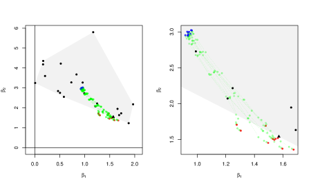
Figure 2: Left: Convex hull (grey shaded area) of $\mathop{\mathrm{supp}}F_{B}$ (black points). Theoretical maximin effect $b^{\ast}$ ($\blacktriangle$), maximin estimates (red points), soft maximin estimates (green points) for various $\zeta$, and population LS estimates (blue points). Right: Close up.

Figure 2 displays the interpolation paths of the softmaximin estimator connecting the population LS estimates and the maximin estimates. Note that all maximin type estimates are clustered around the theoretical maxmin effect indicated with a $\blacktriangle$ on the edge of the convex hull of $\{b_{1},\ldots,b_{20}\}$ while the pooled estimates are well inside the convex hull.

We note that very recently another regression method, anchor regression, was proposed in Rothenhäusler et al. (2021) to handle data heterogeneity in situations where the response distribution can shift yielding a difference between the training data distribution and test data distribution. If this heterogeneity can be encoded or generated by a known anchor variable their method can lead to improved and particularly more stable prediction performance. Especially by controlling for an anchor parameter $\gamma>0$, this method interpolates three different regression methods where $\gamma=1$ yields OLS regression and $\gamma=\infty$ an instrumental variabel regression.

In some sense the anchor plays the role of the grouping structure $I_{1},\ldots,I_{G}$ used in the definition of the softmaximin estimator. However we note that in a general setup with unknown groups, given certain structural assumptions, we may construct index sets $I_{1},\ldots,I_{G}$ e.g. as in the example above or by random sampling. Theoretical guarantees in this case are given in Meinshausen and Bühlmann (2015) for the maximin estimator and similarly to Proposition 1 should extend to the soft maximin estimator.

In addition to mathematical complexity, this adds a layer of substantial computational complexity to the inference procedure since the number of groups $G$ is then a hyperparameter that needs to be inferred e.g. by cross validation. Thus this clustering layer only amplifies the importance of an efficiently computable base estimator.

3 Computational properties

Here we shall consider a general estimation setup where the empirical explained variance $-\hat{V}_{g}$ from (4) is replaced by a general convex group divergence function, $h_{g}:\mathbb{R}^{p}\to\mathbb{R}$. Particularly, in parallel to the Bregman divergence let $\psi:\mathbb{R}^{n}\to\mathbb{R}$ be a convex function, and define

$$D_{\psi}(x,y):=\psi(x)-\nabla\psi(y)^{\top}x,\quad x,y\in\mathbb{R}^{n}.$$

The group divergence function can then be defined by

$$h_{g}(\beta):=D_{\psi}(\eta_{g}(\beta),Y_{g}),\quad\beta\in\mathbb{R}^{p},$$

where $\eta_{g}(\beta)=\boldsymbol{X}_{g}\beta$ is the linear predictor in group $g$. Note that as $\psi$ is convex it follows that $D_{\psi}$, like the Bregman divergence, is convex in its first argument and in particular $h_{g}$ is convex. However, unlike the Bregman divergence $D_{\psi}$ is not non-negative.

A general soft maximin loss function $l_{\zeta}:\mathbb{R}^{p}\to\mathbb{R}$, is now given by

$$l_{\zeta}(\beta):=\mathrm{lse}_{\zeta}\circ h(\beta)=\frac{\log(\sum_{j=1}^{G}e^{\zeta h_{j}(\beta)})}{\zeta},\quad\zeta>0,$$

and our aim is to solve the general soft maximin problem formulated as

$$\min_{\beta\in\mathbb{R}^{p}}l_{\zeta}(\beta)+\lambda J(\beta),\quad\lambda\geq 0.$$ (8)

Here $J$ is a proper convex penalty function and $\lambda$ is the penalty parameter.

Choosing $\psi$ as the square norm yields the negative empirical explained variance $-\hat{V}_{g}$ as group divergence i.e. $h=-\hat{V}$. If $J=\|\cdot\|_{1}$, both loss and penalty are convex in this case, and (8) is equivalent to the (constrained) soft maximin problem (7) by strong Lagrangian duality. Hence in this case the solution to (8) is exactly the soft maximin estimator.

We note that for a different choice of $\psi$ we would obtain an entirely new estimator potentially with properties very different from those of the soft maximin estimator. An immediate Mahalanobis type generalization would arise if we let $\psi$ be given as a weighted square norm.

Solving (8) in a large scale setting requires an efficient optimization algorithm for non-differentiable problems. In contrast to the hard maximin problem, (8) is, in addition to convex and non-differentiable, a (partially) differentiable and separable problem (see Tseng and Yun (2009)). This means that a range of efficient algorithm will solve (8) e.g. first order operator splitting algorithms like ADMM or a second order algorithm like coordinate descent. Here we are going to consider modified versions of the proximal gradient algorithm.

3.1 Solution algorithm

The proximal gradient algorithm fundamentally works by iteratively applying the proximal operator

$$\mathrm{prox}_{\Delta J}(\beta)=\operatorname*{arg\,min}_{\gamma\in\mathbb{R}^{p}}\Big{\{}\frac{1}{2\Delta}\|\gamma-\beta\|_{2}^{2}+J(\gamma)\Big{\}},\quad\Delta>0$$ (9)

to gradient based proposal steps. For a loss function with a Lipschitz continuous gradient with constant $L$, such an algorithm is guaranteed to converge to the solution as long as $\Delta\in(0,2/L)$, hence making it attractive to obtain the smallest possible Lipschitz constant $L$.

With known $L$ and fixed $\Delta\in(0,2/L)$ a proximal gradient algorithm essentially consists of the following steps:

1. evaluate the gradient of the loss

2. evaluate the proximal operator $\mathrm{prox}_{\Delta J}$

3. evaluate the loss function and penalty function.

The computational complexity in steps 1 and 3 is dominated by matrix-vector products, (see e.g. (4) for the soft maximin problem). The complexity in step 2 is determined by $J$. As noted in Beck and Teboulle (2009) when $J$ is separable (e.g. the $\ell_{1}$-norm) $\mathrm{prox}_{\Delta J}$ can be computed analytically or at low cost.

If $L$ is not known (or if $\Delta\geq 2/L$ for a known, but perhaps conservative, $L$) we cannot guarantee convergence with a fixed choice of $\Delta$, but adding a backtracking step will ensure convergence of the iterates. This extra step will increase the per-step computational cost of the algorithm.

When the gradient is not globally Lipschitz, it is no longer guaranteed that iterating steps 1-3 will yield a solution to (8) for any fixed $\Delta$. However, we verify (Proposition 3) that the following non-monotone proximal gradient (NPG) algorithm, see Wright et al. (2009) and Chen et al. (2016), will converge to a solution of (8) under some regularity conditions.

Algorithm 1 NPG minimizing $F=f+\lambda J$

0:  $\beta^{0}$, $L_{\max}\geq L_{\min}>0$, $\tau>1$, $c>0$, $M\in\mathbb{N}$.

1:  for $k=0$ to $K\in\mathbb{N}$ do

2:      choose $L_{k}\in[L_{\min},L_{\max}]$

3:      solve $\beta=\mathrm{prox}_{\lambda J/L_{k}}(\beta^{(k)}-\frac{1}{L_{k}}\nabla f(\beta^{(k)}))$

4:     if  $F(\beta)\leq\max_{[k-M]_{+}\leq i\leq k}F(\beta^{(i)})-c/2\|\beta-\beta^{(k)}\|^{2}$ then

5:        $\beta^{(k+1)}=\beta$

6:     else

7:        $L_{k}=\tau L_{k}$ and go to 3

8:     end if

9:  end for

In particular, we show that while $l_{\zeta}$ does not have a Lipschitz continuous gradient in general, convergence of the NPG algorithm is still guaranteed under general conditions on the group functions $h_{1},\ldots,h_{G}$. Furthermore, in the special case where $h_{g}=-\hat{V}_{g}$ with all groups sharing the same design we show that $l_{\zeta}$ has a globally Lipschitz continuous gradient, and we derive a Lipschitz constant.

The first result states that $l_{\zeta}$ inherits strong convexity from any individual group divergence function $h_{g}$ given that all $h_{1},\ldots,h_{G}$ are convex and twice continuously differentiable. The proof is given in the appendix.

Proposition 2.

For $g\in\{1,\ldots,G\}$ assume $h_{g}$ is twice continuously differentiable and let $w_{g,\zeta}(\beta):=e^{\zeta h_{g}(\beta)-\zeta l_{\zeta}(\beta)},\beta\in\mathbb{R}^{p}$. Then $(w_{j,\zeta}(\beta))_{j}$ are convex weights and

$$\nabla l_{\zeta}(\beta) = \sum_{j=1}^{G}w_{j,\zeta}(\beta)\nabla h_{j}(\beta)$$ (10)

$$\nabla^{2}l_{\zeta}(\beta) = \sum_{i=1}^{G}\sum_{j=i+1}^{G}w_{i,\zeta}(\beta)w_{j,\zeta}(\beta)(\nabla h_{i}(\beta)-\nabla h_{j}(\beta))(\nabla h_{i}(\beta)-\nabla h_{j}(\beta))^{\top}$$

$$+\sum_{j=1}^{G}w_{j,\zeta}(\beta)\nabla^{2}h_{j}(\beta).$$ (11)

Furthermore if $h_{1},\ldots,h_{G}$ are convex with at least one $h_{g}$ strongly convex, then $l_{\zeta}$ and $e^{\zeta l_{\zeta}}$ are strongly convex.

Proposition 2 applies to the soft maximin loss with $h_{g}=-\hat{V}_{g}$. In this case $\nabla^{2}h_{g}=2\boldsymbol{X}^{\top}_{g}\boldsymbol{X}_{g}/n_{g}$, and $h_{g}$ is strongly convex if and only if $\boldsymbol{X}_{g}$ has rank $p$. Proposition 2 implies that if one of the matrices $\boldsymbol{X}_{g}$ has rank $p$, $l_{\zeta}$ is strongly convex. However, we also see from Proposition 2 that $\nabla^{2}l_{\zeta}(\beta)$ is not globally bounded in general. Consider the soft maximin loss, for instance, with $G=2$, $p=n_{1}=n_{2}=2$ and

$$\boldsymbol{X}_{1}=\left(\begin{array}[]{cc}1&0\\ 0&1\end{array}\right)\quad\textrm{and}\quad\boldsymbol{X}_{2}=\left(\begin{array}[]{cc}0&0\\ \sqrt{2}&0\end{array}\right).$$ (16)

Take also $y_{1}=y_{2}=0$. When $\beta_{1}=\beta_{2}=r\in\mathbb{R}$ it holds that $h_{1}(\beta)=h_{2}(\beta)=r^{2}$ and thus $w_{1,\zeta}=w_{2,\zeta}=1/2$ for any $\zeta$, while

$$(\nabla h_{1}(\beta)-\nabla h_{2}(\beta))(\nabla h_{1}(\beta)-\nabla h_{2}(\beta))^{\top}$$

$$=\left(\begin{array}[]{cc}\beta_{1}^{2}&-\beta_{1}\beta_{2}\\ -\beta_{1}\beta_{2}&\beta_{2}^{2}\end{array}\right) =\left(\begin{array}[]{cc}r^{2}&-r^{2}\\ -r^{2}&r^{2}\end{array}\right)$$

is unbounded.

The following result shows, on the other hand, that for soft maximin estimation with identical $\boldsymbol{X}_{g}$-matrices across the groups, $\nabla l_{\zeta}$ is, in fact, Lipschitz continuous. The proof is in the appendix.

Corollary 1.

For each $g\in\{1,\ldots,G\}$ let $\boldsymbol{X}_{g}=\boldsymbol{X}$ be a $m\times p$ matrix, $\boldsymbol{Y}_{g}$ a $m\times 1$ vector and the group divergence given by

$$h_{g}(\beta)=\frac{1}{m}(2\beta^{\top}\boldsymbol{X}^{\top}\boldsymbol{Y}_{g}-\beta^{\top}\boldsymbol{X}^{\top}\boldsymbol{X}\beta).$$

Then $\nabla l_{\zeta}$ has Lipschitz constant $L$ bounded by

$$\frac{4}{m^{2}}\max_{i,j}\|\boldsymbol{X}^{\top}(\boldsymbol{Y}_{i}-\boldsymbol{Y}_{j})\|^{2}+\frac{2\vvvert\boldsymbol{X}^{\top}\boldsymbol{X}\vvvert}{m}\leq\frac{4\vvvert\boldsymbol{X}^{\top}\boldsymbol{X}\vvvert}{m^{2}}\Big{(}\max_{i,j}\|\boldsymbol{Y}_{i}-\boldsymbol{Y}_{j}\|^{2}+\frac{m}{2}\Big{)},$$ (17)

with $\vvvert\cdot\vvvert$ the matrix norm induced by the 2-norm $\|\cdot\|$.

By Corollary 1 if we have identical designs across groups we can obtain the soft maximin estimator by applying the fast proximal gradient algorithm from Beck and Teboulle (2009) to the optimization problem (8). Furthermore in this setting the corollary gives an explicit expression for the Lipschitz constant that will yield an efficient step size $\Delta$ for the solution algorithm.

Finally, in the general setup the following proposition shows that Algorithm 1, which does not rely on a global Lipschitz property (Chen et al. (2016)), solves the problem (8) given the assumptions in Proposition 2. The proof of the proposition is given in the appendix.

Proposition 3.

Assume $h_{1},\ldots,h_{G}$ satisfy the assumptions in Proposition 2. Let $(\beta^{(k)})_{k}$ be a sequence of iterates obtained by applying the NPG algorithm to (8). Then $\beta^{(k)}\to\beta^{\ast}$ where $\beta^{\ast}$ is a critical point of $l_{\zeta}+\lambda J$.

In summary given a strongly convex group divergence function, e.g. satisfied in the soft maximin setup when one $\boldsymbol{X}_{g}$ has full rank, we can always solve the general problem (8) using a proximal gradient based algorithm.

3.2 Array tensor smoothing

We shall here briefly discuss an important special case, array tensor smoothing, where the design is fixed and identical across groups and the objective is to extract a common signal understood as a smooth function over a possibly multi-dimensional domain. Typically the scale of the data in this setting, will prevent the (hard) maximin estimator from being applicable.

By array data we mean data with a geometry such that it is most naturally organized in a multidimensional array, as opposed to an unstructured vector. Canonical examples are images, movies, etc.. To formalize this data setting and model consider a regular grid in $\mathbb{R}^{d}$ i.e. a $d$-dimensional lattice

$$\mathcal{Z}_{1}\times\mathcal{Z}_{2}\times\ldots\times\mathcal{Z}_{d}$$ (18)

where $\mathcal{Z}_{j}=\{z_{j,1},\ldots,z_{j,m_{j}}\}\subset\mathbb{R}$ with $m_{j}\in\mathbb{N},j\in\{1,\ldots,d\}$. Let $m:=\prod_{j=1}^{d}m_{j}$. If for each group $g$ data $y_{g,1},\ldots,y_{g,m}$ is sampled across all points in (18) it may be organized in a fully populated $d$-dimensional $m_{1}\times\cdots\times m_{d}$-array

$$\textbf{Y}_{g}=(y_{g,i_{1},\ldots,i_{d}})_{i_{1},\ldots,i_{d}},\quad i_{j}=1,\ldots,m_{j},\ j=1,\ldots,d.$$ (19)

For this reason we refer to this type of data as array data.

Preserving the array structure when formulating a multivariate smoothing model in this data setting leads to the array model equation

$${Y}_{g,i_{1},\ldots,i_{d}}=f_{g}(z_{1,i_{1}},\ldots,z_{d,i_{d}})+\epsilon_{g,i_{1},\ldots,i_{d}},\quad z_{j,i_{j}}\in\mathcal{Z}_{j},$$ (20)

for each $g\in\{1,\ldots,G\}$, where $f_{g}$ is a smooth group signal and $\epsilon_{g,i_{1},\ldots,i_{d}}$ an appropriate error term.

To obtain a linear array model from (20) we parameterize $f_{g}$ using a basis expansion. A particularly convenient way of representing a multivariate function, is to use the tensor product construction to specify multivariate basis functions in terms of (tensor) products of families of univariate basis functions $((\varphi_{j,k})_{k=1}^{\infty})_{j=1}^{d}$. That is with $\varphi_{j,k}:\mathbb{R}\to\mathbb{R}$ the $k$th basis function in the $j$th dimension ($k$th $j$-marginal basis function), we can represent the smooth signal as

$$f_{g}(z_{1},\ldots,z_{d})=\sum_{k_{1},\ldots,k_{d}}\Theta_{g,k_{1},\ldots,k_{d}}\prod_{j=1}^{d}\varphi_{j,k_{j}}(z_{j}),\quad z_{j}\in\mathbb{R},$$ (21)

where $(\Theta_{g,k_{1},\ldots,k_{d}})_{k_{1},\ldots,k_{d}}$ are basis coefficients.

Now, in order to implement this representation for the model (20) we need to determine the number of basis functions to use in the $j$the dimension, $p_{j}\in\mathbb{N}$, to obtain an (finite) approximation of $f_{g}$. For tensor product basis functions it is customary to choose $p_{j}$ as a function of the cardinality of $\mathcal{Z}_{j}$ e.g. $p_{j}=[m_{j}/5]$ (see Currie et al. (2006)).

With $p_{j}\in\mathbb{N}$ fixed for each $j\in\{1,\ldots,d\}$ we obtain the model (20) as a linear array model in the following way. For each $j\in\{1,\ldots,d\}$ define a $m_{j}\times p_{j}$ matrix $\Phi_{j}=(\varphi_{j,k}(z_{j,i}))_{i,k}$ containing the values of the $p_{j}$ basis functions evaluated at the $m_{j}$ points in $\mathcal{Z}_{j}$. We call $\Phi_{j}$ a marginal design matrix. Also define a $p_{1}\times\cdots\times p_{d}$-array $\boldsymbol{\Theta}_{g}=(\Theta_{g,j_{1},\ldots,j_{d}})_{j_{1}=1,\ldots,j_{d}=1}^{p_{1},\ldots,p_{d}}$ containing the corresponding basis coefficients.

It then follows directly from the identity (21) that the tensor (Kronecker) product of these marginal design matrices,

$$\Phi=\Phi_{d}\otimes\cdots\otimes\Phi_{2}\otimes\Phi_{1},$$ (22)

is the design matrix for the linear model version of (20). This means that we can in principle implement (20) as a standard linear model using $\Phi$. However from a computational complexity perspective that is suboptimal and potentially not feasible in large scale data settings as $\Phi$ grows as $\prod p_{j}\prod m_{j}$.

Instead, we can exploit the array tensor structure of the problem and only rely on the much smaller marginal matrices. As shown in Currie et al. (2006) any linear model with array structured data (19) and tensor structured design (22) can be formulated as a linear array model and fitted using so-called array arithmetic. The key computation is the rotated $H$-transform $\rho$, (see Currie et al. (2006) for details), that allows us to write the model (20) as a linear array model

$$\textbf{Y}_{g}=\rho(\Phi_{d},\rho(\Phi_{d-1},\ldots,\rho(\Phi_{1},\boldsymbol{\Theta}_{g})))+\boldsymbol{\epsilon}_{g},$$ (23)

where $\boldsymbol{\epsilon}_{g}$ is a $m_{1}\times\cdots\times m_{d}$ array containing the error terms.

As indicated by (23), using $\rho$ the design matrix-parameter vector products, needed in steps 1 and 3 above, are computed without having access to the (very large) matrix $\Phi$. In addition the computation has lower complexity than the corresponding matrix-vector product (De Boor (1979), Buis and Dyksen (1996)).

Finally, the tensor structure in (22) makes the constant $L$ in Corollary 1 easy to compute, see (30) in Lund et al. (2017). The implication is that we can run the proximal gradient algorithm without performing any backtracking.

Following Lund et al. (2017) we have implemented both the fast proximal algorithm as well as the NPG algorithm 1 in a way that exploits the array-tensor structure described above. Implementations are provided for 1D, 2D, and 3D array data in the R package SMME, Lund (2021) along with the implementation for general unstructured data.

4 Numerical experiments

To demonstrate the properties of the soft maximin estimator we present two data examples. The first example is a real data set, also analyzed in Rothenhäusler et al. (2021), with seemingly a high signal to noise ratio and moderate data heterogeneity. We use this data set to highlight the interpolation property inherent in the soft maximin methodology.

In the second example we use a simulated large-scale data set with low signal to noise ratio and strong heterogeneity to benchmark our methodology. We compare the run time and prediction accuracy of the soft maximin estimator to that of the pooled OLS estimator and the maximin aggregation method, see Bühlmann and Meinshausen (2016). This simulation based example is inspired by a large scale neuronal data set analyzed in Appendix B.

4.1 Washington DC bike sharing data

The data used to produce the results in Figure 1 are described in Fanaee-T and Gama (2013). The data set contains two years (2011 and 2012) of data (variable cnt see Figure 3) from a bike sharing scheme in Washington DC along with auxiliary data presumably relevant for bike usage e.g. weather. We model the hourly number of bike shares from the data set shown in Figure 3. Specifically the square root of the number of bike events (cnt) is modelled as a smooth function of hour of day (hr with values 0 to 23), smooth function of day of week (weekday with values 0 to 6) and the weather situation (weathersit with levels 1,2,3). The model equation for observation $i$ can be written as

$$\sqrt{\texttt{cnt}_{i}}=\sum_{j=1}^{10}\alpha_{j}\phi_{j}(\texttt{hr}_{i})+\sum_{j=1}^{5}\beta_{j}\phi_{j}(\texttt{weekday}_{i})+\sum_{j=1}^{3}\gamma_{j}1_{j}(\texttt{weathersit}_{i})+\epsilon_{i}$$ (24)

where $\phi$ are cubic basis spline functions.

Figure 3: Hourly number of bike shares in Washington DC 2011 and 2012.

Note the raw data do not contain any hours with zero counts. However as there are 165 hours unaccounted for in the data set, we suspect these are hours with zero counts (e.g. during hurricane Sandy in Oct. 2012) and impute this data for simplicity. This imputation has no effect on the analysis. Also there are three observations that have weathersit = 4. To have all weathersit levels present for the relevant test and train split we change the level of these observations to 3. Again this change has no effect relative to leaving out the observations entirely.

The data do not a priori have a grouping structure that explains the heterogeneity. However, a safeguard against temporal heterogeneity may be obtained by using the variable mnth to group the data in months. Using this grouping, to show the effect of the temporal heterogeneity, we perform a simple experiment where we i) fit the model on 2011 data and predict on 2012 data and ii) fit the model on 2012 data and predict on 2011 data.

We fit the model (24) to data using the unpenalized soft maximin estimator ($\lambda=0$ in (8)) and the pooled OLS estimator. We also fit an extension of (24) that includes a smooth function of the grouping variable mnth using OLS. This model potentially controls for the heterogeneity and might have superior performance. Note the aim of the analysis is not to obtain the model with best predictive performance but rather to highlight how maximin type estimators can safeguard against heterogeneity. In settings where the source of structured variation is more opaque and cannot be taken into account easily in the model this idea may still work.

Figure 1 shows the cumulative root mean squared error

$$\text{RMSE}_{\zeta}(t)=\sqrt{\frac{1}{t}\sum_{i=1}^{t}(y_{i}-\hat{y}_{i,\zeta})^{2}}$$ (25)

on both training data and test data for the model fit for respectively i) and ii). Here $y=\sqrt{\texttt{cnt}}$ and $\hat{y}_{\zeta}$, the fitted values for resp. pooling ($\zeta=0$) and soft maximin ($\zeta>0$), are chronologically ordered.

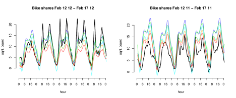
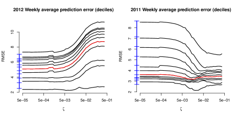
Figure 4: Top: Predictions for 2012 when training on 2011 (left) and for 2011 when training on 2012 (right), for the soft maximin estimator with $\zeta\in\{0.0001,0.01,1\}$ (resp. green, orange and red), the pooled OLS estimator (blue and cyan) and $\sqrt{\texttt{cnt}}$ (black). Bottom: Deciles of weekly averaged prediction error on 2012 data for 2011 training data (left) and on 2011 data for 2012 training data (right) for soft maximin estimation as a function of $\zeta$. Blue part of the $y$-axis shows deciles of the pooled estimator. Red curve indicates the median.

The findings in Figure 1 are in line with Figure 4 that shows the predictions (out of sample) for 5 consecutive days for experiments i) and ii). In the left panel we observe that the high $\zeta$ soft maximin (red) underfits the 2012 data while the low $\zeta$ soft maximin like pooling predicts well. Conversely in the right panel the low $\zeta$ and pooling overfits the high levels observed in some parts of the 2012 data and the result is worse predictions on the 2011 data.

The bottom panel in Figure 4 shows the deciles of RMSEs for the test set (2012 resp. 2011) averaged for each week as a function of $\zeta$. Training on 2011 data and testing on 2012 data shows weekly averaged prediction error of the pooling estimator to have lower median and more narrow support than soft maximin estimators. Conversely training on 2012 data and testing on 2011 a strictly positive $\zeta$ yields more stable predictions and also a lower median. Note the Figure resembles that of Figure 5 in Rothenhäusler et al. (2021).

In Appendix C we fit alternative models that include temperature and humidity. The results are similar to those presented above. We also fit a model where we use weathersit as grouping. For this grouping the soft maximin estimators still appear attractive but the picture is less clear.

Also in the appendix a cross validation scheme is used to tune $\zeta$ for experiment i) and ii). The results are in line with the findings in figures 1 and 4 and suggest that hard maximin is not optimal in neither i) nor ii). For i) pooling ( $\zeta=0$) works best and for ii) a $\zeta$ around 0.03 results in the lowest prediction error. Fitting a spectrum of estimators can be advantageous compared to fitting either of the extreme estimators, pooling respectively maximin, in the given context.

4.2 Benchmark on simulated array data

To benchmark the soft maximin method against existing alternatives we set up a prediction experiment for the model described in Section 3.2 on a simulated data set. In appendix B we carry out the same experiment on a real large scale neuroscientific data set. The experiment is structured like $K$-fold cross validation aimed at discerning the optimal choice of hyperparameters $\zeta$ and $\lambda$ in a grid search.

To evaluate the performance of the soft maximin estimator as a function of the parameter $\zeta$ we train the model for $\zeta\in\{2,100,200\}$. We also compute the pooled estimator corresponding to $\zeta=0$ and the maximin aggregation (magging) estimator from Bühlmann and Meinshausen (2016). In general magging is approximately (hard) maximin estimation and should therefore correspond to $\zeta=\infty$.

This in turn entails solving five different $\ell_{1}$-penalized estimation problems:

• To obtain the three soft maximin estimators we need to solve the problem (8) with $\ell_{1}$-norm penalty for each $\zeta\in\{2,100,200\}$. To do this we use the R package SMME, Lund (2021).

• With identical (fixed) design across groups, we obtain the (penalized) pooled estimator as (penalized) regression of the empirical average across groups on the fixed design. We use the R package glamlasso, Lund (2018) to solve the resulting lasso problem.

• For the magging estimator we have to solve a lasso problem for each group, given $\lambda$ and the design. We use the R package glamlasso, Lund (2018) to obtain the individual group fits. These fits are then maximin aggregated (magging) across groups by solving a quadratic optimization problem as proposed in Bühlmann and Meinshausen (2016).

All computations are carried out on a Macbook Pro with a 2.8 GHz Intel core i7 processor and 16 GB of 1600 MHz DDR3 memory.

4.2.1 Simulated array data

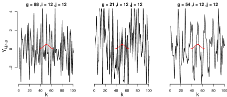
Figure 5: Temporal plot of the simulated data (black) for three different groups and the underlying common Gaussian signal (red).

We simulate data with three components: i) a common Gaussian signal of interest $\phi(x,y,t)=200\phi_{12.5,4}(x)\phi_{12.5,4}(y)\phi_{50,25}(t)$ ($\phi_{\mu,\sigma^{2}}$ is the density for the $\mathcal{N}(\mu,\sigma^{2})$ distribution) superimposed with ii) periodic group specific signals with randomly varying frequency and phase and iii) additive white noise. Specifically for each $g\in\{1,\ldots,G\}$ the 3-dimensional data array was simulated according to

$$Y_{g,i,j,k} =\phi(x_{i},y_{j},t_{k})+5\sum_{j\in J_{g}}\varphi_{j}(x_{i}+p_{g})\varphi_{j}(y_{i}+p_{g})\varphi_{j}(t_{k}+p_{g})+\epsilon_{g,i,j,k},$$ (26)

with $x_{i}=1,2,\ldots,25$, $y_{i}=1,2,\ldots,25$ and $t_{i}=1,2,\ldots,101$. Here $J_{g}$ is a set of $7$ integers sampled uniformly from $\{1,\ldots,101\}$, $\varphi_{j}$ is the $j$th Fourier basis function, $p_{g}\sim\mathrm{unif}(-\pi,\pi)$, and $\epsilon_{g,i,j,k}\sim\mathcal{N}(0,10)$.

We note that the common 3-dimensional Gaussian signal $\phi$, due to its light tails, is spatially as well as temporally localized.

Figure 5 shows the simulated signals for three different groups plotted across time for $(i,j)=(12,12)$. The common signal is dominated by group specific fluctuations in each group and not visually apparent.

4.2.2 Experiment setup

We use the array-tensor model from Section 3.2 with B-splines as basis functions in each dimension. The number of basis functions used in each dimension is respectively, $p_{1}=p_{2}=10$ (spatial) and $p_{3}=23$ (temporal). This gives us an array model with marginal design matrices $\Phi_{1}$, $\Phi_{2}$, and $\Phi_{3}$, of size $25\times 10,25\times 10$, and $101\times 23$ respectively, given by B-spline function evaluations over the marginal domains. The model has $p=2300$ parameters.

To set up the experiment we simulate $G=100$ groups of 3-dimensional signals according to (26). We then randomly sample $K=7$ folds (14 groups in each fold). This gives us a total of $m=883,750$ observations in each fold.

For each method we train the model on each fold and test on the remaining 6 folds. By repeating this procedure $N=10$ times we obtain 70 fits and corresponding test metrics for each method and each setting of $\lambda$.

4.2.3 Experimental results

Predictions for the experiment for 4 different validation sets are shown in Figure 6. For one data set the pooled estimator is succesful in extrating a clear Gaussian signal but it fails on the other three. In contrast the soft maximin estimators ($\zeta\in\{100,200\}$) perform well on all sets and display less variation.

Figure 7 shows the average of the root mean squared prediction error (RMSPE) as a function of model complexity ($\lambda$) for each method. RMSPE is defined as $\|\hat{Y}_{x,s}-Y_{-s}\|_{2}/\sqrt{m}$ where $\hat{Y}_{x,s}$ is the prediction from training on set $s$ using method $x$ and $Y_{-s}$ are the observations in the complement to $s$.

The dashed line represents the average error made when using the zero signal, the most conservative estimate. The black line on the other hand is the average error when using the true signal as predicted values and is the optimal prediction for this data. We see the best performing method is the soft maximin with $\zeta=200$ (red) while the worst is the pooled estimator (blue). In particular, the pooled estimator performs no better than the zero prediction. Surprisingly the magging estimator (yellow) does not perform much better than the zero prediction on average.

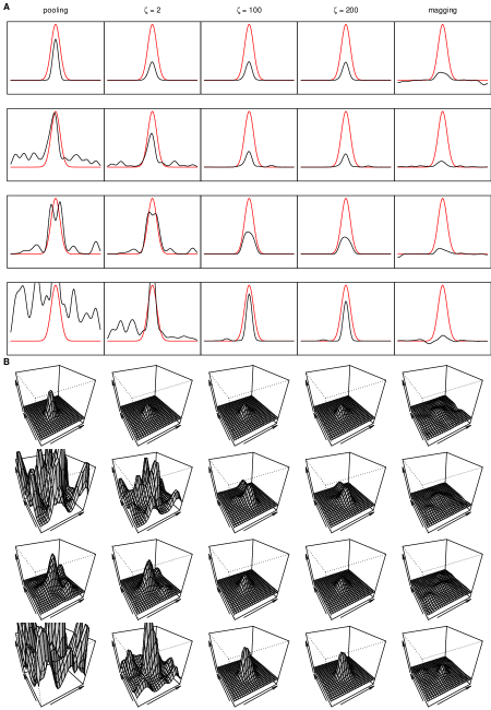
Figure 6: A: Temporal plots for $(x,y)=(12,12,)$. True signal $\phi(x,y,t)$ (red) and estimate $\hat{Y}_{x,y,t}$ (black) for model no. 10. Columns left to right; pooling, soft maximin $\zeta\in\{2,100,200\}$ and magging. Each row corresponds to a training set with 14 groups. B: Spatial plots for $t=50$ of the estimates from panel A.

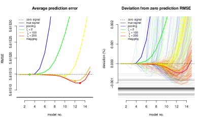
Figure 7: Left: Average RMSE across 70 test sets as a function of model complexity (model no.). Zero signal (dashed), true signal (black), pooled estimator (blue), soft maximin $\zeta=2$ (green), soft maximin $\zeta=100$ (orange), soft maximin $\zeta=200$ (red) and magging (yellow). The minimum is indicated with a bullet. Right: Deviation in RMSE relative to the zero prediction RMSE (percentage difference) for each method and on each test set (thin lines), as a function of model complexity. The corresponding averages are indicated with a thick line of the same color.

The right display in Figure 7 illustrates the variability in prediction accuracy for the different methods using their relative deviation in RMSE from that of the zero prediction. The low $\zeta$ estimators (pooled and $\zeta=2$) display high variability, reflecting a tendency to overfit group specific signals in the data. The high $\zeta$ soft maximin estimators and magging show much less variability. This underlines the robustness of the estimation methodology.

We note that only the high $\zeta$ methods succeed in extracting a common signal that is significantly more accurate than the zero prediction.

We note that while the gain in prediction performance, relative to the zero prediction is small, due to the low signal to noise ratio, it is not insignificant in terms of the quality of the extracted signal as illustrated in Figure 6. Here, the fit on four different training sets are displayed, and we observe directly how the low $\zeta$ methods tend to fit group fluctuation compared to the high $\zeta$ methods.

We quantify this by computing the average of the root mean squared signal error $\|\hat{Y}_{x,s}-\phi\|_{2}/\sqrt{m}$ made by the prediction obtained by training on set $s$ using method $x$. The left display in Figure 8 shows the result for each method $x$ and set $s$ as a function of model complexity as well as the average over $s$ (folds) and confirms the impression from Figure 6 and Figure 7.

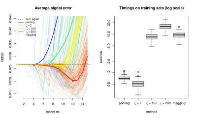
Figure 8: Left: mean squared signal error based on each of the 70 training set. Pooled estimator (blue), soft maximin $\zeta=2$ (green), soft maximin $\zeta=100$ (orange), soft maximin $\zeta=200$ (red) and magging (yellow). Right: Summary of run times (log scale) for the 70 training sets for each method.

Finally, the right display in Figure 8 shows how each method performs in terms of run time. In this setting given the average response across the 14 groups in a fold, computing the pooled estimator has the same complexity as computing one group fit in the magging procedure. Not surprisingly the pooled estimator (0.8 s) is roughly 12 times faster than magging (9.7 s), and also faster than the high $\zeta$ methods (8.1 s resp. 16.6 s). However, the soft maximin estimator with $\zeta=2$ (0.5 s) is faster than the pooled least square estimator.

5 Discussion

The maximin estimator with the $\ell_{1}$-penalty, as defined in Meinshausen and Bühlmann (2015), solves the minimization problem

$$\hat{\beta}_{mm}:=\arg\min_{\beta}\max_{g}\{-\hat{V}_{g}(\beta)\}+\lambda\|\beta\|_{1}.$$ (27)

Though the objective function is convex, it is nondifferentiable as well as nonseparable, and contrary to the claim in Section 4 of Meinshausen and Bühlmann (2015), coordinate descent will not always solve (27), see Tseng and Yun (2009).

Two approximate approaches for solving (27) were suggested in Meinshausen and Bühlmann (2015). The first, also a smooth approximation of the term $\max_{g}\{-\hat{V}_{g}(\beta)\}$, however, appears theoretically invalid and we did not find it to work in practice either. The second approximation, the maximal penalty solution, obtains a solution to (27) for the maximum $\lambda$ that yields a non-zero solution (at least one active feature) to (27). This solution is appropriate as an efficient initial estimator and clearly much cruder than a finely tuned maximin (type) estimator.

We note in passing that the solution path of (27) is piecewise linear in $\lambda$, and it may thus be computed using a method like LARS, see Roll (2008). A LARS-type algorithm or a coordinate descent algorithm of a smooth majorant, such as the soft maximin loss, has subsequently also been proposed to us by Meinshausen (personal communication) as better alternatives to those suggested in Meinshausen and Bühlmann (2015). In our experience, the LARS-type algorithm scales poorly with the size of the problem, and neither LARS nor coordinate descent can exploit the array-tensor structure.

We have developed soft maximin estimation as an alternative to maximin estimation that retains desirable statistical properties and is computationally more efficient. Furthermore the soft maximin parameter $\zeta$ controls the tradeoff between groups with large explained variance and groups with small explained variance leading to an interpolation of pooled estimation and maximin estimation. The gradient representation (10) shows explicitly how this tradeoff works: the gradient of the soft maximin loss is a convex combination of the gradients of the group-wise loss functions with weights controlled by $\zeta$. The largest weights are on those groups with the smallest explained variances and as $\zeta\to\infty$ the weights concentrate on the groups with minimal explained variance.

On the bike sharing data we have illustrated this interpolation property and the benefit of having a spectrum of estimators available instead of only the extremes (pooling resp. maximin). Notably, the optimal value of $\zeta$ in terms of prediction accuracy depends on the data context. Specifically we conclude that for heterogeneous data (hard) maximin estimator is not necessarily the best choice. Instead by tuning $\zeta$ e.g. by cross validation it might be possible to obtain an estimator in the spectrum between hard maximin and pooling that works better for the specific context. We note that a similar interpolation idea for heterogenous data has recently been proposed in the so called anchor regression framework, see Rothenhäusler et al. (2021).

On the simulated data (see also the neuronal VSDI data in Appendix B) it was demonstrated how the soft maximin estimator was able to extract a signal, and how the choice of the tuning parameter $\zeta$ affects the extracted signal and the prediction performance. In particular the simulations showed that soft maximin estimation ($\zeta\in\{100,200\}$) was able to extract a signal even in the presence of large heterogeneous noise components where the other methods (pooling and magging) failed.

In addition, we note that magging, proposed in Bühlmann and Meinshausen (2016) as a computationally attractive and generic alternative to (27) for estimation of maximin effects, in our numerical experiment, is not faster than using the soft maximin estimator.

In summary our proposed algorithm provides a means for approximately minimizing (27) and is as such an alternative to magging as an estimator of the maximin effect. More importantly, by the introduction of the tuning parameter $\zeta$ in the soft maximin loss we not only achieved an approximate solution of (27) but an interpolation between the (hard) maximin estimator and the pooled WLS estimator.

We expect that soft maximin estimation will be practically useful in a number of different contexts, as a way of aggregating explained variances across groups. In particular because it down-weights groups with a large explained variance that might simply be outliers, while it does not go to the extreme of the maximin effect, that can kill the signal completely.

Appendix A Proofs

Proof of Lemma 1.

i) Since $x_{g}=\max\{x_{1},\ldots,x_{G}\}$ for some $g\in\{1,\ldots,G\}$,

$$\max\{x_{1},\ldots,x_{G}\}=\frac{\log(e^{\zeta x_{g}})}{\zeta}\leq\frac{\log(e^{\zeta x_{g}}+\sum_{j\neq g}e^{\zeta x_{j}})}{\zeta}=\mathrm{lse}(x)$$

and also

$$\mathrm{lse}(x)\leq\frac{\log(\sum_{j}e^{\zeta x_{g}})}{\zeta}=\frac{\log(Ge^{\zeta x_{g}})}{\zeta}=\frac{\log(G)}{\zeta}+\max\{x_{1},\ldots,x_{G}\},$$

and the statement follows.

ii) From l’Hopitals rule we get

$$\lim_{\zeta\downarrow 0}\frac{\log(\frac{1}{G}\sum_{j}e^{\zeta x_{j}})}{\zeta}=\lim_{\zeta\downarrow 0}\Big{(}\frac{1}{G}\sum_{j}x_{j}e^{\zeta x_{j}}\Big{)}\Big{(}\frac{1}{G}\sum_{j}e^{\zeta x_{j}}\Big{)}^{-1}=\frac{1}{G}\sum_{j}x_{j},$$

implying

$$\mathrm{lse}(x)=\frac{\log(G)}{\zeta}+\frac{\log(\frac{1}{G}\sum_{j}e^{\zeta x_{j}})}{\zeta}=\frac{\log(G)}{\zeta}+\frac{1}{G}\sum_{j}x_{j}+o(1),$$

for $\zeta\downarrow 0$. ∎

Proof of Proposition 1.

First note that for any $\beta\in\mathbb{R}^{p}$ and any $g\in\{1,\ldots,G\}$

$$-\hat{V}_{g}(\beta) =\beta^{\top}\hat{\Sigma}_{g}\beta-2\beta^{\top}\hat{\Sigma}_{g}b_{g}-\frac{2\beta^{\top}\boldsymbol{X}_{g}^{\top}\boldsymbol{\epsilon}_{g}}{n_{g}}$$

$$=-V_{b_{g}}(\beta)+\beta^{\top}(\hat{\Sigma}_{g}-\Sigma)\beta-2\beta^{\top}(\hat{\Sigma}_{g}-\Sigma)b_{g}-\frac{2\beta^{\top}\boldsymbol{X}_{g}^{\top}\boldsymbol{\epsilon}_{g}}{n_{g}}$$

$$\geq-V_{b_{g}}(\beta)-\|\beta\|_{1}^{2}D-2\|\beta\|_{1}\max_{g}\|b_{g}\|_{1}D-2\|\beta\|_{1}\delta$$ (28)

and correspondingly

$$-\hat{V}_{g}(\beta) \leq-V_{b_{g}}(\beta)+\|\beta\|_{1}^{2}D+2\|\beta\|_{1}\max_{g}\|b_{g}\|_{1}D+2\|\beta\|_{1}\delta.$$ (29)

By assumption $\max_{g}\|b_{g}\|_{1}\leq\kappa$, and if also $\|\beta\|_{1}\leq\kappa$ we can write

$$\mathrm{lse}_{\zeta}(-V(\beta))-3\kappa^{2}D-2\kappa\delta \leq\mathrm{lse}_{\zeta}(-\hat{V}(\beta))$$ (30)

$$\leq\mathrm{lse}_{\zeta}(-V(\beta))+3\kappa^{2}D+2\kappa\delta,$$ (31)

by (A) and (29) and the properties of $\mathrm{lse}_{\zeta}$.

Let $H$ denote the convex hull of $\{b_{1},\ldots,b_{g}\}$. By Theorem 1 in Meinshausen and Bühlmann (2015) we know that $b^{\ast}\in H$ and since $\max_{g}\|b_{g}\|_{1}\leq\kappa$ we also have $\|b^{\ast}\|_{1}\leq\kappa$. By (7) it follows that

$$\mathrm{lse}_{\zeta}(-\hat{V}(\hat{\beta}_{smm}^{\kappa}))\leq\mathrm{lse}_{\zeta}(-\hat{V}(b^{\ast})).$$ (32)

Using (30) and (31) on respectively the left and right hand side of (32), yields

$$\mathrm{lse}_{\zeta}(-V(\hat{\beta}_{smm}^{\kappa})) \leq\mathrm{lse}_{\zeta}(-V(b^{\ast}))+6\kappa^{2}D+4\kappa\delta.$$ (33)

Applying Lemma 1 on both left and right hand side of (33) finally yields

$$\max_{g}\{-V_{b_{g}}(\hat{\beta}_{smm}^{\kappa})\} \leq\max_{g}\{-V_{b_{g}}(b^{\ast})\}+6\kappa^{2}D+4\kappa\delta+\frac{\log(G)}{\zeta}.$$ (34)

For the last statement, note that for fixed $\beta\in\mathbb{R}^{p}$, since $b\mapsto-V_{b}(\beta)$ is affine

$$\max_{g}\{-V_{b_{g}}(\beta)\}=\max_{b\in H}\{-V_{b}(\beta)\}.$$ (35)

An implication of Theorem 1 in Meinshausen and Bühlmann (2015) is $(b^{\ast})^{\top}\Sigma b\geq(b^{\ast})^{\top}\Sigma b^{\ast},\forall b\in H$, which combined with (35) shows

$$\max_{g}\{-V_{b_{g}}(b^{\ast})\}=\max_{b\in H}\{(b^{\ast})^{\top}\Sigma b^{\ast}-2(b^{\ast})^{\top}\Sigma b\}=-(b^{\ast})^{\top}\Sigma b^{\ast}.$$ (36)

Using $b^{\ast}\in H$ and (35), on the left hand side of (34), and using (36) on the right hand side of (34), gives us

$$(\hat{\beta}_{smm}^{\kappa})^{\top}\Sigma\hat{\beta}_{smm}^{\kappa}-2(\hat{\beta}_{smm}^{\kappa})^{\top}\Sigma b^{\ast}\leq-(b^{\ast})^{\top}\Sigma b^{\ast}+6\kappa^{2}D+4\kappa\delta+\frac{\log(G)}{\zeta},$$

which can be rearranged to yield the statement. ∎

To prove Proposition 2 we need the following technical lemma.

Lemma 2.

Assume $\sum_{i}w_{i}=1$ and $h_{i}\in\mathbb{R}^{p}$, $i\in\{1,\ldots,G\}$, $G\in\mathbb{N}$. Then

$$\sum_{i}w_{i}h_{i}\Big{(}h_{i}^{\top}-\sum_{j}w_{j}h_{j}^{\top}\Big{)}=\sum_{i}\sum_{j>i}w_{i}w_{j}(h_{i}-h_{j})(h_{i}-h_{j})^{\top}.$$

Proof.

First note that since $1-w_{i}=\sum_{j\neq i}w_{j}$

$$\sum_{i}w_{i}h_{i}\Big{(}h_{i}^{\top}-\sum_{j}w_{j}h_{j}^{\top}\Big{)} =\sum_{i}w_{i}h_{i}\Big{(}(1-w_{i})h_{i}^{\top}-\sum_{j\neq i}w_{j}h_{j}^{\top}\Big{)}$$

$$=\sum_{i}\sum_{j\neq i}w_{i}w_{j}h_{i}(h_{i}-h_{j})^{\top}.$$

Letting $a_{i,j}=w_{i}w_{j}h_{i}(h_{i}-h_{j})^{\top}$ we find that

$$\sum_{i}\sum_{j\neq i}a_{i,j} =\sum_{i}\sum_{j>i}a_{i,j}+\sum_{i}\sum_{i>j}a_{i,j}$$

$$=\sum_{i}\sum_{j>i}a_{i,j}+\sum_{j}\sum_{i>j}a_{i,j}\quad(\text{interchange summation order})$$

$$=\sum_{i}\sum_{j>i}a_{i,j}+\sum_{i}\sum_{j>i}a_{j,i}\quad(\text{relabel summation indices})$$

$$=\sum_{i}\sum_{j>i}w_{i}w_{j}(h_{i}-h_{j})(h_{i}-h_{j})^{\top},$$

where we used that $a_{j,i}=-w_{i}w_{j}h_{j}(h_{i}-h_{j})^{\top}$. ∎

Proof of Proposition 2.

First it is straightforward to compute the gradient of the loss

$$\nabla l_{\zeta}(\beta) =\frac{\sum_{j=1}^{G}e^{\zeta h_{j}(\beta)}\nabla\zeta h_{j}(\beta)}{\zeta\sum_{j=1}^{G}e^{\zeta h_{j}(\beta)}}$$

$$=e^{-\log(\sum_{j=1}^{G}e^{\zeta h_{j}(\beta)})}\sum_{j=1}^{G}e^{\zeta h_{j}(\beta)}\nabla h_{j}(\beta)$$

$$=\sum_{j=1}^{G}w_{j,\zeta}(\beta)\nabla h_{j}(\beta).$$ (37)

Then since

$$w_{j,\zeta}(\beta)=\frac{e^{\zeta h_{j}(\beta)}}{\sum_{i=1}^{G}e^{\zeta h_{i}(\beta)}}\geq 0$$

we see that $\sum_{j}w_{j,\zeta}(\beta)=1$ and conclude that the weights $w_{\zeta}(\beta)$ are convex for any $\beta$ and $\zeta$.

Differentiating (37) gives us

$$\nabla^{2}l_{\zeta}(\beta) =\sum_{j=1}^{G}\nabla h_{j}(\beta)\nabla w_{j,\zeta}(\beta)^{\top}+\sum_{j=1}^{G}w_{j,\zeta}(\beta)\nabla^{2}h_{j}(\beta).$$

Using the definition of $w_{j,\zeta}$ and (37) the first term is equal to

$$\sum_{j=1}^{G}w_{j,\zeta}(\beta)\nabla h_{j}(\beta)\Big{(}\nabla h_{j}(\beta)^{\top}-\sum_{i=1}^{G}w_{i,\zeta}(\beta)\nabla h_{i}(\beta)^{\top}\Big{)}$$

$$=\sum_{j=1}^{G}\sum_{i>j}w_{j,\zeta}(\beta)w_{i,\zeta}(\beta)(\nabla h_{j}(\beta)-\nabla h_{i}(\beta))(\nabla h_{j}(\beta)-\nabla h_{i}(\beta))^{\top}$$

where the equality follows from Lemma 2 since $(w_{j,\zeta}(\beta))_{j}$ are convex weights.

For a twice continuously differentiable function $f$ it holds that $f$ is strongly convex with parameter $\nu>0$ if and only if $\nabla^{2}f-\nu I$ is positive semi definite. Assuming all $h_{i}$ are convex and at least one is $\nu$-strongly convex it follows directly from (11) that $l_{\zeta}$ is also $\nu$-strongly convex.

Finally, the Hessian of $e^{l_{\zeta}(\beta)}$ is

$$\nabla^{2}e^{l_{\zeta}(\beta)}=\nabla^{2}l_{\zeta}(\beta)e^{l_{\zeta}(\beta)}+\nabla_{\beta}l_{\zeta}(\beta)\nabla_{\beta}l_{\zeta}(\beta)^{\top}e^{l_{\zeta}(\beta)}$$

where $\nabla_{\beta}l_{\zeta}(\beta)\nabla_{\beta}l_{\zeta}(\beta)^{\top}e^{l_{\zeta}(\beta)}$ is positive semi-definite for all $\beta$. Letting $m=\min_{\beta}l_{\zeta}(\beta)\in\mathbb{R}$, we have $e^{l_{\zeta}(\beta)}\geq e^{m}>0$ for all $\beta$ and must have $\nabla^{2}e^{l_{\zeta}(\beta)}-\tilde{\nu}I$ is positive semi definite for some $\tilde{\nu}>0$, showing that $e^{l_{\zeta}}$ is strongly convex. ∎

Proof of Corollary 1.

Let $\|\cdot\|_{d}$ denote the 2-norm on $\mathbb{R}^{d}$ and $A$ be a $d_{1}\times d_{2}$ matrix. Then $\vvvert A\vvvert_{d_{1},d_{2}}:=\sup_{v:\|v\|_{d_{2}}=1}\|Av\|_{d_{1}}$ is the sub-multiplicative matrix (operator) norm induced by the 2-norms on $\mathbb{R}^{d_{1}}$ and $\mathbb{R}^{d_{2}}$. For $a\in\mathbb{R}^{d_{1}}$ and $b\in\mathbb{R}^{d_{2}}$ note that $\vvvert a\vvvert_{d_{1},1}=\|a\|_{d_{1}}$ (Cauchy-Schwarz) and we get

$$\vvvert ab^{\top}\vvvert=\sup_{v:\|v\|_{d_{2}}=1}\|ab^{\top}v\|_{d_{1}}=\sup_{v:\|v\|_{d_{2}}=1}\|a\|_{d_{1}}|b^{\top}v|=\|a\|_{d_{1}}\|b\|_{d_{2}}.$$

Now suppressing subscripts observe that $\vvvert\nabla^{2}h_{g}(\beta)\vvvert=2\vvvert\boldsymbol{X}^{\top}\boldsymbol{X}\vvvert/m$ and $\nabla h_{i}(\beta)-\nabla h_{j}(\beta)=2\boldsymbol{X}^{\top}(\boldsymbol{Y}_{i}-\boldsymbol{Y}_{j})/m$. Then by Proposition 2 it follows that

$$\vvvert\nabla^{2}l_{\zeta}(\beta)\vvvert \leq\sum_{i}\sum_{j>i}w_{i,\zeta}(\beta)w_{j,\zeta}(\beta)\vvvert(\nabla h_{i}(\beta)-\nabla h_{j}(\beta))(\nabla h_{i}(\beta)-\nabla h_{j}(\beta))^{\top}\vvvert$$

$$\phantom{\leq}+\sum_{j}w_{j,\zeta}(\beta)\vvvert\nabla^{2}h_{j}(\beta)\vvvert$$

$$=\frac{4}{m^{2}}\sum_{i}\sum_{j>i}w_{i,\zeta}(\beta)w_{j,\zeta}(\beta)\|\boldsymbol{X}^{\top}(\boldsymbol{Y}_{i}-\boldsymbol{Y}_{j})\|^{2}+\frac{2\vvvert\boldsymbol{X}^{\top}\boldsymbol{X}\vvvert}{m}$$

$$\leq\frac{4}{m^{2}}\max_{i,j}\|\boldsymbol{X}^{\top}(\boldsymbol{Y}_{i}-\boldsymbol{Y}_{j})\|^{2}+\frac{2\vvvert\boldsymbol{X}^{\top}\boldsymbol{X}\vvvert}{m}$$

$$\leq\frac{4\vvvert\boldsymbol{X}^{\top}\boldsymbol{X}\vvvert}{m^{2}}\Big{(}\max_{i,j}\|\boldsymbol{Y}_{i}-\boldsymbol{Y}_{j}\|^{2}+\frac{m}{2}\Big{)}$$

using the properties of the matrix norm. By the mean value theorem it follows that $\nabla l_{\zeta}$ is Lipschitz continuous with the claimed bound. ∎

Proof of Proposition 3.

If we can show that Assumption A.1 from Chen et al. (2016) holds for the soft maximin problem (8) we can use Theorem A.1 in Chen et al. (2016) (or Lemma 4 in Wright et al. (2009)) to show that the sequence has an accumulation point. Theorem 1 in Wright et al. (2009) then establishes this accumulation point as a critical point for $F_{\zeta}=l_{\zeta}+\lambda J$.

Let $\Delta>0$, $\beta_{0}\in\mathbb{R}^{p}$ , and define the set

$$A_{0} =\{\beta:F_{\zeta}(\beta)\leq F_{\zeta}(\beta_{0})\}$$

$$A_{0,\Delta} =\{\beta:\|\beta-\beta^{\prime}\|\leq\Delta,\beta^{\prime}\in A_{0}\}.$$

A.1(i): $l_{\zeta}$ is $\nu$-strongly convex by Proposition 2 and since $J$ is assumed convex it follows that $F_{\zeta}$ is strongly convex. So $A_{0}$ is compact hence $A_{0,\Delta}$ is compact as a closed neighbourhood of $A_{0}$. As $l_{\zeta}$ is $C^{\infty}$ everywhere, $\nabla l_{\zeta}$ is Lipschitz on $A_{0,\Delta}$.

A.1(ii): Is satisfied by assumptions on $J$.

A.1(iii): Clearly $F_{\zeta}\geq 0$. Furthermore $F_{\zeta}$ is continuous hence uniformly continuous on the compact set $A_{0}$.

A.1(iv) $\sup_{\beta\in A_{0}}\|\nabla l_{\zeta}\|<\infty$ as $A_{0}$ is compact and $\nabla l_{\zeta}$ is continuous. Moreover, $\sup_{\beta\in A_{0}}\|J\|<\infty$ as $A_{0}$ is compact and $J$ is continuous. Finally, also $\inf J=0$. ∎

Appendix B Brain imaging data

The neuronal activity recordings were obtained using voltage-sensitive dye imaging (VSDI) in an experiment previously described in Roland et al. (2006). In short part of the visual cortex of a live ferret was exposed and stained with voltage-sensitive dye. Changes in membrane potential affects the dye and alters its fluorescence. The neuronal activity is recorded indirectly in terms of changes in the fluorescence using 464 photodiode channels organized in a two-dimensional (hexagonal) array. By padding with zeros the 464 channels were mapped to a $25\times 25$ matrix. We note the padding is chosen as the data is centred around zero implying the analysis is not altered by this manipulation. Alternatively observation weights can be used at a computational cost. During the trial (625 ms) an image was recorded every $0.6136$ ms. For 250 ms of the trial a visual stimulus, a white square on a grey screen, was presented to the ferret. A total of $G=275$ trials were recorded across 13 different ferrets.

Several sources of heterogeneity are potentially present in the raw data:

1. The heart beat affects the light emission by expanding the blood vessels in the brain, creating a cyclic heart rate dependent artefact. A changing heart rate over trials for one animal (fatigue) as well as differences in heart rate between animals will cause heterogeneity in the data.

2. Spatial inhomogeneities can arise due to differences in the cytoarchitectural borders between the animals causing misalignment problems.

3. The VSDI technique is very sensitive, see Grinvald and Bonhoeffer (2002). Even small changes in the experimental surroundings could affect the recordings and create heterogeneity.

4. Differences between animals in how they respond to the visual stimulus.

A trial with no visual stimulus (baseline), was recorded right before recording the stimulus trial. By aligning the baseline and stimulus trial, using an electrocardiography recording, the two recordings were subtracted to remove the heart rate artefact. We use this preprocessed data in the experiment.

Figure 9 shows recordings for five trials in the temporal dimension (panel A) and spatial dimension (panel B). Note that following the onset of the visual stimulus after 200 ms (first dashed line), the recordings are expected to show the result of a depolarization of the neuronal cells. Visual inspection of Figure 9 however does not reveal a clear stimulus response in every trial. We note the presence of variation that seems to be specific to the trial and could reflect the heterogeneity listed above.

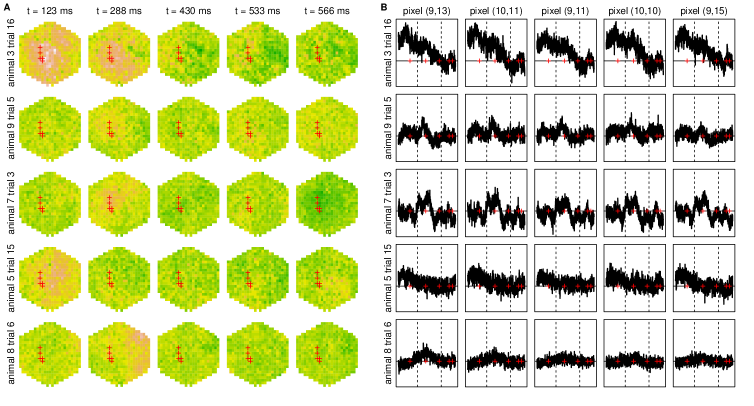
Figure 9: A: Spatial plots for five trials and five time points. The red crosses indicate the pixel time series shown in B. B: Temporal plots for the five same trials and five pixels indicated with red crosses in part A. The dashed lines indicate stimulus start and stop and red crosses indicate the time points plotted in part A.

B.1 Experiment setup

We use the array-tensor model from Section 3.2 with $p_{1}=p_{2}=9$ B-spline functions in each spatial dimension and $p_{3}=80$ B-splines in the temporal dimension. This gives us a model with marginal design matrices $\Phi_{1}$, $\Phi_{2}$, and $\Phi_{3}$, of sizes $25\times 9$, $25\times 9$ and $977\times 80$ respectively, given by the B-splines evaluations over the marginal domains. The model has $p=6480$ parameters.

We let one fold consist of all data from 2 out of the 13 animals. The model is trained on the fold and tested on data from the remaining 11 animals, for each method and each value of $\lambda$. We repeat this procedure $N:=\binom{13}{2}=78$ times, yielding 78 fitted models and corresponding test metrics for each method and each value of $\lambda$. Since the number of trials is not constant across animals the number of groups in each fold ranges from 23 to 80 (average is 42) giving us $14,044,375$ to $48,850,000$ (average $25,646,250$) observations in each fold.

B.2 Experimental results

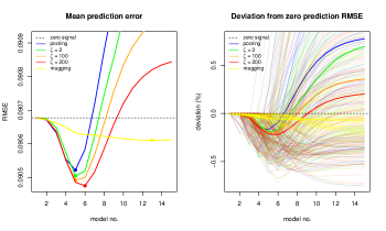
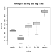
Figure 10: Top left: Average RMSE across 78 test sets as a function of model complexity (model no.). Zero signal (dashed), pooling (blue), soft maximin $\zeta\in\{2,100,200\}$ (resp. green, orange and red ) and magging (yellow). Top right: Deviation in RMSE relative to the zero prediction for each method and on each test set (thin lines), as a function of model complexity. Averages are indicated with a thick line of the same color. Bottom: Run times (log scale) for the 78 training sets for each method.

From the left display in Figure 10 we see that on average soft maximin with $\zeta=200$ (model no. 6) achieves the lowest over all out of sample RMSE. The low $\zeta$ estimators, pooled (model no. 5) and $\zeta=2$ (model no. 5) perform somewhat worse on average but still achieves significant reduction compared to the zero prediction. The approximate maximin estimator, magging estimator (model no. 13), performs the worst on this data in terms of RMSE.

Looking at Figure10 the low $\zeta$ methods show more variability than the high $\zeta$ methods and in particular are more prone to make predictions that are worse than the zero prediction. However the picture is not as clear as on the simulated data. We note that the magging estimator is quite consistently better than the zero prediction but not much, possibly reflecting the conservative nature of the hard maximin method.

Figure 10 also summarizes the timings for each method. Notably all the soft maximin estimators (8.9 s, 15.8 s and 18.7 s) outperform the pooled estimator (26.4 s) while also yielding better prediction accuracy (Figure 10). The magging estimator (931.4 s) suffers from having to compute individual fits for each group in the training set, making the the method orders of magnitudes slower in this case, without obtaining better accuracy. Note that the task alone of maximin aggregating the individual group estimates, by solving the associated quadratic programming problem, took on average 45 s. So even if fully parallelized the magging estimator is still computationally more demanding than the softmaximin estimator on this data set.

Appendix C Washington DC bike data

Here we show how to systematically determine the soft maximin parameter $\zeta$.

Owing to the temporal dependence in the data we will use a rolling cross validation scheme to systematically tune $\zeta$. We do this by training the model (24) on each set of six consecutive months and testing on the six following months. Following the experiment in section 4.1 we perform this rolling window CV in two ways; i) rolling forward from Jan 2011 to Dec 2012 and ii) rolling backwards from Dec 2012 to Jan 2011.

For i) and ii) respectively we then have 13 training and test pairs. We compute the soft maximin estimator on each of these training set for 50 values of $\zeta$ that range exponentially between 0.0001 and 0.3. On the corresponding test set we compute the mean squared prediction error.

Figure 11 shows the average prediction error (RMSE ) as a function of $\zeta$ for the forward rolling scheme i) and the backward rolling scheme ii) respectively. In line with section 4.1 in i) we see that low $\zeta$ values i.e. pooled OLS gives better predictions in terms of RMSE than higher values. For the experiment in ii) however $\zeta$ values around 0.03 yields the minimum prediction error.

Figure 11: Left: Average prediction error as a function of $\zeta$ obtained by the forward rolling cross validation procedure in experiment i). Right: Average prediction error as a function of $\zeta$ obtained by the backward rolling cross validation procedure in experiment ii)

We note that any conclusion will depend on the nature of the heterogeneity in the data as well as on how the cross validation is carried out, i.e. how the model is trained and tested. For the specific bike data set heterogeneity is not very pronounced and is easily explained in terms of increasing utilization of the bike sharing scheme. This causes an optimistic method like pooling to perform better over time than a conservative method like maximin. However we observe that the hard maximin (high $\zeta$) seems suboptimal in both experiments i) and ii) highlighting the benefit of computing a range of soft maximin estimators for a given data set.

C.1 Alternative models and grouping

Figure 12 shows the results with temperature temp and humidity hum added to (24). Results for this model are similar to the those in section 4.1 though with less pronounced gain in prediction robustness (Figure 12 B Bottom right).

We also group the data according to weathersit and fit the model

$$\sqrt{\texttt{cnt}_{i}}=\alpha_{0}+\sum_{j=1}^{10}\alpha_{j}\phi_{j}(\texttt{hr}_{i})+\sum_{j=1}^{5}\beta_{j}\phi_{j}(\texttt{weekday}_{i})+\sum_{j=1}^{5}\gamma_{j}\phi_{j}(\texttt{mnth}_{i})+\epsilon_{i}.$$ (38)

With this setup we obtain slightly higher 2011 prediction accuracy but less robust predictions (Figure 13 A and B bottom right).

Finally we also add temp and hum to (38). For this extended model the soft maximin estimator gives seemingly better 2011 predictions than the pooled estimator, see Figure 14.

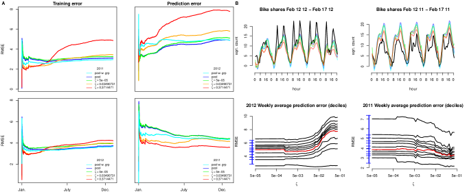
Figure 12: Results from fitting a model that includes temperature and humidity as covariates and using month as grouping.

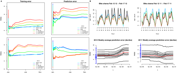
Figure 13: Results from fitting a model that use weathersit as grouping.

Figure 14: Results from fitting a model that includes temperature and humidity and use weathersit as grouping.

References

- Beck and Teboulle (2009) Beck, A. and M. Teboulle (2009). A fast iterative shrinkage-thresholding algorithm for linear inverse problems. SIAM Journal on Imaging Sciences 2(1), 183–202.
- Bühlmann and Meinshausen (2016) Bühlmann, P. and N. Meinshausen (2016). Magging: maximin aggregation for inhomogeneous large-scale data. Proceedings of the IEEE 104(1), 126–135.
- Buis and Dyksen (1996) Buis, P. E. and W. R. Dyksen (1996). Efficient vector and parallel manipulation of tensor products. ACM Transactions on Mathematical Software (TOMS) 22(1), 18–23.
- Chen et al. (2016) Chen, X., Z. Lu, and T. K. Pong (2016). Penalty methods for a class of non-lipschitz optimization problems. SIAM Journal on Optimization 26(3), 1465–1492.
- Currie et al. (2006) Currie, I. D., M. Durban, and P. H. Eilers (2006). Generalized linear array models with applications to multidimensional smoothing. Journal of the Royal Statistical Society: Series B (Statistical Methodology) 68(2), 259–280.
- De Boor (1979) De Boor, C. (1979). Efficient computer manipulation of tensor products. ACM Transactions on Mathematical Software (TOMS) 5(2), 173–182.
- Fanaee-T and Gama (2013) Fanaee-T, H. and J. Gama (2013). Event labeling combining ensemble detectors and background knowledge. Progress in Artificial Intelligence, 1–15.
- Grinvald and Bonhoeffer (2002) Grinvald, A. and T. Bonhoeffer (2002). Optical imaging of electrical activity based on intrinsic signals and on voltage sensitive dyes: The methodology.
- Lund (2018) Lund, A. (2018). glamlasso: Penalization in Large Scale Generalized Linear Array Models. R package version 3.0.
- Lund (2021) Lund, A. (2021). SMME: Soft Maximin Estimation for Large Scale Heterogeneous Data. R package version 1.0.1.
- Lund et al. (2017) Lund, A., M. Vincent, and N. R. Hansen (2017). Penalized estimation in large-scale generalized linear array models. Journal of Computational and Graphical Statistics 26(3), 709–724.
- Meinshausen and Bühlmann (2015) Meinshausen, N. and P. Bühlmann (2015). Maximin effects in inhomogeneous large-scale data. The Annals of Statistics 43(4), 1801–1830.
- Roland et al. (2006) Roland, P. E., A. Hanazawa, C. Undeman, D. Eriksson, T. Tompa, H. Nakamura, S. Valentiniene, and B. Ahmed (2006). Cortical feedback depolarization waves: A mechanism of top-down influence on early visual areas. Proceedings of the National Academy of Sciences 103(33), 12586–12591.
- Roll (2008) Roll, J. (2008). Piecewise linear solution paths with application to direct weight optimization. Automatica 44(11), 2732–2737.
- Rothenhäusler et al. (2021) Rothenhäusler, D., N. Meinshausen, P. Bühlmann, and J. Peters (2021). Anchor regression: Heterogeneous data meet causality. Journal of the Royal Statistical Society: Series B (Statistical Methodology) 83(2), 215–246.
- Tseng and Yun (2009) Tseng, P. and S. Yun (2009). A coordinate gradient descent method for nonsmooth separable minimization. Mathematical Programming 117(1-2), 387–423.
- Wright et al. (2009) Wright, S. J., R. D. Nowak, and M. A. Figueiredo (2009). Sparse reconstruction by separable approximation. IEEE Transactions on Signal Processing 57(7), 2479–2493.