Estimation of extreme survival probabilities with Cox model

Abstract.

We propose an extension of the regular Cox’s proportional hazards model which allows the estimation of the probabilities of rare events. It is known that when the data are heavily censored, the estimation of the tail of the survival distribution is not reliable. To improve the estimate of the baseline survival function in the range of the largest observed data and to extend it outside, we adjust the tail of the baseline distribution beyond some threshold by an extreme value model under appropriate assumptions. The survival distributions conditioned to the covariates are easily computed from the baseline. A procedure allowing an automatic choice of the threshold and an aggregated estimate of the survival probabilities are also proposed. The performance is studied by simulations and an application on two data sets is given.

Keywords: Survival probabilities, Extreme value theory, Adaptive estimation, Aggregation.

1. Introduction

The proportional hazards model introduced by [1] has been largely studied over the years and multiple extensions have been made to the original model. These developments often aim to make inference on the regression parameters in various setting including censoring, time-dependent coefficients, stratified and multistates models, missing and incomplete data etc. The references [2], [3], [4] and [5] give an overall view of this subject. The estimation of the underlying hazard functions is an important ingredient which mostly follows the interrogation of knowing the effect of a treatment. We refer to [6], [7] among others for an illustration. If we are in presence of a significant amount of censored data it is well known that we cannot predict with sufficient precision how the tail of the estimated survival distribution behaves near or beyond the last observed value. This is illustrated in the Figure 1 (top) using a real data example, where we can observe that the estimated baseline survival probability becomes constant in the long run.

The present paper aims to estimate the values of the survival distributions conditionally to a covariate in the Cox’s proportional hazards model in the case when the estimated probabilities are out of the range of the observed data by using extreme value modeling. Our analysis is based on the Peak-Over-Threshold method (see [8]), which allows to estimate the tail of a distribution beyond a threshold. Applications of this method can be seen in various domain such as insurance, biology, ecology, whether forecast etc. For insurance and financial applications, we can refer to [9] and [10] among many others. A rainfall data study can be found in [11] and high-frequency oyster data are studied in [12]. For some results related to the estimation of extreme values under random censoring without covariates we refer to [13], [14] and [15]. The case with covariates has been considered in [16], [17] and [18]. However, to the best of our knowledge, this approach was not used so far in the context of the Cox model with covariates.

Our idea is simple: we adjust a Pareto distribution for observations beyond a threshold, while the remaining part is estimated nonparametrically by the Nelson-Aalen estimator. The main difficulty is the appropriate choice of the threshold, which can be problematic as a large value will lead to an important variability and small value will increase the bias. This quandary is well known in theory of extreme values. To choose the threshold we make use of the adaptive procedure based on consecutive tests developed in [19]. In addition to this, we propose an aggregation procedure which allows to improve significantly the stability of the estimation. The performance of the proposed estimators is demonstrated by a simulation study and some applications are given. As an illustration in Figure 1 (bottom) we show the estimated baseline survival function by the proposed method.

The paper [20] deals also with the Cox model but in a very different way. In [20], the Cox model with qualitative covariates, say $z_{i}$ with a finite number of modalities is considered. Each modality has its own choice of the threshold $\widehat{\tau}$, which in principle are different. In the present paper we estimate only one threshold $\widehat{\tau}$ under the baseline distribution, which is automatically translated to the other modalities of the covariates. Thus we can deal with any type of covariates, and we have only one choice of the threshold. We also note that the paper [12] deals with a non stationary time series setting, where the goal is to estimate high quantiles driven by a non-parametricaly changing distribution function.

The paper is organized as follows. In Section 2, we introduce the notations, formulate the model and we state the main results. An explicit computation of the convergence rate using the Hall model is given as an example in Section 3. An automatic selection procedure of the threshold is stated in Section 4. In Section 5 we formulate our procedure for the aggregation of the estimated survival probabilities. A simulation study is done in Section 6 and an application on two data sets is given in Section 7.

2. Main results

2.1. Notations and model

Denote by $X$ a random variable representing the failure time, by $C$ a random variable representing the censoring time and by $Z$ a random covariate vector. We assume that $X$ and $C$ admit positive densities on $[x_{0},\infty)$, with $x_{0}\geq 0$ and that $X$ and $C$ are independent conditionally to $Z$. The observation time and failure indicator are respectively

$$T=\min\{X,C\}\quad\text{and}\quad\Delta=\mathbb{1}_{X\leq C},$$

where $\mathbb{1}$ is the indicator function. The Cox model (introduced by [1]) specifies that the hazard function of the failure time $X$ depends on the value $z$ of covariate vector $Z$ as follows:

$$h(\left.x\,\middle|\,z\right.)=\exp(\beta\cdot z)h_{0}(x),\ x\geq x_{0},$$

where $x_{0}\geq 0,$ $\beta$ is a vector of parameters, $h_{0}$ is an unknown baseline hazard function and $\beta\cdot z$ denotes the scalar product between $\beta$ and $z$. We denote by $f(\left.x\,\middle|\,z\right.)$ and $S(\left.x\,\middle|\,z\right.)=1-F(\left.x\,\middle|\,z\right.)$, respectively the density and survival functions of the failure time $X$ given $Z=z$. The hazard function $h(\left.x\,\middle|\,z\right.)$ is related to the functions $f(\left.x\,\middle|\,z\right.)$ and $S(\left.x\,\middle|\,z\right.)$ by the expressions

$$h(\left.x\,\middle|\,z\right.)=f(\left.x\,\middle|\,z\right.)/S(\left.x\,\middle|\,z\right.)$$

and

$$S(\left.x\,\middle|\,z\right.)=\exp(-\int_{x_{0}}^{x}h(\left.u\,\middle|\,z\right.)du).$$

Similarly, the hazard function of the censoring time is denoted by $h_{C}(\cdot)$, the density and survival function are respectively denoted $f_{C}(\cdot)$ and $S_{C}(\cdot)=1-F_{C}(\cdot)$. Let

(2.1) $$S_{0}(x)=S(\left.x\,\middle|\,0\right.)=\exp(-\int_{x_{0}}^{x}h_{0}(u)du)$$

be the baseline survival function. The survival function $S(\left.\cdot\,\middle|\,z\right.)$ is related to the baseline survival function $S_{0}(\cdot)$ by the expression

$$S(\left.x\,\middle|\,z\right.)=S_{0}(x)^{\exp(\beta\cdot z)}.$$

Assume that we observe a sequence of independent triples $(t_{i},\delta_{i},z_{i})$, $i=1,...,n$, where all $z_{i}$’s are nonrandom and each pair $(t_{i},\delta_{i})$ has the law of $(T,\Delta)$ given $Z=z_{i}$. In this paper we address the question of estimating the survival function $S(\left.x\,\middle|\,z\right.)$ for large values of $x$.

Let us explain the difficulties related to this problem using the classical Nelson-Aalen estimator. In the case when $x$ is larger than the last observed time $t_{\max}=\max\left\{t_{1},...,t_{n}\right\}$, the Nelson-Aalen estimator $\widehat{S}_{NA}(\left.\cdot\,\middle|\,z\right.)$ of $S(\left.\cdot\,\middle|\,z\right.)$ takes two positive constant values depending on the fact that the last observed time is censored or not. In Figure 1 (top) we plot the estimated baseline survival function $\widehat{S}_{NA}(\left.\cdot\,\middle|\,0\right.)$ for the commonly accessible bladder data set from R package survival (see Section 7.1 for details).

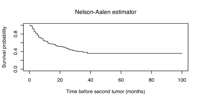
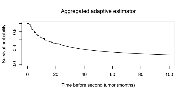
Figure 1. Estimated baseline survival probability (no-treatment) of the time of having the first recurrence of the bladder tumor: using the Nelson-Aalen estimator defined by (2.9) (top) and the adaptive aggregation defined by (5.2) (bottom).

Note that the Nelson-Aalen curve $\widehat{S}_{NA}(\left.t\,\middle|\,0\right.)$ becomes constant for $t\geq t_{\max}$. Moreover, as the survival times are heavily censored, the estimated survival probability $\widehat{S}_{NA}(\left.t\,\middle|\,0\right.)$ is far above $0$ for all $t\geq t_{\max}$. To overcome this effect, we assume some additional constraints on the survival function, which allow us to extrapolate it outside the available data range. Specifically, we assume the following condition:

C1.

We assume that $F_{0}$ belongs to the maximal domain of attraction of the Fréchet law with extreme value index $\theta>0$ which means that there exists two sequences $a_{n}>0$ and $b_{n}$ such that, for any $x\geq 0$,

$$F_{0}^{n}(a_{n}x+b_{n})\to\Phi_{\theta}(x)\ \mbox{as}\ n\to\infty,$$

where $\Phi_{\theta}(x)=e^{-x^{-\theta}},$ $x\geq 0$ is the Fréchet law and $F_{0}^{n}(x)=\mathbb{P}(\max_{1\leq i\leq n}{x_{i}}\leq x)$, with $x_{1},x_{2},\dots$ an i.i.d. sequence of random variables of common distribution $F_{0}$.

By the Fisher-Tippett-Gnedenko theorem (see Theorem 2.1 page 75 in [21]), condition (1) is equivalent to the property that for each $x\geq 1$,

(2.2) $$\frac{S_{0}(\tau x)}{S_{0}(\tau)}\to\left(x\right)^{-1/\theta}\ \text{as}\ \tau\to\infty.$$

As a consequence of (2.2) the following semi-parametric model is considered for the baseline survival function:

(2.3) $$S_{0,\tau,\theta}(x)=\left\{\begin{array}[]{ll}S_{0}\left(x\right)&\text{if\ \ }x\in[0,\tau],\\ S_{0}\left(\tau\right)\left(\frac{x}{\tau}\right)^{-1/\theta}&\text{if\ \ }x>\tau,\end{array}\right.$$

where the function $S_{0}$ is fully non-parametric, $\tau$ is a threshold parameter and the parametric part is completely described by the Pareto model with parameter $\theta.$ We denote the baseline hazard function of the previous model by

(2.4) $$h_{0,\tau,\theta}(x)=\left\{\begin{array}[]{ll}h_{0}\left(x\right)&\text{if\ \ }x\in[0,\tau],\\ \frac{1}{\theta x}&\text{if\ \ }x>\tau.\end{array}\right.$$

The corresponding cumulative hazard and survival function under the covariate constraint $Z=z$ are then respectively given by $H_{z,\tau,\theta}(x)=e^{\beta\cdot z}\int_{x_{0}}^{x}h_{0}\left(x\right)$ and

(2.5) $$S_{z,\tau,\theta}(x)=S(\left.x\,\middle|\,z,\tau,\theta\right.)=S_{0,\tau,\theta}(x)^{e^{\beta\cdot z}}.$$

For illustration purposes the estimated baseline survival function $S_{0}$ by the proposed model is given in Figure 1 (bottom), where for the estimation we have used the aggregation procedure with the adaptive choice of the threshold $\tau$ described in Section 5.2.

2.2. Estimators

In this section, we aim to provide the estimators necessary to deal with the model (2.3). To this end, we suppose the regression parameter $\beta$ of the Cox model known, for example, estimated by the standard procedure described in [1]. As to the threshold $\tau$, it is considered to be fixed (a selection procedure is presented latter on in Section 4). To estimate (2.3), we will combine the extreme value Hill type estimator of the parameter $\theta$ of the tail of the distribution function $F_{0}$ and the Nelson-Aalen non-parametric estimator of the baseline survival function $S_{0}.$

The joint density of the vector $(T,\Delta)$, given $Z=z$, is computed as

(2.6) $$p_{S_{0}}(\left.t,\delta\,\middle|\,z\right.)=(e^{\beta\cdot z}h_{0}(t))^{\delta}S_{0}(t)^{e^{\beta\cdot z}}f_{C}(t)^{1-\delta}S_{C}(t)^{\delta},$$

where $t\in[x_{0},\infty)$ and $\delta=\{0,1\}$. Denote by $p_{S_{0,\tau,\theta}}(\left.t,\delta\,\middle|\,z\right.)$ the joint density of the vector $(T,\Delta)$, given $Z=z$, when the survival function $S(\left.t\,\middle|\,z\right.)$ obeys the model (2.5):

$$p_{S_{0,\tau,\theta}}(\left.t,\delta\,\middle|\,z\right.)=(e^{\beta\cdot z}h_{0,\tau,\theta}(t))^{\delta}S_{0,\tau,\theta}(t)^{e^{\beta\cdot z}}f_{C}(t)^{1-\delta}S_{C}(t)^{\delta}.$$

Then the quasi-log-likelihood of the model is

$$\mathcal{L}(\left.\theta\,\middle|\,\mathbf{z}\right.)=\mathcal{L}(\left.\theta\,\middle|\,z_{1},...,z_{n}\right.)=\sum_{i=1}^{n}\ln p_{S_{0,\tau,\theta}}(\left.t_{i},\delta_{i}\,\middle|\,z_{i}\right.).$$

Removing the terms related to the censoring, the partial quasi-log-likelihood is

$$\mathcal{L}^{part}(\left.\theta\,\middle|\,\mathbf{z}\right.)=\sum_{i=1}^{n}\left(\delta_{i}\ln(h_{0,\tau,\theta}(t_{i}))+(\beta\cdot z_{i})\delta_{i}-e^{\beta\cdot z_{i}}\int_{x_{0}}^{t_{i}}h_{0,\tau,\theta}(u)du\right),$$

where the baseline hazard function $h_{0,\tau,\theta}(.)$ is defined by (2.4) and $\mathbf{z}=z_{1},\cdots,z_{n}$. Now, maximizing $\mathcal{L}^{part}(\left.\theta\,\middle|\,\mathbf{z}\right.)$ with respect to $\theta$, yields the estimator

(2.7) $$\widehat{\theta}_{\tau}=\frac{\sum_{t_{i}>\tau}e^{\beta\cdot z_{i}}\ln\left(\frac{t_{i}}{\tau}\right)}{\sum_{t_{i}>\tau}\delta_{i}}.$$

One can see that, the estimator is a transformation of the estimator introduced in [22].

The Nelson-Aalen estimator, suggested by [23] and rediscovered by [24], focus on estimating the cumulative hazard function $H_{0}(x)=\int_{0}^{x}h_{0}(t)dt$ by

$$\widehat{H}_{0}(t)=\sum_{t_{i}\leq t}\widehat{h}_{0}(t_{i}),$$

where, by maximizing the partial quasi-log-likelihood, we have

$$\widehat{h}_{0}(t_{i})=\frac{\delta_{i}}{\sum_{j=1}^{n}e^{\beta\cdot z_{j}}\mathds{1}_{t_{j}\geq t_{i}}}.$$

This estimator was suggested by [25]. The estimator of the survival function (2.3) is then given by

(2.8) $$\widehat{S}_{0,\tau,\widehat{\theta}_{\tau}}(t)=\left\{\begin{array}[]{cc}\widehat{S}_{0}\left(t\right)&\text{if\ \ }t\in[0,\tau],\\ \widehat{S}_{0}\left(\tau\right)\left(\frac{t}{\tau}\right)^{-1/\widehat{\theta}_{\tau}}&\text{if\ \ }t>\tau,\end{array}\right.$$

where the Nelson-Aalen non-parametric estimator of $S_{0}$ is defined by

(2.9) $$\widehat{S_{0}}\left(t\right)=e^{-\widehat{H}_{0}(t)}.$$

The estimator of the survival function (2.5) is then given by $\widehat{S}_{z,\tau,\theta}(t)=\widehat{S}_{0,\tau,\widehat{\theta}_{\tau}}(t)^{e^{\beta\cdot z}}$.

2.3. Consistency of $\widehat{\theta}_{\tau}$

In this section we state a general consistency result for the estimator $\widehat{\theta}_{\tau}$ of $\theta$, which we apply in Section 3 to obtain the rate of convergence under the Hall model. To state it, we need some notations.

The Kullback-Leibler divergence between two equivalent distributions, say $P$ and $Q$, is denoted $\mathcal{K}(P,Q)=\int\ln(dP/dQ)dP.$ This divergence, between two Pareto distributions with parameters $\theta^{\prime}$ and $\theta$, can be written as

(2.10) $$\mathcal{K}(\theta^{\prime},\theta)=\frac{\theta^{\prime}}{\theta}-1-\ln(\frac{\theta^{\prime}}{\theta})\sim\left(\frac{\theta^{\prime}}{\theta}-1\right)^{2}\quad\text{as}\quad\frac{\theta^{\prime}}{\theta}\to 1.$$

The $\chi^{2}$-entropy between the probability measures $P$ and $Q$ is defined by

(2.11) $$\chi^{2}(P,Q)=\int dP/dQdP-1.$$

The following theorem gives an estimate of the Kullback-Leibler entropy between $\widehat{\theta}_{\tau}$ and $\theta$ which is expressed in terms of the $\chi^{2}$-entropy between the two laws $P_{S_{0}}(\left..\,\middle|\,z_{i}\right.)$ and $P_{S_{0,\tau,\theta}}(\left..\,\middle|\,z_{i}\right.)$. The notation $a_{n}=O(b_{n})$ means that there is a positive constant $c$ such that $\mathbb{P}(a_{n}>cb_{n},b_{n}<\infty)\rightarrow 0$ as $n\rightarrow\infty$. In the sequel we denote by $\mathbb{P}$ the probability measure corresponding to the "true" model which has the baseline survival function $S_{0}$.

Theorem 2.1.

Assume that $S_{0}$ is an arbitrary survival function as defined by (2.1) and that $S_{0,\tau,\theta}$ satisfies the model (2.3). Then for any $\theta>0$, and $\tau\geq x_{0}$, we have

$$\mathcal{K}(\widehat{\theta}_{\tau},\theta)=O_{\mathbb{P}}\left(\frac{1}{\widehat{n}_{\tau}}\sum_{i=1}^{n}\chi^{2}(P_{S_{0}}(\left..\,\middle|\,z_{i}\right.),P_{S_{0,\tau,\theta}}(\left..\,\middle|\,z_{i}\right.))+\frac{4\ln(n)}{\widehat{n}_{\tau}}\right),$$

where $\widehat{n}_{\tau}=\sum_{t_{i}>\tau}\delta_{i}$.

Theorem 2.1 gives an upper bound of the Kullback-Leibler entropy which can be read in two parts, the bias term $\frac{1}{\widehat{n}_{\tau}}\sum_{i=1}^{n}\chi^{2}(P_{S_{0}}(\left..\,\middle|\,z_{i}\right.),P_{S_{0,\tau,\theta}}(\left..\,\middle|\,z_{i}\right.))$ and the variance term $\frac{4\ln(n)}{\widehat{n}_{\tau}}$.

Now, we formulate some sufficient conditions for the consistence of the estimator $\widehat{\theta}_{\tau}$. In order to estimate the bias term, we need to introduce a quantity which show how the censoring rate evolves with the threshold $\tau$, when we consider only the observations exceeding $\tau.$ For this, we introduce the following conditioned mean censoring rate function given $Z=z$:

$$\tau\mapsto q_{F}(\left.\tau\,\middle|\,z\right.)=\int_{\tau}^{\infty}\frac{S(\left.t\,\middle|\,z\right.)}{S(\left.\tau\,\middle|\,z\right.)}\frac{f_{C}(\left.t\,\middle|\,z\right.)}{S_{C}(\left.\tau\,\middle|\,z\right.)}dt\in[0,1],\quad\tau\geq x_{0}.$$

The value $q_{F}(\left.\tau\,\middle|\,z\right.)$ gives the rate of censored observations above the threshold $\tau$. In order to estimate the extreme survival probabilities it is natural to require that the rate of censored observations above the threshold $\tau$ is strictly less than $1$. We shall impose on $q_{F}(\left.\tau\,\middle|\,z\right.)$ the following condition:

C2.

There is a constant $q_{0}<1$ such that, for $\tau\geq x_{0}$ large enough,

$$q_{F}(\left.\tau\,\middle|\,z_{i}\right.)\leq q_{0},\quad i=1,...,n.$$

Condition (2) is easily verified, for instance, when both the distribution function of the survival time and that of the censoring time follow the Cox model and are in the maximal domain of attraction of the Fréchet law with parameters $\theta(z)$ and $\theta_{C}(z)$ respectively. Indeed, we show in the Lemma A.3 that, in this case, for any $z$,

$$q_{F}(\left.\tau\,\middle|\,z\right.)\to\frac{\theta(z)}{\theta(z)+\theta_{C}(z)}\ \mbox{as}\ \tau\to\infty.$$

where under some mild assumptions one can verify that

(2.12) $$\frac{\theta(z)}{\theta(z)+\theta_{C}(z)}\leq q_{0}<1.$$

In addition we introduce the following conditions:

C3.

There exists $z_{\min}$ and $z_{\max}$ such that

$$z\in\mathbb{Z}:=[z_{\min};z_{\max}].$$

C4.

Von-Mises condition:

$$th_{0}(t)\rightarrow\frac{1}{\theta}\quad\text{as}\quad t\rightarrow\infty.$$

It is well known that (4) implies condition (1), see [21]. For any $\tau>0$, set

$$\rho_{\tau}=\sup_{t>\tau}\left|th_{0}(t)-\frac{1}{\theta}\right|.$$

It is easy to see that the Von-Mises condition (4) is equivalent to the fact that there exists a sequence of thresholds $(\tau_{n})$ satisfying $x_{0}\leq\tau_{n}\to\infty$ as $n\to\infty$ such that $n\rho_{\tau_{n}}^{2}\rightarrow 0$ as $n\rightarrow\infty$.

The following result shows the consistency of the estimated parameter $\widehat{\theta}_{\tau_{n}}$:

Theorem 2.2.

Assume conditions (2), (3) and (4). For any sequence $(\tau_{n})$ satisfying

(2.13) $$x_{0}\leq\tau_{n}\to\infty,\quad n\rho_{\tau_{n}}^{2}\rightarrow 0\quad\text{as}\quad n\rightarrow\infty$$

and

(2.14) $$\sum_{i=1}^{n}S(\left.\tau_{n}\,\middle|\,z_{i}\right.)S_{C}(\left.\tau_{n}\,\middle|\,z_{i}\right.)\rightarrow\infty\quad\text{as}\quad n\rightarrow\infty,$$

it holds

$$\widehat{\theta}_{\tau_{n}}\xrightarrow[n\rightarrow\infty]{\mathbb{P}}\theta.$$

Condition (2.13) gives a control on the bias $\frac{1}{\widehat{n}_{\tau}}\sum_{i=1}^{n}\chi^{2}(P_{S_{0}}(\left..\,\middle|\,z_{i}\right.),P_{S_{0,\tau,\theta}}(\left..\,\middle|\,z_{i}\right.))$ of the model which should be small as $n\to\infty$, while condition (2.14) is responsible for the control of the variance $\frac{4\ln(n)}{\widehat{n}_{\tau}}$ of the model. We will show in the next section how to verify conditions (2), (2.13) and (2.14) with a large class of models.

3. Computation of the explicit rate of convergence for the Hall model

In this section we consider a model which is related to the families of distributions in [26], [27] and [19] for the extreme value estimation. The result of the Theorem A.4 in Section 2.3 shows that the rate of convergence of the estimator $\widehat{\theta}_{\tau_{n}}$ depends on the threshold $\tau_{n}$ and the survival functions of the survival and censoring times. To express the rate of convergence in terms of the sample size, some assumptions must be made on the survival functions $S$ and $S_{C}$.

C5.

The baseline hazard function $h_{0}$ is such that for some unknown parameter $\theta\in(\theta_{min},\theta_{max})$ and any $t>1,$

$$|th_{0}(t)-\frac{1}{\theta}|\leq c_{1}t^{-\frac{\alpha}{\theta}},$$

where $\alpha$, $c_{1}$, $\theta_{min}$ and $\theta_{max}$ are some positive constants.

Condition (5) means that $th_{0}(t)$ converges to $\frac{1}{\theta}$ polynomially fast as $t\rightarrow\infty$. Similarly we assume:

C6.

The hazard function $h_{C}$ of the censoring time $C$ is such that for any $z\in\mathbb{Z}:=[z_{\min};z_{\max}]$ and any $t>1,$

$$|th_{C}(\left.t\,\middle|\,z\right.)-\frac{1}{\theta_{C}(z)}|\leq c_{2}t^{-\mu},$$

where $\theta_{C}(z)=\frac{\theta}{\gamma}e^{-\beta\cdot z}$ and $\gamma>0$, $c_{2}>0$ and $\mu>1$ are some constants.

Theorem 3.1.

Assume condition (3), (5) and (6). Suppose in addition that $\frac{\varrho_{2}}{\varrho_{1}}\frac{1+\gamma}{1+\gamma+2\alpha}\leq 1,$ where $\varrho_{1}=\min_{\beta\cdot z}(e^{\beta\cdot z})$ and $\varrho_{2}=\max_{\beta\cdot z}(e^{\beta\cdot z})$. Then, there exists a constant $c$ such that,

$$\lim_{n\to\infty}\mathbb{P}\left(\mathcal{K}(\widehat{\theta}_{\tau_{n}},\theta)\leq c\left(\frac{\ln n}{n}\right)^{1-\frac{\varrho_{2}}{\varrho_{1}}\frac{1+\gamma}{1+\gamma+2\alpha}}\right)=1,$$

where

$$\tau_{n}=n^{\frac{\theta/\varrho_{1}}{1+\gamma+2\alpha}}\ln^{-\frac{\theta/\varrho_{1}}{1+\gamma+2\alpha}}n.$$

When the covariate $z$ is absent, say $z=0$, then $\varrho_{2}=\varrho_{1}=1$ and we recover the result of Theorem 4.2 of the paper [20], where it is shown that when $\gamma$ goes to $0$ (no censoring) the rate becomes close to the optimal rate of convergence $n^{\frac{2\alpha}{1+2\alpha}}$ in the context of the extreme value estimation, see [28] and [19]. In the case of a binary covariate (i.e. $z\in\{0,1\}$), if we assume that $\beta>0$, the convergence speed becomes $\mathcal{K}(\widehat{\theta}_{\tau_{n}},\theta)=O_{\mathbb{P}}\left((\frac{\ln n}{n})^{1-e^{\beta}\frac{1+\gamma}{1+\gamma+2\alpha}}\right)$ with $\tau_{n}=n^{\frac{\theta}{1+\gamma+2\alpha}}\ln^{-\frac{\theta}{1+\gamma+2\alpha}}n.$

Condition (6) may seem a bit cumbersome at first sight, however, with a closer look we see that it is quite natural if we want to obtain a close rate of convergence. To see this we note that condition (5) can be equivalently stated as

$$|th(\left.t\,\middle|\,z\right.)-\frac{1}{\theta(z)}|\leq c_{1}t^{-\frac{\alpha}{\theta(z)}},$$

where the tail index $\theta(z)=\theta e^{-\beta\cdot z}$ depends on the covariate $z$. Now conditions (2.12) and (2) will be verified with $q_{0}=\frac{\gamma}{\gamma+1}$.

Condition (6) can be replaced by the following condition:

C7.

The hazard function $h_{C}$ of the censoring time $C$ is such that for any $z\in\mathbb{Z}:=[z_{\min};z_{\max}]$ and any $t>1,$

$$|th_{C}(t)-\frac{\gamma}{\theta}|\leq c_{2}t^{-\mu},$$

where $\gamma>0$, $c_{2}>0$ and $\mu>1$ are some constants.

With (7) instead of (6) we can obtain the following result:

Theorem 3.2.

Assume condition (3), (5) and (7). Suppose in addition that $\frac{\varrho_{2}+\gamma}{\varrho_{1}+\gamma+2\alpha\varrho_{1}}\leq 1,$ where $\varrho_{1}=\min_{\beta\cdot z}(e^{\beta\cdot z})$ and $\varrho_{2}=\max_{\beta\cdot z}(e^{\beta\cdot z})$. Then, there exists a constant $c$ such that,

$$\lim_{n\to\infty}\mathbb{P}\left(\mathcal{K}(\widehat{\theta}_{\tau_{n}},\theta)\leq c\left(\frac{\ln n}{n}\right)^{1-\frac{\varrho_{2}+\gamma}{\varrho_{1}+\gamma+2\alpha\varrho_{1}}}\right)=1,$$

where

$$\tau_{n}=n^{\frac{\theta}{\varrho_{1}+\gamma+2\alpha\varrho_{1}}}\ln^{-\frac{\theta}{\varrho_{1}+\gamma+2\alpha\varrho_{1}}}n.$$

The proof of Theorem 3.2 is similar to that of Theorem 3.1 and therefore will not be given in this paper.

4. The selection of the threshold

It is well-known that the choice of the threshold $\tau$ has a major impact on the quality of the estimation in the extreme value modelling. We propose a data-driven choice of the threshold $\tau$ inspired by [19]. The adaptive threshold $\widehat{\tau}$ is selected by a sequential testing procedure followed by a selection using a penalized maximum likelihood.

Consider the following semi-parametric survival function consisting of three parts:

(4.1) $$S_{0,\tau,\theta,s,\lambda}(x)=\left\{\begin{array}[]{cc}S_{0}\left(x\right)&\text{if\ \ }x\in[0,s],\\ S_{0}\left(s\right)\left(\frac{x}{s}\right)^{-\frac{1}{\lambda}}&\text{if\ \ }x\in(s,\tau].\\ S_{0}\left(s\right)\left(\frac{\tau}{s}\right)^{-\frac{1}{\lambda}}\left(\frac{x}{\tau}\right)^{-\frac{1}{\theta}}&\text{if\ \ }x>\tau,\end{array}\right.$$

where $\lambda>0$, $\theta>0$ and $x_{0}<s<\tau$. The maximum quasi-likelihood estimators $\widehat{\theta}_{\tau}$ of $\theta$ and $\widehat{\lambda}_{s,\tau}$ of $\lambda$ are respectively given by (2.7) and

$$\widehat{\lambda}_{s,\tau}=\frac{\widehat{\theta}_{s}\widehat{n}_{s}-\widehat{\theta}_{\tau}\widehat{n}_{\tau}}{\widehat{n}_{s,\tau}},$$

where for brevity, we have denoted $\widehat{n}_{s}=\sum_{t_{i}>s}\delta_{i}$, $\widehat{n}_{\tau}=\sum_{t_{i}>\tau}\delta_{i}$ and $\widehat{n}_{s,\tau}=\sum_{s<t_{i}<\tau}\delta_{i}$.

Assume that the observations $t_{i}$ are ordered in the decreasing order such that $t_{1}>...>t_{n}$. We define a uniform grid $K$ in the subscripts $i=1,..,n$ of a size $n_{grid}$, say $K=\{k_{1},k_{2},...,k_{n_{grid}}\}$. The grid $K$ define the set of observations $\{t_{k_{1}},t_{k_{2}},...,t_{k_{n_{grid}}}\}$ on which the testing procedure will be performed.

We start with the first subscript $k=k_{1}$ on the grid $K$. For the subscript $k$ we test the null hypothesis

$$\mathcal{H}_{0}(t_{k})\quad\text{:}\quad S_{0}(x)=S_{0,t_{k},\theta}(x)$$

against the alternative hypothesis

$$\mathcal{H}_{1}(t_{k},t_{l})\quad\text{:}\quad S_{0}(x)=S_{0,t_{k},\theta,t_{l},\lambda}(x),$$

where $S_{0,t_{k},\theta}(x)$ is given by (2.3), $S_{0}(x)=S_{0,t_{k},\theta,t_{l},\lambda}(x)$ is given by (4.1), and $t_{l}$ can change between $t_{1}$ and $t_{k}$. If we choose all the $t_{l}$ between $t_{1}$ and $t_{k}$, some bias is introduced by the observations too close to $t_{1}$ and $t_{k}$. To overcome this problem, we introduce two parameters $\zeta^{\prime}$ and $\zeta^{\prime\prime}$ satisfying $0<\zeta^{\prime},\zeta^{\prime\prime}<0.5$ which are empirically calibrated. Now $t_{l}$ will be varying between $t_{(1-\zeta^{\prime\prime})k}$ and $t_{\zeta^{\prime}k}$.

The log-likelihood ratio test statistic used to test the null hypothesis $\mathcal{H}_{0}(t_{k})$ against the alternative $\mathcal{H}_{1}(t_{k},t_{l})$ is given by

(4.2) $$LR(t_{k},t_{l})=\widehat{n}_{t_{k},t_{l}}\mathcal{K}(\widehat{\lambda}_{t_{k},t_{l}},\widehat{\theta}_{t_{k}})+\widehat{n}_{t_{l}}\mathcal{K}(\widehat{\theta}_{t_{l}},\widehat{\theta}_{t_{k}}),$$

where $\mathcal{K}$ is the Kullback-Leibler divergence defined in Section 2.3. The test statistic is compared to a critical value $D$, which is also empirically calibrated. We test, for every $t_{l}\in[t_{(1-\zeta^{\prime\prime})k};t_{\zeta^{\prime}k}]$, the hypothesis $\mathcal{H}_{0}(t_{k})$ against the alternative $\mathcal{H}_{1}(t_{k},t_{l})$ and, if the critical value is not exceeded, we increase the subscript on the grid $K$ and preform the test with the next subscript on the grid $K.$ This will be repeated until the critical value is exceeded.

We denote by $\hat{k}$ the first subscript $k\in K$ for which the critical value $D$ is exceeded. Set $\widehat{s}=t_{\hat{k}}$, which is called in the sequel the breaking point. We aim to choose the adaptive threshold $\widehat{\tau}$ by maximizing the quasi-log-likelihood function

$$\underset{\theta}{\text{max}}\mathcal{L}^{part}(\left.\theta\,\middle|\,\mathbf{z}\right.)-\text{Pen}(\left.\widehat{\theta}_{\hat{s}}\,\middle|\,\mathbf{z}\right.)$$

$$\qquad=\mathcal{L}^{part}(\left.\widehat{\theta}_{\tau}\,\middle|\,\mathbf{z}\right.)-\text{Pen}(\left.\widehat{\theta}_{\hat{s}}\,\middle|\,\mathbf{z}\right.),$$

where $\text{Pen}(\left.\widehat{\theta}_{\hat{s}}\,\middle|\,\mathbf{z}\right.)$ is the penalty function defined by

(4.3) $$\text{Pen}(\left.\theta\,\middle|\,\mathbf{z}\right.)=\mathcal{L}^{part}(\left.\theta\,\middle|\,\mathbf{z}\right.).$$

Taking into account (4.3), it follows that the second term of (4.2) can be viewed as the penalized quasi-log-likelihood

(4.4) $$\mathcal{L}^{Pen}(s,\tau)=\mathcal{L}^{part}(\left.\widehat{\theta}_{\tau}\,\middle|\,\mathbf{z}\right.)-\text{Pen}(\left.\widehat{\theta}_{s}\,\middle|\,\mathbf{z}\right.).$$

We find the subscript which maximize the penalized quasi-log-likelihood

(4.5) $$\widehat{l}=\underset{\zeta^{\prime}\hat{k}\leq l\leq(1-\zeta^{\prime\prime})\hat{k}}{\mbox{argmax}}\mathcal{L}^{Pen}\left(\hat{s},t_{l}\right).$$

Finally, we set the adaptive threshold

(4.6) $$\widehat{\tau}=t_{\hat{l}}$$

and its associated parameter $\widehat{\theta}_{\hat{\tau}}$.

5. Aggregation

The transition between the non-parametric part and the parametric part in the model (2.3) can sometimes be rough, especially when the sample size is small. We propose two ways of smoothing the transition relying on a aggregating estimators corresponding to different thresholds.

5.1. Simple aggregation

The first aggregation we describe can be called ’simple aggregation’ as we aggregate the estimated cumulative hazard function from multiple thresholds. The procedure can be resumed with 3 simple steps, where the observations $t_{i}$ are ordered in the decreasing order such that $t_{1}>...>t_{n}$.

• Step 1. Choose $M\geq 1$ thresholds $\tau_{1}=t_{m_{0}},\dots,\tau_{m}=t_{m_{0}+M-1}$ from the observed values, where $m_{0}\geq 1.$

• Step 2. For each chosen threshold $\tau_{k}$ compute the estimated cumulative hazard function $\widehat{H}_{z,\tau_{k},\theta}(x)$.

• Step 3. Compute the simple aggregation estimator by

  (5.1) $$\widehat{S}_{\mbox{\scriptsize sa}}(\left.x\,\middle|\,z\right.)=\exp\left(-\frac{1}{M}\sum_{k=1}^{M}\widehat{H}_{z,\tau_{k},\theta}(x)\right).$$

For the algorithm to work, we need to choose $m_{0}$ as the first observation (censored or not) having at least one non-censored observation above it: $m_{0}\geq\min\{m:\sum_{t_{i}>t_{m}}\delta_{i}=1\}.$ With $M=1$ and $m_{0}=k$, the procedure becomes the estimation of the semi-parametric model (2.3) with a fixed threshold $\tau=t_{k}$.

5.2. Adaptive aggregation

The second aggregation we describe can be called ’adaptive aggregation’ as we aggregate cumulative hazard functions from the adaptive procedure described in Section 4. Let $l_{1},\dots,l_{N_{\hat{s}}}$ be the reversed ranks of the sequence

$$\mathcal{L}^{Pen}\left(t_{\hat{s}},t_{l}\right),\ \zeta^{\prime}\hat{s}\leq l\leq(1-\zeta^{\prime\prime})\hat{s},$$

where $N_{\hat{s}}$ is its cardinality and $\hat{s}$ is the breaking point computed by the adaptive procedure described in Section 4. For the adaptive aggregation we proceed in the same way as in the case of the simple aggregation described above. It can be resumed with the following steps:

• Step 1. Choose $M\geq 1$ thresholds $\tau_{1}=t_{l_{1}},\dots,\tau_{M}=t_{l_{M}}$ from the observed values.

• Step 2. For each chosen threshold $\tau_{l_{k}}$, compute the estimated cumulative hazard function $\widehat{H}_{z,\tau_{l_{k}},\theta}(x)$.

• Step 3. Compute the weights on the estimated cumulative hazard functions from the value of the penalized likelihood (4.4) by

  $$w_{l_{k}}=\mathcal{L}^{Pen}\left(t_{\hat{s}},t_{l_{k}}\right)/\sum_{i=1}^{M}\mathcal{L}^{Pen}\left(t_{\hat{s}},t_{l_{i}}\right).$$

• Step 4. Compute the adaptive aggregation estimator by

  (5.2) $$\widehat{S}_{\mbox{\scriptsize aa}}(\left.x\,\middle|\,z\right.)=\exp\left(-\sum_{k=1}^{M}w_{l_{k}}\widehat{H}_{z,\tau_{l_{k}},\theta}(x)\right).$$

Note that with $M=1$, the procedure becomes the estimation of the semi-parametric model (2.3) with the adaptive threshold $\tau$ chosen from the procedure described in Section 4.

6. Simulation study

We carry a simulation study to evaluate how the proposed estimators behave against the usual Nelson-Aalen estimator. We are interested in the values of the baseline survival probability $S_{0}(x)$ when $x$ is large. To compare the estimations, we use the relative mean square error (RelMSE), which we define as $RelMSE_{\widehat{S_{0}}(x)}=\mathbb{E}\left(\ln^{2}\frac{\widehat{S}_{0}(x)}{S_{0}(x)}\right)$. One can compare the estimated survival function and the true survival function for any $z$ by multiplying the error for the baseline by $e^{2\beta.z}$. We also look at the ratio between the estimators proposed in this paper and the Nelson-Aalen estimator. The parameters of the adaptive procedure in Section 4 are set to the following values $n_{\text{grid}}=100$, $\zeta^{\prime}=0.25$, $\zeta^{\prime\prime}=0.05$. A simulation study has been performed in [12] concerning the choice of these parameters and led to these values.

The study of the properties of the adaptive estimators introduced in Sections 4 and 5 is outside the scope of this paper. However, we shall discus briefly the choice of the critical value $D$, as this seems to be one of the sensitive points of the proposed adaptive procedure in Section 4. In our paper the critical value is calibrated under the hypothesis that the true distribution $F$ is fully parametric and follows a Pareto distribution with some parameter $\theta$ and so does not depend on $F_{T}$ nor $F_{C}$. We note in addition that, as it is shown in [19], the law of the test statistic (4.2) does not depend on the parameter $\theta$, and therefore, we can choose $\theta=1$. It is also argued in [19] that the obtained critical value remains stable with the change of the number of observations. If we suppose for a moment that we introduce censoring in the model, at least from the intuitive point of view, it will act as a reducer of the number of extreme observations, so by the previous remark the critical value will remain stable. Moreover, it was also observed that the adaptive choice $\widehat{\tau}$ remains stable with respect to some variations of $D$, since $\widehat{\tau}$ is defined by maximizing the penalized quasi-log-likelihood, see (4.5) and (4.6) which stabilize the value of $\widehat{\tau}$.

The Figure 2 shows the empirical distribution function of the test statistic computed from $10000$ Monte-Carlo simulations with standard Pareto law ($\theta=1$) as true baseline distribution without censoring (continuous line). We performed an additional study of the critical value in the same conditions under a Pareto type censoring with parameters $\theta=\frac{1}{2}$ and $\theta=2$. The behaviour of the critical value under the censoring is given in Figure 2 as dashed and dotted lines, respectively. The Figure 2 shows that the censoring does not affect significantly the choice of the critical value $D$.

Let be the transformed Cauchy distribution with location parameter $x_{0}$ and scale $\gamma$ defined as:

$$F(x)=1-\frac{1-\frac{1}{\pi}\arctan{\left(\frac{x-x_{0}}{\gamma}\right)}+\frac{1}{2}}{1-\frac{1}{\pi}\arctan{\left(\frac{0-x_{0}}{\gamma}\right)}+\frac{1}{2}}$$

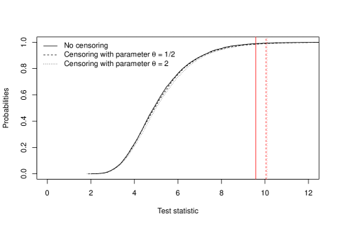
Figure 2. Empricial distribution function of the test statistic. The three $0.99$-quantiles are marked by the corresponding vertical lines.

The modified Cauchy model that we use for our simulation is one of the difficult models. It represents a typical model for which only the tail of the observed data (beyond the threshold $\tau$) is of type "heavy tailed", while the "beginning" and the "middle" (the part before the threshold $\tau$) of the distribution is not. In our case the part before the threshold $\tau$ can be of any form and is estimated non-parametrically (by the non-parametric Nelson-Aalen estimator). The tail is detected by our threshold selection procedure formulated in Section 4.

We compare the estimator defined by (2.8) with the usual non-parametric Nelson-Aalen estimator. Moreover, we have also compared both of them with the estimators described in (5.1) and (5.2). The number of aggregation is set by simulations to $M=40$ in the procedure described in Section 5.1 and 5.2.

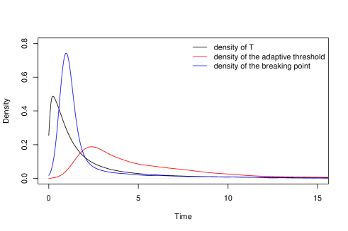
Figure 3. Density of the threshold $\widehat{\tau}$, the breaking point $\widehat{s}$ and the observations $T$ computed on $10000$ simulations of the transformed Cauchy distribution with parameters $x_{0}=0$ and $\gamma=1$.

In order to illustrate the choice of the transformed Cauchy distribution with location $x_{0}=0$ and scale $\gamma=1$, we show in Figure 3 the density of the failure time $X$, the density of the threshold $\widehat{\tau}$ and the breaking point $\widehat{s}$ chosen by the adaptive procedure presented in Section 4. One can see that the breaking point is chosen after the location parameter of the transformed Cauchy distribution and the threshold is therefore set to a value greater than it.

$n=100$
$x$	$100$	$200$	$300$	$400$	$500$
RelMSE of $\widehat{S}_{0}(x)$	4.6750	7.8920	10.2147	12.0651	13.6145
RelMSE of $\widehat{S}_{0,\widehat{\tau},\beta}(x)$	1.5908	2.1641	2.5413	2.8277	3.0605
RelMSE with simple aggregation	1.0306	1.4164	1.6714	1.8654	2.0234
RelMSE with adaptive aggregation	1.2361	1.6976	2.0023	2.2341	2.4229
$n=500$
$x$	$100$	$200$	$300$	$400$	$500$
RelMSE of $\widehat{S}_{0}(x)$	2.0733	4.1024	5.7537	7.1133	8.2953
RelMSE of $\widehat{S}_{0,\widehat{\tau},\beta}(x)$	0.4209	0.5844	0.6928	0.7754	0.8427
RelMSE with simple aggregation	0.4149	0.5771	0.6846	0.7666	0.8335
RelMSE with adaptive aggregation	0.3763	0.5253	0.6244	0.6999	0.7616

Table 1. $1000$ Monte-Carlo simulations where the parameters of the censorship distribution are $x_{0}=0$ and $\gamma=2$.

Assume that we have decided on the sample size $n$, the parameter $\beta$, the covariate distribution of $Z$, the baseline survival function $S_{0}(\cdot)$ and the censoring distribution $S_{C}(\left.\cdot\,\middle|\,z\right.)$. We generated data sets in our simulation study following the pattern : we consider $F_{0}$ to follow the transformed Cauchy distribution with parameters $x_{0}=0$ and $\gamma=1$. In the first study, the survival distribution function $S_{C}$ is assumed following the Cauchy distribution with parameter $x_{0}=0$ and $\gamma=2$. In a second study, $S_{C}$ is assumed following the transformed Cauchy distribution with parameter $x_{0}=10$ and $\gamma=0.1$. In both cases, the censoring survival distribution function doesn’t depend on the covariates. The mean censoring rate is around $50\%$ for the first distribution of $S_{C}$ and around $20\%$ for the second distribution of $S_{C}$.

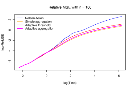
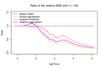
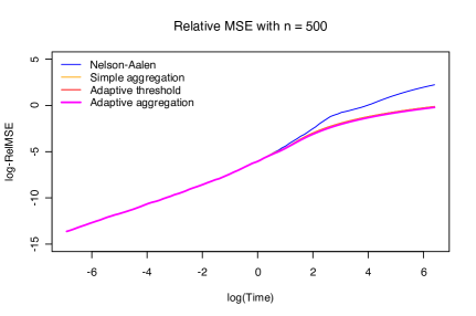
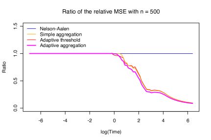
Figure 4. Relative MSE (left) and ratio of the relative MSE (right) for $n=100$ (top) and $n=500$ (bottom) and $NMC=1000$. The parameters of the censorship distribution are $x_{0}=0$ and $\gamma=2$.

The covariate is supposed to be a random uniform variable in $[-1,1]$ and the parameter $\beta$ is set to $-0.5$. For both $n=100$ and $n=500$, we chose $M=10$ thresholds for the aggregation procedure (simple and adaptive). For the simple aggregation, we chose $m_{0}$ corresponding to approximately $6\%$ of the observed values.

Table 1 gives the results of a Monte-Carlo simulation for the estimation of the baseline function with $S_{C}$ following a transformed Cauchy distribution with parameters $x_{0}=0$ and $\gamma=2$.

$n=100$
$x$	$100$	$200$	$300$	$400$	$500$
RelMSE of $\widehat{S}_{0}(x)$	5.1196	8.6637	11.1824	13.1688	14.8236
RelMSE of $\widehat{S}_{0,\widehat{\tau},\beta}(x)$	0.9857	1.3812	1.6447	1.8460	2.0104
RelMSE with simple aggregation	0.7266	1.0534	1.2749	1.4456	1.5857
RelMSE with adaptive aggregation	0.5970	0.8203	0.9681	1.0807	1.1725
$n=500$
$x$	$100$	$200$	$300$	$400$	$500$
RelMSE of $\widehat{S}_{0}(x)$	4.4576	7.7855	10.1777	12.0743	13.6595
RelMSE of $\widehat{S}_{0,\widehat{\tau},\beta}(x)$	0.2162	0.3128	0.3780	0.4281	0.4691
RelMSE with simple aggregation	0.4499	0.7033	0.8787	1.0154	1.1283
RelMSE with adaptive aggregation	0.1597	0.2257	0.2698	0.3036	0.3313

Table 2. $1000$ Monte-Carlo simulations with the following parameters of the censorship distribution $x_{0}=10$ and $\gamma=0.1$.

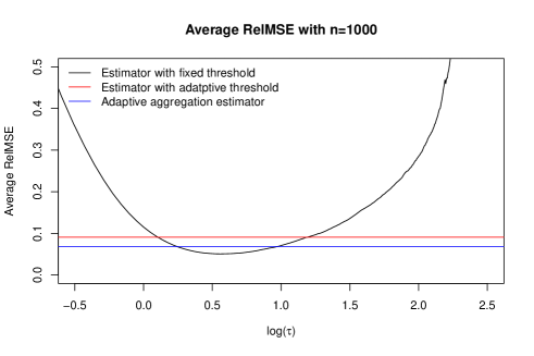
Figure 5. Average RelMSE’s of the estimator with fixed threshold $\tau$ (black line), of the estimator with the adaptive choice of the threshold (red line) and of the adaptively aggregated estimator (blue line). All estimators are computed on $10000$ simulations of the transformed Cauchy distribution with parameters $x_{0}=0$ and $\gamma=1$ and with parameters $x_{0}=0$ and $\gamma=2$ for the censorship .

Table 2 gives the results of a Monte-Carlo simulation for the estimation of the baseline function with $S_{C}$ following a transformed Cauchy distribution with parameters $x_{0}=10$ and $\gamma=0.1$. The performance of the adaptive choice of the threshold is shown on Figure 5. We plot the average RelMSE of the estimated survival function (2.8) with fixed threshold $\tau$, where $\tau$ is running on the uniform grid on $[0.1,20]$ (black line) and the average RelMSE of the estimated survival function (2.8) with the adaptive threshold $\widehat{\tau}$ (red line) chosen by the procedure described in Section 4. The average RelMSE is defined by : $ARelMSE_{\widehat{S_{0}}}=1/n_{grid}\sum_{j=1}^{n_{grid}}RelMSE_{\widehat{S_{0}}(x_{j})}$, where $x_{j},j=1,...,n_{grid}$ is a geometric grid on $[0.1,100]$. The average RelMSE of the aggregated estimated survival function $\widehat{S}_{0,\mbox{\scriptsize aa}}$ is also shown in blue line. One can see that the adaptive choice of the threshold is not optimal but it is close to the best one. Recall that the choice of the adaptive threshold is done without any prior knowledge of the ’best’ choice of the threshold (which sometimes is also called ’oracle’ choice).

We have added another model based on the $\log$-Gamma law, which has a rather "bad" slowly varying part of type $\log x$. The results are reported in Figure 6 and Table 3. These results show that the introduction of the aggregated estimator improves the estimation of the tails significantly with respect to standard Nelson-Aalen estimator. In particular, for low sample sizes, the aggregation improves the error estimation over the simple adaptive choice. The simulated distribution of the survival and censoring time follow a log-gamma distribution where the density function is defined for $x>1$ by:

$$f(x)=\frac{b^{a}\ln(x)^{a-1}}{\Gamma(a)x^{b+1}},$$

where $a>0$ is the shape parameter, $b>0$ is the rate parameter and $\Gamma(x)=\int_{0}^{\infty}t^{x-1}\exp(-t)dt$ is the Gamma function. We considered $F_{0}$ to follow a log-Gamma distribution with parameters $a=2$ and $b=2$ and $S_{C}$ to follow a log-Gamma distribution with parameters $a=5$ and $b=3.5$. The mean censoring rate is around $60\%$.

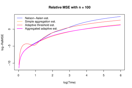
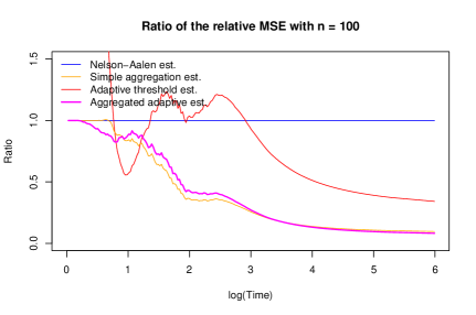
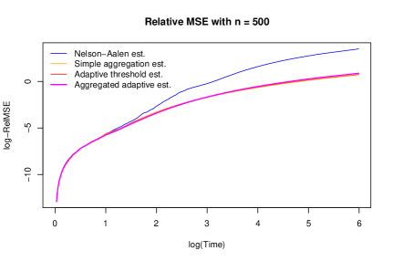
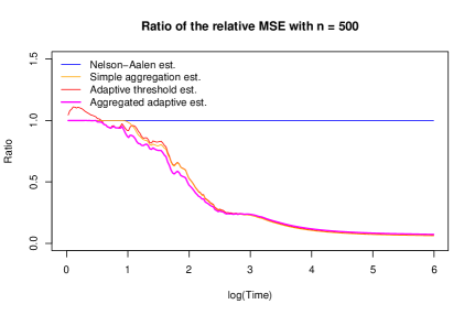
Figure 6. Relative MSE (left) and ratio of the relative MSE (right) for $n=100$ (top) and $n=500$ (bottom) and $NMC=1000$. The censorship follows a log-Gamma distribution with $a=5$ and $b=3.5$.

Figure 6 shows the $RelMSE$ and the ratio of $RelMSE$ of the baseline function compared to the Nelson-Aalen estimator where the baseline function follows a log-Gamma distribution with parameters $a=2$ and $b=2$. In Table 3, we compared the $RelMSE$ of estimated survival probabilites for extremes values.

$n=100$
$x$	$100$	$200$	$300$	$400$	$500$
RelMSE of $\widehat{S}_{0}(x)$	3.7469	7.6762	15.7922	27.1767	41.9159
RelMSE of $\widehat{S}_{0,\widehat{\tau},\beta}(x)$	2.5996	4.0775	6.7142	10.1159	14.3147
RelMSE with simple aggregation	0.7026	1.0984	1.8291	2.8042	4.0424
RelMSE with adaptive aggregation	0.7087	1.0536	1.6645	2.4551	3.4391
$n=500$
$x$	$100$	$200$	$300$	$400$	$500$
RelMSE of $\widehat{S}_{0}(x)$	1.7343	4.3083	10.5811	20.0979	32.9481
RelMSE of $\widehat{S}_{0,\widehat{\tau},\beta}(x)$	0.2985	0.4961	0.8774	1.4057	2.0957
RelMSE with simple aggregation	0.2876	0.4771	0.8439	1.3538	2.0217
RelMSE with adaptive aggregation	0.3110	0.5347	0.9744	1.5906	2.4005

Table 3. $1000$ Monte-Carlo simulations with the censorship distribution following a log-Gamma distribution with $a=5$ and $b=3.5$.

7. Applications

7.1. Bladder data set

As a second example, we consider the data set bladder included in the R package survival (https://cran.r-project.org/web/packages/survival/index.html). This data set concerns the comparison of different treatments on the recurrence of Stage I bladder tumor (see [29] for more details). We study here only the difference between the placebo and the thiotepa treatment. The initial purpose behind the study of this data set was to determine if the treatment had an effect on the recurrence of the bladder tumor. This study has been done in [30] using the usual Cox model. We want to extend the problem by determining the probability of having the first recurrence of the bladder tumor (the first recurrence is the most important to examine the treatment effect) at the end of the study for the placebo and treatment groups or at what time does the estimated probability of having the first recurrence fall below $0.3$.

We consider the observed time as the time between two recurrences or between the last recurrence and the censoring time. The covariate includes the treatment, the number of initial tumors, the size of the initial tumor and the number of recurrences.

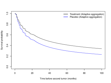
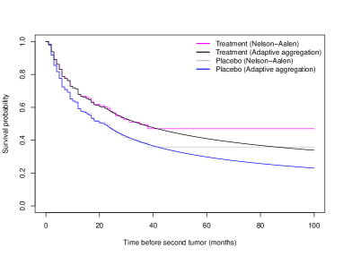
Figure 7. Estimated survival probabilities of the time of having the first recurrence of the bladder tumor when the initial size of the tumor is 1 and the initial number of tumors is 1.

One can see on the Figure 7 that our model fits the tail of the distribution and the recurrence time is estimated after the last observed time. The estimated survival probability of having the first recurrence of the tumor beyond 3 and 4 years are given in the following table.

Time (months)	$72$	$96$
Nelson-Aalen estimator (Placebo)	$0.3586$	$0.3586$
Nelson-Aalen estimator (Treatment)	$0.4697$	$0.4697$
Adaptive aggregation estimator (Placebo)	$0.2715$	$0.2348$
Adaptive aggregation estimator (Treatment)	$0.3826$	$0.3438$

Table 4. Estimated probabilities of having the first recurrence of the tumor beyond 3 and 4 years when the initial size of the tumor is 1, the initial number of tumors is 1.

The next table gives the estimated time at which a patient has a survival probability of having a first recurrence of $0.3$ and $0.4$.

Survival probability	$0.3$	$0.4$
Nelson-Aalen estimator (Placebo)	$NA$	$35$
Nelson-Aalen estimator (Treatment)	$NA$	$NA$
Adaptive aggregation estimator (Placebo)	$95.6232$	$43.3311$
Adaptive aggregation estimator (Treatment)	$194.9080$	$66.58699$

Table 5. Estimated time (months) of having the first recurrence of the tumor with a survival probabilities of $0.3$ and $0.4$ when the initial size of the tumor is 1, the initial number of tumors is 1.

One can see that with the model proposed in this paper, the initial problem of analyzing the estimated regression parameter to observe an effect of the treatment has been extended. It is possible to give an estimated probability of having the recurrence before a certain time and it’s possible to give an estimated time of recurrence for a given probability.

7.2. Application to electric consumption prediction

In order to offer an alternative to load shedding in case of an electric constraint, a research project has been conducted in Lorient, France, to study the electric consumption of households. The idea is to allocate the available electricity among all the consumers in the concerned area by lowering their usual power and so, avoiding the black out. This action can be done remotely from the smart meter. One of the objectives of the experiment is to study the behaviour of the consumers and the consequences on their consumption. Of course, the process will be used only when the market offers can not cope anymore. This action is known as ’active power modulation’. The data are collected on selected houses to study the effect during the electric constraint. For example, if a house with a maximal electric power contract of $9$ kiloVolt Ampere has a constraint of $50\%$, the maximal electric power becomes $4.5$ kVA. The goal of this study is to minimise the number of houses without electricity during a major power outages. If the electric power requested by the house exceeds the maximal permitted power, the breaker cuts off and the house has no electricity. In this section, we predict the electric power level for one random house during the time of the constraint and compare the measured level with what really happened.

The data used in this application are the electric power of a house with a maximal power contract of $9$ kVA. A measurement of the electric power is made every 10 minutes and corresponds to the mean load power requested in 10 minutes. The outside temperature is collected at the same times. The study period started on the $23$rd December, 2015 and finished on the $21$st March, 2016. Figure 8 shows the consumption of the studied house during the period and the measured outside temperature.

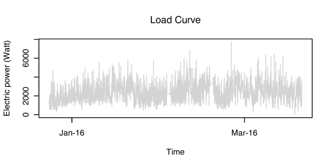
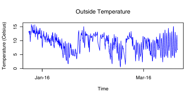
Figure 8. Load curve (top) and outside temperature (bottom) for the studied period.

As one can see in the Figure 8, we deal with a time series. We decided to remove the dependence of the time by discretized the data by hour, under the hypothesis that during the winter, the distribution of the electric power during the same hours remains similar over the days. The hours become part of the covariate and a binary information is given, e.g. a measurement between $2$h et $3$h will have a $1$ in during this hour and $0$ elsewhere.

Moreover, the temperature is included in the covariate with a subtle transformation. Indeed, we separated the temperature into $4$ linear covariates as we assume that the parameter of the temperature will not be constant over the scope of the temperature.

For this data set, the cumulative hazard rate functions are not proportionals. We decided to separate the data into five classes to improve the estimation of extreme probabilities. For each group corresponds a period during the day. The hour classes are from $22$h until $6$h which corresponds to the night. From $6$h until $10$h, which corresponds to the morning. From $10$h until $14$h, which corresponds to the lunch time. From $14$h until $18$h, which corresponds to the afternoon and finally from $18$h until $22$h, which corresponds to the evening.

The proportional hazards assumption almost holds for each groups. We are interested in the impact of the temperature onto this assumption, but the size of the data is not big enough to verify this.

Using the hypothesis from which the distribution of the electric power during the same hours is similar over the days during the winter, we estimate the survival functions. The goal is to predict the probability to exceed the maximal authorized power during the time of the constraint. Table 6 shows the different time of the constraint, the value of the maximal power during the constraint and the average outside temperature during the period starting the $23$rd December, 2015 and finishing the $21$st March, 2016. Recall that the maximal power of this house when there is no constraint is $9$ kVA. For each constraint, we give the estimated survival probability to exceed the maximal power given the time and the outside temperature.

Constraint day $11$th January $13$th January $18$th January $25$th February Constraint hours $17$-$19$h $14$-$18$h $14$-$18$h $14$-$18$h Maximal power $6.3$ kVA $4.5$ kVA $4.5$ kVA $4.5$ kVA Outside temperature $8.56$ T°C $8.85$ T°C $6.82$ T°C $9.85$ T°C Estimated survival $0.0015$ $0.09$ $0.1188$ $0.0778$ probability Number of cut off $0$ $0$ $0$ $0$ of the breaker Constraint day $1$st March $7$th March $18$th March Constraint hours $17$-$19$h $14$-$18$h $10$-$12$h Maximal power $3.6$ kVA $2.8$ kVA $2.8$ kVA Outside temperature $10.92$ T°C $9.70$ T°C $9.98$ T°C Estimated survival $0.0526$ $0.5018$ $0.7101$ probability Number of cut off $1$ $2$ $8$ of the breaker

Table 6. Date of the electric constraint, maximal power, outside temperature and estimated survival probabilities during the electric constraint. The number of cut off of the breaker represents the number of time the breaker cut off during the constraint period.

The probability corresponding to a return period of $4$ hours (happen once in any given $4$ hours period) is $\frac{1}{24}\simeq 0.04$. For a return period of $2$ hours, the corresponding probability is $0.08$. We can see on Table 6 that we detect five estimated probabilities exceeding the probability associated to the return period. These probabilities correspond to the constraints of the $13$th of January, the $18$th of January, the $15$th of February, the $7$th of March and the $18$th of March. This house is therefore considered at risk during these five constraints.

We are now interested to see what really happened for this house during these constraints. This house had one opening of its breaker during the constraint of the $1$st of March, two during the constraint of the $7$th of March, eight during the constraint of the $18$th of March and none during the other constraints. We can see that we have very high estimated probabilities of having one observation exceeding the maximal power during constraint for the $7$th and $18$th of March and that the house had multiple cuts off during these constraints. We can suppose that during the other constraints, the house anticipated the constraint period and reduced its electric power by changing its behavior.

8. Conclusion

In this article, we propose an extension of the Cox model in order to estimate probabilities of rare events and extreme quantiles. The model is semi-parametric and composed of the Nelson-Aalen estimator for the non-parametric part and the parametric part is described by a Pareto distribution. We prove the consistency of the estimator of the Pareto parameter and give an explicit convergence rate for the Hall model.

A data-driven choice of the threshold motivated by a goodness-of-fit test is proposed. An aggregated estimator and an adaptive aggregated estimator are suggested and studied in order to improve the fitness of the model onto the data. The performance of the proposed estimators is demonstrated on artificial data.

Two applications on real data sets are given. The application on the bladder data shows the motive of the model as it allows an estimation of extreme quantiles which was not possible with the usual Cox model. The application on the electric consumption gives an application onto data where the main purpose is to estimate survival probabilities and we are not interested to test if there is an effect of a treatment.

Appendix A Proofs of the results.

A.1. Proof of Theorem 2.1.

In the sequel we denote quasi-log-likelihood ratio by

$$\mathcal{L}(\left.\theta^{\prime},\theta\,\middle|\,\mathbf{z}\right.):=\mathcal{L}(\left.\theta^{\prime}\,\middle|\,\mathbf{z}\right.)-\mathcal{L}(\left.\theta\,\middle|\,\mathbf{z}\right.)=\sum_{i=1}^{n}\ln\frac{dP_{S_{0,\tau,\theta^{\prime}}}}{dP_{S_{0,\tau,\theta}}}\left(\left.t_{i},\delta_{i}\,\middle|\,z_{i}\right.\right).$$

Recall that we denoted by $\mathbb{P}$ the probability measure corresponding to the "true" model which has the baseline survival function $S_{0}$.

Lemma A.1.

For any $\theta,\theta^{\prime}\in\mathbb{R}$, $\mathbf{z}\in\mathbb{Z}$ and any $x>0$, it holds

$$\mathbb{P}(\mathcal{L}(\left.\theta^{\prime},\theta\,\middle|\,\mathbf{z}\right.)>x+\sum_{i=1}^{n}\chi^{2}(P_{S_{0}}(\left..\,\middle|\,z_{i}\right.),P_{S_{0,\tau,\theta}}(\left..\,\middle|\,z_{i}\right.)))\leq e^{-x/2}$$

Proof.

Let $P_{S_{0,\tau,\theta^{\prime}}}(\left..\,\middle|\,z_{i}\right.)$ and $P_{S_{0,\tau,\theta}}(\left..\,\middle|\,z_{i}\right.)$ be the conditional cumulative distribution function of $(T,\Delta)$ given $Z=z_{i}$ where the survival function has a Pareto tail with parameter $\theta^{\prime}$ and $\theta$ respectively for a threshold $\tau$. By Chebychev’s exponential inequality, we have for any $y>0$:

$$\mathbb{P}\left(\mathcal{L}(\left.\theta^{\prime},\theta\,\middle|\,\mathbf{z}\right.)>y\right) \leq e^{-y/2}\mathbb{E}\left(e^{\frac{1}{2}\mathcal{L}(\left.\theta^{\prime},\theta\,\middle|\,\mathbf{z}\right.)}\right)$$

$$\leq\exp\left[-y/2+\ln\left(\mathbb{E}\left(e^{\frac{1}{2}\mathcal{L}(\left.\theta^{\prime},\theta\,\middle|\,\mathbf{z}\right.)}\right)\right)\right].$$

As the triplet $\{\left.t_{1},\delta_{1}\,\middle|\,z_{1}\right.\},...,\{\left.t_{n},\delta_{n}\,\middle|\,z_{n}\right.\}$ are independent, we can write the term $\ln\left(\mathbb{E}\left(e^{\frac{1}{2}\mathcal{L}(\left.\theta^{\prime},\theta\,\middle|\,\mathbf{z}\right.)}\right)\right)$ as

$$\ln\left(\mathbb{E}\left(e^{\frac{1}{2}\mathcal{L}(\left.\theta^{\prime},\theta\,\middle|\,\mathbf{z}\right.)}\right)\right) =\ln\left(\mathbb{E}\left(e^{\frac{1}{2}\sum_{i=1}^{n}\ln\frac{dP_{S_{0,\tau,\theta^{\prime}}}}{dP_{S_{0,\tau,\theta}}}\left(\left.t_{i},\delta_{i}\,\middle|\,z_{i}\right.\right)}\right)\right)$$

$$=\ln\left(\mathbb{E}\left(\prod_{i=1}^{n}\sqrt{\frac{dP_{S_{0,\tau,\theta^{\prime}}}}{dP_{S_{0,\tau,\theta}}}\left(\left.t_{i},\delta_{i}\,\middle|\,z_{i}\right.\right)}\right)\right)$$

$$=\sum_{i=1}^{n}\ln\left(\mathbb{E}\left(\sqrt{\frac{dP_{S_{0,\tau,\theta^{\prime}}}}{dP_{S_{0,\tau,\theta}}}\left(\left.t_{i},\delta_{i}\,\middle|\,z_{i}\right.\right)}\right)\right).$$

By Hölder’s inequality, we have

$$\mathbb{E}\left(\sqrt{\frac{dP_{S_{0,\tau,\theta^{\prime}}}}{dP_{S_{0,\tau,\theta}}}\left(\left.t_{i},\delta_{i}\,\middle|\,z_{i}\right.\right)}\right) \leq\sqrt{\mathbb{E}\left(\frac{dP_{S_{0,\tau,\theta^{\prime}}}}{dP_{S_{0,\tau,\theta}}}\left(\left.t_{i},\delta_{i}\,\middle|\,z_{i}\right.\right)\right)}$$

$$\leq\sqrt{1+\chi^{2}(P_{S_{0}}\left(\left.\cdot\,\middle|\,z_{i}\right.\right),P_{S_{0,\tau,\theta}}\left(\left.\cdot\,\middle|\,z_{i}\right.\right))},$$

where the $\chi^{2}$ entropy between two equivalent probability measure is defined by (2.11). Then,

$$\mathbb{P}\left(\mathcal{L}(\left.\theta^{\prime},\theta\,\middle|\,\mathbf{z}\right.)>y\right) \leq\exp\left[-\frac{y}{2}+\frac{1}{2}\sum_{i=1}^{n}\ln\left(1+\chi^{2}(P_{S_{0}}\left(\left.\cdot\,\middle|\,z_{i}\right.\right),P_{S_{0,\tau,\theta}}\left(\left.\cdot\,\middle|\,z_{i}\right.\right))\right)\right]$$

$$\leq\exp\left[-\frac{y}{2}+\frac{1}{2}\sum_{i=1}^{n}\chi^{2}(P_{S_{0}}\left(\left.\cdot\,\middle|\,z_{i}\right.\right),P_{S_{0,\tau,\theta}}\left(\left.\cdot\,\middle|\,z_{i}\right.\right))\right].$$

Setting $y=x+\sum_{i=1}^{n}\chi^{2}(P_{S_{0}}\left(\left.\cdot\,\middle|\,z_{i}\right.\right),P_{S_{0,\tau,\theta}}\left(\left.\cdot\,\middle|\,z_{i}\right.\right))$, gives Lemma A.1. ∎

Recall that the Kullback-Leibler divergence $\mathcal{K}(\theta^{\prime},\theta)$ between two Pareto distribution with parameters $\theta^{\prime}$ and $\theta$ is defined by (2.10). The following lemma gives the rate of convergence for $\widehat{\theta}_{\tau}$. We adapt the proof from [20] to the case of the Cox model under consideration in this paper.

Lemma A.2.

For any $\theta>0$, $\tau>x_{0}$ and $v>0$, it holds

$$\mathbb{P}\left(\widehat{n}_{\tau}\mathcal{K}(\widehat{\theta}_{\tau},\theta)>v+\sum_{i=1}^{n}\chi^{2}(P_{S_{0}}\left(\left.\cdot\,\middle|\,z_{i}\right.\right),P_{S_{0,\tau,\theta}}\left(\left.\cdot\,\middle|\,z_{i}\right.\right))+2\ln(n)\right)\leq 2\exp(-v/2),$$

where $\widehat{n}_{\tau}=\sum_{t_{i}>\tau}\delta_{i}$.

Proof.

It is easy to see that the assertion of lemma follows from the following bound:

(A.1) $$\mathbb{P}\left(\widehat{n}_{\tau}\mathcal{K}(\widehat{\theta}_{\tau},\theta)>v+\sum_{i=1}^{n}\chi^{2}(P_{S_{0}}\left(\left.\cdot\,\middle|\,z_{i}\right.\right),P_{S_{0,\tau,\theta}}\left(\left.\cdot\,\middle|\,z_{i}\right.\right))\right)\leq 2n\exp\left(-\frac{v}{2}\right).$$

The likelihood ratio is given by

(A.2) $$\mathcal{L}(\left.\theta^{\prime},\theta\,\middle|\,\mathbf{z}\right.) :=\mathcal{L}(\left.\theta^{\prime}\,\middle|\,\mathbf{z}\right.)-\mathcal{L}(\left.\theta\,\middle|\,\mathbf{z}\right.)$$

$$=\sum_{i=1}^{n}\ln p_{S_{0,\tau,\theta^{\prime}}}(\left.t_{i},\delta_{i}\,\middle|\,z_{i}\right.)-\sum_{i=1}^{n}\ln p_{S_{0,\tau,\theta}}(\left.t_{i},\delta_{i}\,\middle|\,z_{i}\right.).$$

Then, removing the censoring part from the likelihood ratio, we have

$$\mathcal{L}(\left.\theta^{\prime},\theta\,\middle|\,\mathbf{z}\right.) =\sum_{i=1}^{n}\ln(h_{z_{i},\tau,\theta^{\prime}}(t_{i})^{\delta_{i}}S_{{z_{i},\tau,\theta^{\prime}}}(t_{i}))-\sum_{i=1}^{n}\ln(h_{{z_{i},\tau,\theta}}(t_{i})^{\delta_{i}}S_{{z_{,}\tau,\theta}}(t_{i}))$$

$$=\sum_{i=1}^{n}\delta_{i}\ln(h_{0,\tau,\theta^{\prime}}(t_{i})e^{\beta\cdot z_{i}})+\ln(S_{z_{i},\tau,\theta^{\prime}}(t_{i}))$$

$$-\delta_{i}\ln(h_{0,\tau,\theta}(t_{i})e^{\beta\cdot z_{i}})-\ln(S_{z_{i},\tau,\theta}(\left.t_{i}\,\middle|\,z_{i}\right.))).$$

Developing the terms, we obtain

$$\mathcal{L}(\left.\theta^{\prime},\theta\,\middle|\,\mathbf{z}\right.) =\sum_{i=1}^{n}\delta_{i}\ln(h_{0}(t_{i}))\mathbb{1}_{t_{i}\leq\tau}+\delta_{i}\ln(\frac{1}{\theta^{\prime}t_{i}})\mathbb{1}_{t_{i}>\tau}+\delta_{i}\beta\cdot z_{i}$$

$$\qquad\qquad\qquad\qquad\qquad\qquad\qquad\qquad+e^{\beta\cdot z_{i}}\ln(S_{0,\tau,\theta^{\prime}}(t_{i}))$$

$$-\delta_{i}\ln(h_{0}(t_{i}))\mathbb{1}_{t_{i}\leq\tau}-\delta_{i}\ln(\frac{1}{\theta t_{i}})\mathbb{1}_{t_{i}>\tau}-\delta_{i}\beta\cdot z_{i}-e^{\beta\cdot z_{i}}\ln(S_{0,\tau,\theta}(t_{i})),$$

and further

$$\mathcal{L}(\left.\theta^{\prime},\theta\,\middle|\,\mathbf{z}\right.) =\sum_{i=1}^{n}\left[\delta_{i}\ln\left(\frac{\theta}{\theta^{\prime}}\right)-e^{\beta\cdot z_{i}}\frac{1}{\theta^{\prime}}\ln\left(\frac{t_{i}}{\tau}\right)+e^{\beta\cdot z_{i}}\frac{1}{\theta}\ln\left(\frac{t_{i}}{\tau}\right)\right]\mathbb{1}_{t_{i}>\tau}$$

$$=\sum_{i=1}^{n}\left[\delta_{i}\ln\left(\frac{\theta}{\theta^{\prime}}\right)+e^{\beta\cdot z_{i}}\ln\left(\frac{t_{i}}{\tau}\right)\left(\frac{1}{\theta}-\frac{1}{\theta^{\prime}}\right)\right]\mathbb{1}_{t_{i}>\tau}.$$

Since

$$\widehat{\theta}_{\tau}=\frac{\sum_{i:t_{i}>\tau}e^{\beta\cdot z_{i}\ln\left(\frac{t_{i}}{\tau}\right)}}{\sum_{i:t_{i}>\tau}\delta_{i}},$$

using (A.2), it follows that

$$\mathcal{L}(\left.\theta^{\prime},\theta\,\middle|\,\mathbf{z}\right.) :=\mathcal{L}(\left.\theta^{\prime}\,\middle|\,\mathbf{z}\right.)-\mathcal{L}(\left.\theta\,\middle|\,\mathbf{z}\right.)$$

$$=\sum_{i=1}^{n}\mathbb{1}_{t_{i}>\tau}\delta_{i}\ln\left(\frac{\theta}{\theta^{\prime}}\right)+\sum_{i=1}^{n}\mathbb{1}_{t_{i}>\tau}\delta_{i}\widehat{\theta}_{\tau}\left(\frac{1}{\theta}-\frac{1}{\theta^{\prime}}\right)$$

$$=\sum_{i=1}^{n}\mathbb{1}_{t_{i}>\tau}\delta_{i}\left[\ln\left(\frac{\theta}{\theta^{\prime}}\right)+\widehat{\theta}_{\tau}\left(\frac{1}{\theta}-\frac{1}{\theta^{\prime}}\right)\right]$$

$$=\widehat{n}_{\tau}\left(\ln\left(\frac{\theta}{\theta^{\prime}}\right)+\left(\frac{1}{\theta}-\frac{1}{\theta^{\prime}}\right)\widehat{\theta}_{\tau}\right)$$

(A.3) $$=\widehat{n}_{\tau}\Lambda(\theta^{\prime}),$$

where we denoted for brevity $\Lambda(\theta^{\prime})=\ln\left(\frac{\theta}{\theta^{\prime}}\right)-\left(\frac{1}{\theta^{\prime}}-\frac{1}{\theta}\right)\widehat{\theta}_{\tau}$. Since $\mathcal{K}(\theta^{\prime},\theta)=\frac{\theta^{\prime}}{\theta}-1-\ln(\frac{\theta^{\prime}}{\theta})$, we then have the identity

(A.4) $$\mathcal{K}(\widehat{\theta}_{\tau},\theta)=\Lambda(\widehat{\theta}_{\tau}).$$

Using (A.3) and (A.4) we hope to bound $\mathcal{K}(\widehat{\theta}_{\tau},\theta)$ in probability by Lemma A.1. The problem is that $\widehat{\theta}_{\tau}$ is random and therefore we cannot apply Lemma A.1 directly. We shall circumvent this difficulty in the following way. For any $y>0$ and any $k\geq 1$, the inequality $k\mathcal{K}(u,\theta)>y$ can be equivalently written as

$$\left(\frac{1}{u}-\frac{1}{\theta}\right)\widehat{\theta}_{\tau} <-\frac{y}{k}+\ln\left(\frac{\theta}{u}\right).$$

Setting $g(u,k)=\frac{\ln\left(\frac{\theta}{u}\right)-\frac{y}{k}}{\left(\frac{1}{u}-\frac{1}{\theta}\right)}$, we have $g(u,k)>\widehat{\theta}_{\tau}$, when $0<u<\theta$ and $g(u,k)<\widehat{\theta}_{\tau}$, when $u>\theta$. Moreover, the function $g(u,k)$ has a maximum for $0<u<\theta$ and a minimum for $u>\theta$. When $0<u<\theta$, we have $\lim\limits_{u\rightarrow 0^{+}}\frac{dg(u,k)}{du}=+\infty$ and $\lim\limits_{u\rightarrow\theta^{-}}\frac{dg(u,k)}{du}=-\infty$. When $u>\theta$, we have $\lim\limits_{u\rightarrow\theta^{+}}\frac{dg(u,k)}{du}=+\infty$ and $\lim\limits_{u\rightarrow+\infty}\frac{dg(u,k)}{du}=0^{-}$. Let

$$\theta^{+}(k)=\underset{0<u<\theta}{\operatorname{{\mbox{argmax}}}}\ g(u,k)\ \ \text{and}\ \ \theta^{-}(k)=\underset{u>\theta}{\operatorname{\mbox{argmin}}}\ g(u,k),$$

then

$$\{\widehat{n}_{\tau}\Lambda(\widehat{\theta}_{\tau})>y,\widehat{\theta}_{\tau}<\theta\} =\{g(\widehat{\theta}_{\tau},\widehat{n}_{\tau})>\widehat{\theta}_{\tau},\widehat{\theta}_{\tau}<\theta\}$$

$$\subset\{g(\theta^{+}(\widehat{n}_{\tau}),\widehat{n}_{\tau})>\widehat{\theta}_{\tau},\widehat{\theta}_{\tau}<\theta\}$$

$$=\{\widehat{n}_{\tau}\Lambda(\theta^{+}(\widehat{n}_{\tau}))>y,\widehat{\theta}_{\tau}<\theta\}$$

$$\subset\{\widehat{n}_{\tau}\Lambda(\theta^{+}(\widehat{n}_{\tau}))>y\}.$$

In the same way, we have $\{\widehat{n}_{\tau}\Lambda(\widehat{\theta}_{\tau})>y,\widehat{\theta}_{\tau}>\theta\}\subset\{\widehat{n}_{\tau}\Lambda(\theta^{-}(\widehat{n}_{\tau}))>y\}$. Since $\mathcal{K}(\widehat{\theta}_{\tau},\theta)=\Lambda(\widehat{\theta}_{\tau})$, this implies

$$\{\widehat{n}_{\tau}\Lambda(\widehat{\theta}_{\tau})>y\}\subset\{\widehat{n}_{\tau}\Lambda(\theta^{+}(\widehat{n}_{\tau}))>y\}\cup\{\widehat{n}_{\tau}\Lambda(\theta^{-}(\widehat{n}_{\tau}))>y\}.$$

We then have

$$\mathbb{P}(\widehat{n}_{\tau}\mathcal{K}(\widehat{\theta}_{\tau},\theta)>y) \leq\mathbb{P}(\widehat{n}_{\tau}\Lambda(\theta^{+}(\widehat{n}_{\tau}))>y)+\mathbb{P}(\widehat{n}_{\tau}\Lambda(\theta^{-}(\widehat{n}_{\tau}))>y)$$

(A.5) $$\leq\sum_{k=1}^{n}\mathbb{P}(\widehat{n}_{\tau}\Lambda(\theta^{+}(k))>y)+\sum_{k=1}^{n}\mathbb{P}(\widehat{n}_{\tau}\Lambda(\theta^{-}(k))>y).$$

Now we can apply Lemma A.1, with

(A.6) $$y=v+\sum_{i=1}^{n}\chi^{2}(P_{S_{0}}\left(\left.\cdot\,\middle|\,z_{i}\right.\right),P_{S_{0,\tau,\theta}}\left(\left.\cdot\,\middle|\,z_{i}\right.\right))$$

from which it follows that, for $k=1,...,n$,

(A.7) $$\mathbb{P}(\widehat{n}_{\tau}\Lambda(\theta^{\pm}(k))>y)\leq e^{-v/2}.$$

From (A.5) and (A.7),

(A.8) $$\mathbb{P}(\widehat{n}_{\tau}\mathcal{K}(\widehat{\theta}_{\tau},\theta)>y)\leq 2ne^{-v/2}.$$

This and (A.6) yields (A.1), thus concluding the proof of Lemma A.2. ∎

Theorem 2.1 follows, if we set $v=2\ln(n)$ in Lemma A.2.

A.2. Verification of Condition 2

Lemma A.3.

Assume that the distribution functions given the covariate $z$ of both the survival and censoring time are in the maximal domain of attraction of the Fréchet law with parameters $\theta(z)$ and $\theta_{C}(z)$ respectively. Then, for any z,

$$q_{F}(\left.\tau\,\middle|\,z\right.)\to\frac{\theta(z)}{\theta_{C}(z)+\theta(z)}\ \text{as}\ \tau\to\infty.$$

where $\theta(z)>0$ and $\theta_{C}(z)>0$.

Proof.

We have for any z,

$$q_{F}(\left.\tau\,\middle|\,z\right.)=\int_{\tau}^{\infty}\frac{S(\left.t\,\middle|\,z\right.)}{S(\left.\tau\,\middle|\,z\right.)}\frac{f_{C}(\left.t\,\middle|\,z\right.)}{S_{C}(\left.\tau\,\middle|\,z\right.)}dt\in[0,1],\quad\tau\geq x_{0}.$$

Since $F$ and $F_{C}$ are in the maximal domain of attraction of the Fréchet law, for some $\theta(z)>0$ and $\theta_{C}(z)>0$, we have

$$\frac{S(\left.\tau t\,\middle|\,z\right.)}{S(\left.\tau\,\middle|\,z\right.)}\to t^{-1/\theta(z)},\ \text{as}\ \tau\to\infty,$$

and

$$\frac{S_{C}(\left.\tau t\,\middle|\,z\right.)}{S_{C}(\left.\tau\,\middle|\,z\right.)}\to t^{-1/\theta_{C}(z)},\ \text{as}\ \tau\to\infty.$$

Therefore,

$$\lim_{\tau\to\infty}q_{F}(\left.\tau\,\middle|\,z\right.)=\lim_{\tau\to\infty}\int_{\tau}^{\infty}\frac{S(\left.t\,\middle|\,z\right.)}{S(\left.\tau\,\middle|\,z\right.)}\frac{f_{C}(\left.t\,\middle|\,z\right.)}{S_{C}(\left.\tau\,\middle|\,z\right.)}dt.$$

By the Lebesgue theorem of dominated convergence,

$$\lim_{\tau\to\infty}q_{F}(\left.\tau\,\middle|\,z\right.) =\int_{1}^{\infty}t^{-1/\theta(z)}\frac{1}{\theta_{C}(z)\tau}t^{-1/\theta_{C}(z)-1}d\tau t$$

$$=\frac{1}{\theta_{C}(z)}\int_{1}^{\infty}t^{-\frac{\theta_{C}(z)+\theta(z)}{\theta(z)\theta_{C}(z)}-1}dt$$

$$=\frac{1}{\theta_{C}(z)}\frac{\theta(z)\theta_{C}(z)}{\theta_{C}(z)+\theta(z)}$$

$$=\frac{\theta(z)}{\theta_{C}(z)+\theta(z)}.$$

∎

A.3. Proof of Theorem 2.2

We begin with an auxiliary theorem.

Theorem A.4.

Assume condition (2) and (3). Then, there exists a constant $c>0$ such that,

$$\lim_{n\to\infty}\mathbb{P}\left(\mathcal{K}(\widehat{\theta}_{\tau},\theta)\leq c\frac{\sum_{i=1}^{n}\chi^{2}(P_{S_{0}}(\left..\,\middle|\,z_{i}\right.),P_{S_{0,\tau,\theta}}(\left..\,\middle|\,z_{i}\right.))+4\ln(n)}{\sum_{i=1}^{n}S_{C}(\left.\tau\,\middle|\,z_{i}\right.)S(\left.\tau\,\middle|\,z_{i}\right.)}\right)=1,$$

where $P_{S_{0}}(\left..\,\middle|\,z_{i}\right.)$ is the cumulative distribution function of (2.6) and $P_{S_{0,\tau,\theta}}(\left..\,\middle|\,z_{i}\right.)$ is the cumulative distribution function of the joint density of the model (2.3).

Proof.

Theorem A.4 follows from Theorem 2.1 and the following Lemma A.5. ∎

Lemma A.5.

Assume condition (2). Then, for every $\tau\geq x_{0}$,

$$\mathbb{E}(\widehat{n}_{\tau})\geq\sum_{i=1}^{n}S(\left.\tau\,\middle|\,z_{i}\right.)S_{C}(\left.\tau\,\middle|\,z_{i}\right.)(1-q_{0}),$$

and

$$\mathbb{P}(\widehat{n}_{\tau}\leq\mathbb{E}(\widehat{n}_{\tau})/2)\leq e^{-\mathbb{E}(\widehat{n}_{\tau})/8}.$$

Proof.

By the density of the model (2.6), we have

$$\mathbb{E}(\widehat{n}_{\tau})=\sum_{i=1}^{n}\int_{\tau}^{\infty}f(\left.x\,\middle|\,z_{i}\right.)S_{C}(\left.x\,\middle|\,z_{i}\right.)dx,$$

where $\widehat{n}_{\tau}=\sum_{t_{i}>\tau}\delta_{i}$. Therefore,

$$\mathbb{E}(\widehat{n}_{\tau}) =\sum_{i=1}^{n}\left(\left[-S(\left.x\,\middle|\,z_{i}\right.)S_{C}(\left.x\,\middle|\,z_{i}\right.)\right]_{\tau}^{\infty}-\int_{\tau}^{\infty}S(\left.x\,\middle|\,z_{i}\right.)f_{C}(\left.x\,\middle|\,z_{i}\right.)dx\right)$$

$$=\sum_{i=1}^{n}\left(S(\left.\tau\,\middle|\,z_{i}\right.)S_{C}(\left.\tau\,\middle|\,z_{i}\right.)-S(\left.\tau\,\middle|\,z_{i}\right.)S_{C}(\left.\tau\,\middle|\,z_{i}\right.)\int_{\tau}^{\infty}\frac{S(\left.x\,\middle|\,z_{i}\right.)}{S(\left.\tau\,\middle|\,z_{i}\right.)}\frac{f_{C}(\left.x\,\middle|\,z_{i}\right.)}{S_{C}(\left.\tau\,\middle|\,z_{i}\right.)}dx\right)$$

$$=\sum_{i=1}^{n}S(\left.\tau\,\middle|\,z_{i}\right.)S_{C}(\left.\tau\,\middle|\,z_{i}\right.)(1-q_{F}(\left.\tau\,\middle|\,z_{i}\right.)).$$

using $q_{F}(\left.\tau\,\middle|\,z_{i}\right.)\leq q_{0}$ for any $z_{i}$ proves the first part of the Lemma.

The second inequality follows from the exponential bound for binomial random variables, and is established by using standard techniques going back to Chernoff [31].

∎

Lemma A.6.

Assume that $Q$ and $Q_{0}$ are two equivalent probability measures on a measurable space. Then,

$$\chi^{2}(Q,Q_{0})\leq\int\left(\ln\frac{dQ}{dQ_{0}}\right)^{2}\exp\left|\frac{dQ}{dQ_{0}}\right|dQ.$$

Proof.

The proof can be found in the article [20]. ∎

Now we proceed to prove Theorem 2.2. We start by providing the following bound:

$$\max_{z\in\mathbb{Z}}\chi^{2}(P_{S_{0}}(\left.\cdot\,\middle|\,z\right.),P_{S_{0,\tau,\theta}}(\left.\cdot\,\middle|\,z\right.))\leq O_{\mathbb{P}}\left(\rho_{\tau}^{2}\max_{z\in\mathbb{Z}}S(\left.\tau\,\middle|\,z\right.)S_{C}(\left.\tau\,\middle|\,z\right.)\right).$$

By Lemma A.6, we have

$$\max_{z\in\mathbb{Z}}\chi^{2}(P_{S_{0}}(\left..\,\middle|\,z\right.),P_{S_{0,\tau,\theta}}(\left..\,\middle|\,z\right.))$$

$$\leq\max_{z\in\mathbb{Z}}\int\ln^{2}\frac{dP_{S_{0}}(\left.t,\delta\,\middle|\,z\right.)}{dP_{S_{0,\tau,\theta}}(\left.t,\delta\,\middle|\,z\right.)}\exp\left|\ln\frac{dP_{S_{0}}(\left.t,\delta\,\middle|\,z\right.)}{dP_{S_{0,\tau,\theta}}(\left.t,\delta\,\middle|\,z\right.)}\right|P_{S_{0}}(\left.dt,d\delta\,\middle|\,z\right.).$$

For any $x>\tau$, we have

$$\ln\frac{dP_{S_{0}}(\left.t,\delta\,\middle|\,z\right.)}{dP_{S_{0,\tau,\theta}}(\left.t,\delta\,\middle|\,z\right.)} =\ln\frac{h(\left.t\,\middle|\,z\right.)^{\delta}S(\left.t\,\middle|\,z\right.)}{h_{\theta}(\left.t\,\middle|\,z\right.)^{\delta}S_{\theta,\tau}(\left.t\,\middle|\,z\right.)}$$

$$=\ln\frac{h_{0}(t)^{\delta}(e^{\beta\cdot z})^{\delta}e^{-\int_{\tau}^{t}h_{0}(u)e^{\beta\cdot z}du}}{h_{0,\tau,\theta}(t)^{\delta}(e^{\beta\cdot z})^{\delta}e^{-\int_{\tau}^{t}h_{0,\tau,\theta}(u)e^{\beta\cdot z}du}}$$

$$=\delta\ln\frac{h_{0}(t)}{(\theta t)^{-1}}-e^{\beta\cdot z}\int_{\tau}^{t}(h_{0}(u)-\frac{1}{\theta u})du.$$

It follows

$$\left|\ln\frac{dP_{S_{0}}(\left.t,\delta\,\middle|\,z\right.)}{dP_{S_{0,\tau,\theta}}(\left.t,\delta\,\middle|\,z\right.)}\right| =\left|\delta\ln\frac{h_{0}(t)}{(\theta t)^{-1}}-\int_{\tau}^{t}\left(h(\left.u\,\middle|\,z\right.)-\frac{1}{\theta u}e^{\beta\cdot z}\right)du\right|$$

$$=\left|\delta\ln(\frac{th_{0}(t)}{\theta^{-1}}-1+1)-\int_{\tau}^{t}\left(uh(\left.u\,\middle|\,z\right.)-\frac{1}{\theta}e^{\beta\cdot z}\right)\frac{du}{u}\right|$$

$$\leq\delta 2\theta\left|th_{0}(t)-\frac{1}{\theta}\right|+\left|\int_{\tau}^{t}\left(uh(\left.u\,\middle|\,z\right.)-\frac{1}{\theta}e^{\beta\cdot z}\right)\frac{du}{u}\right|.$$

Let $\rho_{\tau}=\sup_{t>\tau}\left|th_{0}(t)-\frac{1}{\theta}\right|$, then

$$\left|\ln\frac{dP_{S_{0}}(\left.t,\delta\,\middle|\,z\right.)}{dP_{S_{0,\tau,\theta}}(\left.t,\delta\,\middle|\,z\right.)}\right|\leq\rho_{\tau}\left(\delta 2\theta+e^{\beta\cdot z}\ln\frac{t}{\tau}\right).$$

We have

$$\max_{z\in\mathbb{Z}}\chi^{2}(P_{S_{0}}(\left.\cdot\,\middle|\,z\right.),P_{S_{0,\tau,\theta}}(\left.\cdot\,\middle|\,z\right.))$$

$$\leq\max_{z\in\mathbb{Z}}\int\left(\ln\frac{dP_{S_{0}}(\left.\cdot\,\middle|\,z\right.)}{dP_{S_{0,\tau,\theta}}(\left.\cdot\,\middle|\,z\right.)}\right)^{2}\exp\left|\ln\frac{dP_{S_{0}}(\left.\cdot\,\middle|\,z\right.)}{dP_{S_{0,\tau,\theta}}(\left.\cdot\,\middle|\,z\right.)}\right|dP_{S_{0}}(\left.\cdot\,\middle|\,z\right.)$$

$$\leq\max_{z\in\mathbb{Z}}\int_{\tau}^{\infty}\sum_{\delta\in\{0,1\}}\rho_{\tau}^{2}\left(\delta 2\theta+e^{\beta\cdot z}\ln\frac{t}{\tau}\right)^{2}\exp(\rho_{\tau}\left(\delta 2\theta+e^{\beta\cdot z}\ln\frac{t}{\tau}\right))P_{S_{0}}(\left.t,\delta\,\middle|\,z\right.)dt$$

$$\leq\max_{z\in\mathbb{Z}}\int_{\tau}^{\infty}\rho_{\tau}^{2}e^{2\beta\cdot z}\ln^{2}\frac{t}{\tau}\exp\left(\rho_{\tau}e^{\beta\cdot z}\ln\frac{t}{\tau}\right)S(\left.t\,\middle|\,z\right.)f_{C}(\left.t\,\middle|\,z\right.)$$

$$+\rho_{\tau}^{2}\left(2\theta+e^{\beta\cdot z}\ln\frac{t}{\tau}\right)^{2}\exp\left(\rho_{\tau}(2\theta+e^{\beta\cdot z}\ln\frac{t}{\tau})\right)f(\left.t\,\middle|\,z\right.)S_{C}(\left.t\,\middle|\,z\right.)dt$$

$$\leq\max_{z\in\mathbb{Z}}\int_{\tau}^{\infty}\rho_{\tau}^{2}\left(\frac{t}{\tau}\right)^{\rho_{\tau}}\left(e^{2\beta\cdot z}\ln^{2}\frac{t}{\tau}+\left(2\theta+e^{\beta\cdot z}\ln\frac{t}{\tau}\right)^{2}e^{2\rho_{\tau}\theta}\right)$$

$$\qquad\qquad\qquad\qquad\times\left(f(\left.t\,\middle|\,z\right.)S_{C}(\left.t\,\middle|\,z\right.)+S(\left.t\,\middle|\,z\right.)f_{C}(\left.t\,\middle|\,z\right.)\right)dt.$$

Let $g(u)=\left(e^{2\beta\cdot z}u^{2}+(2\theta+e^{\beta\cdot z}u)^{2}e^{2\rho_{\tau}\theta}\right)e^{\rho_{\tau}u}$. Then

$$\max_{z\in\mathbb{Z}}\chi^{2}(P_{S_{0}}(\left..\,\middle|\,z\right.),P_{S_{0,\tau,\theta}}(\left..\,\middle|\,z\right.))$$

$$\leq\max_{z\in\mathbb{Z}}\int_{\tau}^{\infty}\rho_{\tau}^{2}g\left(\ln\frac{t}{\tau}\right)(f(\left.t\,\middle|\,z\right.)S_{C}(\left.t\,\middle|\,z\right.)+S(\left.t\,\middle|\,z\right.)f_{C}(\left.t\,\middle|\,z\right.))dt.$$

Since $S(\left.t\,\middle|\,z\right.)\leq S(\left.\tau\,\middle|\,z\right.)$ and $S_{C}(\left.t\,\middle|\,z\right.)\leq S_{C}(\left.\tau\,\middle|\,z\right.)$ for every $t>\tau$, we obtain

$$\max_{z\in\mathbb{Z}}\chi^{2}(P_{S_{0}}(\left..\,\middle|\,z\right.),P_{S_{0,\tau,\theta}}(\left..\,\middle|\,z\right.))$$

$$\leq\max_{z\in\mathbb{Z}}\rho_{\tau}^{2}\int_{\tau}^{\infty}g\left(\ln\frac{t}{\tau}\right)$$

$$\qquad\qquad\times\left(\frac{f(\left.t\,\middle|\,z\right.)}{S(\left.\tau\,\middle|\,z\right.)}S(\left.\tau\,\middle|\,z\right.)S_{C}(\left.\tau\,\middle|\,z\right.)+\frac{f_{C}(\left.t\,\middle|\,z\right.)}{S_{C}(\left.\tau\,\middle|\,z\right.)}S(\left.\tau\,\middle|\,z\right.)S_{C}(\left.\tau\,\middle|\,z\right.)\right)dt$$

$$\leq\max_{z\in\mathbb{Z}}\rho_{\tau}^{2}S(\left.\tau\,\middle|\,z\right.)S_{C}(\left.\tau\,\middle|\,z\right.)\int_{\tau}^{\infty}g\left(\ln\frac{t}{\tau}\right)\left(\frac{f(\left.t\,\middle|\,z\right.)}{S(\left.\tau\,\middle|\,z\right.)}+\frac{f_{C}(\left.t\,\middle|\,z\right.)}{S_{C}(\left.\tau\,\middle|\,z\right.)}\right)dt.$$

We can rewrite the ratio $\frac{S(\left.t\,\middle|\,z\right.)}{S(\left.\tau\,\middle|\,z\right.)}$ as $e^{-\int_{\tau}^{t}h(\left.u\,\middle|\,z\right.)du}=e^{-\int_{\tau}^{t}uh(\left.u\,\middle|\,z\right.)\frac{du}{u}}$. We know that $th(\left.t\,\middle|\,z\right.)$ is bounded below for $t$ large enough by : $th(\left.t\,\middle|\,z\right.)\geq\frac{e^{\beta\cdot z}}{2\theta}$. Then,

$$\frac{S(\left.t\,\middle|\,z\right.)}{S(\left.\tau\,\middle|\,z\right.)}\leq e^{-\frac{e^{\beta\cdot z}}{2\theta}\ln\frac{t}{\tau}}.$$

We know that :

$$\frac{d}{dt}g\left(\ln\frac{t}{\tau}\right) =\frac{d}{dt}\left(\ln^{2}\frac{t}{\tau}+\left(2\theta+\ln\frac{t}{\tau}\right)^{2}e^{2\rho_{\tau}\theta}\right)e^{\rho_{\tau}\ln\frac{t}{\tau}}$$

$$=\left[\frac{2}{t}\ln\frac{t}{\tau}+e^{2\rho_{\tau}\theta}\frac{2}{t}\left(2\theta+\ln\frac{t}{\tau}\right)\right]e^{\rho_{\tau}\ln\frac{t}{\tau}}$$

$$+\left(\ln^{2}\frac{t}{\tau}+\left(2\theta+\ln\frac{t}{\tau}\right)^{2}e^{2\rho_{\tau}\theta}\right)e^{\rho_{\tau}\ln\frac{t}{\tau}}\rho_{\tau}\frac{1}{t}$$

$$=\left(\frac{t}{\tau}\right)^{\rho_{\tau}-1}\Bigg{[}\frac{2}{\tau}\ln\frac{t}{\tau}+\frac{2}{\tau}e^{2\rho_{\tau}\theta}2\theta+\frac{2}{\tau}e^{2\rho_{\tau}\theta}\ln\frac{t}{\tau}+\frac{\rho_{\tau}}{\tau}\ln^{2}\frac{t}{\tau}$$

$$\qquad+\frac{\rho_{\tau}}{\tau}4\theta^{2}e^{2\rho_{\tau}\theta}+\frac{\rho_{\tau}}{\tau}4\theta\ln\frac{t}{\tau}e^{2\rho_{\tau}\theta}+\frac{\rho_{\tau}}{\tau}\ln^{2}\frac{t}{\tau}e^{2\rho_{\tau}\theta}\Bigg{]}.$$

Integrating by parts the term $\int_{\tau}^{\infty}g\left(\ln\frac{t}{\tau}\right)\left(\frac{f(\left.t\,\middle|\,z\right.)}{S(\left.\tau\,\middle|\,z\right.)}\right)dt$, we have :

$$\int_{\tau}^{\infty}g\left(\ln\frac{t}{\tau}\right)\frac{f(\left.t\,\middle|\,z\right.)}{S(\left.\tau\,\middle|\,z\right.)}dt$$

$$=\left[-g\left(\ln\frac{t}{\tau}\right)\frac{S(\left.t\,\middle|\,z\right.)}{S(\left.\tau\,\middle|\,z\right.)}\right]^{\infty}_{\tau}+\int_{\tau}^{\infty}\frac{S(\left.t\,\middle|\,z\right.)}{S(\left.\tau\,\middle|\,z\right.)}g^{\prime}\left(\ln\frac{t}{\tau}\right)dx$$

$$\leq 4\theta^{2}e^{2\rho_{\tau}\theta}+\int_{\tau}^{\infty}e^{-\frac{e^{\beta\cdot z}}{2\theta}\ln\frac{t}{\tau}}g^{\prime}(\ln\frac{t}{\tau})dt$$

$$\leq 4\theta^{2}e^{2\rho_{\tau}\theta}+\int_{\tau}^{\infty}\left(\frac{t}{\tau}\right)^{\rho_{\tau}-\frac{e^{\beta\cdot z}}{2\theta}-1}\cdot\Bigg{[}\frac{2}{\tau}\ln\frac{t}{\tau}+\frac{2}{\tau}e^{2\rho_{\tau}\theta}2\theta+\frac{2}{\tau}e^{2\rho_{\tau}\theta}\ln\frac{t}{\tau}$$

$$\qquad\qquad\qquad+\frac{\rho_{\tau}}{\tau}\ln^{2}\frac{t}{\tau}+\frac{\rho_{\tau}}{\tau}4\theta^{2}e^{2\rho_{\tau}\theta}+\frac{\rho_{\tau}}{\tau}4\theta\ln\frac{t}{\tau}e^{2\rho_{\tau}\theta}+\frac{\rho_{\tau}}{\tau}\ln^{2}\frac{t}{\tau}e^{2\rho_{\tau}\theta}\Bigg{]}dt.$$

We know that $\rho_{\tau}$ is supposed to be small for large values of $t$. It is safe to say that $t^{\rho_{\tau}-\frac{e^{\beta\cdot z}}{2\theta}-1}\leq t^{-\frac{1}{4\theta}}$. Then, $\int_{\tau}^{\infty}g\left(\ln\frac{t}{\tau}\right)\frac{f(\left.t\,\middle|\,z\right.)}{S(\left.\tau\,\middle|\,z\right.)}dt$ can be bounded by a constant.

$$\int_{\tau}^{\infty}g\left(\ln\frac{t}{\tau}\right)\frac{f(\left.t\,\middle|\,z\right.)}{S(\left.\tau\,\middle|\,z\right.)}dt=O_{\mathbb{P}}(1).$$

In the same way, for $h_{C}(\left.t\,\middle|\,z\right.)\geq c^{\prime\prime}$, for $t\geq\tau$, we have

$$\int_{\tau}^{\infty}g\left(\ln\frac{t}{\tau}\right)\frac{f_{C}(\left.t\,\middle|\,z\right.)}{S_{C}(\left.t\,\middle|\,z\right.)}dt=O_{\mathbb{P}}(1).$$

Then:

$$\max_{z\in\mathbb{Z}}\chi^{2}(P_{S_{0}}(\left.\cdot\,\middle|\,z\right.),P_{S_{0,\tau,\theta}}(\left.\cdot\,\middle|\,z\right.))\leq O_{\mathbb{P}}\left(\rho_{\tau}^{2}\max_{z\in\mathbb{Z}}S(\left.\tau\,\middle|\,z\right.)S_{C}(\left.\tau\,\middle|\,z\right.)\right).$$

Using the previous bound with $\tau=\tau_{n}$, we have, as $n\rightarrow\infty$,

(A.9) $$\sum_{i=1}^{n}\chi^{2}(P_{S_{0}}(\left.\cdot\,\middle|\,z_{i}\right.),P_{S_{0,\tau_{n},\theta}}(\left.\cdot\,\middle|\,z_{i}\right.))\leq n\rho_{\tau_{n}}^{2}\max_{z\in\mathbb{Z}}S(\left.\tau_{n}\,\middle|\,z\right.)S_{C}(\left.\tau_{n}\,\middle|\,z\right.)\rightarrow 0,$$

since $\max_{z\in\mathbb{Z}}S(\left.\tau_{n}\,\middle|\,z\right.)S_{C}(\left.\tau_{n}\,\middle|\,z\right.)\leq 1$ and by condition (2.13),

$$n\rho_{\tau_{n}}^{2}\rightarrow 0\quad\text{as}\quad n\rightarrow\infty.$$

On the other hand, from condition (2.14), we have

$$\sum_{i=1}^{n}S_{C}(\left.\tau_{n}\,\middle|\,z_{i}\right.)S(\left.\tau_{n}\,\middle|\,z_{i}\right.)\rightarrow\infty\quad\text{as}\quad n\rightarrow\infty.$$

Since, by Theorem A.4, we have:

$$\lim_{n\to\infty}\mathbb{P}\left(\mathcal{K}(\widehat{\theta}_{\tau_{n}},\theta)\leq c\frac{\sum_{i=1}^{n}\chi^{2}(P_{S_{0}}(\left.\cdot\,\middle|\,z_{i}\right.),P_{S_{0,\tau_{n},\theta}}(\left.\cdot\,\middle|\,z_{i}\right.))+4\ln(n)}{\sum_{i=1}^{n}S_{C}(\left.\tau_{n}\,\middle|\,z_{i}\right.)S(\left.\tau_{n}\,\middle|\,z_{i}\right.)}\right)=1,$$

using (2.10), it is easy to see that $\mathcal{K}(\widehat{\theta}_{\tau_{n}},\theta)\rightarrow 0$ as $n\rightarrow\infty$, which means that

$$\widehat{\theta}_{\tau_{n}}\xrightarrow[n\rightarrow\infty]{\mathbb{P}}\theta.$$

A.4. Proof of Theorem 3.1

Proof.

Starting from the auxiliary result in the proof for the Theorem 2.2, we have

$$\max_{z\in\mathbb{Z}}\chi^{2}(P_{S_{0}}(\left.\cdot\,\middle|\,z\right.),P_{S_{0,\tau,\theta}}(\left.\cdot\,\middle|\,z\right.))\leq O_{\mathbb{P}}\left(\rho_{\tau}^{2}\max_{z\in\mathbb{Z}}S(\left.\tau\,\middle|\,z\right.)S_{C}(\left.\tau\,\middle|\,z\right.)\right)\quad\text{as }\tau\rightarrow\infty.$$

We now want to find a sequence of threshold $(\tau_{n})$ such that

$$\max_{z\in\mathbb{Z}}S(\left.\tau_{n}\,\middle|\,z\right.)S_{C}(\left.\tau_{n}\,\middle|\,z\right.)\rho_{\tau_{n}}^{2}\leq c_{0}\left(\frac{\ln n}{n}\right).$$

Suppose that there exists a sequence of $(\tau_{n})$ and a constant $c_{0}$ such that

(A.10) $$\max_{z\in\mathbb{Z}}\chi^{2}(P_{S_{0}}(\left..\,\middle|\,z\right.),P_{S_{0,\tau_{n},\theta_{\tau_{n}}}}(\left..\,\middle|\,z\right.))=c_{0}\frac{\ln n}{n}.$$

Since the baseline hazard function is assumed to satisfy (5), we have,

$$|xh(\left.x\,\middle|\,z\right.)-\frac{1}{\theta}e^{\beta\cdot z}|\leq c_{1}^{\prime}x^{-\frac{\alpha e^{\beta\cdot z}}{\theta}}.$$

From (5), we find the following lower bound for $xh(\left.x\,\middle|\,z\right.)$:

$$xh(\left.x\,\middle|\,z\right.) \geq\frac{e^{\beta\cdot z}}{\theta}-|xh(\left.x\,\middle|\,z\right.)-\frac{e^{\beta\cdot z}}{\theta}|$$

$$\geq\frac{e^{\beta\cdot z}}{\theta}-c_{1}x^{-\frac{\alpha e^{\beta\cdot z}}{\theta}}.$$

We note that

$$\max_{z\in\mathbb{Z}}S(\left.\tau_{n}\,\middle|\,z\right.) =\max_{z\in\mathbb{Z}}\exp\left(-\int_{x_{0}}^{\tau_{n}}h(\left.t\,\middle|\,z\right.)dt\right)$$

$$=\max_{z\in\mathbb{Z}}\exp\left(-\int_{x_{0}}^{\tau_{n}}th(\left.t\,\middle|\,z\right.)\frac{dt}{t}\right)$$

$$\leq\max_{z\in\mathbb{Z}}\exp\left(-\frac{e^{\beta\cdot z}}{\theta}\ln\frac{\tau_{n}}{x_{0}}-\frac{\theta c_{1}^{\prime}}{\alpha e^{\beta\cdot z}}\left(\tau_{n}^{-\frac{\alpha e^{\beta\cdot z}}{\theta}}-x_{0}^{-\frac{\alpha e^{\beta\cdot z}}{\theta}}\right)\right)$$

$$\leq\max_{z\in\mathbb{Z}}\exp\left(-\frac{e^{\beta\cdot z}}{\theta}\ln\frac{\tau_{n}}{x_{0}}\right)\exp\left(\frac{c_{1}^{\prime}}{\alpha}x_{0}^{-\alpha}\right).$$

We now find bounds for $xh_{C}(\left.x\,\middle|\,z\right.)$.

$$xh_{C}(\left.x\,\middle|\,z\right.)-\frac{\gamma e^{\beta\cdot z}}{\theta} \geq-|xh_{C}(\left.x\,\middle|\,z\right.)-\frac{\gamma e^{\beta\cdot z}}{\theta}|$$

$$xh_{C}(\left.x\,\middle|\,z\right.) \geq\frac{\gamma e^{\beta\cdot z}}{\theta}-|xh_{C}(\left.x\,\middle|\,z\right.)-\frac{\gamma e^{\beta\cdot z}}{\theta}|$$

$$\geq\frac{\gamma e^{\beta\cdot z}}{\theta}-c_{2}x^{-\mu}.$$

We have

$$\max_{z\in\mathbb{Z}}S_{C}(\left.\tau_{n}\,\middle|\,z\right.) =\max_{z\in\mathbb{Z}}\exp\left(-\int_{x_{0}}^{\tau_{n}}h_{C}(\left.x\,\middle|\,z\right.)dx\right)$$

$$=\max_{z\in\mathbb{Z}}\exp\left(-\int_{x_{0}}^{\tau_{n}}xh_{C}(\left.x\,\middle|\,z\right.)\frac{dx}{x}\right)$$

$$\leq\max_{z\in\mathbb{Z}}\exp\left(-\frac{\gamma e^{\beta\cdot z}}{\theta}\ln\frac{\tau_{n}}{x_{0}}-\frac{c_{2}}{\mu}\left(\tau_{n}^{-\mu}-x_{0}^{-\mu}\right)\right)$$

$$\leq\max_{z\in\mathbb{Z}}\exp\left(-\frac{\gamma e^{\beta\cdot z}}{\theta}\ln\frac{\tau_{n}}{x_{0}}\right)\exp\left(\frac{c_{2}}{\mu}x_{0}^{-\mu}\right).$$

Then,

(A.11) $$\max_{z\in\mathbb{Z}}S(\left.\tau_{n}\,\middle|\,z\right.)S_{C}(\left.\tau_{n}\,\middle|\,z\right.)\rho_{\tau_{n}}^{2}\leq\max_{z\in\mathbb{Z}}(c_{1}^{\prime})^{2}\tau_{n}^{-(\frac{e^{\beta\cdot z}}{\theta}+\frac{\gamma e^{\beta\cdot z}}{\theta}+2\frac{\alpha e^{\beta\cdot z}}{\theta})}x_{0}^{\frac{e^{\beta\cdot z}}{\theta}+\frac{\gamma e^{\beta\cdot z}}{\theta}}c_{3}.$$

Solving the equation (A.11) for $\tau_{n}$ yields

$$\max_{z\in\mathbb{Z}}(c_{1}^{\prime})^{2}\tau_{n}^{-(\frac{e^{\beta\cdot z}}{\theta}+\frac{\gamma e^{\beta\cdot z}}{\theta}+2\frac{\alpha e^{\beta\cdot z}}{\theta})}x_{0}^{\frac{e^{\beta\cdot z}}{\theta}+\frac{\gamma e^{\beta\cdot z}}{\theta}}c_{3}=c_{0}\left(\frac{\ln n}{n}\right),$$

$$\tau_{n}=n^{\frac{\theta}{\underset{z\in\mathbb{Z}}{\min}(e^{\beta\cdot z})(1+\gamma+2\alpha)}}\ln^{-\frac{\theta}{\underset{z\in\mathbb{Z}}{\min}(e^{\beta\cdot z})(1+\gamma+2\alpha)}}n,$$

$$\tau_{n}=n^{\frac{\nicefrac{{\theta}}{{\underset{z\in\mathbb{Z}}{\min}(e^{\beta\cdot z})}}}{1+\gamma+2\alpha}}\ln^{-\frac{\nicefrac{{\theta}}{{\underset{z\in\mathbb{Z}}{\min}(e^{\beta\cdot z})}}}{1+\gamma+2\alpha}}n.$$

Now, we search a lower bound for $\sum_{i=1}^{n}S_{(}\left.\tau\,\middle|\,z_{i}\right.)S_{C}(\left.\tau_{n}\,\middle|\,z_{i}\right.)$. We have for any $z$,

$$S(\left.\tau_{n}\,\middle|\,z\right.) =\exp\left(-\int_{x_{0}}^{\tau_{n}}th(\left.t\,\middle|\,z\right.)\frac{dt}{t}\right)$$

$$\geq\exp\left(-\frac{e^{\beta\cdot z}}{\theta}\ln\frac{\tau_{n}}{x_{0}}-\frac{\theta c_{1}}{-\alpha e^{\beta\cdot z}}\left(\tau_{n}^{-\frac{\alpha e^{\beta\cdot z}}{\theta}}-x_{0}^{-\frac{\alpha e^{\beta\cdot z}}{\theta}}\right)\right)$$

$$\geq\exp\left(-\frac{e^{\beta\cdot z}}{\theta}\ln\frac{\tau_{n}}{x_{0}}\right)\exp\left(-\frac{\theta c_{1}^{\prime}}{\alpha e^{\beta\cdot z}}x_{0}^{-\frac{\alpha e^{\beta\cdot z}}{\theta}}\right),$$

and

$$S_{C}(\left.\tau_{n}\,\middle|\,z\right.) =\exp\left(-\int_{x_{0}}^{\tau_{n}}xh_{C}(x)\frac{dx}{x}\right)$$

$$\geq\exp\left(-\frac{\gamma e^{\beta\cdot z}}{\theta}\ln\frac{\tau_{n}}{x_{0}}\right)\exp\left(-\frac{c_{2}}{\mu}x_{0}^{-\mu}\right).$$

Choosing $z$ such as minimizing $\sum_{i=1}^{n}S_{(}\left.\tau\,\middle|\,z_{i}\right.)S_{C}(\left.\tau_{n}\,\middle|\,z_{i}\right.)$ yields the result of the theorem. ∎

References

- [1] Cox DR. Regression models and life-tables. Journal of the Royal Statistical Society Series B (Methodological). 1972;34(2):187–220. Available from: http://www.jstor.org/stable/2985181.
- [2] Fleming TR, Harrington DP. Counting processes and survival analysis. Vol. 169. John Wiley & Sons; 2011.
- [3] Andersen PK, Borgan O, Gill RD, et al. Statistical models based on counting processes. Springer Science & Business Media; 2012.
- [4] Therneau TM, Grambsch PM. Modeling survival data: extending the Cox model. Springer Science & Business Media; 2013.
- [5] Klein JP, Moeschberger ML. Survival analysis: techniques for censored and truncated data. Springer Science & Business Media; 2005.
- [6] Crowley J, Hu M. Covariance analysis of heart transplant survival data. Journal of the American Statistical Association. 1977;72(357):27–36.
- [7] Lee EW, Wei LJ, Amato DA, et al. Cox-type regression analysis for large numbers of small groups of correlated failure time observations. In: Survival analysis: state of the art. Springer; 1992. p. 237–247.
- [8] Embrechts P, Klüppelberg C, Mikosch T. Modelling extremal events: for insurance and finance. Vol. 33. Springer Science & Business Media; 2013.
- [9] McNeil AJ. Estimating the tails of loss severity distributions using extreme value theory. ASTIN bulletin. 1997;27(01):117–137.
- [10] Danielsson J, de Vries CG. Tail index and quantile estimation with very high frequency data. Journal of empirical Finance. 1997;4(2):241–257.
- [11] Gardes L, Girard S. Conditional extremes from heavy-tailed distributions: an application to the estimation of extreme rainfall return levels. Extremes. 2010;13:177–204.
- [12] Durrieu G, Grama I, Pham Q, et al. Nonparametric adaptive estimator of extreme conditional tail probabilities quantiles. Extremes. 2015;18:437–478.
- [13] Beirlant J, Guillou A, Dierckx G, et al. Estimation of the extreme value index and extreme quantiles under random censoring. Extremes. 2007;10(3):151–174.
- [14] Beirlant J, Guillou A, Toulemonde G. Peaks-over-threshold modeling under random censoring. Communications in Statistics?Theory and Methods. 2010;39(7):1158–1179.
- [15] Einmahl JH, Fils-Villetard A, Guillou A, et al. Statistics of extremes under random censoring. Bernoulli. 2008;14(1):207–227.
- [16] Stupfler G. Estimating the conditional extreme-value index under random right-censoring. Journal of Multivariate Analysis. 2016;144:1–24.
- [17] Ndao P, Diop A, Dupuy JF. Nonparametric estimation of the conditional tail index and extreme quantiles under random censoring. Computational Statistics & Data Analysis. 2014;79:63–79.
- [18] Ndao P, Diop A, Dupuy JF. Nonparametric estimation of the conditional extreme-value index with random covariates and censoring. Journal of Statistical Planning and Inference. 2016;168:20–37.
- [19] Grama I, Spokoiny V. Statistics of extremes by oracle estimation. Annals of Statistics. 2008;36(4):1619–1648.
- [20] Grama I, Tricot JM, Petiot JF. Estimation of the extreme survival probabilities from censored data. Buletinul Academiei de Stiinte a Repunlicii Moldova Matematica. 2014;74(1):33–62.
- [21] Beirlant J, Goegebeur Y, Teugels J, et al. Statistics of extremes: Theory and applications. John Wiley & Sons; 2004.
- [22] Hill BM, et al. A simple general approach to inference about the tail of a distribution. The Annals of Statistics. 1975;3(5):1163–1174.
- [23] Nelson W. Theory and applications of hazard plotting for censored failure data. Technometrics. 1972;14(4):945–966.
- [24] Aalen O. Nonparametric inference for a family of counting processes. The Annals of Statistics. 1978;:701–726.
- [25] Breslow NE. Discussion of professor Cox’s paper. J Royal Stat Soc B. 1972;34:216–217.
- [26] Hall P. On some simple estimates of an exponent of regular variation. Journal of the Royal Statistical Society Series B (Methodological). 1982;:37–42.
- [27] Hall P, Welsh AH. Best attainable rates of convergence for estimates of parameters of regular variation. The Annals of Statistics. 1984;:1079–1084.
- [28] Drees H. Optimal rates of convergence for estimates of the extreme value index. Annals of Statistics. 1998;:434–448.
- [29] Byar DP. The veterans administration study of chemoprophylaxis for recurrent stage i bladder tumours: comparisons of placebo, pyridoxine and topical thiotepa. In: Bladder tumors and other topics in urological oncology. Springer; 1980. p. 363–370.
- [30] Wei LJ, Lin DY, Weissfeld L. Regression analysis of multivariate incomplete failure time data by modeling marginal distributions. Journal of the American statistical association. 1989;84(408):1065–1073.
- [31] Chernoff H, et al. A measure of asymptotic efficiency for tests of a hypothesis based on the sum of observations. The Annals of Mathematical Statistics. 1952;23(4):493–507.