Mass and shape of the Milky Way’s dark matter halo with globular clusters from Gaia and Hubble

Abstract

Aims. We estimate the mass of the inner ($<20$ kpc) Milky Way and the axis ratio of its inner dark matter halo using globular clusters as tracers. At the same time, we constrain the distribution in phase-space of the globular cluster system around the Galaxy.

Methods. We use the Gaia Data Release 2 catalogue of 75 globular clusters’ proper motions and recent measurements of the proper motions of another 20 distant clusters obtained with the Hubble Space Telescope. We describe the globular cluster system with a distribution function (DF) with two components: a flat, rotating disc-like one and a rounder, more extended halo-like one. While fixing the Milky Way’s disc and bulge, we let the mass and shape of the dark matter halo and we fit these two parameters, together with six others describing the DF, with a Bayesian method.

Results. We find the mass of the Galaxy within 20 kpc to be $M(<20{\,\rm kpc})=1.91^{+0.18}_{-0.17}\times 10^{11}M_{\odot}$, of which $M_{\rm DM}(<20{\,\rm kpc})=1.37^{+0.18}_{-0.17}\times 10^{11}M_{\odot}$ is in dark matter, and the density axis ratio of the dark matter halo to be $q=1.30\pm 0.25$. Assuming a concentration-mass relation, this implies a virial mass $M_{\rm vir}=1.3\pm 0.3\times 10^{12}M_{\odot}$. Our analysis rules out oblate ($q<0.8$) and strongly prolate halos ($q>1.9$) with 99% probability. Our preferred model reproduces well the observed phase-space distribution of globular clusters and has a disc component that closely resembles that of the Galactic thick disc. The halo component follows a power-law density profile $\rho\propto r^{-3.3}$, has a mean rotational velocity of $V_{\rm rot}\simeq-14\,\rm km\,s^{-1}$ at 20 kpc, and has a mildly radially biased velocity distribution ($\beta\simeq 0.2\pm 0.07$, which varies significantly with radius only within the inner 15 kpc). We also find that our distinction between disc and halo clusters resembles, although not fully, the observed distinction in metal-rich ([Fe/H]$>-0.8$) and metal-poor ([Fe/H]$\leq-0.8$) cluster populations.

1 Introduction

Giant leaps in the physical understanding of our Universe are often made when new superb datasets that peer into previously uncharted territory become available. The second data release of Gaia (Gaia Collaboration et al. 2018a) has just arrived and is by all means a perfect instance of such a leap. The extent, accuracy, and quality of the data provided is unprecedented, and it is leading the field of Galactic Astronomy to a completely new era.

While most of the new discoveries and exciting results are probably still hidden in the vastness of the dataset, the increase in the number of objects observed and the greater accuracy, for example of the measured tangential motions on the sky, has the potential to immediately lead to ground-breaking results (Gaia Collaboration et al. 2018b, c; Antoja et al. 2018). In this study we exploit this novel dataset by employing a well-established, but very sophisticated method to infer new tight constraints on fundamental parameters, such as the total mass and the shape of the gravitational potential of the inner Milky Way.

We do this by using the catalogue of absolute proper motions that Gaia Collaboration et al. (2018b) estimated for 75 globular clusters (GCs) around the Milky Way. Thanks to the unprecedented performances of the Gaia astrometry, proper motions for these satellites could be measured with a typical accuracy of a few tens of $\rm\mu as\,yr^{-1}$, which roughly corresponds to an accuracy of $0.5-2\rm\,km\,s^{-1}$ in tangential velocity for a cluster located at 10 kpc from us. Remarkable measurements of similar accuracy were also recently released by Sohn et al. (2018) using the Hubble Space Telescope (HST). These authors estimated proper motions of 20 clusters at large Galactocentric distances ($>10$ kpc), using two HST epochs at least $\sim 6$ yr apart.

With the dataset provided by these two new catalogues, we can use the GCs as tracers of the Galactic potential and hope to infer its total mass (e.g. Bahcall & Tremaine 1981; Watkins, Evans, & An 2010). Moreover, given the size and the unprecedented accuracy of the new catalogue, there may well be enough signal in the data to constrain simultaneously the mass and the axis ratio of the isodensity surfaces of the total mass distribution of the Galaxy, similarly to previous work using the kinematics of individual stars in the Milky Way halo (e.g. Olling & Merrifield 2000; Smith, Wyn Evans, & An 2009; Bowden, Evans, & Williams 2016; Posti et al. 2018). In order to have enough inference from the data, we can model the Milky Way GC system with equilibrium models in an arbitrary axisymmetric Galactic potential. One possibility is then to use distribution functions (DFs) to represent the phase-space distribution of the GC system and to measure the characteristic parameters of such DFs with the data from Gaia and HST. This would not only allow the determination of the fundamental parameters of the Galactic potential, but would also simultaneously constrain the full phase-space distribution of the GCs around the Milky Way.

In this paper we use this approach and follow closely Binney & Wong (2017, hereafter BW17), who described the GC system with two distinct DFs, one with halo-like dynamics (typically representing the metal-poor clusters), and one with disc-like dynamics (following the more metal-rich clusters, see Zinn 1985). These DFs are constructed in the space of the action integrals of motion. We build upon the work of BW17 and improve on it in several ways: i) we use a much larger and more accurate dataset provided by very recent measurements presented above, ii) we allow for the dark matter halo mass and shape to vary in our fit, and iii) we simplify the description of the DFs by fixing some characteristic parameters while still reproducing remarkably well the observed distribution of GCs.

The paper is organised as follows: we introduce the data used in Section 2 and our modelling technique in Section 3; we describe our Bayesian approach to determine the distribution of the model parameters in Section 4 and we discuss our results in Section 5; finally, we summarise and conclude in Section 6. Throughout the paper we use a distance to the Galactic centre of $R_{\odot}=8.3$ kpc and a peculiar motion of the Sun of $(U_{\odot},V_{\odot},W_{\odot})=(11.1,12.24,7.25)\rm\,km\,s^{-1}$ (Schönrich, Binney, & Dehnen 2010). We note, however, that reasonable differences in $R_{\odot}$ and in the solar peculiar motion (see §3.2 and §5.3.3 in Bland-Hawthorn & Gerhard 2016, respectively) are too small to significantly affect our conclusions.

2 Data

2.1 Globular cluster data from Gaia DR2 and the Hubble Space Telescope

Our dataset is primarily composed of the recently estimated proper motions and radial velocities for 75 GCs from the Gaia Collaboration et al. (2018b). This catalogue provides data of the best quality which is ideal to study the motion in phase-space of GCs with unprecedented accuracy. The following observables are provided: $(\alpha,\delta)$ are right ascension and declination, and $(\mu_{\alpha*},\mu_{\delta})$ are the respective proper motions on the sky. Alongside these measurements, we also have standard uncertainties and the correlation between the two proper motions $C_{\mu_{\alpha*},\mu_{\delta}}$, which we use for generating samples from the error distribution of each cluster. We supplement the Gaia DR2 catalogue with the recent measurements of 16 other GCs from Sohn et al. (2018). Hence, we work with an unprecedented total of 91 GCs with exquisite proper motion data quality.

For both sets of clusters we compute heliocentric distances $s$ from the extinction-corrected distance moduli in the $V$-band, taken from the latest version of the catalogue compiled by Harris (1996), and we assume the uncertainty to be $0.05$ mag for each object. The heliocentric radial velocities $v_{\rm rad}$ and their uncertainties are also taken from this catalogue. Therefore, the set of observables that we use is

$${\bf w}=(\alpha,\delta,s,\mu_{\alpha*},\mu_{\delta},v_{\rm rad}),$$ (1)

where the error distribution of each cluster is assumed to be a multi-variate normal distribution with non-null correlation $C_{\mu_{\alpha*},\mu_{\delta}}$ between the proper motions and negligible variances in the sky positions $(\alpha,\delta)$ for the Gaia DR2 clusters. We also add an additional systematic 35 $\rm\mu as\,yr^{-1}$ to the uncertainty budget of the cluster proper motion measured by Gaia, as advised in Gaia Collaboration et al. (2018b).

Finally, to make our tracer sample as complete as possible, we also consider 52 GCs for which no proper motion data is available. For this sample, we again obtain distance moduli and radial velocities, together with their uncertainties from Harris (1996). This leaves us with a total sample of $91+52=143$ GCs.

2.2 Sagittarius clusters

Several of the known GCs have been tentatively associated with the Sagittarius dwarf galaxy/stream by different authors in the past (see e.g. Law & Majewski 2010). The Sagittarius dwarf galaxy is currently merging with our Galaxy (Ibata, Gilmore, & Irwin 1994) and it is possibly bringing in a few GCs. If a significant fraction of the GCs that we use as tracers are actually associated with the dwarf galaxy, this would imply a non-random sampling of Galactic phase-space which could lead to biased estimates of the mass and shape of the Galactic potential using our DF-based method.

For this reason we run our algorithm with the full sample of GCs, but also excluding the four clusters Arp 2, Palomar 12, Terzan 7, and Terzan 8 that have been associated with the Sagittarius dwarf galaxy according to the dynamical analysis of Law & Majewski (2010) and have been recently confirmed by Sohn et al. (2018). We retain M 54, the nuclear cluster in Sagittarius, as this now traces the orbit of the dwarf singly. In addition, we also remove from our analysis NGC 5053, which was recently found to be one of a pair of clusters (with NGC5024, Gaia Collaboration et al. 2018b).

3 Dynamical model

Here we introduce the technique that we use to model the distribution in phase space of the GC population given a Galactic gravitational potential. Our method borrows heavily from BW17, to which we refer the reader to for a more exhaustive description. The Galactic potentials, the mapping from position-velocities $({\bf x},{\bf v})$ to action-angles $(\boldsymbol{\theta},{\bf J})$ and the DF models are constructed with the AGAMA code (Vasiliev 2018).

Table 1: Fixed parameters of the model (see also Piffl et al. 2014b)

Galactic Potential Parameters
	Thin disc	Thick disc	Gas disc
$\Sigma_{0}/M_{\odot}\,{\rm pc}^{2}$	$570.7$	$251.0$	$94.5$
$R_{\rm d}/{\rm kpc}$	$2.7$	$2.7$	$5.4$
$h_{\rm d}/{\rm kpc}$	$0.2$	$0.7$	$0.04$
$R_{\rm hole}/{\rm kpc}$	$0$	$0$	$4$
	Bulge
$\rho_{0}/M_{\odot}\,{\rm kpc}^{3}$	$9.5\times 10^{10}$
$q$	$0.5$
$a$	$0$
$b$	$1.8$
$r_{0}/{\rm kpc}$	$0.075$
$r_{\rm cut}/{\rm kpc}$	$2.1$
Distribution Function Parameters
$R_{\sigma}/{\rm kpc}$	$13$
$h_{\rm d}/R_{\rm d}$	$0.2$
$J_{\rm cut}/{\rm kpc\,km\,s^{-1}}$	$10^{5}$
$J_{\phi,0}/{\rm kpc\,km\,s^{-1}}$	$100$

3.1 Galactic potential

We model the mass distribution of the Milky Way with five axisymmetric and analytic components: a gaseous disc, stellar thin and thick discs, an oblate bulge, and a dark halo. The discs are described by double-exponential density distributions

$$\rho(R,z)=\frac{\Sigma_{0}}{2h_{\rm d}}\exp\left[-\frac{R}{R_{\rm d}}-\frac{|z|}{h_{\rm d}}-\frac{R_{\rm hole}}{R}\right],$$ (2)

where $R_{\rm d}$ and $h_{\rm d}$ are scale-length and -height, $\Sigma_{0}$ is a normalisation constant, and $R_{\rm hole}$ is the size of the central cavity (non-zero only for the gaseous disc), while the bulge and halo are described by

$$\rho(R,z)=\frac{\rho_{0}}{m^{a}(1+m)^{b-a}}e^{-(mr_{0}/r_{\rm cut})^{2}},$$ (3)

where $m=\sqrt{(R/r_{0})^{2}+(z/qr_{0})^{2}}$, $r_{0}$ is a scale radius, $q$ is the axis ratio, and $\rho_{0}$ is a normalisation constant. The parameters of the three discs and the bulge were fitted to a compilation of observational constraints by Piffl et al. (2014b), most notably to the kinematics of $\sim$ 200 000 stars in the solar neighbourhood as observed by the RAdial Velocity Experiment (RAVE, Steinmetz et al. 2006). These are kept fixed in our analysis and are summarised in Table 1.

For the dark matter halo instead, we make a cosmologically motivated ansatz fixing the slopes in Eq. (3) to those of a Navarro, Frenk, & White (1996, hereafter NFW, $a=1$ and $b=3$) model, truncating the halo with an exponential cut-off at the virial radius, $r_{\rm cut}=r_{\rm vir}$, and imposing the concentration-mass relation found in $\Lambda$CDM N-body simulations: $\log_{10}\,c=1.025-0.097\log_{10}(M/10^{12}h^{-1}M_{\odot})$, where $c=r_{\rm vir}/r_{0}$ is the concentration and $h=0.68$ is the Hubble parameter (see Dutton & Macciò 2014). Thus, our halo model is described by two free parameters: a mass and the axis ratio $q$.

3.2 Distribution function of the GC population

Assuming the GCs to be in dynamical equilibrium within the potential of the Galaxy, we can describe their distribution in phase-space with a function $f({\bf J})$ of the three action integrals ${\bf J}=(J_{R},J_{\phi},J_{z})$. This function, the DF, is normalised such that $(2\pi)^{3}f({\bf J})\,{\rm d}{\bf J}$ is the probability that a GC moves on the orbit specified by the action triplet ${\bf J}$. In a general axisymmetric potential, the action integrals can be computed from positions and velocities, ${\bf J}={\bf J}({\bf x},{\bf v})$, with the ‘Staeckel Fudge’ algorithm (Binney 2012).

Following Zinn (1985), who suggested that the GC system is composed of two populations distinct in their metallicity and their phase-space distribution, we allow the DF to have two dynamically distinct components, one disc-like and one halo-like: $f({\bf J})=f_{\rm disc}({\bf J})+f_{\rm halo}({\bf J})$. For the disc component, we use the ‘quasi-isothermal’ DF, introduced by Binney (2010), as implemented in Vasiliev (2018)

$$f_{\rm disc}({\bf J})=\frac{\Sigma\nu\Omega}{2\pi^{2}\kappa\sigma_{R}^{2}\sigma_{z}^{2}}\exp\left(-\frac{\kappa J_{R}}{\sigma_{R}^{2}}-\frac{\nu J_{z}}{\sigma_{z}^{2}}\right)f_{\pm,\rm d},$$ (4)

where $\Omega,\kappa$, and $\nu$ are the circular, radial, and vertical epicycle frequencies evaluated at the radius of the circular orbit $R_{\rm c}=R_{\rm c}(\tilde{J})$ with angular momentum $\tilde{J}=|J_{\phi}|+J_{R}+J_{z}$; the factor controlling the disc surface density is $\Sigma=\Sigma_{0}\exp[-R_{\rm c}(J_{\phi})/R_{\rm d}]$ and

$$f_{\pm,\rm d}=\begin{cases}1&J_{\phi}\geq 0,\\ \exp(2\Omega J_{\phi}/\sigma_{R}^{2})&J_{\phi}<0,\end{cases}$$ (5)

makes the DF odd in the angular momentum $J_{\phi}$ and controls the net rotation of the disc component. The factors $\sigma_{R}$ and $\sigma_{z}$, which determine the radial and vertical velocity dispersions, are chosen to mimic the Galactic thick disc model as in Piffl et al. (2014b), with an exponential vertical velocity dispersion with constant scale-height, $\sigma_{z}=\sqrt{2}h_{\rm d}\nu$, and a radial velocity dispersion $\sigma_{R}=\sigma_{R,0}\exp(-R_{\rm c}/R_{\sigma})$. In analogy with the thick disc, we fix $R_{\sigma}=13$ kpc (as measured by Piffl et al. 2014b) and $h_{\rm d}=0.2R_{\rm d}$. We are thus left with two free parameters to be fitted, the disc scale-length $R_{\rm d}$ and the central radial dispersion $\sigma_{R,0}$, that completely characterise $f_{\rm disc}({\bf J})$.

For the halo component, we use the double power-law DF, introduced by Posti et al. (2015, see also ), as implemented in the AGAMA code. Here we fix the halo DF to have a constant density core in phase-space, thus making the 3D density distribution of the model a single power law with a central core; the halo DF then is

$$f_{\rm halo}({\bf J})=\frac{M_{\rm h}}{(2\pi J_{0})^{3}}[1+g({\bf J})/J_{0}]^{-B}\exp[-(g({\bf J})/J_{\rm cut})^{2}]f_{\pm,\rm h},$$ (6)

where $J_{0}$ is a scale action defining the size of the constant density core, $J_{\rm cut}$ is a (large) cut-off action, $g({\bf J})=k_{R}J_{R}+(3-k_{R})(|J_{\phi}|+J_{z})/2$ is a homogeneous function of degree one and

$$f_{\pm,\rm h}=1+\chi\tanh(J_{\phi}/J_{\phi,0})$$ (7)

is the factor controlling the net rotation of the system, with $\chi=0$ being the non-rotating case and $\chi=\pm 1$ being the maximally rotating/counter-rotating case. Here we fix two parameters: i) the cut-off action to $J_{\rm cut}=10^{5}$ kpc km/s, so that the halo density distribution is cut off at distances much larger than that of the farthest GC ($\gtrsim 300$ kpc) ensuring a finite halo mass, and ii) $J_{\phi,0}=100$ kpc km/s, so that the possible rotation of the halo smoothly goes to zero to the centre (needed for continuity of the DF, see BW17, ). These two are the only nuisance parameters of the halo DF, and we are left with four free parameters to be fitted: the slope $B$, the extent of the constant density core $J_{0}$, the rotation parameter $\chi$, and $k_{R}$ which controls the system’s velocity anisotropy.

Our choice for the GC halo DF is relatively simple, describing the density profile of the halo GCs with a single power law. This is convenient because the small number of GCs at distances $>20$ kpc limits our inference on radial trends. Therefore, it does not have the same level of complexity as seen in the stellar halo of the Galaxy (e.g. Carollo et al. 2007; Deason, Belokurov, & Evans 2011; Sesar et al. 2013; Xue et al. 2015; Das & Binney 2016; Iorio et al. 2018).

Finally, we note that the normalisation parameters $\Sigma_{0}$ for $f_{\rm disc}$ and $M_{\rm h}$ for $f_{\rm halo}$ are unimportant in our case, since the GC system is treated as mass-less and simply traces the gravitational potential.

4 Parameter estimation

We estimate the posterior distribution of the model parameters $\boldsymbol{\Xi}$ that best represent the data ${\bf w}$ using standard Bayesian inference

$$P(\boldsymbol{\Xi}|{\bf w})=\frac{P({\bf w}|\boldsymbol{\Xi})\,P(\boldsymbol{\Xi})}{P({\bf w})},$$ (8)

where $P(\boldsymbol{\Xi})$ is the prior, $P({\bf w}|\boldsymbol{\Xi})$ is the likelihood, and $P({\bf w})$ is the evidence, which is unimportant for our purposes and hence is neglected.

Our model has eight free parameters. There are two for the disc DF: the disc scale-length $R_{\rm d}$ and the central velocity dispersion $\sigma_{R,0})$; four for the halo DF: the slope $B$, scale action $J_{0}$, anisotropy coefficient $k_{R}$, and rotation parameter $\chi$; and two for the dark matter halo potential: the axis ratio $q$ of the density distribution and, instead of varying $M_{\rm h}$ in Eq. 6, we use the the total mass of the Galaxy within 20 kpc, which is a characteristic radius probed by the tracers, $M_{20}=M_{20,\rm baryons}+M_{20,\rm DM}$, where $M_{20,\rm baryons}=5.4\times 10^{10}M_{\odot}$ is a constant that is fixed by the baryonic model in Sect. 3.1. Following Bowden, Evans, & Williams (2016), we transform the axis ratio to the quantity

$$u=\frac{2}{\pi}\arctan(q),$$ (9)

which varies in a finite range $[0,1]$. A spherical model has $u=1/2$, oblate halos have $0<u<0.5$, while prolate ones have $0.5<u<1$.

4.1 Prior

We adopt non-informative priors for all parameters. Three of these have finite domains, hence we use uniform priors for them:

$$0<k_{R}<3,\qquad-1\leq\chi\leq 1,\qquad 0<u<1.$$ (10)

The other five are intrinsically positive quantities, hence non-informative priors are uniform in the logarithm:

$$-1\leq\log_{10}R_{\rm d}/{\rm kpc}\leq 3, \qquad 0\leq\log_{10}\sigma_{R,0}/{\rm km\,s^{-1}}\leq 4,$$

$$0\leq\log_{10}B\leq 2, \qquad 0\leq\log_{10}J_{0}/{\rm kpc\,km\,s^{-1}}\leq 4,$$ (11)

$$8\leq\log_{10}M_{20}/M_{\odot}\leq 13.$$

Thus, our prior $P(\boldsymbol{\Xi})$ is the product of these eight terms.

4.2 Likelihood

The likelihood $P({\bf w}|\boldsymbol{\Xi})$ that the $N$ globular clusters in our dataset are moving in the gravitational potential $\Phi$ and are drawn from the phase space distribution $f({\bf J}|\Phi)$ is

$$P({\bf w}|\boldsymbol{\Xi})=\prod_{j=0}^{N}P({\bf w}_{j}|\boldsymbol{\Xi})=\prod_{j=0}^{N}\int{\rm d}{\bf w}\,G_{j}({\bf w},\overline{{\bf w}}_{j},\mathsf{C}_{j})f({\bf J}|\Phi)\left|\frac{\partial(\boldsymbol{\theta},{\bf J})}{\partial{\bf w}}\right|,$$ (12)

where the Jacobian factor is (see e.g. BW17, )

$$\left|\frac{\partial(\boldsymbol{\theta},{\bf J})}{\partial{\bf w}}\right|=s^{6}\cos b.$$ (13)

In Eq. (12) we have convolved the DF of the model with the error distribution $G_{j}$ of each cluster. $G_{j}$ is a multi-variate normal with mean $\overline{{\bf w}}$ given by the measurements and covariance matrix $\mathsf{C}$, whose only non-null off-diagonal element is given by the correlation coefficient $C_{\mu_{\alpha*},\mu_{\delta}}$, which is measured only for the 75 clusters analysed with Gaia DR2. To compute the integral in Eq. (12) we use a similar strategy to that of BW17: we employ an importance-sampling Monte Carlo method, with the same sampling density as in BW17 (their $f_{\rm S}$ as in their Section 3.3.3).

In this work we assume that our sample of GCs is complete (e.g. Harris 2001), meaning that we neglect the possibility that a significant number of GCs is still hidden by dust close to the Galactic mid-plane. This approach is validated by BW17, who have shown that including a selection function depending on dust extinction (as an extra factor multiplying the integrand in Eq. 12) does not alter the final inference on the model parameters.

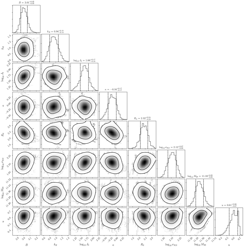
Figure 1: Posterior distributions for the eight model parameters. The black solid curves in the 2D marginalised subspaces enclose $68\%$ and $95\%$ of the total probability. The black vertical dashed lines in the 1D marginalised subspaces are the 16th and 84th percentiles.

4.3 Posterior

We sampled the posterior distribution $P(\boldsymbol{\Xi}|{\bf w})$ of the model parameters via a Markov chain Monte Carlo (MCMC) method. We used a Metropolis-Hastings sampler (Hastings 1970) with a multi-variate proposal distribution. We ran 50 independent chains for 3000 steps, which were found to converge after a short burn-in phase of about $\sim 600$ steps, thus we effectively sampled the posterior distribution with $\sim 120,000$ samples. All the chains turned out to be well mixed and we tuned the parameters of the proposal distribution to have $\sim 40-60\%$ acceptance rate and small auto-correlations (after burn-in).

5 Results

Figure 1 shows the 1D and 2D marginalised posterior distributions of the eight free parameters of our model. All the parameters are relatively well constrained by our analysis, with relative uncertainties limited to $\sim 10\%$. In what follows we always associate error bars with each measurement representing the 16th and 84th percentiles of the marginalised posterior distribution. Figure 1 depicts some non-zero correlations between the parameters which we discuss below.

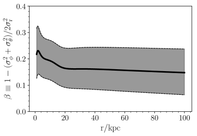
Figure 2: Spherically averaged velocity anisotropy profile of the halo component of the GC system. The black solid line is for our best model and the grey band encompasses the 16th and 84th percentiles of the distribution.

5.1 Distribution function

5.1.1 Halo

The halo DF of the best model has a shallow slope ($B=3.01\pm 0.05$) and a small-scale action ($J_{0}=46^{+22}_{-15}$ kpc km s^-1) and we find these two quantities to be correlated as models with a steeper slope have a larger scale action. This degeneracy is not surprising, and it is inevitable since $J_{0}$ controls the physical scale at which the spatial density profile steepens. Our best model has a very small constant density core, of $\sim 0.1$ kpc, and its density distribution is a power law close to $\rho\propto r^{-3.3}$.

Contrary to previous claims (e.g. BW17, ), we find the halo component not to be significantly rotating ($\kappa=-0.14\pm 0.14$), if not mildly counter-rotating. In fact, in our best model the halo component has a small net retrograde rotation of the order of $V_{\rm rot}\sim-14$ km/s at 20 kpc (roughly consistent with other independent estimates, e.g. Beers et al. 2012; Kafle et al. 2017; Koppelman, Helmi, & Veljanoski 2018), while the disc component is rotating at about $V_{\rm rot}\sim 210$ km/s at the solar radius. This difference compared to previous work is due to the dramatic increase in data quality.

We also constrain relatively well the coefficient $k_{R}$ of the homogeneous function $g({\bf J})$ entering in the halo DF definition, and which controls the velocity anisotropy of the halo component. Our best model with $k_{R}=0.94^{+0.15}_{-0.14}$ has a mildly radially biased velocity distribution, with a rather constant $\beta\equiv 1-(\sigma_{\phi}^{2}+\sigma_{\phi}^{2})/2\sigma_{r}^{2}\simeq 0.15-0.2$, consistent with previous measurements (e.g. Eadie, Springford, & Harris 2017). We show in Figure 2 the spherically averaged anisotropy profile of the halo component.

5.1.2 Disc

The disc DF is consistent with that of the Galactic thick disc fitted by Piffl et al. (2014b): the scale-length of the disc is $R_{\rm d}=2.32^{+0.24}_{-0.23}$ kpc (see Table 1), while the central radial velocity dispersion is $\sigma_{R,0}=132^{+23}_{-22}$ km/s. However, given that we have fixed two of the DF parameters, $R_{\sigma}$ and $h_{\rm d}$, to resemble the thick disc, it comes as no surprise that we find agreement with the estimates by Piffl et al. (2014b). This serves more as a sanity check that the MCMC chains are converging to a physical solution, instead of a proper constraint. The fact that we find the most likely models precisely in the region of the parameter space where the Galactic thick disc is, implies that our analysis is consistent with the possibility that some GCs were born in the thick disc or were associated with its formation (e.g. Zinn 1985).

5.1.3 Spatial and velocity distribution

We now compare the observed and predicted spatial and velocity distributions of the GC system. In Figure 3 we show the heliocentric distance distribution of the full sample of 143 GCs compared to that of our best model. For visualisation purposes, we have cut both distributions at $50$ kpc. The model represents very well the observed distances to the cluster: running a Kolmogorov-Smirnov test on the full sample (143 GCs) we find a $63^{+15}_{-10}\%$ probability that they are drawn from the same distribution. It turns out that most of the numerical noise in this comparison comes from the six clusters found at distances between $50$ and $120$ kpc: if we exclude this large and very poorly sampled volume and we restrict the comparison to the clusters within 50 kpc we find a probability of $93^{+5}_{-4}\%$ that the data and model come from the same underlying distribution. Within 50 kpc, the largest discrepancy is found between 10 and 30 kpc, but it is not significant (see inset in Fig. 3).

For the first time we have a sufficiently large dataset of accurate proper motions of 91 GCs, and we can also make a meaningful comparison with the velocity distribution predicted by the model. We show in Figure 4 the cumulative distributions of three cartesian heliocentric velocities $(V_{x},V_{y},V_{z})$, where $V_{x}$ points towards the Galactic centre and $V_{Y}$ is parallel to the Galactic disc’s rotation. Figure 5 also shows the 2D projections of the clusters velocity distribution compared to the models.

The agreement between data and model is generally very good; however, it should be noted that the model appears somewhat more symmetric with respect to the observed velocity distribution of GCs. On the one hand, it should be kept in mind that our equilibrium models will always produce symmetric distributions in $V_{x}$ and $V_{z}$; on the other hand, observed deviations from symmetry may be due to the presence of substructures or may simply be stochastic, due to the small number of tracers (91).

5.1.4 Metallicity distribution

For each model we can use Eq. (12) to compute the probability that a cluster belongs to the disc component rather than to the halo by substituting $f$ with $f_{\rm disc}$ or $f_{\rm halo}$, respectively. The ratio of these two probabilities, which we call $P_{\rm disc}$ and $P_{\rm halo}$, can be used to estimate the membership of each GC to these components. We now compare these membership probabilities with the metallicity [Fe/H] of each cluster, whose distribution is bimodal with a minimum at [Fe/H]$\simeq-0.8$ that has been classically used to distinguish metal-poor halo clusters from metal-rich disc ones (e.g. Zinn 1985).

Figure 6 shows the metallicity of the 143 GCs as a function of the logarithm of the ratio $P_{\rm disc}/P_{\rm halo}$ in our best model. Similarly to BW17, we find that metal-rich clusters are typically much more likely to belong to the disc component rather than the halo, with only a couple of exceptions. In particular, all but two clusters with [Fe/H]$>-0.8$ have $\log_{10}(P_{\rm disc}/P_{\rm halo})>-2$, making it very unlikely that they are a part of the halo component (see histogram in the bottom panel of Fig. 6). At lower metallicities, instead, there are many more clusters with $\log_{10}(P_{\rm disc}/P_{\rm halo})<-2$ ($67\%$ below [Fe/H]$\leq-0.8$), making them very likely halo clusters. These are typically objects that are either found at very large distances, that are counter-rotating, or that have negligible angular momentum. Figure 6 shows that only a few clusters with heliocentric distances larger than 20 kpc have a higher probability of being part of the disc component.

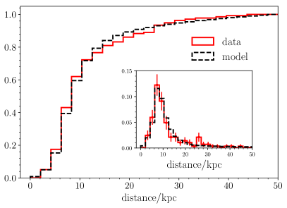
Figure 3: Cumulative distribution of heliocentric distances of the 143 GCs (red solid) compared to that of the best model (black dashed). We cut these at $50$ kpc for illustration purposes. The Kolmogorov-Smirnov test returns a $63\%$ probability that the two samples are drawn from the same distribution. The inset shows the normalised distribution of distances within $30$ kpc with Poissonian error bars.

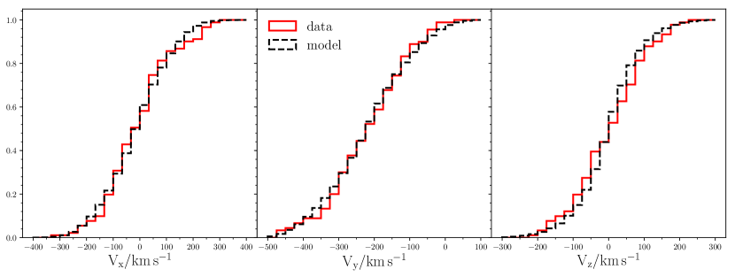
Figure 4: Cumulative distribution of heliocentric cartesian velocities of the GCs (red solid) compared to that of the best model (black dashed). The Kolmogorov-Smirnov test returns a $88\%$, $83\%$, and $42\%$ probability that the two samples in $V_{x}$, $V_{y}$, and $V_{z}$, respectively, are drawn from the same distributions.

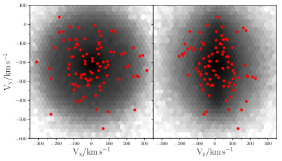
Figure 5: Velocity distribution in the $V_{x}-V_{y}$ and $V_{z}-V_{y}$ planes of the model (black) compared to that of the data (red circles).

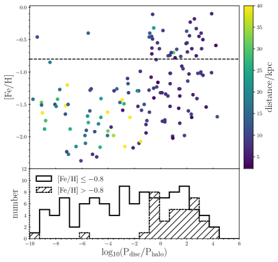
Figure 6: Upper panel: Metallicity of the GCs as a function of the ratio of the probability of belonging to the disc or the halo component of the DF. The points are colour-coded according to the heliocentric distance of the cluster. The horizontal dashed line marks [Fe/H]=-0.8, the classical distinction between metal-poor and metal-rich clusters. Lower panel: Histogram of the ratio of probabilities in two bins of metal-rich ([Fe/H]$>$-0.8) and metal-poor ([Fe/H]$\leq$-0.8) clusters.

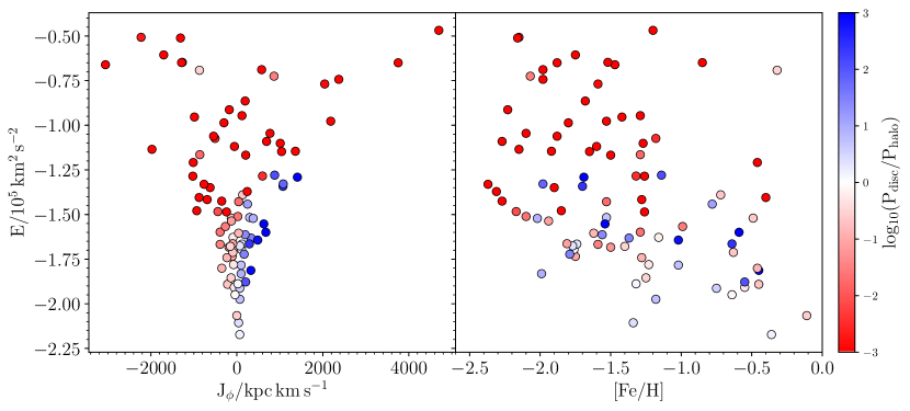
Figure 7: Left panel: Distribution of the 91 GCs with accurate proper motions in the angular momentum-energy plane, colour-coded by the ratio of probability of belonging to the disc or to the halo. Right panel: Same as the left panel, but in the metallicity-energy plane.

In the left-hand panel of Figure 7 we show the distribution of the 91 clusters with accurate proper motions in the plane of integrals of motion angular momentum-energy, colour-coded by $\log_{10}(P_{\rm disc}/P_{\rm halo})$. Here we see that all clusters less bound than $E\gtrsim-1.25\times 10^{5}\,\rm km\,s^{-1}$ belong to the halo component. At lower (more negative) energies, halo clusters clearly prefer retrograde ($J_{\phi}<0$) or non-rotating ($J_{\phi}\sim 0$) orbits, while the probability of belonging to the disc component is maximal for prograde angular momenta. For the likely disc clusters ($\log_{10}P_{\rm disc}/P_{\rm halo}>0$) we find an average angular momentum of $\overline{J}_{\phi}=364\pm 71\,\rm kpc\,km\,s^{-1}$, while for the very likely halo clusters ($\log_{10}P_{\rm disc}/P_{\rm halo}<0$) we find $\overline{J}_{\phi}=-164\pm 112\,\rm kpc\,km\,s^{-1}$, from which we conclude that the halo clusters exhibit a hint of retrograde rotation. If we divide the sample of 91 GCs according to the traditional separation into metal-rich [Fe/H]$>-0.8$ (18 clusters) and metal-poor [Fe/H]$\leq-0.8$ (73 clusters), we find a mean $z$-angular momentum of respectively $\overline{J}_{\phi}=-70\pm 120\,\rm kpc\,km\,s^{-1}$ and $\overline{J}_{\phi}=17\pm 100\,\rm kpc\,km\,s^{-1}$ for the two populations. This is because some metal-rich clusters are on low-energy, sometimes even retrograde orbits, while a few clusters on disc-like orbits happen to have low metallicity.

The right-hand panel of Figure 7 shows energy as a function of metallicity, with the points being again colour-coded by their membership probability. It can be seen that the metal-poor halo clusters are mostly confined to less bound orbits, while disc clusters with high angular momentum span a wide range of metallicities.

5.2 Gravitational potential

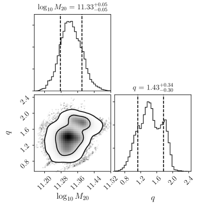
Figure 8: Posterior distributions of the two parameters describing the Galaxy’s dark halo: the total mass of the Galaxy within 20 kpc, $M_{20}$, and the axis ratio of the dark halo, $q$. The number of bins is increased with respect to Fig. 1. Black solid curves and vertical dashed lines are as in Fig. 1.

With our modelling technique we are able to constrain the characteristic parameters of the Galaxy’s inner dark matter halo that fit the observed dynamics of GCs. The main novelty of our work is the fact that the new dataset released by the Gaia Collaboration et al. (2018b) gives us strong inference on both the total mass and shape of the dark matter halo. In particular, in Figure 8 we show the posterior distribution of the Galaxy’s mass within 20 kpc and the halo’s axis ratio $q$ as sampled by our MCMC analysis. We find that $\log_{10}M_{20}/M_{\odot}=11.33\pm 0.05$ and $q=1.43^{+0.34}_{-0.30}$ and that they are strongly correlated with more massive halos being more prolate. While such a degeneracy is expected (e.g. Bowden, Evans, & Williams 2016), here we nonetheless find that spherical and light halos are disfavoured by our analysis, while halos more oblate than $q\leq 0.8$ are ruled out with $99\%$ probability by our experiment, as are strongly prolate halos with $q\geq 1.9$.

The posterior distribution that we sample is not unimodal, but it has two distinct peaks; the most likely is at $\log_{10}M_{20}\simeq 11.33$, $q\simeq 1.37$ and the other at $\log_{10}M_{20}\simeq 11.38$, $q\simeq 1.75$. Although it is located in a region where the likelihood is considerably lower, the second peak cannot be neglected and deserves further investigation.

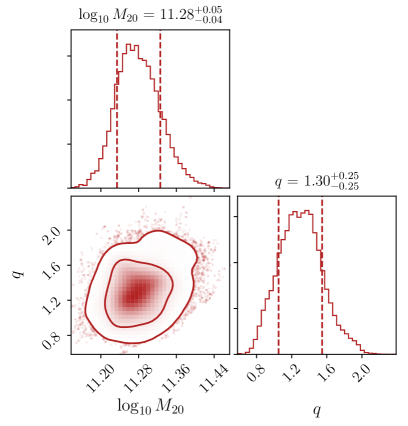
Figure 9: Same as Fig. 8, but obtained excluding the GCs associated with the Sagittarius dwarf galaxy.

As discussed in the introduction, an important number of GCs in our sample are likely associated with the Sagittarius dwarf galaxy and have thus been accreted on similar orbits. In this case, our assumption that all the GCs are a random sample of our DF breaks down, and this could lead to biases in the results of the modelling. We therefore remove the clusters mentioned in Sec. 2.2, and repeat the analysis outlined in Sect. 4. As a result we obtain the posterior distribution for the halo parameters shown in Figure 9. Now the second lower peak has completely disappeared and the distribution has a well-constrained peak at $\log_{10}M_{20}/M_{\odot}=11.28\pm 0.04$ and $q=1.22\pm 0.23$. From this we conclude that the second peak was most probably driven by the few clusters on very polar orbits dynamically associated with the Sagittarius dwarf galaxy.

Within 20 kpc, we find the total mass of the Galaxy to be $1.91^{+0.18}_{-0.17}\times 10^{11}M_{\odot}$, which implies a dark matter mass of $1.37^{+0.18}_{-0.17}\times 10^{11}M_{\odot}$. If we extrapolate this to the virial radius, assuming a concentration-mass relation as calibrated from numerical simulations (Dutton & Macciò 2014), we obtain the following final estimate of the Galaxy’s dark matter halo mass,

$$M_{\rm vir}=1.3\pm 0.3\times 10^{12}M_{\odot}$$ (14)

and thus a virial radius of $r_{\rm vir}=287^{+22}_{-25}$ kpc.

Many different studies have already estimated the mass of the dark matter halo of the Milky Way using very different techniques and tracers, which typically are sensitive to very different physical scales. Thus, a proper comparison taking into account all the possible biases given by the different assumptions or data used is needed, but it goes beyond the scope of the present study. By naively comparing our results with the numerical estimates compiled by Bland-Hawthorn & Gerhard (2016, and references therein) and Eadie & Harris (2016, and references therein) we conclude that our estimate of $M_{20}$ and of the extrapolated $M_{\rm vir}$ lies somewhere between the very light ($M_{\rm vir}<10^{12}M_{\odot}$, e.g. Battaglia et al. 2005; Gibbons, Belokurov, & Evans 2014) and of the very heavy values ($M_{\rm vir}>2\times 10^{12}M_{\odot}$ Li & White 2008; Watkins, Evans, & An 2010). In general, we find good agreement with other works that use satellite kinematics (provided that distant enough tracers are included, e.g. Boylan-Kolchin et al. 2013; Gonzalez et al. 2013; Eadie & Harris 2016; Patel et al. 2018; Sohn et al. 2018), estimates of the escape velocity (e.g. Smith et al. 2007; Piffl et al. 2014a), the velocity distribution of either fast moving stars (e.g. Gnedin et al. 2010), or the dynamics of nearby stars (e.g. McMillan 2011; Piffl et al. 2014b).

Similarly, there has also been some work on the shape of the total gravitational potential. While a proper comparison taking into account the systematics induced by tracers and methods is not straightforward, here we note that our estimate roughly agrees with other studies of the Sagittarius stream (Helmi 2004), the flaring of the HI disc (Banerjee & Jog 2011), or the kinematics of halo stars (Bowden, Evans, & Williams 2016), while being apparently inconsistent with studies modelling the GD-1 stream (Koposov, Rix, & Hogg 2010; Bowden, Belokurov, & Evans 2015, which, however, probes a region much closer to the Galactic centre) and studies of the tilt of the local velocity ellipsoid (Smith, Wyn Evans, & An 2009; Posti et al. 2018).

It may well be the case that the shape of the halo of our Galaxy is considerably more complicated than we have assumed here; for instance, i) it can be axisymmetric, but with a variable flattening as a function of radius (e.g. Vera-Ciro & Helmi 2013), being oblate close to the disc and more spherical/prolate at greater distances (e.g. as probed by the HI disc flare, Banerjee & Jog 2011); ii) it can be triaxial (e.g. as probed by the modelling of the Sagittarius stream Law & Majewski 2010); or iii) it can be triaxial, but with variable axis ratios/orientations as a function of radius (e.g. as expected from numerical simulations, Bailin & Steinmetz 2005; Vera-Ciro et al. 2011, and as probed by the Sagittarius stream, Vera-Ciro & Helmi 2013). Different results are thus found both because of different model assumptions and because of the various observables used: since different tracers are probably sensitive to distinct portions of the halo, the methodologies used to infer the halo shape may be subject to different kinds of limitations. This implies that to make further progress in our understanding of the shape of the dark halo of the Milky Way it is imperative to combine the signal coming from tracers of different nature.

6 Conclusions

We have used the kinematics of Milky Way GCs to simultaneously constrain the phase-space distribution of the GC system, the mass of the inner Galaxy, and the shape of its inner dark matter halo. This was possible thanks to the novel measurements by Gaia and HST of the proper motions of 91 GCs with unprecedented accuracy.

Our method is based on the assumption that the GC system can be described by axisymmetric equilibrium models with two distribution functions, which are analytic functions of the action integrals, representing the phase-space distribution of disc and halo clusters. Our models include an axisymmetric NFW dark matter halo, whose mass and density axis ratio, have been determined by fitting the kinematics of 143 GCs (91 with accurate 6D data and 52 with only radial velocities), using a Bayesian approach, imposing uninformative priors on the eight model characteristic parameters.

We summarise here our main results:

• we find all the parameters of the halo component to be well constrained. The density distribution is well described by a single power law $\rho\propto r^{-3.3}$; the velocity distribution is mildly radially biased, with a rather constant anisotropy $\beta\simeq 0.2\pm 0.07$, and consistent with either a small counter-rotation ($V_{\rm rot}\simeq-15\,\rm km\,s^{-1}$ at 20 kpc) or no net rotation;

• we find all the parameters of the disc component to be well constrained. Their phase-space distribution closely resembles that of the thick disc of the Galaxy (Piffl et al. 2014b);

• metal-rich clusters ([Fe/H]$>-0.8$) very likely belong to the disc component, while roughly $67\%$ of the metal-poor clusters ([Fe/H]$\lesssim-0.8$) are more likely part of the halo component. All clusters with low binding energies belong to the halo component and have both prograde and retrograde orbits. The more bound halo clusters are typically found on counter-rotating or non-rotating orbits. Most metal-rich clusters ([Fe/H]$\gtrsim-0.8$) have high a probability of being associated with the disc component. Our findings are broadly consistent with the picture proposed by Zinn (1985);

• we measure the mass of the dark matter halo of the Galaxy within 20 kpc to be $\log_{10}M_{20,\rm DM}/M_{\odot}=11.14\pm 0.05$. This very accurate measurement implies a total virial mass for the Milky Way of $M_{\rm vir}=1.3\pm 0.3\times 10^{12}M_{\odot}$ after assuming a concentration-virial mass relation;

• we measure a flattening $q=1.22\pm 0.23$, and find oblate halos with $q<0.7$ to be ruled out by our analysis (with $99\%$ probability) and spherical models to be disfavoured in comparison to prolate halos.

During the completion of this work, Watkins et al. (2018) presented an estimate of the Milky Way’s dark halo mass by applying a simple ‘tracer mass estimator’ on a similar dataset. Their values for the mass within 21.1 kpc (and within the virial radius) are closely compatible with ours, as is their measurement of the anisotropy (although they favour a slightly more radially biased ellipsoid).

Our work demonstrates that with a giant leap in data quality such as that provided by the Gaia DR2, constraints on fundamental physical quantities become significantly more precise, and several of these parameters can be determined at once if models with enough sophistication are employed. Of course, with this work we have simply touched the tip of the iceberg of the signal present in the Gaia data regarding the mass and shape of the Galactic potential. The next challenge will be to simultaneously fit the dynamics of different mass tracers such as satellites, streams, field stars in the halo, and hypervelocity stars. This work may be seen as a necessary first step in this direction, and merely confirms that we may have just entered the era of ‘Precision Galactic Astronomy’.