Scrambled Linear Pseudorandom Number Generators

Abstract.

$\mathbf{F}_{2}$-linear pseudorandom number generators are very popular due to their high speed, to the ease with which generators with a sizable state space can be created, and to their provable theoretical properties. However, they suffer from linear artifacts that show as failures in linearity-related statistical tests such as the binary-rank and the linear-complexity test. In this paper, we give two new contributions. First, we introduce two new $\mathbf{F}_{2}$-linear transformations that have been handcrafted to have good statistical properties and at the same time to be programmable very efficiently on superscalar processors, or even directly in hardware. Then, we describe some scramblers, that is, nonlinear functions applied to the state array that reduce or delete the linear artifacts, and propose combinations of linear transformations and scramblers that give extremely fast pseudorandom number generators of high quality. A novelty in our approach is that we use ideas from the theory of filtered linear-feedback shift registers to prove some properties of our scramblers, rather than relying purely on heuristics. In the end, we provide simple, extremely fast generators that use a few hundred bits of memory, have provable properties, and pass strong statistical tests.

1. Introduction

In the last twenty years, in particular since the introduction of the Mersenne Twister (Matsumoto and Nishimura, 1998), $\mathbf{F}_{2}$-linear pseudorandom number generators have been very popular: indeed, they are often the stock generator provided by several programming languages. Linear generators have several advantages: they are fast, it is easy to create full-period generators with large state spaces, and thanks to their connection with linear-feedback shift registers (LFSRs) (Klein, 2013) many of their properties, such as full period, are mathematically provable. Moreover, if suitably designed, they are rather easy to implement using simple xor and shift operations.

The linear structure of such generators, however, is detectable by some statistical tests for randomness: in particular, the binary-rank test (Marsaglia and Tsay, 1985) and the linear-complexity test (Carter, 1989; Erdmann, 1992) are failed by all linear generators. Such tests are implemented, for example, by the testing framework TestU01 (L’Ecuyer and Simard, 2007) under the name “MatrixRank" and “LinearComp”, respectively. These tests were indeed devised to “catch” linear generators, and they are not considered problematic by the community working on such generators, as the advantage of being able to prove precise mathematical properties is perceived as outweighing the failure of such tests (see (Vigna, 2019) for a more detailed discussion).

Nonetheless, one might find it desirable to mitigate or eliminate such linear artifacts by scrambling a linear generator, that is, applying a nonlinear function to its state array to produce the actual output. In this direction, two simple approaches are multiplication by a constant or adding two components of the state array. However, while empirical tests usually do not show linear artifacts anymore, the lower bits are unchanged or just slightly modified by such operations. Thus, those bits in isolation (or combined with a sufficiently small number of good bits) will fail linearity tests.

In this paper, we try to find a middle ground by proposing very fast scrambled generators with provable properties. By combining in different ways an underlying linear engine and a scrambler we can provide different tradeoffs in terms of speed, space usage, and statistical quality.

For example, xoshiro256++ is a $64$-bit generator with 256 bits of state that emits a value in $0.86$ ns on an Intel® Core™ i7-8700B CPU @$3.20$ GHz (see Table 1 for details); it passes all statistical tests we are aware of, and it is $3$-dimensionally equidistributed. Multiple instances can be easily parallelized using Intel’s extended AVX2 instruction set, reducing the time to $0.30$ ns (for eight instances). Similarly, xoshiro256** is $4$-dimensionally equidistributed, but it has a lower linear complexity.

However, if the user is interested in the generation of floating-point numbers only, we provide a xoshiro256+ generator that generates a value in $0.78$ ns (the value must then be converted to float); it is just $3$-dimensionally equidistributed, and its lowest bits have low linear complexity, but since one needs just the upper $53$ bits, the resulting floating-point values have no linear bias. As in the previous case, instances can be parallelized, bringing down the time to $0.22$ ns.

If space is an issue, a xoroshiro128++, xoroshiro128**, or xoroshiro128+ generator provides similar timings and properties in less space. We also describe higher-dimensional generators, albeit mainly for theoretical reasons, and $32$-bit generators with similar properties that are useful for embedded devices and GPUs. Our approach can even provide fast, reasonable $16$-bit generators.

Finally, we develop some theory related to our linear engines and scramblers using results from the theory of noncommutative determinants and from the theory of filtered LFSRs.

The C code for the generators described in this paper is available from the authors and it is public domain. The test code is distributed under the GNU General Public License version 3 or later.

2. Organization of the paper

In this paper, we consider words of size $w$, $w$-bit operations, and generators with $kw$ bits of state, $k\geq 2$. We aim mainly at $64$-bit generators (i.e., $w=64$), but we also provide $32$-bit combinations.

The paper is organized in such a way to make immediately available code and basic information for our new generators as quickly as possible: all theoretical considerations and analyses are postponed to the second part of the paper, albeit sometimes this approach forces us to point at subsequent material.

Our generators consist of a linear engine and a scrambler. The linear engine is a linear transformation on $\mathbf{Z}/2\mathbf{Z}$, representable by a matrix, and it is used to advance the internal state of the generator. The scrambler is an arbitrary function on the internal state which computes the actual output of the generator. We will usually apply the scrambler to the current state, to make it easy for the CPU to parallelize internally the operations of the linear engine and of the scrambler. Such a combination is quite natural: for example, it was advocated by Marsaglia for xorshift generators (Marsaglia, 2003), by Panneton and L’Ecuyer in their survey (L’Ecuyer and Panneton, 2009), and it has been used in the design of XSAdd (Saito and Matsumoto, 2014) and of the Tiny Mersenne Twister (Saito and Matsumoto, 2015). An alternative approach is that of combining an $\mathbf{F}_{2}$-linear generator with a linear congruential generator with large prime modulus (L’Ecuyer and Granger-Piché, 2003).

In Section 3 we introduce our linear engines. In Section 4 we describe the scramblers we will be using and their elementary properties. Finally, in Section 5 we describe generators given by several combinations between scramblers and linear engines, their speed and their results in statistical tests. Section 5.3 contains a guide to the choice of an appropriate generator.

In Section 6 and 7 we discuss the mathematical properties of our linear engines: in particular, we introduce the idea of word polynomials, polynomials on $w\times w$ matrices associated with a linear engine. The word polynomial makes it easy to compute the characteristic polynomial, which is the basic tool to establish full period. We then provide equidistribution results.

In the last part of the paper, starting with Section 9, we apply ideas and techniques from the theory of filtered LFSRs to the problem of analyzing the behavior of our scramblers. We provide some exact results and discuss a few heuristics based on extensive symbolic computation. Our discussion gives a somewhat more rigorous foundation to the choices made in Section 5, and opens several interesting problems.

3. Linear engines

In this section we introduce our two linear engines xoroshiro (xor/rotate/shift/rotate) and xoshiro (xor/shift/rotate). All modern C/C++ compilers can compile a simulated rotation into a single CPU instruction, and Java provides intrinsified rotation static methods to the same purpose. As a result, rotations are no more expensive than a shift, and they provide better state diffusion, as no bit of the operand is discarded.

We denote with $S$ the $w\times w$ matrix on $\mathbf{Z}/2\mathbf{Z}$ that effects a left shift of one position on a binary row vector (i.e., $S$ is all zeroes except for ones on the principal subdiagonal) and with $R$ the $w\times w$ matrix on $\mathbf{Z}/2\mathbf{Z}$ that effects a left rotation of one position (i.e., $R$ is all zeroes except for ones on the principal subdiagonal and a one in the upper right corner). We will use $\rho_{r}(-)$ to denote left rotation by $r$ of a $w$-bit vector in formulae; in code, we will write rotl(-,r).

3.1. xoroshiro

The xoroshiro linear transformation updates cyclically two words of a larger state array. The update rule is designed so that data flows through two computation paths of length two with a single common dependency halfway, leading to good parallelizability inside superscalar CPUs.

The base xoroshiro linear transformation is obtained combining a rotation, a shift, and again a rotation (hence the name), and it is defined by the following $2w\times 2w$ matrix:

$$\mathscr{X}_{2w}=\left(\begin{matrix}R^{a}+S^{b}+I&R^{c}\\ S^{b}+I&R^{c}\\ \end{matrix}\right).$$

The general $kw\times kw$ form is given instead by

(1) $$\mathscr{X}_{kw}=\left(\begin{matrix}0&0&\cdots&0&R^{a}+S^{b}+I&R^{c}\\ I&0&\cdots&0&0&0\\ 0&I&\cdots&0&0&0\\ \cdots&\cdots&\cdots&\cdots&\cdots&\cdots\\ 0&0&\cdots&I&0&0\\ 0&0&\cdots&0&S^{b}+I&R^{c}\end{matrix}\right)$$

Note that the general form applies the basic form to the first and last words of state, and uses the result to replace the last and next-to-last words. The remaining words are shifted by one position.

The structure of the transformation may appear repetitive, but it has been so designed because this implies a very simple and efficient computation path. Indeed, in Figure 1 we show the C code implementing the xoroshiro transformation for $w=64$ with $128$ bits of state. The constants prefixed with “result” are outputs computed using different scramblers, which will be discussed in Section 4. The general case is better implemented using a form of cyclic update, as shown in Figure 2.

The reader should note that after the first xor, which represents the only data dependency between the two words of the state array, the computation of the two new words can continue in parallel, as depicted graphically in Figure 3.

    const uint64_t s0 = s[0];
    uint64_t s1 = s[1];

    const uint64_t result_plus = s0 + s1;
    const uint64_t result_plusplus = rotl(s0 + s1, R) + s0;
    const uint64_t result_star = s0 * S;
    const uint64_t result_starstar = rotl(s0 * S, R) * T;

    s1 ^= s0;
    s[0] = rotl(s0, A) ^ s1 ^ (s1 << B);
    s[1] = rotl(s1, C);

Figure 1. The C code for a xoroshiro128+/xoroshiro128++/xoroshiro128*/xoroshiro128** generator. The array s contains two $64$-bit unsigned integers, not all zeros.

    const int q = p;
    const uint64_t s0 = s[p = (p + 1) & 15];
    uint64_t s15 = s[q];

    const uint64_t result_plus = s0 + s15;
    const uint64_t result_plusplus = rotl(s0 + s15, R) + s15;
    const uint64_t result_star = s0 * S;
    const uint64_t result_starstar = rotl(s0 * S, R) * T;

    s15 ^= s0;
    s[q] = rotl(s0, A) ^ s15 ^ (s15 << B);
    s[p] = rotl(s15, C);

Figure 2. The C code for a xoroshiro1024+/xoroshiro1024++/xoroshiro1024*/xoroshiro1024** generator. The state array s contains sixteen $64$-bit unsigned integers, not all zeros, and the integer variable $p$ holds a number in the interval $[0\,\mathpunct{\ldotp\ldotp}16)$.

Figure 3. The dependency paths of the xoroshiro128 linear engine. Data flows from top to bottom: lines converging to a box are xor’d together, and labels represent $w\times w$ linear transformations applied to the data flowing through the line. Note that the linear transformation $S^{b}+I$ is a xorshift.

3.2. xoshiro

The xoshiro linear transformation uses only a shift and a rotation. Since it updates all of the state at each iteration, it is sensible only for moderate state sizes. We will discuss the $4w\times 4w$ and $8w\times 8w$ transformations

$$\mathscr{S}_{4w}=\left(\begin{matrix}I&I&I&0\\ I&I&S^{a}&R^{b}\\ 0&I&I&0\\ I&0&0&R^{b}\\ \end{matrix}\right)\qquad\qquad\mathscr{S}_{8w}=\left(\begin{matrix}I&I&I&0&0&0&0&0\\ 0&I&0&0&I&I&S^{a}&0\\ 0&I&I&0&0&0&0&0\\ 0&0&0&I&0&0&I&R^{b}\\ 0&0&0&I&I&0&0&0\\ 0&0&0&0&I&I&0&0\\ I&0&0&0&0&0&I&0\\ 0&0&0&0&0&0&I&R^{b}\\ \end{matrix}\right).$$

The layout of the matrices above might seem arbitrary, but it is just derived from the implementation. In Figure 4 and 5 is it easy to see the algorithmic structure of a xoshiro transformation: the second word of the state array is shifted and stored; then, in order all words of the state array are xor’d with a different word; finally, the shifted part is xor’d into the next-to-last word of the state array, and the last word is rotated. The shape of the matrix depends on the order chosen for the all-words xor sequence. Figure 6 shows that also for xoshiro256 dependency paths are very short, and similarly happens for xoshiro512.

Note that xoshiro is not definable for a state of $2w$ bits, and it is too slow for a state of $16w$ bits, because of the large number of write operations required at each iteration.

    const uint64_t result_plus = s[0] + s[3];
    const uint64_t result_plusplus = rotl(s[0] + s[3], R) + s[0];
    const uint64_t result_starstar = rotl(s[1] * S, R) * T;

    const uint64_t t = s[1] << A;
    s[2] ^= s[0];
    s[3] ^= s[1];
    s[1] ^= s[2];
    s[0] ^= s[3];
    s[2] ^= t;
    s[3] = rotl(s[3], B);

Figure 4. The C code for a xoshiro256+/xoshiro256++/xoshiro256** generator. The state array s contains four $64$-bit unsigned integers, not all zeros.

    const uint64_t result_plus = s[0] + s[2];
    const uint64_t result_plusplus = rotl(s[0] + s[2], R) + s[2];
    const uint64_t result_starstar = rotl(s[1] * S, R) * T;

    const uint64_t t = s[1] << A;
    s[2] ^= s[0];
    s[5] ^= s[1];
    s[1] ^= s[2];
    s[7] ^= s[3];
    s[3] ^= s[4];
    s[4] ^= s[5];
    s[0] ^= s[6];
    s[6] ^= s[7];
    s[6] ^= t;
    s[7] = rotl(s[7], B);

Figure 5. The C code for a xoshiro512+/xoshiro512++/xoshiro512** generator. The state array s contains eight $64$bit unsigned integers, not all zeros.

Figure 6. The data dependencies of the xoshiro256 linear engine.

4. Scramblers

Scramblers are nonlinear mappings from the state of the linear engine to a $w$-bit value, which will be the output of the generator. The purpose of a scrambler is to improve the quality of the raw output of the linear engine: since in general linear transformations have several useful provable properties, this is a practical approach to obtain a fast, high-quality generator.

4.1. Sum

The + scrambler simply adds two words of the state array in $\mathbf{Z}/2^{w}\mathbf{Z}$. The choice of words is relevant to the quality of the resulting generator, and we performed several statistical tests to choose the best pair depending on the underlying engine. The idea appeared in Saito and Matsumoto’s XSadd generator (Saito and Matsumoto, 2014), and was subsequently used by the xorshift+ family (Vigna, 2016b).

Note that the lowest bit output by the + scrambler is just a xor of bits following the same linear recurrence, and thus follows, in turn, the same linear recurrence. For this reason, we consider + a weak scrambler. As we consider higher bits, there is still a linear recurrence describing their behavior, but it becomes quickly of such a high linear complexity to become undetectable. We will discuss in more detail this issue in Section 9. In the sample code, the result_plus output is computed using the + scrambler.

4.2. Multiplication

The * scrambler multiplies by a constant a chosen word of the state array, and since we are updating more than a word at a time, the choice of the word is again relevant. Its only parameter is the multiplier. The multiplier must be odd, so that the scrambling is a bijection; moreover, if the second-lowest bit set is in position $b$, the lowest $b$ bits of the output are unmodified, and the following bit is a xor of bit $0$ and bit $b$, so it follows the same linear recurrence as the lower bits, as it happens for the lowest bit of the + scrambler. For this reason, we consider also * a weak scrambler.

We will use multipliers close to $\varphi 2^{w}$, where $\varphi$ is the golden ratio, as $\varphi$ is an excellent multiplier for multiplicative hashing (Knuth, 1997). To minimize the number of unmodified bits, however, we will adjust the lower bits in such a way that bit 1 is set. In the sample code, the result_star output is computed using the * scrambler.

4.3. Sum, rotation, and again sum

The ++ scrambler uses two words of the state array: the two words are summed in $\mathbf{Z}/2^{w}\mathbf{Z}$, the sum is rotated to the left by $r$ positions, and finally we add in $\mathbf{Z}/2^{w}\mathbf{Z}$ the first word to the rotated sum. Note that the choice and the order are relevant—the ++ scrambler on the first and last word of state is different from the ++ scrambler on the last and first word of state. Besides the choice of words, we have to specify the amount $r$ of left rotation. Since the rotation moves the highest bits obtained after the first sum to lower bits, it is easy to set up the parameters so that there are no bits of low linear complexity in the output. For this reason, we consider ++ a strong scrambler. In the sample code, the result_plusplus output is computed using the ++ scrambler.

4.4. Multiplication, rotation, and again multiplication

The ** scrambler is given by a multiply-rotate-multiply sequence applied to a chosen word of the state array (again, since we are updating more than a word at a time, the choice of the word is relevant). It thus requires three parameters: the first multiplier, the amount of left rotation, and the second multiplier; both multipliers should be odd, so that the scrambling is a bijection. As in the case of the ++ scrambler, it is easy to choose $r$ so that there are no bits of low linear complexity in the output, so ** is a strong scrambler.

We will mostly use multipliers of the form $2^{s}+1$, which are usually computed very quickly, and which have the advantage of being alternatively implementable with a left shift by $s$ and a sum (the compiler should make the right choice, but one can also benchmark both implementations). In the sample code, the result_starstar output is computed using the ** scrambler.

5. Combining linear engines and scramblers

In this section we discuss several interesting combinations of linear engines and scramblers, both for the $64$-bit and the $32$-bit case, and report results of empirical tests. We remark that all our generators, being based on linear engines, have jump functions that make it possible to move ahead quickly by any number of next-state steps. Please refer to (Haramoto et al., 2008; Vigna, 2016b) for a simple explanation.

Part of our experiments use the BigCrush test suite from the well-known framework TestU01 (L’Ecuyer and Simard, 2007). We follow the protocol described in (Vigna, 2016a), which we briefly recall. We sample generators by executing BigCrush starting from several different seeds, using the same setup of (Vigna, 2016a) (in particular, for $64$-bit generators we generate uniform $32$-bit values by returning first the lower and then the upper $32$ bits of each output). We consider a test failed if its $p$-value is outside of the interval $[0.001\,\mathpunct{\ldotp\ldotp}0.999]$. We call systematic a failure that happens for all seeds, and report systematic failures (a more detailed discussion of this choice can be found in (Vigna, 2016a)). Note that we run our tests both on a generator and on the generator obtained by reversing the order of the 64 bits returned.

Moreover, we ran a new test we designed, aimed at detecting Hamming-weight dependencies (Blackman and Vigna, 2020), that is, dependencies in the number of zeros and ones in each output word, which are typical of linear generators with sparse transition matrices. We ran the test until we examined a petabyte ($10^{15}$ bytes) of data, or if we obtained a $p$-value smaller than $10^{-20}$, in which case we reported the amount of data at which we stop. The test is failed by several generators for which the Hamming-weight tests in TestU01 are unable to find any bias (Blackman and Vigna, 2020), even using several times more data than for the BigCrush suite.

Not all the generators we discuss are useful from a practical viewpoint, but discussing several combinations and their test failures brings to light the limitation of each component in a clearer way. If the main interest is a practical choice, we suggest to skip to Section 5.3.

5.1. The $64$-bit case

We consider engines xoroshiro128, xoshiro256, xoshiro512 and xoroshiro1024; parameters are provided in Table 2. However, xoshiro yields generators that have better behavior with respect to the tests reported in the first eight lines of Table 1. All linear engines have obvious linear artifacts, but the xoroshiro engines require an order of magnitude less data to fail our Hamming-weight dependency test. Note that this is not only a matter of size, but also of structure: compare xoshiro512 and xoroshiro1024. Analogously, the + scrambler deletes all bias detectable with our test from the xoshiro generators, but it just improves the resilience of xoroshiro+ by almost three orders of magnitudes.

We then present data on the xoroshiro generators combined with the * scrambler: as the reader can notice, the * scrambler does a much better job at deleting Hamming-weight dependencies, but a worse job at deleting linear dependencies, as xoroshiro128* still fails MatrixRank when reversed. In Section 9 we will present some theory explaining in detail why this happens. Once we switch to the ++ and ** strong scramblers, we are not able to detect any bias.

The parameters for all scramblers are provided in Table 3. The actual state words used by the scramblers are described in the code in Figure 1, 2, 4 and 5. Note that the choice of word for the $64$-bit engine xoroshiro128 applies also to the analogous $32$-bit engine xoroshiro64, and that the choice for xoshiro256 applies also to xoshiro128.

Our speed tests have been performed on an Intel® Core™ i7-8700B CPU @$3.20$ GHz using gcc 8.3.0. We used suitable options to keep the compiler from unrolling loops, or extracting loop invariants, or vectorizing the computation under the hood.

5.2. The $32$-bit case

We consider engines xoroshiro64 and xoshiro128. Most of the considerations of the previous section are valid, but in this case for xoroshiro we suggest * as a weak scrambler: the + scrambler, albeit faster, in this case is too weak. As in the previous case, the lowest bits of the generators using a weak scrambler are linear: however, since the output is just $32$ bits, BigCrush detects this linearity (see failures in the reverse test).

Again, once we switch to the ** and ++ scrambler, we are not able to detect any bias (as for the + scrambler, we do not suggest to use the ++ scrambler with xoroshiro64). The parameters for all scramblers are provided in Table 6.

Table 1. Results of tests for $64$-bit generators and three additional popular generators. The columns “S” and “R” report systematic failures in BigCrush (MR=MatrixRank, i.e., binary rank; LC=LinearComp, i.e., linear complexity). The column “HWD” reports the number of bytes generating a $p$-value smaller than $10^{-20}$ in the test described in (Blackman and Vigna, 2020); no value means that the test was passed after $10^{15}$ bytes. The time to emit a 64-bit integer and the number of clock cycles per byte (reported by PAPI (Terpstra et al., 2010)) were computed on an Intel® Core™ i7-8700B CPU @$3.20$ GHz.

Generator	Failures			ns/64 b	cycles/B
	S	R	HWD
xoroshiro128	MR, LC	MR, LC	$1\times 10^{10}$	$0.81$	$0.32$
xoshiro256	MR, LC	MR, LC	$6\times 10^{13}$	$0.72$	$0.29$
xoshiro512	MR, LC	MR, LC	—	$0.83$	$0.39$
xoroshiro1024	MR, LC	MR, LC	$5\times 10^{12}$	$1.05$	$0.42$
xoroshiro128+	—	—	$5\times 10^{12}$	$0.72$	$0.29$
xoshiro256+	—	—	—	$0.78$	$0.31$
xoshiro512+	—	—	—	$0.88$	$0.35$
xoroshiro1024+	—	—	$4\times 10^{13}$	$1.05$	$0.42$
xoroshiro128*	—	MR	—	$0.87$	$0.37$
xoroshiro1024*	—	—	—	$1.11$	$0.44$
xoroshiro128++	—	—	—	$0.95$	$0.38$
xoshiro256++	—	—	—	$0.86$	$0.34$
xoshiro512++	—	—	—	$0.99$	$0.39$
xoroshiro1024++	—	—	—	$1.17$	$0.47$
xoroshiro128**	—	—	—	$0.93$	$0.42$
xoshiro256**	—	—	—	$0.84$	$0.33$
xoshiro512**	—	—	—	$0.99$	$0.39$
xoroshiro1024**	—	—	—	$1.17$	$0.47$
SplitMix (Steele et al., 2014)	—	—	—	$1.14$	$0.46$
MT19937-64 (Matsumoto and Nishimura, 1998; Nishimura, 2000)	LC	LC	—	$2.19$	$0.94$
WELL1024a (Panneton et al., 2006)	MR, LC	MR , LC	—	$8.22$	$3.30$

Table 2. Parameters suggested for the $64$-bit linear engines used in Table 1. See Section 6 for an explanation of the “Weight” column.

Engine	A	B	C	Weight
xoroshiro128	24	16	37	53
xoroshiro128++	49	21	28	63
xoshiro256	17	45	—	115
xoshiro512	11	21	—	251
xoroshiro1024	25	27	36	439

Table 3. Parameters suggested for the $64$-bit scramblers used in Table 1.

Scrambler	S	R	T
*	0x9e3779b97f4a7c13	—	—
**	5	7	9
xoroshiro128++	—	17	—
xoshiro256++	—	23	—
xoshiro512++	—	17	—
xoroshiro1024++	—	23	—

Table 4. Results of tests for $32$-bit generators. The column labels are the same as Table 1.

Generator	Failures
	S	R	HWD
xoroshiro64	MR, LC	MR, LC	$5\times 10^{8}$
xoshiro128	MR, LC	MR, LC	$3.5\times 10^{13}$
xoroshiro64*	—	MR, LC	—
xoshiro128+	—	MR, LC	—
xoshiro128++	—	—	—
xoroshiro64**	—	—	—
xoshiro128**	—	—	—

Table 5. Parameters suggested for the $32$-bit linear engines used in Table 4.

Engine	A	B	C	Weight
xoroshiro64	26	9	13	31
xoshiro128	9	11	—	55

Table 6. Parameters suggested for the $32$-bit scramblers used in Table 4.

Generator	S	R	T
xoroshiro64*	0x9E3779BB	—	—
xoroshiro64**	0x9E3779BB	5	5
xoshiro128++	—	7	—
xoshiro128**	5	7	9

5.3. Choosing a generator

Our $64$-bit proposals for an all-purpose generator are xoshiro256++ and xoshiro256**. Both sport excellent speed, a state space that is large enough for any parallel application, and pass all tests we are aware of. In theory, xoshiro256++ uses simpler operations and can be easily parallelized using Intel’s extended AVX2 instruction set; however, it also accesses two words of state. Moreover, even if the ** scrambler in xoshiro256** is specified using multiplications, it can be implemented using only a few shifts, xors, and sums. Another difference is that xoshiro256** is $4$-dimensionally equidistributed (see Section 7), whereas xoshiro256++ is just $3$-dimensionally equidistributed, albeit this difference will not have any effect in practice. On the other hand, as we will see in Section 9, the bits of xoshiro256++ have higher linear complexity.

If, however, one has to generate only $64$-bit floating-point numbers (by extracting the upper $53$ bits), or if the mild linear artifacts in its lowest bits are not considered problematic, xoshiro256+ is a faster generator with analogous statistical properties.

There are however some cases in which $256$ bits of state are considered too much, for instance when throwing a very large number of lightweight threads, or in embedded hardware. In this case, a similar discussion applies to xoroshiro128++, xoroshiro128**, and xoroshiro128+, with the caveat that the latter has mild problems with our Hamming-weight dependency test: however, bias can be detected only after $5$ TB of data, which makes it unlikely to affect applications in any way.

Finally, there might be cases that we cannot foresee in which more bits of state are necessary: xoshiro512++, xoshiro512**, and xoshiro512+ should be the first choice, switching to xoroshiro1024++, xoroshiro1024**, or xoroshiro1024* if even more bits are necessary. In particular, if rotations are available xoroshiro1024* is an obvious better replacement for xorshift1024* (Vigna, 2016a). As previously discussed, however, it is very difficult to motivate from a theoretical viewpoint a generator with more than $256$ bits of state.

Turning to $32$-bit generators, xoshiro128++, xoshiro128**, and xoshiro128+ have a role corresponding to xoshiro256++, xoshiro256**, and xoshiro256+ in the $64$-bit case: xoshiro128++ and xoshiro128** are our first choice, while xoshiro128+ is our choice for $32$-bit floating-point generation. For xoroshiro64 we suggest however a * scrambler, as the + scrambler turns out to be too weak for this simple engine.

The state of a generator should be in principle seeded with truly random bits. If only a 64-bit seed is available, we suggest using a SplitMix (Steele et al., 2014) generator, initialized with the given seed, to fill the state array of our generators, as research has shown that initialization must be performed with a generator radically different in nature from the one initialized to avoid correlation on similar seeds (Matsumoto et al., 2007). Since SplitMix is an equidistributed generator, the resulting initialized state will never be the all-zero state. Notice, however, that using a $64$-bit seed only a minuscule fraction of the possible initial states will be obtainable. In any case, the seed must be stored for repeatability.

6. Polynomials and full period

One of the fundamental tools in the investigation of linear transformations is the characteristic polynomial. If $M$ is the $n\times n$ matrix representing the transformation associated with a linear engine the characteristic polynomial is

$$p(x)=\det(M-xI).$$

The associated linear engine has full period (i.e., maximum-length period $2^{n}-1$) if and only if $p(x)$ is primitive over $\mathbf{Z}/2\mathbf{Z}$ (Lidl and Niederreiter, 1994), that is, if $p(x)$ is irreducible and if $x$ has maximum period in the ring of polynomials over $\mathbf{Z}/2\mathbf{Z}$ modulo $p(x)$. By enumerating all possible parameter choices and checking primitivity of the associated polynomials we can discover all full-period linear engines.

In particular, every bit of a linear engine satisfies a linear recurrence with characteristic polynomial $p(x)$. Different bits emit different outputs because they return sequences from different starting points in the orbit of the recurrence.

The weight of $p(x)$ is the number of terms in $p(x)$, that is, the number of nonzero coefficients. It is considered a good property for a linear engine of this kind that the weight is close to half the degree, that is, that the polynomial is neither too sparse nor too dense (Compagner, 1991).

6.1. Word polynomials

A matrix $M$ of size $kw\times kw$ can be viewed as a $k\times k$ matrix on the ring of $w\times w$ matrices. At that point, some generalization of the determinant to noncommutative rings can be used to obtain a characteristic polynomial $p_{w}(x)$ for $M$ (which will be a polynomial with $w\times w$ matrices as coefficients): if the determinant of $p_{w}(x)$ on the base ring (in our case, $\mathbf{Z}/2\mathbf{Z}$) is equal to the characteristic polynomial of $M$, then $p_{w}(x)$ is a word polynomial of size $w$ for $M$.

The main purpose of word polynomials is to make easier the computation of the characteristic polynomial of $M$ (and thus of the determinant of $M$), in particular for large matrices. Characteristic polynomials can be computed also by applying the Berlekamp–Massey algorithm to a bit of the the linear engine: in our experience, on large matrices the word-polynomial approach, if applicable, is faster. The difference in speed is not relevant, however, as the primitivity check is by far the most expensive step.

In all our examples $w$ is the intended output size of the linear engine, but in some cases it might be necessary to use a smaller block size, say, $w/2$, to satisfy commutativity conditions: one might speak, in that case, of the semi-word polynomial. For blocks of size one, the word polynomial is simply the characteristic polynomial; the commutation constraints are trivially satisfied.

If all $w\times w$ blocks of $M$ commute as elements of the ring of $w\times w$ matrices, a very well-known result from Bourbaki (Bourbaki, 1989) shows that computing the determinant of $M$ in the commutative ring $R$ of $w\times w$ matrices generated by the $w\times w$ blocks of $M$ one has

(2) $$\operatorname{det}(\operatorname{Det}(M))=\operatorname{det}(M),$$

where “det” denotes the determinant in the base ring (in our case, $\mathbf{Z}/2\mathbf{Z}$) whereas “Det” denotes the determinant in $R$. This equivalence provides a very handy way to compute easily the determinants of large matrices with a block structure containing several zero blocks and commuting non-zero blocks: one simply operates on the blocks of the matrix as if they were scalars.

However, if $M$ is the matrix associated with a linear engine, $\operatorname{Det}(M)$ can be used also to characterize how the current state of the linear engine depends on its previous states. Indeed, since we are working in a commutative ring the Cayley–Hamilton theorem holds, and thus $M$ is a root of its characteristic polynomial: if we let $p_{w}(x)=\operatorname{Det}(M-xI)$, then $p_{w}(M)=0$. In more detail, if

$$p_{w}(x)=x^{k}+A_{k-1}x^{k-1}+\dots+A_{1}x+A_{0},$$

where the $A_{i}$’s are $w\times w$ matrices of the ring $R$ generated by the blocks of $M$, then

$$M^{k}+M^{k-1}A_{k-1}+\dots+MA_{1}+A_{0}=0.$$

Note that in the formula above we are multiplying $k\times k$ matrices on $R$ by scalar coefficients in $R$ (i.e., as usual a scalar coefficient represents a diagonal matrix containing the scalar along the diagonal).

Thus, given a sequence of states $\bm{s}_{0}$, $\bm{s}_{1}=\bm{s}_{0}M$, $\bm{s}_{2}=\bm{s}_{0}M^{2}$, $\dots\,$, $\bm{s}_{k}=\bm{s}_{0}M^{k}$ we have

(3) $$\bm{s}_{k}=\bm{s}_{k-1}A_{k-1}+\dots+\bm{s}_{1}A_{1}+\bm{s}_{0}A_{0}.$$

This recurrence makes it possible to compute the next state of a linear engine knowing its previous $k$ states. Note that in the equation above in practice we are multiplying each of the $k$ blocks of length $w$ of the $\bm{s}_{i}$’s by the $A_{i}$’s.

This consideration may seem trivial, as we already know how to compute the next state given the previous state—a multiplication by $M$ is sufficient—but the recurrence is true for every $w$-bit block of the state array. Said otherwise, no matter which word of the state array we choose as output, we can predict the next output using the equation above knowing the last $k$ outputs (i.e., the previous $k$ states of the chosen word). Another way of looking at the same statement is that the word polynomial expresses the linear engine described by $M$ using Niederreiter’s multiple-recursive matrix method (Niederreiter, 1995), much like the characteristic polynomial expresses a single output bit as a linear recurrence.

Recurrence (3) will work not only in the commutative case, but also whenever a sufficiently powerful extension of the Cayley–Hamilton has been proved for the class of matrices under examination (e.g., see Theorem 14 of (Chervov et al., 2009), which can be used to prove (3) for xorshift linear engines with multiple-word state (Vigna, 2016a)).

6.2. The noncommutative case

The observations of the previous section cannot help us in computing the characteristic polynomials of xoroshiro or xoshiro, because their matrices contain non-commuting blocks. There are two issues in generalizing the arguments we made about the commutative case: first, we need a notion of noncommutative determinant; second, we need to know whether (2) generalizes to our case.

Both issues are addressed by recent results by Sothanaphan (Sothanaphan, 2017). One starts by defining a (standard) notion of determinant for noncommutative rings by fixing the order of the products in Leibniz’s formula. In particular, we denote with $\operatorname{\textrm{Det}^{\textrm{r}}}$ the row-determinant of an $n\times n$ matrix $M$ on a noncommutative base ring:

(4) $$\operatorname{\textrm{Det}^{\textrm{r}}}(M)=\sum_{\pi\in S_{n}}\operatorname{sgn}(\pi)M_{0,\pi(0)}M_{1,\pi(1)}\cdots M_{n-1,\pi(n-1)}$$

Note that the definition is based on Leibniz’s formula, but the order of the products has been fixed. Then, Theorem 1.2 of (Sothanaphan, 2017) shows that

(5) $$\det(\operatorname{\textrm{Det}^{\textrm{r}}}(M))=\det(M),$$

provided that blocks in different columns, but not in the first row, commute. In other words, one can compute the characteristic polynomial of $M$ by first computing the “row” characteristic polynomial of $M$ by blocks and then computing the determinant of the resulting matrix. By the definition we gave, in this case $\operatorname{\textrm{Det}^{\textrm{r}}}(M-xI)$ is a word polynomial for $M$.

The row-determinant is (trivially) antisymmetric with respect to the permutation of columns. Moreover, a basic property of row-determinants depends on a commutativity condition on the matrix entries (blocks): if $M$ has weakly column-symmetric commutators, that is, if

$$M_{ij}M_{kl}-M_{kl}M_{ij}=M_{il}M_{kj}-M_{kj}M_{il}\quad\text{whenever $i\neq k$ and $j\neq l$,}$$

then the row-determinant is antisymmetric with respect to the permutation of rows (Caracciolo et al., 2009).

Dually, we can define the column-determinant

(6) $$\operatorname{\textrm{Det}^{\textrm{c}}}(M)=\sum_{\pi\in S_{n}}\operatorname{sgn}(\pi)M_{\pi(0),0}M_{\pi(1),1}\cdots M_{\pi(n-1),n-1}.$$

All recalled properties can be easily dualized to the case of the column-determinant: in particular,

(7) $$\det(\operatorname{\textrm{Det}^{\textrm{c}}}(M))=\det(M),$$

provided that blocks in different rows, but not in the first column, commute; if $M$ has weakly row-symmetric commutators, that is, if

$$M_{ij}M_{kl}-M_{kl}M_{ij}=M_{kj}M_{il}-M_{il}M_{kj}\quad\text{whenever $i\neq k$ and $j\neq l$,}$$

then the column-determinant is antisymmetric with respect to the permutation of columns (Caracciolo et al., 2009).

Finally, if $M$ is weakly commutative (Caracciolo et al., 2009), that is, $M_{ij}$ and $M_{kl}$ commute whenever $i\neq k$ and $j\neq l$ (i.e., noncommuting blocks lie either on the same row or on the same column) the two determinants are the same, as all products in (4) and (6) can be rearranged arbitrarily.

6.2.1. xoroshiro

Our first try is to check the conditions for (5) on the transition matrix $\mathscr{X}_{kw}$, but there is no easy way to modify the $\mathscr{X}_{kw}$ to satisfy them. However, it is easy to check that $\mathscr{X}_{kw}$ has weakly row-symmetric commutators, so we can move its next-to-last column to the first one, and then the resulting matrix falls into the conditions for (7). We thus obtain a word polynomial based on the column-determinant:

$$\operatorname{\textrm{Det}^{\textrm{c}}} \bigl{(}\mathscr{X}_{kw}-xI\bigr{)}$$

$$=\operatorname{\textrm{Det}^{\textrm{c}}}\left(\begin{matrix}R^{a}+S^{b}+I&xI&0&\cdots&0&R^{c}\\ 0&I&xI&\cdots&0&0\\ 0&0&I&\cdots&0&0\\ \cdots&\cdots&\cdots&\cdots&\cdots&\cdots\\ xI&0&0&\cdots&I&0\\ S^{b}+I&0&0&\cdots&0&R^{c}+xI\end{matrix}\right)$$

$$=\bigl{(}R^{a}+S^{b}+I\bigr{)}\bigl{(}R^{c}+xI\bigr{)}+x\bigl{(}R^{c}+xI\bigr{)}x^{k-2}+\bigl{(}S^{b}+I\bigr{)}R^{c}$$

$$=x^{k}I+x^{k-1}R^{c}+x\bigl{(}R^{a}+S^{b}+I\bigr{)}+R^{a+c}.$$

Since $\mathscr{X}_{kw}$ is noncommutative (and it does not satisfy currently known extensions of the Cayley–Hamilton theorem), it is unlikely that the polynomial above can express the linear transformation as in (3): and indeed it cannot. This lack of commutativity, however, does not hamper our ability to use the word polynomial to compute the characteristic polynomial: simply, we cannot obtain directly a recurrence like (3).

Nonetheless, we can check empirically whether some of the bits of the output are predictable using the word polynomial (i.e., whether they satisfy the linear constraints it expresses). Empirically $4/5$ of the bits of each word of state can be predicted using the polynomial above when $k=2$ (xoroshiro128), and the ratio becomes about $1/2$ for $k=16$ (xoroshiro1024).

6.2.2. xoshiro

In this case, we have to perform an ad hoc maneuver to move $\mathscr{S}_{4w}$ and $\mathscr{S}_{8w}$ into a form amenable to the computation of a word polynomial by row-determinant: we have to exchange the first two rows. It is very easy to see that this operation cannot modify the row-determinant because every element of the first row commutes with every element of the second row: thus, in the products of (4) the first two elements can always be swapped.

At that point, by (a quite tedious) Laplace expansion along the first row we get

$$\operatorname{\textrm{Det}^{\textrm{r}}}\bigl{(}\mathscr{S}_{4w}-xI\bigr{)}=x^{4}I+x^{3}\bigl{(}R^{b}+I\bigr{)}+x^{2}\bigl{(}S^{a}+R^{b}\bigr{)}+x\bigl{(}S^{a}+I\bigr{)}\bigl{(}R^{b}+I\bigr{)}+\bigl{(}S^{a}+I\bigr{)}R^{b}$$

and

$$\operatorname{\textrm{Det}^{\textrm{r}}}\bigl{(}\mathscr{S}_{8w}-xI\bigr{)}\\ =x^{8}I+x^{7}\bigl{(}R^{b}+I\bigr{)}+x^{6}\bigl{(}R^{b}+I\bigr{)}+x^{5}\bigl{(}S^{a}+R^{b}+I\bigr{)}+x^{4}\bigl{(}S^{a}+I\bigr{)}\bigl{(}R^{b}+I\bigr{)}\\ +x^{3}\bigl{(}S^{a}R^{b}+R^{b}+S^{a}\bigr{)}+x^{2}\bigl{(}S^{a}+I\bigr{)}\bigl{(}R^{b}+I\bigr{)}+x\bigl{(}S^{a}R^{b}+R^{b}+I\bigr{)}+R^{b}.$$

In this case, we have sometimes a behavior similar to the commutative case: for $\mathscr{S}_{4w}$ (xoshiro256), the second word of state can be predicted exactly; for the other words, about two thirds of the bits can be predicted. In the case of $\mathscr{S}_{8w}$ (xoshiro512), all words except the last one can be predicted exactly; for the last one, again about two thirds of the bits can be predicted.

Table 7. Number of xoroshiro primitive polynomials depending on word size and state size.

		State size in bits
		$64$	$128$	$256$	$512$	$1024$	$2048$	$4096$
	$16$	$26$	$21$	$7$	$3$	$1$	$0$	$0$
$w$	$32$	$250$	$149$	$59$	$41$	$16$	$5$	$6$
	$64$		$1000$	$491$	$261$	$129$	$42$	$25$

Table 8. Maximum weight of a xoroshiro primitive polynomial depending on word size and state size.

		State size in bits
		$64$	$128$	$256$	$512$	$1024$	$2048$	$4096$
	$16$	$37$	$45$	$73$	$35$	$41$
$w$	$32$	$39$	$67$	$115$	$201$	$187$	$195$	$143$
	$64$		$75$	$139$	$263$	$475$	$651$	$653$

Table 9. Number of xoshiro primitive polynomials depending on word size and state size.

		State size in bits
		$64$	$128$	$256$	$512$
	$16$	$1$	$0$
$w$	$32$		$1$	$0$
	$64$			$4$	$4$

Table 10. Maximum weight of a xoshiro primitive polynomial depending on word size and state size.

		State size in bits
		$64$	$128$	$256$	$512$
	$16$	$33$
$w$	$32$		$55$
	$64$			$131$	$251$

6.3. Full-period linear engines

Using the word polynomials just described we computed exhaustively all parameters providing primitive characteristic polynomials, and thus full-period linear engines, using the Fermat algebra system (Lewis, 2018), stopping the search at $4096$ bits of state.

Table 7 and 9 report the number of primitive polynomials, whereas Table 8 and 10 report the maximum weight of a primitive polynomial. As one can expect, we find that there are many more full-period xoroshiro instances at many more different state sizes than xoshiro, due to the additional parameter. We note that by Proposition 7.1 from (Vigna, 2016a) all full-period linear engines have the property that each output bit has full period, too.

We did not discuss $16$-bit generators, but there is a xoshiro and several xoroshiro choices available.

7. Equidistribution

Equidistribution is a uniformity property of pseudorandom number generators: a generator with $kw$ bits of state and $w$ output bits is $d$-dimensionally equidistributed if when we consider the vector of the first $d$ output values over all possible states of the generator, each vector appears the same number of times (L’Ecuyer, 1996). In practice, in linear generators over the whole output every $d$-tuple of consecutive output values must appear $2^{w(k-d)}$ times for $d\leq k$, except for the zero $d$-tuple, which appears $2^{w(k-d)}-1$ times, as the zero state is not used. In particular, $1$-dimensionally equidistributed generators with $w$ bits of state emit each $w$-bit value exactly one time, except for the value zero, which is never emitted. We will start by discussing the equidistribution of our linear engines (without scramblers).

Typically, linear generators (e.g., xorshift) update cyclically a position of their state array. In this case, the simple fact that the generator has full period guarantees that the generator is equidistributed in the maximum dimension, that is, $k$. However, since our linear engines update more than one position at a time, full period is not sufficient, and different words of the state may display different equidistribution properties.

Testing for equidistribution in the maximum dimension for a word of the state array is easy using standard techniques, given the update matrix $\mathscr{M}$ of the linear engine: if we consider the $j$-th word, the square matrix obtained juxtaposing the $j$-th block columns of $\mathscr{M}^{0}=I$, $\mathscr{M}^{1}=\mathscr{M}$, $\mathscr{M}^{2}$, $\dots\,$, $\mathscr{M}^{k-1}$ must be invertible (the inverted matrix returns, given an output vector of $k$ words, the state that will emit the vector). It is straightforward to check that every word of xoroshiro (for every state size) and of xoshiro512 is equidistributed in the maximum dimension. The words of xoshiro256 are equidistributed in the maximum dimension except for the third word, for which equidistribution depends on the parameters; we will not use it.

The * and ** scramblers cannot alter the equidistribution of the full output of a linear engine as they just remap sequences bijectively (however, note that if we start to consider the equidistribution of a subset of output bits this is no longer true). Thus, all our generators using such scramblers are $k$-dimensionally equidistributed (i.e., in the maximum dimension).

We are left with proving equidistribution results for our generators based on the + scrambler and on the ++ scrambler. For $d$-dimensionally equidistributed linear engines that update cyclically a single position, adding two consecutive outputs can be easily proven to provide a $(d-1)$-dimensionally equidistributed generator. However, as we already noticed our linear engines update more than one position at a time: we thus proceed to develop a general technique, which can be seen as an extension of the standard technique to prove equidistribution of a purely linear generator, and will be used in the following sections.

Note that since we have to mix operations from two algebraic structures, throughout this section the symbols $+$ and $-$ will denote operations in $\mathbf{Z}/2^{w}\mathbf{Z}$, whereas $\oplus$ will denote sum in $(\mathbf{Z}/2\mathbf{Z})^{w}$.

7.1. A general technique for equidistribution of +/++-scrambled generators

For a linear engine with $k$ words of state, we consider a vector of variables $\bm{x}=\langle x_{0},x_{1},\dots,x_{k-1}\rangle$ representing the state of the engine. Then, for each $0\leq i<d$, where $d$ is the target equidistribution, we add variables $t_{i},u_{i}$ and equations $t_{i}=\bigl{(}\bm{x}\mathscr{M}^{i}\bigr{)}_{p}$, $u_{i}=\bigl{(}\bm{x}\mathscr{M}^{i}\bigl{)}_{q}$, where $p$ and $q$ are the two state words to be used by the + or ++ scrambler.

Given a target vector of output values $\langle v_{0},v_{1},\dots,v_{d-1}\rangle$, we would like to show that there are $2^{w(k-d)}$ possible values of $\bm{x}$ that will give the target vector as output. This condition can be expressed by equations on the $t_{i}$’s and the $u_{i}$’s involving the arithmetic of $\mathbf{Z}/2^{w}\mathbf{Z}$. In the case of the + scrambler, we have equations $v_{i}=t_{i}+u_{i}$; in particular, $p$ and $q$ can be exchanged without affecting the equations. In the case of the ++ scrambler, instead, if $t_{i}$ denotes the first word of state used by the scrambler (see Section 4.3) we have $v_{i}=(u_{i}+t_{i})R^{r}+t_{i}$, but there is no way to derive $t_{i}$ from $u_{i}$; the dual statement is true if $t_{i}$ denotes the second word of state used by the scrambler.

Now, to avoid mixing operations in $\mathbf{Z}/2^{w}\mathbf{Z}$ and $(\mathbf{Z}/2\mathbf{Z})^{w}$ we will first solve using standard linear algebra the $x_{i}$’s in terms of the $t_{i}$’s and the $u_{i}$’s. At that point, we will be handling a new set of constraints in $(\mathbf{Z}/2\mathbf{Z})^{w}$ containing only $t_{i}$’s and $u_{i}$’s: using a limited amount of ad hoc reasoning, we will have to show how by choosing $k-d$ parameters freely we can satisfy at the same time both the new set of constraints and the equations on $\mathbf{Z}/2^{w}\mathbf{Z}$ induced on the $t_{i}$’s and the $u_{i}$’s by the choice of a scrambler. If we will be able to do so, we will have parameterized all occurrences of $\langle v_{0},v_{1},\dots,v_{d-1}\rangle$ in the output using $k-d$ parameters, so such occurrences must be at most $2^{w(k-d)}$. But since there are $2^{wk}$ $d$-dimensional output vectors (including the all-zero output associated with the all-zero state), by pigeonholing the occurrences must be exactly $2^{w(k-d)}$.

7.2. xoroshiro

Proposition 7.1.

A xoroshiro+ generator with $w$ bits of output and $kw$ bits of state applying the + scrambler (see Section 4.1) to the first and last word of state is $(k-1)$-dimensionally equidistributed.

Proof.

For the case $k=2$ the full period of the underlying xoroshiro generator proves the statement. If $k>2$, denoting with the $t_{i}$’s the first word and with the $u_{i}$’s the last word our technique applied to $\mathscr{X}_{kw}$ provides equations

$$t_{i} =x_{i} 0 \leq i\leq k-2$$

$$u_{0} =x_{k-1}$$

$$u_{i+1} =(t_{i}\oplus u_{i})R^{c} 0 \leq i\leq k-3$$

Thus, the only constraint on the $t_{i}$’s and $u_{i}$’s is the last equation. It is immediate that once we assign a value to $u_{0}$ we can derive a value for $t_{0}=v_{0}-u_{0}$, then a value for $u_{1}$ and so on. ∎

Note that the claim of Proposition 7.1 cannot be extended to $k$-dimensional equidistribution. Consider the full-period $5$-bit generator with $10$ bits of state and parameters $a=1$, $b=3$, and $c=1$. As a xoroshiro generator it is $2$-dimensionally equidistributed, but it is easy to verify that the sequence of outputs of the associated xoroshiro+ generator is not $2$-dimensionally equidistributed (it is, of course, $1$-dimensionally equidistributed by Proposition 7.1).

The proof of Proposition 7.1 can be easily extended to the case of a xoroshiro++ generator.

Proposition 7.2.

A xoroshiro++ generator with $w$ bits of output and $kw$ bits of state applying the ++ scrambler (see Section 4.3) to the last and first word of state is $(k-1)$-dimensionally equidistributed. If $k=2$, also applying the ++ scrambler the first and last word of state yields a $1$-dimensionally equidistributed generator.

Proof.

We use the same notation as in Proposition 7.1. For the case $k=2$ the full period of the underlying xoroshiro generator proves the statement, as there is no constraint, so the only equation between $t_{0}$ and $u_{0}$ is either $u_{0}=(v_{0}-t_{0})R^{-r}-t_{0}$, if we are scrambling the first and the last words of state, or $t_{0}=(v_{0}-u_{0})R^{-r}-u_{0}$, if we are scrambling the last and the first one.

Otherwise, we proceed as in the proof of Proposition 7.1. Since we are scrambling the last and first word, we have $t_{i}=(v_{i}-u_{i})R^{-r}-u_{i}$, and the proof can be completed in the same way. ∎

The counterexample we just used for xoroshiro+ can be used in the xoroshiro++ case, too, to show that the claim of Proposition 7.2 cannot be extended to $k$-dimensional equidistribution. Moreover, the full-period xoroshiro++ $4$-bit generator with $16$ bits of state and parameters $a=3$, $b=1$ and $c=2$ is not even $3$-dimensionally equidistributed if we scramble the first and last word (instead of the last and the first), showing that the stronger statement for $k=2$ does not extend to larger values of $k$.

7.3. xoshiro

Proposition 7.3.

A xoshiro+ generator with $w$ bits of output and $4w$ bits of state applying the + scrambler (see Section 4.1) to the first and last word of state is $3$-dimensionally equidistributed.

Proof.

In this case, denoting with the $t_{i}$’s the first word and with the $u_{i}$’s the last word, our technique applied to $\mathscr{S}_{4w}$ provides the constraints

$$t_{0} =t_{2}\oplus u_{2}R^{-b}\oplus t_{1}R^{-b}$$

$$t_{1} =t_{2}\oplus u_{2}R^{-b}$$

But if we choose $t_{2}$ arbitrarily, we can immediately compute $u_{2}=v_{2}-t_{2}$ and then $t_{1}$ and $t_{0}$. ∎

Once again, the claim of Proposition 7.3 cannot be extended to $4$-dimensional equidistribution. The only possible $2$-bit xoshiro generator with $8$ bits of state has full period but it is easy to verify that the associated xoshiro+ generator is not $4$-dimensionally equidistributed.

Now, we prove an analogous equidistribution result for xoshiro512+.

Proposition 7.4.

A xoshiro+ generator with $w$ bits of output and $8w$ bits of state and applying the ++ scrambler (see Section 4.3) the first and third word of state is $7$-dimensionally equidistributed.

Proof.

Denoting with the $t_{i}$’s the first word and with the $u_{i}$’s the third word and applying again our general technique, we obtain the constraints

$$t_{i}=u_{i}\oplus u_{i+1}\qquad 0\leq i\leq 5.\\$$

Choosing a value for $u_{0}$ (and thus $t_{0}=v_{0}-u_{0}$) gives by the first equation $u_{1}=t_{0}\oplus u_{0}$ and thus $t_{1}=v_{1}-u_{1}$, by the second equation $u_{2}=t_{1}\oplus u_{1}$ and $t_{2}=v_{2}-u_{2}$, and so on. ∎

Note that the claim of Proposition 7.4 cannot be extended to $8$-dimensional equidistribution: the xoshiro+ generator associated with the only full period $5$-bit xoshiro generator with $40$ bits of state ($a=2$, $b=3$) is not $8$-dimensionally equidistributed.

Proposition 7.5.

A xoshiro++ generator with $w$ bits of output and $4w$ bits of state and scrambling the first and last words of state is $3$-dimensionally equidistributed.

Proof.

The proof uses the same notation of Proposition 7.3, and proceeds in the same way: the equations we obtain are the same, and due to the choice of scrambler we have $u_{i}=(v_{i}-t_{i})R^{-r}-t_{i}$, so can obtain the $u_{i}$’s from the $t_{i}$’s. ∎

Proposition 7.6.

A xoshiro++ generator with $w$ bits of output and $8w$ bits of state scrambling the third and first words of state is $7$-dimensionally equidistributed.

Proof.

The proof uses the same notation of Proposition 7.4, and proceeds in the same way: the equations we obtain are the same, and due to the choice of scrambler we have $t_{i}=(v_{i}-u_{i})R^{-r}-u_{i}$, so we can obtain the $t_{i}$’s from the $u_{i}$’s. ∎

The counterexamples for Proposition 7.3 and 7.4 used to prove that their claims cannot be extended to higher-dimensional equidistribution work also for Proposition 7.5 and 7.6, respectively.

8. Escaping zeroland

We show in Figure 7 the speed at which the generators hitherto examined “escape from zeroland” (Panneton et al., 2006): linear engines need some time to get from an initial state with a small number of bit set to one to a state in which the ones are approximately half (famously, the Mersenne Twister requires millions of iterations), and while scrambling reduces this phenomenon, it is nonetheless detectable. The figure shows a measure of escape time given by the ratio of ones in a window of 4 consecutive 64-bit values sliding over the first 1000 generated values, averaged over all possible seeds with exactly one bit set (see (Panneton et al., 2006) for a detailed description).

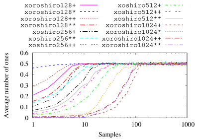
Figure 7. Convergence to “half of the bits are ones in average” plot.

9. A theoretical analysis of scramblers

We conclude the paper by discussing our scramblers from a theoretical point of view. We cast our discussion in the same theoretical framework as that of filtered linear-feedback shift registers. A filtered LFSR is given by an underlying LFSR and by a Boolean function that is applied to the state of the register. The final output is the output of the Boolean function. If the LFSR updates one bit at a time, we can see the Boolean function as sliding on the sequence of bits generated by the LFSR, emitting a scrambled output. The purpose of filtering a LFSR is that of making it more difficult to guess its next bit: the analogy with linear engines and scramblers is evident, as every scrambler can be seen as a set of $w$ boolean functions applied to the state of the linear engine. There are however a few differences:

• we use only primitive polynomials;

• we use several Boolean functions, and we are concerned with the behavior of their combined outputs;

• we do not apply a Boolean function to a sliding window of the same LFSR: rather, we have $kw$ copies of the same LFSR whose state is different, and we apply our set of Boolean functions to their single-bit output concatenated;

• we are not free to design our favorite Boolean functions: we are restricted to the ones computable with few arithmetic and logical operations;

• we are not concerned with predictability in the cryptographic sense, but just in the elimination of linear artifacts, that is, failures in tests for binary rank, linear complexity, and Hamming-weight dependencies.

We will see that many basic techniques coming from the cryptographic analysis of filtered LFSRs can be put to good use in our case. We will bring along a very simple example: a full-period xorshift linear engine with $w=3$ and $6$ bits of state (Vigna, 2016a). Its parameters are $a=1$ (left shift), $b=2$ (right shift), $c=1$ (right shift), and its characteristic polynomial is $p(x)=x^{6}+x^{5}+x^{3}+x^{2}+1$.

9.1. Representation by generating functions

We know that all bits of a linear engine satisfy linear recurrences with the same characteristic polynomial, but we can be more precise: we can fix a nonzero initial state and compute for each bit the generating function associated with the bit (see (Klein, 2013) for a detailed algorithm). Such functions have at the denominator the reciprocal polynomial $x^{n}p(1/x^{n})$ ($n$ here is the degree of $p$), whereas the numerator (a polynomial of degree less than $n$) represents the initial state. In our example, representing the first word using $x_{0}$ (lowest bit), $x_{1}$, $x_{2}$, the second word using $y_{0}$, $y_{1}$ and $y_{2}$, and using as initial state all bits set to zero except for $x_{0}$, we have

$$F_{x_{0}}(z) =\frac{z^{5}+z^{2}+z+1}{z^{6}+z^{4}+z^{3}+z+1} F_{y_{0}}(z) =\frac{z^{5}+z^{4}+z^{3}+z^{2}+z}{z^{6}+z^{4}+z^{3}+z+1}$$

$$F_{x_{1}}(z) =\frac{z^{5}+z^{2}}{z^{6}+z^{4}+z^{3}+z+1} F_{y_{1}}(z) =\frac{z^{4}+z}{z^{6}+z^{4}+z^{3}+z+1}$$

$$F_{x_{2}}(z) =\frac{z^{5}+z^{4}}{z^{6}+z^{4}+z^{3}+z+1} F_{y_{2}}(z) =\frac{z^{4}+z^{3}}{z^{6}+z^{4}+z^{3}+z+1}$$

If we write the formal series associated with each function, the $i$-th coefficient will give exactly the $i$-th output of the corresponding bit of the linear engine.

The interest in the representation by generating function lies in the fact that now we can perform some operations on the bits. For example, to study the lower bits of a generator using the $+$ scrambler to our linear engine, we add two bits, and we can easily compute the associated function, as adding coefficients is the same as adding functions:

$$F_{x_{0}+y_{0}}(z)=F_{x_{0}}(z)+F_{y_{0}}(z)\\ =\frac{z^{5}+z^{2}+z+1}{z^{6}+z^{4}+z^{3}+z+1}+\frac{z^{5}+z^{4}+z^{3}+z^{2}+z}{z^{6}+z^{4}+z^{3}+z+1}=\frac{z^{4}+z^{3}+1}{z^{6}+z^{4}+z^{3}+z+1}.$$

However, we are now stuck, because addition over $\mathbf{Z}/2^{w}\mathbf{Z}$ needs more than just xors. With ${x}_{0}$, ${x}_{1}$, $\dots\,$, ${x}_{w-1}$ and ${y}_{0}$, ${y}_{1}$, $\dots\,$, ${y}_{w-1}$ representing the bits, from least significant to most significant, of two $w$-bit words, to represent their arithmetic sum over $\mathbf{Z}/2^{w}\mathbf{Z}$ we can define the result bits $s_{i}$ and the carry bits $c_{i}$ using the recurrence

(8) $$s_{i} =x_{i}+y_{i}+c_{i-1}$$

(9) $$c_{i} =(x_{i}+y_{i})c_{i-1}+x_{i}y_{i}$$

where $c_{-1}=0$. This recurrence is fundamental because carries are the only source of nonlinearity in our scramblers (even multiplication by a constant can be turned into a series of shifts and sums). It is clear that to continue to the higher bits we need to be able to multiply two sequences, but multiplying generating functions, unfortunately, corresponds to a convolution of coefficients.

9.2. Representation in the splitting field

We now start to use the fact that the characteristic polynomial of our linear engine is primitive. Let $\mathbf{E}$ be the splitting field of a primitive polynomial $p(-)$ of degree $n$ over $\mathbf{Z}/2\mathbf{Z}$ (Lidl and Niederreiter, 1994). In particular, $\mathbf{E}$ can be represented as $(\mathbf{Z}/2\mathbf{Z})[\alpha]/p(\alpha)$, that is, by polynomials in $\alpha$ computed modulo $p(\alpha)$, and in that case by primitivity the zeroes of $p(-)$ are exactly the powers

$$\alpha,\alpha^{2},\alpha^{4},\alpha^{8},\ldots,\alpha^{2^{n-1}},$$

that is, the powers having exponents in the cyclotomic coset $C=\bigl{\{}\,1,2,4,8,\ldots,2^{n-1}\,\bigr{\}}$. Note that $\alpha^{2^{n}}=\alpha$ in $\mathbf{E}$. Every rational function $f(z)$ representing the output of a bit of the linear engine can then be expressed as a sum of partial fractions

(10) $$f(z)=\sum_{c\in C}\frac{\beta_{c}}{1-z\alpha^{c}},$$

where $\beta_{i}\in\mathbf{E}$, $\beta_{c}\neq 0$. As a consequence (Klein, 2013), the $j$-th bit $b_{j}$ of the sequence associated with $f(z)$ has an explicit description:

(11) $$b_{j}=\sum_{c\in C}\beta_{c}\bigl{(}\alpha^{c}\bigr{)}^{j}.$$

This property makes it possible to compute the sum of two sequences and the (output-by-output) product of two sequences. We just need to compute the sum or the product of the representation (11). The sum of two sequences is just a term-by-term sum, whereas in the case of a product we obtain a convolution. In both cases, we might experience cancellation—some of the $\beta$’s might become zero. But, whichever operation we apply, we will obtain in the end for a suitable set $S\subseteq[2^{n}]$ a representation of the form

(12) $$\sum_{c\in S}\beta_{c}\alpha^{c}.$$

with $\beta_{c}\neq 0$. The cardinality of $S$ is now exactly the degree of the polynomial at the denominator of the rational function

$$g(z)=\sum_{c\in S}\frac{\beta_{c}}{1-z\alpha^{c}}$$

associated with the new sequence, that is, its linear complexity (Klein, 2013). In our example, the coefficients of the representation (11) of $x_{0}$ are

$$\beta_{1} =\alpha^{4}+\alpha^{3} \beta_{8} =\alpha^{4}+\alpha^{3}+\alpha^{2}+\alpha$$

$$\beta_{2} =\alpha^{5}+\alpha^{3}+\alpha^{2}+\alpha \beta_{16} =\alpha^{5}+\alpha^{4}+\alpha^{3}+\alpha$$

$$\beta_{4} =\alpha^{5}+\alpha^{4}+\alpha^{2}+1 \beta_{32} =\alpha^{5}+\alpha^{2}+a$$

and similar descriptions are available for the other bits, so we are finally in the position of computing exactly the values of the recurrence (8): we simply have to use the representation in the splitting field to obtain a representation of $s_{i}$, and then revert to functional form using (10).

$$F_{s_{0}}(z) =\frac{z^{4}+z^{3}+1}{z^{6}+z^{4}+z^{3}+z+1}$$

$$F_{s_{1}}(z) =\frac{z^{13}+z^{9}+z^{8}+z}{z^{15}+z^{14}+z^{11}+z^{7}+z^{4}+z^{3}+1}$$

$$F_{s_{2}}(z) =\frac{z^{37}+z^{35}+z^{32}+z^{30}+z^{27}+z^{25}+z^{24}+z^{20}+z^{19}+z^{17}+z^{14}+z^{11}+z^{8}+z^{2}}{z^{41}+z^{39}+z^{34}+z^{32}+z^{30}+z^{28}+z^{27}+z^{26}+z^{24}+z^{23}+z^{17}+z^{16}+z^{15}+z^{14}+z^{13}+z^{11}+z^{9}+z^{8}+z^{7}+z^{6}+z^{5}+z^{3}+1}$$

Figure 8. The generating functions of the three bits of the xorshift+ generator.

The result is shown in Figure 8: as it is easy to see, we can still express the bits of xorshift+ as LFSRs, but their linear complexity rises quickly (remember that every generator with $n$ bits of state is a linear generator of degree $2^{n}$ with characteristic polynomial $x^{2^{n}}+1$, so “linear” should always mean “linear of low degree”).

Note that the generating function is irrelevant for our purposes: the only relevant fact is that the representation in the splitting field of the first bit has $6$ coefficients, that of the second bit $15$ and that of the third bit $41$, because, as we have already observed, these numbers are equal to the linear complexity of the bits of our xorshift+ generator. Unfortunately, this approach can be applied only to state arrays of less than a dozen bits: as the linear complexity increases due to the influence of carries, the number of terms in the representation (12) grows quickly, up to being unmanageable. Thus, this approach is limited to the analysis of small examples or the construction of counterexamples.

9.3. Representing scramblers by polynomials

A less exact but more practical approach to the analysis of the scrambled output of a generator is that of studying the scrambler in isolation. To do so, we are going to follow the practice of the theory of filtered LFSRs: we will represent the scramblers as a sum of Zhegalkin polynomials, that is, squarefree polynomials over $\mathbf{Z}/2\mathbf{Z}$. Due to the peculiarity of the field, no coefficients or exponents are necessary. If we can describe the function as a sum of distinct polynomials, we will say that the function is in algebraic normal form (ANF). For example, the $3$-bit scrambler of our example generator can be described by expanding recurrence (8) into the following three functions in ANF:

$$S_{0}(x_{0},x_{1},x_{2},y_{0},y_{1},y_{2}) =x_{0}+y_{0}$$

$$S_{1}(x_{0},x_{1},x_{2},y_{0},y_{1},y_{2}) =x_{1}+y_{1}+x_{0}y_{0}$$

$$S_{2}(x_{0},x_{1},x_{2},y_{0},y_{1},y_{2}) =x_{2}+y_{2}+x_{1}y_{1}+x_{0}y_{0}x_{1}+x_{0}y_{0}y_{1}$$

There is indeed a connection between the polynomial degree of a Boolean function, that is, the maximum degree of a polynomial in its ANF, the linear complexity of the bits of a linear engine, and the linear complexity of the bit returned by the Boolean function applied to the engine state. We will use the standard notation $[n]=\{\mskip 1.5mu0,1,2,\ldots,n-1\mskip 1.5mu\}$.

Lemma 9.1.

Let $\mathbf{E}$ be the splitting field of a primitive polynomial $p(x)$ of degree $n$, represented by polynomials in $\alpha$ computed modulo $p(\alpha)$. Then, there is a tuple $\langle t_{0},t_{1},\ldots t_{k-1}\rangle\in[n]^{k}$ such that

$$\prod_{i\in[k]}\alpha^{2^{t_{i}}}=\alpha^{c}$$

iff there is an $S\subseteq[n]$ with $0<|S|\leq k$ and

$$c=\sum_{s\in S}2^{s}.$$

Proof.

First we show that the all $c$’s are of the form above. When all the $t_{i}$’s are distinct, we have trivially $S=\{\mskip 1.5mut_{i}\mid 0\leq i<k\mskip 1.5mu\}$. If $t_{i}=t_{j}$

$$\alpha^{2^{t_{i}}}\alpha^{2^{t_{j}}}=\alpha^{2\cdot 2^{t_{i}}}=\alpha^{2^{t_{i}+1}},$$

remembering that computations of exponents of $\alpha$ are to be made modulo $2^{n}-1$. Thus, the problem is now reduced to a smaller tuple, and we can argue by induction that the result will be true of some $S\subseteq[k-1]\subseteq[k]$.

Now we show that for every $S$ as in the statement there exists a corresponding tuple. If $|S|=k$, this is obvious. Otherwise, let $|S|=j$ and ${s}_{0}$, ${s}_{1}$, $\dots\,$, ${s}_{j-1}$ be an enumeration of the elements of $S$. Then, the $k$-tuple

$$s_{0},s_{1},\ldots,s_{j-2},s_{j-1}-1,s_{j-1}-2,\ldots,s_{j-1}-k+j+1,s_{j-1}-k+j,s_{j-1}-k+j,$$

where the operations above are modulo $n$, gives rise exactly to the set $S$, as

$$\alpha^{2^{s_{j-1}-1}}\alpha^{2^{s_{j-1}-2}}\cdots\alpha^{2^{s_{j-1}-k+j+1}}\alpha^{2^{s_{j-1}-k+j}}\alpha^{2^{s_{j-1}-k+j}}=\alpha^{2^{s_{j}}}.$$

∎

An immediate consequence of the previous lemma is that there is a bound on the increase of linear complexity that a Boolean function, and thus a scrambler, can induce:

Proposition 9.2.

If $f$ is a Boolean function of $n$ variables with polynomial degree $d$ in ANF and $x_{i}$, $0\leq i<n$, are the bits of a linear engine with $n$ bits of state, then the rational function representing $f\bigl{(}x_{0},x_{1},\ldots,x_{n-1})$ has linear complexity at most

(13) $$U(n,d)=\sum_{j=1}^{d}{n\choose j}.$$

The result is obvious, as the number of possible nonzero coefficients of the splitting-field representation of $f\bigl{(}x_{0},x_{1}\dots,x_{n-1}\bigr{)}$ is bounded by $U(n,d)$ by Lemma 9.1. Indeed, $U(n,d)$ is well known: it is the standard bound on the linear complexity of a filtered LFSR. Our case is different, as we are applying Boolean functions to bits coming from different instances of the same LFSR, but the mathematics is the same.

There is also another inherent limitation: a uniform scrambler on $m$ bits cannot have polynomial degree $m$:

Proposition 9.3.

Consider a vector of $n$ Boolean functions on $m$ variables such that the preimage of each vector of $n$ bits contains exactly $2^{m-n}$ vectors of $m$ bits. Then, no function in the vector can have the (only) monomial of degree $m$ in its ANF.

Proof.

Since the vector of functions maps the same number of input values to each output value, if we look at each bit and consider its value over all possible vectors of $m$ bits, it must be zero $2^{m-1}$ times, one $2^{m-1}$ times. But all monomials of degree less than $m$ evaluate to an even number of zeroes and ones. The only monomial of degree $m$ evaluates to one exactly once. Hence, it cannot appear in any of the polynomial functions. ∎

Getting back to our example, the bounds for linear complexity of the bits of our xorshift+ generator are ${6\choose 1}=6$, ${6\choose 1}+{6\choose 2}=21$, and ${6\choose 1}+{6\choose 2}+{6\choose 3}=41$. From Figure 8, the first and last bits attain the upper bound (13), whereas the intermediate bit does not. However, Lemma 9.1 implies that every subset of $S$ might be associated with a nonzero coefficient. If this does not happen, as in the case of the intermediate bit, it must be the case that all the contributions for that subset of $S$ canceled out.

The amount of cancellation happening for a specific combination of linear engine and scrambler can in principle be computed exactly using the splitting-field representation, but as we have discussed this approach does not lend itself to computations beyond very small generators. However, we gathered some empirical evidence by computing the polynomial degree of the Boolean function associated with a bit using (8) and then by measuring directly the linear complexity using the Berlekamp–Massey algorithm (Klein, 2013): with careful implementation, this technique can be applied much beyond where the splitting-field representation can get. The algorithm needs an upper bound on the linear complexity to return a reliable result, but we have (13). We ran extensive tests on several generators, the largest being $12$-bit generators with $24$ bits of state. The results are quite uniform: unless the state array of the linear engine is tiny, if the characteristic polynomial is primitive, cancellation is an extremely rare event.

These empirical finds suggest that it is a good idea to independently study scramblers as Boolean functions, and in particular estimating or computing their polynomial degree. Then, given a class of generator, one should gather some empirical evidence that cancellation is rare, and at that point use the upper bound (13) as an estimate of linear complexity. This is the approach that we will follow in the following sections.

We remark however that a high polynomial degree is not sufficient to guarantee to pass all tests related to linearity. The problem is that such tests depend on the joint output of the Boolean functions we are considering. Moreover, there is a great difference between having a high polynomial degree and passing a linear-complexity or binary-rank test.

For example, consider the following pathological Boolean function that could be part of a scrambler:

(14) $$x_{w-1}+\prod_{i\in[w-1]}x_{i}.$$

This function has very high polynomial degree, and thus a likely high linear complexity. The problem is that if, say, $w=64$ from a practical viewpoint it is indistinguishable from $x_{w-1}$, as the “correction” that raises its linear complexity rarely happens. If the state array is small, this bit will fail all linearity tests. A single high-degree monomial is not sufficient in isolation, despite Lemma 9.1, so we will look for scramblers represented by a large number of monomials.

As a last counterexample, and cautionary tale, we consider the scrambler given by a change of sign, that is, multiplication by the all-ones word. It is trivial to write this scrambler using negated variables, but when we expand it in ANF we get

(15) $$\bar{x}_{w-1}+\prod_{k\in[w-1]}\bar{x}_{k}=1+x_{w-1}+\prod_{k\in[w-1]}\bigl{(}1+x_{k})=1+x_{w-1}+\prod_{S\subseteq[w-1]}\prod_{k\in S}x_{k}.$$

In other words, the ANF contains all monomials formed with all other bits, but the Boolean function is still as pathological as (14), as there is no technical difference between $x_{i}$ and $\bar{x}_{i}$. Too few monomials are problematic, but too many are, too.

9.4. The + scrambler

We conclude this part of the paper with a detailed discussion of each scrambler, using their representations by squarefree polynomials, as discussed in the previous section. We start from the + scrambler, introduced in Section 4.1. Recurrence (8) can be easily unfolded to a closed form for the scrambled bit $s_{b}$:

(16) $$s_{b}=x_{b}+y_{b}+\sum_{i=1}^{b}x_{i-1}y_{i-1}\sum_{S\subseteq[b-i]}\prod_{j\in S}x_{i+j}\prod_{j\in[b-i]\setminus S}y_{i+j}\\ =x_{b}+y_{b}+\sum_{i=1}^{b}x_{i-1}y_{i-1}\prod_{j\in[b-i]}\bigl{(}x_{i+j}+y_{i+j}\bigr{)}.$$

If the $x_{i}$’s and the $y_{i}$’s are distinct, the expressions above are in ANF: there are exactly $2^{b}+1$ monomials with maximum degree $b+1$. Thus, if the underlying linear engine has $n$ bits of state the linear-degree bound for bit $b$ will be $U(n,b+1)$, where $U(-,-)$ is defined by (13).

An important observation is that no monomial appears in two instances of the formula for different values of $b$. This implies that any linear combination of bits output by the + scrambler has the same linear complexity as the bit of highest degree, and at least as many monomials: we say in this case that there is no polynomial degree loss. Thus, except for the very lowest bits, we expect that no linearity will be detectable.

In Table 11 we report, using (13), the estimated linear complexity of the lowest bits of some generators. The lowest values have also been verified using the Berlekamp–Massey algorithm: as expected, we could not detect any linear-degree loss; running the algorithm on the largest values is unfeasible. While an accurate linear-complexity test might catch the fourth lowest bit of xoroshiro128+, the degree raises quickly to the point the linearity is undetectable.

xoroshiro128+	xoshiro256+	xoshiro512+	xoroshiro1024+	xoroshiro64+	xoshiro128+
128	256	512	1024	64	128
8256	32896	131328	524800	2080	8256
349632	2796416	22370048	178957824	43744	349632
11017632	177589056	2852247168	45723987200	679120	11017632
275584032	8987138112	290367762560	9336909979904	8303632	275584032

Table 11. Estimated linear complexity of the five lowest bits of generators (the first line is bit 0) using the + scrambler.

The situation for Hamming-weight dependencies is not so good, however, as empirically (Table 1) we have already observed that xoroshiro engines still fail our test (albeit using three orders of magnitude more data). We believe that this is due to the excessively regular structure of the monomials.

Note that if the underlying linear engine is $d$-dimensionally equidistributed, the scrambler generator will be in general at most $(d-1)$-dimensionally equidistributed (see Section 7).

9.5. The * scrambler

We now discuss the * scrambler, introduced in Section 4.2, in the case of a multiplicative constant of the form $2^{s}+1$. This case is particularly interesting because it is very fast on recent hardware; in particular, $(2^{s}+1)\cdot x=x+(x\ll s)$, where the sum is in $\mathbf{Z}/2^{w}\mathbf{Z}$, which provides a multiplication-free implementation. Moreover, as we will see, the analysis of the $2^{s}+1$ case sheds light on the general case, too.

Let $z=(2^{s}+1)x$. Specializing (16), we have that $z_{b}=x_{b}$ when $b<s$; otherwise, $b=c+s\geq s$ and

(17) $$z_{b}=z_{c+s}=x_{c+s}+x_{c}+\sum_{i=1}^{c}x_{i-1+s}\,x_{i-1}\sum_{S\subseteq[c-i]}\prod_{j\in S}x_{i+j+s}\prod_{j\in[c-i]\setminus S}x_{i+j}\\ =x_{c+s}+x_{c}+\sum_{i=1}^{c}x_{i-1+s}\,x_{i-1}\prod_{k\in[c-i]}\bigl{(}x_{i+k+s}+x_{i+k}\bigr{)}.$$

However, contrarily to (16) the expressions above do not denote an ANF, as the same variable may appear many times in the same monomial.

We note that the monomial $x_{s}x_{0}x_{s+1}\cdots x_{s+c-1}$, which is of degree $c+1$, appears only and always in the function associated with $y_{b}$, $b>s$. Thus, bits with $b\leq s$ have degree one, whereas bits $b$ with $b>s$ have degree $b-s+1$. In particular, as in the case of +, there is no polynomial degree loss when combining different bits.

In the case of a generic (odd) constant $m$, one has to modify recurrence (8) to start including shifted bits at the right stage, which creates a very complex monomial structure. Note, however, that bits after the second-lowest bit set in $m$ cannot modify the polynomial degree. Thus, the decrease of Hamming-weight dependencies we observe in Table 1 even for xoroshiro* is not due to a higher polynomial degree with respect to + (indeed, the opposite is true), but to a richer structure of the monomials. The degree reported for the + scrambler in Table 11 can indeed be adapted to the present case: one has just to copy the first line as many times as the index of the second-lowest bit set in $m$.

To get some intuition about the monomial structure, it is instructive to get back to the simpler case $m=2^{s}+1$. From (17) it is evident that monomials associated with different values of $i$ cannot be equal, as the minimum variable appearing in a monomial is $x_{i-1}$. Once we fix $i$ with $1\leq i\leq c$, the number of monomials is equal to the number of sets of the form

(18) $$S+s\;\cup\;[c-i]\setminus S\;\cup\;\left\{\mskip 1.5mus-1\mskip 1.5mu\right\}\qquad S\subseteq[c-i]$$

that can be expressed by an odd number of values of $S$ (if you can express the set in an even number of ways, they cancel out). But such sets are in bijection with the values $(v\ll s)\lor\lnot v\lor(1\ll s-1)$ as $v$ varies among the words of $c-i$ bits. In a picture, we are looking at the columnwise logical or of the following diagram, where the $b_{j}$’s are the bits of $v$, for convenience numbered from the most significant:

The first obvious observation is that if $s>c-i$ the two rows are nonoverlapping, and they are not influenced by the one in position $s-1$. In this case, we obtain all possible $2^{c-i}$ monomials. More generally, such sets are all distinct iff $s\geq(c-i+1)/2$, as in that case the values must differ either in the first $s$ or in the last $s-1$ bits: consequently, the number of monomials, in this case, is again $2^{c-i}$. Minimizing $i$ and maximizing $c$ we obtain $s\geq(w-s-1)/2$, whence $s\geq(w-1)/3$. In this case, the monomials of $z_{b}$ are exactly $2+2^{c-1}+2^{c-2}+\cdots+1=2^{c}+1=2^{b-s}+1$ when $b\geq s$.

As $s$ moves down from $(w-1)/3$, we observe empirically more and more reduction in the number of monomials with respect to the maximum possible $2^{b-s}+1$. When we reach $s=1$, however, a radical change happens: the number of monomials grows as $2^{b/2}$.

Theorem 9.4.

The number of monomials of the Boolean function representing bit $b$ of $3x$ is

$$(2+[\text{$b$ odd}])\cdot 2^{\lfloor b/2\rfloor}-1.$$

We remark a surprising combinatorial connection: this is the number of binary palindromes smaller than $2^{b}$, that is, A052955 in the “On-Line Encyclopedia of Integer Sequences” (Inc., 2017).

Proof.

When $s=1$, the different subsets in (18) obtained when $S$ varies are in bijection with the values $v\lor\lnot(v\gg 1)$ as $v$ varies among the words of $c-i$ bits. Again, we are looking at the logical or by columns of the following diagram, where the $b_{j}$’s are the bits of $v$ numbered from the most significant:

Note that if there is a $b_{j}$ whose value is irrelevant, flipping will generate two monomials that will cancel each other.

Let us consider now a successive assignment of values to the $b_{j}$’s, starting from $b_{0}$. We remark that as long as we assign ones, no assigned bit is irrelevant. As soon as we assign a zero, however, say to $b_{j}$, we have that the value of $b_{j+1}$ will no longer be relevant. To make $b_{j+1}$ relevant, we need to set $b_{j+2}=0$. The argument continues until the end of the word, so we can actually choose the value of $(c-i-j-1)/2$ bits, and only if $c-i-j-1$ is even (otherwise, $b_{c-i-1}$ has no influence).

We now note that if we flip a bit $b_{k}$ that we were forced to set to zero, there are two possibilities: either we chose $b_{k-1}=1$, in which case we obtain a different monomial, or we chose $b_{k-1}=0$, in which case $b_{k}$ is irrelevant, but by flipping also $b_{k+1}$ we obtain once again the same monomial, so the two copies cancel each other.

Said otherwise, monomials with an odd number of occurrences are generated either when all bits of $v$ are set to one, or when there is a string of ones followed by a suffix of odd length in which every other bit (starting from the first one) is zero. All in all, we have

$$1+\sum_{k=0}^{\bigl{\lfloor}\frac{c-i-1}{2}\bigr{\rfloor}}2^{k}=2^{\bigl{\lceil}\frac{c-i-1}{2}\bigr{\rceil}}$$

possible monomials, where $2k+1$ is the length of the suffix. Adding up over all $i$’s, and adding the two degree-one monomials we have that the number of monomials of $y_{b}$ for $b=c+1>0$ is

$$2+\sum_{i=1}^{b-1}2^{\bigl{\lceil}\frac{b-i-2}{2}\bigr{\rceil}}=1+1+\sum_{i=1}^{b-1}2^{\bigl{\lceil}\frac{b-i-2}{2}\bigr{\rceil}}=(2+[\text{$b$ odd}])\cdot 2^{\lfloor b/2\rfloor}-1.$$

The correctness for the case $b=0$ can be checked directly. ∎

We remark that in empirical tests the $3x$ scrambler performs very poorly: thus, the excessive cancellation of monomials implied by the theorem above has practical consequences.

9.6. The ++ scrambler

We will now examine the strong scrambler ++ introduced in Section 4.3. We choose two words $x$, $y$ from the state of the linear engine and then $z=\rho_{r}(x+y)+x$, where $+$ denotes sum in $\mathbf{Z}/2^{w}\mathbf{Z}$.

Computing an ANF for the final Boolean functions appears to be a hard combinatorial problem: nonetheless, with this setup we know that the lowest bit will have polynomial degree $w-r+1$, and we expect that the following bits will have an increasing degree, possibly up to saturation. Symbolic computations in low dimension show however that the growth is quite irregular. The linear complexity of the lowest bits is large, as shown in Table 12, where we display a theoretical estimate based on (13), assuming that on lower bits degree increase at least by one at each bit (experimentally, it usually grows more quickly—see again Table 12).

xoroshiro128++	xoshiro256++	xoshiro512++	xoroshiro1024++	xoshiro128++
$1\times 10^{36}$	$3\times 10^{48}$	$1\times 10^{68}$	$9\times 10^{74}$	$1\times 10^{27}$
$2\times 10^{36}$	$2\times 10^{49}$	$1\times 10^{69}$	$2\times 10^{76}$	$5\times 10^{27}$
$3\times 10^{36}$	$1\times 10^{50}$	$9\times 10^{69}$	$4\times 10^{77}$	$2\times 10^{28}$
$4\times 10^{36}$	$4\times 10^{50}$	$8\times 10^{70}$	$1\times 10^{79}$	$6\times 10^{28}$

Table 12. Approximate lower bound on the estimated linear complexity of the four lowest bits (the first line is bit 0) of generators using the ++ scrambler with parameters from Table 3 and 6.

This scrambler is potentially very fast, as it requires just three operations and no multiplication, and it can reach a high polynomial degree, as it uses $2w$ bits. Moreover, its simpler structure makes it attractive in hardware implementations. However, the very regular structure of the + scrambler makes experimentally ++ less effective on Hamming-weight dependencies.

As a basic heuristic, we suggest to choose a rotation parameter $r\in[w/4\,\mathpunct{\ldotp\ldotp}3w/4]$ such that $r$ and $w-r$ are both prime (or at least odd), and they are not equal to any of the shift/rotate parameters appearing in the generator (the second condition being more relevant than the first one). Smaller values of $r$ will of course provide a higher polynomial degree, but too small values yield too short carry chains. For $w=64$ candidates are $17$, $23$, $41$, and $47$; for $w=32$ one has $13$ and $19$; for $w=16$ one has $5$ and $11$. In any case, a specific combination of linear engine and scrambler should be tested thoroughly.

As in the case of the + scrambler, if the underlying linear engine is $d$-dimensionally equidistributed, the scrambler generator will be in general at most $(d-1)$-dimensionally equidistributed (see Section 7).

9.7. The ** scrambler

We conclude our discussion with the strong scrambler ** introduced in Section 4.4. We will be discussing in detail the case with multiplicative constants of the form $2^{s}+1$ and $2^{t}+1$, which is particularly fast (the $+$ symbol will denote sum in $\mathbf{Z}/2^{w}\mathbf{Z}$ for the rest of this section).

Let $z=\rho_{r}(x\cdot(2^{s}+1))\cdot(2^{t}+1)$. The $\min\{\mskip 1.5mur,t\mskip 1.5mu\}$ lowest bits of $z$ are the $\min\{\mskip 1.5mur,t\mskip 1.5mu\}$ highest bits of $x\cdot(2^{s}+1)$. To choose $s$, $r$, and $t$ we can leverage our previous knowledge of the scrambler *. We start by imposing that $s<t$, as choosing $s=t$ generates several duplicates that reduce significantly the number of monomials in the ANF of the final Boolean functions, whereas $t<s$ provably yields a lower minimum degree for the same $r$ (empirical computations show also a smaller number of monomials). We also have to impose $t<r$, for otherwise some bits or xor of pair of bits will have very low linear complexity (polynomial degree one). So we have to choose our parameters with the constraint $s<t<r$. Since the degree of the lowest bit is $\max(1,w-r-s+1)$, choosing $r=t+1$ maximizes the minimum degree across the bits. Moreover, we would like to keep $s$ and $t$ as small as possible, to increase the minimum linear complexity and also to make the scrambler faster.

Also in this case computing an ANF for the final Boolean functions appears to be a hard combinatorial problem: nonetheless, with this setup we know that the lowest bit will have (when $r+s\leq w$) polynomial degree $w-r-s+1$, and we expect that the following bits will have increasing degree up to saturation (which happens at degree $w-1$ by Proposition 9.3). Symbolic computations in low dimension show some polynomial degree loss caused by the second multiplication unless $r=2t+1$; moreover, for that value of $r$ the polynomial degree loss when combining bits is almost absent. Taking into consideration the bad behavior of the multiplier $3$ highlighted by Theorem 9.4, we conclude that the best choice is $s=2$, $t=3$, and consequently $r=7$. These are the parameters reported in Table 3. The linear complexity of the lowest bits is extremely large, as shown in Table 13.

xoroshiro128**	xoshiro256**	xoshiro512**	xoroshiro1024**	xoroshiro64**	xoshiro128**
$3\times 10^{37}$	$2\times 10^{57}$	$4\times 10^{75}$	$1\times 10^{93}$	$2\times 10^{18}$	$8\times 10^{25}$
$4\times 10^{37}$	$7\times 10^{57}$	$3\times 10^{76}$	$2\times 10^{94}$	$3\times 10^{18}$	$3\times 10^{26}$
$6\times 10^{37}$	$3\times 10^{58}$	$2\times 10^{77}$	$3\times 10^{95}$	$5\times 10^{18}$	$1\times 10^{27}$
$7\times 10^{37}$	$9\times 10^{58}$	$2\times 10^{78}$	$6\times 10^{96}$	$6\times 10^{18}$	$5\times 10^{27}$

Table 13. Approximate estimated linear complexity of the four lowest bit (the first line is bit 0) of generators using the ** scrambler with parameters from Table 3 and 6.

At $32$ bits, however, tests show that this scrambler is not sufficiently powerful for xoroshiro64, and Table 6 reports indeed different parameters: the first multiplier is the constant used for the * scrambler, and the second multiplier $2^{t}+1$ has been chosen so that bit $t$ is not set in the first constant. Again, $r=2t+1$, following the same heuristic of the previous case.

10. Conclusions

The combination of xoroshiro/xoshiro and suitable scramblers provides a wide range of high-quality and fast solutions for pseudorandom number generation. Parallax has embedded in their recently designed Propeller 2 microcontroller xoroshiro128** and the $16$-bit xoroshiro32++; xoroshiro116+ is the stock generator of Erlang and xoshiro256** is the stock generator of the popular embedded language Lua and of GNU Fortran. xoroshiro128++ and xoshiro256++ are scheduled to be included in Java 17 as part of JDK Enhancement Proposal 356. Recently, the speed of xoshiro128** has found application in cryptography (Bos et al., 2018; Gérard and Rossi, 2019).

We believe that a more complete study of scramblers can shed some further light on the behavior of such generators: the open problem is that of devising a model explaining the elimination of Hamming-weight dependencies. The main difficulty is that analyzing the Boolean functions representing each scrambled bit in isolation is not sufficient, as Hamming-weight dependencies are generated by their collective behavior.

There are variants of the scramblers we discussed that do not use rotations: for example, in the ++ and ** scramblers the rotation can be replaced by xoring $x$ with $x\gg r$, as also this operation will increase the linear complexity of the lower bits. For contexts in which rotations are not available or too expensive, one might explore the possibility of using xorshift generators scrambled with such variants.

There is a vast literature on filtered LFSR that might be used to prove aspects we approached only with symbolic small-state computations. For example, in (Kolokotronis et al., 2007) the authors prove a lower bound on the linear degree of a Boolean function made of a single very specific monomial, something for which we just argued based on measurements made using the Berlekamp–Massey algorithm. In (Braeken and Semaev, 2005) the authors try to provide closed forms or even ANFs when the argument of a Boolean function is multiplied or summed with a constant, which might be a starting point for a closed form for the ** scrambler.

In general, it is an interesting open problem to correlate explicitly the monomial structure of a Boolean function in ANF with its resilience to linearity tests. Intuitively, recalling (15), one sees that besides large-degree monomials one needs small-degree monomials to make the tests “perceive” the increase in linear complexity at the right time.

- (1)
- Blackman and Vigna (2020) David Blackman and Sebastiano Vigna. 2020. A New Test for Hamming-Weight Dependencies. (2020).
- Bos et al. (2018) Joppe W. Bos, Simon Friedberger, Marco Martinoli, Elisabeth Oswald, and Martijn Stam. 2018. Fly, you fool! Faster Frodo for the ARM Cortex-M4. Cryptology ePrint Archive, Report 2018/1116. (2018). https://eprint.iacr.org/2018/1116.
- Bourbaki (1989) Nicolas Bourbaki. 1989. Algebra: Elements of Mathematics. Springer-Verlag.
- Braeken and Semaev (2005) An Braeken and Igor A. Semaev. 2005. The ANF of the Composition of Addition and Multiplication mod with a Boolean Function. In Fast Software Encryption: 12th International Workshop, FSE 2005, Paris, France, February 21-23, 2005, Revised Selected Papers (Lecture Notes in Computer Science), Henri Gilbert and Helena Handschuh (Eds.), Vol. 3557. Springer, 112–125.
- Caracciolo et al. (2009) Sergio Caracciolo, Alan D. Sokal, and Andrea Sportiello. 2009. Noncommutative determinants, Cauchy–Binet formulae, and Capelli-type identities I. Generalizations of the Capelli and Turnbull identities. The Electronic Journal of Combinatorics 16, 1 (2009), 103.
- Carter (1989) G. D. Carter. 1989. Aspects of local linear complexity. Ph.D. Dissertation. University of London.
- Chervov et al. (2009) A. Chervov, G. Falqui, and V. Rubtsov. 2009. Algebraic properties of Manin matrices 1. Advances in Applied Mathematics 43, 3 (2009), 239–315.
- Compagner (1991) Aaldert Compagner. 1991. The hierarchy of correlations in random binary sequences. Journal of Statistical Physics 63, 5-6 (1991), 883–896.
- Erdmann (1992) E. D. Erdmann. 1992. Empirical tests of binary keystreams. (1992).
- Gérard and Rossi (2019) François Gérard and Mélissa Rossi. 2019. An Efficient and Provable Masked Implementation of qTESLA. Cryptology ePrint Archive, Report 2019/606. (2019). https://eprint.iacr.org/2019/606.
- Haramoto et al. (2008) Hiroshi Haramoto, Makoto Matsumoto, Takuji Nishimura, François Panneton, and Pierre L’Ecuyer. 2008. Efficient Jump Ahead for -Linear Random Number Generators. INFORMS Journal on Computing 20, 3 (2008), 385–390.
- Inc. (2017) OEIS Foundation Inc. 2017. The On-Line Encyclopedia of Integer Sequences. (2017). http://oeis.org/
- Klein (2013) Andreas Klein. 2013. Stream Ciphers. Springer London, London.
- Knuth (1992) Donald E. Knuth. 1992. Two notes on notation. American Mathematical Monthly 99, 5 (May 1992), 403–422.
- Knuth (1997) Donald E. Knuth. 1997. The Art of Computer Programming, Volume 1, Fundamental Algorithms (third ed.). Addison-Wesley, Reading, MA, USA. xix+650 pages.
- Kolokotronis et al. (2007) Nicholas Kolokotronis, Konstantinos Limniotis, and Nicholas Kalouptsidis. 2007. Improved Bounds on the Linear Complexity of Keystreams Obtained by Filter Generators. In Inscrypt (Lecture Notes in Computer Science), Dingyi Pei, Moti Yung, Dongdai Lin, and Chuankun Wu (Eds.), Vol. 4990. Springer, 246–255.
- L’Ecuyer (1996) Pierre L’Ecuyer. 1996. Maximally Equidistributed Combined Tausworthe Generators. Math. Comp. 64, 213 (1996), 203–213.
- L’Ecuyer and Granger-Piché (2003) Pierre L’Ecuyer and Jacinthe Granger-Piché. 2003. Combined generators with components from different families. Mathematics and Computers in Simulation 62, 3 (2003), 395–404. 3rd IMACS Seminar on Monte Carlo Methods.
- L’Ecuyer and Panneton (2005) Pierre L’Ecuyer and François Panneton. 2005. Fast random number generators based on linear recurrences modulo 2: overview and comparison. In Proceedings the the 2005 Winter Simulation Conference. IEEE, 110–119.
- L’Ecuyer and Panneton (2009) Pierre L’Ecuyer and François Panneton. 2009. -Linear Random Number Generators. In Advancing the Frontiers of Simulation, Christos Alexopoulos, David Goldsman, and James R. Wilson (Eds.). International Series in Operations Research & Management Science, Vol. 133. Springer US, 169–193.
- L’Ecuyer and Simard (2007) Pierre L’Ecuyer and Richard Simard. 2007. TestU01: A C library for empirical testing of random number generators. ACM Trans. Math. Softw. 33, 4, Article 22 (2007).
- Lewis (2018) Robert H. Lewis. 2018. Fermat: A Computer Algebra System for Polynomial and Matrix Computation. (2018). http://home.bway.net/lewis/
- Lidl and Niederreiter (1994) Rudolf Lidl and Harald Niederreiter. 1994. Introduction to finite fields and their applications. Cambridge University Press, Cambridge.
- Marsaglia (2003) George Marsaglia. 2003. Xorshift RNGs. Journal of Statistical Software 8, 14 (2003), 1–6.
- Marsaglia and Tsay (1985) George Marsaglia and Liang-Huei Tsay. 1985. Matrices and the structure of random number sequences. Linear Algebra Appl. 67 (1985), 147–156.
- Matsumoto and Nishimura (1998) Makoto Matsumoto and Takuji Nishimura. 1998. Mersenne Twister: A 623-Dimensionally Equidistributed Uniform Pseudo-Random Number Generator. ACM Trans. Model. Comput. Simul. 8, 1 (1998), 3–30.
- Matsumoto et al. (2007) Makoto Matsumoto, Isaku Wada, Ai Kuramoto, and Hyo Ashihara. 2007. Common Defects in Initialization of Pseudorandom Number Generators. ACM Trans. Model. Comput. Simul. 17, 4 (2007).
- Naus (1968) Joseph I. Naus. 1968. An Extension of the Birthday Problem. The American Statistician 22, 1 (1968), 27–29.
- Niederreiter (1995) Harald Niederreiter. 1995. The multiple-recursive matrix method for pseudorandom number generation. Finite Fields and their Applications 1, 1 (1995), 3–30.
- Nishimura (2000) Takuji Nishimura. 2000. Tables of 64-bit Mersenne Twisters. ACM Transactions on Modeling and Computer Simulation (TOMACS) 10, 4 (2000), 348–357.
- Panneton et al. (2006) François Panneton, Pierre L’Ecuyer, and Makoto Matsumoto. 2006. Improved long-period generators based on linear recurrences modulo 2. ACM Trans. Math. Softw. 32, 1 (2006), 1–16.
- Saito and Matsumoto (2009) Mutsuo Saito and Makoto Matsumoto. 2009. A PRNG Specialized in Double Precision Floating Point Numbers Using an Affine Transition. In Monte Carlo and Quasi-Monte Carlo Methods 2008, Pierre L’Ecuyer and Art B. Owen (Eds.). Springer Berlin Heidelberg, 589–602. DOI:http://dx.doi.org/10.1007/978-3-642-04107-5_38
- Saito and Matsumoto (2014) Mutsuo Saito and Makoto Matsumoto. 2014. XSadd (Version 1.1). (25 March 2014). http://www.math.sci.hiroshima-u.ac.jp/~m-mat/MT/XSADD/
- Saito and Matsumoto (2015) Mutsuo Saito and Makoto Matsumoto. 2015. Tiny Mersenne Twister (Version 1.1). (24 March 2015). http://www.math.sci.hiroshima-u.ac.jp/~m-mat/MT/TINYMT/
- Sothanaphan (2017) Nat Sothanaphan. 2017. Determinants of block matrices with noncommuting blocks. Linear Algebra Appl. 512, Supplement C (2017), 202–218.
- Steele et al. (2014) Guy L. Steele, Jr., Doug Lea, and Christine H. Flood. 2014. Fast Splittable Pseudorandom Number Generators. In Proceedings of the 2014 ACM International Conference on Object Oriented Programming Systems Languages & Applications (OOPSLA ’14). ACM, New York, NY, USA, 453–472.
- Terpstra et al. (2010) Dan Terpstra, Heike Jagode, Haihang You, and Jack Dongarra. 2010. Collecting Performance Data with PAPI-C. In Tools for High Performance Computing 2009, Matthias S. Müller, Michael M. Resch, Alexander Schulz, and Wolfgang E. Nagel (Eds.). Springer Berlin Heidelberg, 157–173.
- The Sage Developers (2018) The Sage Developers. 2018. SageMath, the Sage Mathematics Software System (Version 8.0). http://www.sagemath.org
- Vigna (2016a) Sebastiano Vigna. 2016a. An experimental exploration of Marsaglia’s xorshift generators, scrambled. ACM Trans. Math. Software 42, 4, Article 30 (2016).
- Vigna (2016b) Sebastiano Vigna. 2016b. Further scramblings of Marsaglia’s xorshift generators. J. Comput. Appl. Math. 315 (2016), 175–181.
- Vigna (2019) Sebastiano Vigna. 2019. It is high time we let go of the Mersenne Twister. CoRR abs/1910.06437 (2019).
- Vigna (2020) Sebastiano Vigna. 2020. On the probability of overlap of random subsequences of pseudorandom number generators. Inform. Process. Lett. 158 (2020).