The $\bm{\Lambda_{b}\,\to}\bm{\Lambda\,(\to p\pi^{-})\mu^{+}\mu^{-}}$ decay in the $\text{RS}_{\bm{c}}$ model

Abstract

We study the four body decay $\Lambda_{b}\rightarrow\Lambda(\rightarrow p\pi^{-})\mu^{+}\mu^{-}$ in the Randall-Sundrum model with custodial protection $(\text{RS}_{c})$. By considering the constraints coming from the direct searches of the lightest Kaluza-Klein (KK) excitation of the gluon, electroweak precision tests, the measurements of the Higgs signal strengths at the LHC and from $\Delta F=2$ flavor observables, we perform a scan of the parameter space of the $\text{RS}_{c}$ model and obtain the maximum allowed deviations of the Wilson coefficients $\Delta C^{(\prime)}_{7,\;9,\;10}$ for different values of the lightest KK gluon mass $M_{g^{(1)}}$. Later, their implications on the observables such as differential branching fraction, longitudinal polarization of the daughter baryon $\Lambda$, forward-backward asymmetry with respect to leptonic, hadronic and combined lepton-hadron angles are discussed where we present the analysis of these observables in different bins of di-muon invariant mass squared $s\;(=q^{2})$. It is observed that with the current constraints the Wilson coefficients in $\text{RS}_{c}$ model show slight deviations from their Standard Model values and hence can not accommodate the discrepancies between the Standard Model calculations of various observables and the LHCb measurements in $\Lambda_{b}$ decays.

1 Introduction

Although the Large Hadron Collider (LHC) has so far not observed any new particles directly, that are predicted by many beyond Standard Model (SM) scenarios, it has certainly provided some intriguing discrepancies from the SM expectations in semi-leptonic rare $B$-meson decays. In this context, a persistent pattern of deviations in tension with the SM predictions has been emerging from observables in a number of $b\to sl^{+}l^{-}$ processes. In particular, LHCb measurements [1, 2] of the observables $R_{K}$ and $R_{K^{\ast}}$ representing the ratios of branching fractions $B^{+}\to K^{+}\mu^{+}\mu^{-}$ to $B^{+}\to K^{+}e^{+}e^{-}$ and $B^{0}\to K^{\ast 0}\mu^{+}\mu^{-}$ to $B^{0}\to K^{\ast 0}e^{+}e^{-}$, respectively, show deviations from the SM predictions $\sim 1$ and together they indicate the lepton flavor universality violation with the significance at the $4\sigma$ level [3, 4, 5, 6]. Further, the LHCb results for the branching fractions of the $B\to K^{(\ast)}\mu^{+}\mu^{-}$ and $B_{s}\to\phi\mu^{+}\mu^{-}$ decays [7, 8, 9], suggest the smaller values compared to their SM estimates. Moreover, mismatch between the LHCb findings and the SM predictions in the angular analysis of the $B^{0}\to K^{\ast 0}\mu^{+}\mu^{-}$ decay [10, 11], with the confirmation by the Belle collaboration later on [12], has become a longstanding issue. In this context, recent phenomenological analyses have explored the underlying new physics (NP) possibilities behind these anomalies [3, 4, 5, 6, 13, 14, 15, 16, 17, 18]. However, to establish the claim that the deviations in the angular asymmetries in $B\to K^{*}(\to K\pi)\mu^{+}\mu^{-}$ decays are indications of NP, an improvement is needed both on the theoretical and the experimental sides. On theoretical front we have to get better control on the hadronic uncertainties arising mainly due to form factors (FF) and on the experimental end, some more data with improved statistics is needed which is expected from the Belle II and LHCb. Another possibility that exist on the theoretical side is to analyze more processes which are mediated by the same quark level transition $b\to s\mu^{+}\mu^{-}$.

Among them, the rare baryonic decay $\Lambda_{b}\to\Lambda\mu^{+}\mu^{-}$ is particularly important as it can provide complementary information and additionally offers a unique opportunity to understand the helicity structure of the effective weak Hamiltonian for $b\to s$ transition [19, 20]. The branching ratio for this decay was first measured by CDF collaboration [21]. Recently, the LHCb has reported its measurements for branching ratio and three angular observables [22] in the $\Lambda_{b}\to\Lambda(\to p\pi^{-})\mu^{+}\mu^{-}$ decay. Theoretically challenging aspect in the study of the $\Lambda_{b}\to\Lambda\mu^{+}\mu^{-}$ decay is the evaluation of the hadronic $\Lambda_{b}\to\Lambda$ transition from factors. In this context, recent progress is made by performing the high precision lattice QCD calculations [23]. Moreover, these FF have been estimated using various models or approximations such as quark models [24, 25], perturbative QCD [26], SCET [27] and QCD light cone sum-rules (LCSR) [28, 29, 30]. Furthermore, extensive studies of the semi-leptonic decays of $\Lambda_{b}$ baryon $(\Lambda_{b}\to\Lambda\ell^{+}\ell^{-})$, both within the SM and in many different NP scenarios, have been performed [31, 32, 33, 34, 35, 36, 37, 38, 39, 40, 41, 42, 43, 44, 45, 46, 47, 48, 49, 50, 51, 52, 53, 54, 55, 56]. Recently, the angular distributions for polarized $\Lambda_{b}$ are presented in [57].

In the present work, we study the four body $\Lambda_{b}\to\Lambda(\to p\pi^{-})\mu^{+}\mu^{-}$ decay in the framework of the Randall-Sundrum (RS) model with custodial protection. The RS model features five-dimensional (5D) space-time with a non-trivial warped metric [58]. After performing the KK decomposition and integrating over the fifth dimension the effective 4D theory is obtained which involves new particles appearing as the KK resonances, either of the SM particles or the ones which do not possess SM counterparts. Assuming that the weak effective Hamiltonian of the $\Lambda_{b}\to\Lambda(\to p\pi^{-})\mu^{+}\mu^{-}$ decay emerges from the well-defined theory of the $\text{RS}_{c}$ model, the Wilson coefficients of the effective Hamiltonian get modified with respect to the SM values due to additional contributions from the heavy KK excitations and are correlated in a unique way. Expecting distinct phenomenological consequences from such a correlation on the angular observables of the $\Lambda_{b}\to\Lambda(\to p\pi^{-})\mu^{+}\mu^{-}$ decay, we study whether the current experimental data on this decay can be explained in the $\text{RS}_{c}$ model.

Although $B$-meson decays have been investigated extensively in different variants of the RS model [59, 60, 61, 62, 63, 64, 65, 66, 67, 68, 69, 70, 71, 72], not many studies are devoted to the $\Lambda_{b}$ decays in the RS model [73]. Additionally, our present study includes new considerations and results which were not available in the previous studies of the $\Lambda_{b}$ decays entertaining the RS model. Firstly, we will consider the current constraints on the parameter space of the $\text{RS}_{c}$ model coming from the direct searches of the lightest KK gluon, electroweak precision tests and from the measurements of the Higgs signal strengths at the LHC, which yield much stricter constraints on the mass scale of the lowest KK gluon $M_{g^{(1)}}$, which in turn prevent sizeable deviations of the Wilson coefficients from the SM predictions. Secondly, we will not adopt the simplification of treating the elements of the 5D Yukawa coupling matrices to be real numbers as considered in [73, 68], rather we will take these entries to be complex numbers as considered in [70, 63] leading to the complex Wilson coefficients instead of real ones. Last but not the least, we will use the helicity parametrization of the $\Lambda_{b}\to\Lambda$ hadronic matrix elements and for the involved FF, we will use the most recent lattice QCD calculations, both in the low and high $q^{2}$ regions, which yield much smaller uncertainties in most of the kinematic range [23].

The rest of the paper is organized as follows. In Sec. 2, we describe the essential features of the $\text{RS}_{c}$ model especially relevant for the study of the considered decay. In Sec. 3, we present the theoretical formalism including the effective weak Hamiltonian, analytical expressions of the Wilson coefficients in the $\text{RS}_{c}$ model and the angular observables of interest in the four-body $\Lambda_{b}\to\Lambda(\to p\pi^{-})\mu^{+}\mu^{-}$ decay. After discussing the current constraints and subsequently scanning the parameter space of the $\text{RS}_{c}$ model in Sec. 4, we give our numerical results and their discussion in Sec. 5. Finally, in Sec. 6, we conclude our findings.

2 RS Model with Custodial Symmetry

In this section we will describe some of the salient features of the RS model [58]. The RS model, also known as warped extra dimension, offers a geometrical solution of the gauge hierarchy problem along with naturally explaining the observed hierarchies in the SM fermion masses and mixing angles. The model is described in a five-dimensional space-time, where the fifth dimension is compactified on an orbifold and the non-factorizable RS metric is given by

$$ds^{2}=e^{-2ky}\eta_{\mu\nu}dx^{\mu}dx^{\nu}-dy^{2},$$ (1)

where $k\sim\mathcal{O}(M_{\text{Pl}})\simeq 10^{19}$ GeV is the curvature scale, $\eta_{\mu\nu}=\text{diag}(+1,-1,-1,-1)$ is the 4D Minkowski metric and $y$ is the extra-dimensional (fifth) coordinate which varies in the finite interval $0\leq y\leq L$; the endpoints of the interval $y=0$ and $y=L$ represent the boundaries of the extra dimension and are known as ultraviolet (UV) and Infrared (IR) brane, respectively. The region in between the UV and IR brane is denoted as the bulk of the warped extra dimension. In order to solve the gauge hierarchy problem, we take $kL=36$ and define

$$M_{\text{KK}}\equiv ke^{-kL}\sim\mathcal{O}(\text{TeV}),$$ (2)

as the only free parameter coming from space-time geometry representing the effective NP scale.

In the present study, we consider a specific setup of the RS model in which the SM gauge group is enlarged to the bulk gauge group

$$SU(3)_{c}\times SU(2)_{L}\times SU(2)_{R}\times U(1)_{X}\times P_{LR},$$ (3)

which is known as the RS model with custodial protection $(\text{RS}_{c})$ [74, 75, 76, 77, 65]. $P_{LR}$ is the discrete symmetry, interchanging the two $SU(2)_{L,R}$ groups, which is responsible for the protection of the $Zb_{L}\bar{b}_{L}$ vertex. Moreover, for this particular scenario it has been shown that all existing $\Delta F=2$ and electroweak (EW) precision constraints can be satisfied, without requiring too much fine-tuning, for the masses of the lightest KK excitations of the order of a few TeV [63], in the reach of the LHC. However, after the ATLAS and the CMS measurements of the Higgs signal strengths, the bounds on the masses of the lightest KK modes arising from Higgs physics have grown much stronger than those stemming from EW precision measurements [78]. In view of this, we have performed a scan for the allowed parameter space of the model by considering all existing constraints, which will be discussed later on.

In the chosen setup, all the SM fields are allowed to propagate in the 5D bulk, except the Higgs field, which is localized near or on the IR brane. In the present study we consider the case in which Higgs boson is completely localized on the IR brane at $y=L$. The $\text{RS}_{c}$ model features two symmetry breakings. First, the enlarged gauge group of the model is broken down to the SM gauge group after imposing suitable boundary conditions (BCs) on the UV brane. Later on the spontaneous symmetry breaking occurs through Higgs mechanism on the IR brane. As a natural consequence in all the extra dimensional models, we have an infinite tower of KK excitations in this model. For this, each 5D field $F(x^{\mu},y)$ is KK decomposed to generic form

$$F(x^{\mu},y)=\frac{1}{\sqrt{L}}\sum_{n=0}^{\infty}F^{(n)}(x^{\mu})f^{(n)}(y),$$ (4)

where $F^{(n)}(x^{\mu})$ represent the effective four-dimensional fields and $f^{(n)}(y)$ are called as the five-dimensional profiles or the shape functions. $n=0$ case, called as zero mode in the KK mode expansion of a given field, corresponds to the SM particle. Appropriate choices for BCs help to distinguish between fields with and without a zero mode. Fields with the Neumann BCs on both branes, denoted as $(++)$, have a zero mode that can be identified with a SM particle while fields with the Dirichlet BC on the UV brane and Neumann BC on the IR brane, denoted as $(-+)$, do not have the SM partners. Profiles for different fields are obtained by solving the corresponding 5D bulk equations of motion (EOM). In a perturbative approach as described in [65], EOMs can be solved before the electroweak symmetry breaking (EWSB) and after the Higgs field develops a vacuum expectation value (VEV), the ratio $\upsilon/M_{g^{(1)}}$ of the Higgs VEV $\upsilon$ and the mass of the lowest KK excitation mode of gauge bosons $M_{g^{(1)}}$ can be taken as perturbation. Starting with the action of 5D theory, we integrate over the fifth dimension $y$ to obtain the 4D effective field theory, and the Feynman rules of the model are obtained by neglecting terms of $\mathcal{O}(\upsilon^{2}/M_{g^{(1)}}^{2})$ or higher. On similar grounds, the mixing occurring between the SM fermions and the higher KK fermion modes can be neglected as it leads to $\mathcal{O}(\upsilon^{2}/M_{g^{(1)}}^{2})$ modifications of the relevant couplings.

Next, we discuss the particle content of the gauge sector of the $\text{RS}_{c}$ model and the mixing between SM gauge bosons and the first higher KK modes after the EWSB. For gauge bosons, following the analyses performed in Refs. [63, 68], we have neglected the $n>1$ KK modes as it is observed that the model becomes non-perturbative already for scales corresponding to the first few KK modes. Corresponding to the enlarged gauge group of the model we have a large number of gauge bosons. For $SU(3)_{c}$, we have $G_{\mu}^{A}\;(A=1,...,8)$ corresponding to the SM gluons with 5D coupling $g_{s}$. The gauge bosons corresponding to $SU(2)_{L}$ and $SU(2)_{R}$ are denoted as $W_{L\mu}^{a}$, and $W_{R\mu}^{a}\;(a=1,2,3)$ respectively, with 5D gauge coupling $g$. Where the equality of the $SU(2)_{L}$ and $SU(2)_{R}$ couplings is imposed by $P_{LR}$ symmetry. The gauge field corresponding to $U(1)_{X}$ is denoted as $X_{\mu}$ with 5D coupling $g_{X}$. All 5D gauge couplings are dimensionful and the relation between 5D and its 4D counterpart is given by $g_{s}^{4D}=g_{s}/\sqrt{L}$, with similar expressions also existing for $g^{4D}$ and $g_{X}^{4D}$. Charged gauge bosons are defined as

$$W_{L(R)\mu}^{\pm}=\frac{W_{L(R)\mu}^{1}\mp iW_{L(R)\mu}^{2}}{\sqrt{2}}.$$ (5)

Mixing between the bosons $W_{R\mu}^{3}$ and $X_{\mu}$ results in fields $Z_{X\mu}$ and $B_{\mu}$,

$$Z_{X\mu} = \cos\phi\;W_{R\mu}^{3}-\sin\phi\;X_{\mu},$$

$$B_{\mu} = \sin\phi\;W_{R\mu}^{3}+\cos\phi\;X_{\mu},$$ (6)

where

$$\cos\phi=\frac{g}{\sqrt{g^{2}+g_{X}^{2}}},\qquad\sin\phi=\frac{g_{X}}{\sqrt{g^{2}+g_{X}^{2}}}.$$ (7)

Further, mixing between $W_{L\mu}^{3}$ and $B_{\mu}$ yields the fields $Z_{\mu}$ and $A_{\mu}$ in analogy to the SM,

$$Z_{\mu} = \cos\psi\;W_{L\mu}^{3}-\sin\psi\;B_{\mu},$$

$$A_{\mu} = \sin\psi\;W_{L\mu}^{3}+\cos\psi\;B_{\mu},$$ (8)

with

$$\cos\psi=\frac{1}{\sqrt{1+\sin^{2}\phi}},\qquad\sin\psi=\frac{\sin\phi}{\sqrt{1+\sin^{2}\phi}}.$$ (9)

Along with eight gluons $G_{\mu}^{A}(++)$, after the mixing pattern, we have four charged bosons which are specified as $W_{L}^{\pm}(++)$ and $W_{R}^{\pm}(-+)$ while three neutral gauge bosons are given as $A(++)$, $Z(++)$ and $Z_{X}(-+)$. Moreover, we mention the following remarks about the masses and profiles of various gauge boson fields that are obtained after solving the corresponding EOMs. Before EWSB, gauge bosons with $(++)$ BCs have massless zero modes, which correspond to the SM gauge fields, with flat profiles along the extra dimension. On the other hand gauge bosons with $(-+)$ BCs do not have a zero mode and the lightest mode in the KK tower starts at $n=1$. The profiles of the first KK mode of gauge bosons having a zero mode are denoted by $g(y)$ and the mass of such modes is denoted as $M_{++}$ while the first mode profiles of the gauge bosons without a zero mode are given by $\tilde{g}(y)$ and the mass of such modes is denoted as $M_{-+}$ before EWSB. There expressions are given by [79],

$$g(y)=\frac{e^{ky}}{N_{1}}\left[J_{1}\left(\frac{M_{g^{(1)}}}{k}e^{ky}\right)+b_{1}(M_{g^{(1)}})Y_{1}\left(\frac{M_{g^{(1)}}}{k}e^{ky}\right)\right],$$ (10)

$${\tilde{g}}(y)=\frac{e^{ky}}{N_{1}}\left[J_{1}\left(\frac{{\tilde{M}}_{g^{(1)}}}{k}e^{ky}\right)+{\tilde{b}}_{1}({\tilde{M}}_{g^{(1)}})Y_{1}\left(\frac{{\tilde{M}}_{g^{(1)}}}{k}e^{ky}\right)\right],$$ (11)

where $J_{1}$ and $Y_{1}$ are the Bessel functions of first and second kinds, respectively. The coefficients $b_{1}(M_{g^{(1)}})\;,{\tilde{b}}_{1}({\tilde{M}}_{g^{(1)}})$ and $N_{1}$ are

$$b_{1}(M_{g^{(1)}})=-\frac{J_{1}\left({M_{g^{(1)}}}/{k}\right)+{M_{g^{(1)}}}/{k}J_{1}^{\prime}\left({M_{g^{(1)}}}/{k}\right)}{Y_{1}\left({M_{g^{(1)}}}/{k}\right)+{M_{g^{(1)}}}/{k}Y_{1}^{\prime}\left({M_{g^{(1)}}}/{k}\right)},$$ (12)

$${\tilde{b}}_{1}({\tilde{M}}_{g^{(1)}})=-\frac{J_{1}\left({{\tilde{M}}_{g^{(1)}}}/{k}\right)}{Y_{1}\left({{\tilde{M}}_{g^{(1)}}}/{k}\right)},$$ (13)

$$N_{1}=\frac{e^{kL/2}}{\sqrt{\pi LM_{g^{(1)}}}}.$$ (14)

The masses of the lowest KK gauge excitations are numerically given to be $M_{g^{(1)}}\simeq 2.45M_{\text{KK}}\equiv M_{++}$ and ${\tilde{M}}_{g^{(1)}}\simeq 2.40M_{\text{KK}}\equiv M_{-+}$. Notice that the presented KK masses for the gauge bosons are universal for all gauge bosons with the same BCs. After EWSB, the zero mode gauge bosons with $(++)$ BCs, other than gluons and photon, acquire masses while the massive KK gauge excitations of all the gauge bosons, except KK gluons and KK photons receive mass corrections. Due to the unbroken gauge invariance of $SU(3)$ and $U(1)_{Q}$, gluons and photon do not obtain masses such that their zero modes remain massless while their higher KK excitations that are massive do not get a mass correction as a result of EWSB and hence remain mass eigenstates. Furthermore, we have mixing among zero modes and the higher KK modes. Considering only the first KK modes, the charged and neutral mass eigenstates are related to their corresponding gauge KK eigenstates via

$$\left(\begin{array}[]{c}W^{\pm}\\ W_{H}^{\pm}\\ W^{\prime\pm}\end{array}\right)=\mathcal{G}_{W}\left(\begin{array}[]{c}W_{L}^{\pm(0)}\\ W_{L}^{\pm(1)}\\ W_{R}^{\pm(1)}\end{array}\right),\qquad\left(\begin{array}[]{c}Z\\ Z_{H}\\ Z^{\prime}\end{array}\right)=\mathcal{G}_{Z}\left(\begin{array}[]{c}Z^{(0)}\\ Z^{(1)}\\ Z_{X}^{(1)}\end{array}\right).$$ (27)

The expressions of the orthogonal mixing matrices $\mathcal{G}_{W}$ and $\mathcal{G}_{Z}$ and the masses of the mass eigenstates are given explicitly in [65].

Next, the SM fermions are embedded in three possible representations of $SU(2)_{L}\times SU(2)_{R}$, that are $(\bm{2},\bm{2}),(\bm{1},\bm{1})$ and $(\bm{3},\bm{1})\oplus(\bm{1},\bm{3})$. Which fields belong to which multiplets are chosen according to the guidelines provided by phenomenology. For the realization of the SM quark and lepton sector in the $\text{RS}_{c}$ model, we refer the reader to ref. [65]. Moreover, other than SM fields, a number of additional vector-like fermion fields with electric charge $2/3,-1/3$ and $5/3$ are required to fill in the three representations of the $SU(2)_{L}\times SU(2)_{R}$ gauge group. Since we only consider the fermion fields with $(++)$ BCs, we do not discuss the new fermions which are introduced with $(-+)$ or $(+-)$ choices of the BCs. Furthermore, we will restrict ourselves only to the zero modes in the KK mode expansion of the fermionic fields with $(++)$ BCs, which are massless before EWSB and up to small mixing effects with other massive modes after the EWSB, due to the transformation to mass eigenstates, are identified as the SM quarks and leptons. We have neglected the higher KK fermion modes because their impact is sub-leading as pointed out previously. The solution of the EOMs of the left and right-handed fermionic zero modes leads to their bulk profiles, which we denote as $f_{L,R}^{(0)}(y,c_{\Psi})$ and their expressions are given by

$$f_{L}^{(0)}(y,c_{\Psi})=\sqrt{\frac{(1-2c_{\Psi})kL}{e^{(1-2c_{\Psi})kL}-1}}e^{-c_{\Psi}ky},\qquad f_{R}^{(0)}(y,c_{\Psi})=f_{L}^{(0)}(y,-c_{\Psi}).$$ (28)

The bulk mass parameter $c_{\Psi}$ controls the localization of the fermionic zero modes such as for $c_{\Psi}>1/2$, the left-handed fermionic zero mode is localized towards the UV brane, while for $c_{\Psi}<1/2$, it is localised towards the IR brane. Similarly, from the expression of the $f_{R}^{(0)}(y,c_{\Psi})$, the localization of the right-handed fermion zero mode depends on whether $c_{\Psi}<-1/2$ or $c_{\Psi}>-1/2$. For the SM quarks we will denote the bulk mass parameters $c_{Q}^{i}$ for the three left-handed zero mode embedded into bi-doublets of $SU(2)_{L}\times SU(2)_{R}$, while for the right-handed zero mode up and down-type quarks which belong to $(\bm{1},\bm{1})$ and $(\bm{3},\bm{1})\oplus(\bm{1},\bm{3})$ representations, respectively [75, 65], we assign bulk mass parameters $c_{u,d}^{i}$, respectively.

The effective 4D Yukawa couplings, relevant for the SM fermion masses and mixings, for the Higgs sector residing on the IR brane are given by [63]

$$Y_{ij}^{u(d)}=\lambda_{ij}^{u(d)}\frac{e^{kL}}{kL}f_{L}^{(0)}(y=L,c_{Q}^{i})f_{R}^{(0)}(y=L,c_{u}^{j}(c_{d}^{j}))\equiv\lambda_{ij}^{u(d)}\frac{e^{kL}}{kL}f_{i}^{Q}f_{j}^{u(d)},$$ (29)

where $\lambda^{u(d)}$ are the fundamental 5D Yukawa coupling matrices. Since the fermion profiles depend exponentially on the bulk mass parameters, one can recognize from the above relation that the strong hierarchies of quark masses and mixings originate from the $\mathcal{O}(1)$ bulk mass parameters and anarchic 5D Yukawa couplings $\lambda_{ij}^{u(d)}$. The transformation from the quark flavor eigenbasis to the mass eigenbasis is performed by means of unitary mixing matrices, which are presented by $\mathcal{U}_{L(R)}$ and $\mathcal{D}_{L(R)}$ for the up-type left (right) and down-type left (right) quarks, respectively. Moreover, CKM matrix is given by $V_{\text{CKM}}=\mathcal{U}_{L}^{\dagger}\mathcal{D}_{L}$ and the flavor-changing neutral-currents (FCNCs) are induced already at tree level in this model. This happens because the couplings of the fermions with the gauge bosons involve overlap integrals which contain the profiles of the corresponding fermions and gauge boson leading to non-universal flavor diagonal couplings. These non-universal flavor diagonal couplings induce off-diagonal entries in the interaction matrix after going to the fermion mass basis, resulting in tree level FCNCs. These are mediated by the three neutral electroweak gauge bosons $Z$, $Z^{\prime}$ and $Z_{H}$ as well as by the first KK excitations of the photon and the gluons, although the last one does not contribute to the processes with leptons in the final state. The expressions of the masses of the SM quarks and the flavor mixing matrices $\mathcal{U}_{L(R)}$, $\mathcal{D}_{L(R)}$ are given explicitly in terms of the quark profiles and the five-dimensional Yukawa couplings $\lambda_{ij}^{u(d)}$ in [63].

3 Theoretical Formalism

The effective weak Hamiltonian for $b\to s\mu^{+}\mu^{-}$ transition in the $\text{RS}_{c}$ model can be written as

$$H^{\text{RS}_{c}}_{\text{eff}}=-\frac{4G_{F}}{\sqrt{2}}V_{tb}V^{*}_{ts}\Big{[}C^{\text{RS}_{c}}_{7}O_{7} +C^{\prime\text{RS}_{c}}_{7}O^{\prime}_{7}+C^{\text{RS}_{c}}_{9}O_{9}+C^{\prime\text{RS}_{c}}_{9}O^{\prime}_{9}$$

$$+C^{\text{RS}_{c}}_{10}O_{10}+C^{\prime\text{RS}_{c}}_{10}O^{\prime}_{10}\Big{]},$$ (30)

where $G_{F}$ is the Fermi coupling constant and $V_{tb}$, $V^{*}_{ts}$ are the elements of the CKM mixing matrix. The involved operators read

$$O_{7} = \frac{e}{16\pi^{2}}m_{b}(\bar{s}_{L\alpha}\sigma^{\mu\nu}b_{R\alpha})F_{\mu\nu},$$

$$O_{7}^{\prime} = \frac{e}{16\pi^{2}}m_{b}(\bar{s}_{R\alpha}\sigma^{\mu\nu}b_{L\alpha})F_{\mu\nu},$$

$$O_{9} = \frac{e^{2}}{16\pi^{2}}(\bar{s}_{L\alpha}\gamma^{\mu}b_{L\alpha})\bar{\mu}\gamma_{\mu}\mu,$$

$$O_{9}^{\prime} = \frac{e^{2}}{16\pi^{2}}(\bar{s}_{R\alpha}\gamma^{\mu}b_{R\alpha})\bar{\mu}\gamma_{\mu}\mu,$$

$$O_{10} = \frac{e^{2}}{16\pi^{2}}(\bar{s}_{L\alpha}\gamma^{\mu}b_{L\alpha})\bar{\mu}\gamma_{\mu}\gamma_{5}\mu,$$

$$O_{10}^{\prime} = \frac{e^{2}}{16\pi^{2}}(\bar{s}_{R\alpha}\gamma^{\mu}b_{R\alpha})\bar{\mu}\gamma_{\mu}\gamma_{5}\mu,$$ (31)

where $e$ is the electromagnetic coupling constant and $m_{b}$ is the $b$-quark running mass in the $\overline{\text{MS}}$ scheme. In the $\text{RS}_{c}$ model the Wilson coefficients in the above effective Hamiltonian can be written as

$$C^{(\prime)\text{RS}_{c}}_{i}=C^{(\prime)\text{SM}}_{i}+\Delta C^{(\prime)}_{i},$$ (32)

where $i=7,9,10$. In the SM case, ignoring tiny contribution, when present, the primed coefficients are zero while the unprimed Wilson coefficients $C_{i}$ incorporating short distance physics are evaluated through perturbative approach. The factorizable contributions from operators $O_{1-6,8}$ have been absorbed in the effective Wilson coefficients $C^{\text{eff}}_{7}$ and $C^{\text{eff}}_{9}$ [80]. The expressions of these effective coefficients involve the functions $h(m_{q},q^{2})$, $F_{8}^{(7,9)}(q^{2})$ defined in [81], and the functions $F_{1,c}^{(7,9)}(q^{2})$, $F_{1,c}^{(7,9)}(q^{2})$ given in [82] for low $q^{2}$ and in [83] for high $q^{2}$. The quark masses appearing in these functions are defined in the pole scheme. The long distance non-factorizable contributions of charm loop effects can alter the value of $C^{\text{eff}}_{7}$ to some extent particularly in the region of charmonium resonances. Modifications $\Delta C_{9,10}^{(\prime)}$, in the $\text{RS}_{c}$ model, evaluated at the scale $\mathcal{O}(M_{g^{(1)}})$ are given by [64]

$$\Delta C_{9} = \frac{\Delta Y_{s}}{\sin^{2}\theta_{W}}-4\Delta Z_{s},$$

$$\Delta C_{9}^{\prime} = \frac{\Delta Y_{s}^{\prime}}{\sin^{2}\theta_{W}}-4\Delta Z_{s}^{\prime},$$

$$\Delta C_{10} = -\frac{\Delta Y_{s}}{\sin^{2}\theta_{W}},$$

$$\Delta C_{10}^{\prime} = \frac{\Delta Y_{s}^{\prime}}{\sin^{2}\theta_{W}},$$ (33)

where

$$\Delta Y_{s} = -\frac{1}{V_{tb}V_{ts}^{\ast}}\sum\limits_{X}\frac{\Delta_{L}^{\mu\mu}(X)-\Delta_{R}^{\mu\mu}(X)}{4M_{X}^{2}g_{SM}^{2}}\Delta_{L}^{bs}(X),$$

$$\Delta Y_{s}^{\prime} = -\frac{1}{V_{tb}V_{ts}^{\ast}}\sum\limits_{X}\frac{\Delta_{L}^{\mu\mu}(X)-\Delta_{R}^{\mu\mu}(X)}{4M_{X}^{2}g_{SM}^{2}}\Delta_{R}^{bs}(X),$$

$$\Delta Z_{s} = \frac{1}{V_{tb}V_{ts}^{\ast}}\sum\limits_{X}\frac{\Delta_{R}^{\mu\mu}(X)}{8M_{X}^{2}g_{SM}^{2}\sin^{2}\theta_{W}}\Delta_{L}^{bs}(X),$$

$$\Delta Z_{s}^{\prime} = \frac{1}{V_{tb}V_{ts}^{\ast}}\sum\limits_{X}\frac{\Delta_{R}^{\mu\mu}(X)}{8M_{X}^{2}g_{SM}^{2}\sin^{2}\theta_{W}}\Delta_{R}^{bs}(X).$$ (34)

The sums run over the neutral gauge bosons $X=Z,Z^{\prime},Z_{H}$ and $A^{(1)}$ with $g_{SM}^{2}=\frac{G_{F}}{\sqrt{2}}\frac{\alpha}{2\pi\sin^{2}\theta_{W}}$. $\Delta C^{(\prime)}_{9}$ and $\Delta C^{(\prime)}_{10}$ evaluated at the scale $M_{g^{(1)}}$ do not need to be evolved to $\mu_{b}$ scale. In the case of $\Delta C_{7}^{(\prime)}$, detailed calculation with the set of assumptions consistent with the calculations of $\Delta C_{9,10}^{(\prime)}$ is given in Appendix C of Ref. [68], where $\Delta C_{7}$ and $\Delta C_{7}^{\prime}$ are evaluated at the $M_{g^{(1)}}$ scale. The evolution at the scale $\mu_{b}$ is given by the following master formula [67]

$$\Delta C^{(\prime)}_{7}(\mu_{b})=0.429\Delta C^{(\prime)}_{7}(M_{g^{(1)}})+0.128\Delta C^{(\prime)}_{8}(M_{g^{(1)}}).$$ (35)

The decay amplitude for $\Lambda_{b}\to\Lambda\mu^{+}\mu^{-}$ can be obtained by sandwiching the effective Hamiltonian displayed in Eq. (3) within the baryonic states

$$\mathcal{M}_{\text{RS}_{c}}(\Lambda_{b}\to\Lambda\mu^{+}\mu^{-})=\frac{G_{F}\alpha}{\sqrt{2}\pi}V_{tb}V_{ts}^{\ast}\bigg{[}\langle\Lambda(k)|\bar{s}\gamma_{\mu}(C_{9}^{\text{RS}_{c}}P_{L}+C_{9}^{\prime\text{RS}_{c}}P_{R})b|\Lambda_{b}(p)\rangle(\bar{\mu}\gamma^{\mu}\mu)$$

$$+[\langle\Lambda(k)|\bar{s}\gamma_{\mu}(C_{10}^{\text{RS}_{c}}P_{L}+C_{10}^{\prime\text{RS}_{c}}P_{R})b|\Lambda_{b}(p)\rangle(\bar{\mu}\gamma^{\mu}\gamma^{5}\mu)$$

$$-\frac{2m_{b}}{q^{2}}\langle\Lambda(k)|\bar{s}i\sigma_{\mu\nu}q^{\nu}(C_{7}^{\text{RS}_{c}}P_{R}+C_{7}^{\prime\text{RS}_{c}}P_{L})b|\Lambda_{b}(p)\rangle\bar{\mu}\gamma^{\mu}\mu\bigg{]}.$$ (36)

The matrix elements involved in the expression of decay amplitude are given in [47] written in helicity basis in terms of FF. The detailed calculation of FFs in lattice QCD is carried out in [23], which will be used in our numerical analysis. The angular decay distribution of the four-fold decay $\Lambda_{b}\to\Lambda(\to p\pi)\mu^{+}\mu^{-}$, with an unpolarized $\Lambda_{b}$, can be written as [44, 47]

$$\frac{d^{4}\Gamma}{ds\ d\cos{\theta_{\Lambda}}\ d\cos{\theta}_{l}\ d\phi} = \frac{3}{8\pi}\bigg{[}K_{1ss}\sin^{2}{\theta_{l}}+K_{1cc}\cos^{2}{\theta_{l}}+K_{1c}\cos{\theta_{l}}$$ (37)

$$+ (K_{2ss}\sin^{2}{\theta_{l}}+K_{2cc}\cos^{2}{\theta_{l}}+K_{2c}\cos{\theta_{l}})\cos{\theta_{\Lambda}}$$

$$+ (K_{3sc}\sin{\theta_{l}}\cos{\theta_{l}}+K_{3s}\sin{\theta_{l}})\sin{\theta_{\Lambda}}\sin{\phi}$$

$$+ (K_{4sc}\sin{\theta_{l}}\cos{\theta_{l}}+K_{4s}\sin{\theta_{l}})\sin{\theta_{\Lambda}}\cos{\phi}\bigg{]},$$

where $K$’s represent the angular coefficients which are functions of $s=q^{2}$. Here we concentrate on the observables which have been measured experimentally so that we compare our analysis with experimental data. For the decay under consideration decay rate and longitudinal polarization of the daughter baryon $\Lambda$ are

$$\frac{d\Gamma}{ds}=2K_{1ss}+K_{1cc},\qquad\quad F_{L}=\frac{2K_{1ss}-K_{1cc}}{2K_{1ss}+K_{1cc}}.$$ (38)

Forward-backward asymmetry with respect to leptonic and baryonic angles is given as

$$A_{FB}^{l}=\frac{3K_{1c}}{4K_{1ss}+2K_{1cc}},\qquad\quad A_{FB}^{\Lambda}=\frac{2K_{2ss}+K_{2cc}}{4K_{1ss}+2K_{1cc}}.$$ (39)

The combined FB asymmetry is

$$A_{FB}^{l\Lambda}=\frac{3K_{2c}}{8K_{1ss}+4K_{1cc}}.$$ (40)

The uncertainties in the decay rate are larger as it strongly depends on hadronic Form Factors. The other observables being ratio of angular coefficients, are more sensitive to NP effects but less sensitive to hadronic FFs.

4 Constraints and generation of the parameter space of the $\text{RS}_{c}$ model

In this section we consider the relevant constraints on the parameter space of the $\text{RS}_{c}$ model coming from the direct searches at the LHC [84, 85], EW precision tests [86, 78], the latest measurements of the Higgs signal strengths at the LHC [78] and from $\Delta F=2$ flavor observables [63].

Starting with the direct searches, current measurements at the LHC for resonances decaying to $t\bar{t}$ pair constrain the lightest KK gluon mass $M_{g^{(1)}}>3.3$ TeV at $95\%$ confidence level [85]. Further, in the $\text{RS}_{c}$ model, EW precision measurements permit to have masses of the lowest KK gauge bosons in the few TeV range. For example, a tree-level analysis of the S and T parameters leads to $M_{g^{(1)}}>4.8$ TeV for the lightest KK gluon and KK photon masses [86]. Furthermore, a comparison of the predictions of all relevant Higgs decays in the $\text{RS}_{c}$ model with the latest data from the LHC shows that the signal rates for $pp\rightarrow h\rightarrow ZZ^{\ast},WW^{\ast}$ provide the most stringent bounds, such that KK gluon masses lighter than $22.7$ $\text{TeV}\times(y_{\star}/3)$ in the brane-Higgs case and $13.2$ $\text{TeV}\times(y_{\star}/3)$ in the narrow bulk-Higgs scenario are excluded at $95\%$ probability [78], where $y_{\star}=\mathcal{O}(1)$ free parameter is defined as the upper bound on the anarchic 5D Yukawa couplings such that $|\lambda_{ij}^{u(d)}|\leq y_{\star}$. This implies that $y_{\star}=3$ value, coming from the perturbativity bound of the RS model, will lead to much stronger bounds from Higgs physics than those emerging from the EW precision tests. In general, one can lower these bounds by considering smaller values of $y_{\star}$. However one should keep in mind that lowering the bounds upto KK gauge bosons masses implied by EW precision constraints, $M_{g^{(1)}}=4.8$ TeV, will require too-small Yukawa couplings, $y_{\star}<0.3$ for the brane-Higgs scenario [78], which will reinforce the RS flavor problem because of enhanced corrections to $\epsilon_{K}$. Therefore, moderate bounds on the value of the $y_{\star}$ should be considered by relatively increasing the KK scale, in order to avoid constraints from both flavour observables and Higgs physics.

Next, in analogy to our previous analysis [70], we explore the parameter space of the $\text{RS}_{c}$ model by generating two sets of anarchic 5D Yukawa matrices, whose entries satisfy $|\lambda_{ij}^{u(d)}|\leq y_{\star}$ with $y_{\star}=1.5$ and $3$. Further, we choose the nine quark bulk-mass parameters $c_{Q,u,d}$, which together with the 5D Yukawa matrices reproduce the correct values of the quark masses evaluated at the scale $\mu=3$ TeV, CKM mixing angles and the Jarlskog determinant, all within their respective $2\sigma$ ranges. For muon, we take $c_{\mu}=0.7$ as lepton flavor-conserving couplings are found to be almost independent of the chosen value as far as $c_{l}>0.5$ [64]. Additionally, from the $\Delta F=2$ flavor observables, we apply the constraints from $\epsilon_{K}$, $\Delta M_{K}$ and $\Delta M_{B_{s}}$ observables, where we set the required input parameters, as given in Table 2 of [70], to their central values and allow the resulting observables to deviate by $\pm 30\%$, $\pm 50\%$ and $\pm 30\%$, respectively in analogy to the analysis [63]. For further details on the parameter scan, we refer the reader to [70, 63].

5 Numerical Analysis

5.1 Wilson coefficients

The generated 5D parameter points consisting of Yukawa coupling matrices and bulk mass parameters, fulfilling all the relevant constraints, are used to evaluate the Wilson coefficients in the $\text{RS}_{c}$ model. In Fig. 1, we show the dependence of $|\Delta C_{10}|$ Wilson coefficient on the mass of lowest KK gluon $M_{g^{(1)}}$ taken in the range $2.45$ to 20 TeV.

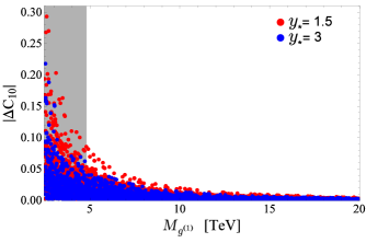
Figure 1: (color online) The $\text{RS}_{c}$ contribution to $|\Delta C_{10}|$ as a function of the KK gluon mass $M_{g^{(1)}}$ for two different values of $y_{\star}$. The gray region is excluded by the analysis of electroweak precision measurements.

The red and blue scatter points represent the cases of $y_{\star}=1.5$ and $3$, respectively. The gray region is excluded by the analysis of EW precision observables. It is clear that the smaller values of $M_{g^{(1)}}$ give larger deviations. Moreover, for a fixed value of $M_{g^{(1)}}$ a range of predictions for possible deviations are present for both cases of $y_{\star}$ such that the maximum allowed deviation for $|\Delta C_{10}|$ in the case of $y_{\star}=1.5$ are generally greater than the case of $y_{\star}=3$. This is due to the fact that in the case of $y_{\star}=3$, the SM fermions are more elementary as their profiles are localized towards the UV brane to a greater extent compared to the $y_{\star}=1.5$ case leading to more suppressed FCNC and subsequently smaller deviations in comparison to the case of $y_{\star}=1.5$.

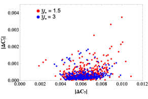
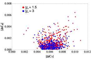
(a)	(b)
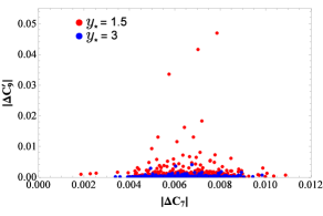
(c)	(d)
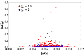
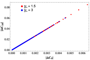
(e)	(f)

Figure 2: (color online) Correlations plots between the Wilson coefficients $|\Delta C^{(\prime)}_{7,\;9,\;10}|$ of the $\text{RS}_{c}$ model for a fixed value of $M_{g^{(1)}}=4.8$ TeV. The coefficients $\Delta C^{(\prime)}_{7}$ are calculated at the $\mu_{b}$ scale. The red and blue points correspond to $y_{\star}=1.5$ and $3$, respectively.

Observing the fact that the deviations for all $|\Delta C_{i}^{(\prime)}|$ for $M_{g^{(1)}}>10$ TeV are so small, as clear from Fig. 1 in the case of $|\Delta C_{10}|$, that the observables will almost remain unaffected, we limit the range for $M_{g^{(1)}}$ from $4.8$ TeV to $10$ TeV, where the lower value is implied by the EW precision constraints. As we are interested in the largest possible deviations of $|\Delta C_{i}^{(\prime)}|$, for a given allowed value of $M_{g^{(1)}}$, so we will take the $y_{\star}=1.5$ case and by considering five different values of $M_{g^{(1)}}\in[4.8,10]$, we obtain the maximum possible deviation of each Wilson coefficient. The resultant values will be used for evaluating the effects on the angular observables of interest for each considered value of $M_{g^{(1)}}$ in next section i.e., Sec. 5.2.

In Fig. 2, we show the correlation plots between $|\Delta C^{(\prime)}_{7,\;9,\;10}|$ obtained for the fixed value of $M_{g^{(1)}}=4.8$ TeV. The maximum possible deviations from the SM values in this case are

$$\left|\Delta C_{7}\right|_{max}=0.011,\text{ \ \ \ \ }\left|\Delta C_{9}\right|_{max}=0.0064,\text{ \ \ \ }\left|\Delta C_{10}\right|_{max}=0.085,$$

$$\left|\Delta C_{7}^{\prime}\right|_{max}=0.0037,\text{ \ \ \ \ }\left|\Delta C_{9}^{\prime}\right|_{max}=0.047,\text{ \ \ \ }\left|\Delta C_{10}^{\prime}\right|_{max}=0.621.$$

It is found that $|\Delta C_{9}|$ and $|\Delta C_{10}|$ are linearly correlated, as shown in Fig. 2(f), and same is true for each pair $|\Delta C_{i}^{(\prime)}|$ with $i=9,10$.

5.2 Angular observables

Table 1: Default values of the input parameters used in the calculations [87, 23].

$G_{F}=1.16638\times 10^{-5}$ GeV-2	$m_{t}^{\text{pole}}=174.2\pm 1.4$ GeV	$m_{\pi}=0.135$ GeV
$\alpha_{s}(m_{Z})=0.1182\pm 0.0012$	$m_{b}^{\text{pole}}=4.78\pm 0.06$ GeV	$m_{K}=0.494$ GeV
$\alpha(\mu_{b})=1/133.28$	$m_{c}^{\text{pole}}=1.67\pm 0.07$ GeV	$m_{B}=5.279$ GeV
$m_{W}=80.385\pm 0.015$ GeV	$m_{b}=4.18_{-0.03}^{+0.04}$ GeV	$m_{\Lambda_{b}}=5.619$ GeV
$m_{Z}=91.1876\pm 0.0021$ GeV	$m_{c}=1.27\pm 0.03$ GeV	$\tau_{\Lambda_{b}}=(1.466\pm 0.010)$ ps
$|V_{tb}V_{ts}^{\ast}|=0.04152$	$m_{s}=0.096_{-0.004}^{+0.008}$ GeV	$m_{\Lambda}=1.116$ GeV
$\alpha_{\Lambda}=0.642\pm 0.013$	$\mu_{b}=4.2$ GeV

In this section we discuss the numerical results computed for different angular observables both in the SM and for the $\text{RS}_{c}$ model. The input parameters used in the calculations are included in Table 1. The presented results include the uncertainty in the hadronic FFs, which are non-perturbative quantities. For this, we utilize the lattice QCD calculations [23], both in the low and high $q^{2}$ ranges, which till todate are considered as most accurate in the literature. To improve the accuracy, we have used the numerical values for the short-distance Wilson coefficients, with NNLL accuracy, at the low energy scale $\mu_{b}=4.2$ GeV, given in Table 2.

Table 2: The SM Wilson coefficients up-to NNLL accuracy given at $\mu_{b}=4.2$ GeV scale.

$C_{1}=-0.294$	$C_{2}=1.017$	$C_{3}=-0.0059$	$C_{4}=-0.087$	$C_{5}=0.0004$
$C_{6}=0.0011$	$C_{7}=-0.324$	$C_{8}=-0.176$	$C_{9}=4.114$	$C_{10}=-4.193$

The numerical results for the angular observables in appropriate bins are shown in Tables 3 and 4, where a comparison is presented between the predictions obtained for five different values of $M_{g^{(1)}}$ in the $\text{RS}_{c}$ model (for $y_{\star}=1.5$ ) to that of the SM estimates and with the experimental measurements, where available. The whole spectrum of di-muon mass squared (s $\epsilon$ $\{s_{min}=4m^{2}_{\mu},s_{max}=(m^{2}_{\Lambda_{b}}-m^{2}_{\Lambda})\}$) has not been discussed as the region $s\;\in$ $[8,15]$ GeV² is expected to receive sizable corrections from charmonium loops that violate quark-hadron duality. Hence the regions $s\;\in$ $[0.1,8]$ GeV² and $s\;\in[15,20]$ GeV² have been considered in order to avoid the long distance effects of charmonium resonances arising when lepton pair momenta approaches the masses of $J/\psi$ family. It can be seen that the results in the $\text{RS}_{c}$ model for most of the observables show little deviation from the SM predictions. Maximum deviation from the SM results has been observed for $M_{g^{(1)}}=4.8$ TeV and the difference gradually decreases as one moves from $M_{g^{(1)}}=4.8$ TeV to $M_{g^{(1)}}=10$ TeV.

Table 3: Numerical results of the observables (low $s$ region) in the $\Lambda_{b}\rightarrow\Lambda(\rightarrow p\pi)\mu^{+}\mu^{-}$ decay, obtained for the SM and the $\text{RS}_{c}$ model with $y_{\star}=1.5$ case, in different bins of low $s$. Experimentally measured values are taken from [22].

	$\ \left\langle\frac{d\mathcal{B}}{ds}\times 10^{-7}\right\rangle$	$\ \ \ \ \ \ \left\langle F_{L}\right\rangle$	$\ \ \ \ \ \ \left\langle A_{FB}^{\ell}\right\rangle$	$\ \ \ \ \ \left\langle A_{FB}^{\Lambda}\right\rangle$	$\ \ \ \ \ \ \left\langle A_{FB}^{l\Lambda}\right\rangle$
$[0.1,2]\begin{tabular}[]{l}$\text{SM}$\\ $\text{RS}_{c}|_{M_{g^{(1)}}}=4.8$\\ $\text{RS}_{c}|_{M_{g^{(1)}}}=6.1$\\ $\text{RS}_{c}|_{M_{g^{(1)}}}=7.4$\\ $\text{RS}_{c}|_{M_{g^{(1)}}}=8.7$\\ $\text{RS}_{c}|_{M_{g^{(1)}}}=10$\\ $\text{LHCb}$\end{tabular}$	$\ 0.238_{-0.230}^{+0.230}$ $\ 0.219_{-0.217}^{+0.218}$ $\ 0.225_{-0.217}^{+0.219}$ $\ 0.229_{-0.222}^{+0.224}$ $\ 0.232_{-0.223}^{+0.224}$ $\ 0.233_{-0.225}^{+0.228}$ $\ 0.36_{-0.112}^{+0.122}$	$\ \ \ \ 0.535_{-0.078}^{+0.065}$ $\ \ \ \ 0.552_{-0.084}^{+0.069}$ $\ \ \ \ 0.545_{-0.082}^{+0.067}$ $\ \ \ \ 0.542_{-0.081}^{+0.067}$ $\ \ \ \ 0.540_{-0.080}^{+0.066}$ $\ \ \ \ 0.539_{-0.080}^{+0.066}$ $\ \ \ \ 0.56_{-0.566}^{+0.244}$	$\ \ \ \ 0.097_{-0.007}^{+0.006}$ $\ \ \ \ 0.093_{-0.006}^{+0.005}$ $\ \ \ \ 0.095_{-0.006}^{+0.005}$ $\ \ \ \ 0.095_{-0.007}^{+0.006}$ $\ \ \ \ 0.096_{-0.007}^{+0.006}$ $\ \ \ \ 0.096_{-0.007}^{+0.006}$ $\ \ \ \ 0.37_{-0.481}^{+0.371}$	$\ \ -0.310_{-0.008}^{+0.015}$ $\ \ -0.313_{-0.004}^{+0.013}$ $\ \ -0.313_{-0.006}^{+0.014}$ $\ \ -0.312_{-0.007}^{+0.015}$ $\ \ -0.312_{-0.007}^{+0.015}$ $\ \ -0.311_{-0.007}^{+0.015}$ $\ \ -0.12_{-0.318}^{+0.344}$	$\ \ -0.031_{-0.002}^{+0.003}$ $\ \ -0.030_{-0.002}^{+0.003}$ $\ \ -0.030_{-0.002}^{+0.003}$ $\ \ -0.030_{-0.002}^{+0.003}$ $\ \ -0.031_{-0.002}^{+0.003}$ $\ \ -0.031_{-0.002}^{+0.003}$ $\ \ \ \ \ \ \ \ -$
$[2,4]\begin{tabular}[]{l}$\text{SM}$\\ $\text{RS}_{c}|_{M_{g^{(1)}}}=4.8$\\ $\text{RS}_{c}|_{M_{g^{(1)}}}=6.1$\\ $\text{RS}_{c}|_{M_{g^{(1)}}}=7.4$\\ $\text{RS}_{c}|_{M_{g^{(1)}}}=8.7$\\ $\text{RS}_{c}|_{M_{g^{(1)}}}=10$\\ $\text{LHCb}$\end{tabular}$	$\ 0.180_{-0.123}^{+0.123}$ $\ 0.171_{-0.117}^{+0.118}$ $\ 0.173_{-0.117}^{+0.118}$ $\ 0.175_{-0.118}^{+0.119}$ $\ 0.176_{-0.119}^{+0.119}$ $\ 0.177_{-0.120}^{+0.120}$ $\ 0.11_{-0.091}^{+0.120}$	$\ \ \ \ 0.855_{-0.012}^{+0.008}$ $\ \ \ \ 0.860_{-0.006}^{+0.008}$ $\ \ \ \ 0.859_{-0.008}^{+0.008}$ $\ \ \ \ 0.858_{-0.009}^{+0.008}$ $\ \ \ \ 0.857_{-0.010}^{+0.008}$ $\ \ \ \ 0.857_{-0.011}^{+0.008}$ $\ \ \ \ \ \ \ -$	$\ \ \ \ 0.054_{-0.030}^{+0.037}$ $\ \ \ \ 0.040_{-0.026}^{+0.035}$ $\ \ \ \ 0.045_{-0.028}^{+0.036}$ $\ \ \ \ 0.048_{-0.028}^{+0.036}$ $\ \ \ \ 0.050_{-0.029}^{+0.036}$ $\ \ \ \ 0.051_{-0.030}^{+0.037}$ $\ \ \ \ \ \ -$	$\ \ -0.306_{-0.012}^{+0.022}$ $\ \ -0.311_{-0.005}^{+0.016}$ $\ \ -0.311_{-0.008}^{+0.018}$ $\ \ -0.310_{-0.009}^{+0.020}$ $\ \ -0.310_{-0.010}^{+0.020}$ $\ \ -0.309_{-0.010}^{+0.021}$ $\ \ \ \ \ \ \ \ -$	$\ \ -0.016_{-0.009}^{+0.008}$ $\ \ -0.013_{-0.010}^{+0.009}$ $\ \ -0.014_{-0.009}^{+0.008}$ $\ \ 0.015_{-0.009}^{+0.008}$ $\ \ -0.015_{-0.009}^{+0.008}$ $\ \ -0.016_{-0.009}^{+0.008}$ $\ \ \ \ \ \ \ \ -$
$[4,6]\begin{tabular}[]{l}$\text{SM}$\\ $\text{RS}_{c}|_{M_{g^{(1)}}}=4.8$\\ $\text{RS}_{c}|_{M_{g^{(1)}}}=6.1$\\ $\text{RS}_{c}|_{M_{g^{(1)}}}=7.4$\\ $\text{RS}_{c}|_{M_{g^{(1)}}}=8.7$\\ $\text{RS}_{c}|_{M_{g^{(1)}}}=10$\\ $\text{LHCb}$\end{tabular}$	$\ 0.232_{-0.110}^{+0.110}$ $\ 0.224_{-0.108}^{+0.108}$ $\ 0.227_{-0.108}^{+0.109}$ $\ 0.228_{-0.109}^{+0.109}$ $\ 0.229_{-0.109}^{+0.109}$ $\ 0.230_{-0.110}^{+0.110}$ $\ 0.02_{-0.010}^{+0.091}$	$\ \ \ \ 0.807_{-0.012}^{+0.018}$ $\ \ \ \ 0.806_{-0.016}^{+0.021}$ $\ \ \ \ 0.807_{-0.015}^{+0.019}$ $\ \ \ \ 0.807_{-0.014}^{+0.019}$ $\ \ \ \ 0.807_{-0.013}^{+0.019}$ $\ \ \ \ 0.807_{-0.013}^{+0.019}$ $\ \ \ \ \ \ \ \ -$	$\ \ -0.063_{-0.026}^{+0.038}$ $\ \ -0.078_{-0.021}^{+0.034}$ $\ \ -0.072_{-0.022}^{+0.036}$ $\ \ -0.069_{-0.024}^{+0.037}$ $\ \ -0.068_{-0.024}^{+0.037}$ $\ \ -0.067_{-0.025}^{+0.037}$ $\ \ \ \ \ \ \ \ -$	$\ \ -0.311_{-0.008}^{+0.014}$ $\ \ -0.314_{-0.002}^{+0.008}$ $\ \ -0.314_{-0.004}^{+0.010}$ $\ \ -0.314_{-0.005}^{+0.012}$ $\ \ -0.314_{-0.006}^{+0.012}$ $\ \ -0.313_{-0.006}^{+0.013}$ $\ \ \ \ \ \ \ \ -$	$\ \ \ 0.021_{-0.009}^{+0.007}$ $\ \ \ 0.024_{-0.009}^{+0.008}$ $\ \ \ 0.023_{-0.009}^{+0.007}$ $\ \ \ 0.023_{-0.009}^{+0.007}$ $\ \ \ 0.022_{-0.009}^{+0.007}$ $\ \ \ 0.022_{-0.009}^{+0.007}$ $\ \ \ \ \ \ \ \ -$
$[6,8]\begin{tabular}[]{l}$\text{SM}$\\ $\text{RS}_{c}|_{M_{g^{(1)}}}=4.8$\\ $\text{RS}_{c}|_{M_{g^{(1)}}}=6.1$\\ $\text{RS}_{c}|_{M_{g^{(1)}}}=7.4$\\ $\text{RS}_{c}|_{M_{g^{(1)}}}=8.7$\\ $\text{RS}_{c}|_{M_{g^{(1)}}}=10$\\ $\text{LHCb}$\end{tabular}$	$\ 0.312_{-0.094}^{+0.094}$ $\ 0.306_{-0.093}^{+0.094}$ $\ 0.307_{-0.093}^{+0.094}$ $\ 0.308_{-0.093}^{+0.094}$ $\ 0.309_{-0.094}^{+0.094}$ $\ 0.310_{-0.094}^{+0.094}$ $\ 0.25_{-0.111}^{+0.120}$	$\ \ \ \ 0.724_{-0.014}^{+0.025}$ $\ \ \ \ 0.720_{-0.016}^{+0.026}$ $\ \ \ \ 0.721_{-0.016}^{+0.026}$ $\ \ \ \ 0.722_{-0.015}^{+0.025}$ $\ \ \ \ 0.723_{-0.015}^{+0.025}$ $\ \ \ \ 0.723_{-0.014}^{+0.025}$ $\ \ \ \ \ \ \ \ -$	$\ \ -0.162_{-0.017}^{+0.025}$ $\ \ -0.174_{-0.013}^{+0.021}$ $\ \ -0.170_{-0.014}^{+0.022}$ $\ \ -0.168_{-0.015}^{+0.023}$ $\ \ -0.166_{-0.016}^{+0.024}$ $\ \ -0.165_{-0.016}^{+0.024}$ $\ \ \ \ \ \ \ \ -$	$\ \ -0.317_{-0.004}^{+0.007}$ $\ \ -0.314_{-0.001}^{+0.002}$ $\ \ -0.317_{-0.001}^{+0.004}$ $\ \ -0.317_{-0.002}^{+0.005}$ $\ \ -0.317_{-0.002}^{+0.006}$ $\ \ -0.317_{-0.003}^{+0.006}$ $\ \ \ \ \ \ \ \ -$	$\ \ \ 0.052_{-0.007}^{+0.005}$ $\ \ \ 0.054_{-0.007}^{+0.005}$ $\ \ \ 0.054_{-0.007}^{+0.005}$ $\ \ \ 0.054_{-0.007}^{+0.005}$ $\ \ \ 0.053_{-0.007}^{+0.005}$ $\ \ \ 0.053_{-0.007}^{+0.006}$ $\ \ \ \ \ \ \ \ -$
$[1.1,6]\begin{tabular}[]{l}$\text{SM}$\\ $\text{RS}_{c}|_{M_{g^{(1)}}}=4.8$\\ $\text{RS}_{c}|_{M_{g^{(1)}}}=6.1$\\ $\text{RS}_{c}|_{M_{g^{(1)}}}=7.4$\\ $\text{RS}_{c}|_{M_{g^{(1)}}}=8.7$\\ $\text{RS}_{c}|_{M_{g^{(1)}}}=10$\\ $\text{LHCb}$\end{tabular}$	$\ 0.199_{-0.120}^{+0.120}$ $\ 0.190_{-0.119}^{+0.120}$ $\ 0.193_{-0.119}^{+0.120}$ $\ 0.195_{-0.119}^{+0.120}$ $\ 0.196_{-0.119}^{+0.120}$ $\ 0.197_{-0.120}^{+0.120}$ $\ 0.09_{-0.051}^{+0.061}$	$\ \ \ \ \ 0.818_{-0.011}^{+0.011}$ $\ \ \ \ \ 0.824_{-0.007}^{+0.010}$ $\ \ \ \ \ 0.821_{-0.008}^{+0.010}$ $\ \ \ \ \ 0.820_{-0.010}^{+0.010}$ $\ \ \ \ \ 0.819_{-0.010}^{+0.010}$ $\ \ \ \ \ 0.819_{-0.011}^{+0.011}$ $\ \ \ \ \ \ \ \ -$	$\ \ \ \ \ 0.009_{-0.018}^{+0.027}$ $\ \ \ -0.005_{-0.014}^{+0.025}$ $\ \ \ \ \ 0.001_{-0.015}^{+0.026}$ $\ \ \ \ \ 0.003_{-0.016}^{+0.026}$ $\ \ \ \ \ 0.005_{-0.016}^{+0.026}$ $\ \ \ \ \ 0.006_{-0.017}^{+0.026}$ $\ \ \ \ \ \ \ \ -$	$\ \ -0.309_{-0.010}^{+0.018}$ $\ \ -0.312_{-0.004}^{+0.012}$ $\ \ -0.312_{-0.006}^{+0.014}$ $\ \ -0.312_{-0.007}^{+0.016}$ $\ \ -0.311_{-0.008}^{+0.016}$ $\ \ -0.311_{-0.008}^{+0.017}$ $\ \ \ \ \ \ \ \ \ -$	$\ \ -0.002_{-0.005}^{+0.004}$ $\ \ \ \ 0.001_{-0.006}^{+0.005}$ $\ \ \ \ 0.000_{-0.006}^{+0.005}$ $\ \ -0.001_{-0.005}^{+0.005}$ $\ \ -0.001_{-0.005}^{+0.005}$ $\ \ -0.001_{-0.005}^{+0.004}$ $\ \ \ \ \ \ \ -$

Next, we compare our results of observables in the SM and the $\text{RS}_{c}$ model with the measurements from the LHCb experiment [22]. For most of the observables, results in the $\text{RS}_{c}$ model are close to that obtained for the SM in all bins of $s$ and this can be seen in Tables 3 and 4. The branching ratio for the four body decay process $\Lambda_{b}\rightarrow\Lambda(\rightarrow p\pi)\mu^{+}\mu^{-}$ in the $\text{RS}_{c}$ model (for $M_{g^{(1)}}=4.8$ TeV) shows a slight deviation at low recoil and almost no deviation at large recoil. For the bin $[1.1,6]$, the branching ratio in the SM and the $\text{RS}_{c}$ are $0.199_{-0.12}^{+0.12}$ and $0.190_{-0.119}^{+0.120}$ respectively which are $1.8\sigma$ and $1.9\sigma$ away from the measured value $0.09_{-0.051}^{+0.061}$. The situation is quite similar for all other bins of large recoil where values of observables do not change much even for $M_{g^{(1)}}=4.8$ TeV. For low recoil bin $[15,20]$, the SM and the $\text{RS}_{c}$ model results $0.753_{-0.069}^{+0.069}$ and $0.807_{-0.069}^{+0.069}$ deviate from the measured value by $4.7\sigma$ and $4.1\sigma$. It is noted that the differential branching ratio in the $\text{RS}_{c}$ model is lower than the SM at large recoil and higher than the SM at low recoil.

Table 4: Numerical results of the observables (high $s$ region) in the $\Lambda_{b}\rightarrow\Lambda(\rightarrow p\pi)\mu^{+}\mu^{-}$ decay, obtained for the SM and the $\text{RS}_{c}$ model with $y_{\star}=1.5$ case, in different bins of high $s$. Experimentally measured values are taken from [22].

	$\ \left\langle\frac{d\beta}{ds}\times 10^{-7}\right\rangle$	$\ \ \ \ \ \ \left\langle F_{L}\right\rangle$	$\ \ \ \ \ \ \left\langle A_{FB}^{\ell}\right\rangle$	$\ \ \ \ \left\langle A_{FB}^{\Lambda}\right\rangle$	$\ \ \ \left\langle A_{FB}^{l\Lambda}\right\rangle$
$[15,16]\begin{tabular}[]{l}$\text{SM}$\\ $\text{RS}_{c}|_{M_{g^{(1)}}}=4.8$\\ $\text{RS}_{c}|_{M_{g^{(1)}}}=6.1$\\ $\text{RS}_{c}|_{M_{g^{(1)}}}=7.4$\\ $\text{RS}_{c}|_{M_{g^{(1)}}}=8.7$\\ $\text{RS}_{c}|_{M_{g^{(1)}}}=10$\\ $\text{LHCb}$\\ \end{tabular}$	$\ 0.798_{-0.073}^{+0.073}$ $\ 0.832_{-0.073}^{+0.073}$ $\ 0.816_{-0.073}^{+0.073}$ $\ 0.810_{-0.073}^{+0.073}$ $\ 0.806_{-0.074}^{+0.074}$ $\ 0.804_{-0.074}^{+0.074}$ $\ 1.12_{-0.187}^{+0.197}$	$\ \ \ \ \ 0.454_{-0.017}^{+0.032}$ $\ \ \ \ \ 0.447_{-0.017}^{+0.033}$ $\ \ \ \ \ 0.450_{-0.017}^{+0.033}$ $\ \ \ \ \ 0.451_{-0.017}^{+0.032}$ $\ \ \ \ \ 0.452_{-0.017}^{+0.032}$ $\ \ \ \ \ 0.452_{-0.017}^{+0.032}$ $\ \ \ \ \ 0.49_{-0.304}^{+0.304}$	$\ \ \ -0.382_{-0.008}^{+0.017}$ $\ \ \ -0.365_{-0.006}^{+0.014}$ $\ \ \ -0.372_{-0.007}^{+0.015}$ $\ \ \ -0.375_{-0.007}^{+0.015}$ $\ \ \ -0.377_{-0.007}^{+0.016}$ $\ \ \ -0.378_{-0.008}^{+0.016}$ $\ \ \ -0.10_{-0.163}^{+0.183}$	$\ \ -0.307_{-0.004}^{+0.002}$ $\ \ -0.287_{-0.005}^{+0.003}$ $\ \ -0.296_{-0.005}^{+0.003}$ $\ \ -0.300_{-0.004}^{+0.003}$ $\ \ -0.302_{-0.004}^{+0.003}$ $\ \ -0.304_{-0.004}^{+0.002}$ $\ \ -0.19_{-0.163}^{+0.143}$	$\ \ \ \ 0.131_{-0.008}^{+0.004}$ $\ \ \ \ 0.132_{-0.008}^{+0.004}$ $\ \ \ \ 0.132_{-0.008}^{+0.004}$ $\ \ \ \ 0.132_{-0.008}^{+0.004}$ $\ \ \ \ 0.132_{-0.008}^{+0.004}$ $\ \ \ \ 0.132_{-0.008}^{+0.004}$ $\ \ \ \ \ \ \ \ -$
$[16,18]\begin{tabular}[]{l}$\text{SM}$\\ $\text{RS}_{c}|_{M_{g^{(1)}}}=4.8$\\ $\text{RS}_{c}|_{M_{g^{(1)}}}=6.1$\\ $\text{RS}_{c}|_{M_{g^{(1)}}}=7.4$\\ $\text{RS}_{c}|_{M_{g^{(1)}}}=8.7$\\ $\text{RS}_{c}|_{M_{g^{(1)}}}=10$\\ $\text{LHCb}$\end{tabular}$	$\ 0.825_{-0.075}^{+0.075}$ $\ 0.877_{-0.075}^{+0.075}$ $\ 0.855_{-0.075}^{+0.075}$ $\ 0.844_{-0.075}^{+0.075}$ $\ 0.838_{-0.075}^{+0.075}$ $\ 0.835_{-0.075}^{+0.075}$ $\ 1.22_{-0.152}^{+0.143}$	$\ \ \ \ \ 0.418_{-0.017}^{+0.033}$ $\ \ \ \ \ 0.411_{-0.017}^{+0.033}$ $\ \ \ \ \ 0.414_{-0.017}^{+0.033}$ $\ \ \ \ \ 0.415_{-0.017}^{+0.033}$ $\ \ \ \ \ 0.416_{-0.017}^{+0.033}$ $\ \ \ \ \ 0.416_{-0.017}^{+0.033}$ $\ \ \ \ \ 0.68_{-0.216}^{+0.158}$	$\ \ \ -0.381_{-0.006}^{+0.013}$ $\ \ \ -0.356_{-0.004}^{+0.010}$ $\ \ \ -0.366_{-0.005}^{+0.011}$ $\ \ \ -0.371_{-0.005}^{+0.012}$ $\ \ \ -0.374_{-0.005}^{+0.012}$ $\ \ \ -0.376_{-0.006}^{+0.012}$ $\ \ \ -0.07_{-0.127}^{+0.136}$	$\ \ -0.289_{-0.006}^{+0.005}$ $\ \ -0.265_{-0.006}^{+0.005}$ $\ \ -0.276_{-0.006}^{+0.005}$ $\ \ -0.280_{-0.006}^{+0.005}$ $\ \ -0.283_{-0.006}^{+0.005}$ $\ \ -0.284_{-0.006}^{+0.005}$ $\ \ -0.44_{-0.058}^{+0.104}$	$\ \ \ \ 0.141_{-0.008}^{+0.004}$ $\ \ \ \ 0.140_{-0.009}^{+0.004}$ $\ \ \ \ 0.141_{-0.008}^{+0.004}$ $\ \ \ \ 0.141_{-0.008}^{+0.004}$ $\ \ \ \ 0.141_{-0.008}^{+0.004}$ $\ \ \ \ 0.141_{-0.008}^{+0.004}$ $\ \ \ \ \ \ \ \ -$
$[18,20]\begin{tabular}[]{l}$\text{SM}$\\ $\text{RS}_{c}|_{M_{g^{(1)}}}=4.8$\\ $\text{RS}_{c}|_{M_{g^{(1)}}}=6.1$\\ $\text{RS}_{c}|_{M_{g^{(1)}}}=7.4$\\ $\text{RS}_{c}|_{M_{g^{(1)}}}=8.7$\\ $\text{RS}_{c}|_{M_{g^{(1)}}}=10$\\ $\text{LHCb}$\end{tabular}$	$\ 0.658_{-0.066}^{+0.066}$ $\ 0.726_{-0.066}^{+0.066}$ $\ 0.698_{-0.066}^{+0.066}$ $\ 0.685_{-0.066}^{+0.066}$ $\ 0.677_{-0.066}^{+0.066}$ $\ 0.672_{-0.066}^{+0.066}$ $\ 1.24_{-0.149}^{+0.152}$	$\ \ \ \ \ 0.371_{-0.019}^{+0.034}$ $\ \ \ \ \ 0.367_{-0.020}^{+0.034}$ $\ \ \ \ \ 0.368_{-0.019}^{+0.034}$ $\ \ \ \ \ 0.369_{-0.019}^{+0.034}$ $\ \ \ \ \ 0.370_{-0.019}^{+0.034}$ $\ \ \ \ \ 0.370_{-0.019}^{+0.034}$ $\ \ \ \ \ 0.62_{-0.273}^{+0.243}$	$\ \ \ -0.317_{-0.010}^{+0.010}$ $\ \ \ -0.286_{-0.010}^{+0.010}$ $\ \ \ -0.297_{-0.010}^{+0.010}$ $\ \ \ -0.303_{-0.010}^{+0.010}$ $\ \ \ -0.307_{-0.010}^{+0.010}$ $\ \ \ -0.309_{-0.010}^{+0.010}$ $\ \ \ \ \ 0.01_{-0.146}^{+0.155}$	$\ \ -0.227_{-0.011}^{+0.011}$ $\ \ -0.201_{-0.010}^{+0.010}$ $\ \ -0.211_{-0.010}^{+0.010}$ $\ \ -0.216_{-0.011}^{+0.011}$ $\ \ -0.219_{-0.011}^{+0.011}$ $\ \ -0.221_{-0.011}^{+0.011}$ $\ \ -0.13_{-0.124}^{+0.095}$	$\ \ \ 0.153_{-0.009}^{+0.005}$ $\ \ \ 0.151_{-0.009}^{+0.005}$ $\ \ \ 0.152_{-0.009}^{+0.005}$ $\ \ \ 0.152_{-0.009}^{+0.005}$ $\ \ \ 0.153_{-0.009}^{+0.005}$ $\ \ \ 0.153_{-0.009}^{+0.005}$ $\ \ \ \ \ \ \ -\ \$
$[15,20]\begin{tabular}[]{l}$\text{SM}$\\ $\text{RS}_{c}|_{M_{g^{(1)}}}=4.8$\\ $\text{RS}_{c}|_{M_{g^{(1)}}}=6.1$\\ $\text{RS}_{c}|_{M_{g^{(1)}}}=7.4$\\ $\text{RS}_{c}|_{M_{g^{(1)}}}=8.7$\\ $\text{RS}_{c}|_{M_{g^{(1)}}}=10$\\ $\text{LHCb}$\end{tabular}$	$\ 0.753_{-0.069}^{+0.069}$ $\ 0.807_{-0.069}^{+0.069}$ $\ 0.785_{-0.069}^{+0.069}$ $\ 0.774_{-0.069}^{+0.069}$ $\ 0.767_{-0.069}^{+0.069}$ $\ 0.764_{-0.069}^{+0.069}$ $\ 1.20_{-0.099}^{+0.092}$	$\ \ \ \ \ 0.409_{-0.018}^{+0.033}$ $\ \ \ \ \ 0.403_{-0.019}^{+0.034}$ $\ \ \ \ \ 0.405_{-0.019}^{+0.034}$ $\ \ \ \ \ 0.406_{-0.019}^{+0.033}$ $\ \ \ \ \ 0.407_{-0.019}^{+0.033}$ $\ \ \ \ \ 0.407_{-0.019}^{+0.033}$ $\ \ \ \ \ 0.61_{-0.143}^{+0.114}$	$\ \ \ -0.358_{-0.007}^{+0.012}$ $\ \ \ -0.332_{-0.009}^{+0.008}$ $\ \ \ -0.343_{-0.008}^{+0.010}$ $\ \ \ -0.348_{-0.007}^{+0.010}$ $\ \ \ -0.351_{-0.007}^{+0.011}$ $\ \ \ -0.353_{-0.007}^{+0.011}$ $\ \ \ -0.05_{-0.095}^{+0.095}$	$\ \ -0.271_{-0.011}^{+0.011}$ $\ \ -0.247_{-0.011}^{+0.011}$ $\ \ -0.257_{-0.011}^{+0.011}$ $\ \ -0.262_{-0.011}^{+0.011}$ $\ \ -0.264_{-0.011}^{+0.011}$ $\ \ -0.266_{-0.011}^{+0.011}$ $\ \ -0.29_{-0.081}^{+0.076}$	$\ \ \ 0.143_{-0.008}^{+0.005}$ $\ \ \ 0.142_{-0.009}^{+0.005}$ $\ \ \ 0.143_{-0.009}^{+0.005}$ $\ \ \ 0.143_{-0.009}^{+0.005}$ $\ \ \ 0.143_{-0.009}^{+0.005}$ $\ \ \ 0.143_{-0.008}^{+0.005}$ $\ \ \ \ \ \ \ -\ \ \$

In case of $F_{L}$, maximum deviation has been observed for the first bin $[0.1,2]$ GeV² where predictions in the SM and the $\text{RS}_{c}$ model are $\left\langle F_{L}\right\rangle_{SM}=0.535^{+0.065}_{-0.078}$ and $\left\langle F_{L}\right\rangle_{\text{RS}_{c}}=0.552_{-0.084}^{+0.069}$, respectively which vary from the measured value $0.56_{-0.566}^{+0.244}$ by $0.1\sigma$ and $0.02\sigma$, respectively. For most of the bins, deviation of $F_{L}$ in the $\text{RS}_{c}$ model from the SM is negligible. For low recoil bin $[15,20]$ GeV², the values in both models $\left\langle F_{L}\right\rangle_{SM}=0.409^{+0.033}_{-0.018}$, $\left\langle F_{L}\right\rangle_{\text{RS}_{c}}=0.403_{-0.019}^{+0.034}$ deviate from the experimental result $0.61^{+0.114}_{-0.143}$ in the same bin by $1.6\sigma$. At lower values of $s$ upto $4$ GeV², the $\text{RS}_{c}$ model results deviate from the SM values to a greater extent, whereas almost similar values of the $\text{RS}_{c}$ model are obtained for the rest of the spectrum.

For $A^{\ell}_{FB}$, small deviation in the $\text{RS}_{c}$ model exists from the SM at low recoil. In the first bin $[0.1,2]$ GeV²our calculated results in both models differ from the measured value by $0.6\sigma$. For large $s$ bin $[15,20]$ GeV², the values in both models $\left\langle A^{\ell}_{FB}\right\rangle_{\text{S}M}=-0.358_{-0.007}^{+0.012}$ and $\left\langle A^{\ell}_{FB}\right\rangle_{\text{RS}_{c}}=-0.332_{-0.009}^{+0.008}$ are very close to each other and are $3.2\sigma$ and $3.0\sigma$ away from the measured value $-0.05_{-0.095}^{+0.095}$ in the same bin.

For $A^{\Lambda}_{FB}$ in the bin $[15,20]$ GeV² results of the SM and the $\text{RS}_{c}$ model are $\left\langle A^{\Lambda}_{FB}\right\rangle_{\text{S}M}=-0.271_{-0.011}^{+0.011}$ and $\left\langle A^{\Lambda}_{FB}\right\rangle_{\text{RS}_{c}}=-0.247_{-0.011}^{+0.011}$ and deviate from the measured value of LHCb $-0.29_{-0.081}^{+0.076}$ by $0.2\sigma$ and $0.5\sigma$. For $A^{\ell\Lambda}_{FB}$, no sizable deviation from the SM has been observed in any $s$ bin for the $\text{RS}_{c}$ model.

6 Conclusions

In the work presented here, we have studied the angular observables of the theoretically clean decay $\Lambda_{b}\rightarrow\Lambda(\to p\pi^{-})\mu^{+}\mu^{-}$ in the SM and the Randall-Sundrum model with custodial protection. After performing the scan of the parameter space of the model in the light of current constraints, we have worked out the largest possible deviations in the Wilson coefficients $|\Delta C_{7,9,10}^{(\prime)}|$ from the SM predictions for different allowed values of KK gluon mass $M_{g^{(1)}}$. The resultant deviations are small and do not allow for large effects in the angular observables. Although for maximum possible deviations in Wilson coefficients, for $M_{g^{(1)}}=4.8$ TeV, in the $\text{RS}_{c}$ model, some of the observables receive considerable change in particular bins such as $\frac{d\mathcal{B}}{ds}$ and $A^{\ell}_{FB}$ in low recoil bin $[15,20]$ GeV² and $F_{L}$ in the bin $[0.1,2]$ GeV² but these deviations are still small to explain the large gap between the theoretical and experimental data. Therefore, it is concluded that under the present bounds on the mass of first KK gluon state $M_{g^{(1)}}$, observables are largely unaffected by the NP arising due to custodially protected RS model. Hence, the current constraints on the parameters of $\text{RS}_{c}$ are too strict to explain the observed deviations in different observables of $\Lambda_{b}\rightarrow\Lambda(\to p\pi^{-})\mu^{+}\mu^{-}$ decay.

References

• [1] LHCb Collaboration, R. Aaij et al., Test of lepton universality using $B^{+}\rightarrow K^{+}\ell^{+}\ell^{-}$ decays, Phys. Rev. Lett. 113 (2014) 151601, [arXiv:1406.6482].
• [2] LHCb Collaboration, R. Aaij et al., Test of lepton universality with $B^{0}\rightarrow K^{*0}\ell^{+}\ell^{-}$ decays, JHEP 08 (2017) 055, [arXiv:1705.05802].
• [3] W. Altmannshofer, P. Stangl, and D. M. Straub, Interpreting Hints for Lepton Flavor Universality Violation, Phys. Rev. D96 (2017), no. 5 055008, [arXiv:1704.05435].
• [4] G. D’Amico, M. Nardecchia, P. Panci, F. Sannino, A. Strumia, R. Torre, and A. Urbano, Flavour anomalies after the $R_{K^{*}}$ measurement, JHEP 09 (2017) 010, [arXiv:1704.05438].
• [5] L.-S. Geng, B. Grinstein, S. Jäger, J. Martin Camalich, X.-L. Ren, and R.-X. Shi, Towards the discovery of new physics with lepton-universality ratios of $b\to s\ell\ell$ decays, Phys. Rev. D96 (2017), no. 9 093006, [arXiv:1704.05446].
• [6] G. Hiller and I. Nisandzic, $R_{K}$ and $R_{K^{\ast}}$ beyond the standard model, Phys. Rev. D96 (2017), no. 3 035003, [arXiv:1704.05444].
• [7] LHCb Collaboration, R. Aaij et al., Differential branching fractions and isospin asymmetries of $B\to K^{(*)}\mu^{+}\mu^{-}$ decays, JHEP 06 (2014) 133, [arXiv:1403.8044].
• [8] LHCb Collaboration, R. Aaij et al., Differential branching fraction and angular analysis of the decay $B_{s}^{0}\to\phi\mu^{+}\mu^{-}$, JHEP 07 (2013) 084, [arXiv:1305.2168].
• [9] LHCb Collaboration, R. Aaij et al., Angular analysis and differential branching fraction of the decay $B^{0}_{s}\to\phi\mu^{+}\mu^{-}$, JHEP 09 (2015) 179, [arXiv:1506.08777].
• [10] LHCb Collaboration, R. Aaij et al., Measurement of Form-Factor-Independent Observables in the Decay $B^{0}\to K^{*0}\mu^{+}\mu^{-}$, Phys. Rev. Lett. 111 (2013) 191801, [arXiv:1308.1707].
• [11] LHCb Collaboration, R. Aaij et al., Angular analysis of the $B^{0}\to K^{*0}\mu^{+}\mu^{-}$ decay using 3 fb-1 of integrated luminosity, JHEP 02 (2016) 104, [arXiv:1512.04442].
• [12] Belle Collaboration, S. Wehle et al., Lepton-Flavor-Dependent Angular Analysis of $B\to K^{\ast}\ell^{+}\ell^{-}$, Phys. Rev. Lett. 118 (2017), no. 11 111801, [arXiv:1612.05014].
• [13] M. Ciuchini, A. M. Coutinho, M. Fedele, E. Franco, A. Paul, L. Silvestrini, and M. Valli, On Flavourful Easter eggs for New Physics hunger and Lepton Flavour Universality violation, Eur. Phys. J. C77 (2017), no. 10 688, [arXiv:1704.05447].
• [14] T. Hurth, F. Mahmoudi, D. Martinez Santos, and S. Neshatpour, Lepton nonuniversality in exclusive $b{\rightarrow}s{\ell}{\ell}$ decays, Phys. Rev. D96 (2017), no. 9 095034, [arXiv:1705.06274].
• [15] C.-W. Chiang, X.-G. He, J. Tandean, and X.-B. Yuan, $R_{K^{(*)}}$ and related $b\to s\ell\bar{\ell}$ anomalies in minimal flavor violation framework with $Z^{\prime}$ boson, Phys. Rev. D96 (2017), no. 11 115022, [arXiv:1706.02696].
• [16] B. Capdevila, A. Crivellin, S. Descotes-Genon, J. Matias, and J. Virto, Patterns of New Physics in $b\to s\ell^{+}\ell^{-}$ transitions in the light of recent data, JHEP 01 (2018) 093, [arXiv:1704.05340].
• [17] M. Kohda, T. Modak, and A. Soffer, Identifying a $Z^{\prime}$ behind $b\to s\ell\ell$ anomalies at the LHC, Phys. Rev. D97 (2018), no. 11 115019, [arXiv:1803.07492].
• [18] A. Falkowski, S. F. King, E. Perdomo, and M. Pierre, Flavourful $Z^{\prime}$ portal for vector-like neutrino Dark Matter and $R_{K^{(*)}}$, JHEP 08 (2018) 061, [arXiv:1803.04430].
• [19] T. Mannel and S. Recksiegel, Flavor changing neutral current decays of heavy baryons: The Case $\Lambda_{b}\to\Lambda\gamma$, J. Phys. G24 (1998) 979–990, [hep-ph/9701399].
• [20] C.-H. Chen and C. Q. Geng, Baryonic rare decays of $\Lambda_{b}\to\Lambda l^{+}l^{-}$, Phys. Rev. D64 (2001) 074001, [hep-ph/0106193].
• [21] CDF Collaboration, T. Aaltonen et al., Observation of the Baryonic Flavor-Changing Neutral Current Decay $\Lambda_{b}\to\Lambda\mu^{+}\mu^{-}$, Phys. Rev. Lett. 107 (2011) 201802, [arXiv:1107.3753].
• [22] LHCb Collaboration, R. Aaij et al., Differential branching fraction and angular analysis of $\Lambda^{0}_{b}\rightarrow\Lambda\mu^{+}\mu^{-}$ decays, JHEP 06 (2015) 115, [arXiv:1503.07138].
• [23] W. Detmold and S. Meinel, $\Lambda_{b}\to\Lambda\ell^{+}\ell^{-}$ form factors, differential branching fraction, and angular observables from lattice QCD with relativistic $b$ quarks, Phys. Rev. D93 (2016), no. 7 074501, [arXiv:1602.01399].
• [24] H.-Y. Cheng and B. Tseng, 1/M corrections to baryonic form-factors in the quark model, Phys. Rev. D53 (1996) 1457, [hep-ph/9502391]. [Erratum: Phys. Rev.D55,1697(1997)].
• [25] L. Mott and W. Roberts, Rare dileptonic decays of $\Lambda_{b}$ in a quark model, Int. J. Mod. Phys. A27 (2012) 1250016, [arXiv:1108.6129].
• [26] X.-G. He, T. Li, X.-Q. Li, and Y.-M. Wang, PQCD calculation for $\Lambda_{b}\to\Lambda\gamma$ in the standard model, Phys. Rev. D74 (2006) 034026, [hep-ph/0606025].
• [27] T. Feldmann and M. W. Y. Yip, Form Factors for $\Lambda_{b}\to\Lambda$ Transitions in SCET, Phys. Rev. D85 (2012) 014035, [arXiv:1111.1844]. [Erratum: Phys. Rev.D86,079901(2012)].
• [28] Y.-M. Wang, Y. Li, and C.-D. Lü, Rare Decays of $\Lambda_{b}\to\Lambda+\gamma$ and $\Lambda_{b}\to\Lambda+l^{+}l^{-}$ in the Light-cone Sum Rules, Eur. Phys. J. C59 (2009) 861–882, [arXiv:0804.0648].
• [29] Y.-M. Wang, Y.-L. Shen, and C.-D. Lü, $\Lambda_{b}\to p,\Lambda$ transition form factors from QCD light-cone sum rules, Phys. Rev. D80 (2009) 074012, [arXiv:0907.4008].
• [30] Y.-M. Wang and Y.-L. Shen, Perturbative Corrections to $\Lambda_{b}\to\Lambda$ Form Factors from QCD Light-Cone Sum Rules, JHEP 02 (2016) 179, [arXiv:1511.09036].
• [31] T. M. Aliev, A. Ozpineci, and M. Savci, New physics effects in $\Lambda_{b}\to\Lambda\ell^{+}\ell^{-}$ decay with lepton polarizations, Phys. Rev. D65 (2002) 115002, [hep-ph/0203045].
• [32] T. M. Aliev, A. Ozpineci, and M. Savci, Model independent analysis of $\Lambda$ baryon polarizations in $\Lambda_{b}\to\Lambda\ell^{+}\ell^{-}$ decay, Phys. Rev. D67 (2003) 035007, [hep-ph/0211447].
• [33] T. M. Aliev, V. Bashiry, and M. Savci, Double-lepton polarization asymmetries in $\Lambda_{b}\to\Lambda\ell^{+}\ell^{-}$ decay, Eur. Phys. J. C38 (2004) 283–295, [hep-ph/0409275].
• [34] G. Turan, The exclusive $\Lambda_{b}\to\Lambda\ell^{+}\ell^{-}$ decay in the general two Higgs doublet model, J. Phys. G31 (2005) 525–537.
• [35] A. K. Giri and R. Mohanta, Study of FCNC mediated $Z$ boson effect in the semileptonic rare baryonic decays $\Lambda_{b}\to\Lambda\ell^{+}\ell^{-}$, Eur. Phys. J. C45 (2006) 151–158, [hep-ph/0510171].
• [36] T. M. Aliev and M. Savci, $\Lambda_{b}\to\Lambda\ell^{+}\ell^{-}$ decay in universal extra dimensions, Eur. Phys. J. C50 (2007) 91–99, [hep-ph/0606225].
• [37] V. Bashiry and K. Azizi, The Effects of fourth generation in single lepton polarization on $\Lambda_{b}\to\Lambda\ell^{+}\ell^{-}$ decay, JHEP 07 (2007) 064, [hep-ph/0702044].
• [38] M. J. Aslam, Y.-M. Wang, and C.-D. Lü, Exclusive semileptonic decays of $\Lambda_{b}\to\Lambda l^{+}l^{-}$ in supersymmetric theories, Phys. Rev. D78 (2008) 114032, [arXiv:0808.2113].
• [39] Y.-M. Wang, M. J. Aslam, and C.-D. Lü, Rare decays of $\Lambda_{b}\to\Lambda\gamma$ and $\Lambda_{b}\to\Lambda l^{+}l^{-}$ in universal extra dimension model, Eur. Phys. J. C59 (2009) 847–860, [arXiv:0810.0609].
• [40] T. M. Aliev, K. Azizi, and M. Savci, Analysis of the $\Lambda_{b}\rightarrow\Lambda\ell^{+}\ell^{-}$ decay in QCD, Phys. Rev. D81 (2010) 056006, [arXiv:1001.0227].
• [41] K. Azizi and N. Katirci, Investigation of the $\Lambda_{b}\rightarrow\Lambda\ell^{+}\ell^{-}$ transition in universal extra dimension using form factors from full QCD, JHEP 01 (2011) 087, [arXiv:1011.5647].
• [42] K. Azizi and N. Katirci, Analysis of $\Lambda_{b}\to\Lambda\ell^{+}\ell^{-}$ Transition in $SM4$ using Form Factors from Full QCD, Eur. Phys. J. A48 (2012) 73, [arXiv:1112.5242].
• [43] K. Azizi, S. Kartal, A. T. Olgun, and Z. Tavukoglu, Comparative analysis of the semileptonic $\Lambda_{b}\rightarrow\Lambda\ell^{+}\ell^{-}$ transition in SM and different SUSY scenarios using form factors from full QCD, JHEP 10 (2012) 118, [arXiv:1208.2203].
• [44] T. Gutsche, M. A. Ivanov, J. G. Korner, V. E. Lyubovitskij, and P. Santorelli, Rare baryon decays $\Lambda_{b}\to\Lambda{l^{+}l^{-}}(l=e,\mu,\tau)$ and $\Lambda_{b}\to\Lambda\gamma$ : differential and total rates, lepton- and hadron-side forward-backward asymmetries, Phys. Rev. D87 (2013) 074031, [arXiv:1301.3737].
• [45] K. Azizi, S. Kartal, A. T. Olgun, and Z. Tavukoglu, Analysis of the semileptonic $\Lambda_{b}\rightarrow\Lambda\ell^{+}\ell^{-}$ transition in the topcolor-assisted technicolor model, Phys. Rev. D88 (2013), no. 7 075007, [arXiv:1307.3101].
• [46] M. A. Paracha, I. Ahmed, and M. J. Aslam, Imprints of CP violation asymmetries in rare $\Lambda_{b}\to\Lambda\ell^{+}\ell^{-}$ decay in family non-universal $Z^{\prime}$ model, PTEP 2015 (2015), no. 3 033B04, [arXiv:1408.4318].
• [47] P. Böer, T. Feldmann, and D. van Dyk, Angular Analysis of the Decay $\Lambda_{b}\to\Lambda(\to N\pi)\ell^{+}\ell^{-}$, JHEP 01 (2015) 155, [arXiv:1410.2115].
• [48] S. Meinel and D. van Dyk, Using $\Lambda_{b}\to\Lambda\mu^{+}\mu^{-}$ data within a Bayesian analysis of $|\Delta B|=|\Delta S|=1$ decays, Phys. Rev. D94 (2016), no. 1 013007, [arXiv:1603.02974].
• [49] S.-W. Wang and Y.-D. Yang, Analysis of $\Lambda_{b}\rightarrow$ $\Lambda\mu^{+}\mu^{-}$ decay in scalar leptoquark model, Adv. High Energy Phys. 2016 (2016) 5796131, [arXiv:1608.03662].
• [50] K. Azizi, A. T. Olgun, and Z. Tavukoglu, Impact of scalar leptoquarks on heavy baryonic decays, Adv. High Energy Phys. 2017 (2017) 7435876, [arXiv:1609.09678].
• [51] Q.-Y. Hu, X.-Q. Li, and Y.-D. Yang, The ${\Lambda_{b}\rightarrow\Lambda(\rightarrow p\pi^{-})\mu^{+}\mu^{-}}$ decay in the aligned two-Higgs-doublet model, Eur. Phys. J. C77 (2017), no. 4 228, [arXiv:1701.04029].
• [52] R. N. Faustov and V. O. Galkin, Rare $\Lambda_{b}\to\Lambda l^{+}l^{-}$ and $\Lambda_{b}\to\Lambda\gamma$ decays in the relativistic quark model, Phys. Rev. D96 (2017), no. 5 053006, [arXiv:1705.07741].
• [53] R. F. Alnahdi, T. Barakat, and H. A. Alhendi, Rare $\Lambda_{b}\to\Lambda\ell^{+}\ell^{-}$ decay in the two-Higgs doublet model of type-III, PTEP 2017 (2017), no. 7 073B04, [arXiv:1706.07361].
• [54] S. Roy, R. Sain, and R. Sinha, Lepton mass effects and angular observables in $\Lambda_{b}\to\Lambda(\to p\pi)\ell^{+}\ell^{-}$, Phys. Rev. D96 (2017), no. 11 116005, [arXiv:1710.01335].
• [55] D. Das, Model independent New Physics analysis in $\Lambda_{b}\to\Lambda\mu^{+}\mu^{-}$ decay, Eur. Phys. J. C78 (2018), no. 3 230, [arXiv:1802.09404].
• [56] A. Nasrullah, M. Jamil Aslam, and S. Shafaq, Analysis of angular observables of $\Lambda_{b}\to\Lambda(\to p\pi)\mu^{+}\mu^{-}$ decay in the standard and $Z^{\prime}$ models, PTEP 2018 (2018), no. 4 043B08, [arXiv:1803.06885].
• [57] T. Blake and M. Kreps, Angular distribution of polarised $\Lambda_{b}$ baryons decaying to $\Lambda\ell^{+}\ell^{-}$, JHEP 11 (2017) 138, [arXiv:1710.00746].
• [58] L. Randall and R. Sundrum, A Large mass hierarchy from a small extra dimension, Phys. Rev. Lett. 83 (1999) 3370–3373, [hep-ph/9905221].
• [59] G. Burdman, Flavor violation in warped extra dimensions and CP asymmetries in $B$ decays, Phys. Lett. B590 (2004) 86–94, [hep-ph/0310144].
• [60] K. Agashe, G. Perez, and A. Soni, Flavor structure of warped extra dimension models, Phys. Rev. D71 (2005) 016002, [hep-ph/0408134].
• [61] G. Moreau and J. I. Silva-Marcos, Flavor physics of the RS model with KK masses reachable at LHC, JHEP 03 (2006) 090, [hep-ph/0602155].
• [62] S. Casagrande, F. Goertz, U. Haisch, M. Neubert, and T. Pfoh, Flavor Physics in the Randall-Sundrum Model: I. Theoretical Setup and Electroweak Precision Tests, JHEP 10 (2008) 094, [arXiv:0807.4937].
• [63] M. Blanke, A. J. Buras, B. Duling, S. Gori, and A. Weiler, $\Delta F=2$ Observables and Fine-Tuning in a Warped Extra Dimension with Custodial Protection, JHEP 03 (2009) 001, [arXiv:0809.1073].
• [64] M. Blanke, A. J. Buras, B. Duling, K. Gemmler, and S. Gori, Rare K and B Decays in a Warped Extra Dimension with Custodial Protection, JHEP 03 (2009) 108, [arXiv:0812.3803].
• [65] M. E. Albrecht, M. Blanke, A. J. Buras, B. Duling, and K. Gemmler, Electroweak and Flavour Structure of a Warped Extra Dimension with Custodial Protection, JHEP 09 (2009) 064, [arXiv:0903.2415].
• [66] M. Bauer, S. Casagrande, U. Haisch, and M. Neubert, Flavor Physics in the Randall-Sundrum Model: II. Tree-Level Weak-Interaction Processes, JHEP 09 (2010) 017, [arXiv:0912.1625].
• [67] M. Blanke, B. Shakya, P. Tanedo, and Y. Tsai, The Birds and the Bs in RS: The $b\to s\gamma$ penguin in a warped extra dimension, JHEP 08 (2012) 038, [arXiv:1203.6650].
• [68] P. Biancofiore, P. Colangelo, and F. De Fazio, Rare semileptonic $B\to K^{*}\ell^{+}\ell^{-}$ decays in RSc model, Phys. Rev. D89 (2014), no. 9 095018, [arXiv:1403.2944].
• [69] P. Biancofiore, P. Colangelo, F. De Fazio, and E. Scrimieri, Exclusive $b\to s\nu\bar{\nu}$ induced transitions in RSc model, Eur. Phys. J. C75 (2015) 134, [arXiv:1408.5614].
• [70] C.-D. Lü, F. Munir, and Q. Qin, $b\to ss{\bar{d}}$ decay in Randall-Sundrum models, Chin. Phys. C41 (2017), no. 5 053106, [arXiv:1607.07713].
• [71] G. D’Ambrosio and A. M. Iyer, Flavour issues in warped custodial models: $B$ anomalies and rare $K$ decays, Eur. Phys. J. C78 (2018), no. 6 448, [arXiv:1712.08122].
• [72] M. Blanke and A. Crivellin, $B$ Meson Anomalies in a Pati-Salam Model within the Randall-Sundrum Background, Phys. Rev. Lett. 121 (2018), no. 1 011801, [arXiv:1801.07256].
• [73] K. Azizi, A. T. Olgun, and Z. Tavukoğlu, Comparative analysis of the $\Lambda_{b}\rightarrow\Lambda\ell^{+}\ell^{-}$ decay in the SM, SUSY and RS model with custodial protection, Phys. Rev. D92 (2015), no. 11 115025, [arXiv:1508.03980].
• [74] K. Agashe, R. Contino, L. Da Rold, and A. Pomarol, A Custodial symmetry for $Zb\bar{b}$, Phys. Lett. B641 (2006) 62–66, [hep-ph/0605341].
• [75] M. Carena, E. Ponton, J. Santiago, and C. E. M. Wagner, Light Kaluza Klein States in Randall-Sundrum Models with Custodial SU(2), Nucl. Phys. B759 (2006) 202–227, [hep-ph/0607106].
• [76] R. Contino, L. Da Rold, and A. Pomarol, Light custodians in natural composite Higgs models, Phys. Rev. D75 (2007) 055014, [hep-ph/0612048].
• [77] G. Cacciapaglia, C. Csaki, G. Marandella, and J. Terning, A New custodian for a realistic Higgsless model, Phys. Rev. D75 (2007) 015003, [hep-ph/0607146].
• [78] R. Malm, M. Neubert, and C. Schmell, Higgs Couplings and Phenomenology in a Warped Extra Dimension, JHEP 02 (2015) 008, [arXiv:1408.4456].
• [79] T. Gherghetta and A. Pomarol, Bulk fields and supersymmetry in a slice of AdS, Nucl. Phys. B586 (2000) 141–162, [hep-ph/0003129].
• [80] D. Du, A. X. El-Khadra, S. Gottlieb, A. S. Kronfeld, J. Laiho, E. Lunghi, R. S. Van de Water, and R. Zhou, Phenomenology of semileptonic B-meson decays with form factors from lattice QCD, Phys. Rev. D93 (2016), no. 3 034005, [arXiv:1510.02349].
• [81] M. Beneke, T. Feldmann, and D. Seidel, Systematic approach to exclusive $B\to Vl^{+}l^{-}$, $V\gamma$ decays, Nucl. Phys. B612 (2001) 25–58, [hep-ph/0106067].
• [82] H. H. Asatryan, H. M. Asatrian, C. Greub, and M. Walker, Calculation of two loop virtual corrections to $b\to sl^{+}l^{-}$ in the standard model, Phys. Rev. D65 (2002) 074004, [hep-ph/0109140].
• [83] C. Greub, V. Pilipp, and C. Schupbach, Analytic calculation of two-loop QCD corrections to $b\to sl^{+}l^{-}$ in the high $q^{2}$ region, JHEP 12 (2008) 040, [arXiv:0810.4077].
• [84] ATLAS Collaboration, G. Aad et al., A search for $t\overline{t}$ resonances using lepton-plus-jets events in proton-proton collisions at $\sqrt{s}=8$ TeV with the ATLAS detector, JHEP 08 (2015) 148, [arXiv:1505.07018].
• [85] CMS Collaboration, A. M. Sirunyan et al., Search for $t\overline{t}$ resonances in highly boosted lepton+jets and fully hadronic final states in proton-proton collisions at $\sqrt{s}=13$ TeV, JHEP 07 (2017) 001, [arXiv:1704.03366].
• [86] R. Malm, M. Neubert, K. Novotny, and C. Schmell, 5D Perspective on Higgs Production at the Boundary of a Warped Extra Dimension, JHEP 01 (2014) 173, [arXiv:1303.5702].
• [87] Particle Data Group Collaboration, C. Patrignani et al., Review of Particle Physics, Chin. Phys. C40 (2016), no. 10 100001.