Abstract

We establish the well-posedness of the transient van Roosbroeck system in three space dimensions under realistic assumptions on the data: non-smooth domains, discontinuous coefficient functions and mixed boundary conditions. Moreover, within this analysis, recombination terms may be concentrated on surfaces and interfaces and may not only depend on charge-carrier densities, but also on the electric field and currents. In particular, this includes Avalanche recombination. The proofs are based on recent abstract results on maximal parabolic and optimal elliptic regularity of divergence-form operators.

Key words and phrases: van Roosbroeck’s system, semiconductor device, Avalanche recombination, surface recombination, nonlinear parabolic system, heterogeneous material, discontinuous coefficients and data, mixed boundary conditions

2010 Mathematics Subject Classification. 35K57 (primary), 35K55, 78A35, 35R05, 35K45

Acknowledgements. The authors would like to thank Herbert Gajewski, Annegret Glitzky, Thomas Koprucki, Matthias Liero, Hagen Neidhardt and Marita Thomas for stimulating discussions and an ongoing exchange of ideas on this topic. K.D. was partially supported by the European Research Council via “ERC-2010-AdG no. 267802 (Analysis of Multiscale Systems Driven by Functionals)” and by the DFG International Research Training Group IRTG 1529.

1 Introduction

In 1950, van Roosbroeck [67] established a system of partial differential equations describing the dynamics of electron and hole densities in a semiconductor device due to drift and diffusion within a self-consistent electrical field. In 1964, Gummel [35] published the first report on the numerical solution of these drift–diffusion equations for an operating semiconductor device. In the mathematical literature, there are now a number of related models and results. For excellent overviews, see [46] or [54] and references therein. Very active recent areas of research are, for example, the modelling and analysis of hydrodynamic models, active interfaces, e.g. in solar cells, and organic semiconductors, [25, 26, 27, 33, 34, 45, 72]. In real device simulation, drift-diffusion formulations and adaptive codes based on van Roosbroeck’s system represent the state of the art, [15, 22, 66]. Regarding the numerics and analysis of these systems, we highlight three main difficulties:

• The devices exhibit non-smoothness, referring to non-smooth boundary regularity of their domains, inhomogeneous, mixed boundary conditions due to external contacts, and discountinuous material coefficients due to their heterogeneous, mostly layered, structure.

• The dynamics include nonlinearities of high order, both in the expressions for the currents and for recombination, depending, for example, on the electric field itself rather than its potential. A highly relevant prototype is Avalanche recombination.

• Some processes concentrate on or are active on lower-dimensional substructures only, like surfacial or interfacial recombination due to material structure or impurities.

The aim of this paper is to establish a functional analytic setting for van Roosbroeck’s system that allows us to simultaneously handle these aspects. It is tayolered exactly to the combination of a lack of regularity due to non-smoothness, and the need for regularity due to nonlinearity (we refer to a more detailed discussion in Section 4). In particular, even though interfacial recombination in general prevents the existence of strong solutions, we can show well-posedness in a suitable norm and Hölder regularity of solutions, cf. Theorem 5.1. These results provide a strong basis for further numerical analysis, cf. for example the discussion in 4.2, for the modeling of more complex devices and coupled effects, and for future optimization and optimal control of the system.
The first proof of global existence and uniqueness of weak solutions for van Roosbroeck’s system under realistic physical and geometrical conditions is due to Gajewski and Gröger [18, 19]. It was shown that the solution tends to thermodynamical equilibrium, if this is admitted by the boundary conditions. The key for proving these results is a Lyapunov functional. At least one serious drawback of these and related results is that only recombination terms are admissable which depend on the densities, and this mostly even under some additional structural conditions, see [17, 2.2.3], [20, Ch. 6], [23] and [71]. The only exception seems to be the paper of Seidman [68], where Avalanche generation – also called impact ionization, is included. However, his analytic framework requires (generically) smooth geometries and necessarily excludes mixed boundary conditions, cf. [68, Ch. 5], and interfacial recombination, which are essentially indispensable for real device modeling.
On the other hand, Avalanche generation is the determining operating priniciple of both Avalanche diodes and Avalanche transistors, [12, 39, 69], and it is of interest for modeling solar cells, see [51, 56]. In the case of Avalanche generation, no energy functional for van Roosbroeck’s system is known and, as is already observed in [68], methods based on maximum principles are not applicable. Thus, global existence cannot be expected (and may not be desirable) in such a general context, compare [16, 50], [55, p. 55].
Hence, our approach is different and rests on a reformulation of the system as the nonlocal quasilinear dynamics of the quasi Fermi levels, in an appropriate Banach space, cf. Section 4 and cf. [48] for a similar approach to the two-dimensional problem in an $L^{p}$-space without Avalanche recombination. We can then show well-posedness using maximal parabolic regularity of the linearized problem and the contraction mapping principle. Some special (mathematical) aspects of this approach are the following:

• It includes a detailed analysis of the nonlinear Poisson equation specific to the system. This also gives rise to efficient numerical schemes, compare [17] and the discussion in Subsection 4.2.

• A quite elaborate choice of the underlying Banach space, providing the spatial regularity of rates a.e. in time, cf. Section 5. In particular, spaces of types $L^{p}$ and $W^{-1,2}$ are excluded by non-smoothness, interfacial terms and nonlinearity, respectively, and spaces of type $W^{-1,p}$ are also not suitable. Our choice can be viewed as an adequate framework for the treatment of generalized second-order quasilinear parabolic problems with nonsmooth data when including semilinear terms that depend on (powers of) gradients of the unknowns.

• Many intricate properties of the non-smooth Poisson operators $-\mathrm{div}\,\mu\nabla\cdot$, entering in the equation for the electrostatic potential and the current fluxes, are essential to the analysis and were achieved only recently (see e.g. Proposition 5.4 and references):

  • They provide topological isomorphims between the spaces $W^{1,q}_{D}(\Omega)$ and $W^{-1,q}_{D}(\Omega)$ with $q$ larger than the space dimension $3$, cf. Assumption 3.5. An assumption like this was already introduced in [19] (compare [71, Introduction]) as an ad hoc assumption in order to show uniqueness in case of Fermi-Dirac statistics, but is now substantially covered by [8] in cases of mixed boundary conditions and heterogeneous, layered materials. Here, ‘layered’ can be interpreted in a fairly broad sense that may cover many specific devices.

  • They have maximal parabolic regularity, even when considered on interpolation spaces of $W^{-1,q}$ and $L^{q}$, cf. Proposition 5.4.

  • Even with varying coefficients due to the quasilinearity of the system, they have a (sufficiently regular) common domain of definition on these interpolation spaces, and the operator norm can be estimated suitably, cf. Lemma 5.7.

  • The domains of (suitable) fractional powers can be determined, due to the pioneering results of [4]. In particular, it can be shown that they may embed into $W^{1,q}$.

Even with some technicalities in the functional analytic framework, we want to present a main result that is straightforwardly applicable to real devices. Thus, we have taken care to motivate and discuss the mathematical assumptions, using known results, examples, relevant physical quantities and additional figures.
The outline of this paper is as follows: In the next section, we introduce van Roosbroeck’s model, including examples of expressions for bulk and surface recombination. In Section 3, we collect mathematical prerequisites. In particular, this includes assumptions and preliminary results associated to the non-smoothness of the setting and inhomogeneous data and to Avalanche recombination. In Section 4, we introduce and explain the functional analytic setting, analyse the nonlinear Poisson equation for the electrostatic potential given in terms of quasi Fermi levels, and deduce how the system can then be rewritten as a quasilinear abstract Cauchy problem. In Section 5, we prove the main result on well-posedness and discuss regularity of solutions.

2 The van Roosbroeck system

In this section we introduce the van Roosbroeck system for modeling the transport of charges in semiconductor devices. Therein, the negative and positive charge carriers, electrons and holes, move by diffusion and drift in a self-consistent electrical field and on their way, due to various mechanisms, they may recombine to charge-neutral electron-hole pairs or, vice versa, negative and positive charge carriers may be generated from charge-neutral electron-hole pairs.

The electronic state of the semiconductor device resulting from these phenomena is described by the triple $(u_{1},u_{2},\varphi)$ of unknowns that consists of

• the densities $u_{1}$ and $u_{2}$ of electrons and holes, and

• the electrostatic potential $\varphi$.

Moreover, further physical quantities associated with $(u_{1},u_{2},\varphi)$ are used to describe the state of the device:

• the chemical potentials $\chi_{1}$ and $\chi_{2}$,

• the quasi Fermi levels $\Phi_{1},\Phi_{2}$, and,

• the electron and hole currents $j_{1}$ and $j_{2}$.

Their precise relations are given in Section 2.1.

Throughout this work we assume that the semiconductor device occupies a bounded domain $\Omega\subset\mathbb{R}^{3}$. Its boundary $\partial\Omega$ with outer unit normal $\nu,$ consists of a Dirichlet part $D\subset\partial\Omega$ and of a Neumann, resp. Robin part $\Gamma:=\partial\Omega\backslash D$. In addition, two-dimensional interfaces $\Pi\subset\Omega$ are taken into account, where additional recombination mechanisms may take place, triggered e.g. by material impurities. The precise mathematical assumptions on the geometry of these objects are collected in Assumption 3.1. The evolution of the charge carriers is monitored during a finite time interval $J=]0,T[$ with $T\in]0,\infty[$.

The van Roosbroeck system (1), defined on $J\times\Omega$, then consists of the Poisson equation (1a) and the current continuity equations (1b):

$$\text{Poisson equation:}\hskip 85.35826pt-\mathrm{div}\left(\varepsilon\nabla\varphi\right) ={d}+u_{1}-u_{2} \text{in}\,\Omega,$$ (1a)

$$\varphi ={\varphi}_{D} \text{on }D,$$

$${\nu}\cdot{\left(\varepsilon\nabla\varphi\right)}+\varepsilon_{\Gamma}\varphi ={\varphi}_{\Gamma} \text{on }\Gamma,$$

and with $$k\in\{1,2\}, k=1 k=2$$ for electrons and for holes, the

$$\text{current-continuity equation:}\qquad\partial_{t}u_{k}-\text{div}j_{k} =r^{\Omega} \text{in }J\times(\Omega\setminus\Pi)$$ (1b)

$$\Phi_{k}(t) =\Phi_{k}^{D}(t) {D}$$ on ,

$${\nu}\cdot{j_{k}} ={r}^{\Gamma} \Gamma$$ on ,

$$[{\nu}\cdot{j_{k}}] ={r}^{\Pi} \Pi$$ on .

The evolution starts from initial conditions $$\Phi_{k}(0)=\Phi_{k,0}$$.

The parameters in the Poisson equation are the dielectric permittivity $\varepsilon:\Omega\to\mathbb{R}^{3\times 3}$ and, on the right-hand side, the (prescribed) doping profile $d$. The latter is allowed to be located also on a two-dimensional surface in $\overline{\Omega}$ (cf. [59] [11]), see our mathematical requirement on $d$ in Assumption 3.12 below. Moreover, in the corresponding boundary conditions, $\varepsilon_{\Gamma}:\Gamma\to[0,\infty)$ represents the capacity of the part of the corresponding device surface, ${\varphi}_{D}$ and ${\varphi}_{\Gamma}$ are the voltages applied at the contacts of the device, and may, therefore depend on time.
From now on we denote the pair $(\Phi_{1},\Phi_{2})$ of quasi Fermi levels by $\Phi$. Analogously, we always write $u$ for the pair of densities $(u_{1},u_{2})$.

The current-continuity equations feature the currents $j_{k}$ on their left-hand side and reaction or recombination terms $r^{\Omega},r^{\Gamma},r^{\Pi}$ on their right-hand side. Here, $r^{\Omega}$ acts in the bulk and, additionally, the Neumann conditions in (1b) balance the normal fluxes cross the exterior boundary $\Gamma$ with surface recombinations $r^{\Gamma}$ taking place on $\Gamma,$ resp. the jump of the normal fluxes $[{\nu}\cdot{j_{k}}]$ across $\Pi$ with surface recombinations ${r}^{\Pi}$ taking place on the surface $\Pi$. Details on $j_{k}$ and $r^{\Omega}$, $r^{\Gamma}$, $r^{\Pi}$ and in particular on their dependence of the quantities $u$,$\varphi$, and $\Phi$ are given in Sections 2.1 and 2.2.

2.1 Carrier densities and currents

An essential modeling ingredient of van Roosbroeck’s system is the relation of the densities of electrons and holes with their chemical potentials. We assume

$$u_{k}(t,x)=\mathcal{F}_{k}\left(\chi_{k}(t,x)\right)\,,\quad x\in\Omega,\qquad k=1,2,$$ (2)

where the functions $\mathcal{F}_{1}$ and $\mathcal{F}_{2}$ represent the statistical distribution of the electrons and holes in the energy band. In general, Fermi–Dirac statistics applies, i.e.

$$\mathcal{F}_{k}(s)=\frac{2}{\sqrt{\pi}}\int_{0}^{\infty}\frac{\sqrt{t}}{1+e^{(}t-s)}\,\mathrm{d}{t},\qquad s\in\mathbb{R},\qquad k=1,2.$$ (3)

Sometimes, Boltzmann statistics is a good approximation:

$$\mathcal{F}_{k}(s)=e^{s}.$$ (4)

As is common, we assume that the electron and hole current is driven by the gradient of the quasi Fermi level of electrons $\Phi_{1}$ and holes $\Phi_{2}$, respectively. More precisely, the currents are given by

$$j_{k}(t,x)=u_{k}(t,x)\mu_{k}(x)\,\nabla\Phi_{k}(t,x)\;,\quad x\in\Omega,\qquad k=1,2,$$ (5)

where the quasi Fermi levels $\Phi_{k}$ are related to the chemical potentials $\chi_{k}$ via

$$\chi_{k}=\Phi_{k}+(-1)^{k}\varphi,\quad k=1,2$$ (6)

Here, $\mu_{k}:\Omega\to\mathbb{R}^{3\times 3}$ are the mobility tensors for electrons and holes, respectively. We specify the mathematical prerequisites on the functions $\mathcal{F}_{k}$ in the following

Assumption 2.1.

The functions $\mathcal{F}_{k}\colon\mathbb{R}\to]0,\infty[$, $k=1,2$ are twice continuously differentiable with $\mathcal{F}_{k}(s)\to+\infty$ as $s\to+\infty$. Moreover, their derivatives $\mathcal{F}_{k}^{\prime}$ are bounded from above and below on bounded intervals by strictly positive constants.

This includes Boltzmann statistics (4), as well as Fermi–Dirac statistics (3), for the distribution functions.

2.2 Recombination terms

The recombination term $r^{\Omega}$ on the right-hand side of the current–continuity equations (1b) can be given by rather general functions of the electrostatic potential, of the currents, and of the vector of electron/hole densities. It describes the production of electrons and holes, respectively — production or destruction, depending on the sign. Our formulation of the reaction rates remains abstract, cf. Section 3, but in particular, it includes a variety of models for semiconductors. It covers non-radiative recombination like the Shockley–Read–Hall recombination due to phonon transition and Auger recombination (three particle transition) as well as Avalanche generation, see e.g. [65, 52, 17] and the references cited there.

2.2.1 Bulk recombination

A rather general model for many recombination terms, valid under any statistics, is

$$r^{\Omega}(u_{1},u_{2},\Phi_{1},\Phi_{2})=\hat{r}(u_{1},u_{2})\bigl{(}g-\exp(\Phi_{1}+\Phi_{2})\bigr{)},$$

cf. [6, Sect. 9.2]. In case of Boltzmann statistics, this includes the well-known Shockley–Read–Hall recombination (SRH) and the Auger recombination (AUG):
(SRH) Shockley–Read–Hall recombination :

$$r^{\Omega}_{SRH}=\frac{u_{1}u_{2}-n_{i}^{2}}{\tau_{2}(u_{1}+n_{1})+\tau_{1}(u_{2}+n_{2})},\qquad$$ (7)

where $n_{i}$ is the intrinsic carrier density, $n_{1}$, $n_{2}$ are reference densities, and $\tau_{1}$, $\tau_{2}$ are the lifetimes of electrons and holes, respectively. $n_{i}$, $n_{1}$, $n_{2}$, and $\tau_{1}$, $\tau_{2}$ are parameters of the semiconductor material.
(AUG) Auger recombination (three particle transitions):

$$r^{\Omega}_{Auger}=(u_{1}u_{2}-n_{i}^{2})(c_{1}^{Auger}u_{1}+c_{2}^{Auger}u_{2}),\qquad$$ (8)

where $c_{1}^{Auger}$ and $c_{2}^{Auger}$ are the Auger capture coefficients of electrons and holes, respectively, in the semiconductor material.
(AVA) An analytical expression for Avalanche generation (impact ionization), valid at least in the cases of Silicon or Germanium, is

$$r^{\Omega}_{Ava}(u,\varphi,\Phi)=c_{n}|j_{n}|\exp\Bigl{(}{\frac{-a_{n}}{|E\cdot\mathfrak{j}_{n}|}}\Bigr{)}+c_{p}|j_{p}|\exp\Bigl{(}{\frac{-a_{p}}{|E\cdot\mathfrak{j}_{p}|}}\Bigr{)},$$ (9)

where $E=\nabla\varphi$ is the electrical field and $\mathfrak{j}_{n,p}$ are the normalized currents $\frac{j_{n,p}}{|j_{n,p}|}$ of the corresponding type. The parameters $a,c_{n,p}$ are given, see [65, p. 111/112] and references; in particular Tables 4.2-3/4.2-4, and see also [55, Ch. p. 17, p. 54/55].

2.2.2 Surface recombination

Our model also allows for surface recombination terms $r^{\Gamma}$ along an exterior (Neumann/Robin) part of the boundary and $r^{\Pi}$ along interior, 2-dimensional surfaces $\Pi$, cf. [65, p. 110] and references given there, see also [23]. Of course, if $r^{\Gamma}\equiv 0$, then the semiconductor is isolated at $\Gamma$, i.e the current through $\Gamma$ is zero.
The functional analytic requirements on the reaction terms are specified in Subsection 3.4. A typical example of surface recombination is analogous to Shockley-Read-Hall, at gate contacts,

$$r^{\Gamma}_{Surf}(u)=\frac{u_{1}u_{2}-n_{i}^{2}}{v_{2}(u_{1}+n_{1})+v_{1}(u_{2}+n_{2})},$$

with additional parameters $v_{1},v_{2}$.

3 Mathematical prerequisites and assumptions

In this section, we introduce some mathematical terminology and state mathematical prerequisites for the analysis of the van Roosbroeck system (1).

In particular, we have the following requirements on the domain $\Omega$ occupied by the device. Figure 1 shows a typical example.

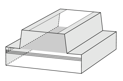
Figure 1: Scheme of a ridge waveguide quantum well laser (detail 3.2$\mu m\times 1.5\mu m\times 4\mu m$). The device domain has two material layers. The material interface (darkly shaded) and the Neumann boundary part (lightly shaded) meet at an edge. At the bottom and the top of the structure, contacts give rise to Dirichlet boundary conditions for the electrostatic potential. A triple quantum well structure is indicated where the light beam forms in the symmetry plane of the domain.

Assumption 3.1.

The device under consideration occupies a bounded domain $\Omega\subset\mathbb{R}^{3}$. The boundary $\partial\Omega$ is decomposed into a Dirichlet boundary part $D$ and its complement $\Gamma:=\partial\Omega\setminus D$. It holds that

• the Dirichlet boundary part $D$ is a $(d-1)$-set in the sense of Jonsson/Wallin, cf. [47, Ch. II]), and that

• every point $x$ in the closure of $\overline{\Gamma}$ admits a Lipschitzian boundary chart, cf. [57, Ch. 1.1.9]) or [30, Def. 1.2.1.2].

Moreover, $\Pi\subset\Omega$ is a Lipschitz surface (not necessarily connected) which forms a $(d-1)$-set, cf. [42, Ch. II/Ch. VIII.1], and $\sigma$ is the surface measure on $\Gamma\cup\Pi$, cf. [10, Ch. 3.3.4C] or [36, Ch. 3.1] (being identical with the restriction of the 2-dimensional Hausdorff measure to this set).

This defines the general geometric framework that is restricted implicitly later on by Assumption 3.5. We are convinced that this setting is sufficiently broad to cover (almost) all relevant semiconductor geometries – in particular, referring to the arrangement of $D$ and $\Gamma$. Please see also the more elaborate Remark 3.6 on this topic below.

3.1 Notation

For a Banach space $X$ we denote its norm by $\|{\cdot}\|_{X}$. $\mathbf{X}$ denotes the direct sum $X{\oplus}X$ of $X$ with itself. $\mathcal{L}(X;Y)$ is the space of linear, bounded operators from the Banach space $X$ into the Banach space $Y$. We abbreviate $\mathcal{L}(X):=\mathcal{L}(X;X)$. If $Z$ is a Banach space and $Z^{*}$ the space of (anti)linear forms on $Z$, then $\left\langle{\cdot}\,|\,{\cdot}\right\rangle_{Z}$ always denotes the (anti)dual pairing between $Z$ and $Z^{*}$.
The (standard) notation $[X,Y]_{\theta}$, $(X,Y)_{\theta,r}$, respectively, is used for the complex, respectively real interpolation spaces of $X$ and $Y$ with indices $\theta\in]0,1[$, $r\in[1,\infty]$. If $v$ is a function on an interval $J=]0,T[$ taking its values in a Banach space $X$, then $\dot{v}$ indicates its derivative in the sense of $X$-valued distributions, cf. [1, Ch. III.1.1].

3.2 Function spaces

We exemplarily define spaces of functions on the bounded domain $\Omega\subset\mathbb{R}^{3}$ and on its boundary. In the following, we (mostly) write $L^{2}$ instead of $L^{2}(\Omega)$ and use this convention for all spaces of functions, functionals or distributional objects on the bulk domain $\Omega$.
If $p\in[1,\infty]$, then $L^{p}$ is the usual real Lebesgue space on $\Omega$. $H^{\theta,q}$ denotes the space of real Bessel potentials (cf. [70, Ch. 4.2]), which coincides with the usual Sobolev space $W^{1,q}$ on $\Omega$ in case of $\theta=1$, cf. [70, Ch. 2.3.3]. $H^{\theta,q}_{{D}}$ denotes the closure of

$$C^{\infty}_{D}=\left\{\psi|_{\Omega}\,:\,\psi\in C^{\infty}_{0}(\mathbb{R}^{3}),\;\mathop{\rm supp}\psi\cap{D}=\emptyset\right\},$$

in $H^{\theta,q}$, which means that $H^{\theta,q}_{{D}}$ consists of all elements of $W^{1,q}$ with vanishing trace on ${D}$, – if the trace exists, compare [42, Thm. 3.7/Corollary 3.8]. $H^{-\theta,q}_{{D}}$ denotes the dual of $H^{\theta,q^{\prime}}_{D}$, where $\frac{1}{q}+\frac{1}{q^{\prime}}=1$. The requirements on $\Omega$ and on $D$ imply the usual interpolation properties within the $\{W^{1,q}_{D}\}_{q}$- and $\{W^{-1,q}_{D}\}_{q}$-scales, cf. [42].
If $Z$ is a Banach space and $A$ is a linear and closed operator in $Z$, then we denote its domain of definition by $dom_{Z}(A)$.

3.3 Weak elliptic operators in non-smooth settings

Before defining the elliptic operators relevant for (1), we introduce the following symmetry and ellipticity conditions:

Definition 3.2.

A bounded, measurable, elliptic coefficient function $\rho$ on $\Omega$ that takes its values in the set of symmetric $3\times 3$-matrices, is called an elliptic coefficient function. Bounded and elliptic means the existence of two constants ${\rho}_{\bullet}$ and ${\rho}^{\bullet}$ such that

$${\rho}_{\bullet}|\mathrm{y}|^{2}\leq{(\rho(x)\mathrm{y})}\cdot{\mathrm{y}}\leq{\rho}^{\bullet}|\mathrm{y}|^{2},\quad\text{for a.a. }x\in\Omega,\quad\text{for all }\mathrm{y}\in\mathbb{R}^{3}.$$

Assumption 3.3.

1. The dielectric permittivity $\varepsilon$ and the mobilities $\mu_{k}$, $k=1,2$ are elliptic coefficient functions.

2. We assume that either the boundary measure of the Dirichlet boundary part $D$ is positive or $\varepsilon_{\Gamma}$ is strictly positive on a subset of $\Gamma$ which has positive boundary measure. Physically spoken, the device has a Dirichlet contact or part of its surface has a positive capacity.

Considering the coefficient functions $\varepsilon$ and $\varepsilon_{\Gamma}$ from now on as fixed, we define the Robin Poisson operator $\widehat{P}:W^{1,2}\rightarrow W^{-1,2}_{D}$ by

$$\langle{\widehat{P}\psi}\,|\,{\vartheta}\rangle_{W^{1,2}_{D}}=\int_{{\Omega}}{(\varepsilon\nabla\psi)}\cdot{\nabla\vartheta}\,\mathrm{d}{x}+\int_{\Gamma}\varepsilon_{\Gamma}\psi\;\vartheta\,\mathrm{d}{{\sigma}},\;\psi\in{W}^{1,2},\;\vartheta\in{W}_{D}^{1,2}.$$ (10)

Correspondingly, $P$ denotes the restriction of $\widehat{P}$ to the domain ${W}_{D}^{1,2}$.
By a slight abuse of notation, $P$ may also denote the maximal restriction of $P$ to any range space which continuously embeds into ${W}_{D}^{-1,2}$.

Remark 3.4.

Assumption 3.3 assures that the Poisson operator is coercive, cf. [36] and [13], and, hence, $P:W^{1,2}_{D}\to W^{-1,2}_{D}$ is a topological isomorphism.

Let $\rho$ be an elliptic coefficient function on $\Omega$. Then we define the elliptic operator $A_{\rho}:W_{D}^{1,2}\rightarrow W^{-1,2}_{D}$ by

$$\langle{A_{\rho}\psi}\,|\,{\vartheta}\rangle_{W^{-1,2}_{D}}=\int_{{\Omega}}{(\rho\nabla\psi)}\cdot{\nabla\vartheta}\,\mathrm{d}{x},\quad\;\psi,\vartheta\in{W}_{D}^{1,2},$$ (11)

which may also denote its maximal restriction to a smaller range space. The operator $\widehat{A}_{\rho}$ is defined accordingly, acting on $W^{1,2}$. Of particular interest is the case $\rho=\eta\mu_{k}$, with $\eta$ a bounded, strictly positive scalar function.

For our analysis of van Roosbroeck’s system, the following assumption is crucial.

Assumption 3.5.

There is a common integrability exponent $q\in]3,4[$, such that the operators

$$P:W^{1,q}_{D}\to W^{-1,q}_{D}$$ (12)

and

$$A_{\mu_{k}}:W^{1,q}_{D}\to W^{-1,q}_{D},\;k=1,2,$$ (13)

are topological isomorphisms.

Remark 3.6.

1. Gajewski and Gröger have already observed in their pioneering paper [19] that a condition like this – in 1989 being an ad hoc assumption – would lead to a more satisfactory analysis of van Roosbroeck’s system, compare also the discussion in [71].

2. If (12) or (13) is a topological isomorphism for a $q>2$, then this property remains true for all $\tilde{q}\in[2,q[$ by Lax-Milgram and interpolation, cf. [42], so the set of such $q$s above $2$ always forms an interval. Thus, it is actually sufficient to assume that each of the operators in Assumption 3.5 is an isomorphism for some $q>3$. Moreover, if $A_{\rho}:W^{1,q}_{D}\to W^{-1,q}_{D}$ is a topological isomorphism, then this property is maintained for coefficient functions $\eta\rho$, if the scalar function $\eta$ is strictly positive and uniformly continuous on $\Omega$, cf. [8, Ch. 6].

3. Assumption 3.5 is fulfilled by very general classes of “layered” structures and additionally, if $D$ and its complement do not meet in a “too wild” manner, cf. [38] for the most relevant model settings. A global framework has recently been established in [8]. However, Assumption 3.5 indeed restricts the class of admissable coefficient functions $\varepsilon$ and $\mu_{k}$. For instance, it is typically not satisfied if three or more different materials meet at one edge.

4. Assumption 3.5 also includes interesting geometric constellations that are not covered in [8]. A relevant example are buried contacts, cf. Figure 2. The characteristic property of these constellations is that they touch themselves ‘from the other side’ – but only at the Dirichlet boundary part $D$. In particular, they need not be Lipschitz domains.

   

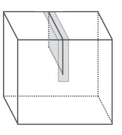
   Figure 2: Sketch of an idealized buried contact as an example of an admissible geometric setting. Dirichlet boundary conditions hold at the contact, i.e. on the shaded areas at the inner (buried) surface and close to its outer contact line.

5. Note that it is typically not restrictive to assume that all three differential operators provide topological isomorphisms, if one of them does, since this property mainly depends on the (possibly) discontinuous coefficient functions versus the geometry of $D$. This is determined by the material properties of the device on $\Omega$, i.e., the coefficient functions $\mu_{1},\mu_{2},\varepsilon$ will often exhibit similar discontinuities and degeneracies.

3.4 Assumptions on recombination terms in (1b)

For the recombination terms $r^{\Omega},$ $r^{\Pi},r^{\Gamma}$ in (1b), we require the following.

Assumption 3.7.

Let $q$ be as in Assumption 3.5. We assume that the reaction term in the bulk, $r^{\Omega}$, is a locally Lipschitzian mapping

$$r^{\Omega}:\mathbf{W}^{1,q}\times W^{1,q}\times{\mathbf{W}}^{1,q}\ni(u,\varphi,\Phi)\mapsto r^{\Omega}(u,\varphi,\Phi)\in L^{\frac{q}{2}}.$$

Assumption 3.8.

We assume that the reaction term on $\Gamma$, $r^{\Gamma}$, is a locally Lipschitzian mapping

$$r^{\Gamma}:\mathbf{W}^{1,q}\times W^{1,q}\times\mathbf{W}^{1,q}\ni(u,\varphi,\Phi)\mapsto r^{\Gamma}(u,\varphi,\Phi)\in L^{4}(\Gamma,\sigma).$$

The same assumption holds, mutatis mutandis, for $r^{\Pi}$.

In particular, the recombination terms introduced in (7) and (8) are included. It is nontrivial to see that the Avalanche generation term, depending on the electric field and the currents also satisfies Assumption 3.7. Since the generality of Assumption 3.7 causes considerable functional analytic effort in the analysis of the system, we give a detailed proof that Avalanche generation (9) is indeed included: It is straightforward to check that the mappings

$$L^{\infty}\times W^{1,q}\times W^{1,q}\ni(u_{k},\varphi,\Phi_{k})\mapsto\bigl{(}\nabla\varphi,j_{k}(u_{k},\Phi_{k})\bigr{)}\in\mathbf{L}^{q}(\Omega;\mathbb{R}^{3})$$

are boundedly Lipschitzian. If $\nabla\varphi$ and $j_{k}$ are orthogonal to each other, in order to give the expression in (9) a precise meaning, we introduce the function $\varkappa:\mathbb{R}^{3}\times\mathbb{R}^{3}\to[0,\infty[$ with

$$\varkappa(\mathfrak{e},\mathfrak{j})=\begin{cases}0,\quad\text{if}\quad\mathfrak{e}\cdot\mathfrak{j}=0,\\ |\mathfrak{j}|\exp(\frac{-a}{|\mathfrak{e}\cdot\frac{\mathfrak{j}}{|\mathfrak{j}|}|}),\quad\text{otherwise,}\end{cases}$$ (14)

for $a>0$. It then suffices to show the following result.

Lemma 3.9.

The mapping

$$L^{q}(\Omega;\mathbb{R}^{3})\times L^{q}(\Omega;\mathbb{R}^{3})\ni(\mathfrak{e},\mathfrak{j})\mapsto\varkappa\bigl{(}\mathfrak{e}(\cdot),\mathfrak{j}(\cdot)\bigr{)}$$

takes its values in the space $L^{q}(\Omega)$ and admits the Lipschitz estimate

$$\|\varkappa(\mathfrak{e}_{1},\mathfrak{j}_{1})-\varkappa(\mathfrak{e}_{2},\mathfrak{j}_{2})\|_{q/2}\leq(|\Omega|^{1/q}+2L_{a}\|\mathfrak{e}_{1}\|_{q})\|\mathfrak{j}_{1}-\mathfrak{j}_{2}\|_{q}+L_{a}\|\mathfrak{j}_{2}\|_{q}\|\mathfrak{e}_{1}-\mathfrak{e}_{2}\|_{q},$$ (15)

in $L^{q/2}(\Omega;\mathbb{R}^{3})$, where $\|\cdot\|_{q/2},\|\cdot\|_{q}$ are the norms in $L^{q/2}(\Omega;\mathbb{R}^{3})$, $L^{q}(\Omega;\mathbb{R}^{3})$, respectively, and where $L_{a}=\frac{4}{e^{2}a}<\frac{0.542}{a}$.

Proof.

For $\mathfrak{e},\mathfrak{j}\in\mathbb{R}^{3}$, we consider the function $\varkappa$ in (14) as composed of the functions $f_{a}\colon[0,+\infty[\ni t\mapsto e^{\frac{-a}{t}}$ and $\varpi\colon\mathbb{R}^{3}\times\mathbb{R}^{3}\ni(\mathfrak{e},\mathfrak{j})\mapsto|\mathfrak{e}\cdot\frac{\mathfrak{j}}{\|\mathfrak{j}\|}|$.Regarding $f_{a}$, note that it is analytic on $]0,+\infty[$, bounded by $1$, and has Lipschitz constant $L_{a}=\frac{4}{e^{2}a}$, and the last two properties extend into $0$. To show the Lipschitz estimate, consider $\mathfrak{e}_{1},\mathfrak{e}_{2},\mathfrak{j}_{1},\mathfrak{j}_{2}\in\mathbb{R}^{3}$. If $\mathfrak{j}_{1}=\mathfrak{j}_{2}=0$, then the estimate is trivial. Without loss of generality, let $\mathfrak{j}_{1}\neq 0$. Regarding $\varpi$, we estimate

$$|\varpi(\mathfrak{e}_{1},\mathfrak{j}_{1})-\varpi(\mathfrak{e}_{1},\mathfrak{j}_{2})|\leq\|\mathfrak{e}_{1}\|\frac{2}{\|\mathfrak{j}_{1}\|}\|\mathfrak{j}_{1}-\mathfrak{j}_{2}\|,$$

and

$$|\varpi(\mathfrak{e}_{1},\mathfrak{j}_{2})-\varpi(\mathfrak{e}_{2},\mathfrak{j}_{2})|\leq\|\mathfrak{e}_{1}-\mathfrak{e}_{2}\|.$$

Thus, we obtain

$$|\varkappa(\mathfrak{e}_{1},\mathfrak{j}_{1})-\varkappa(\mathfrak{e}_{2},\mathfrak{j}_{2})| \leq|\varkappa(\mathfrak{e}_{1},\mathfrak{j}_{1})-\varkappa(\mathfrak{e}_{1},\mathfrak{j}_{2})|+|\varkappa(\mathfrak{e}_{1},\mathfrak{j}_{2})-\varkappa(\mathfrak{e}_{2},\mathfrak{j}_{2})|$$

$$\leq\|\mathfrak{j}_{1}\||f_{a}(\varpi(\mathfrak{e}_{1},\mathfrak{j}_{1}))-f_{a}(\varpi(\mathfrak{e}_{1},\mathfrak{j}_{2}))|$$

$$\qquad+\|\mathfrak{j}_{1}-\mathfrak{j}_{2}\||f_{a}(\varpi(\mathfrak{e}_{1},\mathfrak{j}_{2}))|+L_{a}\|\mathfrak{e}_{1}-\mathfrak{e}_{2}\|$$

$$\leq(2L_{a}\|\mathfrak{e}_{1}\|+1)\|\mathfrak{j}_{1}-\mathfrak{j}_{2}\|+L_{a}\|\mathfrak{e}_{1}-\mathfrak{e}_{2}\|.$$

The estimate (15) now follows from Hölder’s inequality. ∎

3.5 Elliptic operators II: the domains of fractional powers

We choose an abstract formulation for the system that intricately solves the analytical problems arising from combining non-smoothness of material and geometry and nonlinearity of the dynamics. This gives rise to some technicalities in the proof. For example, on one hand, our techniques heavily rest on complex methods; this is in particular the instrument to provide exact descriptions for the domains of fractional powers of the elliptic operators involved. On the other hand, the system is intrisically a real one – of course, we are (only) interested in real solutions. In this subsection, we consider complex Banach spaces and complexifications of the elliptic operators $A_{\rho}$. In order to avoid further indices, the complex objects are denoted analogously to the real ones, only furnished by an underline.

Let $\rho$ be an elliptic coefficient function on $\Omega$. Then we define the elliptic operator $\underline{A}_{\rho}:\underline{W}_{D}^{1,2}\rightarrow\underline{W}^{-1,2}_{D}$ by

$$\langle{\underline{A}_{\rho}\psi_{1}}\,|\,{\psi_{2}}\rangle_{\underline{W}^{-1,2}_{D}}=\int_{{\Omega}}{(\rho\nabla\psi_{1})}\cdot{\nabla\overline{\psi}_{2}}\,\mathrm{d}{x},\quad\;\psi_{1},\psi_{2}\in\underline{W}_{D}^{1,2},$$

We show that the isomorphism property (13) transfers to the complex spaces.

Lemma 3.10.

If $\rho$ is a real, elliptic coefficient function, such that

$$A_{\rho}:W^{1,q}_{D}\to W^{-1,q}_{D}$$ (16)

is a topological isomorphism, then

$$\underline{A}_{\rho}:\underline{W}^{1,q}_{D}\to\underline{W}^{-1,q}_{D}$$ (17)

is a topological isomorphism.

Proof.

We define a *-operation in $\underline{W}^{-1,q}_{D}$ by setting $\langle f^{*}|\psi\rangle_{\underline{W}^{-1,q}_{D}}:=\overline{\langle f|\overline{\psi}\rangle_{\underline{W}^{-1,q}_{D}}},$ , for $\psi\in\underline{W}^{1,q^{\prime}}_{D}$. Evidently, one has $f=\frac{f+f^{*}}{2}+i\frac{f-f^{*}}{2i}$ and both $f_{1}:=\frac{f+f^{*}}{2}$ and $f_{2}:=\frac{f-f^{*}}{2i}$ attain real values for real functions $\psi\in W^{1,q^{\prime}}_{D}$ . Hence, $f_{1},f_{2}$ may be viewed as elements of the real space $W^{-1,q}_{D}$. Moreover, since $\underline{A}_{\rho}^{-1}$ transforms real elements $f=f^{*}\in W^{-1,q}_{D}$ into real functions, the isomorphism property (16) carries over to the one in (17). ∎

In case of smooth data (smooth domains, coefficients and absence of mixed boundary conditions) the determination of the domains of fractional powers is classical, cf. [64]. In our situation, this does not work, but the subsequent powerful results from [4] apply.

Proposition 3.11.

Assume $q\geq 2$ and let $\rho$ be an elliptic coefficient function on $\Omega$. Then

1. $(\underline{A}_{\rho}+1)^{\frac{1}{2}}$ provides a topological isomorphism of $\underline{L}^{q}$ and $\underline{W}^{-1,q}_{D}$,

2. the operator $\underline{A}_{\rho}+1$ is positive on both spaces, $\underline{L}^{q}$ and $\underline{W}^{-1,q}_{D}$, i.e. it satisfies resolvent estimates of the kind

   $$\|(\underline{A}_{\rho}+1+\lambda)^{-1}\|_{\mathcal{L}(\underline{L}^{q})}\leq\frac{1}{1+\lambda},\quad\|(\underline{A}_{\rho}+1+\lambda)^{-1}\|_{\mathcal{L}(\underline{W}^{-1,q}_{D})}\leq\frac{c}{1+\lambda},$$ (18)

   for all $\lambda\in[0,\infty[$ and some constant $c$, cf [70, Ch. 1.14]. In consequence, all fractional powers are well-defined, cf. [70, Ch. 1.15].

3. the operator $\underline{A}_{\rho}+1$ admits bounded purely imaginary powers on $\underline{W}^{-1,q}_{D}$, i.e. one has

   $$\sup_{\tau\in[0,1]}\|(\underline{A}_{\rho}+1)^{i\tau}\|_{\mathcal{L}(\underline{W}^{-1,q}_{D})}<\infty.$$

Proof.

i) is the main result of [4], see Thm. 5.1. Regarding ii), it is well-known that, under the above conditions, $\underline{A}_{\rho}$ generates a strongly continuous contraction semigroup on every $\underline{L}^{p}$, $p\in]1,\infty[$, cf. [60, Thm. 4.28]. Thus, the first resolvent estimate in (18) follows by the Hille-Yosida theorem, cf [63, Thm. X.47a]. The second estimate is deduced from the first by i). Finally, iii) is proved in [4, Ch. 11]. ∎

3.6 Inhomogeneous data

For setting up the Poisson and current–continuity equations in appropriate function spaces, we split the unknowns into two parts, where one part each represents the inhomogeneous Dirichlet boundary values ${\varphi}_{D}$ and $\Phi_{k}^{D}$, $k=1,2$.

Assumption 3.12.

The data $d,\varphi_{\Gamma},\varphi_{D}$ and $\Phi_{k}^{D}$ in (1) are such that

1. the doping $d$ is either contained in $W^{1,\infty}(J;L^{q/2})$ or it is independent of time and satisfies $d\in W^{-1,q}_{D}$, which would include dopings concentrated on surfaces, cf. [59] [11].

2. the Robin boundary value $\varphi_{\Gamma}$ satisfies $\varphi_{\Gamma}\in W^{1,\infty}(J;L^{4}(\Gamma,\sigma))$,

3. there are functions $\varphi^{D},\Phi^{d}_{k}\in W^{1,\infty}(J;L^{q/2})\cap L^{\infty}(J;W^{1,q})$ that also satisfy $\widehat{A}_{\mu_{k}}\Phi^{d}_{k},\widehat{P}\varphi^{D}\in L^{\infty}(J;L^{q/2})$ such that $\varphi^{D}(t)|_{D}=\varphi_{D}(t)$ and $\Phi^{d}_{k}(t)|_{D}=\Phi^{D}_{k}(t)$ in the sense of traces.

Remark 3.13.

Note that we do not suppose that the function $\varphi_{\Gamma}$ takes its values in $L^{\infty}(\Gamma,\sigma)$ with regularity assumptions for the dependence on time. If there were a continuity requirement on the mapping $\overline{J}\ni t\mapsto\varphi_{\Gamma}(t,\cdot)\in L^{\infty}(\Gamma,\sigma)$, this would exclude an indicator function of a subset of $\Gamma$ that moves in $\Gamma$ over time.

Remark 3.14.

The regularity Assumption 3.12 iii) is easily satisfied for smooth $\varphi_{D}$ and $\Phi^{D}$. In view of the fact that $D$ is a $(d-1)$-set of Jonsson/Wallin (cf. [47, Ch. II]), we refer to [42, Ch. V] for examples of suitable extension and trace operators. Note that additional time regularity of the data transfers to additional regularity of the solution, cf. Theorem 5.1 and Remark 5.3 below.

With Assumption 3.12, define

$$\varphi_{d}(t)=P^{-1}(d+\varphi_{\Gamma})(t)+(\mathrm{Id}-P^{-1}\widehat{P})\varphi^{D})(t)\in W^{-1,q}.$$

Then $\varphi_{d}$ solves

$$\left\{\begin{array}[]{rcll}-\mathrm{div}\,\varepsilon\nabla\varphi_{d}&=&d,&\text{in }\Omega,\\ \varphi_{d}&=&\varphi_{D},&\text{on }D,\\ \nu\cdot(\varepsilon\nabla\varphi_{d})+\varepsilon_{\Gamma}\varphi_{d}&=&\varphi_{\Gamma},&\text{on }\Gamma,\end{array}\right.$$

and the split

$$\varphi=\varphi_{d}+\tilde{\varphi}$$ (19)

gives a solution $\varphi$ of (1a) with

$$\tilde{\varphi}=P^{-1}(u_{1}-u_{2}).$$ (20)

For the quasi Fermi levels $\Phi_{k}$, in the following, we use the direct split

$$\Phi=\phi+\Phi^{d},$$ (21)

so that, in particular, $\phi(t)\in\mathbf{W}^{1,q}_{D}$ is equivalent to $\Phi(t)\in\mathbf{W}^{1,q}$ and $\Phi(t)|_{D}=\Phi^{D}(t)$.

4 Abstract formulation of (1)

In this section, we rewrite the van Roosbroeck system as a quasilinear abstract Cauchy problem for the homogeneous quasi Fermi levels $\phi_{1},\phi_{2}$,

$$\dot{\phi}(t)+\mathcal{A}(t,\phi(t))\phi(t)=\mathcal{R}(t,\phi(t))\in\mathbf{X},$$ (22)

with initial condition $\phi(0)=\Phi_{0}-\Phi^{d}(0)$. In the next subsection, we motivate and define the Banach space $\mathbf{X}$ – being a rather ‘unorthodox’ one – in which the problem is set. It becomes clear why the requirements due to the combination of non-smoothness and non-linearity of the system do not allow us to use an $L^{p}$- or an $W^{-1,2}_{D}$-space. We then prove the preliminary properties of the space $\mathbf{X}$ that justify its choice and are needed in the following.
To derive (22), we eliminate the electrostatic potential $\varphi$ from the continuity equations. Replacing the carrier densities $u_{1}$ and $u_{2}$ on the right hand side of Poisson’s equation by (2)/(6) – thereby taking into account (19) and (21) – one obtains a nonlinear Poisson equation for $\tilde{\varphi}$. In Subsection 4.2, we solve this equation in its dependence of prescribed quasi Fermi levels $\Phi\in\mathbf{W}^{1,q}$. This way of nesting the equations is also used in numerical schemes for the van Roosbroeck system. It is due to Gummel [35] and was the first reliable numerical technique to solve these equations for carriers in an operating semiconductor device structure.
Finally, in Subsection 4.3, we derive the abstract formulation of type (22).

4.1 Choice of the ambient space $\mathbf{X}$

We discuss structural and regularity properties of the unknowns $u,\varphi,\Phi$ of the transient semiconductor equations in (1) to motivate the choice of $\mathbf{X}$.

• In view of the jump condition on the surface $\Pi$ on the fluxes $j_{k}$ in (1b), it cannot be expected that $\mathrm{div}\,j_{k}$ is a function. This excludes spaces of type $L^{p}$, cf. Remark 5.3. In addition, with the choice of a space $\mathbf{X}$ that includes distributional objects, the inhomogeneous Neumann conditions $r^{\Gamma}$ in the current-continuity equations (1b) and the surface recombination term $r^{\Pi}$ can be included in the right-hand side of (22), cf. Lemma 4.4.

• For our analysis, we require an adequate parabolic theory for the divergence operators on $\mathbf{X}$. Due to the non-smooth geometry, the mixed boundary conditions and discontinous coefficient functions, this is nontrivial. The first crucial point is that the operators have to satisfy maximal parabolic regularity on $\mathbf{X}$, with a domain of definition that does not change, cf. Lemma 5.8.

• For the handling of ‘squares’ or other functions of gradients in the Avalanche and other recombination terms, the Banach space $X$ should be sufficienlty ‘small’ so that the parabolic time-trace space, cf. Theorem 5.1, embeds into $W^{1,q}$, cf. Corollary 5.9. This excludes spaces of type $W_{D}^{-1,r}$. With this strategy, at the same time, the space needs to be sufficiently large for the embedding $L^{q/2}\hookrightarrow X$ to hold, cf. Lemma 4.4.

• Finally, the dependence $\eta\mapsto A_{\eta\rho}$, cf. (11), should be well-behaved in the sense that it should be Lipschitz with respect to functions $\eta$ in the parabolic time-trace space, cf. Lemma 5.7.

With this discussion in mind, for $q>3$ the number from Assumption 3.5, we define

$$X:=[L^{q},W^{-1,q}_{D}]_{\frac{3}{q}}\quad\text{ and }\quad\mathbf{X}:=X\oplus X.$$

Moreover, we put $\mathcal{D}_{\mu}:=dom_{X}(A_{\mu_{1}})\oplus dom_{X}(A_{\mu_{2}})$, equipped with the graph norm.

Remark 4.1.

The complex interpolation functor applies to real spaces in the usual sense, following [1, Ch. 2.4.2]: the spaces are complexified, then interpolated and then the ‘real part’ is considered.

We show that $X$ and $\mathbf{X}$, respectively, together with the occurring operators, possess the properties claimed in the discussion.

Lemma 4.2.

Recall that $\underline{X}=[\underline{L}^{q},\underline{W}^{-1,q}_{D}]_{\frac{3}{q}}$. Assume that $\rho$ is an elliptic coefficient function, such that

$$A_{\rho}:W^{1,q}_{D}\to W^{-1,q}_{D}$$

is a topological isomorphism. Then

1. we have $dom_{\underline{W}^{-1,q}_{D}}\bigl{(}(\underline{A}_{\rho}+1)^{\frac{1}{2}(1-\frac{3}{q})})\bigr{)}=[\underline{L}^{q},\underline{W}^{-1,q}_{D}]_{\frac{3}{q}}$, and

2. the embedding

   $$\bigl{(}X,dom_{X}(A_{\rho})\bigr{)}_{\varsigma,\infty}\hookrightarrow W^{1,q},\quad\text{if}\quad\varsigma\in]\frac{1}{2}+\frac{3}{2q},1[.$$

Proof.

i) According to Proposition 3.11, $\underline{A}_{\rho}+1$ is a positive operator on $\underline{W}^{-1,q}_{D}$, possessing bounded purely imaginary powers. This gives, according to [70, Ch. 1.15.3],

$$dom_{\underline{W}^{-1,q}_{D}}\bigl{(}(\underline{A}_{\rho}+1)^{\frac{1}{2}(1-\frac{3}{q}}))\bigr{)}=[\underline{W}^{-1,q}_{D},dom_{\underline{W}^{-1,q}_{D}}\bigl{(}(\underline{A}_{\rho}+1)^{\frac{1}{2}}\bigr{)}]_{1-\frac{3}{q}}$$

$$=[\underline{W}^{-1,q}_{D},\underline{L}^{q}]_{1-\frac{3}{q}}=[\underline{L}^{q},\underline{W}^{-1,q}_{D}]_{\frac{3}{q}}=\underline{X}.$$

ii) From i), it immediately follows that $\bigl{(}\underline{A}_{\rho}+1)^{\frac{1}{2}(1+\frac{3}{q})}:\underline{W}^{1,q}_{D}\to[\underline{L}^{q},\underline{W}^{-1,q}_{D}]_{\frac{3}{q}}$ is a topological isomorphism; in other words $dom_{\underline{X}}\bigl{(}(\underline{A}_{\rho}+1)^{\frac{1}{2}(1+\frac{3}{q})}\bigr{)}=\underline{W}_{D}^{1,q}$. Since $\underline{A}_{\rho}$ is – by interpolation – also a positive operator on $\underline{X}$, for $\varsigma\in]\frac{1}{2}+\frac{3}{2q},1[$, we have

$$(\underline{X},dom_{X}(\underline{A}_{\rho}))_{\varsigma,\infty}\hookrightarrow(\underline{X},dom_{\underline{X}}(\underline{A}_{\rho}))_{\frac{1}{2}(1+\frac{3}{q}),1}\hookrightarrow dom_{\underline{X}}((\underline{A}_{\rho}+1)^{\frac{1}{2}(1+\frac{3}{q})})=\underline{W}^{1,q}_{D},$$

cf. [70, Thm. 1.3.3 e)] and [70, Thm. 1.15.2]). This proves the assertion in the complex case. But $X$ is a real subspace of $\underline{X}$ and $dom_{X}(A_{\rho})$ is a real subspace of $dom_{\underline{X}}(\underline{A}_{\rho})$. So the real interpolation space $\bigl{(}X,dom_{X}(A_{\rho})\bigr{)}_{\varsigma,\infty}$ must be embedded in the ‘real part’ $W^{1,q}_{D}$ of $\underline{W}^{1,q}_{D}$.
∎

Corollary 4.3.

Under Assumption 3.5, we obtain

$$\bigl{(}\mathbf{X},\mathcal{D}_{\mu}\bigr{)}_{\varsigma,\infty}\hookrightarrow\mathbf{W}_{D}^{1,q},\quad\text{if}\quad\varsigma\in]\frac{1}{2}+\frac{3}{2q},1[.$$

For convenience, we defined the recombination terms $r^{\Gamma}$ and $r^{\Pi}$ as $L^{4}(\Gamma,\sigma)$-valued and $L^{4}(\Pi,\sigma)$-valued, respectively, since one has an intuitive understanding of this condition. Since the whole system will be considered in the space $\mathbf{X}$, in the next result, we connect Assumption 3.8 with spaces of type $\mathbf{X}$.

Lemma 4.4.

Let $\Gamma$ and $\Pi$ be as in Assumption 3.1. Then

1. we have the embedding $L^{\frac{q}{2}}\hookrightarrow X$, and

2. there are continuous embeddings

   $$T^{*}_{\Gamma}\colon L^{4}(\Gamma,\sigma)\to X,\quad\text{and }\quad T^{*}_{\Pi}\colon L^{4}(\Pi,\sigma)\to X.$$

   given by the adjoints of the trace operators $T_{\Gamma},T_{\Pi}$.

Proof.

i) According to the duality formula for interpolation [70, Ch. 1.11.13],

$$[L^{q},W^{-1,q}_{D}]_{\theta}=[L^{q^{\prime}},W^{1,q^{\prime}}_{D}]^{*}_{\theta},$$

and taking into account Remark 4.1, the assertion is equivalent to $[\underline{L}^{q^{\prime}},\underline{W}^{1,q^{\prime}}_{D}]_{\frac{3}{q}}\hookrightarrow\underline{L}^{(\frac{q}{2})^{\prime}}$ . Exploiting the fact that the spaces $\underline{L}^{q^{\prime}}$ and $\underline{W}^{1,q^{\prime}}_{D}$ admit a common extension operator to $\underline{L}^{q^{\prime}}(\mathbb{R}^{3})$ and $\underline{W}^{1,q^{\prime}}(\mathbb{R}^{3})$, respectively, and the interpolation equality

$$[\underline{L}^{q^{\prime}}(\mathbb{R}^{3}),\underline{W}^{1,q^{\prime}}_{D}(\mathbb{R}^{3})]_{\frac{3}{q}}=\underline{H}^{\frac{3}{q},q^{\prime}}(\mathbb{R}^{3}),$$

one obtains, in combination with the embedding $\underline{H}^{\frac{3}{q},q^{\prime}}(\mathbb{R}^{3})\hookrightarrow\underline{L}^{(\frac{q}{2})^{\prime}}(\mathbb{R}^{3})$, the first assertion.
ii) We prove the dual statements, i.e. the existence of trace mappings

$$T_{\Gamma}\colon X^{*}=[L^{q^{\prime}},W^{1,q^{\prime}}_{D}]_{\frac{3}{q}}\to L^{\frac{4}{3}}(\Gamma,\sigma),\quad\text{and}\quad T_{\Pi}\colon X^{*}\to L^{\frac{4}{3}}(\Pi,\sigma),$$ (23)

thereby again taking into account Remark 4.1. In view of $q<4$, we have the inequalities $\frac{3}{q}>\frac{1}{q^{\prime}}=1-\frac{1}{q}$ and $q^{\prime}>\frac{4}{3}$. We establish the first trace mapping in (23). First, one may localize the setting. Then, thanks to the Lipschitz property of $\partial\Omega$ in a neighbourhood of $\overline{\Gamma}$, the bi-Lipschitzian boundary charts can be applied, observing that the quality of $[\underline{L}^{q^{\prime}},\underline{W}^{1,q^{\prime}}_{D}]_{\frac{3}{q}}\hookrightarrow[\underline{L}^{q^{\prime}},\underline{W}^{1,q^{\prime}}]_{\frac{3}{q}}$ is preserved under the corresponding transformation, so that the boundary part under consideration is ‘flat’. Hence, $[\underline{L}^{q^{\prime}},\underline{W}^{1,q^{\prime}}]_{\frac{3}{q}}=\underline{H}^{\frac{3}{q},q^{\prime}}$ can be applied locally, as in the half space case, [70, Thm. 2.10.1], in order to see that the trace belongs to $\underline{L}^{q^{\prime}}(\Gamma,\sigma)\hookrightarrow\underline{L}^{\frac{4}{3}}(\Gamma,\sigma)$.
We now establish the second trace mapping in (23). The starting point is the observation that the properties of $\Omega$, cf. Assumption 3.1, allow for a continuous extension operator $\mathfrak{E}:\underline{L}^{q^{\prime}}(\Omega)\to\underline{L}^{q^{\prime}}(\mathbb{R}^{3})$ the restriction of which to $\underline{W}_{D}^{1,q^{\prime}}(\Omega)$ provides a continuous operator into $\underline{W}^{1,q^{\prime}}(\mathbb{R}^{3})$, cf. [4, Lemma 3.2]. By interpolation, this gives a continuous extension operator

$$\hat{\mathfrak{E}}:\underline{X}^{*}=[\underline{L}^{q^{\prime}},\underline{W}^{1,q^{\prime}}_{D}]_{\frac{3}{q}}\to[\underline{L}^{q^{\prime}}(\mathbb{R}^{3}),\underline{W}^{1,q^{\prime}}(\mathbb{R}^{3})]_{\frac{3}{q}}=\underline{H}^{\frac{3}{q},q^{\prime}}(\mathbb{R}^{3}).$$

Taking $\tau\in]\frac{1}{q^{\prime}},\frac{3}{q}[\neq\emptyset$, we have the embedding $\underline{H}^{\frac{3}{q},q^{\prime}}(\mathbb{R}^{3})\hookrightarrow\underline{W}^{\tau,q^{\prime}}(\mathbb{R}^{3})$ into the corresponding Sobolev-Slobodetskii space, cf. [70, Ch. 4.6.1]. Now we consider $\overline{\Pi}$, the closure of $\Pi$, instead of $\Pi$, and exploit that $\overline{\Pi}$ is also a $2$-set, and $\overline{\Pi}\setminus\Pi$ is negligible with respect to the two-dimensional Hausdorff measure, cf. [47, Ch. VIII.1.1]). Then we use the trace mapping $\underline{W}^{\tau,q^{\prime}}(\mathbb{R}^{3})\hookrightarrow\underline{L}^{q^{\prime}}(\overline{\Pi},\sigma)\hookrightarrow\underline{L}^{\frac{4}{3}}(\overline{\Pi},\sigma)$, cf. [47, Ch. V.1.1]. Finally, the definition of the trace (cf. [47, Ch. I.2]) as the limit of averages (pointwise a.e. with respect to $\sigma$) tells us that the trace of any function $\psi\in H^{\frac{3}{q},q^{\prime}}$ on points of $\Pi$ is independent of the extension $\hat{\mathfrak{E}}\psi$, because $\Omega$ is open and $\Pi\subset\Omega$. ∎

4.2 The nonlinear Poisson equation

The aim of this subsection is to express the dependence of the homogeneous part of the electrostatic potential $\tilde{\varphi}$, cf. (19), in its dependence of the homogeneous quasi Fermi levels $\phi$. With $u_{k}(t)=\mathcal{F}_{k}\bigl{(}\phi(t)+\Phi^{d}_{k}(t)+(-1)^{k}(\tilde{\varphi}(t)+\varphi_{d}(t))\bigr{)}$ for some $\varphi_{d}(t),\Phi^{d}_{k}(t)\in L^{\infty}$ depending on the data, cf. Subsection 3.6, this means that we need to solve the nonlinear Poisson problem

$$P\tilde{\varphi}=\mathcal{F}_{1}(\omega_{1}-\tilde{\varphi})-\mathcal{F}_{2}(\omega_{2}+\tilde{\varphi})$$ (24)

and to quantify the dependence of the solution of given functions $\omega\in\mathbf{L}^{\infty}$.

With this analysis, we can then consider van Roosbroeck’s equations as a quasilinear nonlocal problem in the unknowns $\Phi$ only.

Theorem 4.5.

For every pair $\omega=(\omega_{1},\omega_{2})\in\mathbf{L}^{\infty}$ there is exactly one element $\tilde{\varphi}\in W^{1,q}_{D}$ that satisfies (24). We write $\tilde{\varphi}=\mathcal{S}(\omega)$. Then,

1. the mapping $\mathcal{S}:\mathbf{L}^{\infty}\to W^{1,q}_{D}$ is continuously differentiable,

2. the mapping $\mathcal{S}$, viewed between $\mathbf{L}^{\infty}$ and $L^{\infty}$, is globally Lipschitzian with Lipschitz constant not larger than $1$, and

3. $\mathcal{S}:\mathbf{L}^{\infty}\to W^{1,q}_{D}$ is boundedly Lipschitzian.

Proof.

We first apply the implicit function theorem. In particular, define

$$\mathcal{K}\colon\mathbf{L}^{\infty}\times W^{1,q}_{D}\to W^{-1,q}_{D}$$

by

$$\mathcal{K}(\omega,\tilde{\varphi})=P\tilde{\varphi}-\mathcal{F}_{1}(\omega_{1}-\tilde{\varphi})+\mathcal{F}_{2}(\omega_{2}+\tilde{\varphi}).$$

We show that $\mathcal{K}$ is continuously differentiable and that the partial derivatives with respect to $\tilde{\varphi}$ are topological isomorphisms between ${W}_{D}^{1,q}$ and ${W}_{D}^{-1,q}$. Then the level set $\mathcal{K}(\omega,\mathcal{S}(\omega))=0$ implicitly defines the solution operator

$$\mathcal{S}\colon\mathbf{L}^{\infty}\to W^{1,q}_{D}$$ (25)

of (24) and $\mathcal{S}$ is continuously differentiable. The partial derivatives of $\mathcal{K}$ are given by

$$\partial_{\tilde{\varphi}}\mathcal{K}(\omega,\tilde{\varphi}) = P+\sum_{k=1}^{2}\mathcal{F}^{\prime}_{k}(\omega_{k}+(-1)^{k}\tilde{\varphi})\in\mathcal{L}({W}_{D}^{1,q};{W}_{D}^{-1,q}),$$

$$\partial_{\omega_{k}}\mathcal{K}(\omega,\tilde{\varphi}) = (-1)^{k}\mathcal{F}^{\prime}_{k}(\omega_{k}+(-1)^{k}\tilde{\varphi})\in\mathcal{L}(L^{\infty};{W}_{D}^{-1,q}),$$

and they depend continuously on $\omega$ and $\tilde{\varphi}$. Note that here the expressions $\mathcal{F}^{\prime}_{k}(\omega_{k}+(-1)^{k}\tilde{\varphi})\in L^{\infty}$ are to be understood as multiplication operators.
Consider the equation

$$P\psi+\sum_{k=1}^{2}\mathcal{F}^{\prime}_{k}(\omega_{k}+(-1)^{k}\tilde{\varphi})\psi=f\in{W}_{D}^{-1,q}.$$ (26)

Since

$$\sum_{k=1}^{2}\mathcal{F}^{\prime}_{k}(\omega_{k}+(-1)^{k}\tilde{\varphi})$$

is a non-negative function in $L^{\infty}$, (26) has a unique solution $\psi\in{W}_{D}^{1,2}$ by the Lax-Milgram-Lemma. Moreover, $\sum_{k=1}^{2}\mathcal{F}^{\prime}_{k}(\omega_{k}+(-1)^{k}\tilde{\varphi})\psi$ is then contained in $L^{2}\hookrightarrow{W}_{D}^{-1,q}$ and $P\colon{W}_{D}^{1,q}\rightarrow{W}_{D}^{-1,q}$ is a topological isomorphism, so a rearrangement of terms in (26) gives $\psi\in{W}_{D}^{1,q}$. It follows that $\partial_{\tilde{\varphi}}\mathcal{K}(\omega,\tilde{\varphi})$ is an isomorphism of ${W}_{D}^{1,q}$ and ${W}_{D}^{-1,q}$. This proves i).
ii) Given $\omega,\kappa\in\mathbf{L}^{\infty}$, consider the solutions $\tilde{\varphi}=\mathcal{S}(\omega)\in W^{1,q}_{D}$, $\tilde{\psi}=\mathcal{S}(\kappa)\in W^{1,q}_{D}$ – each being even uniformly continuous. They satisfy

$$P(\tilde{\varphi}-\tilde{\psi})=\mathcal{F}_{1}(\omega_{1}-\tilde{\varphi})-\mathcal{F}_{2}(\omega_{2}+\tilde{\varphi})-\mathcal{F}_{1}(\kappa_{1}-\tilde{\psi})+\mathcal{F}_{2}(\kappa_{2}+\tilde{\psi})$$ (27)

in $W^{-1,q}_{D}\hookrightarrow W^{-1,2}_{D}$. Define

$$d=\max(\max(\|(\omega_{1}-\kappa_{1})^{+}\|_{\infty},\|(\kappa_{2}-\omega_{2})^{+}\|_{\infty}),\max(\|(\kappa_{1}-\omega_{1})^{+}\|_{\infty},\|(\omega_{2}-\kappa_{2})^{+}\|_{\infty})),$$

and note that $d\leq\|\omega-\kappa\|_{\mathbf{L}^{\infty}}$. Now let

$$h=\left\{\begin{array}[]{ll}\tilde{\varphi}-\tilde{\psi}-d,&\text{if }\tilde{\varphi}-\tilde{\psi}>d,\\ \tilde{\varphi}-\tilde{\psi}+d,&\text{if }\tilde{\varphi}-\tilde{\psi}<-d,\\ 0,&\text{otherwise}.\end{array}\right.$$

Taking into account the uniform continuity of $\tilde{\varphi},\tilde{\psi}$, it is not hard to see that $h$ is an admissable test function in $W^{1,2}_{D}\cap L^{\infty}$. Denote by $\Omega_{+}=\{x\in\Omega:h(x)>0\}$, $\Omega_{-}=\{x\in\Omega:h(x)<0\}$ the (open) subsets of $\Omega$ where $h$ is positive or negative, respectively. We apply (27) to $h$, cf. (10),

$$\begin{array}[]{rl}&\int_{\Omega}(\varepsilon\nabla h)\cdot\nabla h\,\mathrm{d}x+\int_{\Gamma}\varepsilon_{\Gamma}(\tilde{\varphi}-\tilde{\psi})h\,\mathrm{d}\sigma\\ =&\int_{\Omega_{+}}(\mathcal{F}_{1}(\omega_{1}-\tilde{\varphi})-\mathcal{F}_{1}(\kappa_{1}-\tilde{\psi}))h\,\mathrm{d}x-\int_{\Omega_{+}}(\mathcal{F}_{2}(\omega_{2}+\tilde{\varphi})-\mathcal{F}_{2}(\kappa_{2}+\tilde{\psi})h\,\mathrm{d}x\\ &+\int_{\Omega_{-}}(\mathcal{F}_{1}(\omega_{1}-\tilde{\varphi})-\mathcal{F}_{1}(\kappa_{1}-\tilde{\psi}))h\,\mathrm{d}x-\int_{\Omega_{-}}(\mathcal{F}_{2}(\omega_{2}+\tilde{\varphi})-\mathcal{F}_{2}(\kappa_{2}+\tilde{\psi})h\,\mathrm{d}x.\end{array}$$

Clearly, the first addend on the left-hand-side is non-negative. Secondly, the function $(\tilde{\varphi}-\tilde{\psi})h$ is non-negative on $\Omega$, so its trace on $\Gamma$ is also non-negative a.e. with respect to $\sigma$. On the other hand, by the definition of $d$ and $h$ and the monotonicity of $\mathcal{F}_{k}$, all four terms on the right-hand-side are non-positive. It follows that $h\equiv 0$ and thus

$$\|\tilde{\varphi}-\tilde{\psi}\|_{L^{\infty}}\leq d\leq\|\omega-\kappa\|_{\mathbf{L}^{\infty}},$$

which proves ii).
iii) is a direct consequence of re-investing ii) into (27), where

$$\|\tilde{\varphi}-\tilde{\psi}\|_{W^{1,q}_{D}}$$

$$\leq\|P^{-1}\|_{\mathcal{L}(L^{\infty};W^{1,q}_{D})}\|\mathcal{F}_{1}(\omega_{1}-\tilde{\varphi})-\mathcal{F}_{2}(\omega_{2}+\tilde{\varphi})-\mathcal{F}_{1}(\kappa_{1}-\tilde{\psi})+\mathcal{F}_{2}(\kappa_{2}+\tilde{\psi})\|_{\infty}$$

$$\leq C_{M}(\|\omega-\kappa\|_{\mathbf{L}^{\infty}}+\|\tilde{\varphi}-\tilde{\psi}\|_{\infty})$$

$$\leq 2C_{M}\|\omega-\kappa\|_{\mathbf{L}^{\infty}},$$

where the constant $C_{M}>0$ depends on the local Lipschitz constants of $\mathcal{F}_{k}$ with respect to bounded sets of parameters $\|\omega\|_{\mathbf{L}^{\infty}},\|\kappa\|_{\mathbf{L}^{\infty}}<M$. ∎

Remark 4.6.

We refer to [31] for a similar analysis of (24).

Theorem 4.5 is crucial for our result on well-posedness, but it also provides an adequate starting point for an highly effective numerical solution of the nonlinear Poisson equation. We discuss this point in some detail:
Given any $k_{1}\in\mathbb{R}$, e.g. $k_{1}=0$, with the choice of $k_{2}=\mathcal{F}_{2}^{-1}(\mathcal{F}_{1}(k_{1}))$, the pair $k=(k_{1},k_{2})$ is such that $\mathcal{S}(k)=0$. Set $K_{0}=\max(|k_{1}|,|k_{2}|)$ and note that $K_{0}=0$ is admissible if $\mathcal{F}_{1}=\mathcal{F}_{2}$, cf. the examples in Subsection 2.1. Then by Theorem 4.5 ii), for all $\omega=(\omega_{1},\omega_{2})$ with $\|\omega\|_{\infty}\leq M$, the set of solutions $\tilde{\varphi}=\mathcal{S}(\omega)$ is bounded via

$$\|\mathcal{S}(\omega)\|_{L^{\infty}}=\|\mathcal{S}(\omega)-\mathcal{S}(k)\|_{L^{\infty}}\leq\|\omega-k\|_{\mathbf{L}^{\infty}}\leq M+K_{0}.$$

We use this information in the following way: Let $K=M+K_{0}$, consider the function $\varpi$ with

$$\varpi(s)=\begin{cases}K,\quad\text{if}\quad s\geq K\\ s\quad\text{if}\quad s\in[-K,K]\\ -K\quad\text{if}\quad s\leq-K,\end{cases}$$

and denote the induced Nemytskii operator also by $\varpi$. Then $\tilde{\varphi}$ is a solution of (24) if and only if it satisfies the equation

$$P\tilde{\varphi}-\mathcal{F}_{1}(\omega_{1}-\varpi(\tilde{\varphi}))+\mathcal{F}_{2}(\omega_{2}+\varpi(\tilde{\varphi}))=0.$$ (28)

With this cut-off in the equation, it is straightforward to check that the associated operator

$$\mathcal{P}_{\omega}:W^{1,2}_{D}\ni\tilde{\psi}\mapsto P\tilde{\psi}-\mathcal{F}_{1}(\omega_{1}-\varpi(\tilde{\psi}))+\mathcal{F}_{2}(\omega_{2}+\varpi(\tilde{\psi}))\in W^{-1,2}_{D}$$

is well-defined, Lipschitzian and strongly monotonous with a monotonicity constant not smaller than the one for $P:W^{1,2}_{D}\to W^{-1,2}_{D}$ . The combination of monotonicity and Lipschitz continuity in a Hilbert space setting then provides a standard, highly efficient solution algorithm for (28), based on a contraction principle, see in particular [21, Ch. III.3.2].
Finally, a last point is interesting: due to the cut-off, these considerations do not depend on the asymptotics of the distribution functions $\mathcal{F}_{k}$ at $\infty$.

4.3 Quasilinear evolution of quasi-Fermi levels

In this subsection, we derive a quasilinear abstract Cauchy problem of type (22) that models the van-Roosbroeck system (1). It is the basis of our analysis and of a functional analytic setting in which both gradient recombination and interfacial jump conditions can be realized, cf. the discussion at the beginning of this section. In particular, the smoothing through the Poisson equation (1a) for the electrostatic potential can be fully exploited in this setting. We first give a pointwise reformulation of the bulk equations in (1) in terms of the evolution of the quasi Fermi levels $\Phi_{k}$ in (32) and then derive a suitable weak formulation in the space $\mathbf{X}$. With the definition (6) of the quasi Fermi levels we have

$$\dot{\Phi}_{k}=\frac{1}{\mathcal{F}_{k}^{\prime}(\chi_{k})}\dot{u}_{k}-(-1)^{k}\dot{\varphi}.$$ (29)

When recalling the split $\varphi=\tilde{\varphi}+\varphi_{d}$ from (19), and differentiating (20) (formally) with respect to time, we get

$$\dot{\varphi}=\dot{\varphi_{d}}+P^{-1}(\dot{u}_{1}-\dot{u}_{2}).$$ (30)

According to the defintion of the current densities (5), we get

$$\frac{1}{\mathcal{F}_{k}^{\prime}(\chi_{k})}\mathrm{div}\,j_{k}=\mathrm{div}(\frac{\mathcal{F}_{k}}{\mathcal{F}_{k}^{\prime}}(\chi_{k})\mu_{k}\nabla\Phi_{k})-\nabla(\frac{\mathcal{F}_{k}}{\mathcal{F}_{k}^{\prime}}(\chi_{k})-\chi_{k})\cdot\mu_{k}\nabla\Phi_{k}.$$ (31)

Combining (29), (30) and (31) with the bulk equations in (1b), we obtain the equations

$$\begin{array}[]{rcl}\left(\begin{array}[]{c}\dot{\Phi}_{1}\\ \dot{\Phi}_{2}\end{array}\right)\!\!\!&-&\!\!\!\left(\begin{array}[]{cc}1+P^{-1}\mathcal{F}_{1}^{\prime}(\chi_{1})&-P^{-1}\mathcal{F}_{2}^{\prime}(\chi_{2})\\ -P^{-1}\mathcal{F}_{1}^{\prime}(\chi_{1})&1+P^{-1}\mathcal{F}_{2}^{\prime}(\chi_{2})\end{array}\right)\left(\begin{array}[]{c}\mathrm{div}(\frac{\mathcal{F}_{1}}{\mathcal{F}_{1}^{\prime}}(\chi_{1})\mu_{1}\nabla\Phi_{1})\\ \mathrm{div}(\frac{\mathcal{F}_{2}}{\mathcal{F}_{2}^{\prime}}(\chi_{2})\mu_{2}\nabla\Phi_{2})\end{array}\right)\\ \!\!\!&=&\!\!\!-\left(\begin{array}[]{cc}1+P^{-1}\mathcal{F}_{1}^{\prime}(\chi_{1})&-P^{-1}\mathcal{F}_{2}^{\prime}(\chi_{2})\\ -P^{-1}\mathcal{F}_{1}^{\prime}(\chi_{1})&1+P^{-1}\mathcal{F}_{2}^{\prime}(\chi_{2})\end{array}\right)\left(\begin{array}[]{c}\nabla(\frac{\mathcal{F}_{1}}{\mathcal{F}_{1}^{\prime}}(\chi_{1})-\chi_{1})\cdot\mu_{1}\nabla\Phi_{1}\\ \nabla(\frac{\mathcal{F}_{2}}{\mathcal{F}_{2}^{\prime}}(\chi_{2})-\chi_{2})\cdot\mu_{2}\nabla\Phi_{2}\end{array}\right)\\ \!\!\!&&\!\!\!+\left(\begin{array}[]{c}\frac{1}{\mathcal{F}_{1}^{\prime}(\chi_{1})}\\ \frac{1}{\mathcal{F}_{2}^{\prime}(\chi_{2})}\end{array}\right)r^{\Omega}+\left(\begin{array}[]{c}+1\\ -1\end{array}\right)\dot{\varphi}_{d}.\end{array}$$ (32)

in $J\times\Omega$.
To incorporate the boundary and interface conditions in (1b), we use the split

$$\Phi_{k}=\Phi_{k}^{d}+\phi_{k},$$

cf. Subsection 3.6. We can now consider the densities $u$ in (1) as functions of $\phi$ via

$$u_{k}=\mathcal{F}_{k}(\chi_{k}),\;with\;\chi_{k}=\phi_{k}+\Phi_{k}^{d}+(-1)^{k}\varphi_{d}+(-1)^{k}\mathcal{S}(\phi+\Phi^{d}+\check{\varphi}^{d}),$$ (33)

where $\mathcal{S}$ taken from (25) is the solution operator of the nonlinear Poisson problem (24) and with the notation

$$\check{\varphi}^{d}=\left(\begin{array}[]{c}+1\\ -1\end{array}\right)\varphi_{d}.$$

In the following, considering $\varphi_{d}$ and $\Phi^{d}$ as fixed, for $\phi\in\mathbf{W}^{1,q}_{D}$, we thus define

$$\tilde{\mathcal{F}}_{k}(t,\phi)=\mathcal{F}_{k}(\chi_{k}(t))$$

with the right-hand-side as in (33) and, correspondingly, $\tilde{\mathcal{F}}_{k}^{\prime}(t,\phi)=\mathcal{F}_{k}^{\prime}(\chi_{k}(t))$, and

$$\eta_{k}(t,\phi)=\frac{\tilde{\mathcal{F}}_{k}(t,\phi_{k})}{\tilde{\mathcal{F}}_{k}^{\prime}(t,\phi_{k})}.$$

As an additional shorthand, we write

$$\left(\begin{array}[]{cc}1+P^{-1}\mathcal{F}_{1}^{\prime}(\chi_{1})&-P^{-1}\mathcal{F}_{2}^{\prime}(\chi_{2})\\ -P^{-1}\mathcal{F}_{1}^{\prime}(\chi_{1})&1+P^{-1}\mathcal{F}_{2}^{\prime}(\chi_{2})\end{array}\right)=\mathrm{Id}+P^{-1}[\tilde{\mathcal{F}}^{\prime}(t,\phi)],$$

for the matrix operators in (32).
We can now define the abstract evolution problem (1), in a functional analytic setting in which Neumann boundary and interfacial recombination terms appear on the right-hand-sides,

$$\dot{\phi}(t)+\mathcal{A}(t,\phi(t))\phi(t)=\mathcal{R}(t,\phi(t))\in\mathbf{X}\quad\text{ for a.a. }t\in J.$$ (34)

The operators $\mathcal{A}\colon\overline{J}\times\mathbf{W}^{1,q}\to\mathcal{L}(\mathcal{D}_{\mu_{k}},\mathbf{X})$ and $\mathcal{R}=\mathcal{R}_{\mathrm{flux}}+\mathcal{R}_{\mathrm{rec}}+\mathcal{R}_{\mathrm{data}}$ are given by the elliptic part

$$\mathcal{A}(t,v)\phi=(\mathrm{Id}+P^{-1}[\tilde{\mathcal{F}}^{\prime}(t,v)])\left(\begin{array}[]{cc}A_{\eta_{1}(t,v)\mu_{1}}&0\\ 0&A_{\eta_{2}(t,v)\mu_{2}}\end{array}\right)\phi,$$ (35)

and the lower-order flux term $\mathcal{R}_{\mathrm{flux}}\colon J\times\mathbf{W}^{1,q}_{D}\to\mathbf{L}^{q/2}$ with

$$\mathcal{R}_{\mathrm{flux}}(t,v)=(\mathrm{Id}+P^{-1}[\tilde{\mathcal{F}}^{\prime}(t,v)])\left(\begin{array}[]{c}\nabla(\eta_{1}(t,v)-v_{1})\cdot\mu_{1}\nabla v_{1}\\ \nabla(\eta_{2}(t,v)-v_{2})\cdot\mu_{2}\nabla v_{2}\end{array}\right).$$ (36)

In order to define the recombination term $\mathcal{R}_{\mathrm{rec}}\colon J\times\mathbf{W}^{1,q}_{D}\to\mathbf{X}$ with

$$\mathcal{R}_{\mathrm{rec}}(t,v)=\left(\begin{array}[]{c}\frac{1}{\tilde{\mathcal{F}}_{1}^{\prime}(t,v)}\\ \frac{1}{\tilde{\mathcal{F}}_{2}^{\prime}(t,v)}\end{array}\right)\Big{(}\tilde{r}^{\Omega}(t,v)+\tilde{r}^{\Gamma}(t,v)+\tilde{r}^{\Pi}(t,v)\Big{)},$$ (37)

we set $\tilde{r}^{E}(t,\phi)=r^{E}(u,\varphi,\Phi)$ for $E\in\{\Omega,\Gamma,\Pi\}$ with $u$ and $\varphi$ as in (33). We consider $\mathcal{R}_{\mathrm{rec}}(t,v)$ as an element of $\mathbf{X}$ by the embeddings in Lemma 4.4. The part of the right-hand-side in (34) modeling inhomogeneous data is given by $\mathcal{R}_{\mathrm{inh}}\colon J\times\mathbf{W}^{1,q}_{D}\to\mathbf{X}$ with

$$\mathcal{R}_{\mathrm{inh}}(t,v) =-\dot{\Phi}^{d}(t)+(\mathrm{Id}+P^{-1}[\tilde{\mathcal{F}}^{\prime}(t,v)])\left(\begin{array}[]{cc}\widehat{A}_{\eta_{1}(t,v)\mu_{1}}&0\\ 0&\widehat{A}_{\eta_{2}(t,v)\mu_{2}}\end{array}\right)\Phi^{d}$$ (40)

$$+(\mathrm{Id}+P^{-1}[\tilde{\mathcal{F}}^{\prime}(t,v)])\left(\begin{array}[]{c}\nabla(\eta_{1}(t,v)-v_{1})\cdot\mu_{1}\nabla\Phi^{d}_{1}\\ \nabla(\eta_{2}(t,v)-v_{2})\cdot\mu_{2}\nabla\Phi^{d}_{2}\end{array}\right)+\dot{\check{\varphi}}^{d}.$$ (43)

The operators $\mathcal{A}$ and $\mathcal{R}$ are analyzed further in Subsection 5.2 below where it is shown that they adapt to the functional analytic setting in $\mathbf{X}$ and that they are locally Lipschitz in $v$ uniformly with respect to time.

Remark 4.7.

In case of Boltzmann statistics, $\mathcal{F}_{k}=\exp$ one has $\eta_{k}=1$, and the main part of the parabolic operator in (35) simplifies to a linear one. This shows why the analysis of van Roosbroeck’s system is then much easier, compare [19].

5 Main Result

In this section, we state the main result on well-posedness and regularity of solutions of the van Roosbroeck system. In the proof, we use the concept of maximal parabolic regularity and its application to quasilinear problems. Known preliminary results are stated in Subsection 5.1. In Subsection 5.2, we show that due to our preliminary considerations in Sections 3 and 4, the abstract theory can be applied to (34). In Subsection 5.3, we discuss further implications and related topics.

Theorem 5.1.

Under Assumptions 3.1, 2.1, 3.5, 3.7 and 3.12, let $3<q<4$ as in Assumption 3.5 and let $s>\frac{2q}{q-3}$.

• Local well-posedness: Suppose

  $$\phi_{0}=\Phi_{0}-\Phi^{d}(0)\in(\mathbf{X},\mathcal{D}_{\mu})_{1-\frac{1}{s},s}=\mathbf{Y}_{s,q}.$$

  Then there is a maximal time interval $J^{*}=]0,T^{*}[$ of existence ($0<T^{*}\leq T$) and a unique solution

  $$\phi\in L^{s}(J^{*};\mathcal{D}_{\mu})\cap W^{1,s}(J^{*};\mathbf{X})\cap C(\overline{J^{*}};\mathbf{Y}_{s,q})\hookrightarrow C(\overline{J^{*}};\mathbf{W}^{1,q})$$

  of (34) that depends continuously on the data and initial value in the respective norms.

• The electron and hole densities and the chemical and electrostatic potentials associated to the solution $\phi$ satisfy

  $$u_{k},\chi_{k},\varphi\in C(J^{*};W^{1,q})\hookrightarrow C(J^{*};C^{\beta}),\qquad u>0,$$

  for some $\beta>0$.

• Regularity in time: If the data $d,\Phi^{D},\varphi_{D}$ and $\varphi_{\Gamma}$ are such that there is a $\gamma>0$ with $\mathcal{R}_{\mathrm{inh}}(\cdot,v)\in C^{\gamma}(J;\mathbf{X})$ for every $v\in\mathbf{W}^{1,q}$, then

  $$\phi\in C^{\gamma}(J^{*};\mathcal{D}_{\mu})\cap C^{1+\gamma}(J^{*};\mathbf{X}).$$

5.1 Maximal parabolic regularity

The proof of Theorem 5.1 rests on the notion of maximal parabolic regularity for a suitable linearization of the problem, which we recall here:

Definition 5.2.

Let $1<s<\infty$, let $Z$ be a Banach space and let $J:=\left]0,T\right[$ be a bounded interval. Assume that $B$ is a closed operator in $Z$ with dense domain $\mathfrak{D}$, equipped with the graph norm. We say that $B$ satisfies maximal parabolic $L^{s}$-regularity in $Z$, if for any $f\in L^{s}(J;Z)$ there exists a unique function $v\in W^{1,s}(J;Z)\cap L^{s}(J;\mathfrak{D})$ satisfying $v(0)=0$ and

$$\dot{v}+Bv=f\quad\text{ holds a.e. on}\;J.$$ (44)

Remark 5.3.

1. The property of maximal parabolic regularity of an operator $B$ is independent of $s\in]1,\infty[$ and the choice of a bounded interval $J$, cf. [9, Thm. 7.1/Cor. 5.4].

2. Observe that (cf. [1, Ch. 4.10])

   $$W^{1,s}(J;Z)\cap L^{s}(J;\mathfrak{D})\hookrightarrow C(\overline{J};(Z,\mathfrak{D})_{1-\frac{1}{s},s}).$$

   In particular, $(Z,\mathfrak{D})_{1-\frac{1}{s},s}$, is the appropriate space of initial values for (44).

3. If $\theta\in]0,1-\frac{1}{s}[$, then

   $$W^{1,s}(J;Z)\cap L^{s}(J;\mathfrak{D})\hookrightarrow C^{\beta}({J};(Z,\mathfrak{D})_{\theta,1})$$

   with $\beta:=1-\frac{1}{s}-\theta$, cf. [2, Thm. 3].

4. If $B$ satisfies maximal parabolic regularity on a Banach space $Z$, and $B_{0}$ is relatively bounded with a sufficiently small relative bound, then $B+B_{0}$ also satisfies maximal parabolic regularity on $Z$, cf. [3, Prop. 1.3] or [62, Prop. 1.5].

5. If $B$ satisfies maximal parabolic regularity on the complex Banach space $Z$, then $-B$ is a generator of an analytic semigroup on $Z$. [9, Ch. 4].

6. If $B_{1},B_{2}$ satisfy maximal parabolic regularity on $Z$, then $\begin{pmatrix}B_{1}&0\\ 0&B_{2}\end{pmatrix}$ satisfies maximal parabolic regularity on $\mathbf{Z}=Z\oplus Z$.

We first show that the second order divergence operators $A_{\rho}$ occurring in (34) satisfy maximal parabolic regularity:

Proposition 5.4.

Let $\rho$ be an elliptic coefficient function on $\Omega$, and assume $q\in[2,\infty[$.

1. Then the operator $\underline{A}_{\rho}$ satisfies maximal parabolic regularity in $\underline{W}^{-1,q}_{D}$ and on $\underline{L}^{q}$.

2. If $\theta\in]0,1[$, then it also satisfies maximal parabolic regularity in $[\underline{L}^{q},\underline{W}^{-1,q}_{D}]_{\theta}.$

Proof.

Maximal parabolic parabolic regularity in $\underline{L}^{q}$ is obtained under our supposed geometric conditions, if one uses the upper Gaussian estimates for the semigroup kernel from [14] and then applies [43], compare also [7]. For the case $\underline{W}^{-1,q}_{D}$, see [4, Ch. 11]. ii) follows from i) and the following fact, proved in [40, Lemma 5.3]: if the (complex) Banach space $Z_{1}$ embeds into the (complex) Banach space $Z_{2}$ and the operators $A:dom_{Z_{2}}(A)\to Z_{2}$ and $A|_{Z_{1}}$ satisfy maximal parabolic regularity on $Z_{1}$ and $Z_{2}$, respectively, then $A$ also satisfies maximal parabolic regularity on every complex interpolation space $[Z_{1},Z_{2}]_{\theta}$. Compare also [41, Thm. 5.19]. ∎

Corollary 5.5.

Let $\rho$ be an elliptic coefficient function on $\Omega$, and assume $q\in[2,\infty[$. If $\theta\in]0,1[$, then $A_{\rho}$ also satisfies maximal parabolic regularity in $[L^{q},W^{-1,q}_{D}]_{\theta}=:Z.$

Proof.

We assume $q$ as fixed and define $Z:=[L^{q},W^{-1,q}_{D}]_{\theta}$, $\underline{Z}:=[\underline{L}^{q},\underline{W}^{-1,q}_{D}]_{\theta}$. Let $f\in L^{s}(J;Z)$. We identify an element $\mathrm{z}\in Z$ with an element $\underline{\mathrm{z}}\in\underline{Z}$ by setting,

$$\langle\underline{\mathrm{z}}|\psi\rangle_{\underline{Z}}:=\langle\mathrm{z}|\psi_{1}\rangle_{Z}-i\langle\mathrm{z}|\psi_{2}\rangle_{Z},\qquad\psi=\psi_{1}+i\psi_{2}\in\underline{Z}^{*}=[\underline{L}^{q^{\prime}},\underline{W}^{1,q^{\prime}}_{D}]_{\theta}.$$

Identifying $f$ in this spirit with a function $g\in L^{s}(J;\underline{Z})$, we are looking for a solution $v$ of the equation

$$\dot{v}+\underline{A}_{\rho}v=g,\quad v(0)=0,$$ (45)

According to the maximal parabolic regularity of $\underline{A}_{\rho}$ on $\underline{Z}$, the (unique) solution of (45) exists and belongs to the space $L^{s}(J;dom_{\underline{Z}}(\underline{A}_{\rho})\cap W^{1,s}(J;\underline{Z})$. But, according to [1, Ch. III1.3 Prop. 1.3.1], the solution of (45) is given by the variation of constants formula

$$v(t)=\int_{0}^{t}e^{-(t-s)\underline{A}_{\rho}}g(s)\,ds.$$

Here one observes that the semigroup operators $e^{-(t-s)\underline{A}_{\rho}}$ transform elements of $Z$ into real elements of $dom_{\underline{Z}}(\underline{A}_{\rho})$ since the resolvent also has this behaviour. Thus, $v\in L^{s}(J;dom_{Z}(A_{\rho}))$. But $\underline{A}_{\rho}$ acts on $dom_{Z}(A_{\rho})$ as $A_{\rho}$; so the equation (45) shows that $\dot{v}\in L^{s}(J;Z)$, proving the assertion. ∎

The proof of Theorem 5.1 rests on the maximal parabolic regularity of the linearization of (34) and a Banach fixed point argument, which is encoded in the following Proposition.

Proposition 5.6 ([62]).

Suppose that $B$ is a closed operator on a Banach space $Z$ with dense domain $\mathfrak{D}$, which satisfies maximal parabolic regularity on $Z$. Suppose further $v_{0}\in(Z,\mathfrak{D})_{1-\frac{1}{s},s}$ and $\mathcal{B}:\bar{J}\times(Z,\mathfrak{D})_{1-\frac{1}{s},s}\to\mathcal{L}({\mathfrak{D}},Z)$ to be continuous with $B=\mathcal{B}(0,v_{0})$. Let, in addition, $\mathcal{R}:J\times(Z,\mathfrak{D})_{1-\frac{1}{s},s}\to Z$ be a Carathéodory map and assume the following Lipschitz conditions on $\mathcal{B}$ and $\mathcal{R}$:

• For every $M>0$ there exists a constant $C_{M}>0$, such that for all $t\in J$

  $$\|\mathcal{B}(t,w)-\mathcal{B}(t,\tilde{w})\|_{\mathcal{L}(\mathfrak{D},Z)}\leq C_{M}\;\|w-\tilde{w}\|_{(Z,\mathfrak{D})_{1-\frac{1}{s},s}},$$

  if $\|w\|_{(Z,\mathfrak{D})_{1-\frac{1}{s},s}},\;\|\tilde{w}\|_{(Z,\mathfrak{D})_{1-\frac{1}{s},s}}\leq M$.

• $\mathcal{R}(\cdot,0)\in L^{s}(J;Z)$, and for each $M>0$ there is a function $h_{M}\in L^{s}(J)$, such that

  $$\|\mathcal{R}(t,w)-\mathcal{R}(t,\tilde{w})\|_{Z}\leq h_{M}(t)\;\|w-\tilde{w}\|_{(Z,\mathfrak{D})_{1-\frac{1}{s},s}}$$

  holds for a.a. $t\in J$, if $\|w\|_{(Z,\mathfrak{D})_{1-\frac{1}{s},s}},\|\tilde{w}\|_{(Z,\mathfrak{D})_{1-\frac{1}{s},s}}\leq M$.

Then there exists $T^{*}\in J\cup\{T\}$, such that the equation

$$\left\{\begin{aligned} \dot{v}(t)+\mathcal{B}\bigl{(}t,v(t)\bigr{)}v(t)&=\mathcal{R}(t,v(t)),\quad\text{a.e. }t\in J,\\ v(0)&=v_{0}.\end{aligned}\right.$$

admits a unique solution $v$ satisfying

$$v\in W^{1,s}(0,T^{*};Z)\cap L^{s}(0,T^{*};\mathfrak{D}).$$

The solution depends continuously on the initial condition in $(Z,\mathfrak{D})_{1-\frac{1}{s},s}$ and the maximal time of existence $T^{*}$ is characterized by either $T^{*}=T$ or

$$\|v(t)\|_{(Z,\mathfrak{D})_{1-\frac{1}{s},s}}\to+\infty\quad\text{as }t\to T^{*}.$$

5.2 Proof of Theorem 5.1

As a next step, we prove the first part of Theorem 5.1. The proof is an application of Proposition 5.6. Some preliminary observations:

Lemma 5.7.

Recall $X=[L^{q},H^{-1,q}_{D}]_{\frac{3}{q}}$. Assume that $\rho$ is an elliptic coefficient function, such that

$$A_{\rho}:W^{1,q}_{D}\to W^{-1,q}_{D}$$

is a topological isomorphism.

1. Then the (linear) mapping

   $$W^{1,q}\ni\eta\mapsto A_{\eta\rho}\in\mathcal{L}(dom_{X}(A_{\rho});X)$$

   is well-defined and continuous with norm $c\|\eta\|_{W^{1,q}_{D}}$, where the constant $c$ depends only on $\Omega$, $D$ and $\rho$. In particular, $dom_{X}(A_{\rho})\subseteq dom_{X}(A_{\eta\rho})$.

2. Assume that the function $\eta\in W^{1,q}$ admits a strictly positive lower bound. Then $dom_{X}(A_{\eta\rho})=dom_{X}(A_{\rho})$ and the corresponding graph norms are equivalent.

Proof.

i) in [40, pp. 1384/1385], it is proved that

$$\|\underline{A}_{\eta\rho}\psi\|_{\underline{X}}\leq c\|\eta\|_{W^{1,q}_{D}}\|\psi\|_{dom_{\underline{X}}(\underline{A}_{\rho})},\quad\psi\in dom_{\underline{X}}(\underline{A}_{\rho}),$$ (46)

for some constant $c>0$. The proof immediately carries over to the case of real spaces.
ii) The properties of $\eta$ guarantee that also

$$A_{\eta\rho}:W^{1,q}_{D}\to W^{-1,q}_{D}$$

is a toplogical isomorphism, cf. Remark 3.6. Thus, the result is obtained by replacing $\rho$ by $\eta\rho$ in i) and, afterwards, $\eta$ by $\frac{1}{\eta}$. ∎

Lemma 5.8.

Assume that $f_{1},f_{2},\eta_{1},\eta_{2}\in W^{1,q}$ and suppose that $\eta_{1},\eta_{2}$ are bounded functions with strictly positive lower bounds.

1. Then

   $$dom_{\mathbf{X}}\left((\mathrm{Id}+P^{-1}[f])\left(\begin{array}[]{cc}A_{\eta_{1}\mu_{1}}&0\\ 0&A_{\eta_{2}\mu_{2}}\end{array}\right)\right)=dom_{\mathbf{X}}\left(\begin{array}[]{cc}A_{\mu_{1}}&0\\ 0&A_{\mu_{2}}\end{array}\right),$$ (47)

2. and, moreover, the operator

   $$(\mathrm{Id}+P^{-1}[f])\left(\begin{array}[]{cc}A_{\eta_{1}\mu_{1}}&0\\ 0&A_{\eta_{2}\mu_{2}}\end{array}\right)$$

   has maximal parabolic regularity on $\mathbf{X}$.

Proof.

By Lemma 5.7, one has

$$dom_{\mathbf{X}}\left(\begin{array}[]{cc}A_{\mu_{1}}&0\\ 0&A_{\mu_{2}}\end{array}\right)=dom_{\mathbf{X}}\left(\begin{array}[]{cc}A_{\eta_{1}\mu_{1}}&0\\ 0&A_{\eta\mu_{2}}\end{array}\right),$$

and it is clear that the functions $f_{k}$ act as continuous multiplication operators on $X$. Moreover, $P^{-1}:X\to X$ is compact. Hence, the operator

$$P^{-1}[f]\left(\begin{array}[]{cc}A_{\eta_{1}\mu_{1}}&0\\ 0&A_{\eta_{2}\mu_{2}}\end{array}\right)$$ (48)

is relatively compact with respect to $\left(\begin{array}[]{cc}A_{\eta_{1}\mu_{1}}&0\\ 0&A_{\eta_{2}\mu_{2}}\end{array}\right)$. This implies (47), cf. [49, Ch. IV.1.3].
ii) The operator $\left(\begin{array}[]{cc}A_{\eta_{1}\mu_{1}}&0\\ 0&A_{\eta_{2}\mu_{2}}\end{array}\right)$ satisfies maximal parabolic regularity on $\mathbf{X}$, cf. Proposition 5.4 and Remark 5.3. As established in i), (48) is relatively compact with respect to $\left(\begin{array}[]{cc}A_{\eta_{1}\mu_{1}}&0\\ 0&A_{\eta_{2}\mu_{2}}\end{array}\right)$. Using the reflexivity of $\mathbf{X}$, this implies that (48) is relatively bounded with respect to $\left(\begin{array}[]{cc}A_{\eta_{1}\mu_{1}}&0\\ 0&A_{\eta_{2}\mu_{2}}\end{array}\right)$, and the relative bound may be taken arbitrarily small, cf. [5]. Having this at hand, a suitable perturbation theorem applies, cf. Remark 5.3. ∎

Corollary 5.9.

Let $s,q$ and $\mathbf{Y}_{s,q}$ as in Theorem 5.1. Then, for every function $v\in L^{s}(J;\mathcal{D}_{\mu_{k}})\cap W^{1,s}(J;\mathbf{X})$, by Remark 5.3, we have $v\in C(\overline{J};\mathbf{Y}_{s,q})$. Moreover, by Corollary 4.3,

$$(\mathbf{X},\mathcal{D}_{\mu})_{1-\frac{1}{s},s}=\mathbf{Y}_{s,q}\hookrightarrow(\mathbf{X},\mathcal{D}_{\mu})_{1-\frac{1}{s},\infty}\hookrightarrow\mathbf{W}^{1,q}_{D}.$$

Now we are in the position to show Theorem 5.1 by applying Proposition 5.6:
From Lemmas 5.7 and 5.8 and Corollary 5.9, it follows that the operator $\mathcal{A}$ in (35) is well-defined. In particular, for given $v\in\mathbf{Y}_{s,q}\hookrightarrow\mathbf{W}^{1,q}_{D}$, $\eta_{k}(t,v)\in W^{1,q}$ is bounded from above and below by positive constants. Moreover, by Lemma 5.8, $\mathcal{A}(0,\phi(0))$ satisfies maximal parabolic regularity in $\mathbf{X}$. Secondly, using Lemma 5.7, it is not hard to see that $\mathbf{(LA)}$ in Proposition 5.6 also holds, with the following example of an explicit estimate:

$$\|\mathcal{A}(t,v)-\mathcal{A}(t,w)\|_{\mathcal{L}(\mathcal{D}_{\mu_{k}},\mathbf{X})}$$

$$\leq C\max_{k}\left[\|P^{-1}\|_{\mathcal{L}(L^{\infty},X)}L_{\tilde{\mathcal{F}}_{k}^{\prime}(t)}\|v_{k}-w_{k}\|_{L^{\infty}}C_{\eta_{k}(t)}\|v_{k}\|_{W^{1,q}_{D}}\right]$$

$$\quad+C\max_{k}\left[(1+\|P^{-1}\|_{\mathcal{L}(L^{\infty},X)}C_{\tilde{\mathcal{F}}_{k}^{\prime}(t)}\|w_{k}\|_{L^{\infty}})L_{\eta_{k}(t)}\|v_{k}-w_{k}\|_{W^{1,q}_{D}})\right]$$

$$\leq C\|v-w\|_{\mathbf{Y}_{s,q}},$$

where $L_{f}$ is a local Lipschitz constant and $C_{f}$ is a local bound on the real-valued function $f$ and $C>0$ is a generic constant that, in particular, contains embedding constants and the constant in (46). Here, we implicitly used the Lipschitz property of $\mathcal{S}:\mathbf{L}^{\infty}\to W_{D}^{1,q}$, Thm. 4.5 to have Lipschitz dependence of the coefficient functions $\tilde{\mathcal{F}}_{k}(t,\cdot),\eta_{k}(t,\cdot)$ of $v,w$.
For the right-hand-side $\mathcal{R}_{\mathrm{flux}}$ in (36), we analogously obtain $\mathbf{(LB)}$ in Proposition 5.6 by the embedding $L^{q/2}\hookrightarrow X$ in Lemma 4.4.
For the right-hand-side $\mathcal{R}_{\mathrm{rec}}$ in (37), Lipschitz-dependence follows from Assumptions 3.7 and 3.8, Lemma 3.9 and the embeddings in Lemma 4.4.
The remaining term $\mathcal{R}_{\mathrm{inh}}$ in (40) is treated analogously, taking into account Assumptions 3.12 on the data. This proves the first part of Theorem 5.1. The second part of Theorem 5.1 follows directly from the relations 33 and 20 of $\phi$ and $u,\varphi,\chi$, together with Thm. 4.5. Spatial Hölder regularity is a consequence of the standard embedding $W^{1,q}\hookrightarrow C^{\beta}$ for $q>3$. The third part of Theorem 5.1 is a direct consequence of well-known theory for nonautonomous parabolic problems, cf. [61, Thm. 4.3] and compare also [53, Cor. 6.1.6].

5.3 Concluding remarks

We conclude with a few remarks on direct extensions and open problems associated with the main result.
The equations in two spatial dimensions can be analyzed in exactly the same way, leading to an analogous result. Assumption 3.5 that restricts the geometric setting and coefficients can then be dropped in the sense that for all bounded, measurable and elliptic coefficient functions, there exists a suitable exponent $q>2$, cf. [42].
Note that if $r^{\Pi}\neq 0$, the solution $\phi$ in the main result Theorem 5.1 will in general not be twice (weakly) differentiable and the regularity in Theorem 5.1 is optimal in this sense. If $r^{\Pi}=0$ and the setting is smooth, e.g. $D=\partial\Omega$, the material coefficients $\mu_{k},\varepsilon,\varepsilon_{\Gamma}$ and the boundary and initial data are smooth, then it is straightforward to obtain higher spatial regularity and a strong solution of (1) from our method by using elliptic regularity in $L^{p}$ and a boot-strap argument.
The Poisson equation (1a) for the electrostatic potential is sometimes considered on a larger domain than the current-continuity equation (1b), cf. [48]. This extension is also possible with our analysis.
Finally, it would be interesting to identify the interpolation space $[L^{q},W^{-1,q}_{D}]_{\tau}$ with a dual space of Bessel potentials $H^{-\tau,q}_{D}=\Bigl{(}H^{\tau,q^{\prime}}_{D}\bigr{)}^{*}$. This is known for more specific geometries, i.e. if $\Omega$ is a Lipschitz domain, $D$ is the closure of its interior (within $\partial\Omega$), and the boundary of $D$ (within $\partial\Omega)$ is locally bi-Lipschitzian diffeomorphic to the unit interval, see [28] and [37, Ch. 5]. Under our more general Assumption 3.1, the proof seems to be a very hard task.

K. Disser,
Weierstrass Institute for Applied Analysis and Stochastics, Mohrenstr. 39, 10117 Berlin, Germany and
TU Darmstadt, IRTG 1529, Schlossgartenstr. 7, 64289 Darmstadt, Germany
E-mail address: disser@wias-berlin.de, kdisser@mathematik.tu-darmstadt.de

J. Rehberg,
Weierstrass Institute for Applied Analysis and Stochastics, Mohrenstr. 39, 10117 Berlin, Germany
E-mail address: rehberg@wias-berlin.de

References

• [1] H. AMANN, Linear and quasilinear parabolic problems, Birkhäuser, Basel-Boston-Berlin, 1995.
• [2] H. AMANN, Linear parabolic problems involving measures, RACSAM. Rev. R. Acad. Cienc. Exactas Fs. Nat. Ser. A Mat. 95 (2001), PP. 85-119
• [3] W. ARENDT, R.  CHILL, S. FORNARO, AND C. POUPAUD, $L^{p}$-maximal regularity for nonautonomous evolution equations, J. Differ. Equations 237, No. 1, (2007) PP. 1-26
• [4] P. AUSCHER, N. BADR, R. HALLER-DINTELMANN, AND J. REHBERG, The square root problem for second order, divergence form operators with mixed boundary conditions on $L^{p}$, J. Evol. Eq. 15 1 (2015) PP. 165-208
• [5] P. BINDING AND R. HRYNIV, Relative boundedness and relative compactness for linear operators in Banach spaces, Proceedings AMS, Volume 128, Number 8, pp. 2287-2290
• [6] V.L. BONCH-BRUEVICH AND S.G. KALASHNIKOV, Halbleiterphysik, Deutscher Verlag der Wissenschaften, Berlin 1982.
• [7] T. COULHON AND X.-T. DUONG, Maximal regularity and kernel bounds: observations on a theorem by Hieber and Prüss, Adv. Differential Equations 5 No. 1–3 (2000) pp. 343–368.
• [8] K. DISSER, H.-C. KAISER, AND J. REHBERG, Optimal Sobolev regularity for linear second-order divergence elliptic operators occurring in real-world problems, SIAM J. Math. Anal. 47 No. 3 (2015) pp. 1719-1746
• [9] G. DORE, Maximal regularity in L p spaces for an abstract Cauchy problem, Adv. Differ. Equ. 5, No.1-3, (2000) pp. 293-322
• [10] L. C. EVANS AND R. F. GARIEPY, Measure theory and fine properties of functions, CRC Press, Boca Raton, Ann Arbor, London, 1992.
• [11] D. W. DRUMM, L. C. L. HOLLENBERG, M. Y. SIMMONS, AND M. FRIESEN, Effective mass theory of monolayer $\delta$ doping in the high density limit, Phys. Rev. B 85 155419 (2012)
• [12] J. J. EBERS AND S. L. MILLER, ”Alloyed Junction Avalanche Transistors”, (PDF), Bell System Technical Journal, 34 (5): (1955) pp. 883–902
• [13] M. EGERT, R. HALLER-DINTELMANN, AND J. REHBERG, Hardy’s inequality for functions vanishing on a part of the boundary, Potential Anal. 43, No. 1, (2015) pp. 49-78
• [14] A.F.M ter ELST AND J. REHBERG, $L^{\infty}$ -estimates for divergence operators on bad domains, Anal. Appl., Singap. 10, No. 2, (2012) pp. 207-214
• [15] P. FARRELL, T. KOPRUCKI, AND J. FUHRMANN, Computational and analytical comparison of flux discretizations for the semiconductor device equations beyond Boltzmann statistics, J. Comput. Phys. 346 (2017) pp. 497–513.
• [16] M. FILA AND H. MATANO, Blow-up in nonlinear heat equations from the dynamical systems point of view, Fiedler, Bernold (ed.), Handbook of dynamical systems. Volume 2. Amsterdam: Elsevier. 723-758 (2002)
• [17] H. GAJEWSKI, Analysis und Numerik von Ladungstransport in Halbleitern (Analysis and numerics of carrier transport in semiconductors), Mitt. Ges. Angew. Math. Mech. 16 (1993), no. 1, pp. 35–57 (German).
• [18] H. GAJEWSKI AND K. GRÖGER, On the basic equations for carrier transport in semiconductors, J. Math. Anal. Appl. 113 (1986) pp. 12–35.
• [19] H. GAJEWSKI AND K. GrÖGER, Semiconductor equations for variable mobilities based on Boltzmann statistics or Fermi–Dirac statistics, Math. Nachr. 140 (1989) pp. 7–36.
• [20] H. GAJEWSKIajewski AND K. GrÖGER, Initial boundary value problems modelling heterogeneous semiconductor devices, Surveys on Analysis, Geometry and Math. Phys., Teubner-Texte zur Mathematik, vol. 117, Teubner Verlag, Leipzig, 1990, pp. 4–53.
• [21] H. GAJEWSKI, K. GrÖGER, AND K. ZACHARIAS, Nichtlineare Operatorgleichungen und Operatordifferentialgleichungen (Nonlinear operator equations and operator differential equations), Akademie–Verlag, Berlin, 1974 (German).
• [22] H. GAJEWSKI, M. LIERO, R. NÜRNBERG, AND H. STEPHAN, WIAS-TeSCA – Two-dimensional semi-conductor analysis package, WIAS Technical Report 14, 2016.
• [23] H. GAJEWSKI, I.V. SKRYPNIK, On the uniqueness of solutions for nonlinear elliptic-parabolic problems, J. Evol. Equ. 3 (2003), pp. 247–281.
• [24] H. GAJEWSKI AND I. V. SKRYPNIK, Existence and uniquenes results for reaction–diffusion processes of electrically charged species, Appeared in: Nonlinear elliptic and parabolic problems, Prog. Nonlinear Differential Equations Appl., 64, Birkhäuser, Basel (2005) pp. 151–188
• [25] A. GLITZKY, An electronic model for solar cells including active interfaces and energy resolved defect densities, SIAM J. Math. Anal. 44, No. 6 (2012) pp. 3874–3900
• [26] A. GLITZKY AND M. LIERO, Analysis of $p(x)$-Laplace thermistor models describing the electrothermal behavior of organic semiconductor devices, Nonlinear Anal. Real World Appl. 34, (2017) pp. 536–562.
• [27] R. GRANERO-BELINCHÓN, On a drift-diffusion system for semiconductor devices, Ann. Henri Poincaré 17, No. 12 (2016) pp. 3473–3498.
• [28] J.A. GRIEPENTROG, K. GRÖGER, H. C. KAISER, AND J. REHBERG, Interpolation for function spaces related to mixed boundary value problems. Math. Nachr. 241 (2002) pp. 110–120
• [29] J. A. GRIEPENGROG, H.-C. KAISER, AND J. REHBERG, Heat kernel and resolvent properties for second order elliptic differential operators with general boundary conditions on $L^{p}$, Adv. Math. Sci. Appl. 11, No.1, (2001) pp. 87-112
• [30] P. GRISVARD, Elliptic Problems in Nonsmooth Domains, Monographs and Studies in Mathematics, vol. 24, Pitman, London, 1985.
• [31] K. GRÖGER, On steady state carrier distributions in semiconductor devices, Aplikace matematiky 32, Ceskoslovenska Akademie VED, Praha 1987
• [32] K. GRÖGER, A $W^{1,p}$–estimate for solutions to mixed boundary value problems for second order elliptic differential equations, Math. Ann., 283 (1989) pp. 679–687
• [33] Y. GUO AND W. STRAUSS, Stability of semiconductor states with insulating and contact boundary conditions, Arch. Ration. Mech. Anal. 179 No. 1 (2006) pp. 1–30
• [34] N. ZAMPONI AND A. JÜNGEL, Global existence analysis for degenerate energy-transport models for semiconductors, Journal of Differential Equations, Volume 258, Issue 7, 2015, pp. 2339-2363.
• [35] H. K. GUMMEL, A self–consistent iterative scheme for one–dimensional steady state calculations, IEEE Transactions on Electron Devices 11 (1964), p. 455
• [36] R. HALLER-DINTELMANN AND J. REHBERG, Coercivity for elliptic operators and positivity of solutions on Lipschitz domains. Arch. Math. 95, No. 5, (2010) pp. 457-468
• [37] R. HALLER-DINTELMANN, C. MEYER, J. REHBERG, AND A. SCHIELA, Hölder Continuity and Optimal Control for Nonsmooth Elliptic Problems, Appl Math Optim 60 (2009) pp. 397–428
• [38] R. HALLER-DINTELMANN, H.-C. KAISER, AND J. REHBERG, Elliptic model problems including mixed boundary conditions and material heterogeneities, J. Math. Pures Appl. (9) 89, No. 1, (2008) pp. 25-48
• [39] D. J. HAMILTON, J. F. GIBBONS, AND W. SHOCKLEY, (1959), ”Physical principles of avalanche transistor pulse circuits”, IRE Solid-State Circuits Conference, Volume II, pp. 92–93
• [40] R. HALLER-DINTELMANN, AND J. REHBERG, Maximal parabolic regularity for divergence operators including mixed boundary conditions, J. Differ. Equations 247, No. 5, (2009) pp. 1354-1396
• [41] R. HALLER-DINTELMANN, AND J. REHBERG, Maximal parabolic regularity for divergence operators on distribution spaces. Parabolic problems, Progr. Nonlinear Differential Equations Appl., 80, Birkhäuser/Springer, Basel, (2011) pp. 313-341
• [42] R. HALLER-DINTELMANN, A. JONSSON, D. KNEES, AND J. REHBERG, Elliptic and parabolic regularity for second order divergence operators with mixed boundary conditions, Math. Methods Appl. Sci. 39 (2016), No. 17 pp. 5007–5026
• [43] M. HIEBER, AND J. PrÜSS, Heat kernels and maximal $L^{p}-L^{q}$ estimates for parabolic evolution equations, Commun. Partial Differ. Equations 22 No. 9-10 (1997) pp. 1647–1669
• [44] M. HIEBER AND J. REHBERG, Quasilinear parabolic systems with mixed boundary conditions on non-smooth domains, SIAM J. Math. Anal. 40 (2008) pp. 292–305
• [45] L. HSIAO, P.A. MARKOWICH, AND S. WANG, The asymptotic behavior of globally smooth solutions of the multidimensional isentropic hydrodynamic model for semiconductors, J. Differential Equations 192 No. 1 (2003) pp. 111–133
• [46] J.W. JEROME: Mathematical advances and horizons for classical and quantum-perturbed drift-diffusion sytems: solid state devices and beyond, Computational electronics 8 (2009) pp. 132-141
• [47] A. JONSSON AND H. WALLIN, Function spaces on subsets of $R^{n}$, Harwood Academic Publishers, Chur-London-Paris-Utrecht-New York, 1984.
• [48] H.-C. KAISER, H. NEIDHARDT, AND J. REHBERG, Classical solutions of drift-diffusion equations for semiconductor devices: The two-dimensional case, Nonlinear Anal., Theory Methods Appl., Ser. A, Theory Methods 71, No. 5-6, (2009) pp. 1584-1605
• [49] T. KATO: Perturbation theory for linear operators, Grundlehren der mathematischen Wissenschaften, vol. 132, Springer Verlag, Berlin, 1984.
• [50] D. P. KENNEDY AND R. R. O’BRIEN, Avalanche Breakdown Calculations for a Planar p-n Junction, IBM Journal of Research and Development Volume 10, Number 3, (1966), p. 213
• [51] S. KOLODINSKI, J. H. WERNER, T. WITCHEN, AND H.J. QUEISSER, Quantum efficiencies exceeding unity due to impact ionization in silicon solar cells, Appl. Phys. Lett. 63, (1993) p. 2405
• [52] P.T. LANDSBERG, Recombination in Semiconductors. Cambridge University Press, Cambridge, 1991.
• [53] A. LUNARDI, Analytic Semigroups and Optimal Regularity in Parabolic Problems, Birkhäuser, Basel, 1995
• [54] P. A. MARKOWICHarkowich, C. A. RINGHOFER, AND C. SCHMEISER, Semiconductor equations, Wien: Springer-Verlag. (1990).
• [55] P. A. MARKOWICH, The stationary Semiconductor Device Equations, Semiconductor equations. Wien: Springer-Verlag. (1986).
• [56] A. MARTI, AND A. LUQUE, Electrochemical Potentials (Quasi Fermi Levels) and the Operation of Hot-Carrier, Impact-Ionization, and Intermediate-Band Solar Cells, IEEE JOURNAL OF PHOTOVOLTAICS, Vol. 3 (4) (2013) pp. 1298-1304
• [57] V.G. MAZ’YA, Sobolev Spaces, Springer, Berlin-Heidelberg-New York-Tokyo, 1985.
• [58] S. L. MILLER, Avalanche Breakdown in Germanium, Physical Review, 99: (1955),1234–1241,
• [59] A. M. NAYMUL, T. AMEMIYA, Y. SHUTGO, S. SUGAHARA, AND M. TANAKA, High Temperature Ferromagnetism in GaAs-Based Heterostructures with Mn $\delta$ Doping, PhysRevLett. 95 .017201 (2005)
• [60] E. OUHABAZ, Analysis of Heat Equations on Domains, Vol. 31 of London Mathematical Society Monographs Series, Princeton University Press, Princeton, 2005.
• [61] G. daPRATO AND E. SINESTRARI, Hölder continuity for non-autonomous abstract parabolic equations, Isr. J. Math. 42 No. 1-2 (1982) pp. 1-19
• [62] J. PRÜSS, Maximal regularity for evolution equations in $L^{p}$-spaces. Conf. Semin. Mat. Univ. Bari 285 (2002) 1–39.
• [63] M. REED AND B. SIMON, Methods of modern mathematical physics. II: Fourier Analysis, Self-Adjointness, New York - San Francisco - London: Academic Press. (1975)
• [64] R. SEELEY, Fractional powers of boundary problems, Actes Congr. internat. Math. 1970, 2, (1971) pp. 795-801
• [65] S. SELBERHERR, Analysis and simulation of semiconductor devices. Springer, Wien, 1984.
• [66] SYNOPSIS Inc., Sentaurus Device User Guide 2012.
• [67] W. van ROOSBROECK, Theory of the flow of electrons and holes in Germanium and other semiconductors, Bell System Technical Journal 29 (1950), 560.
• [68] T. I. SEIDMAN, The transient semiconductor problem with generation terms, II. Nonlinear semigroups, partial differential equations and attractors, Proc. Symp., Washington/DC 1987, Lect. Notes Math. 1394, (1989) pp. 185-198
• [69] P. SPIRITO: Static and dynamic behaviour of transistors in the avalanche region, IEEE Journal of Solid State Circuits, 6 (2) (1971) pp. 83–87
• [70] H. TRIEBEL, Interpolation theory, function spaces, differential operators, Dt. Verl. d. Wiss., Berlin, 1978, North Holland, Amsterdam, 1978; Mir, Moscow 1980.
• [71] H. BEIRAO da VEIGA, On the semiconductor drift diffusion equations Differential and Integral equations, Vol. 9 (4) (1996) pp. 729-744
• [72] H. WU, P.A. MARKOWICH, AND S. ZHENG, Global existence and asymptotic behavior for a semiconductor drift-diffusion-Poisson model, Math. Models Methods Appl. Sci. 18 No. 3 (2008) pp. 443–487