Abstract

Uncertainty relations involving complementary observables are one of the cornerstones of quantum mechanics. Aside from their fundamental significance, they play an important role in practical applications, such as detection of quantum correlations and security requirements in quantum cryptography. In continuous variable systems, the spectra of the relevant observables form a continuum and this necessitates the coarse graining of measurements. However, these coarse-grained observables do not necessarily obey the same uncertainty relations as the original ones, a fact that can lead to false results when considering applications. That is, one cannot naively replace the original observables in the uncertainty relation for the coarse-grained observables and expect consistent results. As such, a number of uncertainty relations that are specifically designed for coarse-grained observables have been developed. In recognition of the 90^th anniversary of the seminal Heisenberg uncertainty relation, celebrated last year, and all the subsequent work since then, here we give a review of the state of the art of coarse-grained uncertainty relations in continuous variable quantum systems, as well as their applications to fundamental quantum physics and quantum information tasks. Our review is meant to be balanced in its content, since both theoretical considerations and experimental perspectives are put on an equal footing.

x 10.3390/—— xx Academic Editor: name Received: date; Accepted: date; Published: date UNCERTAINTY RELATIONS FOR COARSE–GRAINED MEASUREMENTS : AN OVERVIEW Fabricio Toscano ^1∗, Daniel S. Tasca ², Łukasz Rudnicki ^3,4 and Stephen P. Walborn ¹ Correspondence: toscano@if.ufrj.br; Tel.: +55-21-3938-7477

1 Introduction

The physics of classical waves distinguishes itself from that of a classical point particle in a number of ways. Waves are spread-out packets of energy moving through a medium, while a particle is localized and follows a well-defined trajectory. It was thus most surprising when it was discovered in the early 20th century that quantum objects, such as electrons and atoms, could exhibit behavior that at times was best described according to wave mechanics. Moreover, it was shown that either wave or particle behavior could be observed depending almost entirely upon how an observer chooses to measure the system. This complementarity of wave and particle behavior played a key role in the early debates concerning the validity of quantum theory Wheeler and Zurek (1983), and has been linked to a number of interesting and fundamental phenomena of quantum physics Scully et al. (1991); Kim et al. (2000); Bertet et al. (2001); Walborn et al. (2002). Though a number of complementarity relations have been cast in quantitative forms Mandel (1991); Englert (1996), perhaps complementarity is most frequently observed in terms of quantum uncertainty relations. In words, uncertainty relations establish the fact that the intrinsic uncertainties associated to measurement outcomes of two complementary observations of a quantum system can never both be arbitrarily small. We note that this type of behavior appears in classical wave mechanics, for example in the form of time-bandwidth uncertainty relations, which are quite important in communications and signal processing Ozaktas et al. (2001). In contrast, there is no aspect of a classical physics that prohibits us from measuring all of the relevant properties of a classical point particle, at least in principle.

In addition to quantum fundamentals, quantum uncertainty relations play an important role in a number of interesting tasks associated to quantum information protocols, such as the detection of quantum correlations and the security of quantum cryptography Coles et al. (2017). In this paper we focus on continuous variable (CV) quantum systems Braunstein and van Loock (2005); Adesso et al. (2014). Though many interesting results have been found for discrete systems, they are outside the scope of this manuscript. We refer the interested reader to Ref. Coles et al. (2017), being a comprehensive unification and extension of two older reviews on entropic uncertainty relations, more focused on the physical Bialynicki-Birula and Rudnicki (2011) and information-theoretic Wehner and Winter (2010) side respectively. However, since the coarse-grained scenario situates itself somehow in-between the discrete and continuous description, we make a short introduction to discrete entropic uncertainty relations before discussing their coarse-grained relatives.

In CV systems, one encounters a fundamental problem when performing measurements. That is, the eigenspectra of the corresponding observables are infinite dimensional, and can be continuous or discrete. Since any measurement device registers measurement outcomes with a finite precision and within a finite range of values, the experimental assessment of CV observables can be quite different from theory. Of course, one can consider a truncation of the relevant Hilbert space Sperling and Vogel (2009), as well as some type of binning or coarse graining of the measurement outcomes. This is similar to the idea of coarse graining that was discussed by Gibbs Willard (1902) and used by Paul and Tanya Ehrenfest Ehrenfest and Ehrenfest (1912, 1990) in the early 20th century to account for imprecise knowledge of dynamical variables in statistical mechanics Mackey (1992). Coarse graining has also appeared in the quantum mechanical context as an attempt to describe the quantum–to–classical transition, where the idea is that measurement imprecision could be responsible for the disappearance of quantum properties Kofler and Brukner (2007, 2008); Raeisi et al. (2011); Wang et al. (2013); Jeong et al. (2014). Though this is quite an intuitive notion, it was recently shown that one can always find an uncertainty relation that is satisfied non-trivially for any amount of coarse graining Rudnicki et al. (2012). That is, quantum mechanical uncertainty is always present in this type of “classical" limit. This motivates the formulation of coarse-grained uncertainty relations.

In addition to the necessity of coarse graining, there could be practical advantages: for tasks such as entanglement detection, it might be interesting to perform as few measurements as possible, advocating the use of coarse-grained measurements. However, improper handling of coarse graining can result in false detections of entanglement Ray and van Enk (2013); Tasca et al. (2013), pseudo-violation of Bell’s inequalities or the Tsirelson bound Tasca et al. (2009); Semenov and Vogel (2011), and sacrifice security in quantum key distribution Ray and van Enk (2013), for example. Thus, the proper formulation and application of uncertainty relations for coarse-grained observables is both interesting and necessary.

In the present contribution we review the current state of the art of uncertainty relations (URs) for coarse-grained observables in continuous-variable quantum systems. In section 2 we review the concept of uncertainty of continuous variable (CV) quantum systems in more depth and introduce several prominent URs. In section 3 we discuss the utility of CV URs in quantum physics and quantum information, in particular for identifying non-classical states and quantum correlations. Section 4 presents the problem of coarse graining of CVs in detail, and two coarse-graining models are provided. The current status of URs for these coarse-graining models is reviewed in section 5, where we present a series of coarse-grained URs previously reported in the literature Bialynicki-Birula (1984, 2006); Bialynicki-Birula and Rudnicki (2011); Rudnicki, Ł. et al. (2012); Rudnicki et al. (2012). In addition, we extend the validity of some of these URs to general linear combinations of canonical observables. Section 6 is devoted to the experimental investigation and application of coarse-grained URs in quantum physics and quantum information. Concluding remarks are provided in section 7.

2 Uncertainty relations

The history of uncertainty relations traces back to the early days of the formalization of quantum theory and begins with the celebrated work by Heisenberg in 1927 Heisenberg (1927) (see Wheeler and Zurek (1983) for an English version). The work discussed what later became known as Heisenberg’s uncertainty principle. The first mathematical formulation for this principle, in Heisenberg (1927), essentially reads:

$$\Delta x\Delta p\gtrsim h$$ (1)

where $\Delta x$ and $\Delta p$ are the uncertainties of the position and linear momentum of a particle, respectively, and $h$ is the Planck constant. Although the existence of such a principle is ultimately due to the non-commutativity of the position and momentum observables, it took almost 80 years for all the physical meanings, scope and validity of this principle to be elucidated Busch et al. (2007). Distinct physical meanings emerge from different definitions for “uncertainty” of position or momentum, and in each case a proper multiplicative constant makes the lower bound sharp. All of these inequalities are known by the generic name of Uncertainty Relations, from the beginning of this review referred to as URs. Even though the inception of the URs was made in the context of position and momentum of a particle, their existence can be extended to the “uncertainties” associated with any pair of non-commuting observables in discrete or continuous variable quantum systems. Thus, generically we can define the URs as inequalities that stem from the fact that the measured quantities involved are associated to non-commuting observables.

Nowadays, we can say that it is clear that there are three conceptually distinct types of URs Busch et al. (2007): i) URs associated with the statistics of the measurement results of non-commuting observables after preparing the system repeatedly in the same quantum state, or statistical URs for short, ii) the error-disturbance URs, also known as noise-disturbance URs, for the relation of the imprecision in the measurement of one observable and the corresponding disturbance in the other, and, iii) the joint measurement URs associated with the precision of the joint measurements of non-commuting observables. The error-disturbance URs has two main contributions: one in Refs. Ozawa (2003, 2004, 2005) and the other in Refs. Werner (2004); Busch et al. (2004, 2013). There was a certain controversy involving these two contributions, drawn by their individual claims to follow the original truth of Heisenberg’s ideas. The conclusion of this controversy is that if you define measures of error and disturbance for an individual state, then the UR for these measures is not given by Eq.(1) Ozawa (2004). However, if one gives a state-independent characterisation of the overall performance of measuring devices as a measure of uncertainty, then an UR of the form given in Eq.(1) applies Busch et al. (2013). The development of joint measurement URs has an early contribution in Ref. Arthurs and Kelly (1965) and further developments were given in Refs. Arthurs and Goodman (1988); Ishikawa (1991); Raymer (1994); Ozawa (2004).

The statistical URs are also referred to in the literature as preparation URs. This is because it is impossible to prepare a quantum system in a state for which two non-commuting observables have sharply defined values. However, here we prefer to call them statistical URs, as they express the limits to the amount of information that can be obtained about complementary properties of a quantum system when it is repeatedly measured after being prepared in the same initial state in each round of the measurement process. We emphasize that there is not any attempt to measure the two commuting observables simultaneously. In each round of the measurement process only one observable is measured, the choice of which could be made randomly. In this sense the "uncertainties" contained in the statistical URs are of the statistical type: the more certain the sequence of outcomes of one observable is in a given state, then the more uncertain is the sequence of outcomes of the other non-commuting observable(s) considered.

This review focuses on statistical URs that are valid for coarse-grained measurements in continuous variable quantum systems, although a similar approach can be made for the other two types of URs mentioned above. Here, we follow modern Quantum Information Theory (QIT) that classifies physical systems according to the type of quantum states accessible to them. According to this catalogue there are two main types of quantum systems: those where the Hilbert space of quantum states has finite dimension and those where it has infinite dimension. In particular, we are interested only in continuous variable (CV) systems where the Hilbert space, ${\cal H}$, of pure states, $\ket{\psi}$, has an infinite dimension. The CV systems that we consider consist of a finite set of $n$ bosonic modes, sometimes called ”qumodes” Braunstein and van Loock (2005), so that ${\cal H}:={\cal H}_{1}\otimes\ldots\otimes{\cal H}_{n}$. Each mode is described by a pair of canonically conjugate operators, $\hat{x}_{j}$ and $\hat{p}_{j}$, such that

$$[\hat{x}_{j},\hat{p}_{k}]=i\hbar\hat{1}\delta_{jk}.$$ (2)

Alternatively, each mode can be described by a pair of ladder operators, $\hat{a}_{j}:=(1/\sqrt{2\hbar})(\hat{x}_{j}+i\hat{p}_{j})$ and $\hat{a}_{j}^{\dagger}:=(1/\sqrt{2\hbar})(\hat{x}_{j}-i\hat{p}_{j})$, with $[\hat{a}_{j},\hat{a}_{k}^{\dagger}]=\hat{1}\delta_{jk}$. Therefore, the separable Hilbert space of each mode, ${\cal H}_{j}$, has a enumerable basis $\{\ket{n_{j}}\}_{n_{j}=1,\ldots,\infty}$ consisting of eigenstates of the number operator, viz. $\hat{n}_{j}\ket{n_{j}}=n_{j}\ket{n_{j}}$, evidencing the infinite dimensionality of the Hilbert space of the quantum states. In the case of mixed states we use density operators represented by greek letters with a hat, i.e $\hat{\rho}$, $\hat{\sigma}$ etc.

Important examples of CV systems are the motional degrees of freedom of atoms, ions and molecules, where $\hat{x}_{j}$ and $\hat{p}_{j}$ are the components of the position and linear momentum of the particles ; the quadrature modes of the quantized electromagnetic field where $\hat{x}_{j}$ and $\hat{p}_{j}$ are canonically conjugate quadratures Braunstein and van Loock (2005); and the transverse spatial degrees of freedom of single photons propagating in the paraxial approximation Tasca et al. (2011).

In what follows we summarize the principal statistical URs in CV systems that have been generalised to coarse-grained measurements. The corresponding coarse-grained URs will be presented in Section 5.

2.1 Heisenberg (or variance) Uncertainty Relation

Let us consider two operators:

$$\hat{u}:={\bf d}^{T}{\bf\hat{x}}={\bf a}^{T}{\bf\hat{q}}+{\bf a}^{\prime T}{\bf\hat{p}}\;\;\mbox{and}\;\;\hat{v}:={\bf d}^{\prime T}{\bf\hat{x}}={\bf b}^{T}{\bf\hat{q}}+{\bf b}^{\prime T}{\bf\hat{p}},$$ (3)

where $T$ means transposition and we define the $2n$-dimensional vector of operators,

$${\bf\hat{x}}:=({\bf\hat{q}},{\bf\hat{p}})^{T}=(\hat{x}_{1},\ldots,\hat{x}_{n},\hat{p}_{1},\ldots,\hat{p}_{n})^{T},$$ (4)

as well as the arbitrary real vectors,

$${\bf d}=({\bf a},{\bf a}^{\prime})^{T}=(a_{1},\ldots,a_{n},a^{\prime}_{1},\ldots,a_{n}^{\prime})^{T}\;\;\;\mbox{and}\;\;\;{\bf d}^{\prime}=({\bf b},{\bf b}^{\prime})^{T}=(b_{1},\ldots,b_{n},b^{\prime}_{1},\ldots,b_{n}^{\prime})^{T}.$$ (5)

The commutation relation of $\hat{u}$ and $\hat{v}$ is

$$[\hat{u},\hat{v}]=i\hbar{\bf d}^{T}\mathbf{J}{\bf d}^{\prime}\hat{1}=:i\hbar\gamma\hat{1},$$ (6)

where $\mathbf{J}$ is the $2n\times 2n$-dimensional matrix of the symplectic norm Dutta et al. (1995):

$$\mathbf{J}=\begin{pmatrix}\mathbf{O}&\mathbf{I}\\ -\mathbf{I}&\mathbf{O}\\ \end{pmatrix},$$ (7)

and the $n\times n$ matrices in the blocks are the identity matrix $\mathbf{I}$ and the null matrix $\mathbf{O}$. In this review, matrices of an arbitrary shape not treated as quantum-mechanical operators are denoted in bold and without a hat.

The parameter $\gamma$ in definition (6) is a scalar that in some sense quantifies the non-commutativity of $\hat{u}$ and $\hat{v}$. Commutation relations such as Eq.(6) are called Canonical Commutation Relations (CCR) . However, a CCR between two operators $\hat{u}$ and $\hat{v}$ does not guarantee that they are necessarily Canonically Conjugate Operators (CCOs). For this to be true we additionally need that the eigenvectors of $\hat{u}$ and $\hat{v}$ must be connected by a Fourier Transform. In such a case we call $\hat{u}$ and $\hat{v}$ CCOs .

Every pair of operators, $\hat{u}$ and $\hat{v}$, that obey a CCR also satisfies the statistical UR:

$$\sigma_{P_{u}}^{2}\sigma_{P_{v}}^{2}\geq\frac{\hbar^{2}}{4}\gamma^{2},$$ (8)

where

$$\sigma_{P_{u}}^{2}:=\langle\hat{u}^{2}\rangle-\expectationvalue{\hat{u}}^{2},\;\;\;\mbox{and}\;\;\;\sigma_{P_{v}}^{2}:=\langle\hat{v}^{2}\rangle-\expectationvalue{\hat{v}}^{2},$$ (9)

are the variances of the marginal probability distribution functions (pdf):

$$P_{u}(u)=\expectationvalue{\outerproduct{u}{u}},\;\;\;\mbox{and}\;\;\;P_{v}(v)=\expectationvalue{\outerproduct{v}{v}},$$ (10)

where we have defined

$$\expectationvalue{\ldots}:=\Tr(\ldots\hat{\rho}),$$ (11)

with $\hat{\rho}$ being an arbitrary $n-$mode quantum state. We call the UR in Eq.(8) the Heisenberg UR, or variance-product UR. For one mode CCOs, such as $\hat{u}=\hat{x}$ and $\hat{v}=\hat{p}$ (therefore $\gamma=1$), the Heisenberg UR in Eq.(8) was first proved by Kennard in 1927 Kennard (1927), inspired by the inequality in Eq.(1) of Heisenberg’s seminal paper of the same year Heisenberg (1927). Later, it was also proved by Weyl in 1928 Weyl (1928). In 1929 Robertson Robertson (1929) extended the Heisenberg UR for any pair of Hermitian operators $\hat{A}$ and $\hat{B}$:

$$\sigma_{P_{A}}^{2}\sigma_{P_{B}}^{2}\geq\frac{1}{4}\left|\expectationvalue{[\hat{A},\hat{B}]}\right|^{2}.$$ (12)

This result extends the Heisenberg UR in Eq.(8) to $\hat{u}$ and $\hat{v}$ that are not CCOs.

For every variance-product UR in Eq.(12) there is an associated linear UR:

$$\sigma_{P_{A}}^{2}+\sigma_{P_{B}}^{2}\geq\left|\expectationvalue{[\hat{A},\hat{B}]}\right|.$$ (13)

In fact, this UR is a consequence of Eq.(12) and the trivial inequality $(\sigma_{P_{A}}-\sigma_{P_{B}})^{2}\geq 0$, so that

$$\sigma_{P_{A}}^{2}+\sigma_{P_{B}}^{2}\geq 2\sigma_{P_{A}}\sigma_{P_{B}}\geq\left|\expectationvalue{[\hat{A},\hat{B}]}\right|,$$ (14)

where it also follows that the linear UR is weaker than the variance product UR. In 1930 Schrödinger Schrödinger (1930) improved the lower bound in Eq.(12), so the new stronger UR reads:

$$\sigma_{P_{A}}^{2}\sigma_{P_{B}}^{2}\geq\frac{1}{4}\left|\expectationvalue{[\hat{A},\hat{B}]}\right|^{2}+\frac{1}{4}\left|\expectationvalue{\{\hat{A}-\expectationvalue{\hat{A}},\hat{B}-\expectationvalue{\hat{B}}\}}\right|^{2},$$ (15)

where $\{,\}$ is the anti-commutator.

One interesting property of the Heisenberg UR in Eq.(8) is that the lower bound is independent of the quantum state $\hat{\rho}$ under consideration. Another property is that it can be seen as a bona fide condition on the covariance matrix of an $n-$mode quantum state $\hat{\rho}$, viz the matrix of second moments of the CCOs, contained in the vector ${\bf\hat{x}}$, of the state $\hat{\rho}$:

$$\mathbf{V}:=\frac{\expectationvalue{{\bf\hat{x}}{\bf\hat{x}}^{T}}+\expectationvalue{{\bf\hat{x}}{\bf\hat{x}}^{T}}^{T}}{2}-\expectationvalue{\bf\hat{x}}\langle{\bf\hat{x}}^{T}\rangle.$$ (16)

Indeed, in Simon et al. (1994); Solomon Ivan et al. (2012) it was shown that the bona fide condition on the covariance matrix $\mathbf{V}$ of a quantum state $\hat{\rho}$ is,

$$\mathbf{V}+\frac{i\hbar}{2}\mathbf{J}\geq 0,$$ (17)

where the inequality means that the matrix on the left hand side is positive semi-definite, viz. all of its eigenvalues are greater or equal to zero. Applying the inequality in Eq.(15) to the canonical conjugate operators $\hat{x}$ and $\hat{p}$, we have,

$$\sqrt{\det(\mathbf{V})}=\sqrt{\sigma_{P_{x}}^{2}\sigma_{P_{p}}^{2}-\frac{1}{4}\left|\expectationvalue{\{\hat{x}-\expectationvalue{\hat{x}},\hat{p}-\expectationvalue{\hat{p}}\}}\right|}\geq\frac{\hbar}{2}.$$ (18)

For one mode systems this inequality is equivalent to the bona fide condition in Eq.(17). However, for multimode systems it is not enough. For multimode systems, a way to verify the bona fide of the covariance matrix was given in Simon (2000); Huang (2011), where it was shown that to verify the condition in Eq.(17) is equivalent to verify the linear UR in Eq.(13) for all the operators, $\hat{u}$ and $\hat{v}$, defined in Eq.(3). Therefore, using Eq.(14) we can write the series of implications:

$$\sigma_{P_{u}}^{2}\sigma_{P_{v}}^{2}\geq\frac{\hbar^{2}}{4}\gamma^{2}\;\;\Rightarrow\sigma_{P_{u}}^{2}+\sigma_{P_{v}}^{2}\geq\hbar|\gamma|\Leftrightarrow\mathbf{V}+\frac{i\hbar}{2}\mathbf{J}\geq 0.$$ (19)

Thus, it is enough to verify the violation of the Heisenberg UR for some pair of operators $\hat{u}$ and $\hat{v}$ to confirm that the bona fide condition on the covariance matrix of some $n-$mode operator $\hat{\rho}$ is not satisfied.

2.2 Entropic URs

The use of entropy functions to quantify uncertainty of a probabilistic variable dates back to the early work of Shannon Shannon (1948). Since then, a number of different entropy functions have been defined, with distinct relations to meaningful characteristics of the probability distributions considered. A number of these entropy functions have found use in quantum mechanics and, in particular, in QIT Coles et al. (2017). Here we outline the application of these functions to uncertainty relations between non-commuting observables.

2.2.1 Shannon-entropy UR

The UR based on the differential Shannon entropy for operators defined in Eq.(3) is:

$$h[P_{u}]+h[P_{v}]\geq\ln(\pi e\hbar|\gamma|),$$ (20)

where $P_{u}$ and $P_{v}$ are the marginal pdf defined in Eq.(10) and the differential Shannon entropy of a pdf, $P$, is defined as Cover and Thomas (2006):

$$h[P]:=-\int_{-\infty}^{\infty}dy\,P(y)\,\ln P(y).$$ (21)

For $\hat{u}$ and $\hat{v}$ as CCOs, this uncertainty relation was first proved in 1975 by Bialynicki-Birula & Mycielski Bialynicki-Birula and Mycielski (1975). In their derivation the authors used the $L_{p}$-$L_{q}$ norm inequality for the Fourier transform operator obtained by Beckner Beckner (1975). Note that in the literature this inequality is sometimes referred to as the Babenko-Beckner inequality, because Babenko Babenko (1961) had proved it before Beckner, but only for certain combinations of $(p,q)$ parameters. For the sake of completeness, we should also mention that Hirschman Hirschman (1957) had derived a weaker version of (20) with the constant $e\pi$ inside the logarithm replaced by $2\pi$. The extension of the validity for operators $\hat{u}$ and $\hat{v}$ that are not CCOs was provided very recently in Refs. Guanlei et al. (2009); Huang (2011).

The Shannon-entropy UR is in general stronger than the Heisenberg UR as the former implies the latter. This can be seen by using the inequality for a pdf $P$ Cover and Thomas (2006):

$$\ln(2\pi e\sigma_{P}^{2})\geq 2h[P],$$ (22)

where $\sigma^{2}$ is the variance of $P$. Therefore, we can write the chain of inequalities:

$$\ln(2\pi e\sigma_{P_{u}}\sigma_{P_{v}})\geq h[P_{u}]+h[P_{v}]\geq\ln(\pi e\hbar|\gamma|),$$ (23)

that compress the URs in Eqs.(8) and (20). It is clear from Eq.(23) that the verification of the Shannon-entropy UR for any pair of the operators in Eq.(3) is enough to guarantee the bona fide condition in Eq.(17) Huang (2011).

When the quantum state $\hat{\rho}$ is Gaussian, viz when the Wigner function of $\hat{\rho}$ is a multivariate Gaussian probability distribution Adesso et al. (2014), the marginal pdfs, $P_{u}$ and $P_{v}$, are also Gaussians. Remembering that the differential Shannon entropy of a Gaussian pdf $P$, with variance $\sigma_{P}^{2}$, is $h[P]=(1/2)\ln(2\pi e\sigma_{P}^{2})$ Cover and Thomas (2006), we can see that Gaussian states saturate the first inequality in Eq.(23). Therefore, for Gaussian states the Heisenberg UR and the Shannon-entropy UR are completely equivalent. As we will see in Section 5 this is not the case for the coarse-grained versions of these URs.

2.2.2 Rényi-entropy URs

The UR based on the differential Rényi entropy for the operators defined in Eq.(3) that are CCOs is given by the inequality:

$$h_{\alpha}[P_{u}]+h_{\beta}[P_{v}]\geq\ln\left(\frac{\pi\hbar|\gamma|}{\alpha^{\frac{1}{(2-2\alpha)}}\beta^{\frac{1}{(2-2\beta)}}}\right),$$ (24)

where $1/\alpha+1/\beta=2$ with $1/2\leq\alpha\leq 1$ and $\gamma=1$ since we deal with CCO operators. As before, $P_{u}$ and $P_{v}$ are the marginal pdfs defined in Eq.(10) and the differential Rényi entropy of order $\alpha$ relevant for an arbitrary pdf, $P$, is defined as Cover and Thomas (2006):

$$h_{\alpha}[P]:=\frac{1}{1-\alpha}\ln\left(\int_{-\infty}^{\infty}dy\;\left[P(y)\right]^{\alpha}\right).$$ (25)

The Rényi-entropy UR was proved recently (in 2006) by Bialynicki-Birula Bialynicki-Birula (2006) (see also Bialynicki-Birula and Rudnicki (2011)) again with the help of the powerful mathematical tools developed in Beckner (1975). Note that in the limit $\alpha\rightarrow 1$ we also have $\beta\rightarrow 1$, and consequently $\alpha^{\frac{1}{(2-2\alpha)}}\beta^{\frac{1}{(2-2\beta)}}\rightarrow 1/e$. Therefore, in the limit $\alpha\rightarrow 1$ we have $h_{\alpha}[P_{u}]\rightarrow h[P_{u}]$ and $h_{\beta}[P_{v}]\rightarrow h[P_{v}]$, so the expression in Eq.(24) reduces to the Shannon-entropy UR in Eq.(20) for $\gamma=1$. As far as we know, in contrast to the Shannon-entropy UR, the extension of the Rényi-entropy UR to the general case of operators that are not necessarily CCOs is still a challenge for the future. A first attempt in this direction was provided in Ref. Guanlei et al. (2009), where the authors show that the Rényi UR in Eq.(24) is still valid when the eigenvectors of $\hat{u}$ and $\hat{v}$ are connected by a Fractional Fourier Transform Ozaktas et al. (2001), which corresponds to rotation in phase space.

All of the URs mentioned in this section (this is a general pattern though) can be cast in a general form

$$F(\hat{\rho};\hat{u},\hat{v};P_{u},P_{v})\geq f(\hbar|\gamma|),$$ (26)

where $F$ is an uncertainty functional [left hand side of inequalities (8), (20), (24) for example] and $f$ represents its respective lower bounds. In particular, we do not pay much attention here to the Tsallis entropy and URs associated with it. Again such URs can be cast in the general form stated above and their derivation is usually very similar in spirit to the case of the Rényi entropy.

In Section 3 we will summarise the relevance of the statistical UR in general and in particular the URs in Eqs.(8), (20) and (24). In Section 5 we will present versions of the Heisenberg, Shannon-entropy and Rényi-entropy URs for coarse-grained measurements.

3 Utility of Uncertainty Relations in Quantum Physics

Uncertainty relations can be applied in a number of useful and interesting ways. First, they provide a way to test if experimental data is compatible with quantum mechanics. This is particularly helpful in testing the experimental reconstruction of density matrices or phase-space distributions (quantum state tomography) or for example the covariance matrix Narcowich (1990), or any other set of moments of the CCOs of the modes.

URs can also be used to characterize non-classical states of light, such as squeezed states Slusher et al. (1985). In this case observation of the variance $\sigma_{P_{u}}^{2}\leq\hbar/4$ where $\hat{u}$ is a phase-space quadrature in Eq.(3), indicates noise fluctuations in this quadrature that are smaller than the vacuum state. As a consequence of the Heisenberg UR, the noise fluctuations in the conjugate quadrature must be larger or equal to $\hbar/4\sigma_{P_{u}}^{2}$. In a similar fashion, in Ref. Shchukin et al. (2005) it was shown that violation of one out of an infinite hierarchy of inequalities involving normally ordered quadrature moments is sufficient to demonstrate non-classicality. We note that $\sigma_{P_{u}}^{2}\leq\hbar/4$ corresponds to the lowest-order inequality of this set. Related techniques have been developed based on the quantum version of Bochner’s theorem for the existence of a positive semi-definite characteristic function Vogel (2000); Richter and Vogel (2002). Both of these methods have been used experimentally in Ref. Kiesel et al. (2009). More recently, these two techniques were unified into a single criteria involving derivatives of the characteristic function Ryl et al. (2015), and put to test on a squeezed vacuum state.

To our knowledge, the first application of URs to identify quantum correlations was described in Ref. Reid and Drummond (1988), in which the authors proposed a Heisenberg-like UR, similar to that in Eq.(8), to identify non-classical correlations between both the phases and intensities of the fields produced by a non-degenerate parametric oscillator. It was shown by M. Reid Reid (1989) that these measurements provide a method to demonstrate correlations for which the seminal Einstein-Podolsky-Rosen (EPR) argument Einstein et al. (1935) is valid. An experiment using this UR-based method to demonstrate EPR-correlations between light fields was realized shortly therafter Ou et al. (1992). It was later shown by Wiseman et al. Wiseman et al. (2007); Jones et al. (2007) that the Reid EPR-criterion was indeed a method to identify quantum states that violate a “local hidden state" model of correlations. This type of correlation has been called “EPR-steering", or just “steering" Cavalcanti and Skrzypczyk (2017), as this was the terminology used by Schrödinger when he discussed EPR correlations in 1935 Schrödinger (1935). Since 2007, EPR-steering has been understood to make up part of a hierarchy of quantum correlations, situated between entanglement Horodecki et al. (2009); Gühne and Tóth (2009) and Bell non-locality Brunner et al. (2014). In addition to methods utilizing variance-based URs Ji et al. (2015), entropic URs, such as those in Section 2.2, can be used to identify EPR-steering Walborn et al. (2011); Schneeloch et al. (2013). Some of these URs can be used to test security in continuous variable quantum cryptography Reid (2000); Grosshans and Cerf (2004), and it has been shown that violation of entropic EPR-steering criteria are directly related to the secret key rate in one-sided device independent cryptography Branciard et al. (2012). We also highlight techniques based on a matrix–of–moments approach Kogias et al. (2015). Continuous-variable EPR-steering has been observed in intense fields Ou et al. (1992); Silberhorn et al. (2001); Bowen et al. (2003) as well as photon pairs D’Angelo et al. (2004); Howell et al. (2004); Tasca et al. (2009); Walborn et al. (2011).

Perhaps one of the most important tasks in quantum information is identifying quantum entanglement. In this respect, URs have also found widespread use in simple and experimentally friendly entanglement detection methods, as we will now describe. Several early entanglement criteria for bipartite CV systems were developed using URs Duan et al. (2000); Mancini et al. (2002); Giovannetti et al. (2003); Zhang et al. (2010). A particularly convenient method to construct entanglement criteria is to use the Peres-Horedecki positive partial transposition argument Peres (1996); M. Horodecki and Horodecki (1996) (PPT), and apply it to uncertainty relations Nha and Zubairy (2008); Walborn et al. (2009); Gühne and Tóth (2009); Saboia et al. (2011); Toscano et al. (2015). The PPT argument is as follows. A bipartite separable state $\hat{\sigma}_{12}$ can be written as Werner (1989)

$$\hat{\sigma}_{12}=\sum_{i}\lambda_{i}\hat{\rho}_{1i}\otimes\hat{\rho}_{2i},$$ (27)

where $\hat{\rho}_{1i}$ and $\hat{\rho}_{2i}$ are bona fide density operators of subsystems 1 and 2, respectively. The transpose of the state $\hat{\rho}_{2i}$, here denoted $\hat{\rho}_{2i}^{T}$, is still a positive operator, since full transposition preserves the eigenspectrum. Thus, partial transposition (with respect to second subsystem) of $\hat{\sigma}_{12}$ gives the valid quantum state:

$$\hat{\sigma}_{12}^{T_{2}}=\sum_{i}\lambda_{i}\hat{\rho}_{1i}\otimes\hat{\rho}_{2i}^{T}.$$ (28)

On the other hand, partial transposition of an entangled state $\hat{\varrho}_{12}$, which cannot be written in the form (27), can lead to a non-physical density matrix since partial transposition may not preserve the positivity of the eigenspectrum. Thus, one can identify entanglement in a bipartite density operator by calculating the partial transposition and searching for negative eigenvalues, and even quantify the amount of entanglement via the negativity Vidal and Werner (2002). However, applications of this method in experiments requires quantum state tomography and reconstruction of the density operator, which involves a large number of measurements. A more experimentally friendly method to identify entanglement is to evaluate an UR applied to the partial transposition of $\hat{\varrho}_{12}$, which we describe in the next paragraph. The PPT-argument is only a sufficient entanglement criteria in a general bipartition of $m\times(n-m)$ modes, but is necessary and sufficient in the particular case of bipartitions of $1\times(n-1)$ modes in CV Gaussian states Werner and Wolf (2001); Braunstein and van Loock (2005). Thus, there are no Gaussian states which are PPT entangled states in bipartitions of the form $1\times(n-1)$. However, there do exist entangled CV Gaussian states that are PPT in general bipartitions of the type $m\times(n-m)$. These are called bound entangled states Horodecki et al. (1998). In Gaussian states, this set of bound entangled states coincides with the set of all states whose entanglement in a bipartition $m\times(n-m)$ cannot be distilled using local operations and classical communication Bennett et al. (1996); Giedke et al. (2001a, b). However, to our knowledge, for non-Gaussian states it is conjectured that the set of bound entangled states in a given bipartition is only a sub-set of the set of undistillable states in that bipartition.

For continuous variables, R. Simon showed that transposition is equivalent to a momentum reflection, taking the single mode Wigner phase-space distribution $\mathcal{W}({\bf x},{\bf p})\longrightarrow\mathcal{W}^{T_{2}}({\bf x},{\bf p})=\mathcal{W}({\bf x},\mathbf{T}{\bf p})$ Simon (2000), where $\mathbf{T}$ is a diagonal matrix whose elements are $+1$ for non-transposed modes, and $-1$ for the transposed ones. Thus, evaluating the "transposed" Wigner function is the same as evaluating the original Wigner function with a sign change in the reflected $p$ variables.

For simplicity, we consider now the particular example of global operators of a bipartite state:

$$\hat{u}_{\pm}=\hat{u}_{1}\pm\hat{u}_{2},$$ (29)

and

$$\hat{v}_{\pm}=\hat{v}_{1}\pm\hat{v}_{2}.$$ (30)

We note that operators with the same sign satisfy the commutation relations $[\hat{u}_{\pm},\hat{v}_{\pm}]=2i\hbar\gamma$ , so that these non-commuting operators after being an input to the uncertainty functionals fulfill the UR of the aforementioned form [note the factor of $2$ in the argument of $f(\cdot)$]

$$F(\hat{\varrho}_{12};\hat{u}_{\pm},\hat{v}_{\pm};P_{u_{\pm}},P_{v_{\pm}})\geq f(2\hbar|\gamma|).$$ (31)

Using the transformation of the Wigner function under partial transposition described above, one can evaluate the uncertainty functional of the partially transposed state $\hat{\varrho}_{12}^{T_{2}}$ via measurements on the actual state $\varrho_{12}$ using the relation

$$F(\varrho_{12}^{T_{2}};\hat{u}_{\pm},\hat{v}_{\pm};P_{{u}_{\pm}},P_{v_{\pm}})=F(\varrho_{12};\hat{u}_{\pm},\hat{v}_{\mp};P_{{u}_{\pm}},P_{v_{\mp}}),$$ (32)

which can be lower than $f(2\hbar|\gamma|)$ since the operators with different signs do commute. This possibility, when experimentally confirmed, indicates that $\varrho_{12}^{T_{2}}$ is not a bona fide density operator, and thus the bipartite quantum state $\varrho_{12}$ is entangled.

Building on this general reasoning (PPT argument applied to an UR) several entanglement criteria have been developed. A comprehensive list of the criteria contains those based on the variances Hyllus and Eisert (2006); Nha (2007) and higher-order moments Agarwal and Biswas (2005); Hillery and Zubairy (2006), Shannon entropy Walborn et al. (2009), Rényi entropy Saboia et al. (2011), characteristic function Paul et al. (2018) as well as the triple product variance relation Paul et al. (2016). Particularly powerful is the formalism developed by Shchukin and Vogel, which provides an infinite set of inequalities involving moments of the bipartite state Shchukin and Vogel (2005), such that violation of a single inequality indicates entanglement. We note that some of these criteria can be applicable to any non-commuting global operators. Uncertainty-based approaches (using the PPT method directly or not) have been developed for multipartite systems van Loock and Furusawa (2003); Sun et al. (2009), and a general framework to construct entanglement criteria for multipartite systems based on the ”PPT+UR” interrelation was presented in Ref. Toscano et al. (2015). The Shchukin-Vogel hierarchy of moment inequalities has also been applied to the multipartite case Shchukin and Vogel (2006).

The PPT+UR approach has been used to identify continous variable entanglement experimentally in a number of systems, including entangled fields from parametric oscillators and amplifiers Bowen et al. (2003); Villar et al. (2005); Coelho et al. (2009) as well as spatially entangled photon pairs produced from parametric down conversion Howell et al. (2004); Tasca et al. (2008); Paul et al. (2016), and time/frequency entangled photon pairs Shalm et al. (2012); MacLean et al. (2018). A higher-order inequality in the Shchukin-Vogel criteria Shchukin and Vogel (2005) has been used to observe genuine non-Gaussian entanglement Gomes et al. (2009).

4 Realistic coarse-grained measurements of continuous distributions

Coarse graining of observables with continuous spectra is a consequence of any realistic measurement process. In the laboratory, an experimentalist is given the task of designing projective measurements in order to recover information about probability densities of a continuous variable quantum system. Naturally, only partial information about the underlying continuous structure of the infinite-dimensional physical system is retrieved in a laboratory experiment. Whichever measurement design is chosen, the experimentalist is faced with two main difficulties, namely the finite detector range and finite measurement resolution, related to the size of the total region of possible detection events and the precision in which events are registered, respectively. The detector range problem Ray and van Enk (2013, 2013) results from the finite amount of resource available to the experimentalist. For instance, consider a position discriminator based on a multi-element detector array. The array has a spatial reach (in a single spatial dimension) that increases linearly with the number of detectors. In a similar fashion, the sampling time of a single element detector used in raster scanning mode increases linearly with the chosen detection range. Continuous variables such as the position are also inevitably affected by the inherent finite resolution of the measurement apparatus Rudnicki, Ł. et al. (2012), such as the size of each individual detector in the array, or the pixel size of a camera. Altogether, the finite detector range and measurement resolution restrict the capability to probe the detection position, limiting the experimentalist to a coarse-grained sample of the underlying CV degree of freedom.

The constraints imposed by the finite spatial reach and resolution of the measurement apparatus are then important features that must be considered in the experiment design. Ideally, the experimentalist would chose measurement settings producing the finest coarse-grained sample possible. As a trade-off, the increased resolution entails the sampling of a greater number of pixels (if the range of detection is preserved), increasing the amount of resources used in data acquisition and analysis. The compromise between the used resource and chosen resolution depends on the specific design and measurement technique. A single raster scanning detector is inherently inefficient and leads to acquisition times that grow with the number of scanned outcomes. On the other hand, the acquisition time is dramatically reduced by the use of multi-element detector arrays Edgar et al. (2012); Aspden et al. (2013); Moreau et al. (2014); Tentrup et al. (2017). Other techniques such as position-to-time multiplexing Warburton et al. (2011); Leach et al. (2012) allow the sampling of multiple position outcomes with single element detectors, but at the expense of an increased dead-time between consecutive detections. We have exemplified the finite detector range and finite measurement resolution problems in terms of a detector that registers the position of a particle. However, similar considerations are valid for any detection system that registers a digitalized value of a continuous physical parameter.

Under constraints of resource utilisation –such as the number of detectors and/or sampling time– the experimentalist needs to set the number of possible detection outcomes for their coarse-grained measurements. Therefore, a natural question that arises regards the coarse-graining design allowing the extraction of the desired information. Naively, one might think that usual quantum mechanical features learnt from physics textbooks would be directly observable from the coarse-grained distributions obtained in the laboratory. The most prominent counter-example is the experimental observation of the Heisenberg UR in Eq.(8). As shown in Ref. Rudnicki, Ł. et al. (2012), coarse-grained distributions of conjugate continuous variables do not necessarily satisfy the well known UR valid for continuous distributions. In order to accurately inspect the uncertainty product of the measured distributions in accordance with the Heisenberg UR, the latter must be modified to account for the detection resolution of the measurement apparatus. Another important quantum mechanical feature that one usually fails to observe from standard coarse-grained distributions is the mutual unbiasedness Durt et al. (2010) relation between measurement outcomes of complementary observables. That is, eigenstates of–say–the coarse-grained position operator do not necessarily present a uniform distribution of outcomes for coarse-grained momentum measurements. Interestingly, it was shown in Ref. Tasca et al. (2018) that one can indeed enjoy full quantum mechanical unbiasedness using a periodic coarse-graining design rather than the standard one. Other practical issues regarding false positives in entanglement detection Tasca et al. (2013); Ray and van Enk (2013) and cryptographic security Ray and van Enk (2013, 2013) must also be reconsidered when one deals with realistic coarse-grained distributions.

In this section, we will introduce the projective measurement operators both for the standard and the periodic models of coarse graining. Practical features such as measurement resolution, detector range and positioning degrees of freedom in the measurement design will be discussed. We will also briefly discuss relations of mutual unbiasedness between coarse-grained measurement outcomes in complementary domains. A detailed discussion of uncertainty relations for coarse-grained distributions will be presented in the next section.

4.1 Coarse-graining models

A laboratory experiment necessarily yields a discrete, finite set of measurement outcomes of any observable in any physical system. This is also the case for an experiment probing a continuous degree of freedom, $\hat{u}$, for which measurement outcomes $\{u_{k}\}$ labeled by the discrete integer index $k\in\mathbb{Z}$ relate to the underlying continuous real variable $u\in\mathbb{R}$ corresponding to the eigenspectra of $\hat{u}$. In the most general scenario, a coarse-graining model is obtained from an arbitrary partition of the set of real numbers $\mathbb{R}$, in intervals $\mathcal{R}_{k}$ with $u_{k}\in\mathcal{R}_{k}$. The orthogonality of the measurement outcomes requires the subsets to be mutually disjoint: $\mathcal{R}_{k}\cap\mathcal{R}_{k^{\prime}}=\emptyset$, $\forall$ $k\neq k^{\prime}$. Even though the continuous variable can be formally discretised into an infinite number of outcomes (with $k$ an unbounded integer), the experiment can only probe a finite range of the continuous variable. Thus, the detection range, $\mathcal{R}_{\rm range}$, can be formally defined by the union of the disjoint subsets associated with the probed outcomes:

$$\underset{k}{\cup}\,\mathcal{R}_{k}=\mathcal{R}_{\rm range}\subset\mathbb{R}.$$ (33)

This relation limits the set of possible values of $k$ to a finite subset of integers $\mathcal{Z}_{k}\subset\mathbb{Z}$. Due to the finite range, $\mathcal{R}_{\rm range}$, of the measurement process it is important to secure under reasonable experimental conditions that the underlying probability density is supported within the chosen range of detection Ray and van Enk (2013, 2013). Mathematically, a faithful coarse-grained measurement design should ensure that

$$\int_{\mathcal{R}_{\rm range}}P_{u}(u)du\approx 1,$$ (34)

where $P_{u}$ is the marginal pdf defined in Eq.(10).

The probability ${\rm p}_{k}^{(u)}$ that the outcome $u_{k}$ is produced writes as an integral of the marginal probability density, $P_{u}$, for the continuous variable:

$${\rm p}_{k}^{(u)}=\int_{\mathcal{R}_{k}}P_{u}(u)du,$$ (35)

where the integration is performed in the interval $\mathcal{R}_{k}$. Due to the faithful coarse-grained condition in Eq.(34) we have

$$\sum_{k\in{\cal Z}_{k}}{\rm p}_{k}^{(u)}\approx 1.$$ (36)

We can define projective operators associated with the coarse-grained measurements:

$$\hat{C}^{(u)}_{k}=\int_{\mathcal{R}_{k}}|u\rangle\langle u|du,$$ (37)

so that the probabilities (35) can be written as

$${\rm p}^{(u)}_{k}={\rm Tr}(\hat{\rho}\hat{C}^{(u)}_{k}),$$ (38)

with $P_{u}(u)=\langle u|\hat{\rho}|u\rangle$. In order to study mutual unbiasedness and uncertainty relations, we shall later in this and the following sections define coarse-grained operators like those in Eq. (37) for conjugate variables of the quantum state, such as the position and the linear momentum of a quantum particle.

4.1.1 Standard Coarse Graining

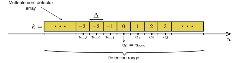
Figure 1: Multi-element detector array illustrating the standard coarse-graining geometry.

The standard model of coarse graining describes, for example, the typical projective measurements performed with an array of adjacent, rectangular detectors. A conventional example of such an apparatus is the image sensor of a digital camera, for which the pixel size stands for the detection resolution whereas the length of the full sensor embodies the range of detection. In the current analysis, we shall consider a linear detector array along a single spatial dimension rather than the two-dimensional area of a typical image sensor, as illustrated in Fig. 1. The coarse-graining interval representing the detection window of the $k$-th pixel of the linear array is then:

$$\mathcal{R}_{k}:=\left(u_{\rm cen}+(k-\frac{1}{2})\Delta,u_{\rm cen}+(k+\frac{1}{2})\Delta\right],$$ (39)

where $\Delta$ is the detector or pixel size – also commonly referred to as the coarse-graining width or the bin width. Using the definition (39), the discretised outcomes $u_{k}$ represent the $u$ value of the center of the corresponding bin:

$$u_{k}=u_{\rm cen}+k\Delta.$$ (40)

The parameter $u_{\rm cen}$ sets the position of the central bin of the array, whose outcome label is $k=0$, yielding $u_{0}=u_{\rm cen}$. To illustrate the effect of the coarse-graining design on measured distributions, we plot in Fig. 2 coarse-grained distributions (blue bars) obtained using 3 different resolutions: $\Delta=2$ (left colum), $\Delta=1$ (central column) and $\Delta=1/2$ (right column). For each resolution, we plot two distinct distributions obtained using $u_{\rm cen}=0$ (top row) and $u_{\rm cen}=\Delta/2$ (bottom row). In other words, the coarse-graining bins of the distributions plotted at the bottom part of the figure are displaced by half a “pixel" in relation to the distributions at the top. Clearly, the distribution obtained using a fixed resolution is not unique, but the effect of small displacements (smaller than the bin width) gets less important as the resolution is increased. For comparison, the generating continuous distribution is plotted in red.

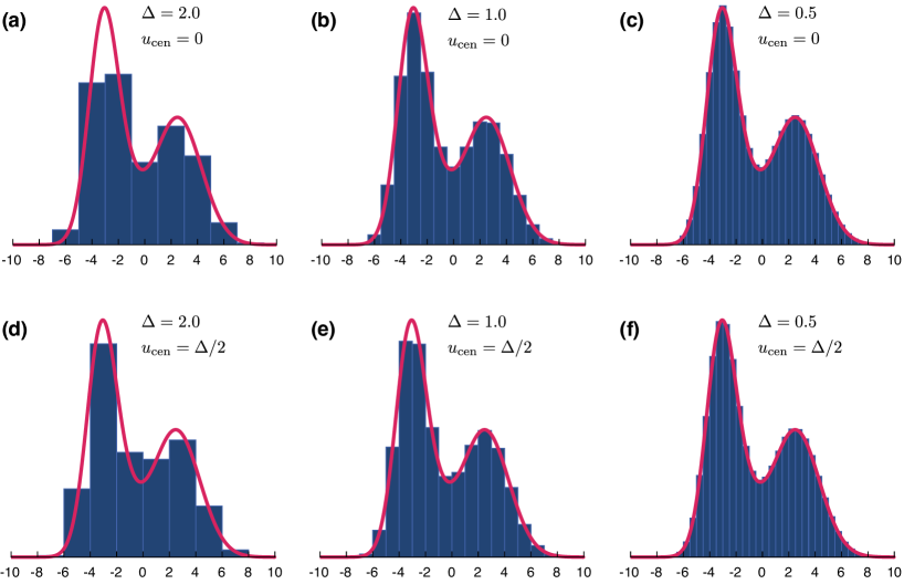
Figure 2: Coarse-grained distributions (blue bars) according to the standard model. The red solid line indicates the underlying continuous distribution used to generate the discretised versions. The used resolution $\Delta$ and positioning degree of freedom $u_{\rm cen}$ is indicated beside each distribution. For each resolution, two distinct distributions are shown, each of which associated with a different positioning of the coarse-graining bins.

We shall now use this model for standard coarse graining to explicitly define the discretised counterparts of the position and momentum operators given in Eq. (3).

$$\hat{u}_{\Delta} =\sum_{k}u_{k}\hat{C}_{k}^{(u)},$$ (41a)

$$\hat{v}_{\delta} =\sum_{l}v_{l}\hat{C}_{l}^{(v)},$$ (41b)

where the projector $\hat{C}_{k}$ is defined in Eq.(37) (with $\hat{C}_{l}^{(v)}$ having an equivalent definition for $\hat{v}$ measurements), and we used $\Delta$ ($\delta$) as the detection resolution for $\hat{u}$ ($\hat{v}$) measurements. According to the definition in Eq.(35), as a result of the the coarse-grained measurement of $\hat{u}$ and $\hat{v}$ we obtain the discrete probabilities, ${\rm p}^{(u)}_{\Delta,k}$ and ${\rm p}^{(v)}_{\delta,l}$.The discrete variances associate with these discrete probabilities are:

$$\sigma_{P_{\Delta}^{(u)}}^{2} =\sum_{k}u_{k}^{2}\;{\rm p}_{\Delta,k}^{(u)}-\left(\sum_{k}u_{k}\;{\rm p}_{\Delta,k}^{(u)}\right)^{2},$$ (42a)

$$\sigma_{P_{\delta}^{(v)}}^{2} =\sum_{l}v_{l}^{2}\;{\rm p}_{\delta,l}^{(v)}-\left(\sum_{l}v_{l}\;{\rm p}_{\delta,l}^{(v)}\right)^{2},$$ (42b)

where we define the set of discrete probabilities:

$$P_{\Delta}^{(u)}:=\{{\rm p}_{\Delta,k}^{(u)}\}\;\;\;\mbox{and}\;\;\;P_{\delta}^{(v)}:=\{{\rm p}_{\delta,k}^{(v)}\}.$$ (43)

One can see from the definitions (42) that if the bin widths $\Delta$ and $\delta$ are such that ${\rm p}_{\Delta,k}^{(u)}$ and ${\rm p}_{\delta,l}^{(v)}$ are sufficiently close to unity for for some value of $k$ and $l$, we have $\sigma_{P_{\Delta}^{(u)}}^{2},\sigma_{P_{\delta}^{(v)}}^{2}\longrightarrow 0$. Thus, naive application of any of the variance-based URs given in section 2.1 would indicate a false violation of a UR. It has been shown in Ref. Rudnicki, Ł. et al. (2012) that the same argument applies to discretized versions of entropic URs, such as those of section 2.2. Thus, proper treatment of standard coarse-grained measurements is essential in order to take advantage of the practical application of URs in QIT and quantum physics in general. In section 5 we show how this can be done.

4.1.2 Periodic Coarse Graining

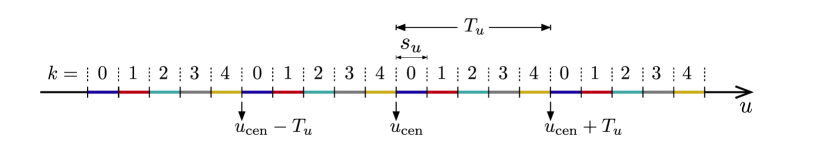
Figure 3: Periodic coarse-graining design with $d=T_{u}/s_{u}=5$ detection outcomes. The parameter $T_{u}$ is the periodicity in which bins of size $s_{u}$ are arranged.

A distinct model of coarse graining discussed in the literature Tasca et al. (2018); Paul et al. (2018) is refereed to as periodic coarse graining (PCG). In this model, the partition of the whole set of real numbers $\mathbb{R}$ is performed in a periodic manner, leading to a finite number $d$ of subsets $\mathcal{R}_{k}$, with $k=0,\cdots,d-1$. The resulting discretization utilizes the index $k$ as a direct label for the detection outcomes, in a similar fashion to what is usually defined for finite-dimensional quantum systems. The subsets $\mathcal{R}_{k}$ are defined as Tasca et al. (2018):

$$\mathcal{R}_{k}:=\left\{u\in\mathbb{R}\,|\,u_{\rm cen}+ks_{u}\leqslant u({\rm mod}\,T_{u})<\ u_{\rm cen}+(k+1)s_{u}\right\},$$ (44)

where $s_{u}$ plays the role of a bin width similar to the resolution $\Delta$ used for the standard coarse graining. In the definition (44), bins of size $s_{u}$ are arranged periodically with the parameter $T_{u}$ representing the period, as illustrated in Fig. 3 for the particular design using $d=T_{u}/s_{u}=5$ detection outcomes. It is important to notice that this coarse graining design do not distinguish detections in distinct bins associated with the same detection outcome $k$ (ranging from $0$ to $4$ in Fig. 3). For example, a detection within any bin colored in red in Fig. 44 would lead to the same detection outcome $k=1$.

An interesting feature of the PCG model is that the number of detection outcomes is utterly adjustable by the choice of the parameters $T_{u}$ and $s_{u}$, regardless of the chosen detection range. For instance, doubling the range of detection allows one to design PCG measurement using twice as much periods in its design, while maintaining the same number $d=T_{u}/s_{u}$ of detection outcomes. As with the standard model, the reference coordinate $u_{\rm cen}$ sets the center of the detection range also for the PCG design. Using the subset definition given in Eq. (44), we can explicitly write the projector operators, Eq. (37), for the PCG model as

$$\hat{\Pi}^{(u)}_{k}=\int_{\mathcal{R}_{k}}|u\rangle\langle u|du=\sum_{n\in\mathbb{Z}}\int_{u_{\rm cen}+ks_{u}+nT_{u}}^{u_{\rm cen}+(k+1)s_{u}+nT_{u}}|u\rangle\langle u|du,$$ (45)

where we extend the sum in $n$ over $\mathbb{Z}$ without loss of generality, assuming that Eq. (34) is satisfied. Analogously, we also define the PCG projective operators over the conjugate variable $v$:

$$\hat{\Pi}^{(v)}_{l}=\int_{\mathcal{R}_{l}}|v\rangle\langle v|dv=\sum_{n\in\mathbb{Z}}\int_{v_{\rm cen}+ls_{v}+nT_{v}}^{v_{\rm cen}+(l+1)s_{v}+nT_{v}}|v\rangle\langle v|dv,$$ (46)

where we define $s_{v}$ and $T_{v}$ as the bin width and periodicity used in the PCG measurements of $v$.

4.2 Mutual unbiasedness in coarse-grained measurements

If a quantum system is described as an eigenstate of a given observable, the measurement outcomes of a complementary observable are completely unbiased: each one of them occurring with equal probability, $1/d$, where $d$ is the dimension of the quantum system’s Hilbert space. This unbiasedness relation is an important feature of quantum mechanics with no classical counterpart, and is usually cast in terms of the basis vectors constituting the eigenstates of two (or more) complementary observables. To be more precise, two orthonormal bases $\{|a_{k}\rangle\}$ and $\{|b_{l}\rangle\}$ are said to be mutually unbiased if and only if $|\langle a_{k}|b_{l}\rangle|^{2}=1/d$ for all $k,l=0,\cdots,d-1$ Durt et al. (2010). The observation of unbiased measurement outcomes is customary in experiments with finite dimensional quantum systems. Not only routine, measurements in mutually unbiased bases (MUB) constitute a key procedure in a number of quantum information processing tasks, such as verification of cryptographic security Coles et al. (2017), certification of quantum randomness Vallone et al. (2014), detection of quantum correlations Spengler et al. (2012); Krenn et al. (2014); Erker et al. (2017) and tomographic reconstruction of quantum states Fernández-Pérez et al. (2011); Giovannini et al. (2013).

Mutual unbiasedness is also extendable to continuous variables quantum systems Weigert and Wilkinson (2008), for which conjugate bases $\{|u\rangle\}$ and $\{|v\rangle\}$ satisfy $|\langle u|v\rangle|^{2}=1/2\pi\hbar$, i.e., the overlap of the basis vectors $|u\rangle$ and $|v\rangle$ is independent (no bias) of their eigenvalues, $u$ and $v$. For CV systems, nevertheless, this relation is rather a theoretical definition than an experimentally observable fact, since the experimentalist has neither the capability to prepare nor to measure the (infinitely squeezed) eigenstates of the $\hat{u}$ and $\hat{v}$. Instead, both the preparation and measurement procedures are limited to the finite resolution of the experimental apparatus. As discussed previously in this section, measurements of a CV degree of freedom render discretized, coarse-grained outcomes whose probabilities, Eq. (35), are provided by a coarse-graining model described by the projective operators given in Eq. (37). These coarse-grained probabilities obtained experimentally do not in general preserve the mutual unbiasedness complied by the underlying continuous variables.

To elaborate the issue, let us consider sets of projectors $\{\hat{C}^{(u)}_{k}\}$ and $\{\hat{C}^{(v)}_{l}\}$ defining coarse-graining measurements in the complementary domains $u$ and $v$ of a continuous variable quantum system $\hat{\rho}$. We assume measurement designs providing a number $d$ of outcomes in each domain. In this scenario, the requirement for mutual unbiasedness is thus that the coarse-grained probabilities for measurements of one variable are evenly spread between all discretized outcomes whenever the quantum state is localized with respect to the coarse graining applied to its conjugate variable (and vice-versa). The subtlety in this requirement is the (infinite) degeneracy of normalizable quantum states that can be localized with respect to the chosen coarse graining. To emphasize this degeneracy, we refer to the outcome probabilities, Eq. $\eqref{P_k}$, with explicit dependency on the quantum state in order to mathematically phrase the condition for mutual unbiasedness in coarse-grained CV: the outcomes of $\{\hat{C}^{(u)}_{k}\}$ and $\{\hat{C}^{(v)}_{l}\}$ are mutually unbiased if for all quantum states $\hat{\rho}$ and $k_{0},l_{0}=0,\cdots,d-1$ we have Tasca et al. (2018):

$${\rm p}^{(u)}_{k}(\hat{\rho})=\delta_{k_{0}k}\hskip 7.22743pt\Rightarrow\hskip 7.22743pt{\rm p}^{(v)}_{l}(\hat{\rho})=d^{-1},$$ (47a)

$${\rm p}^{(v)}_{l}(\hat{\rho})=\delta_{l_{0}l}\hskip 7.22743pt\Rightarrow\hskip 7.22743pt{\rm p}^{(u)}_{k}(\hat{\rho})=d^{-1},$$ (47b)

where, again, we stress that ${\rm p}^{(u)}_{k}(\hat{\rho})={\rm Tr}(\hat{\rho}\hat{C}^{(u)}_{k})$ and ${\rm p}^{(v)}_{l}(\hat{\rho})={\rm Tr}(\hat{\rho}\hat{C}^{(v)}_{l})$, as in Eq. (35).

Having formulated the conditions for mutual unbiasedness, Eqs. (47), it is easy to perceive that the adjacent, rectangular subsets defining the standard coarse graining [Eq. (39)] will not lead to unbiased measurement outcomes. Any CV distribution localized in a single coarse-graining bin (for example in the $u$ variable) generates a probability density that decays in the Fourier domain (the $v$ variable) along the adjacent bins within the detection range. This decay generates a non constante coarse-grained distribution that, by definition, is biased. Furthermore, the number $d$ of detection outcomes in the standard design depends directly on the selected detection range, as well as on the chosen resolution. As a consequence, even though a particular localized distribution could lead to approximately unbiased coarse-grained outcomes in the Fourier domain, an extended detection range would increase the number of outcomes, thus spoiling the unbiasedness.

It is thus evident that in order to retrieve unbiased outcomes from coarse-grained measurement, a more contrived coarse-graining design is needed. As it turns out, it was shown in Ref. Tasca et al. (2018) that the PCG design exactly fulfils the requirements for unbiased measurements of finite cardinality stated in Eqs (47). A relation between the periodicities $T_{u}$ and $T_{v}$ used in the PCG of the conjugate variables $u$ and $v$ was analytically derived as a single condition for unbiased coarse-grained measurements:

$$\frac{T_{u}T_{v}}{2\pi\hbar}=\frac{d}{m},\hskip 14.45377ptm\in\mathbb{N}\hskip 14.45377pt{\rm s}.t.\hskip 14.45377pt\forall_{n=1,\cdots,d-1}\hskip 7.22743pt\frac{mn}{d}\notin\mathbb{N}.$$ (48)

The unbiasedness condition stated in Eq. (48) establishes infinite possibilities for the pair of periodicities $T_{u}$ and $T_{v}$ that can be used to design the mutually unbiased pair of PCG measurements defined in Eqs. (45) and (46), respectively. For instance, the simplest and most important case is the condition with $m=1$, since it is valid for all $d$ and provides the best trade-off between experimentally accessible periodicities: $T_{u}T_{v}=(2\pi\hbar)d$. Conditions with $m>1$ are also possible but are not general since they depend on the chosen number of outcomes $d$ Tasca et al. (2018). For example, for $d=4$, valid conditions are found using $m(\textrm{mod}\,d)=1,3$ whereas for $d=5$, valid conditions are found using $m(\textrm{mod}\,d)=1,2,3,4$. Importantly, the case with $m(\textrm{mod}\,d)=0$ is always excluded, since in this case the PCG projectors describe commuting sets, $\left[\hat{\Pi}^{(u)}_{k},\hat{\Pi}^{(v)}_{l}\right]=0$, $\forall$ $k,l$ Aharonov et al. (1969); Busch and Lahti (1986); Reiter and Thirring (1989). In other words a joint eigenstate of the product $\hat{\Pi}^{(u)}_{k}\hat{\Pi}^{(v)}_{l}$ existis for all $k$ and $l$ whenever $T_{u}T_{v}=2\pi\hbar/c$ with $c\in\mathbb{N}$ Rudnicki et al. (2016). It is also interesting to note that using the periodicity definition from the PCG design ($T=ds$), it is possible to write the unbiasedness condition given in Eq. (48) in alternative, equivalent ways:

$$(a)\,T_{u}T_{v}=\frac{2\pi\hbar}{m}d,\hskip 14.45377pt(b)\,T_{u}s_{v}=\frac{2\pi\hbar}{m},\hskip 14.45377pt(c)\,s_{u}T_{v}=\frac{2\pi\hbar}{m},\hskip 14.45377pt(d)\,s_{u}s_{v}=\frac{2\pi\hbar}{m}\frac{1}{d}.$$ (49)

Finally, in Ref. Paul et al. (2018) these results were generalized for PCG measurements applied to an arbitrary pair of phase space variables other than the conjugate pair formed by position and momentum. What is more, a triple of unbiased PCG measurements was also shown to exist for rotated phase space variables, along the same lines as the demonstration of a MUB triple in the continuous regime done in Ref. Weigert and Wilkinson (2008). Experimental demonstrations of unbiased PCG measurements were also carried out in Refs. Tasca et al. (2018); Paul et al. (2018), both of them utilizing the transverse spatial variables of a paraxial light field.

5 UR for coarse-grained observables

A kind of a paradigm shift in the theory of uncertainty relations was brought by the observation that everything can be efficiently characterized solely by means of probability distributions. As a result, tools known from information theory, such as information entropy, Fisher information and other measures, came into play. Additionally, the notion of uncertainty for discrete systems could better be captured that way. Since products of variances calculated for observables such as the spin are bounded in a state-dependent manner (so that the ultimate lower bound typically assumes the trivial value of $0$), information entropies provide an attractive alternative Deutsch (1983). Written already in the Rényi form,

$$H_{\alpha}\left[P\right]=\frac{1}{1-\alpha}\ln\sum_{k}[{\rm p}_{k}]^{\alpha},$$ (50)

the above equation is a discrete counterpart of Eq. (25), which corresponds to the discrete counterpart of Eq.(21) when $\alpha=1$.

In the finite-dimensional case given by an arbitrary state $\hat{\rho}$ acting on a $d$-dimensional Hilbert space $\mathcal{H}$, and a pair of non-degenerate, non-commuting observables, $\hat{A}$ and $\hat{B}$, one usually defines the probabilities:

$${\rm p}_{i}^{(A)}=\left\langle a_{i}\right|\hat{\rho}\left|a_{i}\right\rangle,\qquad{\rm p}_{j}^{(B)}=\left\langle b_{j}\right|\hat{\rho}\left|b_{j}\right\rangle.$$ (51)

By $\left|a_{i}\right\rangle$ and $\left|b_{j}\right\rangle$, $i,j=1,\ldots,d$ we denote the eigenstates of the operators associated with both observables. Disctrete entropic URs for the above probability distributions are of the general form

$$H_{\alpha}\left[P^{(A)}\right]+H_{\beta}\left[P^{(B)}\right]\geq B_{\alpha\beta}\left(\mathbf{U}\right),$$ (52)

with $\mathbf{U}\in\mathcal{U}\left(d\right)$ being a unitary matrix with matrix elements $\mathbf{U}_{ij}=\left\langle a_{i}\left|b_{j}\right\rangle\right.\!$. We denote $P^{(A)}:=\{{\rm p}_{i}^{(A)}\}$ and $P^{(B)}:=\{{\rm p}_{j}^{(B)}\}$ again with $i,j=1,\ldots,d$.

The first entropic uncertainty relation for discrete variables comes from Deutsch Deutsch (1983), who for $\alpha=1=\beta$ found the lower bound $B_{11}^{\textrm{D}}=-2\ln C$, with $C=\left(1+\sqrt{c_{1}}\right)/2$ and $c_{1}=\max_{i,j}\left|U_{ij}\right|^{2}$. A substantially more renowned Maassen–Uffink (MU) bound Maassen and Uffink (1988) derived in 1988, is $B_{\alpha\beta}^{\textrm{MU}}=-\ln c_{1}$. This bound is however valid only for the conjugate parameters $1/\alpha+1/\beta=2$. Very recently, a plethora of new results Korzekwa et al. (2014); Friedland et al. (2013); Puchała et al. (2013); Coles and Piani (2014); Rudnicki et al. (2014); Bosyk et al. (2014); Zozor et al. (2014); Kaniewski et al. (2014); Puchała et al. (2018) improving the celebrated MU bound has been obtained. In particular, an approach based on the notion of majorization (suitable from the perspective of resource theories and quantum thermodynamics Brandão et al. (2015)) provides a significant qualitative novelty Friedland et al. (2013); Puchała et al. (2013); Rudnicki et al. (2014); Puchała et al. (2018), which will also be touched upon in this section.

In this review we are concerned with the case in which continuous probability distributions $P_{u}\left(u\right)$ and $P_{v}\left(v\right)$ are replaced (viz. they were measured this way) by their discrete counterparts ($k,l\in\mathbb{Z}$). According to the discussion in Section 4 we can use the definitions in Eq.(35) and (39), and the condition in Eq.(33), to write the discrete probabilities:

$${\rm p}_{\Delta,k}^{(u)}=\int_{\left(k-1/2\right)\Delta}^{\left(k+1/2\right)\Delta}dy\;P_{u}\left(y\right),\qquad{\rm p}_{\delta,l}^{(v)}=\int_{\left(l-1/2\right)\delta}^{\left(l+1/2\right)\delta}dy\;P_{v}\left(y\right),$$ (53)

with $k\in\mathcal{Z}_{k}\subset\mathbb{Z}$. In the following we describe a series of URs for these discrete probabilities that are known as coarse-grained URs, derived in Bialynicki-Birula (1984, 2006); Rudnicki, Ł. et al. (2012); Rudnicki et al. (2012). These are the coarse-grained counterpart of the Heisenberg, Shannon entropy and Rényi entropy URs in Eqs.(8),(20) and (24) respectively. Here, we will closely follow the treatment in Rudnicki, Ł. et al. (2012); Rudnicki et al. (2012), however, before we start we give a short historical overview and discuss a path towards extensions going beyond CCOs.

The idea that generic quantum uncertainty could be quantified by the sum of Shannon entropies evaluated for discretized position and momentum probability distributions for the first time appeared in the contribution by Partovi Partovi (1983). He also derived the first coarse-grained UR which in the form is reminiscent to the Deutsch bound for finite-dimensional systems Deutsch (1983). Both bounds Deutsch (1983); Partovi (1983) were obtained by means of a direct optimization, independently applied to every logarithmic contribution. Symmetry in developments of the URs for finite-dimensional and coarse-grained systems happened to be much deeper as the second coarse-grained result, by Bialynicki-Birula Bialynicki-Birula (1984), is a counterpart of the MU bound Maassen and Uffink (1988). The former result is an application of the continuous variant of the Shannon entropy UR (so the $L_{p}$-$L_{q}$ norm inequality by Beckner Beckner (1975)) supported by the Jensen inequality for convex functions, while the MU bound is a direct consequence of the Riesz theorem for the $l_{p}$-$l_{q}$ norms. Note that relatively often, integration limits in (53) were chosen as ”from $k\Delta$ to $(k+1)\Delta$” and ”from $l\delta$ to $(l+1)\delta$”, however this choice causes a formal pathology in the limit of infinite coarse graining Rudnicki (2011). Thus, sticking to terminology of Eq. (39), in theory it is better to avoid borderline settings for the position of the central bin, i.e. $u_{\textrm{cen}}=\Delta/2$.

To briefly report later developments, one shall mention that Partovi reconsidered the problem he had posed several years ago, pioneering applications of majorizaiton techniques Partovi (2011). Also Schürmann and Hoffmann Schürmann and Hoffmann (2009) discussed the Shannon entropy UR from the perspective of the integral equation associated to it, while the first author conjectured an improvement (later mentioned in detail) which agrees with his numerical tests Schürmann (2012). Finally, we mention (without details) an erroneous improvement of Bialynicki-Birula (2006) by Wilk and Wlodarczyk Wilk and Włodarczyk (2009); Bialynicki-Birula and Rudnicki (2010), mainly devoted to the case of the Tsallis entropy.

Although originally the URs were derived for CCOs, $\hat{u}$ and $\hat{v}$, here we show which of the URs in Rudnicki, Ł. et al. (2012); Rudnicki et al. (2012) can be valid also for operators $\hat{u}$ and $\hat{v}$ that are arbitrary linear combinations of all positions and momenta of the $n-$bosonic modes like the ones defined in Eq.(3), viz. operators that are not necessarily CCOs. In the general case, we stress that there is always a unitary metaplectic transformation, $\hat{U}_{\mathbf{S}}$, that connects $\hat{u}$ and $\hat{v}$, viz. $\hat{v}=\hat{U}_{\mathbf{S}}^{\dagger}\hat{u}\hat{U}_{\mathbf{S}}$. However, this metaplectic transformation is not necessarily a $\pi/2$ rotation, which would be the case if $\hat{u}$ and $\hat{v}$ were CCOs. In order to see this, we first define two sets of operators $({\bf\hat{u}},{\bf\hat{u}}^{\prime})^{T}=(\hat{u}=\hat{u}_{1},\ldots,\hat{u}_{n},\hat{u}_{1}^{\prime},\ldots,\hat{u}_{n}^{\prime})^{T}=\sqrt{\gamma}\,\tilde{\mathbf{S}}\,{\bf\hat{x}}$ and $({\bf\hat{v}},{\bf\hat{v}}^{\prime})^{T}=(\hat{v}=\hat{v}_{1},\ldots,\hat{v}_{n},\hat{v}_{1}^{\prime}\ldots,\hat{v}_{n}^{\prime})^{T}=\sqrt{\gamma}\,{\mathbf{S}^{\prime}}\,{\bf\hat{x}}$, where $\tilde{\mathbf{S}}$ and $\mathbf{S}^{\prime}$ are some matrices belonging to the symplectic group $Sp(2n,\mathbb{R})$, with the only restriction that the first rows of $\tilde{\mathbf{S}}$ and $\mathbf{S}^{\prime}$ correspond to the real coefficients ${\bf d}$ and ${\bf d}^{\prime}$ in Eq.(5), respectively, which define the operators $\hat{u}$ and $\hat{v}$ in Eq.(3). Due to the properties of symplectic matrices, all the pairs $\hat{u}_{i}$ and $\hat{u}_{j}^{\prime}$, and also $\hat{v}_{i}$ and $\hat{v}_{j}^{\prime}$, satisfy CCRs, viz. $[\hat{u}_{i},\hat{u}_{j}^{\prime}]=i\hbar\gamma\delta_{ij}$ and $[\hat{v}_{i},\hat{v}_{j}^{\prime}]=i\hbar\gamma\delta_{ij}$ with $i,j=1,\ldots,n$. But it is immediate to see that $({\bf\hat{v}},{\bf\hat{v}}^{\prime})^{T}=\mathbf{S}({\bf\hat{u}},{\bf\hat{u}}^{\prime})^{T}$ where the matrix $\mathbf{S}:={\mathbf{S}}^{\prime}\tilde{\mathbf{S}}^{-1}$ is a generic symplectic matrix. Then the Stone-von-Neumann theorem guarantees that the change $({\bf\hat{u}},{\bf\hat{u}}^{\prime})^{T}\rightarrow({\bf\hat{v}},{\bf\hat{v}}^{\prime})^{T}$ is unitarily implementable by a metaplectic transformation $\hat{U}_{\mathbf{S}}$ Dutta et al. (1995). In particular we have $\hat{U}_{\mathbf{S}}^{\dagger}\,\hat{u}\,\hat{U}_{\mathbf{S}}=(\mathbf{S}\,{\bf\hat{x}})_{1}=:\hat{v}$.

5.1 URs proved only for CCOs

The key concept behind the treatment of coarse-grained URs in Rudnicki, Ł. et al. (2012); Rudnicki et al. (2012) is the introduction of the piece-wise continuous probability density functions:

$$Q_{\Delta,u}(u):=\sum_{k\in\mathcal{Z}_{k}}{\rm p}^{(u)}_{\Delta,k}\;D_{\Delta}(u,u_{k})\;\;\;\mbox{and}\;\;\;Q_{\delta,v}(v):=\sum_{l\in\mathcal{Z}_{l}}{\rm p}^{(v)}_{\delta,l}\;D_{\delta}(v,v_{l}),$$ (54)

where $D_{\Delta}(u,u_{k})$ and $D_{\delta}(v,v_{l})$ are called the histogram functions (HF) with $u_{k}$ (and $v_{l}$ in an analogous way) defined in Eq. (40). Generically, these functions are defined such that they are normalized in each bin:

$$\int_{(k-1/2)\Delta}^{(k+1/2)\Delta}D_{\Delta}(u,u_{k})\;du=1\;\;\;\mbox{and}\;\;\;\int_{(l-1/2)\Delta}^{(l+1/2)\Delta}D_{\Delta}(v,v_{l})\;dv=1,$$ (55)

and approach the Dirac delta distribution for infinitesimal bin size:

$$\lim_{\Delta\rightarrow 0}D_{\Delta}(u,u_{k})=\delta(u-u_{k})\;\;\;\mbox{and}\;\;\;\lim_{\delta\rightarrow 0}D_{\delta}(v,v_{l})=\delta(v-v_{l}).$$ (56)

Therefore, in the limit $\mathcal{Z}_{k},\mathcal{Z}_{l}\rightarrow\mathbb{Z}$ and $\Delta,\delta\rightarrow 0$ we have $Q_{\Delta,u}(u)\rightarrow P_{u}(u)$ and $Q_{\delta,v}(v)\rightarrow P_{v}(v)$. We shall stress here that the HF can, in general, have any functional form as long as it is non-negative, normalized and fulfills Eq. (56). However, the most common histogram function is the rectangular HF:

$$D^{R}_{\Delta}(u,u_{k}):=\left\{\begin{matrix}1/\Delta&\mbox{for $u\in\left((k-\frac{1}{2})\Delta,(k+\frac{1}{2})\Delta\right]$}\\ 0&\mbox{otherwise.}\\ \end{matrix}\right.,$$ (57)

with an equivalent definition for $D^{R}_{\delta}(v,v_{l})$. In Fig.2 we show an example of coarse-grained probability distributions functions $Q_{\Delta,u}(u)$ (the area beneath these functions are displayed in full) using rectangular histogram functions and for different size bins $\Delta$.

Here, we generalise the results in Rudnicki, Ł. et al. (2012); Rudnicki et al. (2012) through the following expression that will be justified later:

$$h_{\alpha}[Q_{\Delta,u}]+h_{\beta}[Q_{\delta,v}]\geq\ln\left(\frac{\pi\hbar|\gamma|\;e^{h_{\alpha}[D_{\Delta}]-\ln\Delta+h_{\beta}[D_{\delta}]-\ln\delta}}{\varepsilon_{\alpha}(\Gamma/4)}\right),$$ (58)

with $1/\alpha+1/\beta=2$ and $1/2\leq\alpha\leq 1$. To simplify the notation we define the function:

$$\varepsilon_{\alpha}\left(x\right):=\min\left\{\alpha^{\frac{1}{2-2\alpha}}\beta^{\frac{1}{2-2\beta}},\frac{1}{2}R^{2}_{00}\left(x,1\right)\right\},$$ (59)

where $R_{00}(x,y)$ denotes one of the radial prolate spheroidal wave functions of the first kind Abramowitz and Stegun (1964), and introduce the joint coarse-graining parameter $\Gamma=\Delta\delta/(\hbar|\gamma|)$. We stress that (58) involves the differential Rényi entropies of the piece-wise continuous distributions defined in Eqs. (54).

Let us see how the results in Bialynicki-Birula (1984, 2006); Bialynicki-Birula and Rudnicki (2011); Rudnicki, Ł. et al. (2012); Rudnicki et al. (2012) can be derived from Eq.(58). First, we observe that the Rényi entropies of rectangular HFs, for every values of $\alpha$ and $\beta$, are:

$$h_{\alpha}[D^{R}_{\Delta}]=\ln\Delta\;\;\;\mbox{and}\;\;\;h_{\beta}[D^{R}_{\Delta}]=\ln\delta,$$ (60)

so Eq.(58) reduces to:

$$h_{\alpha}[Q_{\Delta,u}]+h_{\beta}[Q_{\delta,v}]\geq\ln\left(\frac{\pi\hbar|\gamma|}{\varepsilon_{\alpha}(\Gamma/4)}\right).$$ (61)

If we perform the limit $\Gamma/4\rightarrow 0$ in Eq.(61), we have $(1/2)R^{2}_{00}\left(\Gamma/4,1\right)\rightarrow 1/2$, and considering that $1/e<\alpha^{\frac{1}{2-2\alpha}}\beta^{\frac{1}{2-2\beta}}\leq 1/2$ when $1/2<\alpha\leq 1$ (see Fig.(4)) we recover the Rényi-entropy UR in Eq.(24) and when $\alpha=1$ the Shannon UR in Eq.(20).

Now, we can decompose the differential Rényi entropies in the left hand side of Eq.(58) as (see Appendix A):

$$h_{\alpha}[Q_{\Delta,u}]=H_{\alpha}\left[P_{\Delta}^{(u)}\right]+h_{\alpha}\left[D_{\Delta}\right]\;\;\;\mbox{and}\;\;\;h_{\beta}[Q_{\delta,v}]=H_{\beta}\left[P_{\delta}^{(v)}\right]+h_{\beta}\left[D_{\delta}\right],$$ (62)

where we denote the set of discrete probabilities appearing in Eq.(53) as $P_{\Delta}^{(u)}:=\{{\rm p}_{\Delta,k}^{(u)}\}$ and $P_{\delta}^{(v)}:=\{{\rm p}_{\delta,k}^{(v)}\}$, respectively. Note that, for pdfs with bounded support, the Rényi entropy is maximized for the uniform distribution Lassance (2017), so we always have: $h_{\alpha}\left[D_{\Delta}\right]\leq\ln(\Delta)$ and $h_{\beta}\left[D_{\delta}\right]\leq\ln(\delta)$. If we apply the result Eq.(62) to the inequality (58) we recover the result proved in Ref. Rudnicki et al. (2012) for the discrete entropies:

$$H_{\alpha}[P_{\Delta}^{(u)}]+H_{\beta}[P_{\delta}^{(v)}]\geq\ln\left(\frac{\pi}{\varepsilon_{\alpha}(\Gamma/4)\Gamma}\right).$$ (63)

This is the coarse-grained version of the Rényi entropy UR in Eq.(24). We shall also emphasize, as the title of this subsection suggests, that the demonstration of the URs (63) presented in Ref. Rudnicki et al. (2012) uses explicitly the fact that $\hat{u}$ and $\hat{v}$ form a CCO pair. Therefore, the UR in Eq.(58) is, in principle, valid only for CCO pairs, since it can be obtained from Eq.(63) by adding $h_{\alpha}\left[D_{\Delta}\right]+h_{\beta}\left[D_{\delta}\right]$ to both sides, and using Eq.(62).

The discrete Rényi entropy is always positive, and we have

$$\lim_{\Gamma\rightarrow+\infty}\ln\left(\frac{\pi}{\Gamma\varepsilon_{\alpha}(\Gamma/4)}\right)=\lim_{\Gamma\rightarrow+\infty}\ln\left(\frac{\pi}{\frac{1}{2}\Gamma R^{2}_{00}\left(\frac{\Gamma}{4},1\right)}\right)=0,$$ (64)

with the last line being valid because $\lim_{x\rightarrow\infty}(2x/\pi)R_{00}^{2}(x,1)=1$. This results show that the coarse-grained UR in Eq.(63) is non-trivially satisfied for an arbitrary (even very large) values of the coarse-graining widths. However, this desired property is not enjoyed by the UR

$$H_{\alpha}[P_{\Delta}^{(u)}]+H_{\beta}[P_{\delta}^{(v)}]\geq\ln\left(\frac{\pi}{\alpha^{\frac{1}{2-2\alpha}}\beta^{\frac{1}{2-2\beta}}\Gamma}\right),$$ (65)

first derived in Bialynicki-Birula (2006). This UR corresponds to Eq.(63) in the coarse-grained regime $\Gamma/4\lesssim 1.79$ in which $\varepsilon_{1}(\Gamma/4)=1/e$. Obviously, this is not a mere coincidence, as Eq. (63) subsumes (65). This is clearly visible inside the definition of $\varepsilon$ which involves the minimum of two different bounds. When $\Gamma/4>1.79$ the lower bound in Eq.(65) is negative so this UR is trivially satisfied, since the discrete entropy is always non-negative.

Figure 4: In panel (a) the full line is the graph of the function $f(\alpha)=\alpha^{\frac{1}{2-2\alpha}}\beta^{\frac{1}{2-2\beta}}$, with $0<\alpha\leq 1$, and where $\beta(\alpha)=\alpha/(2\alpha-1)$ that stems from the condition $1/\alpha+1/\beta=2$. The horizontal dashed line is drawn to indicate the limit $\lim_{\alpha\rightarrow 1}f(\alpha)=1/e$. In panel (b) we plot the behaviour of $g(y)=(1/2)R_{00}(y,1)$ as a function of $y:=\Delta\delta/(4\hbar|\gamma|)$. Although $g(y)$ is shown in the range $0\leq y\leq 50$, it is important to note that $g(y)$ is continuous monotonically decreasing function in the positive real axis such $\lim_{y\rightarrow\infty}g(y)=0$.

From the above considerations we can obtain an UR for the variances, $\sigma^{2}_{Q_{\Delta,u}}$ and $\sigma^{2}_{Q_{\delta,v}}$ , if we set $\alpha=1$ in Eq.(58) and use the inequality (22):

$$\ln(2\pi e\sigma_{Q_{\Delta,u}}\sigma_{Q_{\delta,v}})\geq h[Q_{\Delta,u}]+h[Q_{\delta,v}]\geq\ln\left(\frac{\pi\hbar|\gamma|\;e^{h[D_{\Delta}]-\ln\Delta+h[D_{\delta}]-\ln\delta}}{\varepsilon_{1}(\Gamma/4)}\right),$$ (66)

where $h[\cdot]$ stands for the Shannon entropy. Now, we can use the decompositions:

$$\sigma_{Q_{\Delta,u}}^{2}=\sigma^{2}_{P_{\Delta}^{(u)}}+\sigma^{2}_{D_{\Delta}}\;\;\;\mbox{and}\;\;\;\sigma_{Q_{\delta,v}}^{2}=\sigma^{2}_{P_{\delta}^{(v)}}+\sigma^{2}_{D_{\delta}},$$ (67)

where the variances of the discrete probability distributions were defined in Eq.(42), while $\sigma^{2}_{D_{\Delta}}$ and $\sigma^{2}_{D_{\delta}}$, are the variances of the generic HFs. Therefore, applying the above splitting to Eq.(66) we arrive at the lower bound Rudnicki et al. (2012):

$$\left(\sigma^{2}_{P_{\Delta}^{(u)}}+\sigma^{2}_{D_{\Delta}}\right)\left(\sigma^{2}_{P_{\delta}^{(v)}}+\sigma^{2}_{D_{\delta}}\right)\geq\frac{\hbar^{2}\gamma^{2}}{4}\frac{e^{2(h[D_{\Delta}]-\ln\Delta+h[D_{\delta}]-\ln\delta-1)}}{\varepsilon^{2}_{1}(\Gamma/4|\gamma|)}.$$ (68)

When the HF are rectangular, and in the coarse-grained regime $\Gamma/(4|\gamma|)\lesssim 1.79$ where $\varepsilon_{1}(\Gamma/4|\gamma|)=1/e$, we recover the UR Rudnicki, Ł. et al. (2012):

$$\left(\sigma^{2}_{P_{\Delta}^{(u)}}+\frac{\Delta^{2}}{12}\right)\left(\sigma^{2}_{P_{\delta}^{(v)}}+\frac{\delta^{2}}{12}\right)\geq\frac{\hbar^{2}\gamma^{2}}{4},$$ (69)

where we have used the fact that in this case

$$\sigma^{2}_{D^{R}_{\Delta}}=\frac{\Delta^{2}}{12}\;\;\;\mbox{and}\;\;\;\sigma^{2}_{D^{R}_{\delta}}=\frac{\delta^{2}}{12}.$$ (70)

Both (68) and (69) are the coarse-grained versions of the Heisenberg UR in Eq.(8). It is important to emphasize that (69) cannot be obtained by the simple substitution $\sigma^{2}_{P_{u}}\rightarrow\sigma^{2}_{P_{\Delta}^{(u)}}$ and $\sigma^{2}_{P_{v}}\rightarrow\sigma^{2}_{P_{\delta}^{(v)}}$ done inside the Heisenberg UR.

Although both $\sigma^{2}_{D_{\Delta}}$ and $\sigma^{2}_{D_{\delta}}$ are the variances of a generic HF, viz. $D_{\Delta}(u,u_{k})$ and $D_{\delta}(v,v_{k})$ for any value of $k$, it is interesting to associate them to the respective central bins, namely those that contain the mean value of the probability distributions $P_{u}$ and $P_{v}$. By doing this, together choosing the origins of the coordinates in the middle of the central bin, we can see that the variances $\sigma^{2}_{P_{\Delta}^{(u)}}$ and $\sigma^{2}_{P_{\delta}^{(v)}}$ are free from contributions associated with the statistics relevant for the central bins. Thus, if the widths of the coarse graining increase in the measurement of $\hat{u}$ and $\hat{v}$, the respective central bin-widths grow, so that the variances $\sigma^{2}_{P_{\Delta}^{(u)}}$ and $\sigma^{2}_{P_{\delta}^{(v)}}$ only involve contributions from the tails of the probability distributions $Q_{\Delta,u}$ and $Q_{\delta,v}$. Therefore, for large coarse grainings, the variances $\sigma^{2}_{D_{\Delta}}$ and $\sigma^{2}_{D_{\delta}}$ become more important in the inequalities (68) and (69). Thus, in the regime when:

$$\Gamma \geq \pi e\Rightarrow\Gamma\geq\frac{\pi}{\varepsilon_{1}(\Gamma/4|\gamma|)}\Rightarrow\Gamma^{2}\geq\frac{1}{4}\frac{e^{2(h[D_{\Delta}]+h[D_{\delta}])}}{e^{2}\sigma^{2}_{D_{\Delta}}\sigma^{2}_{D_{\delta}}\varepsilon^{2}_{1}(\Gamma/4|\gamma|)}\Rightarrow$$ (71)

$$\Rightarrow \sigma^{2}_{D_{\Delta}}\sigma^{2}_{D_{\delta}}\geq\frac{\hbar^{2}|\gamma|^{2}}{4}\frac{e^{2(h[D_{\Delta}]-\ln\Delta+h[D_{\delta}]-\ln\delta-1)}}{\varepsilon^{2}_{1}(\Gamma/4|\gamma|)}$$

both (68) and (69) are satisfied trivially. Note, that in Eq.(71) we have used the relation $4\pi^{2}\geq e^{2(h[D_{\Delta}]+h[D_{\delta}])}/e^{2}\sigma^{2}_{D_{\Delta}}\sigma^{2}_{D_{\delta}}>0$ which can be obtained from the inequality in Eq.(22).

However, Eq.(68) is only the starting point for the second construction, proposed in Rudnicki et al. (2012), that is free from the above limitation, and cannot be trivially satisfied. This improved UR reads:

$$K\left(\frac{\sigma^{2}_{P_{\Delta}^{(u)}}}{\Delta^{2}}\right)K\left(\frac{\sigma^{2}_{P_{\delta}^{(v)}}}{\delta^{2}}\right)\geq\frac{\pi^{2}}{\Gamma^{2}\varepsilon^{2}_{1}(\Gamma/4)},$$ (72)

where $K(t)$ is implicitly defined as

$$K(t):=\frac{\exp[2t{\cal M}^{-1}(t)]}{\erf^{2}\left(\sqrt{{\cal M}^{-1}(t)}/2\right)},$$

with $\erf(x):=(2/\sqrt{\pi})\int_{0}^{x}e^{-y^{2}}dy$ being the error function and ${\cal M}^{-1}(t)$ denoting the inverse of the invertible function

$${\cal M}(y):=\frac{\exp(-y/4)}{2\sqrt{\pi t}\erf(\sqrt{t}/2)}.$$

The idea behind derivation of the coarse-grained UR in Eq.(72) is the following. Let us rewrite Eq.(68) in the form:

$$\xi(h[D_{\Delta}],\sigma^{2}_{D_{\Delta}},h[D_{\delta}],\sigma^{2}_{D_{\delta}}):=\frac{\left(\sigma^{2}_{P_{\Delta}^{(u)}}+\sigma^{2}_{D_{\Delta}}\right)\left(\sigma^{2}_{P_{\delta}^{(v)}}+\sigma^{2}_{D_{\delta}}\right)}{e^{2(h[D_{\Delta}]+h[D_{\delta}]-1)}}\geq\frac{1}{4\Gamma^{2}\varepsilon^{2}_{1}(\Gamma/4)}.$$

Now the function $\xi$ is supposed to be minimized, however, because the Shannon entropy $h[D_{\Delta}]$ ($h[D_{\delta}]$) is interrelated with (bounded by a function of) the variance $\sigma^{2}_{D_{\Delta}}$ ($\sigma^{2}_{D_{\delta}}$) the minimization needs to be performed in two steps. For fixed values of the variances $\sigma^{2}_{D_{\Delta}}$ and $\sigma^{2}_{D_{\delta}}$, the function $\xi$ achieves its minimum when the Shannon entropies $h[D_{\Delta}]$ and $h[D_{\delta}]$ are maximized with respect to the functional form of the HFs, $D_{\Delta}$ and $D_{\delta}$. As already stated, the HFs are constrained by the requirement of the fixed value for both variance. The form of the HF with maximum Shannon entropy Rudnicki et al. (2012) is a Gaussian with support restricted to the central bin and whose variance is an appropriate function of $\sigma^{2}_{D_{\Delta}}$ ($\sigma^{2}_{D_{\delta}}$). Therefore, for this optimal HF its Shannon entropy $h[D^{op}_{\Delta}]$ ($h[D^{op}_{\delta}]$) is only a function of the variance $\sigma^{2}_{D_{\delta}}$ ($\sigma^{2}_{D_{\delta}}$), thus we have $G(\sigma^{2}_{D_{\Delta}},\sigma^{2}_{D_{\delta}})=\xi(h[D^{op}_{\Delta}],\sigma^{2}_{D_{\Delta}},h[D^{op}_{\delta}],\sigma^{2}_{D_{\delta}})$. The second step is a direct minimization of $G(\sigma^{2}_{D_{\Delta}},\sigma^{2}_{D_{\delta}})$, which results in the left hand side product in Eq.(72).

According to the discussion above Eq.(71) the coarse-grianed UR in Eq.(72) has no contributions from the statistics corresponding to the central bin. In the limit when $\Delta,\delta\rightarrow 0$ we recover the Heisenberg UR in Eq(8) thanks to the identities Rudnicki et al. (2012)

$$\lim_{\Delta\rightarrow 0}\Delta^{2}K\left(\frac{\sigma^{2}_{P_{\Delta}^{(u)}}}{\Delta^{2}}\right)=\sigma^{2}_{P_{u}}\lim_{y\rightarrow 0}\frac{1}{{\cal M}(y)}\frac{\exp(2y{\cal M}(y))}{\erf^{2}\left({\sqrt{y}/2}\right)}=2\pi e\sigma^{2}_{P_{u}}.$$ (73)

In the opposite limit of infinite coarse graining, viz $\Delta,\delta\rightarrow\infty$, we have $\sigma_{P_{\Delta}^{(u)}}^{2},\sigma_{P_{\delta}^{(v)}}^{2}\longrightarrow 0$ and

$$\overbrace{\lim_{\sigma_{P_{\Delta}^{(u)}}^{2}\rightarrow 0}K\left(\frac{\sigma^{2}_{P_{\Delta}^{(u)}}}{\Delta^{2}}\right)}^{=1}\overbrace{\lim_{\sigma_{P_{\delta}^{(v)}}^{2}\rightarrow 0}K\left(\frac{\sigma^{2}_{P_{\delta}^{(v)}}}{\delta^{2}}\right)}^{=1}\geq\overbrace{\lim_{\Gamma\rightarrow\infty}\frac{\pi^{2}}{\Gamma^{2}\varepsilon^{2}_{1}(\Gamma/4)}}^{=1}.$$ (74)

It is important to note that since

$$\frac{\pi^{2}}{\Gamma^{2}\varepsilon^{2}_{1}(\Gamma/4)}>1,$$ (75)

whenever both $\Delta$ and $\delta$ are finite, it is forbidden to set $\sigma_{P_{\Delta}^{(u)}}^{2}$ and $\sigma_{P_{\delta}^{(v)}}^{2}$ as simultaneously equal to zero, as it would contradict the coarse-grained UR (72). This means that any quantum state (pure or mixed) cannot be localised in both observables $\hat{u}$ and $\hat{v}$ that are CCOs. In other words, the associated probability distributions cannot simultaneously have compact support.

This remarkable conclusion somehow threatens the scientific program to recover classical mechanics solely from coarse-grained averaging, physically originating from the finite-precision of the observations Ballentine (1998); Kofler and Brukner (2007); Kofler and Časlav Brukner (2007). Indeed, quantum features can be observed in the measurement of $\hat{u}$ and $\hat{v}$ irrespective of the precision of the detectors. However, for very large coarse-graining widths the variances $\sigma_{P_{\Delta}^{(u)}}^{2}$ and $\sigma_{P_{\delta}^{(v)}}^{2}$ are dominated by the contributions from the tails of the $P_{\Delta}^{(u)}$ and $P_{\delta}^{(v)}$. Thus, as these probabilities are likely very small, they would be particularly susceptible to statistical fluctuations and it would in general require very long acquisition times to collect the sufficient amount of data necessary to verify the UR (72) in the regime of extremely large coarse graining.

5.2 URs valid for general observables, $\hat{u}$ and $\hat{v}$, defined in Eq.(3).

If we let $\alpha=1$ in Eq.(58), use rectangular HFs such that Eq.(60) is valid and restrict the size of the involved bins such that $\varepsilon_{1}(\Gamma/4|\gamma|)=1/e$ — this is the regime of the coarse graining when $\Gamma/4\lesssim 1.79$ — we obtain the simplified coarse-grained UR of the form:

$$h[Q_{\Delta,u}]+h[Q_{\delta,v}]\geq\ln\left(\pi e\hbar|\gamma|\right).$$ (76)

Because the coarse-grained UR in Eq.(58) was derived only for CCOs, $\hat{u}$ and $\hat{v}$, a priori it is not clear why the above UR could remain valid also for generalized observables defined in Eq.(3). This fact, however, can be proved with the help of the Shannon-entropy UR (20), that has properly been extended to the desired observables, and the inequalities:

$$h[Q_{\Delta,u}]\geq h[P_{u}]\;\;\;\mbox{and}\;\;\;h[Q_{\delta,v}]\geq h[P_{v}],$$ (77)

whose detailed derivation based on the Jensen inequality is relegated to Appendix B. Passing to the discrete entropies we find the coarse-grained UR:

$$H[P_{\Delta}^{(u)}]+H[P_{\delta}^{(v)}]\geq\ln\left(\frac{\pi e}{\Gamma}\right),$$ (78)

which looks the same as the one derived in Bialynicki-Birula (1984) for CCOs. Here, the validity of this UR has been extended for any observables $\hat{u}$ and $\hat{v}$ as defined in Eq.(3). Also, following the same arguments that lead from Eq.(66) to the UR in Eq.(69) we can see that the UR for the discrete variances is also valid for general $\hat{u}$ and $\hat{v}$ as defined in Eq.(3).

To briefly summarize, entropic uncertainty relations for coarse-grained probability distributions were almost only considered for position and momentum variables. As far as we know, the only exceptions are given in Refs. Huang (2011); Guanlei et al. (2009). However, as we have shown here, the generalization of entropic URs for differential probabilities associated with general observables $\hat{u}$ and $\hat{v}$, which are linear combinations of position and momentum, can be done in many cases. However, in each case a careful analysis should be carried out to verify that the related coarse-grained URs are also valid for these generalised operators. Here, we have done this only in the simple cases.

5.3 Coarse-grained URs merged with the majorization approach

In Rudnicki (2015) the coarse-grained scenario has been discussed with the help of the results obtained in Friedland et al. (2013); Puchała et al. (2013); Rudnicki et al. (2014), namely the majorization-based approach to quantification of uncertainty. To say it briefly, a majorization relation $x\prec y$ between two arbitrary $d$-dimensional probability distributions means that for every $n\leq d$ the inequality $\sum_{k=1}^{n}x_{k}^{\downarrow}\leq\sum_{k=1}^{n}y_{k}^{\downarrow}$ holds, with an equality (normalization) for $n=d$. Traditionally, by “$\downarrow$” we denote the decreasing order, so that $\bigl{(}x^{\downarrow}\bigr{)}{}_{k}\geq\bigl{(}x^{\downarrow}\bigr{)}{}_{l}$, for all $k\leq l$. The Rényi entropy (and also others, such as the Tsallis entropy) is Schur-concave, which implies $H_{\alpha}\left[x\right]\geq H_{\alpha}\left[y\right]$ whenever $x\prec y$.

In the context of coarse-grained probability distributions it was conceptually simpler to consider the so-called direct-sum majorization introduced in Rudnicki et al. (2014). An advantage of the majorization approach is that it covers a regime of ($\alpha,\beta$) parameters, $\beta=\alpha$ to be precise, which in some way is perpendicular to the conjugate choice $1/\alpha+1/\beta=2$. In Rudnicki (2015) an infinite hierarchy of majorization vectors, depending on a single parameter $\Gamma=\Delta\delta/\hbar$, has been derived. The discussion is conducted for CCOs, thus one can easily recognize the dimensionless $\Gamma$ parameter as those which appears in all previous URs [[FT: with $\gamma=1$]].

The main result, namely a family of lower bounds denoted as $\mathcal{R}_{\alpha}^{(n)}\left(\Delta\delta/\hbar\right)$ for $n=2,\dots,\infty$, has been presented in Eq. (27) from Rudnicki (2015), however, we refrain from providing its detailed construction here. It seems enough to say that the bound in question is a function of $R^{2}_{00}\left(j_{0}\Gamma/4,1\right)$ with $j_{0}$ being certain positive integers. In other words, in spirit, the majorization bound is close to that derived in Rudnicki et al. (2012) and extensively discussed above. A comparison of the new bound and (63) for $\alpha=1=\beta$ — the only value of both parameters for which the involved bounds describe the same situation — showed that $\mathcal{R}_{1}^{(3)}$ outperforms (63) in the regime when the $R_{00}$-term does contribute to $\varepsilon_{1}$.

Asymptotic behavior of the new and previous coarse-grained bounds shows that for $\alpha=1=\beta$ and large $\Gamma$, all $\mathcal{R}_{1}^{(n)}$ bounds improve (63) by a divergent factor $\Gamma/4$. Moreover, the typical behavior of discrete majorization bounds has been confirmed in the coarse-grained setting. In the discrete case, the majorization relations almost surely dominate the MU bound, with an exception being a small neighborhood of the point for which the unitary matrix $\mathbf{U}$ is the Fourier matrix. The analog of the Fourier matrix in the coarse-grained scenario is the continuous limit $\Gamma\rightarrow 0$. This probably intuitive fact has been rigorously shown by means of the asymptotics of $\mathcal{R}_{1}^{(\infty)}$ for small $\Gamma$, which is equal to $-\frac{1}{2}\ln\Gamma$.

5.4 Other coarse-grained URs

At the very end of this long section we would like to touch upon few coarse-grained URs which go beyond the standard position-momentum conjugate pair. First of all, Bialynicki-Birula also provided his major Shannon entropy UR in the case of angle and angular momentum Bialynicki-Birula (1984), as well as to the variables on the sphere Bialynicki-Birula and Madajczyk (1985). Coarse graining in these physical settings is only relevant for the periodic CVs (angle on a circle and two angles on a sphere), as the conjugate variables are discrete (though infinite dimensional).

Also, the coarse-grained scenario has been developed Furrer et al. (2014) in relation to the memory-assisted UR Berta et al. (2010) relevant for quantum key distribution. The result, even though non-trivial, differs from Eq. (63) in a similar fashion as the MU bound differs from the UR in the presence of quantum memory by Berta et al Berta et al. (2010).

Going in a completely different direction, Rastegin Rastegin (2017) in his recent contribution proposed an extension of (65) to the case of a modified CCR, which assumes the form $[\hat{x},\hat{p}]=i\hbar(1+\beta\hat{p}^{2})$. The parameter $\beta$ is related to the so-called minimal length predicted by certain variants of string theory and similar approaches.

Last but not least, some of us have very recently derived an inequality (see Eqs. 9-12 from Tasca et al. (2018)), which could be understood as an UR (valid for CCOs) in the setting relevant for periodic coarse graining discussed in section 4.1.2. As this UR involves additional averaging of ${\rm p}^{(x)}_{k}(\hat{\rho})$ and ${\rm p}^{(p)}_{l}(\hat{\rho})$ defined below Eq. (47) with respect to the positioning degrees of freedom, we do not provide further details of this construction encouraging the interested reader to consult Tasca et al. (2018).

6 Applications of coarse-grained measurements and coarse-grained Uncertainty Relations

As discussed above, when detecting the position and momentum of particles such as photons or individual atoms, coarse-grained measurements are not just necessary but can be much more practical. In this regard, URs that deal with coarse-grained measurements can be useful for a number of applications, such as those discussed in section 3.

In Ref. Schneeloch et al. (2013) EPR-steering was tested for discrete distributions of measurements made from standardized binning on the two-photon state produced from spontaneous parametric down-conversion, using a coarse-grained version of the EPR-steering criteria of Ref. Walborn et al. (2011). Bi-dimensional steering was observed for sample sizes ranging from $8\times 8$ to $24\times 24$, representing a considerable reduction in measurement overhead when compared with the quasi-continuous measurements reported in Ref. Walborn et al. (2011), which sampled about 100 data points per cartesian direction (about $10^{4}$ total measurements) to evaluate entropic EPR-steering criteria of continuous variables.

The pitfalls of applying the usual entanglement criteria for continuous variables to coarse-grained measurements was shown in Ref. Tasca et al. (2013), where it was demonstrated that this can lead to false-positive identifications of entanglement, such that the separability criteria based on uncertainty relations discussed in section 3 can be (falsely) violated even for separable states. To show how binned data should be properly handled, a coarse-grained UR was used, along with the PPT argument to properly identify entanglement experimentally in a system of spatially-entangled photons. In particular, a variance criteria based on (69) was tested for the global operators defined in equations (29) and (30). It was also shown that coarse-grained entropic entanglement criteria, for example based on inequality (58) ($\alpha=\beta=1$) applied to operators (29) and (30), can be superior to coarse-grained variance based criteria, identifying entanglement when variance criteria do not, even for the case of Gaussian states. This is due to the fact that the coarse-grained probability distributions functions such as those shown in figure 2 are not Gaussian functions, even when the quantum state under investigation is Gaussian.

Standard coarse graining has been studied in the context of quantum state reconstruction of single and two-mode Gaussian states, and the quantum to classical transition Park et al. (2014). Two scenarios were considered: direct reconstruction of the covariance matrix alone, and full reconstruction of the state using maximum likelihood estimation. The reconstructed coarse-grained functions were compared to those of Gaussian states subject to thermal squeezed reservoirs, indicating that in this context coarse graining does not produce a thermalized (decohered) Gaussian state.

The work mentioned above considered standard coarse graining, as described in section 4.1. In some cases it is interesting to consider different models, such as that of periodic coarse graining described in section 4.1.2. The mutual unbiasedness of periodic coarse graining described in section 4.2 has been tested experimentally for two Tasca et al. (2018) and even three Paul et al. (2018) phase-space directions. It was shown that mutual unbiasedness appears when the appropriate bin widths of the two or three conjugate variables are chosen. Periodic coarse graining has also been used in the detection of spatial correlations of photon pairs from SPDC Tasca et al. (2018). Using a novel entanglement criteria based on the UR for characteristic functions Rudnicki et al. (2016), it was possible to identify entanglement with as few as $2\times 2$ measurements in position and momentum (8 total), representing a considerable reduction in measurement overhead.

Simple binary binning of homodyne measurements has been proposed as a means to test dichotomic Bell’s inequalities in CV systems, while allowing for high detection efficency Gilchrist et al. (1998, 1999); Munro (1999); García-Patrón et al. (2004). Other types of non-standard coarse graining have been proposed as a means to violate Bell’s inequality using homodyne measurements on non-Gaussian states Wenger et al. (2003). Though it was shown that one could achieve maximal violation in principle, exotic non-Gaussian states are required. In Ref. Tasca et al. (2009) it was shown that imperfect binning could result in false violations of Bell’s inequalities, and even in violations of Cirelson’s bound for quantum Bell correlations.

A closely related subject to periodic coarse graining of CVs is that of the so called modular variables Aharanov and Rohrlich (2005); Vernaz-Gris et al. (2014); Ketterer et al. (2016), for which phase-space variables $u$ are rewritten as $u=n_{u}\ell+\bar{u}$, where $n_{u}$ is the integer component and $\bar{u}$ the modular component, such that $0\leq\bar{u}<\ell$. Here $\ell$ is a scaling parameter of appropriate dimension. For two CCOs, such as $\hat{x}$ and $\hat{p}$ for example, the integer operator of one observable–say–$\hat{n}_{x}$ and the modular operator of the other observable–$\hat{\bar{p}}$ satisfy URs that closely resemble those of the angle and angular momentum variables Bialynicki-Birula (1984). The modular variable construction was first introduced by Aharanov et al. Aharonov et al. (1969); Aharanov and Rohrlich (2005) as a method to identify non-locality in quantum mechanics. Since then, a number of interesting applications have been developed. Variance-based URs for the modular variable construction were proposed as a method to identify a novel type of squeezing, as well as entanglement in pairs of atoms Gneiting and Hornberger (2011). This entanglement criteria was used in Refs. Carvalho et al. (2012), along with one based on entropic uncertainty relations, to identify spatial entanglement of photon pairs that have passed through multiple slit apertures. Application to multiple-photon states was studied in Ref. Barros et al. (2015). It is worth noting that in this case the usual CV entanglement criteria as discussed in section 3 are incapable of detecting entanglement. Modular variables have been proposed as a way to test for the Greenberger-Horne-Zeilinger paradox in CV systems Massar and Pironio (2001), as well as quantum contextuality Plastino and Cabello (2010); Asadian et al. ; Laversanne-Finot et al. (2017) and as a method to construct algebras resembling that of discrete systems Vernaz-Gris et al. (2014); Asadian et al. (2016); Ketterer et al. (2016).

7 Conclusion

Uncertainty relations play an important role in quantum physics, which is two-fold: on the one hand they have historically represented the difference between classical and quantum physics, while on the other hand they are a tool that can be used to identify and even quantify interesting quantum properties. Beginning with the seminal work of Heisenberg in 1927, a number of uncertainty relations have been developed for continuous variable quantum systems. However, in a realistic experimental setting, one never has access to the infinite dimensional spectrum associated to these observables. Thus, coarse graining is imposed by the detection apparatus to account for the measurement precision and range.

Here we have provided a review of a number of quantum mechanical uncertainty relations tailored specifically to coarse-grained measurement of continuous quantum observables. Our aim was to survey the state-of-the-art of the subject, from both the theoretical advances to experimental application of coarse-grained uncertainty relations.

A number of interesting open questions remain. First, it would be interesting to see the generalization of all the coarse-grained URs presented here for pairs of observables that are connected by general unitary metaplectic transformations. Second, one can consider applying coarse graining to URs not mentioned explicitely here, such as the triple variance product criteria Weigert and Wilkinson (2008); Paul et al. (2016), UR for characteristic functions Rudnicki et al. (2016), among others, as well the plethora of moment inequalities arising from tests for non-classicality Shchukin et al. (2005); Ryl et al. (2015) and entanglement Shchukin and Vogel (2005); Agarwal and Biswas (2005); Hillery and Zubairy (2006). Third, and more important, a deep discussion of the role of coarse-grained URs within the scientific program to recover classical mechanics solely from coarse-grained averaging should be developed. We hope that this review encourage this discussion.

8 Conclusions

Appendix A

Following Rudnicki et al. (2012) we aim to prove the decomposition in Eq.(62). To this end it is enough to discuss the case of $\hat{u}$ since the proof for $\hat{v}$ looks the same. We can write:

$$h_{\alpha}[Q_{\Delta,u}] = \frac{1}{1-\alpha}\ln\left(\int_{-\infty}^{\infty}du\;[Q_{\Delta,u}(u)]^{\alpha}\right)=\frac{1}{1-\alpha}\ln\left(\sum_{k\in{\mathcal{Z}}_{k}}\int_{{\mathcal{R}}_{k}}du\;[Q_{\Delta,u}(u)]^{\alpha}\right)$$ (79)

$$= \frac{1}{1-\alpha}\ln\left(\sum_{k\in{\mathcal{Z}}_{k}}\left[p^{(u)}_{\Delta,k}\right]^{\alpha}\int_{{\mathcal{R}}_{k}}du\;[D_{\Delta}(u,u_{k})]^{\alpha}\right),$$

where we use the fact that the function $Q_{\Delta,u}(u)$ in the interval $\mathcal{R}_{k}$ is equal to ${\rm p}^{(u)}_{\Delta,k}\;D_{\Delta}(u,u_{k})$. Now, because the shape of the HF, $D_{\Delta}(u,u_{k})$, is the same for all values of $k$, the integral $\int_{{\mathcal{R}}_{k}}du\;[D_{\Delta}(u,u_{k})]^{\alpha}$ does not depend on $k$. Therefore, we can write:

$$h_{\alpha}[Q_{\Delta,u}]=\frac{1}{1-\alpha}\ln\left(\sum_{k\in{\mathcal{Z}}_{k}}\left[p^{(u)}_{\Delta,k}\right]^{\alpha}\right)+\frac{1}{1-\alpha}\ln\left(\int_{{\mathcal{R}}_{k}}du\;[D_{\Delta}(u,u_{k})]^{\alpha}\right),$$ (80)

that corresponds to the decomposition in Eq.(62).

Appendix B

Here, we prove the inequalities in Eq.(77). As before, is enough to consider the single case relevant for the variable $u$. What we do in the next few lines, we actually closely follow the treatment presented in Bialynicki-Birula and Rudnicki (2011). First we define the mean value within the $k$th histogram bin:

$$\expectationvalue{\ldots}_{k}:=\frac{1}{\Delta}\int_{(k-1/2)\Delta}^{(k+1/2)\Delta}\ldots du.$$ (81)

Then, because the function $f(x)=x\ln(x)$ is convex we can apply Jensen’s inequality Cover and Thomas (2006) to obtain,

$$\expectationvalue{P_{u}\ln P_{u}}_{k}\geq\expectationvalue{P_{u}}_{k}\ln\expectationvalue{P_{u}}_{k}.$$ (82)

Now we can use the definition in Eq.(53), multiply both sides by $-1$ and sum over $k\in{\cal Z}_{k}$:

$$-\sum_{k\in{\cal Z}_{k}}{\rm p}_{\Delta,k}^{(u)}\ln{\rm p}_{\Delta,k}^{(u)}+\left(\sum_{k\in{\cal Z}_{k}}{\rm p}_{\Delta,k}^{(u)}\right)\ln(\Delta)\geq-\sum_{k\in{\cal Z}_{k}}\int_{(k-1/2)\Delta}^{(k+1/2)\Delta}P_{u}(u)\ln P_{u}(u)\;du.$$ (83)

After using the condition in Eq.(36), the definition of the discrete Shannon entropy $H[P_{\Delta}^{(u)}]:=-\sum_{k\in{\cal Z}_{k}}{\rm p}_{\Delta,k}^{(u)}\ln{\rm p}_{\Delta,k}^{(u)}$, the decomposition in Eq.(62) with $\alpha=1$ and $h[D^{R}_{\Delta}]=\ln\Delta$, and the definition of the differential Shannon entropy in Eq.(21) we obtain:

$$h[Q_{\Delta,u}]:=H[P_{\Delta}^{(u)}]+\ln\Delta\geq h[P_{u}],$$ (84)

which is the desired result.

References

- Wheeler and Zurek (1983) Wheeler, J.A.; Zurek, W.H., Eds. Quantum Theory and Measurement; Princeton University Press: Princeton, NJ, 1983.
- Scully et al. (1991) Scully, M.O.; Englert, B.G.; Walther, H. Quantum optical tests of complementarity. Nature 1991, 351, 111.
- Kim et al. (2000) Kim, Y.H.; Kulik, S.; Shih, Y.; Scully, M. Delayed Choice Quantum Eraser. Phys. Rev. Lett. 2000, 84, 1.
- Bertet et al. (2001) Bertet, P.; Osnaghi, S.; Rauschenbeutel, A.; Nogues, G.; Auffeves, A.; Brune, M.; Raimond, J.M.; Haroche, S. A complementarity experiment with an interferometer at the quantum-classical boundary. Nature 2001, 411, 166–170.
- Walborn et al. (2002) Walborn, S.P.; Cunha, M.O.T.; Pádua, S.; Monken, C.H. Double-slit quantum eraser. Phys. Rev. A 2002, 65, 0338.
- Mandel (1991) Mandel, L. Coherence and indistinguishability. Opt. Lett. 1991, 16, 1882.
- Englert (1996) Englert, B.G. Fringe Visibility and Which-Way Information: An Inequality. Phys. Rev. Lett. 1996, 77, 2154.
- Ozaktas et al. (2001) Ozaktas, H.M.; Zalevsky, Z.; Kutay, M.A. The Fractional Fourier Transform: with Applications in Optics and Signal Processing; John Wiley and Sons Ltd: New York, 2001.
- Coles et al. (2017) Coles, P.J.; Berta, M.; Tomamichel, M.; Wehner, S. Entropic uncertainty relations and their applications. Reviews of Modern Physics 2017, 89, 0848–58.
- Braunstein and van Loock (2005) Braunstein, S.L.; van Loock, P. Quantum information with continuous variables. Rev. Mod. Phys. 2005, 77, 513.
- Adesso et al. (2014) Adesso, G.; Ragy, S.; Lee, A.R. Continuous Variable Quantum Information: Gaussian States and Beyond. Open Syst. Inf. Dyn. 2014, 21, 1440001.
- Bialynicki-Birula and Rudnicki (2011) Bialynicki-Birula, I.; Rudnicki, Ł., Entropic Uncertainty Relations in Quantum Physics. In In Chapter 1 of: Statistical Complexity: Applications in Electronic Structure; Sen, K., Ed.; Springer Netherlands: Dordrecht, 2011; pp. 1–34.
- Wehner and Winter (2010) Wehner, S.; Winter, A. Entropic uncertainty relations—a survey. New Journal of Physics 2010, 12, 025009.
- Sperling and Vogel (2009) Sperling, J.; Vogel, W. Verifying continuous-variable entanglement in finite spaces. Phys. Rev. A 2009, 79, 052313.
- Willard (1902) Willard, J. Elementary Principles in statistical mechanics; Scribner’s sons: New York, 1902.
- Ehrenfest and Ehrenfest (1912) Ehrenfest, P.; Ehrenfest, T. Begriffliche Grundlagen der Statistischen Auffassung in der Mechanik; B. G. Teubner: Leipzig, Germany, 1912.
- Ehrenfest and Ehrenfest (1990) Ehrenfest, P.; Ehrenfest, T. The Conceptual Foundations of the Statistical Approach in Mechanics; Dover: New York, 1990.
- Mackey (1992) Mackey, M. Time’s Arrow: The Origins of Thermodynamical Behavior; Springer-Verlag: New York, 1992.
- Kofler and Brukner (2007) Kofler, J.; Brukner, i.c.v. Classical World Arising out of Quantum Physics under the Restriction of Coarse-Grained Measurements. Phys. Rev. Lett. 2007, 99, 180403.
- Kofler and Brukner (2008) Kofler, J.; Brukner, i.c.v. Conditions for Quantum Violation of Macroscopic Realism. Phys. Rev. Lett. 2008, 101, 090403.
- Raeisi et al. (2011) Raeisi, S.; Sekatski, P.; Simon, C. Coarse Graining Makes It Hard to See Micro-Macro Entanglement. Phys. Rev. Lett. 2011, 107, 250401.
- Wang et al. (2013) Wang, T.; Ghobadi, R.; Raeisi, S.; Simon, C. Precision requirements for observing macroscopic quantum effects. Phys. Rev. A 2013, 88, 062114.
- Jeong et al. (2014) Jeong, H.; Lim, Y.; Kim, M.S. Coarsening Measurement References and the Quantum-to-Classical Transition. Phys. Rev. Lett. 2014, 112, 010402.
- Rudnicki et al. (2012) Rudnicki, L.; Walborn, S.P.; Toscano, F. Optimal uncertainty relations for extremely coarse-grained measurements. Phys. Rev. A 2012, 85, 042115.
- Ray and van Enk (2013) Ray, M.R.; van Enk, S.J. Missing data outside the detector range. II. Application to time-frequency entanglement. Phys. Rev. A 2013, 88, 062327.
- Tasca et al. (2013) Tasca, D.S.; Rudnicki, L.; Gomes, R.M.; Toscano, F.; Walborn, S.P. Reliable Entanglement Detection under Coarse-Grained Measurements. Phys. Rev. Lett. 2013, 110, 210502.
- Tasca et al. (2009) Tasca, D.S.; Walborn, S.P.; Toscano, F.; Souto Ribeiro, P.H. Observation of tunable Popescu-Rohrlich correlations through postselection of a Gaussian state. Phys. Rev. A 2009, 80, 030101.
- Semenov and Vogel (2011) Semenov, A.A.; Vogel, W. Fake violations of the quantum Bell-parameter bound. Phys. Rev. A 2011, 83, 032119.
- Ray and van Enk (2013) Ray, M.R.; van Enk, S.J. Missing data outside the detector range: Continuous-variable entanglement verification and quantum cryptography. Phys. Rev. A 2013, 88, 042326.
- Bialynicki-Birula (1984) Bialynicki-Birula, I. Entropic Uncertainty Relations. Phys. Lett. 1984, 103 A, 253.
- Bialynicki-Birula (2006) Bialynicki-Birula, I. Formulation of the uncertainty relations in terms of the Rényi entropies. Phys. Rev. A 2006, 74.
- Rudnicki, Ł. et al. (2012) Rudnicki, Ł..; Walborn, S. P..; Toscano, F.. Heisenberg uncertainty relation for coarse-grained observables. EPL 2012, 97, 38003.
- Heisenberg (1927) Heisenberg, W. Über den anschaulichen Inhalt der quantentheoretischen Kinematik und Mechanik. Zeitschrift für Physik 1927, 43, 172–198.
- Busch et al. (2007) Busch, P.; Heinonen, T.; Lahti, P. Heisenberg’s uncertainty principle. Physics Reports 2007, 452, 155–176.
- Ozawa (2003) Ozawa, M. Universally valid reformulation of the Heisenberg uncertainty principle on noise and disturbance in measurement. Physical Review A 2003, 67, 042105.
- Ozawa (2004) Ozawa, M. Uncertainty relations for noise and disturbance in generalized quantum measurements. Annals of Physics 2004, 311, 350–416.
- Ozawa (2005) Ozawa, M. Universal uncertainty principle in the measurement operator formalism. Journal of Optics B: Quantum and Semiclassical Optics 2005, 7, S672–S681.
- Werner (2004) Werner, R.F. The Uncertainty Relation for Joint Measurement of Postion and Momentum. Quantum Info. Comput. 2004, 4, 546–562.
- Busch et al. (2004) Busch, P.; Heinonen, T.; Lahti, P. Noise and disturbance in quantum measurement. Physics Letters A 2004, 320, 261–270.
- Busch et al. (2013) Busch, P.; Lahti, P.; Werner, R.F. Proof of Heisenberg’s Error-Disturbance Relation. Physical Review Letters 2013, 111, 160405.
- Arthurs and Kelly (1965) Arthurs, E.; Kelly, J.L. On the Simultaneous Measurement of a Pair of Conjugate Observables. Bell System Technical Journal 1965, 44, 725–729.
- Arthurs and Goodman (1988) Arthurs, E.; Goodman, M.S. Quantum correlations: A generalized Heisenberg uncertainty relation. Physical Review Letters 1988, 60, 2447–2449.
- Ishikawa (1991) Ishikawa, S. Uncertainty relations in simultaneous measurements for arbitrary observables. Reports on Mathematical Physics 1991, 29, 257–273.
- Raymer (1994) Raymer, M. Uncertainty principle for joint measurement of noncommuting variables. American Journal of Physics 1994, 62, 986.
- Ozawa (2004) Ozawa, M. Uncertainty relations for joint measurements of noncommuting observables. Physics Letters A 2004, 320, 367–374.
- Tasca et al. (2011) Tasca, D.S.; Gomes, R.M.; Toscano, F.; Souto Ribeiro, P.H.; Walborn, S.P. Continuous-variable quantum computation with spatial degrees of freedom of photons. Phys. Rev. A 2011, 83, 052325.
- Dutta et al. (1995) Dutta, B.; Mukunda, N.; Simon, R. The real symplectic groups in quantum mechanics and optics. Pramana 1995, 45, 471–497.
- Kennard (1927) Kennard, E.H. Zur Quantenmechanik einfacher Bewegungstypen. Zeitschrift für Physik 1927, 44, 326–352.
- Weyl (1928) Weyl, H. Gruppentheorie und Quantenmechanik (Leipzig: S Hirzel) Weyl H 1950 The Theory of Groups and Quantum Mechanics, 1928.
- Robertson (1929) Robertson, H. The uncertainty principle. Physical Review 1929, 34, 163–164.
- Schrödinger (1930) Schrödinger, E. On Heisenberg’s Uncertainty Principle. Sitzungsber. Preuss. Akad. Wiss.(Proceedings of the Prussian Academy of Sciences), Phys. Math.Kl. 1930, 19, 296.
- Simon et al. (1994) Simon, R.; Mukunda, N.; Dutta, B. Quantum-noise matrix for multimode systems: U (n) invariance, squeezing, and normal forms. Physical Review A 1994.
- Solomon Ivan et al. (2012) Solomon Ivan, J.; Sabapathy, K.K.; Mukunda, N.; Simon, R. Invariant theoretic approach to uncertainty relations for quantum systems, 2012, [arXiv:1205.5132v1].
- Simon (2000) Simon, R. Peres-Horodecki Separability Criterion for Continuous Variable Systems. Phys. Rev. Lett. 2000, 84, 2726–2729.
- Huang (2011) Huang, Y. Entropic uncertainty relations in multidimensional position and momentum spaces. Phys. Rev. A 2011, 83, 052124.
- Shannon (1948) Shannon, C.E. A Mathematical Theory of Communication. Bell System Technical Journal 1948, 27, 379–423.
- Cover and Thomas (2006) Cover.; Thomas. Elements of Information Theory; John Wiley and Sons, 2006.
- Bialynicki-Birula and Mycielski (1975) Bialynicki-Birula, I.; Mycielski, J. Uncertainty Relations for Information Entropy in Wave Mechanics. Commun. Math. Phys. 1975, 44, 129.
- Beckner (1975) Beckner, W. Inequalities in Fourier Analysis. Annals of Mathematics 1975, 102, 159–182.
- Babenko (1961) Babenko, K.I. IAn inequality in the theory of Fourier integrals. Izv. Akad. Nauk SSSR Ser. Mat 1961, 25, 531–542.
- Hirschman (1957) Hirschman, I.I. A Note on Entropy. American Journal of Mathematics 1957, 79, 152–156.
- Guanlei et al. (2009) Guanlei, X.; Xiaotong, W.; Xiaogang, X. Generalized entropic uncertainty principle on fractional Fourier transform. Signal Processing 2009, 89, 2692 – 2697. Special Section: Visual Information Analysis for Security.
- Narcowich (1990) Narcowich, F.J. Geometry and uncertainty. J. Math. Phys. 1990, 31, 354–364.
- Slusher et al. (1985) Slusher, R.E.; Hollberg, L.W.; Yurke, B.; Mertz, J.C.; Valley, J.F. Observation of Squeezed States Generated by Four-Wave Mixing in an Optical Cavity. Phys. Rev. Lett. 1985, 55, 2409–2412.
- Shchukin et al. (2005) Shchukin, E.; Richter, T.; Vogel, W. Nonclassicality criteria in terms of moments. Phys. Rev. A 2005, 71, 011802.
- Vogel (2000) Vogel, W. Nonclassical States: An Observable Criterion. Phys. Rev. Lett. 2000, 84, 1849–1852.
- Richter and Vogel (2002) Richter, T.; Vogel, W. Nonclassicality of Quantum States: A Hierarchy of Observable Conditions. Phys. Rev. Lett. 2002, 89, 283601.
- Kiesel et al. (2009) Kiesel, T.; Vogel, W.; Hage, B.; DiGuglielmo, J.; Samblowski, A.; Schnabel, R. Experimental test of nonclassicality criteria for phase-diffused squeezed states. Phys. Rev. A 2009, 79, 022122.
- Ryl et al. (2015) Ryl, S.; Sperling, J.; Agudelo, E.; Mraz, M.; Köhnke, S.; Hage, B.; Vogel, W. Unified nonclassicality criteria. Phys. Rev. A 2015, 92, 011801.
- Reid and Drummond (1988) Reid, M.D.; Drummond, P.D. Quantum Correlations of Phase in Nondegenerate Parametric Oscillation. Phys. Rev. Lett. 1988, 60, 2731–2733.
- Reid (1989) Reid, M.D. Demonstration of the Einstein-Podolsky-Rosen paradox using nondegenerate parametric amplification. Phys. Rev. A 1989, 40, 913–923.
- Einstein et al. (1935) Einstein, A.; Podolsky, D.; Rosen, N. Can Quantum-Mechanical Description of Physical Reality Be Considered Complete? Phys. Rev. 1935, 47, 777.
- Ou et al. (1992) Ou, Z.Y.; Pereira, S.F.; Kimble, H.J.; Peng, K.C. Realization of the Einstein-Podolsky-Rosen paradox for continuous variables. Phys. Rev. Lett. 1992, 68, 3663–3666.
- Wiseman et al. (2007) Wiseman, H.M.; Jones, S.J.; Doherty, A.C. Steering, Entanglement, Nonlocality, and the Einstein-Podolsky-Rosen Paradox. Phys. Rev. Lett. 2007, 98, 140402.
- Jones et al. (2007) Jones, S.J.; Wiseman, H.M.; Doherty, A.C. Entanglement, Einstein-Podolsky-Rosen correlations, Bell nonlocality, and steering. Phys. Rev. A 2007, 76, 052116.
- Cavalcanti and Skrzypczyk (2017) Cavalcanti, D.; Skrzypczyk, P. Quantum steering: a review with focus on semidefinite programming. Rep. Prog. Phys. 2017, 80, 024001.
- Schrödinger (1935) Schrödinger, E. The Present Status of Quantum Mechanics. Naturwissenschaften 1935, 23, 807.
- Horodecki et al. (2009) Horodecki, R.; Horodecki, P.; Horodecki, M.; Horodecki, K. Quantum entanglement. Rev. Mod. Phys. 2009, 81, 865–942.
- Gühne and Tóth (2009) Gühne, O.; Tóth, G. Entanglement detection. Physics Reports 2009, 474, 1 – 75.
- Brunner et al. (2014) Brunner, N.; Cavalcanti, D.; Pironio, S.; Scarani, V.; Wehner, S. Bell nonlocality. Rev. Mod. Phys. 2014, 86, 419–478.
- Ji et al. (2015) Ji, S.W.; Lee, J.; Park, J.; Nha, H. Steering criteria via covariance matrices of local observables in arbitrary-dimensional quantum systems. Phys. Rev. A 2015, 92, 062130.
- Walborn et al. (2011) Walborn, S.P.; Salles, A.; Gomes, R.M.; Toscano, F.; Souto Ribeiro, P.H. Revealing Hidden Einstein-Podolsky-Rosen Nonlocality. Phys. Rev. Lett. 2011, 106, 130402.
- Schneeloch et al. (2013) Schneeloch, J.; Dixon, P.B.; Howland, G.A.; Broadbent, C.J.; Howell, J.C. Violation of Continuous-Variable Einstein-Podolsky-Rosen Steering with Discrete Measurements. Phys. Rev. Lett. 2013, 110, 130407.
- Reid (2000) Reid, M.D. Quantum cryptography with a predetermined key, using continuous-variable Einstein-Podolsky-Rosen correlations. Phys. Rev. A 2000, 62, 062308.
- Grosshans and Cerf (2004) Grosshans, F.; Cerf, N.J. Continuous-Variable Quantum Cryptography is Secure against Non-Gaussian Attacks. Phys. Rev. Lett. 2004, 92.
- Branciard et al. (2012) Branciard, C.; Cavalcanti, E.G.; Walborn, S.P.; Scarani, V.; Wiseman, H.M. One-sided device-independent quantum key distribution: Security, feasibility, and the connection with steering. Phys. Rev. A 2012, 85, 010301.
- Kogias et al. (2015) Kogias, I.; Skrzypczyk, P.; Cavalcanti, D.; Acín, A.; Adesso, G. Hierarchy of Steering Criteria Based on Moments for All Bipartite Quantum Systems. Phys. Rev. Lett. 2015, 115, 210401.
- Silberhorn et al. (2001) Silberhorn, C.; Lam, P.K.; Weiß, O.; König, F.; Korolkova, N.; Leuchs, G. Generation of Continuous Variable Einstein-Podolsky-Rosen Entanglement via the Kerr Nonlinearity in an Optical Fiber. Phys. Rev. Lett. 2001, 86, 4267–4270.
- Bowen et al. (2003) Bowen, W.P.; Schnabel, R.; Lam, P.K.; Ralph, T.C. Experimental Investigation of Criteria for Continuous Variable Entanglement. Phys. Rev. Lett. 2003, 90, 043601.
- D’Angelo et al. (2004) D’Angelo, M.; Kim, Y.H.; Kulik, S.P.; Shih, Y. Identifying Entanglement Using Quantum Ghost Interference and Imaging. Phys. Rev. Lett. 2004, 92, 233601.
- Howell et al. (2004) Howell, J.C.; Bennink, R.S.; Bentley, S.J.; Boyd, R.W. Realization of the Einstein-Podolsky-Rosen Paradox Using Momentum- and Position-Entangled Photons from Spontaneous Parametric Down Conversion. Phys. Rev. Lett. 2004, 92, 210403.
- Tasca et al. (2009) Tasca, D.S.; Walborn, S.P.; Souto Ribeiro, P.H.; Toscano, F.; Pellat-Finet, P. Propagation of transverse intensity correlations of a two-photon state. Phys. Rev. A 2009, 79, 033801.
- Duan et al. (2000) Duan, L.M.; Giedke, G.; Cirac, J.I.; Zoller, P. Inseparability Criterion for Continuous Variable Systems. Phys. Rev. Lett. 2000, 84, 2722–2725.
- Mancini et al. (2002) Mancini, S.; Giovannetti, V.; Vitali, D.; Tombesi, P. Entangling Macroscopic Oscillators Exploiting Radiation Pressure. Physical Review Letters 2002, 88, 120401.
- Giovannetti et al. (2003) Giovannetti, V.; Mancini, S.; Vitali, D.; Tombesi, P. Characterizing the entanglement of bipartite quantum systems. Phys. Rev. A 2003, 67, 022320.
- Zhang et al. (2010) Zhang, C.J.; Nha, H.; Zhang, Y.S.; Guo, G.C. Entanglement detection via tighter local uncertainty relations. Phys. Rev. A 2010, 81, 012324.
- Peres (1996) Peres, A. Separability Criterion for Density Matrices. Phys. Rev. Lett. 1996, 77, 1413.
- M. Horodecki and Horodecki (1996) M. Horodecki, P.H.; Horodecki, R. Separability of mixed states: necessary and sufficient conditions. Phys. Lett. A 1996, 223, 1.
- Nha and Zubairy (2008) Nha, H.; Zubairy, M.S. Uncertainty Inequalities as Entanglement Criteria for Negative Partial-Transpose States. Phys. Rev. Lett. 2008, 101, 130402.
- Walborn et al. (2009) Walborn, S.P.; Taketani, B.G.; Salles, A.; Toscano, F.; de Matos Filho, R.L. Entropic Entanglement Criteria for Continuous Variables. Phys. Rev. Lett. 2009, 103, 160505.
- Saboia et al. (2011) Saboia, A.; Toscano, F.; Walborn, S.P. Family of continuous-variable entanglement criteria using general entropy functions. Phys. Rev. A 2011, 83, 032307.
- Toscano et al. (2015) Toscano, F.; Saboia, A.; Avelar, A.T.; Walborn, S.P. Systematic construction of genuine-multipartite-entanglement criteria in continuous-variable systems using uncertainty relations. Phys. Rev. A 2015, 92, 052316.
- Werner (1989) Werner, R.F. Quantum states with Einstein-Podolsky-Rosen correlations admitting a hidden-variable model. Phys. Rev. A 1989, 40, 4277–4281.
- Vidal and Werner (2002) Vidal, G.; Werner, R.F. Computable measure of entanglement. Phys. Rev. A 2002, 65, 032314.
- Werner and Wolf (2001) Werner, R.F.; Wolf, M.M. Bound Entangled Gaussian States. Phys. Rev. Lett. 2001, 86, 3658–3661.
- Horodecki et al. (1998) Horodecki, M.; Horodecki, P.; Horodecki, R. Mixed-State Entanglement and Distillation: Is there a “Bound” Entanglement in Nature? Phys. Rev. Lett. 1998, 80, 5239–5242.
- Bennett et al. (1996) Bennett, C.H.; Bernstein, H.J.; Popescu, S.; Schumacher, B. Concentrating partial entanglement by local operations. Phys. Rev. A 1996, 53, 2046.
- Giedke et al. (2001a) Giedke, G.; Kraus, B.; Duan, L.M.; Zoller, P.; Cirac, I.J.; Lewenstein, M. Separability and Distillability of bipartite Gaussian States–the Complete Story. Fortschritte der Physik 2001, 49, 973–980.
- Giedke et al. (2001b) Giedke, G.; Kraus, B.; Duan, L.M.; Lewenstein, M.; Cirac, I.J. Entanglement Criteria for All Bipartite Gaussian States. Phys. Rev. Lett. 2001, 87, 167904.
- Hyllus and Eisert (2006) Hyllus, P.; Eisert, J. Optimal entanglement witnesses for continuous-variable systems. New Journal of Physics 2006, 8, 51.
- Nha (2007) Nha, H. Entanglement condition via su(2) and su(1,1) algebra using Schrödinger-Robertson uncertainty relation. Phys. Rev. A 2007, 76, 014305.
- Agarwal and Biswas (2005) Agarwal, G.S.; Biswas, A. Inseparability inequalities for higher order moments for bipartite systems. New J. Phys. 2005, 7, 211.
- Hillery and Zubairy (2006) Hillery, M.; Zubairy, M.S. Entanglement Conditions for Two-Mode States. Phys. Rev. Lett. 2006, 96, 050503.
- Paul et al. (2018) Paul, E.C.; H., P.A.; Tasca, D.S.; Rudnicki, L.; Walborn, S.P. Detecting entanglement through direct measurement of biphoton characteristic functions. XX 2018, XX, XX.
- Paul et al. (2016) Paul, E.C.; Tasca, D.S.; Rudnicki, L.; Walborn, S.P. Detecting entanglement of continuous variables with three mutually unbiased bases. Phys. Rev. A 2016, 94, 012303.
- Shchukin and Vogel (2005) Shchukin, E.; Vogel, W. Inseparability Criteria for Continuous Bipartite Quantum States. Phys. Rev. Lett. 2005, 95.
- van Loock and Furusawa (2003) van Loock, P.; Furusawa, A. Detecting genuine multipartite continuous-variable entanglement. Phys. Rev. A 2003, 67, 052315.
- Sun et al. (2009) Sun, Q.; Nha, H.; Zubairy, M.S. Entanglement criteria and nonlocality for multimode continuous-variable systems. Phys. Rev. A 2009, 80, 020101.
- Shchukin and Vogel (2006) Shchukin, E.; Vogel, W. Conditions for multipartite continuous-variable entanglement. Phys. Rev. A 2006, 74, 030302.
- Villar et al. (2005) Villar, A.S.; Cruz, L.S.; Cassemiro, K.N.; Martinelli, M.; Nussenzveig, P. Generation of Bright Two-Color Continuous Variable Entanglement. Physical Review Letters 2005, 95, 243603.
- Coelho et al. (2009) Coelho, A.S.; Barbosa, F.A.S.; Cassemiro, K.N.; Villar, A.S.; Martinelli, M.; Nussenzveig, P. Three-Color Entanglement. Science 2009, 6, 823–826.
- Tasca et al. (2008) Tasca, D.S.; Walborn, S.P.; Ribeiro, P.H.S.; Toscano, F. Detection of transverse entanglement in phase space. Physical Review A 2008, 78, 010304.
- Shalm et al. (2012) Shalm, L.K.; Hamel, D.R.; Yan, Z.; Simon, C.; Resch, K.J.; Jennewein, T. Three-photon energy-time entanglement. Nat. Physics 2012, 9, 19–22.
- MacLean et al. (2018) MacLean, J.P.W.; Donohue, J.M.; Resch, K.J. Direct Characterization of Ultrafast Energy-Time Entangled Photon Pairs. Phys. Rev. Lett. 2018, 120, 053601.
- Gomes et al. (2009) Gomes, R.M.; Salles, A.; Toscano, F.; Ribeiro, P.H.S.; Walborn, S.P. Quantum Entanglement Beyond Gaussian Criteria. Proc. Nat. Acad. Sci. 2009, 106, 21517–21520.
- Edgar et al. (2012) Edgar, M.; Tasca, D.; Izdebski, F.; Warburton, R.; Leach, J.; Agnew, M.; Buller, G.; Boyd, R.; Padgett, M. Imaging high-dimensional spatial entanglement with a camera. Nature Communications 2012, 3, 984.
- Aspden et al. (2013) Aspden, R.S.; Tasca, D.S.; Boyd, R.W.; Padgett, M.J. EPR-based ghost imaging using a single-photon-sensitive camera. New Journal of Physics 2013, 15, 073032.
- Moreau et al. (2014) Moreau, P.A.; Devaux, F.; Lantz, E. Einstein-Podolsky-Rosen Paradox in Twin Images. Phys. Rev. Lett. 2014, 113, 160401–.
- Tentrup et al. (2017) Tentrup, T.B.H.; Hummel, T.; Wolterink, T.A.W.; Uppu, R.; Mosk, A.P.; Pinkse, P.W.H. Transmitting more than 10 bit with a single photon. Optics Express 2017, 25, 2826–2833.
- Warburton et al. (2011) Warburton, R.E.; Izdebski, F.; Reimer, C.; Leach, J.; Ireland, D.G.; Padgett, M.; Buller, G.S. Single-photon position to time multiplexing using a fiber array. Opt. Express 2011, 19, 2670–2675.
- Leach et al. (2012) Leach, J.; Warburton, R.E.; Ireland, D.G.; Izdebski, F.; Barnett, S.M.; Yao, A.M.; Buller, G.S.; Padgett, M.J. Quantum correlations in position, momentum, and intermediate bases for a full optical field of view. Phys. Rev. A 2012, 85, 013827.
- Durt et al. (2010) Durt, T.; Englert, B.G.; Bengtsson, I.; Życzkowski, K. On Mutually Unbiased Bases. Int. J. Quant. Inf. 2010, 08, 535–640.
- Tasca et al. (2018) Tasca, D.S.; Sánchez, P.; Walborn, S.P.; Rudnicki, L. Mutual Unbiasedness in Coarse-Grained Continuous Variables. Phys. Rev. Lett. 2018, 120, 040403.
- Paul et al. (2018) Paul, E.C.; Walborn, S.P.; Tasca, D.S.; Rudnicki, L. Mutually Unbiased Coarse-Grained Measurements of Two or More Phase-Space Variables. Phys. Rev. A 2018, XX, XX.
- Vallone et al. (2014) Vallone, G.; Marangon, D.G.; Tomasin, M.; Villoresi, P. Quantum randomness certified by the uncertainty principle. Phys. Rev. A 2014, 90, 052327–.
- Spengler et al. (2012) Spengler, C.; Huber, M.; Brierley, S.; Adaktylos, T.; Hiesmayr, B.C. Entanglement detection via mutually unbiased bases. Phys. Rev. A 2012, 86, 022311–.
- Krenn et al. (2014) Krenn, M.; Huber, M.; Fickler, R.; Lapkiewicz, R.; Ramelow, S.; Zeilinger, A. Generation and confirmation of a (100100)-dimensional entangled quantum system. Proceedings of the National Academy of Sciences 2014, 111, 6243–6247.
- Erker et al. (2017) Erker, P.; Krenn, M.; Huber, M. Quantifying high dimensional entanglement with two mutually unbiased bases. Quantum 2017, 1, 22.
- Fernández-Pérez et al. (2011) Fernández-Pérez, A.; Klimov, A.B.; Saavedra, C. Quantum process reconstruction based on mutually unbiased basis. Phys. Rev. A 2011, 83, 052332–.
- Giovannini et al. (2013) Giovannini, D.; Romero, J.; Leach, J.; Dudley, A.; Forbes, A.; Padgett, M.J. Characterization of High-Dimensional Entangled Systems via Mutually Unbiased Measurements. Phys. Rev. Lett. 2013, 110, 143601–.
- Weigert and Wilkinson (2008) Weigert, S.; Wilkinson, M. Mutually unbiased bases for continuous variables. Phys. Rev. A 2008, 78, 020303.
- Aharonov et al. (1969) Aharonov, Y.; Pendleton, H.; Petersen, A. Modular variables in quantum theory. International Journal of Theoretical Physics 1969, 2, 213–230.
- Busch and Lahti (1986) Busch, P.; Lahti, P.J. To what extent do position and momentum commute? Physics Letters A 1986, 115, 259–264.
- Reiter and Thirring (1989) Reiter, H.; Thirring, W. Are x and p incompatible observables? Foundations of Physics 1989, 19, 1037–1039.
- Rudnicki et al. (2016) Rudnicki, L.; Tasca, D.S.; Walborn, S.P. Uncertainty relations for characteristic functions. Phys. Rev. A 2016, 93, 022109.
- Deutsch (1983) Deutsch, D. Uncertainty in Quantum Measurements. Phys. Rev. Lett. 1983, 50, 631–633.
- Maassen and Uffink (1988) Maassen, H.; Uffink, J.B.M. Generalized entropic uncertainty relations. Phys. Rev. Lett. 1988, 60, 1103–1106.
- Korzekwa et al. (2014) Korzekwa, K.; Lostaglio, M.; Jennings, D.; Rudolph, T. Quantum and classical entropic uncertainty relations. Phys. Rev. A 2014, 89, 042122.
- Friedland et al. (2013) Friedland, S.; Gheorghiu, V.; Gour, G. Universal Uncertainty Relations. Phys. Rev. Lett. 2013, 111, 230401.
- Puchała et al. (2013) Puchała, Z.; Łukasz Rudnicki.; Życzkowski, K. Majorization entropic uncertainty relations. Journal of Physics A: Mathematical and Theoretical 2013, 46, 272002.
- Coles and Piani (2014) Coles, P.J.; Piani, M. Improved entropic uncertainty relations and information exclusion relations. Phys. Rev. A 2014, 89, 022112.
- Rudnicki et al. (2014) Rudnicki, L.; Puchała, Z.; Życzkowski, K. Strong majorization entropic uncertainty relations. Phys. Rev. A 2014, 89, 052115.
- Bosyk et al. (2014) Bosyk, G.M.; Zozor, S.; Portesi, M.; Osán, T.M.; Lamberti, P.W. Geometric approach to extend Landau-Pollak uncertainty relations for positive operator-valued measures. Phys. Rev. A 2014, 90, 052114.
- Zozor et al. (2014) Zozor, S.; Bosyk, G.M.; Portesi, M. General entropy-like uncertainty relations in finite dimensions. Journal of Physics A: Mathematical and Theoretical 2014, 47, 495302.
- Kaniewski et al. (2014) Kaniewski, J.m.k.; Tomamichel, M.; Wehner, S. Entropic uncertainty from effective anticommutators. Phys. Rev. A 2014, 90, 012332.
- Puchała et al. (2018) Puchała, Z.; Łukasz Rudnicki.; Krawiec, A.; Życzkowski, K. Majorization uncertainty relations for mixed quantum states. Journal of Physics A: Mathematical and Theoretical 2018, 51, 175306.
- Brandão et al. (2015) Brandão, F.; Horodecki, M.; Ng, N.; Oppenheim, J.; Wehner, S. The second laws of quantum thermodynamics. Proceedings of the National Academy of Sciences 2015, 112, 3275–3279.
- Partovi (1983) Partovi, M.H. Entropic Formulation of Uncertainty for Quantum Measurements. Phys. Rev. Lett. 1983, 50, 1883–1885.
- Rudnicki (2011) Rudnicki, Ł. Shannon entropy as a measure of uncertainty in positions and momenta. Journal of Russian Laser Research 2011, 32, 393.
- Partovi (2011) Partovi, M.H. Majorization formulation of uncertainty in quantum mechanics. Phys. Rev. A 2011, 84, 052117.
- Schürmann and Hoffmann (2009) Schürmann, T.; Hoffmann, I. A Closer Look at the Uncertainty Relation of Position and Momentum. Foundations of Physics 2009, 39, 958–963.
- Schürmann (2012) Schürmann, T. A note on entropic uncertainty relations of position and momentum. Journal of Russian Laser Research 2012, 33, 52–54.
- Wilk and Włodarczyk (2009) Wilk, G.; Włodarczyk, Z. Uncertainty relations in terms of the Tsallis entropy. Phys. Rev. A 2009, 79, 062108.
- Bialynicki-Birula and Rudnicki (2010) Bialynicki-Birula, I.; Rudnicki, L. Comment on “Uncertainty relations in terms of the Tsallis entropy”. Phys. Rev. A 2010, 81, 026101.
- Abramowitz and Stegun (1964) Abramowitz, M.; Stegun, I. Handbook of Mathematical Functions; Dover: New York, 1964.
- Lassance (2017) Lassance, N. Optimal RRnyi Entropy Portfolios. SSRN Electronic Journal 2017, pp. 1–19.
- Rudnicki (2015) Rudnicki, L. Majorization approach to entropic uncertainty relations for coarse-grained observables. Phys. Rev. A 2015, 91, 032123.
- Fuchs (1964) Fuchs, W. On the eigenvalues of an integral equation arising in the theory of band-limited signals. Journal of Mathematical Analysis and Applications 1964, 9, 317 – 330.
- Ballentine (1998) Ballentine, L. Quantum Mechanics: A Modern Development; World Scientific: Singapore, 1998.
- Kofler and Brukner (2007) Kofler, J.; Brukner, v. Classical World Arising out of Quantum Physics under the Restriction of Coarse-Grained Measurements. Physical Review Letters 2007, 99, 195.
- Kofler and Časlav Brukner (2007) Kofler, J.; Časlav Brukner. A Coarse-Grained Schrödinger Cat, 2007.
- Bialynicki-Birula and Madajczyk (1985) Bialynicki-Birula, I.; Madajczyk, J. Entropic uncertainty relations for angular distributions. Physics Letters A 1985, 108, 384 – 386.
- Furrer et al. (2014) Furrer, F.; Berta, M.; Tomamichel, M.; Scholz, V.B.; Christandl, M. Position-momentum uncertainty relations in the presence of quantum memory. Journal of Mathematical Physics 2014, 55, 122205.
- Berta et al. (2010) Berta, M.; Matthias Christandl and, R.C.; Renes, J.M.; Renner, R. The uncertainty principle in the presence of quantum memory. Nat. Phys. 2010, 6, 659.
- Rastegin (2017) Rastegin, A.E. On entropic uncertainty relations in the presence of a minimal length. Annals of Physics 2017, 382, 170 – 180.
- Tasca et al. (2018) Tasca, D.S.; Rudnicki, L.; Aspden, R.S.; Padgett, M.J.; Souto Ribeiro, P.H.; Walborn, S.P. Testing for entanglement with periodic coarse graining. Phys. Rev. A 2018, 97, 042312.
- Park et al. (2014) Park, J.; Ji, S.W.; Lee, J.; Nha, H. Gaussian states under coarse-grained continuous variable measurements. Phys. Rev. A 2014, 89, 042102.
- Gilchrist et al. (1998) Gilchrist, A.; Deuar, P.; Reid, M.D. Contradiction of Quantum Mechanics with Local Hidden Variables for Quadrature Phase Amplitude Measurements. Phys. Rev. Lett. 1998, 80, 3169–3172.
- Gilchrist et al. (1999) Gilchrist, A.; Deuar, P.; Reid, M.D. Contradiction of quantum mechanics with local hidden variables for quadrature phase measurements on pair-coherent states and squeezed macroscopic superpositions of coherent states. Phys. Rev. A 1999, 60, 4259–4271.
- Munro (1999) Munro, W.J. Optimal states for Bell-inequality violations using quadrature-phase homodyne measurements. Phys. Rev. A 1999, 59, 4197–4201.
- García-Patrón et al. (2004) García-Patrón, R.; Fiurášek, J.; Cerf, N.J.; Wenger, J.; Tualle-Brouri, R.; Grangier, P. Proposal for a Loophole-Free Bell Test Using Homodyne Detection. Phys. Rev. Lett. 2004, 93, 130409.
- Wenger et al. (2003) Wenger, J.; Hafezi, M.; Grosshans, F.; Tualle-Brouri, R.; Grangier, P. Maximal violation of Bell inequalities using continuous-variable measurements. Phys. Rev. A 2003, 67, 012105.
- Aharanov and Rohrlich (2005) Aharanov, Y.; Rohrlich, D. Quantum Paradoxes; Wiley: Berlin, 2005.
- Vernaz-Gris et al. (2014) Vernaz-Gris, P.; Ketterer, A.; Keller, A.; Walborn, S.P.; Coudreau, T.; Milman, P. Continuous discretization of infinite-dimensional Hilbert spaces. Phys. Rev. A 2014, 89, 052311.
- Ketterer et al. (2016) Ketterer, A.; Keller, A.; Walborn, S.P.; Coudreau, T.; Milman, P. Quantum information processing in phase space: A modular variables approach. Phys. Rev. A 2016, 94, 022325.
- Gneiting and Hornberger (2011) Gneiting, C.; Hornberger, K. Detecting Entanglement in Spatial Interference. Phys. Rev. Lett. 2011, 106, 210501.
- Carvalho et al. (2012) Carvalho, M.A.D.; Ferraz, J.; Borges, G.F.; de Assis, P.L.; Pádua, S.; Walborn, S.P. Experimental observation of quantum correlations in modular variables. Phys. Rev. A 2012, 86, 032332.
- Barros et al. (2015) Barros, M.R.; Farías, O.J.; Keller, A.; Coudreau, T.; Milman, P.; Walborn, S.P. Detecting multipartite spatial entanglement with modular variables. Phys. Rev. A 2015, 92, 022308.
- Massar and Pironio (2001) Massar, S.; Pironio, S. Greenberger-Horne-Zeilinger paradox for continuous variables. Phys. Rev. A 2001, 64, 062108.
- Plastino and Cabello (2010) Plastino, A.R.; Cabello, A. State-independent quantum contextuality for continuous variables. Phys. Rev. A 2010, 82, 022114.
- (191) Asadian, A.; Budroni, C.; Steinhoff, F.E.S.; Rabl, P.; Gühne, O. Contextuality in phase space, [arXiv:1502.05799].
- Laversanne-Finot et al. (2017) Laversanne-Finot, A.; Ketterer, A.; Barros, M.R.; Walborn, S.P.; Coudreau, T.; Keller, A.; Milman, P. General conditions for maximal violation of non-contextuality in discrete and continuous variables. Journal of Physics A: Mathematical and Theoretical 2017, 50, 155304.
- Asadian et al. (2016) Asadian, A.; Erker, P.; Huber, M.; Klöckl, C. Heisenberg-Weyl Observables: Bloch vectors in phase space. Phys. Rev. A 2016, 94, 010301.