Correction of Near-Infrared High-Resolution Spectra
for Telluric Absorption at 0.90–1.35 microns

Abstract

We report a method of correcting a near-infrared (0.90–1.35 µm) high-resolution ($\lambda/\Delta\lambda\sim 28,000$) spectrum for telluric absorption using the corresponding spectrum of a telluric standard star. The proposed method uses an A0 V star or its analog as a standard star from which on the order of 100 intrinsic stellar lines are carefully removed with the help of a reference synthetic telluric spectrum. We find that this method can also be applied to feature-rich objects having spectra with heavily blended intrinsic stellar and telluric lines and present an application to a G-type giant using this approach. We also develop a new diagnostic method for evaluating the accuracy of telluric correction and use it to demonstrate that our method achieves an accuracy better than 2% for spectral parts for which the atmospheric transmittance is as low as $\sim$20% if telluric standard stars are observed under the following conditions: (1) the difference in airmass between the target and the standard is $\lesssim 0.05$; and (2) that in time is less than 1 h. In particular, the time variability of water vapor has a large impact on the accuracy of telluric correction and minimizing the difference in time from that of the telluric standard star is important especially in near-infrared high-resolution spectroscopic observation.

1 Introduction

Ground-based near-infrared (NIR) spectroscopy always suffers from the absorption features of the Earth’s atmosphere, which are in particular resolved as many telluric absorption lines when the spectral resolution is high (e.g., $R\equiv\lambda/\Delta\lambda>10^{4}$). These telluric absorption lines must be removed to retrieve the intrinsic stellar spectrum; however, both the strength and the line profile of telluric absorption vary significantly with airmass and time-dependent weather conditions, which makes removal nontrivial.

A classic but very effective method to remove telluric absorption lines is to observe a “telluric standard star” and use its spectrum to develop a correction function. To do this, observers generally try to make observations of the standard and target that are close in terms of time and airmass. If there are no intrinsic features in the spectrum of the telluric standard star (or those features are negligible, e.g., for a low-resolution spectrum), dividing the target spectrum by that of the standard star should effectively remove the atmospheric telluric absorption lines even for instruments with unusual and/or wavelength-dependent line spread function, which is a major advantage compared with model approaches. In practice, however, all stars have their own spectral features that cannot be neglected (this is particularly true for high-resolution spectra), resulting in spectral residuals following telluric correction.

Several methods have been proposed to overcome such problems with telluric standard stars. Maiolino et al. (1996) proposed using early G V or late F V stars as telluric standards. They corrected the stellar features of such standard stars through the fitting of a high-resolution solar spectrum that are broadened to match the rotational velocity induced line width of the standard star. However, Hanson et al. (1996) pointed out that G V stars have numerous faint metal lines that vary significantly in strength with age, chemical composition, projected rotational velocity (hereafter referred to as $v\sin i$), and temperature. Thus, a perfect match between the broadened solar spectrum and a G V stellar spectrum is hard to achieve, making the method in Maiolino et al. (1996) applicable only to spectra with moderate resolutions and signal-to-noise ratios (SNRs). As an alternative, Hanson et al. (1996) proposed using both an A V and a G V star as telluric standards for $K$-band spectroscopy. Because the metal lines of an A V star are relatively infrequent and weak, they identified removal of hydrogen lines as the main task in this correction method. They then created a telluric spectrum from the observed G V star in the same manner as Maiolino et al. (1996) and removed it from the Br $\gamma$ region of the A V star. The resulting cleaned Br $\gamma$ feature was then fitted and removed to produce the final A V stellar spectrum representing the pure telluric absorption. This method combines the advantages of methods using A V stars and those using G V stars but is relatively expensive with respect to observation time. Vacca et al. (2003) improved the method of Maiolino et al. (1996) by focusing on the use of A0 V stars as telluric standards for which the stellar features were corrected by fitting a high-resolution model spectrum of Vega. Except for some high-order Paschen lines, their method does a good job of removing A0 V hydrogen lines and can successfully remove telluric absorption lines in low-to-medium resolution spectra ($R\sim 200$–2500) in the $J$, $H$, and $K$ bands. It is worth noting that, despite the high number of studies on low- and medium-resolution spectra, there have been no systematic efforts to establish methods for using telluric standard stars to remove the telluric features of NIR high-resolution ($R\gtrsim 10,000$) spectra.

In recent years, much effort has been put into developing methods for using synthetic telluric spectra to correct telluric absorption in observed spectra (e.g., Seifahrt et al. 2010; Cotton et al. 2014; Bertaux et al. 2014; Gullikson et al. 2014; Rudolf et al. 2016). Such model approaches have the significant advantages of avoiding intrinsic-line problems associated with telluric standard stars, being free of noise due to observation that cannot be avoided in classic approaches using telluric standard stars, and saving precious telescope time by not requiring observations of telluric standard stars. One of the most powerful of these tools is molecfit (Smette et al. 2015; Kausch et al. 2015), which incorporates the radiative transfer code LBLRTM (Clough et al. 2005), the line database HITRAN (Rothman et al. 2009), a combination of meteorological data from various sources, and a model of the line spread function. Smette et al. (2015) reported that the accuracy of molecfit, as measured by the standard deviation of the residuals after correction of unsaturated telluric lines, is frequently better than 2% of the continuum, which is comparable to the typical accuracy achieved using a telluric standard star. These model approaches, however, have fundamental limitations caused by missed or uncertain information regarding lines in molecular databases, imperfect modeling of line profiles especially for instruments with an unusual and/or wavelength-dependent line spread function, limited knowledge of atmospheric conditions, and treatment of wind. Furthermore, as Seifahrt et al. (2010) mentioned, it is not an easy task to find a synthetic telluric spectrum that gives the best match with the telluric absorption in the spectrum of a feature-rich object such as a late-type star whose intrinsic stellar lines are severely blended with telluric lines. Therefore, application of classical methods using telluric standard stars to NIR high-resolution spectra for correcting telluric absorption are still worth investigating, especially for high-SNR spectra.

Here, we present a method for telluric correction developed for high-resolution and high-SNR NIR spectra obtained via the WINERED echelle spectrograph (Ikeda et al. 2016). WINERED uses a 1.7 µm-cutoff $2048\times 2048$ HAWAII–2RG infrared array, simultaneously covering the wavelength range 0.90–1.35 µm without any instrumental gap. The free spectral range of each spectral order is summarized in Table 1, where the main atmospheric absorbers in the wavelength range are also given. The slit width is 100 µm, resulting in a spectral resolution of $R\sim 28,000$. Scientific results based on WINERED observations have been previously reported (e.g., Hamano et al. 2015, 2016; Taniguchi et al. 2018). The method proposed in this paper uses A0 V stars, or their analogs, as telluric standard stars because their spectra are relatively featureless and, unlike OB stars, they do not have strong helium lines or emission lines associated with surrounding gas. Using synthetic telluric spectra created with molecfit as a reference, the proposed method identifies intrinsic stellar lines from A0 V stars and removes them from observed spectra. As an example, Taniguchi et al. (2018) used our method to measure the line-depth ratios of late-type giant spectra obtained using WINERED.

This paper is organized as follows. The mathematical concepts underlying our method are given in §2, while details of the practical procedures it employs are given in §3. Examples of telluric absorption correction for a G-type star and for OB stars using our method are presented in §4. In §5, the quality of the proposed method is measured through comparison with a method for simple spectral division by early-type stars and via a newly developed diagnostic method, and its dependence on observing conditions is discussed. Finally, a brief summary is given in §6. Throughout this paper, we use air wavelengths, rather than vacuum wavelengths, unless otherwise noted.

Table 1: Spectral orders of WINERED

Order	Free Spectral Range (Å)	Absorbers
61	9126–9275	H2O
60	9275–9432	H2O
59	9432–9592	H2O
58	9592–9759	H2O
57	9759–9933	H2O
56	9933–10113	H2O
55	10113–10296	H2O
54	10296–10489	H2O
53	10489–10688	H2O
52	10688–10894	H2O
51	10894–11108	H2O
50	11108–11337	H2O
49	11337–11565	H2O
48	11565–11810	H2O
47	11810–12063	H2O, CO2
46	12063–12327	H2O, CO2
45	12327–12603	O2, H2O
44	12603–12895	O2, H2O
43	12895–13190	H2O
42	13190–13509	H2O

2 Methodology

Following Vacca et al. (2003), we write the observed spectrum $O_{\mathrm{std}}(\lambda)$ of a telluric standard star as

$$O_{\mathrm{std}}(\lambda)=[I_{\mathrm{std}}(\lambda)\cdot T(\lambda;A_{\mathrm{std}})]*P(\lambda)\cdot Q(\lambda),$$ (1)

where $I_{\mathrm{std}}(\lambda)$ is the intrinsic spectrum of the telluric standard star, $T(\lambda;A_{\mathrm{std}})$ is the telluric absorption spectrum at the airmass of $A_{\mathrm{std}}$, $P(\lambda)$ is the instrumental profile, $Q(\lambda)$ is the instrumental throughput, and an asterisk denotes convolution. Here, we assume that $Q(\lambda)$ is a featureless smooth function and is not affected by convolution with $P(\lambda)$.

The purpose of this telluric correction is to extract, as accurately as possible, information on $T(\lambda;A_{\mathrm{std}})$ from $O_{\mathrm{std}}(\lambda)$. To this end, the observed spectrum of the telluric standard star is analyzed using the following steps.

First, the observed spectrum is normalized so that the continuum is unity. This yields

$$O_{\mathrm{std}}^{\prime}(\lambda)=[I_{\mathrm{std}}^{\prime}(\lambda)\cdot T(\lambda;A_{\mathrm{std}})]*P(\lambda),$$ (2)

where the prime symbol denotes continuum normalization. As was done by Vacca et al. (2003), this equation is often approximated as the multiplicative product of a smoothed stellar spectrum and a smoothed telluric spectrum:

$$O_{\mathrm{std}}^{\prime}(\lambda)\sim[I_{\mathrm{std}}^{\prime}(\lambda)*P(\lambda)]\cdot[T(\lambda;A_{\mathrm{std}})*P(\lambda)].$$ (3)

Note, however, that this approximation is only applicable if the stellar lines are spectrally resolved; see the appendix for more discussion on this.

Next, a synthetic telluric absorption spectrum convolved with an instrumental profile $[T(\lambda;A_{\mathrm{std}})*P(\lambda)]_{\mathrm{model}}$ is created using molecfit (Smette et al. 2015; Kausch et al. 2015). Dividing $O_{\mathrm{std}}^{\prime}(\lambda)$ by this synthetic spectrum, we have

$$R(\lambda)=[I_{\mathrm{std}}^{\prime}(\lambda)*P(\lambda)]\cdot\Delta(\lambda),$$ (4)

where $\Delta(\lambda)\equiv[T(\lambda;A_{\mathrm{std}})*P(\lambda)]/[T(\lambda;A_{\mathrm{std}})*P(\lambda)]_{\mathrm{model}}$ denotes the difference between the model and observation. $\Delta(\lambda)$ is nearly flat at unity, but residuals do exist; it is probable that this is largely caused by inaccuracies in modeling the instrumental profile $P(\lambda)$ of WINERED. Despite the presence of such noise, $R(\lambda)$ reflects $[I_{\mathrm{std}}^{\prime}(\lambda)*P(\lambda)]$ sufficiently well to enable us to identify the intrinsic lines of telluric standard stars.

Each intrinsic stellar line present in $R(\lambda)$ is then fitted with multiple Gaussian curves. Combining these fitted intrinsic lines produces the spectrum of the telluric standard star, $[I_{\mathrm{std}}^{\prime}(\lambda)*P(\lambda)]_{\mathrm{fit}}$. Dividing $O_{\mathrm{std}}^{\prime}(\lambda)$ by this spectrum, we obtain

$$S(\lambda;A_{\mathrm{std}})=[T(\lambda;A_{\mathrm{std}})*P(\lambda)]\cdot\sigma(\lambda),$$ (5)

where $\sigma(\lambda)=[I_{\mathrm{std}}^{\prime}(\lambda)*P(\lambda)]/[I_{\mathrm{std}}^{\prime}(\lambda)*P(\lambda)]_{\mathrm{fit}}$ denotes the difference between the intrinsic and fitted spectra. $S(\lambda;A_{\mathrm{std}})$ now represents the telluric absorption imprinted in the spectrum of the telluric standard star.

To apply $S(\lambda;A_{\mathrm{std}})$ to the spectrum of a target object, the difference in airmass between the target and the telluric standard star must be corrected. Following Beer’s law (Beer 1852), the corrected telluric absorption spectrum $S(\lambda;A_{\mathrm{tgt}})$ is written as

$$S(\lambda;A_{\mathrm{tgt}})=S(\lambda-\alpha;A_{\mathrm{std}})^{\beta\frac{A_{\mathrm{tgt}}}{A_{\mathrm{std}}}},$$ (6)

where $\alpha$ is the wavelength shift between the target and the standard and $\beta$ represents effects other than the airmass ratio (such as the time variability of the absorber’s number density). The values of $\alpha$ and $\beta$ can be determined using the IRAF task telluric by minimizing the root-mean-square values of the corrected spectrum in the selected wavelength region.

Finally, dividing the observed spectrum of the target $O(\lambda)_{\mathrm{tgt}}$ by $S(\lambda;A_{\mathrm{tgt}})$, we obtain a telluric-corrected spectrum:

$$G(\lambda)=[I_{\mathrm{tgt}}(\lambda)*P(\lambda)]\cdot Q(\lambda)\cdot\sigma(\lambda),$$ (7)

from which the telluric absorption term $T(\lambda;A_{\mathrm{tgt}})$ has been removed.

3 Detailed procedures

3.1 Continuum normalization

To perform continuum normalization of the observed spectrum of a telluric standard star, we use the IRAF task continuum. Generally, a cubic spline curve is used to fit the continuum, but Legendre polynomials can also be used depending on the situation. An example of continuum normalization of an A0 V star is shown in Figure 1, from which it is seen that the continuum task can estimate the continuum well even in a relatively crowded telluric absorption area although the wing part of Pa $\beta$ is partly confused with the continuum. Such confusion partially wipes out the broad wing of hydrogen lines and narrows the lines remaining in the normalized spectrum relative to those in the real spectrum. However, we have found that in our method it is easier to transform normalized spectra such as these without very broad lines into telluric spectra than it is to transform spectra with the real line profiles of broad hydrogen lines. This is because, in the subsequent step, molecfit does not have to account for the contribution from the widely spread wing parts of hydrogen lines when fitting a synthetic telluric spectrum around hydrogen lines. Note that we are not interested in the true profiles of the hydrogen lines during the telluric correction.

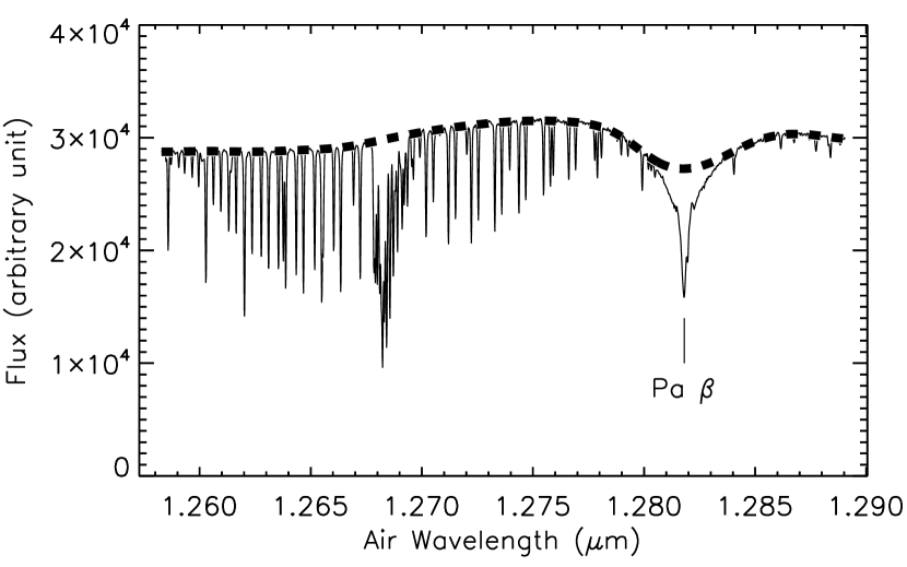
Figure 1: Continuum normalization of an A0 V star (order 44). The solid line indicates the observed spectrum, while the dashed line indicates the fitted continuum spectrum determined using the IRAF task continuum. Note that the majority of the absorption lines seen in this figure are from telluric absorption (mainly caused by O₂ molecules in this wavelength region). As discussed in the text, the continuum obtained here is not suitable for studying the Pa $\beta$ line but works sufficiently for our purpose of using this spectrum for telluric correction.

Although the continuum task skillfully estimates the continua of observed spectra for most orders, it often fails at around 9,300–9,600 Å, where telluric absorption is very severe. In such cases, the observed spectrum is first processed using molecfit for rough removal of telluric absorption lines and the continuum task is then performed to estimate the continuum level. This additional procedure often improves the results of the continuum-normalized spectrum.

3.2 Making synthetic telluric spectra

The next step is to use molecfit to create a synthetic telluric spectrum $[T(\lambda;A_{\mathrm{std}})*P(\lambda)]_{\mathrm{model}}$ using the normalized spectrum of the telluric standard star. It should be noted that in our method the created synthetic spectrum is used only as a reference for identifying spectral features other than telluric absorption on the spectrum of a telluric standard star. At this step, it is unnecessary to fine-tune the molecfit parameters to remove the telluric lines perfectly, but finding a reasonably good solution is useful in making the following steps simple and efficient. Some key points regarding tuning the settings of molecfit to achieve such accuracy are described below, but readers are also referred to Smette et al. (2015) and to the molecfit manual for more details on its functions.

We run molecfit for each spectral order independently to create synthetic telluric spectra. The instrumental profile $P(\lambda)$ is determined through a fitting in which $P(\lambda)$ is modeled as a combination of Gaussian and Lorentzian curves. Only the molecules listed in the last column in Table 1 are included in the calculation and fitted for each spectral order, and the other molecules are switched off because they have negligible contribution on results. We have found that the initial value of the H₂O scaling factor often has significant impacts on the fit, and a careful tuning of this parameter is one of the most important factors in achieving high accuracy. In addition, masking spectral features other than telluric absorption is also important. The wavelength ranges holding the intrinsic A0 V star absorption lines as predicted by a model spectrum, created by using SPTOOL (Takeda, private communication) to implement ATLAS9 programs (Kurucz 1993), are masked. Other spectral features including artifacts are also checked by eye and masked if necessary.

An example of a synthetic telluric spectrum $[T(\lambda;A_{\mathrm{std}})*P(\lambda)]_{\mathrm{model}}$ created by molecfit for a specific spectral order is shown in Figure 2. From this figure, we observe that the difference between observation and model, or $\Delta(\lambda)$, has uncertainties at a few percent level, which is rather large in comparison to the uncertainties obtained by classical methods using telluric standard spectra. This result is likely caused by poor accuracy of modeling of the instrumental profile $P(\lambda)$ and the slight wavelength uncertainties of the WINERED spectra. Further fine tuning of molecfit parameters can improve these results, although noisy features of a few percent were persistent during our analysis. As mentioned above, the purpose of using molecfit at this step is not to completely remove the telluric lines by itself.

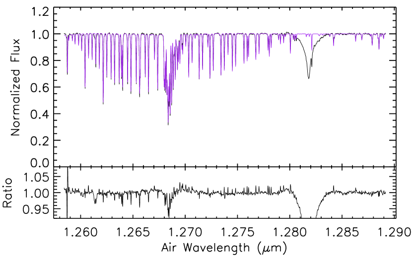
Figure 2: Top: Comparison between a synthetic telluric spectrum created using molecfit and an observed spectrum. The black line indicates the normalized telluric standard spectrum $O^{\prime}_{\mathrm{std}}(\lambda)$, while the purple line indicates the synthetic telluric spectrum $[T(\lambda;A_{\mathrm{std}})*P(\lambda)]_{\mathrm{model}}$. Bottom: $R(\lambda)$, the ratio of the observed spectrum to the synthetic telluric spectrum.

3.3 Fitting intrinsic stellar lines

Intrinsic stellar lines of an A0 V star present in the ratio spectrum $R(\lambda)$ are manually fitted and subsequently removed by visual inspection with the help of an A0 V star model spectrum created by SPTOOL. Multiple Gaussian curves are used as a fitting function, and fittings are performed by minimizing chi-squared values using the IDL script mpfit.pro (Markwardt 2009), which uses the Levenberg-Marquardt method. It should be noted that, in addition to intrinsic stellar lines, features other than telluric absorption such as residuals of sky subtraction and flat-fielding-related incompleteness appear in the ratio spectrum. These are carefully removed at this stage by fitting multiple Gaussian curves. Generally speaking, identification and fitting are relatively easy for narrow and deep absorption lines; for this reason, A0 V stars with $v\sin i\lesssim 50$ km s^-1 are generally selected as telluric standard stars in the proposed method.

An example of fitting of the intrinsic stellar lines of an A0 V star is shown in Figure 3. In this case, the Pa $\beta$ profile is asymmetric owing to an error in the continuum normalization. Such spectra are unsuitable for studying the Pa $\beta$ line itself, but a (skewed) profile could be reproduced by combining three Gaussian curves. Moreover, we could also identify two weak metal lines—C I $\lambda\lambda 12601,12614$—in this spectral order. Although these weak lines were somewhat blended with the noisy features due to the imperfect matching of synthetic telluric spectra in the previous step, we could fit a single Gaussian curve by masking a couple of pixels showing significant deviations. By contrast, C I $\lambda 12679$ could not be fitted because it appeared to be very weak and seriously blended with deep telluric absorption. Over the entire wavelength range of WINERED, i.e., from 0.90–1.35 µm, we identified more than 100 metal lines, with depths as shallow as $\sim$1%. This result directly suggests the importance of removing intrinsic stellar lines in NIR high-resolution spectroscopy, even if a featureless A-type star is used as a telluric standard star.

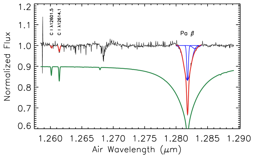
Figure 3: Schematic illustrating how the intrinsic stellar lines of an A0 V star are identified and fitted. The black line indicates the ratio spectrum $R(\lambda)$, i.e., the observed spectrum of a telluric standard star divided by a synthetic telluric spectrum. The green line indicates the model spectrum of an A0 V star created using SPTOOL and shifted in vertical direction for visual clarity. The fitted intrinsic stellar lines, indicated by the red curves, are obtained by combining up to three Gaussian functions, each of which is indicated by a blue curve.

4 Results

Table 2: Observing Log

Name	Spectral Type	UT Date	UT Start	Airmass	Seeing	$T_{\mathrm{air}}$	RH	Exposure	SNR
					(arcsec)	(∘C)	(%)	(sec)
HD 2905	B1 Ia	2014 Jan 22	09:55:26	1.24–1.27	4.3	$+0.9$	78	720	830
HD 23180	B1 III	2014 Jan 22	12:20:48	1.08–1.08	4.0	$-0.1$	84	400	600
7 Cam	A1 V	2014 Jan 22	12:35:16	1.07–1.08	3.8	$-0.2$	84	960	750
HD 30614	O9 Ia	2014 Jan 22	13:02:26	1.19–1.21	3.4	$-0.2$	85	960	810
HD 37022	O7 V	2014 Jan 22	13:34:36	1.38–1.42	3.5	$+0.2$	84	960	700
HD 25204	B4 IV	2014 Jan 23	10:57:21	1.08–1.09	3.9	$+1.6$	82	720	1040
HD 36371	B4 Ib	2014 Jan 23	11:18:31	1.03–1.02	3.9	$+1.3$	83	720	800
HD 36822	B0 III	2014 Jan 23	12:15:43	1.11–1.11	4.0	$+0.8$	85	1200	740
HD 37742	O9.2 Ib	2014 Jan 23	12:46:56	1.26–1.26	4.4	$+0.3$	86	240	1160
HD 37043	O9 III	2014 Jan 23	13:08:07	1.35–1.40	4.1	$+0.4$	85	600	890
HD 41117	B2 Ia	2014 Jan 23	13:49:34	1.06–1.07	3.7	$+0.2$	85	720	760
HD 36486	B0 III + O9 V	2014 Jan 23	14:08:37	1.38–1.40	3.9	$+0.1$	85	240	810
HD 43384	B3 Iab	2014 Jan 23	14:26:38	1.07–1.10	3.7	$+0.0$	86	1440	580
21 Lyn	A0.5 V	2014 Jan 23	15:00:30	1.04–1.06	3.5	$-0.1$	85	1200	830
$\varepsilon$ Leo	G1 IIIa	2014 Jan 23	16:44:32	1.02–1.03	3.3	$-0.8$	85	110	1010

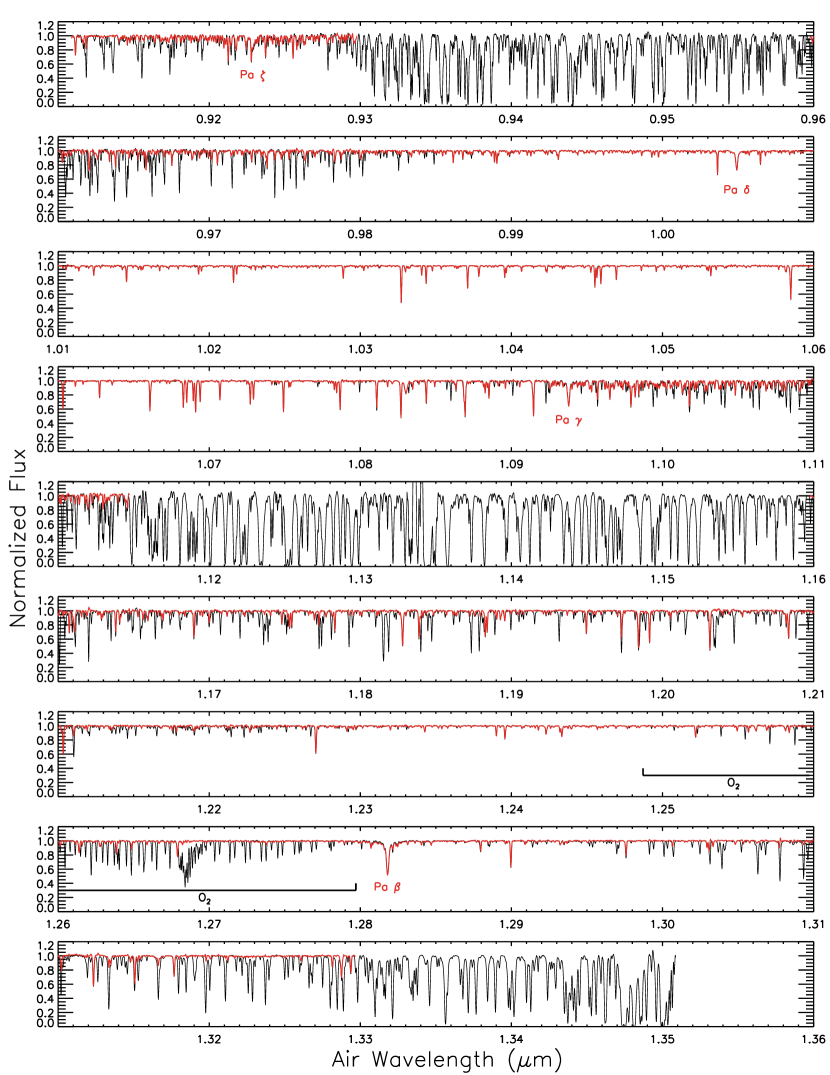
Figure 4: WINERED spectrum of $\varepsilon$ Leo (G1 IIIa) before (black) and after (red) telluric correction. The wavelength ranges 0.930–0.960, 1.115–1.160, and $>$1.330 µm, are not treated with telluric correction owing to the heavy telluric absorption in these ranges.

Here, we show some examples of applying the method described in §§2–3 to spectra obtained using WINERED. The observing log of all target objects and telluric standard stars is summarized in Table 2. In the following analysis, 7 Cam (A1 V) and 21 Lyn (A0.5 V) were used as telluric standard stars for target objects observed on Jan 22 and 23, 2014, respectively. For these observations, WINERED was attached to the 1.3-m Araki telescope at the Koyama Astronomical Observatory. The air temperature outside the dome changed from $+1.5$ to $-1^{\circ}$C and the relative humidity changed from $76$ to $86$% during the nights, which are typical conditions of the winter season of the site. Seeing ranged from 3″.3 to 4″.4, which were slightly worse than the typical value of the site ($\sim$3″.0).

Figure 4 compares the spectra before and after telluric correction obtained from the G1 III giant $\varepsilon$ Leo over the entire wavelength range covered by WINERED. Because telluric absorption was too heavy in the wavelength ranges 0.930–0.960, 1.115–1.160, and $>$1.330 µm, which correspond to the gaps between the adjacent photometric bands ($z^{\prime},Y$ and $J$), we did not perform any telluric correction for these ranges. Apart from these extreme regions, our method effectively removed telluric absorption lines even in, e.g., the strong O₂ band (1.25–1.28 µm) and successfully reproduced the intrinsic spectrum of $\varepsilon$ Leo.

Figure 5 plots the spectrum of $\varepsilon$ Leo in the 61st order before and after telluric correction along with the telluric absorption spectrum. In the original spectrum, stellar lines are heavily contaminated by telluric absorption lines, which prevented quantitative investigations of intrinsic features. By contrast, the spectrum obtained after telluric correction is in close agreement with the model stellar spectrum created by SPTOOL, demonstrating the applicability of our method to even feature-rich objects. The sophisticated telluric correction we obtained enabled us to identify a large number of weak metal and CN molecular lines for $\varepsilon$ Leo, which we will compile as a line list and report in a forthcoming paper (Ikeda et al., in preparation).

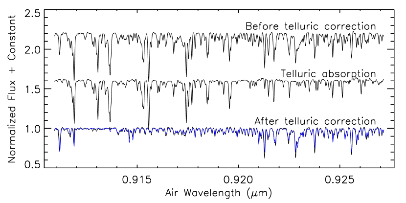
Figure 5: Telluric correction of $\varepsilon$ Leo (G1 IIIa) for spectral order 61. The spectra are shown from top to bottom as follows: the raw spectrum of $\varepsilon$ Leo, the telluric absorption spectrum $S(\lambda;A_{\mathrm{tgt}})$ created from 21 Lyn (A0.5 V), and the telluric-corrected spectrum of $\varepsilon$ Leo. A model spectrum of $\varepsilon$ Leo created by SPTOOL is indicated in blue. For visual clarity, constants are added to the top and middle spectra.

As another example, the results of telluric correction for several OB stars are illustrated in Figure 6. In the observed wavelength range 1.09–1.11 µm, serious absorption by water vapor makes it difficult to properly trace stellar features such as Pa $\gamma$. Our method successfully removed the telluric absorption for all objects, making it possible to trace the entire line profiles of several lines, including Pa $\gamma$. Moreover, the weak helium lines—He I $\lambda\lambda 10996.6,11013.1,11045.0$—are barely identifiable in the observed spectra but are clearly identified for some objects after telluric correction.

Figure 6: Spectra (order 51) of 12 OB stars prior to (left panel) and after telluric correction (right panel). Each spectrum is shifted so that the line center of Pa $\gamma$ lies at 10938.09 Å. Note that the spike feature near Pa $\gamma$ in HD 37022 is not caused by error in the telluric correction but due to incomplete subtraction of the emission line from the surrounding Orion Nebula.

5 Discussion

The aim of this study was to establish a method for correcting telluric absorption in NIR high-resolution and high-SNR spectra. The proposed method uses A0 V stars or their analogs as telluric standard stars whose intrinsic stellar lines were carefully removed with the help of synthetic telluric spectra created using molecfit as a reference. As presented in the previous section, our method works effectively even for feature-rich G-type stars and can successfully reproduce weak stellar lines that are barely identifiable in the observed spectrum prior to removal of heavy telluric absorption.

In the following subsections, we will evaluate the accuracy of our method by comparing it to other methods and through the use of a newly developed diagnostic method. We will also investigate the dependence of telluric correction on observing conditions, i.e., airmass and time, in a quantitative manner.

5.1 Comparison with simple spectral division by early-type stars

Figure 7: Comparison between observed and corrected spectra of $\varepsilon$ Leo (order 44) with three different telluric corrections considered: ($b$) division by an A0.5 V star (21 Lyn), ($c$) division by an O9.2 Ib star (HD 37742), and ($d$) our method.

An observed spectrum of a featureless early-type star is sometimes used to correct telluric absorption without removal of its stellar lines. Here, we demonstrate some of the limitations of this approach relative to our method. Figure 7 shows the observed spectrum of $\varepsilon$ Leo for spectral order 44 divided by that of an A- or O-type star and a spectrum corrected using our method. The performance of the respective approaches are summarized as follows:

1. Spectral division by an A-type star significantly distorts the Pa $\beta$ line. Furthermore, two emission-like residuals are seen at $\sim$12,603 Å and $\sim$12,615 Å as a result of C I $\lambda\lambda 12601,12614$ absorption lines of the A-type star, respectively (see Figure 3). It is seen that, in the case of NIR high-resolution and high-SNR spectra, both the strong hydrogen and weak metal lines of a telluric standard star should be removed. From our analysis of WINERED spectra we found that even A0 V stars have $\sim$100 metal lines that must be removed at 0.90–1.35 µm. The strengths of these metal lines vary considerably with $v\sin i$, metallicity, chemical composition, etc., which prevented us from transforming the spectrum of Vega into that of another A-type star by changing the scales and widths of the stellar lines, as required in the method proposed by Vacca et al. (2003).

2. O-type stars might serve as better telluric standards than A-type stars because they have smaller numbers of metal lines. Moreover, their high rotational velocities make their absorption lines shallow, resulting in weak residuals in the target spectrum after telluric correction. However, O-type stars have many strong hydrogen and helium lines that must be fitted and removed. This is clearly illustrated in Figure 7($c$), in which there are bumps at $\sim$1.279 and $\sim$1.282 µm corresponding to He I $\lambda\lambda$12784, 12790 and Pa $\beta$, respectively, in the O-type star. Other problems in using O-type stars as telluric standards include: (1) their sparse distribution on the celestial sphere compared to A-type stars, and; (2) the fact that they often have strong emission lines from surrounding gas.

3. Unlike simple spectral division with A- and O-type stars, our method does not disturb the spectral components around Pa $\beta$. In addition, it does not have to account for emission-line-like noises owing to the weak metal lines found in telluric standard stars. Our method is therefore quite effective in correcting the telluric absorption in NIR high-resolution and high-SNR spectra. However, our method does have some disadvantages. It requires somewhat tedious procedures involving the manual fitting of many weak metal lines and some strong hydrogen lines. One possible way to significantly reduce this burden is to reapply the fitted intrinsic spectrum $[I_{\mathrm{std}}^{\prime}(\lambda)*P(\lambda)]_{\mathrm{fit}}$ to the observed spectra of the same standard star taken at different times. By routinely observing selected A0 V stars in this manner, it would be possible to automatically remove their intrinsic stellar lines. After several experiments along these lines, we found that a satisfactory level of removal can be achieved for weak metal lines, but non-negligible residuals remain around the hydrogen lines, primarily because of the uncertainty in continuum normalization around such broad lines; further investigations will be required along these lines.

5.2 Quality of telluric correction

We also developed a new diagnostic method for evaluating the quality of telluric correction. Here, we denote the fluxes of a continuum-normalized spectrum before and after telluric correction as $F(\lambda)$ and $G(\lambda)$, respectively. If the correction is perfect, $G(\lambda)$ should be unity at positions where the intrinsic stellar lines of the target are not present. The deviation of $G(\lambda)$ from unity can be used, in addition to the dispersion of $G(\lambda)$, as a quality indicator of telluric correction. Furthermore, unless the accuracy of the performed telluric correction is poor the ratio $F(\lambda)/G(\lambda)$ can be regarded as an approximation of the atmospheric transmittance $T(\lambda)$. Therefore, by comparing $G(\lambda)$ and $F(\lambda)/G(\lambda)$, we can quantitatively examine the accuracy of telluric correction and its dependence on atmospheric transmittance.

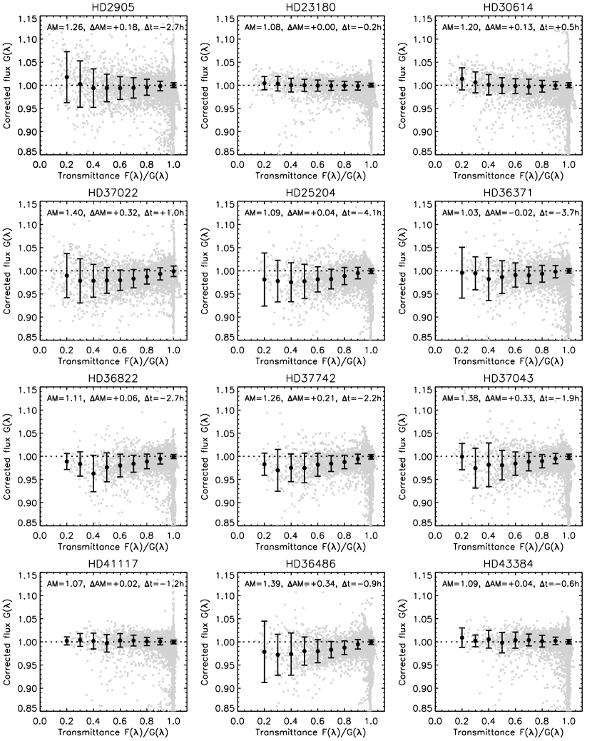
Figure 8: Quality-diagnostic diagrams for 12 OB stars. Gray dots indicate the telluric-corrected flux $G(\lambda)$ plotted against $F(\lambda)/G(\lambda)$, a proxy for atmospheric transmittance, for each pixel outside of the O₂-band region (1.245–1.280 µm). The circles and error bars indicate, respectively, the sigma-clipped mean and standard deviation for each transmittance bin ($\Delta=0.1$). The mean airmass of the target, the difference in airmass from that of the telluric standard star, and the time difference are given in each panel.

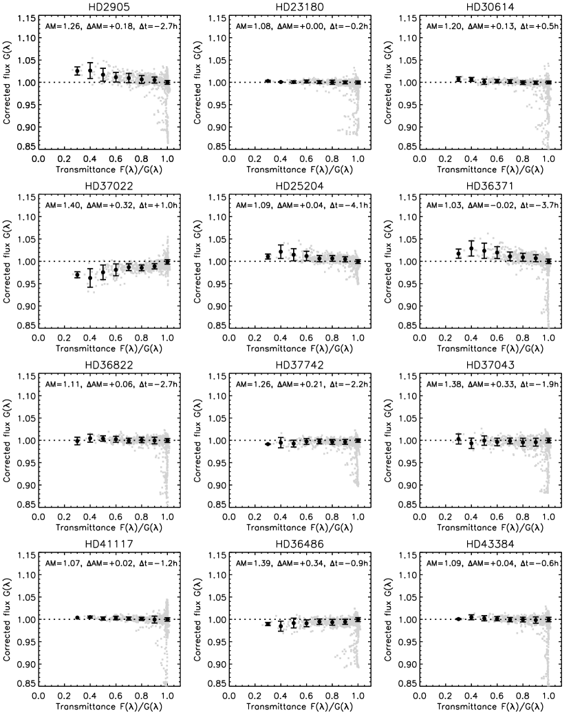
Figure 9: Quality-diagnostic diagrams for 12 OB stars as Figure 8, but using data in the O₂-band region (1.245–1.280 µm).

We applied the above diagnostic method to the 12 OB stars listed in Table 2. To check differences among the absorbers, we separated the star’s spectral parts into two groups that are either affected primarily by water vapor absorption or by molecular oxygen absorption; the results are illustrated in Figures 8 and 9, respectively. Note that the wavelength ranges 0.930–0.960, 1.115–1.160, and $>$1.330 µm were not included in our analysis (see §4). Because intrinsic stellar lines also lead to offsets of $G(\lambda)$ from unity, this diagnostic works better for featureless objects; for this reason, we excluded $\varepsilon$ Leo from this analysis. The scattering seen in Figures 8 and 9 is caused by various factors including random noise owing to SNR, systematic deviations owing to intrinsic stellar lines, and inaccuracies in continuum normalization. Note that, in our case, the SNR is high enough and the especially large vertical scatter seen at $F(\lambda)/G(\lambda)\sim 1$ mainly reflects the intrinsic stellar lines of the target. In addition, stellar features are expected to give outliers at each level of $F(\lambda)/G(\lambda)$ smaller than one. To avoid such stellar contamination, we calculated 3-sigma-clipped means and standard deviations for each bin of $F(\lambda)/G(\lambda)$, which are plotted in the figure.

It is seen from Figure 8 that the quality of telluric correction is particularly good for HD 23180, HD 41117, and HD 43384. In these cases, the deviation of $G(\lambda)$ from unity is $\lesssim 1$% and the dispersion of $G(\lambda)$ is $\lesssim 2$%, even at $F(\lambda)/G(\lambda)\sim 0.2$; this indicates that our method works for atmospheric transmittances as low as $\sim$20%. In all these cases, (1) the airmass differs from that associated with the telluric standard star by $\lesssim 0.05$, and (2) the time differs by $\lesssim 1$ h. In other words, telluric standard stars should be observed to fulfill these criteria at the Koyama Astronomical Observatory. Considering high humidity ($\gtrsim$80%) and relatively unstable weather conditions at the Koyama Astronomical Observatory, it may safely be said that these criteria would be relaxed at sites with better conditions like Paranal or Mauna Kea.

As seen in Figure 9, the dispersion of $G(\lambda)$ for molecular oxygen absorption is generally small compared to that for water vapor absorption. However, in some cases offsets from unity are seen in $G(\lambda)$ where the telluric transmittance is low. We determined that these offsets are primarily caused by the absorption at 1.268–1.270 µm, where telluric lines are closely blended with each other. This may indicate that changes in line shape as a function of airmass and time are different for isolated telluric and blended lines; thus, simple scaling of the standard spectrum optimized for unblended telluric lines results in offsets of $G(\lambda)$ from unity for blended lines. It is remarkable that, even in such extreme regions, telluric correction can be performed successfully based on observations fulfilling the above conditions on airmass and time.

We also applied our diagnostic method to the G-type giant $\varepsilon$ Leo and obtained the result shown in Figure 10. Because $\varepsilon$ Leo has many intrinsic absorption lines, it produces a non-negligible number of $G(\lambda)$ that deviate from unity even under perfect telluric correction. Therefore, we plotted $G(\lambda)/G_{\mathrm{model}}(\lambda)$ on the vertical axis instead of $G(\lambda)$, where $G_{\mathrm{model}}(\lambda)$ is a model spectrum of $\varepsilon$ Leo created by SPTOOL (see §4). As seen in the figure, the difference between the corrected and model spectra as measured by the standard deviation of $G(\lambda)/G_{\mathrm{model}}(\lambda)$ is less than 5% at $0.2\lesssim F(\lambda)/G(\lambda)\lesssim 1$. The scatter is larger than the best cases in Figure 8 but similar to those cases with relatively large scatters. Note that, as the scatter in Figure 10 includes errors in the model spectrum, the scatter is an upper limit of the accuracy of the telluric correction applied to $\varepsilon$ Leo. In fact, the standard deviation in Figure 10 is larger at $F(\lambda)/G(\lambda)=1$ than those in Figures 8 and 9 and increases slowly with decreasing $F(\lambda)/G(\lambda)$, which indicates the significant contribution of error sources other than the telluric correction. This confirms that our method can produce telluric corrections with an accuracy of 5% or better for G-type stars.

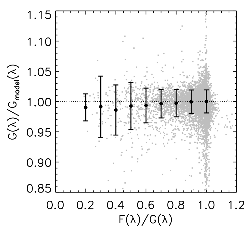
Figure 10: Quality-diagnostic diagram for $\varepsilon$ Leo presented in the same manner as in Figure 8 but using $G(\lambda)/G_{\mathrm{model}}(\lambda)$ as the vertical axis instead of $G(\lambda)$.

5.3 Comparison with molecfit

Comparing our method with molecfit should be useful for readers to select their strategies for observation because very accurate telluric correction may not be needed for many scientific cases, for which observing telluric standard stars may be expensive in terms of telescope time. For medium-resolution spectra, Kausch et al. (2015) compare a classical method based on telluric standard stars and the telluric correction by molecfit using VLT/X-Shooter spectra. Here, we compare the two methods for NIR high-resolution spectra by using WINERED spectra ($R\sim 28,000$).

We used the spectra of HD 23180 (B1 III; see Table 2) for the test. To optimize the molecfit parameters, we first obtained best-fit parameters from the fitting of the telluric standard star (7 Cam) following the procedures written in §3.2 and put them as initial values in the fitting of HD 23180. Because the intrinsic stellar lines of HD 23180 are strong and wide, they could be distinguished from telluric absorption lines and masked to improve the fitting.

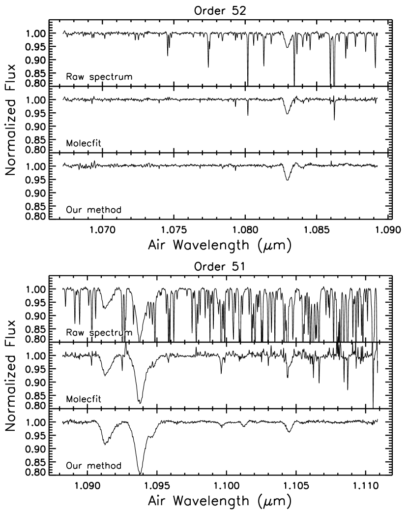
Figure 11: Telluric correction of HD 23180 by our method and molecfit for the orders 52 (upper panel) and 51 (lower panel). In each panel, the raw spectrum, which is not corrected for telluric absorption, is shown for reference.

In Figure 11, the resultant telluric correction of HD 23180 by molecfit is compared to that with our method for the orders 52 and 51. Molecfit can nicely correct telluric absorption overall, but the fitting residual becomes non-negligible at the wavelength region where absorption lines are strong and blended. Although we tried fine-tuning parameters as much as possible, those fitting residuals could not be removed. This must be partly due to imperfect modeling of the instrumental profile and wavelength solution in our molecfit running, but there may be another possibility. Those strong absorption lines may be saturated in reality but residual flux shows up in their core owing to instrumental smearing. If that is the case, Figure 11 may imply that our method can correct even for moderately saturated telluric lines with an accuracy of the order of 2% or better of the continuum , while Smette et al. (2015) report that molecfit can reach such an accuracy in correcting unsaturated lines.

The diagnostic method introduced in §5.2 can be applied to spectra corrected by molecfit, which enables a direct comparison between the two methods in a quantitative manner. Figure 12 shows the result for the molecfit-corrected spectrum of HD 23180. Telluric correction with molecfit results in larger scattering than our method (see Figure 8) and the deviation of the corrected flux $G(\lambda)$ from unity increases as the transmittance decreases; $G(\lambda)$ becomes noticeably low ($<0.95$) at the transmittance $F(\lambda)/G(\lambda)<0.5$. This quantitative analysis is consistent with the qualitative analysis above (see Figure 11). Similar trends are also found for all OB stars, for which we tried the same test. As discussed above, the deviation of $G(\lambda)$ from unity at low transmittance may be due to saturated absorption lines, while molecfit works fine for unsaturated absorption lines.

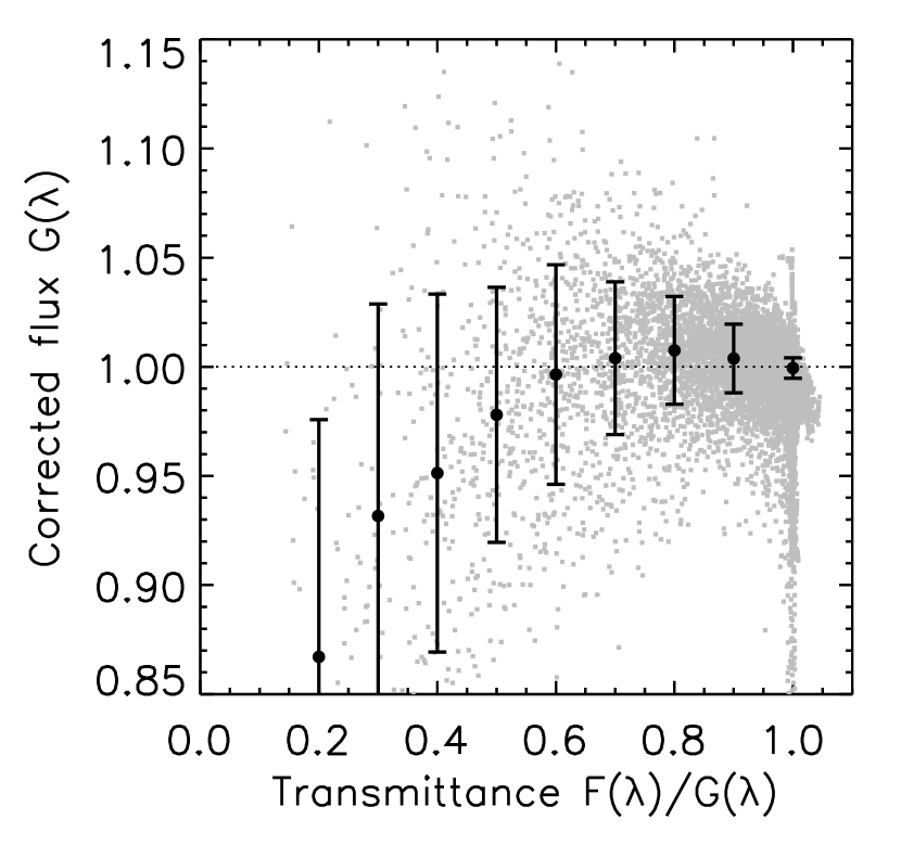
Figure 12: Quality-diagnostic diagram of HD 23180 whose telluric absorption is corrected by molecfit. Pixels outside of the O₂-band region (1.245–1.280 µm) are used in the plot as in Figure 8.

Another interesting test is to use the best-fit transmission curve created by molecfit from a science target spectrum as a pseudo-target spectrum and apply our method to it. In the ideal case, this will produce a straight line at unity. Deviations from unity will arise from any one of the following: incompleteness in the molecfit modeling, inaccuracies in our method, and noise. The spectrum of HD 23180 (order 51) was used for this test and the result is shown in Figure 13. As can be seen from the lower panel in the figure, the deviations of $\gtrsim 1$% are mainly seen where telluric absorption is strong, indicating differences between the two methods at those regions. Significant deviations are not confirmed at the wavelength region where intrinsic lines of a telluric standard star were removed. In addition to such high-frequency deviations, low-frequency deviations with an amplitude of $<1$% are also confirmed in the spectrum. This is due to the inaccuracies in the continuum normalization of a telluric standard star’s spectrum, which is almost inevitable at the wavelength region where telluric absorption lines are crowded. As Kausch et al. (2015) pointed out, inaccuracies in continuum normalization is one of the disadvantages of classical methods using telluric standard star. Although it is beyond the scope of this paper, extracting low-frequency function from this spectrum and use it to improve the continuum normalization of the telluric standard star could be a good idea to overcome the normalization problem.

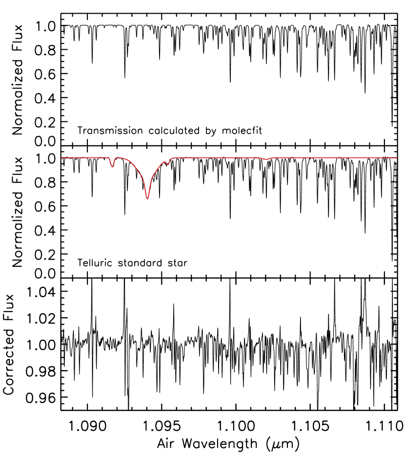
Figure 13: Upper panel: best-fit transmission curve created by molecfit from HD 23180 (order 51). Middle panel: spectrum of the telluric standard star 7 Cam (black) and the removed intrinsic stellar lines (red). Lower panel: after the telluric correction of the best-fit transmission curve (upper panel) using the telluric standard star spectrum (middle panel) by our method.

To summarize, molecfit effectively corrects unsaturated telluric lines with the accuracy which many science cases require. On the other hand, the above tests indicate that our method is applicable even to strong telluric lines with moderate saturation. If the target line is very faint ($\lesssim$ a few % in depth) and blended with strong telluric lines (see, e.g., C I lines at $\sim$1.26 µm in Figure 3; He I lines at $\sim$1.10 µm in Figure 6), our method could be an efficient way to correct telluric absorption.

5.4 Effects of separations in airmass and time

Table 3: Observing Conditions

Name	Standard	Difference from Standard		$\sigma_{50}$
		Airmass	Time (hour)	H2O	O2
HD 2905	7 Cam	$+0.18$	$-2.7$	0.0298	0.0107
HD 23180	7 Cam	$+0.00$	$-0.2$	0.0131	0.0033
HD 30614	7 Cam	$+0.13$	$+0.5$	0.0170	0.0039
HD 37022	7 Cam	$+0.32$	$+1.0$	0.0278	0.0132
HD 25204	21 Lyn	$+0.04$	$-4.1$	0.0368	0.0105
HD 36371	21 Lyn	$-0.02$	$-3.7$	0.0353	0.0132
HD 36822	21 Lyn	$+0.06$	$-2.7$	0.0313	0.0067
HD 37742	21 Lyn	$+0.21$	$-2.2$	0.0319	0.0065
HD 37043	21 Lyn	$+0.33$	$-1.9$	0.0318	0.0085
HD 41117	21 Lyn	$+0.02$	$-1.2$	0.0188	0.0040
HD 36486	21 Lyn	$+0.34$	$-0.9$	0.0304	0.0076
HD 43384	21 Lyn	$+0.04$	$-0.6$	0.0221	0.0048
$\varepsilon$ Leo	21 Lyn	$-0.03$	$+1.7$	0.0391	0.0091

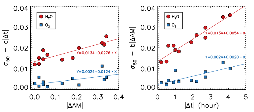
Figure 14: $\sigma_{50}$; standard deviations of the corrected flux at an atmospheric transmittance of 50% (see text for further details) plotted against the difference in airmass (left) and time (right). In both panels, the contribution of other parameters to $\sigma_{50}$ are removed using Eq. (8). The red circles and blue boxes indicate, respectively, the results for absorption by water vapor and molecular oxygen. The results of multiple linear regression are indicated with solid lines.

Here, we discuss in more detail how observing conditions, i.e., differences in airmass and time between a target and a standard star, affect the accuracy of telluric correction. We use $\sigma_{50}$ to denote the standard deviation of $G(\lambda)$ at $0.45<F(\lambda)/G(\lambda)<0.55$, which indicates the accuracy of the correction for pixels for which telluric absorption is as deep as 50%. The $\sigma_{50}$ values measured for the 12 OB stars and $\varepsilon$ Leo are listed in Table 3, along with the differences in airmass and time from those associated with the standard stars. Using the data for the 12 OB stars, we performed multiple linear regression assuming the following model:

$$\sigma_{50}=a+b\,|\Delta\mathrm{AM}|+c\,|\Delta t|,$$ (8)

where $|\Delta\mathrm{AM}|$ and $|\Delta t|$ are the absolute values of the difference in airmass and time in hours, respectively. Least-squares fitting produces the coefficients $(a,b,c)=(0.0134,0.0276,0.0054)$ for water vapor absorption and $(0.0024,0.0124,0.0020)$ for molecular oxygen absorption. This indicates that, even in the case of water vapor absorption, $\sigma_{50}\lesssim 2\%$ can be maintained if $|\Delta\mathrm{AM}|\lesssim 0.05$ and $|\Delta t|\lesssim 1$ h, which is consistent with the discussion in the previous subsection. In Figure 14, $\sigma_{50}-c\,|\Delta t|$ and $\sigma_{50}-b\,|\Delta\mathrm{AM}|$ are plotted against $|\Delta\mathrm{AM}|$ and $|\Delta t|$, respectively, to clarify the dependence of $\sigma_{50}$ on each parameter separately.

We also performed partial correlation analysis to remove interdependence among the parameters. The partial correlation coefficients between $\sigma_{50}$ and $|\Delta\mathrm{AM}|$ were calculated using the IDL procedure p_correlate.pro as follows:

$$r(\sigma_{50,\mathrm{H_{2}O}},|\Delta\mathrm{AM}|;|\Delta t|) = 0.849\ (<4.8\times 10^{-4}),$$ (9)

$$r(\sigma_{50,\mathrm{O_{2}}},|\Delta\mathrm{AM}|;|\Delta t|) = 0.591\ (<0.043),$$ (10)

where $r(X,Y;Z)$ denotes the partial correlation coefficient between $X$ and $Y$ holding $Z$ fixed, $\sigma_{50,\mathrm{H_{2}O}}$ and $\sigma_{50,\mathrm{O_{2}}}$ are the $\sigma_{50}$ for water vapor and molecular oxygen absorption, respectively, and the parenthesis in the right-hand side indicates the $p$-value. Thus, at a significance level of 0.05 both $\sigma_{50,\mathrm{H_{2}O}}$ and $\sigma_{50,\mathrm{O_{2}}}$ positively correlate with $|\Delta\mathrm{AM}|$. This result leads to the naturally expected conclusion that the accuracy of telluric correction improves when the airmass difference between the target and telluric standard is reduced. Note, however, that this holds even if a correction for airmass difference based on Beer’s law is performed, as is done in our method. Next, the partial correlation coefficients between $\sigma_{50}$ and $|\Delta t|$ were calculated as

$$r(\sigma_{50,\mathrm{H_{2}O}},|\Delta t|;|\Delta\mathrm{AM}|) = 0.951\ (<2.0\times 10^{-6}),$$ (11)

$$r(\sigma_{50,\mathrm{O_{2}}},|\Delta t|;|\Delta\mathrm{AM}|) = 0.751\ (<4.9\times 10^{-3}).$$ (12)

Although positive correlation is confirmed at a significance level of $5\times 10^{-3}$ in both cases, the correlation coefficient is obviously larger for water vapor than for molecular oxygen. This is probably because the column density of water vapor along a given line of sight is much more sensitive to temperature and variable over time than the column density of molecular oxygen. Besides, the azimuthal dependence of water vapor concentration may be attributed to the larger correlation coefficient while molecular oxygen is expected to be almost constant. Our result suggests that, at least at the Koyama Astronomical Observatory, where the weather condition can change fairly rapidly, the time and azimuthal variation of the telluric absorption lines cannot be fully adjusted by simply changing the variable $\beta$ in Eq. (6). Thus, in NIR spectroscopic observation it is of great importance to observe a telluric standard star before or after observing the target object in either case, preferably within one hour.

6 Summary

We developed a telluric correction method for NIR high-resolution spectra observed using the WINERED spectrograph. The proposed method uses an A0 V star or its analog as a telluric standard star. Because careful removal of intrinsic stellar lines of the telluric standard star is crucial in the case of high-resolution and high-quality spectra, we developed a manual process for doing so involving the use of a synthetic telluric spectrum created using molecfit. By removing the many weak metal lines identified in the spectrum of an A0 V star, our method can successfully correct telluric absorption without disturbing the intrinsic spectral features of targets including feature-rich G-type stars.

We further developed a new diagnostic method to evaluate the accuracy of telluric correction. From the application of this diagnostic to 12 OB stars whose spectra were obtained using WINERED at the Koyama Astronomical Observatory, we found that we could obtain telluric correction for spectral parts for which the atmospheric transmittance is as low as 20% with accuracies better than 2% if the following conditions are fulfilled: (1) the difference in airmass between the target and the telluric standard star is $\lesssim 0.05$, and; (2) that in time is $\lesssim 1$ h. Although readers should take care that the result is based on a low number statistics and heavily dependent on the observing site, it would be used as a guide at other sites. Given that the humidity tends to be high at the Koyama Astronomical Observatory ($\sim$80% on the two nights discussed in this paper), the above conditions may be relaxed for other observation sites with better weather conditions. We also applied our diagnostic method to the G-type giant $\varepsilon$ Leo and found that the reproduced spectrum matched a model spectrum with better than 5% accuracy. Comparison with the telluric correction by molecfit implies that our method may be applicable to strong telluric absorption lines which are moderately saturated. The accuracy of telluric correction depends on both the difference in airmass and time, with the latter appearing to have a particularly large impact for water vapor absorption, probably because the time variability of water vapor and the corresponding spectral change cannot be fully reproduced by simply scaling a reference spectrum. Consequently, minimizing the difference in time between the target and the telluric standard star is of particular importance in NIR spectroscopic observation.

$$O^{\prime}(\lambda)=[I^{\prime}(\lambda)\cdot T(\lambda)]*P(\lambda),$$ (1)

where $I(\lambda)$ is the intrinsic spectrum of the target star, $T(\lambda)$ is the telluric absorption spectrum, $P(\lambda)$ is the instrumental profile, and the asterisk and prime symbol denote convolution and continuum normalization, respectively. In spectral analysis, this equation is often regarded as

$$O^{\prime}(\lambda)\sim[I^{\prime}(\lambda)*P(\lambda)]\cdot[T(\lambda)*P(\lambda)].$$ (2)

Then, dividing $O^{\prime}(\lambda)$ by the factor $[T(\lambda)*P(\lambda)]$ derived from either the spectrum of the telluric standard star or a synthetic telluric spectrum, we can extract the (instrumentally smeared) target spectrum $[I^{\prime}(\lambda)*P(\lambda)]$. This procedure is usually considered to be the “telluric correction.” However, the above two equations differ mathematically, and the difference between $[I^{\prime}(\lambda)*P(\lambda)]$ and $O^{\prime}(\lambda)/[T(\lambda)*P(\lambda)]$ cannot be neglected in some cases. Here, we discuss this problem in a quantitative manner using simple simulations.

The settings for our simulation are summarized as follows. We created a synthetic telluric spectrum $T(\lambda)$, using the radiative transfer code LBLRTM (Clough et al. 2005). The spectral resolution of $T(\lambda)$ was set to be very high ($R\sim 500,000$) to enable simulation of intrinsic telluric absorption with avoiding instrumental smearing effects. A Gaussian curve of width corresponding to the spectral resolution of WINERED ($R\sim 28,000$) was adopted as the instrumental profile $P(\lambda)$, and convolution was performed using the IDL script gaussfold.pro. Starting out with artificial absorption lines with Gaussian profiles that were isolated in the stellar spectrum $I^{\prime}(\lambda)$ but blended with telluric absorption lines, we then simulated several cases by varying the width of the Gaussian profile and the degree of blending.

An example of this simulation is shown in Figure 15, in which two artificial stellar lines are located at around 12005.0 and 12008.5 Å, respectively; the former is blended with the telluric line at 12004.7 Å but separated by about the width of the instrumental profile, while the latter is completely blended with the strong telluric line at the same wavelength, 12008.5 Å. As is seen in the figure, when the full width at half maximum (FWHM) of artificial stellar lines is 40 km s^-1, they are almost fully resolved and minimally affected by instrumental smearing. Correspondingly, the difference between $[I^{\prime}(\lambda)\cdot T(\lambda)]*P(\lambda)$ and $[I^{\prime}(\lambda)*P(\lambda)]\cdot[T(\lambda)*P(\lambda)]$ is negligible unless the SNR of the spectrum is very high. By contrast, when the FWHM of the artificial stellar lines is 10 km s^-1, they are not resolved and are instead smeared out by convolution with $P(\lambda)$. As a result, the difference between $[I^{\prime}(\lambda)\cdot T(\lambda)]*P(\lambda)$ and $[I^{\prime}(\lambda)*P(\lambda)]\cdot[T(\lambda)*P(\lambda)]$ is non-negligible and increases as the blending between the stellar and telluric absorption lines increases. Figure 16 shows the calculated relative difference in equivalent width between the true stellar profile $[I^{\prime}(\lambda)*P(\lambda)]$ and the reproduced profile $O^{\prime}(\lambda)/[T(\lambda)*P(\lambda)]$ as a function of stellar line width. The difference becomes significant if the line width is comparable to or narrower than the instrumental resolution and the blending between the stellar and telluric absorption lines increases. These results depend on the depth of the contaminating telluric lines but are not significantly affected by the depth of stellar lines in $I^{\prime}(\lambda)$.

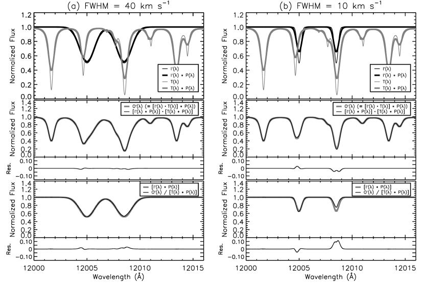
Figure 15: Spectral simulations on the effect of instrumental smearing under telluric absorption. Left: Simulation for a stellar line width of 40 km s^-1. In the top panel, the stellar and telluric spectra are indicated by thin black and gray lines, respectively. Their instrumentally smeared spectra are indicated by thick lines. In the middle panel, the observed spectrum $O^{\prime}(\lambda)$ and the approximated spectrum $[I^{\prime}(\lambda)*P(\lambda)]\cdot[T(\lambda)*P(\lambda)]$ are indicated by thick gray and black lines, respectively. The residual of the two spectra is also shown in the lower part of the middle panel. In the bottom panel, the true stellar spectrum $[I^{\prime}(\lambda)*P(\lambda)]$ and the reproduced spectrum $O^{\prime}(\lambda)/[T(\lambda)*P(\lambda)]$ are indicated with thick gray and thin black lines, respectively. The residual of the two spectra is also shown in the lower part. Right: Spectral simulations, as in the left panels, but for a stellar line width of 10 km s^-1.

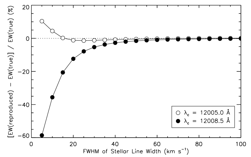
Figure 16: Calculated relative difference in equivalent width between the true spectrum ($[I^{\prime}(\lambda)*P(\lambda)]$) and the reproduced spectrum obtained by telluric correction ($O^{\prime}(\lambda)/[T(\lambda)*P(\lambda)]$) as a function of stellar line width. Open and filled circles indicate, respectively, cases in which stellar lines are half or fully blended with telluric absorption lines. The results are not significantly affected by the stellar line depth.

To summarize, the spectrum produced by the telluric correction ($O^{\prime}(\lambda)/[T(\lambda)*P(\lambda)]$) will diverge significantly from the target’s true spectrum ($[I^{\prime}(\lambda)*P(\lambda)]$) when the following two conditions are fulfilled: (1) the intrinsic width of stellar lines is comparable to or narrower than the instrumental resolution, and (2) the stellar lines are significantly blended with telluric absorption. In such cases, quantitative investigation of the spectrum after telluric correction should be conducted through proper evaluation of the smearing effects or through the use of other approaches such as deconvolution of the observed spectrum with the instrumental profile; this, however, is beyond the scope of this paper.

References

- Beer (1852) Beer. 1852, Annalen der Physik, 162, 78
- Bertaux et al. (2014) Bertaux, J. L., Lallement, R., Ferron, S., Boonne, C., & Bodichon, R. 2014, A&A, 564, A46
- Clough et al. (2005) Clough, S. A., Shephard, M. W., Mlawer, E. J., et al. 2005, J. Quant. Spec. Radiat. Transf., 91, 233
- Cotton et al. (2014) Cotton, D. V., Bailey, J., & Kedziora-Chudczer, L. 2014, MNRAS, 439, 387
- Gullikson et al. (2014) Gullikson, K., Dodson-Robinson, S., & Kraus, A. 2014, AJ, 148, 53
- Hamano et al. (2015) Hamano, S., Kobayashi, N., Kondo, S., et al. 2015, ApJ, 800, 137
- Hamano et al. (2016) —. 2016, ApJ, 821, 42
- Hanson et al. (1996) Hanson, M. M., Conti, P. S., & Rieke, M. J. 1996, ApJS, 107, 281
- Ikeda et al. (2016) Ikeda, Y., Kobayashi, N., Kondo, S., et al. 2016, in Proc. SPIE, Vol. 9908, Ground-based and Airborne Instrumentation for Astronomy VI, 99085Z
- Kausch et al. (2015) Kausch, W., Noll, S., Smette, A., et al. 2015, A&A, 576, A78
- Kurucz (1993) Kurucz, R. L. 1993, SYNTHE spectrum synthesis programs and line data
- Maiolino et al. (1996) Maiolino, R., Rieke, G. H., & Rieke, M. J. 1996, AJ, 111, 537
- Markwardt (2009) Markwardt, C. B. 2009, in Astronomical Society of the Pacific Conference Series, Vol. 411, Astronomical Data Analysis Software and Systems XVIII, ed. D. A. Bohlender, D. Durand, & P. Dowler, 251
- Prugniel et al. (2011) Prugniel, P., Vauglin, I., & Koleva, M. 2011, A&A, 531, A165
- Rothman et al. (2009) Rothman, L. S., Gordon, I. E., Barbe, A., et al. 2009, J. Quant. Spec. Radiat. Transf., 110, 533
- Rudolf et al. (2016) Rudolf, N., Günther, H. M., Schneider, P. C., & Schmitt, J. H. M. M. 2016, A&A, 585, A113
- Seifahrt et al. (2010) Seifahrt, A., Käufl, H. U., Zängl, G., et al. 2010, A&A, 524, A11
- Smette et al. (2015) Smette, A., Sana, H., Noll, S., et al. 2015, A&A, 576, A77
- Taniguchi et al. (2018) Taniguchi, D., Matsunaga, N., Kobayashi, N., et al. 2018, MNRAS, 473, 4993
- Vacca et al. (2003) Vacca, W. D., Cushing, M. C., & Rayner, J. T. 2003, PASP, 115, 389