Agents’ beliefs and economic regimes polarization
in interacting markets

Abstract

In the present paper a model of a market consisting of real and financial interacting sectors is studied. Agents populating the stock market are assumed to be not able to observe the true underlying fundamental, and their beliefs are biased by either optimism or pessimism. Depending on the relevance they give to beliefs, they select the best performing strategy in an evolutionary perspective. The real side of the economy is described within a multiplier-accelerator framework with a nonlinear, bounded investment function. We show that strongly polarized beliefs in an evolutionary framework can introduce multiplicity of steady states, which, consisting in enhanced or depressed levels of income, reflect and reproduce the optimistic or pessimistic nature of the agents’ beliefs. The polarization of these steady states, which coexist with an unbiased steady state, positively depends on that of the beliefs and on their relevance. Moreover, with a mixture of analytical and numerical tools, we show that such static characterization is inherited also at the dynamical level, with possibly complex attractors that are characterized by endogenously fluctuating pessimistic and optimistic levels of national income and price. This framework, when stochastic perturbations are included, is able to account for stylized facts commonly observed in real financial markets, such as fat tails and excess volatility in the returns distributions, as well as bubbles and crashes for stock prices.

Keywords: complex dynamics; bifurcations; multistability; market interactions; heterogeneous beliefs.

The 2008-2009 crisis stimulated new reflections on the origins and the causes of turmoil in the economic environment. Accordingly, it turned out to be relevant the understanding of how instability can reinforce and spread among different sectors, and of what are the factors that may hinder their interaction. As a consequence of such complexity, agents populating the economic system are often better represented as boundedly rational actors, mispricing risks and inappropriately evaluating the economic variables. This is usually at the source of instabilities, that can make the economic system evolve in unpredictable ways, especially when non-deterministic components are acting.
The research goal of the present paper is to improve the understanding of the effect that a biased evaluation of the economic variables may have on the resulting economic dynamics and of whether an increase in the integration between the real and financial sectors is harmful or beneficial to the economy. Relying on analytical investigations complemented by numerical simulations, we study how a boundedly rational agents framework can give rise to multistability phenomena in the economic system, and how the eventual related instability may spread between the integrated markets.

1 Introduction

Seeking the explanations of the 2008-2009 crisis only within the real or the financial side of the economy leads to a dead end way. The global response to the crisis in the form of fiscal stimulus indeed awakened the interest in the multiplier-accelerator approach dating back to [26], from which the modern business cycle theory originated. According to this scheme, endogenous fluctuations spring in the economic activity as a consequence of the mutual interplay between consumption, investments and national income changes, driven either by a multiplicative component that links expenditures to national income (the so-called Keynesian multiplier) or by the principle through which induced investments depend on the pace of growth in the economic activity (the accelerator principle). The original model of [26] has been refined and developed through the decades, emphasizing from time to time different aspects, ranging from the role of the monetary sector or of the inventory adjustment to that of expectations in the national income, or to the effect of bounded investment functions. A burgeoning literature has been widely disseminating: we just mention the contributions in [7, 13, 14, 20, 24, 25].
However, the increasing relevance and influence of the financial side of the economy on the real sector (the so-called phenomenon of financialization of the real economy) can not be neglected, with the consequent need to investigate the interactions between the real and stock subsystems. The related literature can be roughly divided into two research strands, where the former sustains and describes the reverberations of the financial sector into the real one (as in [6, 19, 21, 28]), while the latter, on the contrary, contains a support for the opposite influence direction (see e.g. [1, 18, 19, 21]).

In the wake of the aforementioned discussion, the recent financial crisis strengthened the need to understand the causes of turmoil in the economic environment, keeping a focus on the role of the financial system. Among several factors, a systematic mispricing of risk is commonly regarded as one of the underlying sources of instability for the economic environment. The presence of such a bias, indeed, reflects a boundedly rational behavior of the involved economic actors, who may have a rough knowledge of the economic fundamentals. This can lead agents to systematically overestimate or underestimate them, and to possibly stick to or switch among different forecasting rules on the basis of simple heuristics. It is well-known (see [14]) that bounded rationality together with heterogeneity is a potential source of endogenous fluctuations in the dynamics of the relevant economic variables. An interesting consequence of this modeling framework is also the capability to exhibit simulated time series characterized by several qualitative properties, as leptokurtic returns distributions, large and clustered volatility, that are distinctive features of real time series.

The present contribution belongs to the research strand on the study of interacting markets, and embraces a modelling approach similar to those adopted in [4, 23, 28]. In particular, in each of these works, the sources of complex dynamics are always clearly linked to and explained through particular mathematical phenomena occurring in the model.
For example, in [28] a Keynesian-type goods real market is combined with a stock market populated by heterogeneous fundamentalist and chartist agents. The main result is that the system is characterized by different coexisting steady states, that can become unstable and give rise to complex dynamics. From the mathematical point of view, we have persistent multistability of stable steady states or of attractors characterized by similar degrees of complexity.
Conversely, in [23] it was deeply investigated the effect of coupling either stable and unstable isolated real and stock markets. In this case, a Keynesian good market interacts with a stock market characterized by optimistic and pessimistic agents, whose fractions can change over time according to an evolutionary switching mechanism. Surprisingly, instabilities can not only spread from one market to the other, but they can even arise by increasing the level of interaction between markets that are stable when isolated. From the mathematical viewpoint, this is explained investigating the loss of stability and the kinds of consequent dynamics arising, depending on the degree of interaction or on the degree of optimism/pessimism. Moreover, the analysis of the resulting time series of the economic variables shows a significant deviation from normality.
The work in [4] provides evidence that even a potentially stable economic system can show endogenously fluctuating dynamics, since a locally stable steady state can coexist with other complex attractors, so that the long-run dynamics are strongly path-dependent and can result in sequences of alternating periods of persisting large or small volatility.

In all the above-mentioned papers, the agents’ heterogeneity and their boundedly rational nature have no effects on the set of possible steady states, which always consists of a unique steady state ([23, 4]) or of three coexisting steady states ([28]).
However, it is reasonable to wonder whether the boundedly rational nature of the agents can also affect the final outcomes of the system in terms of existing steady states and their position. In other words, we are interested in inquiring if, as a consequence of a biased evaluation of economic variables, “biased” steady states can emerge. For example, may an excess of optimistic/pessimistic bias foster the emergence of “optimistic” and “pessimistic” steady states, which, in turn, can evolve into optimistic and pessimistic complex attractors? Additionally, to which extent the birth of biased steady states is affected by the markets’ integration?

In order to investigate these aspects, building on the approach pursued in the above mentioned contributions, we analyze an economy made by two, possibly interdependent, subsystems, namely a real and a financial sector. The real sector essentially recalls the economy presented in [4] and [24], in which a multiplier-accelerator model with a bounded investment function is studied, and it is coupled with a stock market populated by optimistic and pessimistic fundamentalists, modeled by following the approach in [23]. In so doing, we shall focus our attention on the degree of interaction between markets, which positively depends on the parameter $\omega\in[0,1],$ as well as we shall take into account the role of agents’ beliefs, represented by a symmetric optimistic/pessimistic bias $b>0,$ and their willingness to switch toward the best performing strategy while operating in the stock market, described by the so-called intensity of choice $\beta>0$ (see e.g. [14]) that regulates the evolutionary selection between forecasting rules. The resulting dynamics are described by a three-dimensional nonlinear system of difference equations for which we analyze the existence and the stability of steady states and, through global analysis, we investigate the presence of multistability phenomena.

The results we come up with can be read under different perspectives. Our most relevant finding concerns the static analysis of the set of possible steady states. We show that, independently of the structural features of the sectors under consideration and of their degree of integration, the steady state final outcomes depend on the optimistic/pessimistic bias and on the intensity of choice of the evolutionary process. If both $b$ and $\beta$ are suitably small, a unique steady state exists, whose position is independent of $b$ and $\beta.$ Conversely, if either $b$ or $\beta$ increases, two new biased steady states emerge, whose position depends on such parameters and which coexist with the previous one. With respect to it, the two new steady states respectively exhibit larger or smaller values in the level of national income and price. This means that in some sense, such final outcomes “keep track” of the optimistic/pessimistic biased belief of the agents, and depart from the unbiased equilibrium. The intuition for the existence of these biased steady states can be read as follows: when the realizations of the true fundamental value of the traded asset are close to some biased beliefs, if the intensity of choice is high enough, then almost all agents will adopt the optimistic or pessimistic predictor, which is the best performing predictor in terms of forecasting error, leading the dynamics to converge to a biased equilibrium. In the same way, when the intensity of choice is sufficiently large, even small differences in predictors’ performances may lead agents to massively switch among forecasting rules. Such alternating waves of optimism and pessimism can drive the system to periodic cycles.
From the mathematical viewpoint, the emergence of additional steady states follows a pitchfork bifurcation, whose consequent multistability is further investigated through global analysis, in order to have a complete picture of the possible dynamical scenarios. The independence of the emergence (but not of the position) of the biased steady states from $\omega$ makes possible that the same economic setting can simultaneously take advantage or be hindered from isolated or fully integrated markets, with a consequent increase in the level of national income and prices, or, conversely, a reduction in the level of national income like, for instance, during a financial shock within an integrated system. The latter framework can be read in the wake of the recent financial crisis where, if on the one hand an integrated economy may facilitate exchange and production through the intermediation of financial instruments, on the other hand no real benefits to the society deriving from the activities of increased financialization may be appraised.

Carrying on the investigation and moving to a dynamical perspective, the analysis we perform allows us to determine the local stability conditions for each steady state, from which we infer a possible ambiguous role for each relevant parameter. Deepening the investigation with the help of numerical simulations, we show that periodic, quasi-periodic and complex dynamics can occur, from a global viewpoint, either when a unique or three steady states exist. Accordingly, oscillations arising in our model are endogenously generated and stoked by the acceleration principle acting in the real subsystem which, in turn, may be triggered by the nonlinearity of the real subsystem, as found in [24] too. In addition, we show the possible coexistence of pairs of complex attractors, arising by the loss of stability of the two new steady states, which give rise to endogenous fluctuations around either the pessimistic or the optimistic steady state. We also find that, even when the fundamental steady state is locally stable, other attractors may coexist with it, making the choice of initial condition crucial for the course of the resulting economic dynamics. Dealing with a purely deterministic version of the model, the convergence toward a particular attractor is determined in advance by the choice of the initial datum. Conversely, when a stochastic version of the model is considered, in which the agents’ demands are buffeted with noise, trajectories can approach different attractors from time to time, so that, for example, periods of persistent optimistic and pessimistic fluctuations can interchange, giving rise to alternating booms and busts. In general, the emergence of stylized facts is mathematically connected with an increasing complexity of the generated dynamics. On the contrary, we show that this is possible in our model even in the presence of stable steady states, when the pitchfork bifurcation occurs. That level of investigation turns out to be relevant to reproduce realistic dynamics observed in the real financial markets together with several stylized facts regarding the return of stock prices (and output as well), such as positive autocorrelation, volatility clustering and non-normal distribution characterized by a high kurtosis and fat tails, with dynamics resulting from the combination of nonlinear forces and random shocks. Therefore, the analytical and numerical results we retrieve from the deterministic framework flow into a better understanding of the stochastic framework.

To summarize, a growing polarization of beliefs gives rise to an increasing richness in the economic regimes that may originate due to the evolutive framework. In such regimes the optimistic and pessimistic hallmark of the belief is not lost but it is mixed up by the complexity of the scenarios, and marks the emerging regimes which are characterized by low, medium or high levels of economic activity.

The remainder of the paper is organized as follows: Section 2 describes the model economy highlighting the features of the two markets; in Section 3 we present the analytical results on the steady states and their local stability; in Section 4 the simulations regarding the deterministic framework as well as the stochastic version of the model are performed and analyzed; in Section 5 we draw some conclusions on our findings; the Appendix gathers all the proofs.

2 The model economy

In the present section we shall introduce the baseline model made up of two interacting sectors, i.e., the real market and the stock market, which are separately outlined in the following subsections. Since the real market we consider essentially consists in the same closed economy taken into account in [4], while the stock market is very close to that depicted in [23], we limit ourselves to report the constitutive and distinctive elements of each market, addressing the interested reader to the above-mentioned works for a more detailed description. In what follows, we are making use of sigmoid functions, namely functions $g:\mathbb{R}\rightarrow\mathbb{R}$ that satisfy the following assumptions:

$$\bullet \,\,\text{vanish at }z=0\text{ and are strictly increasing};$$ (1a)

$$\bullet \,\,\text{are convex on }(-\infty,0]\text{, concave on }[0,+\infty)\text{ and attain maximum slope }1\text{ at }z=0;$$ (1b)

$$\bullet$$ are bounded above and below. (1c)

2.1 The real market

As usual, at each time $t,$ the national income $Y_{t}$ can be expressed through the macroeconomic equilibrium condition

$$Y_{t}=C_{t}+G_{t}+I_{t},$$ (2)

in which we assume constant exogenous government expenditures $G_{t}\equiv\bar{G}$ and aggregate consumption $C_{t}$ depending on autonomous consumption $\bar{C}$ and on the last period national income, setting $C_{t}=\bar{C}+cY_{t-1},$ where $c\in(0,1)$ represents the marginal propensity to consume. Private investments are expressed through

$$I_{t}=\bar{I}+\gamma g_{I}(Y_{t-1}-Y_{t-2})+\omega hP_{t-1},$$ (3)

where $\bar{I}$ are exogenous investments, while the last two terms respectively encompass the accelerator principle and the dependence of the real market on the stock sector, with $\omega\in[0,1]$ representing the degree of interaction between the two markets, $h>0$ the marginal propensity to invest from the stock market wealth and $P_{t-1}$ the price of the financial asset. As noted in [28], a better performance of the financial side of the economy, here encompassed in $P,$ has a beneficial effect on the patrimonial situation of the private sector, promoting greater investments.
Concerning the second term, $\gamma>0$ is the accelerator parameter and $g_{I}:\mathbb{R}\rightarrow\mathbb{R}$ is a function that satisfies assumptions (1). Thanks to assumption (1a), if the national income raises or decline, after a gestation lag, the component of investments depending on national income variation $\Delta Y_{t-1}$ increases or decreases accordingly, by a bounded quantity, thanks to assumption (1c). Finally, thanks to assumption (1b), the effect of both positive and negative national income variations are less and less significant as $|\Delta Y_{t-1}|\rightarrow+\infty,$ attaining its maximum at $\Delta Y_{t-1}=0,$ where the slope coincides with accelerator $\gamma.$ We stress that all the previous aspects are in line with the classic macroeconomic literature of the 1930s-1950s (see e.g. [12, 15, 16]).

Taking into account the expressions for the government expenditure, aggregate consumption and private investments, from (2) we obtain

$$Y_{t}=A+cY_{t-1}+\gamma g_{I}(Y_{t-1}-Y_{t-2})+\omega hP_{t-1},$$

where we defined $A\equiv\bar{C}+\bar{I}+\bar{G}$ as the sum of the autonomous components. We stress that if $\omega=0$ the stock market has no influence on the national income, while if $\omega=1$ the two markets are fully integrated.

2.2 The stock market

We assume that the stock market is populated by fundamentalists, who buy (sell) the asset if its price is lower (higher) than the value estimated as the fundamental asset price but, due to some form of bounded rationality, do not know the true fundamental value of the asset price, trying to form forecasts about it. On the basis of these beliefs, they operate in the stock market. In particular, we suppose there are two groups of fundamentalists: optimists, who typically overestimate the true fundamental asset price, and pessimists, who underestimate it. This approach has been adopted before in [8] and [14], assuming that optimists (resp. pessimists) expect a constant price above (resp. below) the fundamental price. The asset price is set by a market maker on the basis of the following nonlinear adjustment mechanism

$$P_{t}=P_{t-1}+\sigma g_{P}\left(\alpha_{t}D_{t-1}^{O}+\left(1-\alpha_{t}\right)D_{t-1}^{P}\right),$$ (4)

where $\alpha_{t}$ represents the fraction of optimistic fundamentalists, $D_{t-1}^{O}$ and $D_{t-1}^{P}$ denote optimistic and pessimistic demand, respectively, while $\sigma>0$ measures the reactivity of the price variation to aggregate excess demand and $g_{P}:\mathbb{R}\rightarrow\mathbb{R}$ is a function fulfilling assumptions (1). We stress that a similar price adjustment mechanism has been deeply investigated in [22], where it was introduced to prevent an overreaction of price variation to a large excess demand with the consequent unrealistic uncontrolled growth or negativity of prices. In the present contribution, an overreaction would also lead the real sector variables to diverge or to become economically meaningless.

The demand of optimistic and pessimistic agents is proportional to the gap between the estimated fundamental asset price and the realized price, i.e., $D_{t}^{O}=\mu\left(F_{t}^{O}-P_{t}\right),\,D_{t}^{P}=\mu\left(F_{t}^{P}-P_{t}\right),$ where $\mu>0$ represents the agents’ reactivity to such gap. In an environment in which agents, due to their bounded rationality, roughly know the fundamental stock price, they can disagree about the correct value of the fundamental price and can make different estimates on it. In particular, we assume that $F_{t}^{O}=F_{t}^{\ast}+b$ and $F_{t}^{P}=F_{t}^{\ast}-b,$ where $b$ is a positive parameter representing the bias on the fundamental price. On raising $b,$ agents become more and more distant in their beliefs, which are increasingly polarized toward high level of optimism/pessimism. Hence, parameter $b$ also portrays the degree of agents’ heterogeneity.
As concerns the true, unobserved, fundamental value $F^{*}_{t},$ it is described by a weighted average between an exogenous fundamental value $F^{*}$ and an endogenous component proportional to the national income $Y_{t},$ resulting in $F_{t}^{\ast}=(1-\omega)F^{\ast}+\omega dY_{t},$ where $d>0$ captures the strength of the linear dependence between the fundamental value and the current national income level. In this way, $F_{t}^{\ast}$ is linked to the course of the real economy through $\omega\in[0,1],$ i.e., the interaction degree intensity parameter which has been introduced for the investments’ function in (3). It is worth noticing that if $\omega=0$ the true unobserved fundamental value is completely exogenous, while if $\omega=1$ it is endogenously determined by national income, as in [28].

Therefore, the demand functions for both optimists and pessimists become

$$\begin{split}D_{t}^{O}&=\mu\left(\left(1-\omega\right)F^{\ast}+\omega dY_{t}+b-P_{t}\right)\\ D_{t}^{P}&=\mu\left(\left(1-\omega\right)F^{\ast}+\omega dY_{t}-b-P_{t}\right),\end{split}$$

and, replacing them into the price equation (4), we obtain the following expression for the price dynamics

$$P_{t}=P_{t-1}+\sigma g_{P}\big{(}\mu\left(\left(1-\omega\right)F^{\ast}+\omega dY_{t-1}-P_{t-1}+b\left(2\alpha_{t}-1\right)\right)\big{)}.$$

In order to discipline the evolution of the agents’ share employing a certain speculative rule, we assume that a fraction of optimistic agents can switch from period to period to the other behavior, and vice versa. In the present model, differently from [23] and similarly to [5], such an evolutionary process is governed by the squared forecasting error evaluated on the last realization of the fundamental value and of the stock price, namely

$$SE_{t}^{i}=\left(F_{t-1}^{i}-P_{t-1}\right)^{2},\hskip 14.22636pti\in\{O,P\}.$$

Following [2], we assume the fractions evolve according to a multinomial logit rule, that is

$$\alpha_{t}=\frac{e^{-\beta\left(F_{t-1}^{O}-P_{t-1}\right)^{2}}}{e^{-\beta\left(F_{t-1}^{O}-P_{t-1}\right)^{2}}+e^{-\beta\left(F_{t-1}^{P}-P_{t-1}\right)^{2}}},$$

where the positive parameter $\beta,$ also called intensity of choice, measures how fast the mass of optimistic fundamentalists will switch to the optimal prediction strategy. In the limit case $\beta=0$, fractions will be constant and equal to 0.5, and traders never switch strategy; in the other extreme case $\beta\rightarrow+\infty$, in each period all traders use the same, optimal strategy. The latter case represents the highest possible degree of rationality with respect to strategy selection based upon past performance in a heterogeneous agents environment (see [14] for further discussion on the topic). Moreover, $\beta$ also encompasses the agents’ perception of the beliefs relevance. Independently of the moderate or strong polarization of the beliefs (small or large value of $b$), if the agents give a small relevance to them ($\beta$ is small), they will more likely stick to their current forecasting behavior, while if they give a serious consideration to them ($\beta$ is large), their tendency to trust and switch to the best performing belief will result strengthened.

In so doing, the equation that describes the dynamics of the asset price reads as

$$P_{t}=P_{t-1}+\sigma g_{P}\left(\mu\left(\left(1-\omega\right)F^{\ast}+\omega dY_{t-1}-P_{t-1}+b\left(\frac{2}{1+e^{-4b\beta\left(P_{t-1}-\left(1-\omega\right)F^{\ast}-\omega dY_{t-1}\right)}}-1\right)\right)\right).$$

Summarizing, defining $Z_{t}\equiv Y_{t-1}$ in view of the subsequent analysis and taking into account both the real and financial sectors, we can introduce the function $G=(G_{1},G_{2},G_{3}):\mathbb{R}_{+}^{3}\to\mathbb{R}^{3},\,({Y_{t},P_{t},Z_{t}})\mapsto(G_{1}(Y_{t},P_{t},Z_{t}),G_{2}(Y_{t},P_{t},Z_{t}),G_{3}(Y_{t},P_{t},Z_{t})),$ which describes the functioning of the whole economy:

$$Y_{t+1}=G_{1}(Y_{t},P_{t},Z_{t})=A+cY_{t}+\gamma g_{I}(Y_{t}-Z_{t})+\omega hP_{t},$$ (5a)

$$P_{t+1}=G_{2}(Y_{t},P_{t},Z_{t})=P_{t}+\sigma g_{P}\big{(}\mu\left(\left(1-\omega\right)F^{\ast}+\omega dY_{t}-P_{t}+b\left(2\alpha_{t+1}-1\right)\right)\big{)},$$ (5b)

$$Z_{t+1}=G_{3}(Y_{t},P_{t},Z_{t})=Y_{t},$$ (5c)

where

$$\alpha_{t+1}=\dfrac{1}{1+e^{-4b\beta\left(P_{t}-\left(1-\omega\right)F^{\ast}-\omega dY_{t}\right)}}.$$

3 Analytical results on steady states and their stability

In this section we investigate the existence of equilibria for the model in (5), studying the effect on the position and on the stability of the steady states played by the relevant parameters, paying specific attention to the role of the intensity of choice $\beta,$ of the bias $b$ and of the interaction parameter $\omega.$ We start by investigating the number and the expression of possible steady states of the map in (5).

Proposition 1.

System (5) has

• a unique steady state $S^{\ast}=(Y^{\ast},P^{\ast},Z^{\ast})=\left(\frac{A+\omega\left(1-\omega\right)hF^{\ast}}{1-c-\omega^{2}dh},\frac{(1-\omega)(1-c)F^{\ast}+\omega dA}{1-c-\omega^{2}dh},\frac{A+\omega\left(1-\omega\right)hF^{\ast}}{1-c-\omega^{2}dh}\right)$ if

  $$b\leq\frac{1}{\sqrt{2\beta}}.$$ (6)

  Such steady state is well defined for any interaction degree value $\omega\in[0,1]$ provided that

  $$1-c-hd>0.$$ (7)

• three steady states $S^{\ast}=(Y^{\ast},P^{\ast},Z^{\ast}),\,S^{L}=(Y^{L},P^{L},Z^{L})$ and $S^{H}=(Y^{H},P^{H},Z^{H})$ if $b>\frac{1}{\sqrt{2\beta}}.$ In particular, $S^{L}$ and $S^{H}$ are symmetric w.r.t. $S^{\ast},$ which is still well defined for any $\omega$ provided that (7) is fulfilled. Moreover, it holds that $I^{L}<I^{\ast}<I^{H},\,$ for $I\in\{Y,\,P,\,Z\},$ and

  $$\begin{gathered}P_{\ell}=P^{\ast}-\frac{1-c}{1-c-\omega^{2}dh}b<P^{L}<P^{\ast}<P^{H}<P^{\ast}+\frac{1-c}{1-c-\omega^{2}dh}b=P_{h}.\\ Y_{\ell}=Y^{\ast}-\frac{h\omega}{1-c-\omega^{2}dh}b<Y^{L}<Y^{\ast}<Y^{H}<Y^{\ast}+\frac{h\omega}{1-c-\omega^{2}dh}b=Y_{h}.\end{gathered}$$ (8)

  All the components of such new steady states are strictly positive if

  $$b<\min\left\{\dfrac{dA}{1-c},F^{\ast}\right\}.$$ (9)

From Proposition 1, it is possible to have either one or three steady states, whose existence is triggered by sufficiently large values of $\beta$ and $b.$ Steady state $S^{\ast},$ in which $Y^{\ast}$ reduces to the same steady state of the Samuelson model when $\omega=0,$ is in agreement with those found in [4, 21, 23], so that all the comments therein apply to $S^{\ast},$ as well.

We stress that the steady state $S^{\ast}$ represents an unbiased final outcome of the economic system, since it is affected neither by the bias, nor by the evolutionary pressure. Conversely, suitably strong beliefs (namely a suitably strong joint effect of belief polarization and relevance given to them by the agents) trigger the emergence of the two supplementary biased steady states $S^{L}$ and $S^{H}.$ Moreover, recalling (8), $S^{\ast}$ consists in intermediate steady price and national income levels, while $S^{L}$ and $S^{H}$ represent polarized steady states, with respectively small and large steady values. Proposition 1 then shows that sufficiently strong beliefs can drive, independently of the economic setting and its features, the system toward optimistic (like $S^{H}$) or pessimistic (like $S^{L}$) steady states. This result is absent in the related literature, where the only possibilities are given either by a unique steady state ([4, 23]) or by always existing multiple steady states ([28]), which are then independent of the underlying characteristics of the economy and of the agents. In agreement with a Keynesian line of thought, Proposition 1 clearly shows how beliefs, influencing the stock market performance that, in an integrated framework, has in turn a direct influence on the investments, can be the essential cause and driving force that introduces and leads to final outcomes consisting of persistent flourishing or depressed income levels. The optimistic/pessimistic polarization of beliefs, under the evolutionary perspective, reflects on the “sentiment” of the steady states, and can drive the dynamics of the economy toward a more optimistic or pessimistic final output. We stress that also in such situations, the intermediate outcome $S^{\ast}$ is still relevant, as it will become evident from the dynamical analysis, while in [28] it attracts just a set with null measure.

We recall that $b$ encompasses the boundedly rational nature of the agents, while the presence of the switching mechanism, that is crucial as well, is regulated by the parameter $\beta$, that is positively connected to the rationality of the agents in the selection of the forecasting rule, as the larger is the intensity of choice, the larger is the fraction of agents that “rationally” turns to the speculative rule that proved to be the most effective in forecasting the actual stock price. In this sense, we can say that the emergence of the pessimistic and optimistic steady states is fostered by the joint action of an irrational component ($b$) and of a rational component ($\beta$) in agents’ behavior. The roles of $b$ and $\beta,$ which we already noted to be very interconnected from the interpretative point of view, can not be completely disentangled also from the mathematical viewpoint, and we will see that both parameters have a similar influence on the results.

From (8), the optimistic or pessimistic divergence of the biased steady states from the unbiased one is potentially more relevant as the polarization of the beliefs increases. Our next level of investigation is then devoted to study the effect of the main parameters on the steady states position. Since $Z^{i}=Y^{i},\,i\in\{\ast,H,L\}$ and $Z$ has not its own relevance from the economic point of view, we do not deal with it, recalling, however, that it behaves exactly as $Y.$

In order to have the steady state $S^{\ast}$ well defined for any interaction degree value $\omega\in[0,1],$ in the remainder of the paper we shall assume that (7) is fulfilled, even when not explicitly mentioned, as well as we also assume (9) when dealing with $S^{H}$ and $S^{L}$, to guarantee the economic meaningfulness of each steady state value.
In the following comparative static result, we investigate the effects of $b$ and $\beta$ on the steady state values $Y^{i}$ and $P^{i},\,i\in\{\ast,H,L\}.$

Proposition 2.

Under assumption (7), $S^{\ast}$ remains unchanged on increasing $\beta$ or $b.$
Let $b<\min\{dA/(1-c),F^{\ast}\}.$ Then, on increasing $\beta\in(1/(2b^{2}),+\infty),$ we have that $P^{H}$ and $Y^{H}$ are strictly increasing, while $P^{L}$ and $Y^{L}$ are strictly decreasing. Moreover, $\lim_{\beta\rightarrow+\infty}P^{L}(\beta)=P_{\ell}$ and $\lim_{\beta\rightarrow+\infty}P^{H}(\beta)=P_{h},$ $\lim_{\beta\rightarrow+\infty}Y^{L}(\beta)=Y_{\ell}$ and $\lim_{\beta\rightarrow+\infty}Y^{H}(\beta)=Y_{h},$ with $P_{\ell},\,Y_{\ell}$ and $P_{h},\,Y_{h}$ representing respectively the lower and upper bounds defined in (8).
On increasing $b\in(1/{\sqrt{2\beta}},\min\{dA/(1-c),F^{\ast}\}),$ we have that $P^{H}$ and $Y^{H}$ are strictly increasing, while $P^{L}$ and $Y^{L}$ are strictly decreasing.

The comparative static results of Proposition 2 deepen the understating of the effect of the beliefs on the steady states. In Figure 1 we report the evolution of $Y^{L},\,Y^{\ast}$ and $Y^{H}$ on increasing $\beta$ and $b,$ setting $c=d=h=0.5,A=F=10,\omega=1,$ and $b=0.5$ (Figure 1 (A)), $\beta=1$ (Figure 1 (B)). The values of $Y^{L}$ and $Y^{H}$ are obtained numerically solving an implicit equation similar to (17), but in terms of $Y,$ using (16). Indeed, $S^{\ast}$ is neither affected by the intensity of choice nor by the bias. Conversely, not only the existence of $S^{L}$ and $S^{H}$ is affected by $\beta$ and $b,$ but also their values, and in particular their departure from the intermediate steady state $S^{\ast}.$ This means that the stronger are the beliefs (in terms of polarization or intensity of choice), the stronger get the optimistic/pessimistic connotation of the possible final outcomes. In agreement with (8), the maximum possible deviation of $S^{L}$ and $S^{H}$ from $S^{\ast}$ is proportional to the belief polarization and the bounds for $P$ and $Y$ can actually be approached as $\beta\rightarrow+\infty$, that is agents immediately switch to the best performing behavior as if “perfectly rational”.

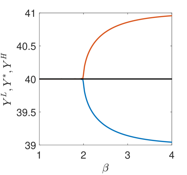
(A)

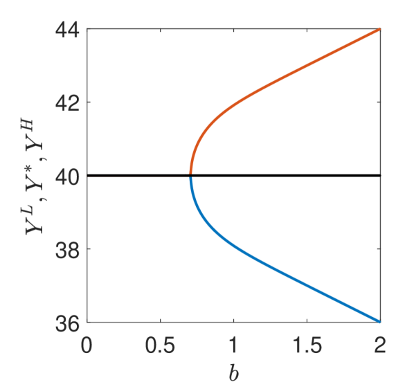
(B)

Figure 1: Steady state national incomes $Y^{L}$ (blue), $Y^{\ast}$ (black) and $Y^{H}$ (red) on varying $\beta$ (plot (A)) and $b$ (plot (B)).

The next proposition studies the effects of $\omega$ on the steady states.

Proposition 3.

Under assumption (7), on increasing $\omega\in[0,1],$ $P^{\ast}$ can be either increasing, decreasing or there exists ${\omega}_{P^{\ast}}\in(0,1)$ such that $P^{\ast}$ decreases on $[0,{\omega}_{P^{\ast}})$ and increases on $({\omega}_{P^{\ast}},1].$ On increasing $\omega\in[0,1],$ $Y^{\ast}$ can be either increasing or there exists ${\omega}_{Y^{\ast}}\in(0,1)$ such that $Y^{\ast}$ increases on $[0,{\omega}_{Y^{\ast}})$ and decreases on $({\omega}_{Y^{\ast}},1].$
Let ${1}/{\sqrt{2\beta}}<b<\min\{dA/(1-c),F^{\ast}\}$ and assume that

$$P^{L}(\omega)\neq P^{\ast}-\frac{1-c}{1-c-{\omega}^{2}dh}\sqrt{b^{2}-\frac{1}{2\beta}},\quad\forall\omega\in(0,1).$$ (10)

Then, on increasing $\omega\in(0,1),$ we have that, for $j\in\{L,H\},$ $P^{j}$ can be either increasing, decreasing or there exists ${\omega}_{P^{j}}\in(0,1)$ such that $P^{j}$ decreases on $(0,{\omega}_{P^{j}})$ and increases on $({\omega}_{P^{j}},1).$ On increasing $\omega\in(0,1),$ for $j\in\{L,H\},$ $Y^{j}$ can be either increasing or there exists ${\omega}_{Y^{j}}\in(0,1)$ such that $Y^{j}$ increases on $(0,{\omega}_{Y^{j}})$ and decreases on $({\omega}_{Y^{j}},1).$

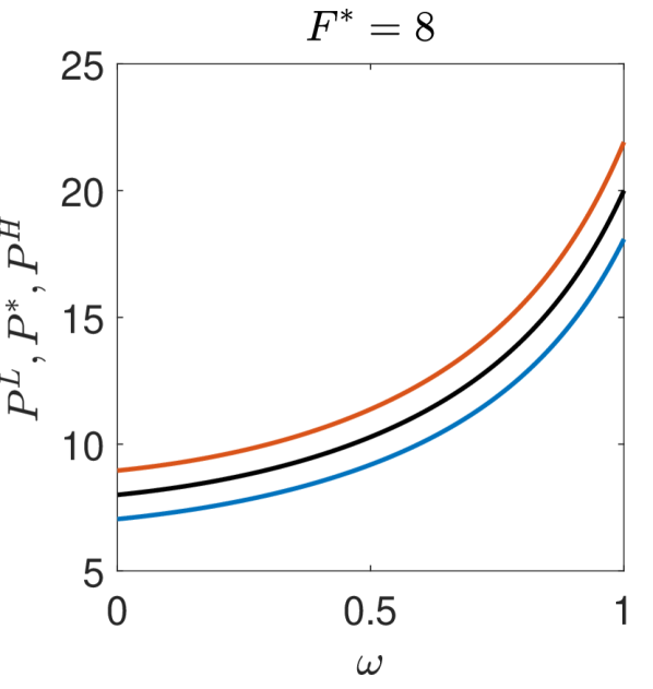
(A)

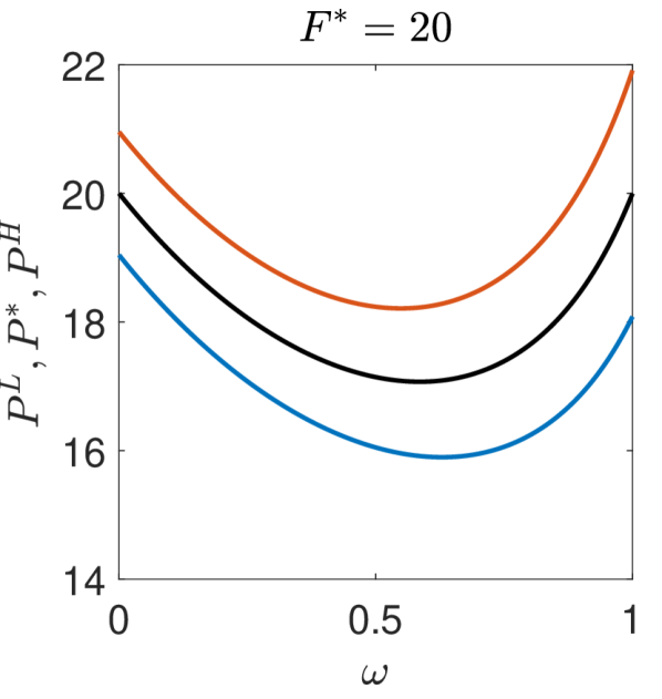
(B)

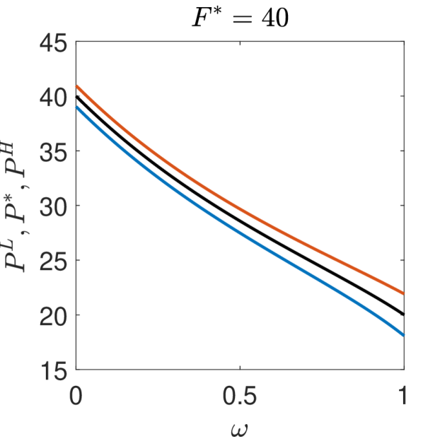
(C)

Figure 2: Steady states $P^{L}$ (blue), $P^{\ast}$ (black) and $P^{H}$ (red) on varying $\omega.$

The previous proposition shows that the effect produced by the degree of interaction between real and stock markets on the steady state values can be quite ambiguous. Since the value of $Y^{\ast}$ is the same as that resulting in [4] in the case of exogenous government expenditure, the unbiased steady national income is either increasing or concave unimodal, reaching a greater value in the case of completely integrated markets than in that of isolated ones (see [4]). Additionally, both optimistic and pessimistic steady national income can be either increasing or concave unimodal as well.

Concerning prices, in Figure 2 we report the evolution with respect to $\omega$ of the steady state values $P^{L},\,P^{\ast}$ and $P^{H}$ setting $A=10,c=d=h=0.5$ and $b=\beta=1,$ for different values of $F^{\ast}.$ We remark that $P^{L}$ and $P^{H}$ are computed numerically solving equation (17) through which they are implicitly defined. On increasing $\omega$ we may have situations in which the more the markets are integrated, the more price increases (Figure 2 (A)), as well as opposite situations in which, increasing the market integration, price is penalized (Figure 2 (C)), with intermediate scenarios in which a partial integration provides the lowest price (Figure 2 (B)). In this last case, we stress a further element of ambiguity: if we compare the steady state values obtained for the same pair of stock and real markets when independent ($\omega=0$) and completely integrated ($\omega=1$), it is not possible to conclude which one has the largest prices. From Figure 2 (B), it is evident that we can simultaneously have all the possible orderings between prices, as $P^{L}(0)>P^{L}(1),P^{\ast}(0)\approx P^{\ast}(1)$ and $P^{H}(0)<P^{H}(1).$
In the rest of the section, we focus on the local stability of the steady states. The first group of results (see Propositions 4–6) deals with $S^{\ast}.$ We start providing analytical conditions under which $S^{\ast}$ is locally asymptotically stable.

Proposition 4.

Under assumption (7), System (5) is locally asymptotically stable at $S^{\ast}$ provided that

$$2b^{2}\beta-1<0$$ (11a)

$$\left(2-E\right)\left(1+c+2\gamma\right)-\omega^{2}dhE>0$$ (11b)

$$1-c+cE+\omega^{2}dhE+\gamma c-E\gamma-E\gamma c+E^{2}\gamma-E^{2}\gamma^{2}+E\gamma^{2}-\gamma>0$$ (11c)

$$2\gamma+c-cE-\gamma E-\omega^{2}dhE<3$$ (11d)

where $E=\mu\sigma(1-2b^{2}\beta).$

Before making explicit from (11) the roles of the interaction degree, of the intensity of choice and of the bias on the stability of $S^{\ast},$ we note that condition (11a) actually coincides with (6), whose violation leads to the emergence of two more steady states. As it will become evident also from the simulations, when $S^{\ast}$ loses stability because of (11a), a pitchfork bifurcation occurs and two stable steady states $S^{L}$ and $S^{H}$ emerge.
We now turn our attention to the roles of $\beta$ and $b$. We highlight that a neutral effect on a steady state is realized when it is locally asymptotically stable/unstable independently of the parameter values; a stabilizing/destabilizing effect occurs when the steady state is locally asymptotically stable only above/below a given threshold value of the considered parameter and unstable otherwise; a mixed effect arises when the steady state is locally asymptotically stable only for intermediate parameter values, between two stability thresholds, and unstable otherwise.

Proposition 5.

Under assumption (7), increasing $b$ or $\beta$ can have a mixed, destabilizing or neutral effect on $S^{\ast}$.

The previous result points out that the bias and the intensity of choice have the same qualitative effect on the stability of $S^{\ast}.$ If the polarization and the relevance of the beliefs is sufficiently increased, $S^{\ast}$ necessarily loses stability. Indeed, from the proof of Proposition 5 we find that $S^{\ast}$ can be unstable for any values of $b$ and $\beta,$ but it cannot be always locally asymptotically stable. The unbiased steady state is then weakened when increasing heterogeneity of the beliefs as it becomes surrounded by the new potentially attracting polarized steady states and because it becomes unstable, although from a static viewpoint its position is not affected by $b$ and $\beta.$ However, as we will see in Section 5, the role of the unbiased steady state, when unstable, may still be significant.

In the following result, we describe the possible stability scenarios arising for $S^{\ast}$ when $\omega$ varies.

Proposition 6.

Under assumption (7), increasing $\omega$ on $[0,1]$ can have a neutral, destabilizing, stabilizing or mixed effect on $S^{\ast}.$

The results obtained in Proposition 6 on the role of $\omega$ are in agreement with those reported in [23], namely the possible scenarios are the same, proving once more the ambiguous role of the interaction degree. It is then not possible to conclude that either encouraging or dampening the integration between the two sides of the economy improves the stability of the markets.

To summarize the findings about the stability of $S^{\ast},$ in Figure 3 we report three different stability regions in the $(\beta,\omega)$-plane, obtained setting $c=d=h=0.38,b=0.5$ and $\mu=1,$ and changing $\sigma$ and $\gamma$ from time to time in order to highlight different stability configurations. Parameters’ combinations for which $S^{\ast}$ is locally asymptotically stable are represented using yellow color, while cyan color is used for the instability region. The stability thresholds corresponding to conditions (11a), (11b) and (11c) are represented by solid, dashed and dotted black lines, respectively.

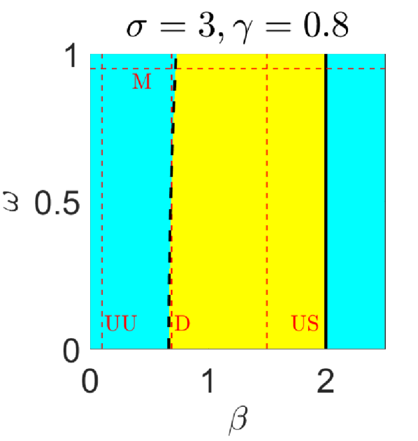
(A)

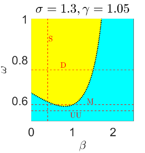
(B)

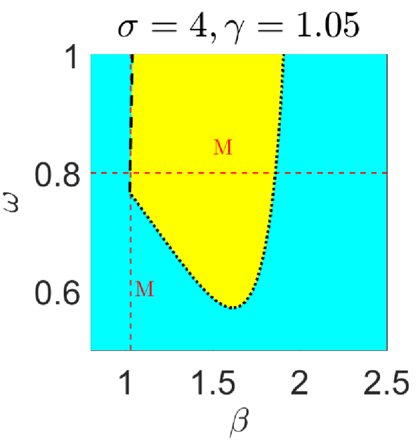
(C)

Figure 3: Stability regions in the $(\beta,\omega)$-plane. Yellow and cyan colors respectively identify parameters’ combinations for which $S^{\ast}$ is locally asymptotically stable and unstable. Solid, dashed and dotted black lines represent stability thresholds, while dashed red lines identify unconditionally unstable (UU), unconditionally stable (US), mixed (M), destabilizing (D) and stabilizing (S) scenarios.

In particular, the region reported in Figure 3 (A) is obtained setting $\sigma=3,\,\gamma=0.8,$ and shows the occurrence, on varying $\omega$, of unconditionally unstable, destabilizing and unconditionally stable scenarios for $\beta=0.1$, $\beta=0.69$ and $\beta=1.5,$ respectively (vertical dashed red lines). On varying $\beta,$ we always find a mixed scenario (e.g. horizontal dashed red line $\omega=0.95$). The stabilizing scenario (vertical dashed red line $\beta=0.4$) on increasing $\omega$ is reported in Figure 3 (B), which is obtained setting $\sigma=1.3$ and $\gamma=1.05.$ On varying $\beta$ we have unconditionally unstable (e.g. when $\omega=0.55$), mixed (e.g. when $\omega=0.58$) and destabilizing (e.g. when $\omega=0.75$) scenarios. Finally, setting $\sigma=4$ and $\gamma=1.05$ we obtain the stability region reported in Figure 3 (C), in which we underline the occurrence of mixed scenarios both on varying $\omega$ (e.g. for $\beta=1.03$) and $\beta$ (e.g. for $\omega=0.8$). The previous considerations allow concluding that each scenario predicted by Propositions 5 and 6 is actually possible. We stress that the mixed scenarios on varying $\beta$ pointed out in each of Figures 3 (A)–(C) are obtained crossing different couplings of thresholds.

In the next proposition we show the possible effects of $\omega$ and $\beta$ on the local asymptotic stability of $S^{H}$ and $S^{L},$ provided that they exist and are positive.

Proposition 7.

Let assumptions (7) and (9) hold true. If, keeping $\omega$ fixed and increasing $\beta,$ for $S^{\ast}$ we have
$\bullet$ a destabilizing scenario, then on increasing $\beta\in(1/(2b^{2}),+\infty)$ we can either have a stabilizing or an unconditionally stable scenario on $S^{H}$ and $S^{L};$
$\bullet$ a mixed scenario, then on increasing $\beta\in(1/(2b^{2}),+\infty)$ we can either have a destabilizing or a mixed scenario on $S^{H}$ and $S^{L};$
$\bullet$ an unconditionally unstable scenario, then $S^{H}$ and $S^{L}$ are unconditionally unstable, too.
Moreover, on increasing $\omega,$ there is a one to one correspondence between the scenarios for $S^{\ast}$ for $\beta<1/(2b^{2})$ and those for $S^{H}$ and $S^{L}$ for $\beta>1/(2b^{2}).$

The previous proposition shows that the stability of $S^{L}$ and $S^{H}$ is strongly connected to that of $S^{\ast}.$ From the mathematical point of view, we actually have that the stability behavior of $S^{L}$ and $S^{H}$ is a “specular reflection” of that of $S^{\ast}$ with respect to $\beta=1/(2b^{2}).$ Decreasing $\beta$ has the same effect on the stability of $S^{\ast}$ of increasing it on the stability of $S^{L}$ and $S^{H}.$ Thanks to Proposition 7, we can highlight a substantial difference with the scenarios of the economic setting reported in [23]: in the present case, for increasing values of the intensity of choice, when $S^{\ast}$ loses stability (both in the destabilizing and in the mixed scenarios) we can still have convergence toward a steady state. Such framework occurs when $S^{\ast}$ undergoes a pitchfork bifurcation and the new steady states $S^{L}$ and $S^{H}$ are locally stable. This means that, in such scenario, the final outcome is always a steady state, which, even if it changes, may be locally stable. The most extreme situation is realized when a destabilizing scenario for $S^{\ast}$ is followed by an unconditionally stable one for $S^{L}$ and $S^{H}.$ Accordingly, convergence toward a steady state may occur for any value of $\beta.$

4 Numerical simulations

In this section we present the results of several numerical investigations, collected pursuing a double aim. Firstly, we wish to complement the analysis of Section 3. In particular, we want to understand what kinds of dynamics occur when $S^{\ast}$ becomes unstable, as well as to investigate the possible scenarios arising with the emergence of $S^{L}$ and $S^{H}.$ Secondly, we want to study the qualitative properties of the time series when exogenous non-deterministic effects are taken into account, that is, considering a stochastically perturbed version of the model, in agreement with [4, 11, 23]. In continuity with Section 3, we focus on the effect of the degree of interaction $\omega$ and of the intensity of choice $\beta.$

In order to perform simulations, we need to specify the analytical expressions of $g_{I}$ and $g_{P}.$ In what follows, we use the same sigmoid function considered in [3], i.e.,

$$g_{X}(z)=\begin{cases}a_{1}^{X}\tanh\left(\dfrac{z}{a_{1}^{X}}\right)&\text{ if }z\geq 0,\\ a_{2}^{X}\tanh\left(\dfrac{z}{a_{2}^{X}}\right)&\text{ if }z<0,\end{cases}$$ (12)

where $X\in\{I,P\}$ and $a_{1}^{X},a_{2}^{X}$ are positive parameters, with $a_{1}^{X}$ as upper bound when $z\to+\infty$ and $-a_{2}^{X}$ as lower bound when $z\to-\infty$. A straightforward check shows that function $g_{X}$ belongs to $\mathcal{C}^{2}(\mathbb{R})$ and satisfies assumptions (1). In all the simulations reported in the present section we set $F=A=15$, $c=d=h=0.38$, $b=0.5$ and $\mu=1.$
Concerning the upper and lower bounds $a_{i}^{X},\,i\in\{1,2\},$ of functions $g_{I}$ and $g_{P},$ we start by recalling that the steady state values of $P$ and $Y$ significantly change on varying $\omega.$ Since such bounds represent the maximum possible positive or negative variation of $P_{t}$ and $Y_{t},$ it is reasonable to assume that they are qualitatively connected to the magnitude of prices and national incomes. In fact, it makes economic sense to think that investments and prices can not grow indefinitely but that, instead, their variation is linked to the pace of economic activity, reflected in the level of prices and national income, which are in turn connected to the amount of resources existing in a certain country. To encompass such fact into the simulations, we let $a_{i}^{X}$ proportionally change depending on the value of the steady state $S^{\ast},$ setting $a_{1}^{P}=2P^{\ast}/F,\,a_{2}^{P}=4P^{\ast}/F,\,a_{1}^{I}=3Y^{\ast}(1-c)/A$ and $a_{2}^{I}=6Y^{\ast}(1-c)/A.$ In this way, for $\omega=0$ we have $a_{1}^{P}=2,\,a_{2}^{P}=4,\,a_{1}^{I}=3,\,a_{2}^{I}=6,$ while they increase/decrease, on varying $\omega,$ proportionally to $P^{\ast}$ and $Y^{\ast}$ (see Proposition 3). We recall that we checked the robustness of the simulations by varying all the parameters in suitable ranges, obtaining results that are qualitatively comparable with those reported in the next subsections. We also point out that the reported two-dimensional bifurcation diagrams are obtained setting the same initial datum for each parameters’ coupling. Conversely, in order to highlight coexistence, one-dimensional bifurcation diagrams are all obtained “following the attractor”. This means that, having a strictly increasing or decreasing sequence of parameters $a_{i}$, $i=1,\dots,m,$ we set the initial datum for the first simulation equal to $a_{1},$ while the initial datum for the simulation with $a_{i+1}$ is set suitably close to the solution of the simulation obtained with $a_{i}$.

4.1 Deterministic simulations

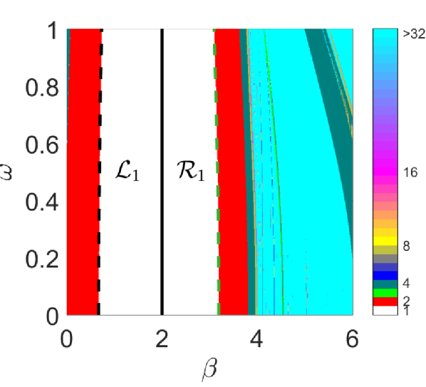
(A)

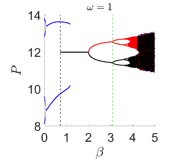
(B)

Figure 4: Simulations obtained setting $\sigma=3$ and $\gamma=0.8.$ (A): Two-parameters bifurcation diagram. White color identifies parameters’ combinations for which the initial datum converges toward a steady state, other colors are used for attractors consisting of more than a single point (cyan is used for attractors consisting of more than 32 points). Black lines denote the stability thresholds of $S^{\ast},$ while the green line denotes the stability threshold of $S^{H}.$ (B): Bifurcation diagrams for $P$ on varying $\beta$ when $\omega=1.$ Different colors correspond to different initial conditions.

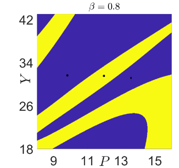
(A)

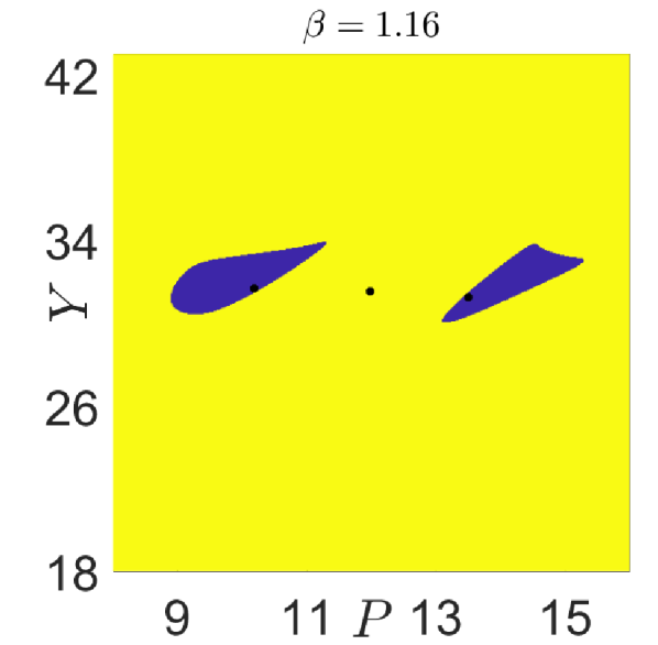
(B)

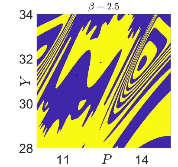
(C)

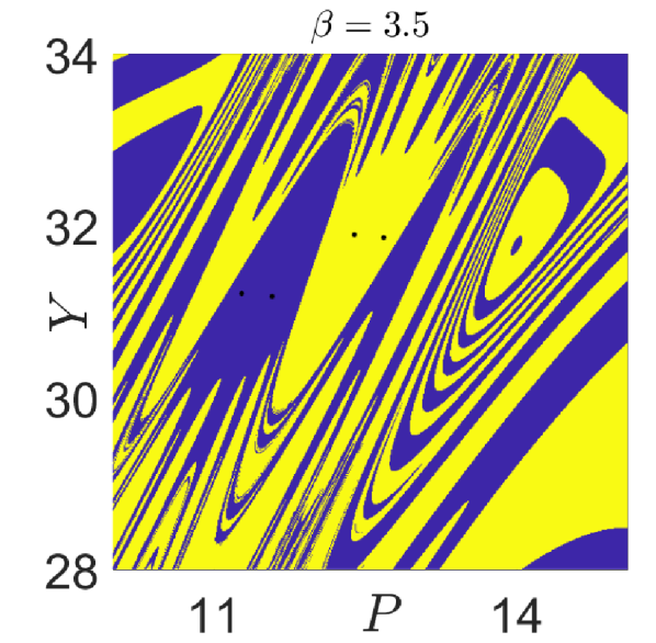
(D)

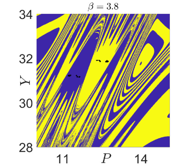
(E)

(F)

Figure 5: Evolution of the basins of attraction on varying the intensity of choice $\beta$. In (A)-(B) the basins of attraction of the steady state $S^{\ast}$ is represented in yellow together with the basin of the coexisting 2-cycle, in violet. Panel (C) refers to the basins of the biased steady states $S^{L}$ and $S^{H}$ whose birth is due to the occurrence of the pitchfork bifurcation which makes the unbiased steady state $S^{\ast}$ unstable. In panel (D) the basins of the two 2-cycles arising at the destabilization of $S^{L}$ and $S^{H}$ are depicted, which then turn into chaotic attractors due to a cascade of further period-doubling bifurcations for increasing values of $\beta$, as panels (E)-(F) show.

We shall now explain the functioning of the model by considering different sets of simulations, which provide a portrait of the possible dynamics that may occur in our model economy, emphasizing how the relevant parameters affect the evolution of the economic variables. In particular, we aim to account for the richness of the possibly complex dynamical behaviors arising in unstable regimes, which however keep evident track of the simple distinctive characterization of the beliefs, in terms of optimistic/pessimistic bias.
In the first set of simulations we set $\sigma=3$ and $\gamma=0.8,$ and the resulting stability region for $S^{\ast}$ is that reported in Figure 3 (A). In Figure 4 (A) we show the two-dimensional bifurcation diagram in the $(\beta,\omega)$-plane, where each point is represented using a different color depending on the number of points of the attractor that was approached starting by the initial datum $(Y_{0},P_{0},Z_{0})=(Y^{\ast}+0.001,P^{\ast}+0.001,Z^{\ast}+0.001)$ after $T=10000$ iterations. In particular, white color denotes parameter combinations for which convergence is toward a one-point attractor, i.e., a steady state, red color is used for period-2 cycles, cyan color for attractors consisting of more than 32 points (namely, high period cycles, chaotic attractors or closed invariant curves), and the remaining colors for cycles with periods between 3 and 32. Black solid and dashed lines respectively represent the stability thresholds corresponding to (11a) and (11b), delimiting the region within which (see also the yellow set in Figure 3 (A)) the steady state $S^{\ast}$ is stable and dynamics converge toward it (white region $\mathcal{L}_{1}$). If we start from any $(\beta,\omega)\in\mathcal{L}_{1}$ and we increase $\beta,$ we exit the stability region $\mathcal{L}_{1}$ as $S^{\ast}$ crosses the black solid line, but in the white region $\mathcal{R}_{1}$ dynamics again converge toward a steady state. In fact, according to Propositions 1 and 4, such black line, whose equation is given by $\beta=2$ since $b=0.5$, represents both the bound for the stability condition (11a) for $S^{\ast}$ and the threshold to the left/right of which we have a unique/three coexisting steady states. As a consequence, when the solid line $\beta=2$ is crossed on increasing $\beta$, the steady state $S^{\ast}$ becomes unstable by means of a pitchfork bifurcation and the two stable steady states $S^{L}$ and $S^{H}$ arise. We stress that, with the present choice of the initial datum, dynamics converge toward $S^{H}$ for all $(\beta,\omega)\in\mathcal{R}_{1}.$

Region $\mathcal{R}_{1}$ is the specular of $\mathcal{L}_{1}$ with respect to $\beta=2.$ In particular, the green dashed line is obtained starting from the black dashed threshold line and numerically solving the implicit equations used in the proof of Proposition 7. This, in agreement with Proposition 7, confirms that region $\mathcal{R}_{1}$ is the region of local asymptotic stability for $S^{H}.$

As remarked in the comments to Figure 3 (A), on increasing $\beta$ we have mixed scenarios for $S^{\ast}$ for any $\omega.$ From Proposition 7, since the right stability threshold for $S^{\ast}$ is described by the “pitchfork” condition (11a), this is the only situation in which a mixed scenario for $S^{\ast}$ “translates” into a destabilizing scenario for $S^{H}.$ As described after Proposition 7, this is simply due to the fact that, crossing $\beta=2$ from right to left, $S^{H}$ disappears. In fact, starting from any $(\beta,\omega)\in\mathcal{R}_{1},$ for increasing values of $\beta$ we cross the green stability threshold, while decreasing $\beta$ we leave $\mathcal{R}_{1}$ entering $\mathcal{L}_{1}.$ To be more precise about the possible dynamics occurring when steady states lose stability, we can see that when we leave both $\mathcal{L}_{1}$ and $\mathcal{R}_{1}$ crossing a dashed stability threshold, we enter one of the red regions, meaning that dynamics, previously converging to a steady state, now converge to a period-2 cycle.
In Figure 4 (B) we report three bifurcation diagrams obtained for $\omega=1$. The blue bifurcation diagram is obtained setting $(Y_{0},P_{0},Z_{0})=(Y^{\ast}+0.001,P^{\ast}+0.001,Z^{\ast}+0.001)$ and on varying $\beta$ between $0$ and $1.17,$ while the red and the black bifurcation diagrams are obtained respectively setting $(Y_{0},P_{0},Z_{0})=(Y^{\ast}+0.001,P^{\ast}+0.001,Z^{\ast}+0.001)$ and $(Y_{0},P_{0},Z_{0})=(Y^{\ast}-0.001,P^{\ast}-0.001,Z^{\ast}-0.001),$ and on varying $\beta$ between $0.73$ and $5.$

We can see that as long as $\beta<0.728$ (black dashed line), but close to such value, dynamics converge toward a period-2 cycle which attracts almost all the trajectories. Such period-2 cycle coexists with the stable steady state $S^{\ast}$ on an interval of values of $\beta,$ and then the former disappears when its basin of attraction shrinks and is absorbed by that of the steady state. This coexistence is also reported in Figures 5 (A)-(B) where the basin of attraction of $S^{\ast}$ is represented in yellow while the basin of the 2-cycle is depicted in violet. The two panels show that, as $\beta$ grows, the basin of the 2-cycle reduces in size and for further increases of the intensity of choice parameter there is a contact between the periodic points and their basin boundary leading to the disappearance of the 2-cycle.
From the red and the black bifurcation diagrams of Figure 4 (B), it is evident the pitchfork bifurcation occurring at $\beta=2$ with the red and the black lines springing from $S^{\ast}$ that respectively represent $S^{H}$ and $S^{L}$ (see Figure 5 (C), which reports the basins of attraction of the steady states born via the pitchfork bifurcation). These are the biased steady states, whose birth via pitchfork bifurcation can be read as the effect of agents’ decision when the intensity of choice is high enough. In this case almost all agents adopt the optimistic or pessimistic predictor, which is the best performing predictor in terms of forecast error, leading the dynamics to converge to an equilibrium different from $S^{\ast}.$ We stress that, according to Proposition 2, all components of $S^{H}$ and $S^{L}$ are respectively increasing and decreasing with respect to $\beta.$ If $\beta$ is further increased, they both lose stability through a flip bifurcation and then a cascade of period-doubling bifurcations leads to chaos. In fact, from Figure 4 (D) on we observe the basins of attraction of the couple of 2-cycles born when $S^{L}$ and $S^{H}$ lose stability. It is also worth remarking that Proposition 7 guarantees that the first period-doubling bifurcation occurs for the same $\beta$ value both for $S^{L}$ and $S^{H},$ and Figure 4 (B) suggests that the subsequent period-doubling bifurcations are simultaneous, too. Still increasing $\beta$ has the effect of making these 2-cycles unstable, leading to the emergence of chaotic attractors (see Figures 4 (E)-(F)) associated with erratic dynamics in the course of price and national income. In this scenario, on increasing $\beta,$ the intermediate unbiased steady state loses its relevance when becomes unstable, as almost all trajectories converge toward the optimistic or the pessimistic attractor.

We now focus on the role of the degree of interaction $\omega$, considering vertical sections of the bifurcation diagram in Figure 4 (A). The destabilizing scenario for both $S^{\ast}$ and $S^{H}$ only leads to the emergence of a period-2 cycle (e.g. for $\beta=0.7$). It is worth noticing that the possible effects on $S^{H}$ of increasing the interaction degree when $\beta>2$ are again specular with respect to those on $S^{\ast}$ when $\beta<2.$ In fact, we can identify neutrally stable (e.g. for $\beta=2.5$) or unstable (e.g. for $\beta=4$) scenarios, as well as destabilizing scenarios (e.g. for $\beta=3.2$).

The second family of simulations we consider is obtained setting $\sigma=1.3$ and $\gamma=1.05.$ The corresponding stability region for $S^{\ast}$ is depicted in Figure 3 (B) and the corresponding two-dimensional bifurcation diagram is reported in Figure 6 (A), in which the dotted black line represents the stability threshold (11c). Differently from the first set of simulations, condition $\beta=2$ (represented using blue color) acts no more as a stability threshold, but it still shapes regions in which we have either one or three steady states. The initial datum is always set equal to $(Y_{0},P_{0},Z_{0})=(Y^{\ast}+0.001,P^{\ast}+0.001,Z^{\ast}+0.001)$ and in region $\mathcal{R}_{2}$ the convergence is toward $S^{H},$ while in region $\mathcal{L}_{2}$ convergence is toward $S^{\ast}.$
In this case, we can have either convergence toward a steady state (in regions denoted by $\mathcal{L}_{2}$ and $\mathcal{R}_{2}$) or toward an attractor consisting of more than $32$ points (cyan regions). Both couple of regions are specular with respect to the vertical blue line $\beta=2,$ in agreement with Proposition 7, and, depending on the value of the interaction degree, unconditionally unstable, mixed and destabilizing scenarios for $S^{\ast}$ respectively correspond to unconditionally unstable, mixed and stabilizing scenarios for $S^{H}.$ This means that the emergence of new steady states makes possible to have convergence toward a stable steady state as $\beta\rightarrow+\infty.$

If we start from $(\beta,\omega)\in\mathcal{L}_{2}$ and we increase (or, depending on $\omega,$ also if we decrease) $\beta$, the crossing of the black dotted line makes $S^{\ast}$ unstable and immediately trajectories converge toward an attractor consisting of more than 32 points (represented by cyan color). The same happens in relation to $S^{H}$ if we start from $(\beta,\omega)\in\mathcal{R}_{2}$ and we decrease (or, depending on $\omega,$ also if we increase) $\beta,$ crossing the green dotted line (which, like in Figure 4 (A), is obtained starting from the black dotted threshold and numerically solving the implicit equations used to prove Proposition 7). This stability loss for $S^{\ast}$ and $S^{H}$ is associated with the occurrence of Neimark-Sacker bifurcations, as it looks evident evident also from Figure 6 (B), where we report three bifurcation diagrams on varying $\beta$ for $\omega=0.575,$ which highlight the presence of a mixed scenario for both $S^{\ast}$ and $S^{H}$. We stress that we checked that qualitatively similar results are obtained for all the values of $\omega$ for which a mixed scenario arises.

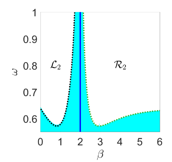
(A)

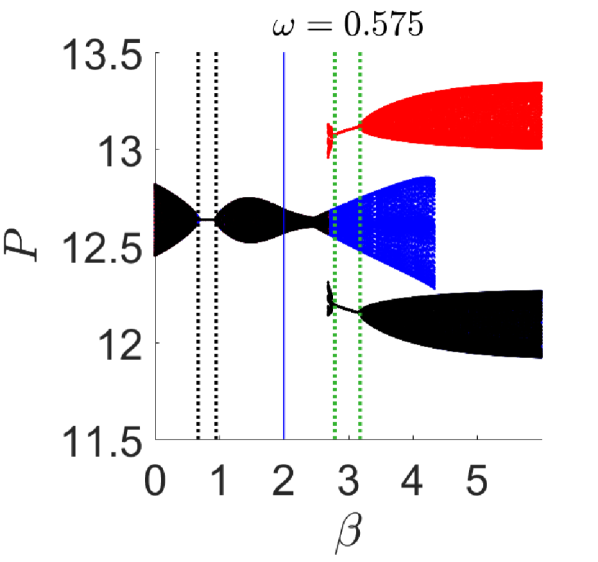
(B)

Figure 6: Simulations obtained setting $\sigma=1.3$ and $\gamma=1.05.$ (A): Two-parameters bifurcation diagram. White color is used to identify parameters’ combinations for which the initial datum converges toward a steady state, cyan is used for attractors consisting of more than 32 points. The black dotted line represents the stability threshold of $S^{\ast}$ while the green dotted line refers to the stability threshold of $S^{H}.$ (B): Bifurcation diagrams for $P$ on varying $\beta$ when $\omega=0.575.$ Different colors correspond to different initial conditions.

The blue bifurcation diagram, obtained setting $(Y_{0},P_{0},Z_{0})=(Y^{\ast}+0.001,P^{\ast}+0.001,Z^{\ast}+0.001)$ and increasing $\beta$ from $0$ to $6,$ lies below the red one, obtained setting $(Y_{0},P_{0},Z_{0})=(Y^{\ast}+0.001,P^{\ast}+0.001,Z^{\ast}+0.001)$ and decreasing $\beta$ from $6$ to $0,$ which in turns lies above the black one, obtained setting $(Y_{0},P_{0},Z_{0})=(Y^{\ast}-0.001,P^{\ast}-0.001,Z^{\ast}-0.001)$ and decreasing again $\beta$ from $6$ to $0$.
We numerically checked that the closed invariant curve, arising from the stability loss of $S^{\ast}$, attracts almost any trajectory also for intensity of choice values $\beta>2$ suitably close to $2$, when steady states $S^{H}$ and $S^{L}$ already exist but are unstable (black bifurcation diagram, just to the right of the blue dotted line). Such closed invariant curve coexists, as $\beta$ increases, first with another couple of closed invariant curves (blue, red and black bifurcation diagrams just to the left of the first green dotted line), then with $S^{H}$ and $S^{L}$ (blue, red and black bifurcation diagrams between the two green dotted lines) and finally again with another couple of closed invariant curves (blue, red and black bifurcation diagrams just to the right of the second green dotted line).
Similar considerations hold also when the destabilizing scenario for $S^{\ast}$ is followed by the stabilizing one for $S^{H}$ and $S^{L}.$ Once more, the common aspect is the coexistence of attractors encompassing optimistic, pessimistic or unbiased levels in the economic variables, with the addition of the magenta attractor in which each piece embodies large or small levels too. On varying $\omega,$ from vertical sections of Figure 6 (A) we infer that we can have either stabilizing scenarios for both $S^{\ast}$ (e.g. for $\beta=1$) and $S^{H}$ (e.g. for $\beta=3$) or unconditionally unstable scenarios for both $S^{\ast}$ and $S^{H},$ when $\beta$ is sufficiently close to $2.$

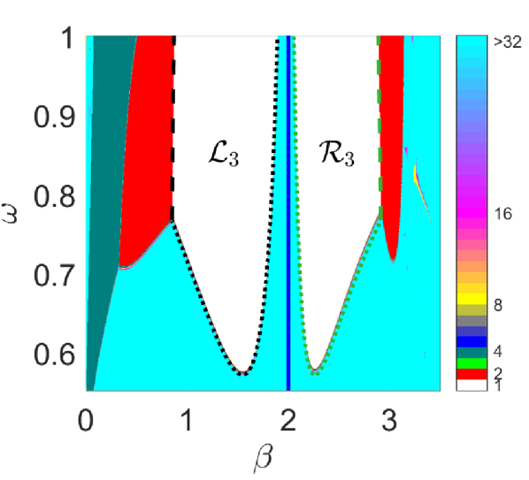
(A)

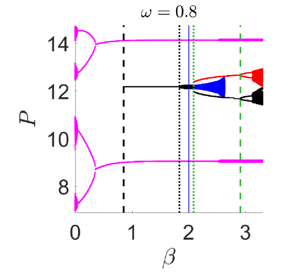
(B)

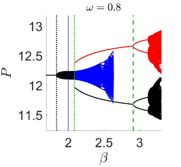
(B)

Figure 7: Simulations obtained setting $\sigma=4$ and $\gamma=1.05.$ (A): Two-parameters bifurcation diagram. White color is used to identify parameters’ combinations for which the initial datum converges toward a steady state, other colors are used for attractors consisting of more than a single point (cyan is used for attractors consisting of more than 32 points). Black lines represent stability thresholds of $S^{\ast},$ green lines stability thresholds of $S^{H}.$ (B): Bifurcation diagrams for $P$ on varying $\beta$ when $\omega=0.8.$ Different colors correspond to different initial conditions. (C): blow up of plot (B).

The last family of simulations, whose two-dimensional bifurcation diagram is reported in Figure 7 (A), is obtained setting $\sigma=4$ and $\gamma=1.05,$ and the corresponding stability region is that reported in Figure 3 (C). The initial datum is the same as in the first two sets of simulations and, when dynamics converge for $\beta>2,$ we have convergence toward $S^{H}.$ All the previous considerations about the specular stability/instability regions and stability thresholds for $S^{\ast}$ and $S^{H}$ with respect to $\beta=2$ still hold. On varying $\beta$, we can have either unconditionally unstable or mixed scenarios for both $S^{\ast}$ and $S^{H}$ but, differently from the first two families of simulations, the convergence toward the steady states may be replaced, when the aforementioned steady states become unstable, by convergence toward different kinds of attractors for different values of the interaction degree parameter $\omega$. This is perceivable looking at the stability thresholds for $S^{\ast}$ reported in Figure 7 (A). The black dotted curve corresponds to condition (11c), crossing which we enter the cyan region, in which attractors consist of more then 32 points (actually, it is a closed invariant curve and the stability loss of $S^{\ast}$ occurs through a Neimark-Sacker bifurcation), while the black dashed line corresponds to condition (11b), crossing which we enter the red region, in which the attractor is a period-2 cycle. The same holds for the green stability thresholds for $S^{H},$ too, which also in this case are obtained from the black thresholds and numerically solving the implicit equations used in the proof of Proposition 7.

In the four bifurcation diagrams reported in Figures 7 (B)-(C) we study the occurring dynamics when $\omega=0.8.$ The blue bifurcation diagram is obtained setting $(Y_{0},P_{0},Z_{0})=(Y^{\ast}+0.001,P^{\ast}+0.001,Z^{\ast}+0.001)$ and increasing $\beta$ from $1.5$ to $2.65;$ the red one is obtained setting $(Y_{0},P_{0},Z_{0})=(Y^{\ast}+0.001,P^{\ast}+0.001,Z^{\ast}+0.001)$ and decreasing $\beta$ from $3.3$ to $0.855;$ the black one is obtained setting $(Y_{0},P_{0},Z_{0})=(Y^{\ast}-0.001,P^{\ast}-0.001,Z^{\ast}-0.001)$ and decreasing $\beta$ from $3.3$ to $0.855;$ the magenta one is obtained setting $(Y_{0},P_{0},Z_{0})=(Y^{\ast}+0.001,P^{\ast}+0.001,Z^{\ast}+0.001)$ and increasing $\beta$ from $0$ to $3.3.$ As $S^{\ast}$ turns unstable on decreasing $\beta$ (when the black dashed line is crossed), the steady state is replaced by a 2-cycle, similarly to what happens in the first family of simulations. However, as $S^{\ast}$ becomes unstable on increasing $\beta$ (when there is a crossing of the black dotted line), the steady state is replaced by a closed-invariant curve. The attractor arising from the stability loss of $S^{\ast}$ then coexists with the stable steady states $S^{L}$ and $S^{H}.$ Further increasing $\beta,$ when such two steady states become unstable (green dashed line), a flip bifurcation occurs. The subsequent period-2 cycles lose stability through a Neimark-Sacker bifurcation.
The magenta attractor exists for the whole range of values of $\beta$ we consider. If we decrease $\beta$ from $0.854$ to $0,$ such attractor firstly evolves toward a period-4 cycle and then a Neimark-Sacker bifurcation occurs. If we increase $\beta$ starting from $0.854,$ each of the two points composing the attractor is replaced by a closed invariant curve. As $\beta$ increases, we have that the attractor originated by the loss of stability of $S^{\ast}$ (blue bifurcation diagram) coexists with steady states $S^{L}$ and $S^{H},$ with a closed invariant curve, and with a period-2 cycle (magenta bifurcation diagram), giving rise to a quite articulated multistability situation made by qualitatively different attractors. Once more, the common aspect is the coexistence of attractors encompassing optimistic, pessimistic or unbiased levels in the economic variables, with the addition of the magenta attractor in which each piece embodies large or small levels, too.

The previous considerations confirm and enrich the analytical results about local stability. From a qualitative point of view, we can not speak about a unique type of mixed scenario, as those arising from the simulations above are significantly different. The first relevant difference can be highlighted in correspondence of the loss of stability of $S^{\ast}$ for increasing values of $\beta$, namely when the rightmost stability threshold is violated. In the example reported in Figure 4, the stable steady state $S^{\ast}$ loses stability through a pitchfork bifurcation, and hence the new attractor has the same complexity as the previous one, even if it has a different interpretation from the economic point of view. In the example reported in Figures 6 and 7, dynamics converging to $S^{\ast}$ are replaced by quasi-periodic dynamics, that is, by an attractor of different complexity, even if arisen from $S^{\ast}.$ The second difference can be highlighted in correspondence to the loss of stability of $S^{\ast}$ as $\beta$ decreases, when the leftmost stability threshold is violated. In this case, the unique steady state is again $S^{\ast},$ but different dynamics are possible, as the stability can be lost through a “simple” period-2 cycle or through more complex quasi-periodic dynamics. We stress that, for the same parameter values describing the stock and the real economy, different dynamics can arise on changing the degree of interaction. However, even in the presence of a very articulated range of complex situations, all the dynamic scenarios can be still traced back to the static setting outlined in Proposition 1, and hence easily read in terms of the effects of beliefs.

4.2 Stochastic simulations

The deterministic analysis has revealed that, starting from a situation in which the fundamental steady state is locally stable, an increase in the parameter $\beta$ generates the onset of endogenous fluctuations as well as the rise of multistability phenomena. The goal of this part is to show that a stochastic version of our model is able to generate varied and realistic dynamics, as observed in real financial markets, such as bubbles and crashes for stock prices and fat tails and excess volatility in the distributions of returns. In the presence of exogenous noise (on investors’ demands) and, accordingly, of fundamental shocks to the price dynamics, periods of high volatility in the price course may alternate with periods in which prices do not depart too much from the fundamental value. Such behavior may arise when the parameter setting is located near the pitchfork bifurcation boundary and exogenous noise can occasionally spark long-lasting endogenous fluctuations around the new steady states.
Therefore the model is modified along the following lines. The demand placed by the two groups of agents is set as

$$D_{t}^{X}=\mu(F_{t}^{X}-P_{t})+\varepsilon_{t}^{X},\,X\in\{O,P\},$$ (13)

where $\varepsilon_{t}^{X}$ are sequences of independent, identically distributed random normal variables, with zero mean and variance $s_{X}^{2}$. These random disturbances may reflect errors in investors’ decision making processes, heterogeneity within the same group, or they may capture the idea that it is quite difficult for investors to determine the fundamentals (in fact fundamental values may change over time due to real shocks), as already argued by [17].
Plugging the perturbed demands into the price equation (4) and acting as in Section 2, we end up with

$$P_{t}=P_{t-1}+\sigma g_{P}\left(\mu\left(\left(1-\omega\right)F^{\ast}+\omega dY_{t-1}-P_{t-1}+b\left(\frac{2}{1+e^{-4b\beta\left(P_{t-1}-\left(1-\omega\right)F^{\ast}-\omega dY_{t-1}\right)}}-1\right)\right)+\varepsilon_{t}\right),$$ (14)

where $\varepsilon_{t}$ is is a sequence of independent, identically distributed random normal variables, with zero mean and variance $s^{2}=(\varepsilon_{t}^{O}+\varepsilon_{t}^{P})^{2}/(2\mu)^{2}$.
In analyzing the stochastic version of our model, we aim at showing that several stylized facts of financial markets may be retrieved that, in turn, can possibly affect the behavior of the real sector. Thanks to their apparent explanatory power, models that have been being developed with interacting agents and interconnected sectors are increasingly used as tools for economic policy recommendations (see e.g. [9, 11, 27]).
In what follows, we consider the price returns, defined as

$$R_{t}=\log(P_{t})-\log(P_{t-1}),$$

focusing, at first, on the deviation from normality of their distribution. In all the simulations reported in this subsection we employ the same parameter setting adopted for Figure 4.

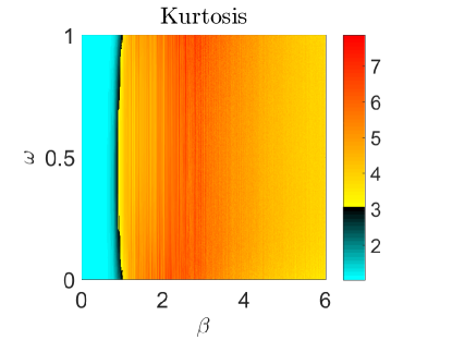
Figure 8: Kurtosis of returns distribution in the $(\beta,\omega)$-plane. Different colors are associated with different kurtosis values, according to the colors bar. The distributions of returns exhibits the fat-tail property (with more probability mass in the tails than warranted by a normal distribution with identical mean and standard deviation) with the highest kurtosis levels obtained for values of the intensity of choice $\beta$ roughly between $2$ and $4$.

Figure 8 displays the values of the kurtosis in the distributions of the log-returns as the parameters $\beta$ and $\omega$ jointly vary. We observe that, independently of the degree of interaction between the two markets, as the intensity of choice increases from 2 to 4, the kurtosis increases as well, reaching values that reveal a non-normal distribution of the log-returns. In fact, kurtosis measures how fat the tails of the distributions are compared to the ones of a normal distribution. In this respect, to observe fat tails it is essential to have trajectories in which prices move frequently far from their average and, in turn, this is related to the behavior of the intensity of choice $\beta$. For example, looking at Figure 4, we observe that, as $\beta$ increases, coexisting attractors appear, due to the occurrence of the pitchfork bifurcation, and this reflects into a large kurtosis, e.g. for $2<\beta<4$ roughly. As $\beta$ increases further, the bifurcation diagram of Figure 4 shows that the dynamics turn into chaotic and this translates into slightly reduced values for the kurtosis in the log-returns of the stochastic version of the model. Such results are confirmed also by the top and bottom left panels of the Figure 9, obtained for $\omega=0$ and $\omega=1,$ respectively. As the degree of market interaction grows, the switching between the optimistic and pessimistic strategies towards the best performing rule is able to increase the kurtosis in the distributions of the log-returns.
Another peculiar stylized fact of returns’ times series is the volatility clustering, namely, the occurrence of several consecutive periods characterized by high volatility alternated with others characterized by low volatility. This is graphically evident from the central panels of Figure 9, in which a typical example of time series of returns, obtained for the parameter setting used for Figure 4 and $s=0.15\,P^{\ast}/F$, is reported. Finally, volatility clustering is highlighted by the typical strongly positive, slowly decreasing autocorrelation coefficients of absolute returns, reported in the right top and bottom panels of Figure 9.
Overall, we may come up with the conclusion that the stochastic version of our model with interacting real and financial sectors is able to replicate key empirical regularities of actual stock markets. In particular, the functioning of the stochastic version of the model descends from the functioning of its deterministic counterpart. In the deterministic setup, endogenous dynamics arise when a model parameter crosses the Neimark-Sacker bifurcation boundary, as well as coexisting attractors appear when the pitchfork bifurcation takes place. In the stochastic version, when the two non-fundamental steady states appear and are still locally stable, the interplay of nonlinear elements and random shocks leads to realistic dynamics.

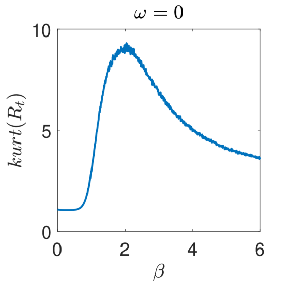
(A)

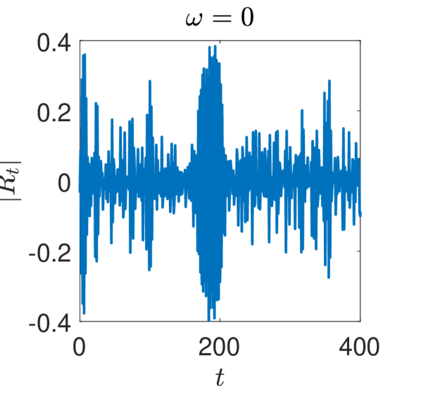
(B)

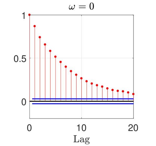
(C)

(D)

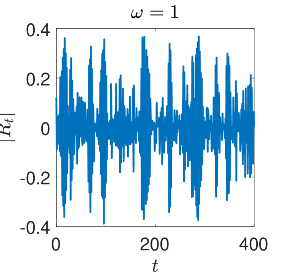
(E)

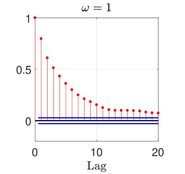
(F)

Figure 9: The left column represents the evolution of kurtosis when $\omega=0$ (A) and $\omega=1$ (D), the central column plots the time series of absolute returns exhibiting phases of high volatility alternating with phases of low volatility either for $\omega=0$ (B) or $\omega=1$ (E), the right column shows the autocorrelation function for absolute returns for $\omega=0$ (C) and $\omega=1$ (F) obtained for $\beta=6$, revealing evidence for volatility clustering.

5 Conclusions

The proposed model shows that beliefs can influence the possible final outcomes of an economy not only in terms of increasing the complexity in the possible endogenous dynamics of the economic variables, but also in a more constitutive way. From the static point of view, strongly heterogeneous expectations can alter the set of steady states, originating strongly polarized multiple steady states that in turn reflect the optimism/pessimism of the beliefs. This can then dynamically evolve into complex attractors still characterized by optimism/pessimism of the beliefs, provided that such bias is strong and relevant enough. To sum up, it is certainly evident the role played by the occurrence of the pitchfork bifurcation, with the optimistic/pessimistic steady states common to the various sets of simulations. But this is not the sole effect. From a broader perspective, the occurrence of such biased steady states coexisting with the unbiased one is the result of the repeated strategies’ evaluation made by the agents, which may lead the economy to converge to high, intermediate or low, steady or endogenously fluctuating, levels of national income (and prices as well), with the consequent richness of dynamical behaviors related to all equilibria and their eventual destabilization.
The investigation, performed with a mix of analytical, numerical and empirical tools, has a twofold aim: besides understanding the influence of the beliefs on the course of the economy in terms of possible final outcomes and stability of the desired equilibrium level of national income and prices, we are interested in the role of market integration and in its possible beneficial effect on the overall economy in terms of increasing level of national income. We showed that an increase of market interaction may be either beneficial, as it may increase the national income of the economy, or it may generate a contraction in its level, as no real benefits to the society deriving from the activities based on an increased integration may be appraised. The potential beneficial effect of the degree of interaction seems to emerge also from the local stability analysis, with the found stabilizing effect of the interaction degree for suitable values of the intensity of choice parameter, which measures agents’ reactivity toward the best performing strategy. This interplay between interaction, imitation and beliefs is crucial also in view of understanding and interpreting the stylized facts that our model is able to reproduce when buffeted with stochastic noise, like the recurrent boom-bust phenomena observed in the real financial markets together with several stylized facts regarding stock price returns, such as positive autocorrelation, volatility clustering and non-normal distribution characterized by a high kurtosis and fat tails.
The proposed model belongs to a class of models that, we believe, may be useful in order to interpret and understand the recent developments in the increasingly interconnected economy, which constitutes a true challenge for regulatory measures which seek to appease abrupt market fluctuations. We hope that our work will stimulate further investigations in such direction, especially as concerns the deepening of the understanding of the role of the agents’ beliefs. The financial crisis at the end of the last decade has not only made evident that our comprehension of the dynamics of real and financial markets is still incomplete, but it has also revealed how important is to intensify the research activity in this field.

Appendix A Proofs of Propositions

Proof of Proposition 1.

In order to find the steady states, we set $P_{t+1}=P_{t}=P,\,Y_{t+1}=Y_{t}=Y$ and $Z_{t+1}=Z_{t}=Z$ in (5). From (5c) we have $Z=Y.$ Inserting it in (5a) and (5b) since, recalling (1a), we have that $g_{I}(0)=0$ and that $g_{P}(z)=0$ is solved by $z=0$ only, we obtain

$$Y=A+cY+\omega hP,$$ (15a)

$$\left(1-\omega\right)F^{\ast}+\omega dY-P+b\left(\frac{2}{1+e^{-4b\beta\left(P-\left(1-\omega\right)F^{\ast}-\omega dY\right)}}-1\right)=0.$$ (15b)

The steady state existing independently of $\beta$ and $b$ is found setting $P=\left(1-\omega\right)F^{\ast}+\omega dY,$ which immediately provides $(Y,P,Z)=(Y^{\ast},P^{\ast},Z^{\ast})=S^{\ast},$ whose components, by (7), are positive independently of $\omega.$

In order to verify the existence of additional steady states, we notice that, from (15a), national income $Y$ can be rewritten as a function of the asset price $P$ as

$$Y=\dfrac{A+\omega hP}{1-c}.$$ (16)

Inserting such expression in (15b), we find the following equation in $P,$ whose solutions are the steady state values of price:

$$\left(1-\frac{\omega^{2}dh}{1-c}\right)P-\left(1-\omega\right)F^{\ast}-\frac{\omega dA}{1-c}+b-\frac{2b}{1+e^{-4b\beta\left(\left(1-\frac{\omega^{2}dh}{1-c}\right)P-\left(1-\omega\right)F^{\ast}-\frac{\omega dA}{1-c}\right)}}=0.$$ (17)

Defining

$$f_{1}(P)\equiv\left(1-\frac{\omega^{2}dh}{1-c}\right)P-\left(1-\omega\right)F^{\ast}-\frac{\omega dA}{1-c}+b$$ (18)

and

$$f_{2}(P)\equiv\frac{2b}{1+e^{-4b\beta\left(\left(1-\frac{\omega^{2}dh}{1-c}\right)P-\left(1-\omega\right)F^{\ast}-\frac{\omega dA}{1-c}\right)}}\,,$$ (19)

we observe that $f_{1}$ is a straight line that crosses the horizontal axis of the Cartesian coordinate plane at the point $P_{\ell}=\frac{\left(1-c\right)\left(1-\omega\right)F^{\ast}+\omega dA-\left(1-c\right)b}{1-c-\omega^{2}dh}$ and the vertical axis at $f_{1}(0)=b-\left(1-\omega\right)F^{\ast}-\frac{\omega dA}{1-c}.$ We stress that such points can be either positive or negative and that the function $f_{1}$ is increasing in $P$. In fact, thanks to the positivity condition for the steady state $P^{\ast},$ we have $1-\frac{\omega^{2}dh}{1-c}>0.$
Simple computations allow to conclude that $f_{2}$ is an increasing function in $P$ and it has an inflection point at $P=P^{\ast}$, it is convex for $P\in\left(-\infty,\,P^{\ast}\right)$ and concave for $P\in\left(P^{\ast},\,+\infty\right).$ Moreover, $f_{2}(P)$ crosses the vertical axis at the point $f_{2}(0)=\frac{2b}{1+e^{4b\beta\left(\left(1-\omega\right)F^{\ast}+\frac{\omega dA}{1-c}\right)}}$. We always find $f_{1}\left(P^{\ast}\right)=f_{2}\left(P^{\ast}\right)$ and, according to the values assumed by the model parameters, $f_{1}$ and $f_{2}$ can also meet at some points $P^{L}$ and $P^{H},$ with $P^{L}\in\left(P_{\ell},\,P^{\ast}\right)$ and $P^{H}\in\left(P^{\ast},\,P_{h}\right),$ where $P_{h}$ is the intersection point between the horizontal line $g(P)=2b$ and $f_{1}(P).$ Recalling the expression of $P^{\ast},$ it is easy to see that $P_{\ell}$ and $P_{h}$ respectively correspond to the left and right bounds for $P$ in (8). In order to determine the bounds on $Y,$ it is possible to proceed as done for $P,$ obtaining an equation like (17) from (15), this time in terms of $Y.$
More precisely, since $f_{1}$ is an increasing straight line and $f_{2}$ is an increasing function in $P$, with an inflection point at $P=P^{\ast},$ being convex for $P\in\left(-\infty,\,P^{\ast}\right)$ and concave for $P\in\left(P^{\ast},\,+\infty\right),$ then if $f_{1}^{\prime}(P^{\ast})\geq f_{2}^{\prime}(P^{\ast})$ we have exactly one solution to (17), that is, $P=P^{\ast},$ while if $f_{1}^{\prime}(P^{\ast})<f_{2}^{\prime}(P^{\ast})$ we have exactly three distinct solutions, $P^{L},\,P^{\ast}$ and $P^{H},$ to (17). We notice that $f_{1}^{\prime}(P^{\ast})<f_{2}^{\prime}(P^{\ast})$ corresponds to

$$1-\frac{\omega^{2}dh}{1-c}<2b^{2}\beta\left(1-\frac{\omega^{2}dh}{1-c}\right),$$

which, recalling (7), reduces to (6).

To guarantee the economic meaningfulness of $P^{H}$ and $P^{L},$ we require their positivity. A sufficient condition to ensure this consists in setting $P_{\ell}>0,$ which is verified for each $\omega\in[0,1]$ when $b(1-c)<\min\{dA,F^{\ast}(1-c)\}.$ Since $f_{2}(P)$ is strictly positive and $f_{1}(P)$ is strictly increasing, their intersection is realized for $P>0.$

Finally, it is easy to show that $f_{1}$ and $f_{2}$ are symmetric w.r.t. $P=P^{\ast},$ i.e., that $f_{i}(P^{\ast}+\varepsilon)-f_{i}(P^{\ast})=f_{i}(P^{\ast})-f_{i}(P^{\ast}-\varepsilon),$ for every $\varepsilon>0$ and $i\in\{1,2\}.$ For $f_{1}$ that is true because it is a straight line, while for $f_{2}$ a direct computation shows that $f_{2}(P^{\ast}+\varepsilon)-f_{2}(P^{\ast})=f_{2}(P^{\ast})-f_{2}(P^{\ast}-\varepsilon)=b\bigl{(}e^{4b\beta\varepsilon(1-\frac{\omega^{2}dh}{1-c})}-1\bigr{)}/\bigl{(}e^{4b\beta\varepsilon(1-\frac{\omega^{2}dh}{1-c})}+1\bigr{)}.$

We then have that, when (6) holds, (17) is solved not only by $P^{\ast},$ but also by $P^{L}$ and $P^{H},$ symmetric values w.r.t. $P^{\ast}.$ From (16) and since in the steady states we have $Z=Y,$ it follows that national income positively depends on the asset price and thus to $P^{L}$ and $P^{H}$ correspond $Y^{L}$ and $Y^{H},$ with $Y^{L}<Y^{\ast}<Y^{H},$ as well as $Z^{L}$ and $Z^{H},$ with $Z^{L}<Z^{\ast}<Z^{H}$. Moreover, if $P^{H}$ and $P^{L}$ are positive, then, from (16) , $Y^{H},Y^{L},Z^{H}$ and $Z^{L}$ are positive, too. Finally, by the linearity of (16) and by the symmetry of $P^{L}$ and $P^{H}$ w.r.t. $P^{\ast},$ it follows that $Y^{L}$ and $Y^{H}$ are symmetric w.r.t. $Y^{\ast},$ and, since in the steady states we have $Z=Y,$ then $Z^{L}$ and $Z^{H}$ are symmetric w.r.t. $Z^{\ast}.$ This concludes the proof. ∎

Proof of Proposition 2.

We start noting that, from (16), $Y$ positively depends on $P$, so it is sufficient to study the monotonicity for $P$ on varying either $\beta$ or $b$. Setting

$$W=\left(1-\frac{\omega^{2}dh}{1-c}\right)P-\left(1-\omega\right)F^{\ast}-\frac{\omega dA}{1-c},$$ (20)

we may rewrite (17) as

$$W+b=\frac{2b}{1+e^{-4b\beta W}},$$ (21)

from which it follows that

$$e^{-4b\beta W}=\frac{b-W}{b+W}.$$ (22)

Moreover, it holds that

$$W=\frac{1-c-\omega^{2}dh}{1-c}(P-P^{\ast}).$$ (23)

For $W\in(-b,b)$ on both sides of equation (22) there are positive, strictly decreasing functions of $W$ and the rhs of (22) is also independent of $\beta.$ In what follows, we make reference to some explanatory plots reported in Figure 10.

Firstly we consider $P^{H}(\beta).$ From (8) we have that $W^{H}(\beta),$ defined by (23), belongs to $(0,b).$ Setting $W\in(0,b),$ the lhs of (22) is decreasing with respect to $\beta$, so that if $\beta_{1}<\beta_{2}$ we find $e^{-4b\beta_{1}W}>e^{-4b\beta_{2}W}.$ An illustrative example is reported in Figure 10 (A), from which it is evident that the last inequality guarantees that the unique solution $W^{H}(\beta)$ of (22) on $(0,b)$ increases with $\beta$, and hence, recalling (23), $P^{H}(\beta)$ increases, too. We proceed in a similar way for $P^{L}$. From (8), we have that $W^{L}(\beta),$ defined by (23), belongs to $(-b,0).$ Setting $W\in(-b,0)$, the lhs of  (22) is increasing with respect to $\beta,$ so that if $\beta_{1}<\beta_{2}$ we find $e^{-4b\beta_{1}W}<e^{-4b\beta_{2}W}$. An illustrative example is reported in Figure 10 (B), from which it is evident that the last inequality guarantees that the unique solution $W^{L}(\beta)$ of (22) on $(-b,0)$ decreases with $\beta$, and hence, recalling (23), $P^{L}(\beta)$ decreases, too. The two limits of $P^{j},\,j\in\{H,L\},$ as $\beta\rightarrow+\infty$ can be easily obtained by noting that the lhs of (22) pointwise approaches $0$ for each $W\in(0,b),$ so that $W^{H}(\beta)$ tends to $b,$ and the lhs of (22) pointwise approaches $+\infty$ for each $W\in(-b,0),$ so that $W^{L}(\beta)$ tends to $-b.$ Using (23) allows concluding. For the limits of $Y^{j},\,j\in\{H,L\},$ it is sufficient to compute the limit as $\beta\rightarrow+\infty$ of the rhs of (16), in which we replace $P$ with either $P^{H}$ or $P^{L}$ and we use the just computed limits.

To study the monotonicity of $P^{L}(b)$ and $P^{H}(b)$ with respect to $b$, we rewrite (22) as

$$e^{-4\beta W}=\left(\frac{b-W}{b+W}\right)^{1/b},$$ (24)

which is well defined on $W\in(-b,b)$ and shares the solutions with (23). The lhs is represented by a positive, strictly decreasing function of $W.$ Let us consider $b_{1}<b_{2}$ and the corresponding steady states $P^{H}(b_{1})$ and $P^{H}(b_{2})$. From (8) we have that $W^{H}(b_{1})$ and $W^{H}(b_{2}),$ defined by (23), respectively belong to $(0,b_{1})$ and $(0,b_{2}).$ For $W\in(0,b_{1})$, noting that $\frac{b_{1}-W}{b_{1}+W}<\frac{b_{2}-W}{b_{2}+W}$, we find $\left(\frac{b_{1}-W}{b_{1}+W}\right)^{1/b_{1}}<\left(\frac{b_{2}-W}{b_{2}+W}\right)^{1/b_{2}}.$ An illustrative example is reported in Figure 10 (C), from which it is evident that the last inequality allows concluding that if $W^{H}(b_{2})\in(0,b_{1})$ it holds that $W^{H}(b_{1})<W^{H}(b_{2})$ (indeed, also if $W^{H}(b_{2})\in[b_{1},b_{2}),$ since we have $W^{H}(b_{1})\in(0,b_{1})$). This implies that $W^{H}(b)$ increases with $b$, and hence, recalling (23), $P^{H}(b)$ increases, too.

Now we turn our attention to $P^{L}(b_{1})$ and $P^{L}(b_{2}),$ still assuming $b_{1}<b_{2}$. From (8) we have that $W^{L}(b_{1})$ and $W^{L}(b_{2}),$ defined by (23), respectively belong to $(-b_{1},0)$ and $(-b_{2},0).$ For $W\in(-b_{1},0)$, noting that $\frac{b_{1}-W}{b_{1}+W}>\frac{b_{2}-W}{b_{2}+W}$, we find $\left(\frac{b_{1}-W}{b_{1}+W}\right)^{1/b_{1}}>\left(\frac{b_{2}-W}{b_{2}+W}\right)^{1/b_{2}}.$ An illustrative example is reported in Figure 10 (D), from which it is evident that the last inequality allows concluding that if $W^{L}(b_{2})\in(-b_{1},0)$ it holds that $W^{L}(b_{1})>W^{L}(b_{2})$ (indeed, also if $W^{L}(b_{2})\in(-b_{2},-b_{1}]$, since we have $W^{L}(b_{1})\in(-b_{1},0)$). This implies that $W^{L}(b)$ decreases with $b$, and hence, recalling (23), $P^{L}(b)$ decreases, too.

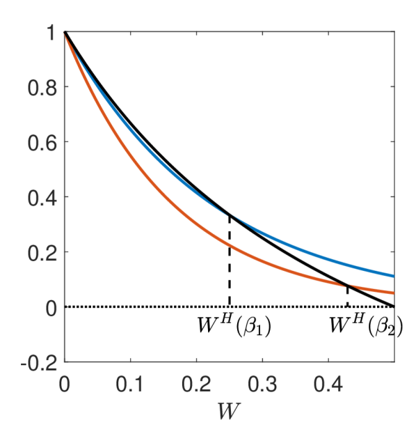
(A)

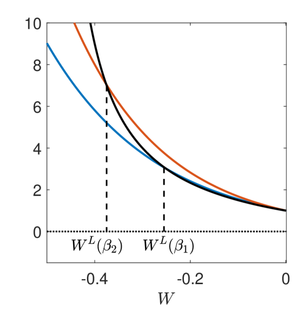
(B)

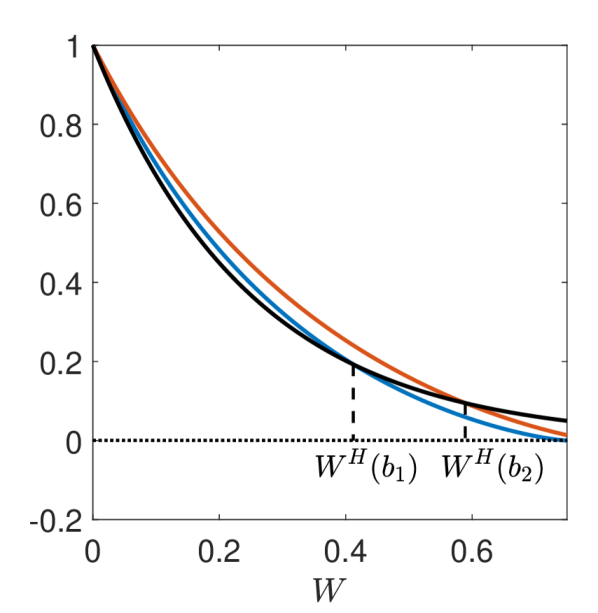
(C)

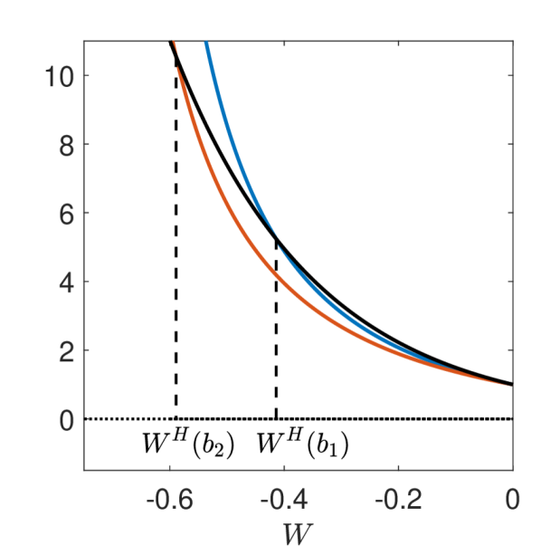
(D)

Figure 10: (A), (B): Intersections between the function representing the rhs of (22) (black) and two functions representing the lhs of (22) respectively for $\beta=\beta_{1}$ (blue) and $\beta=\beta_{2}>\beta_{1}$ (red), when $W\in(0,b)$ (plot (A)) and $W\in(-b,0)$ (plot (B)). (C),(D): Intersections between the function representing the lhs of (24) (black) and two functions representing the rhs of (24) respectively for $b=b_{1}$ (blue) and $b=b_{2}>b_{1}$ (red), when $W\in(0,b_{1})$ (plot (C)) and $W\in(-b_{1},0)$ (plot (D)).

∎

Proof of Proposition 3.

Let us start focusing on the effects of $\omega$ on $P^{\ast}.$ A direct computation shows that

$$\frac{\partial P^{\ast}}{\partial\omega}=\frac{dh(dA-F^{\ast}(1-c))\omega^{2}+2dhF^{\ast}(1-c)\omega+(1-c)(dA-F^{\ast}(1-c))}{(1-c-\omega^{2}dh)^{2}}.$$

Such derivative is non-negative for each $\omega\in[0,1]$ when $dA-F^{\ast}(1-c)\geq 0$ and in this case $P^{\ast}$ increases with $\omega,$ for every $\omega.$ When instead $dA-F^{\ast}(1-c)<0,$ the numerator of ${\partial P^{\ast}}/{\partial\omega}$ may become negative. More precisely, ${\partial P^{\ast}}/{\partial\omega}>0$ is equivalent to $dh(F^{\ast}(1-c)-dA)\omega^{2}-2dhF^{\ast}(1-c)\omega+(1-c)(F^{\ast}(1-c)-dA)<0.$ When the discriminant of $dh(F^{\ast}(1-c)-dA)\omega^{2}-2dhF^{\ast}(1-c)\omega+(1-c)(F^{\ast}(1-c)-dA)=0$ is non-positive, we have that $P^{\ast}$ decreases with $\omega,$ for each $\omega\in[0,1].$ When instead the discriminant is positive, it is easy to show that there are two positive solutions $\omega_{1,2}$ to such equation, and the larger between them always exceeds $1.$ Hence, if the smallest solution $\omega_{1}$ is larger than 1, then $P^{\ast}$ decreases with $\omega,$ for each $\omega\in[0,1].$ If instead $\omega_{1}$ lies in $(0,1),$ then $P^{\ast}$ decreases with $\omega$ on $[0,\omega_{1})$ and increases with $\omega$ on $(\omega_{1},1].$ Setting ${\omega}_{P^{\ast}}=\omega_{1},$ we obtain the desired result on $P^{\ast}.$
As concerns $Y^{\ast},$ a direct computation shows that

$$\frac{\partial Y^{\ast}}{\partial\omega}=\frac{h(\omega^{2}dhF^{\ast}+2\omega(dA-F^{\ast}(1-c))+F^{\ast}(1-c))}{(1-c-\omega^{2}dh)^{2}}.$$

Such derivative is positive for each $\omega\in[0,1]$ when $dA-F^{\ast}(1-c)\geq 0$ and in this case $Y^{\ast}$ increases with $\omega,$ for every $\omega.$ When instead $dA-F^{\ast}(1-c)<0,$ the numerator of ${\partial Y^{\ast}}/{\partial\omega}$ may become negative. More precisely, when the discriminant of $\omega^{2}dhF^{\ast}+2\omega(dA-F^{\ast}(1-c))+F^{\ast}(1-c)=0$ is non-positive, we have that $Y^{\ast}$ increases with $\omega,$ for each $\omega\in[0,1].$ When instead the discriminant is positive, it is easy to show that there are two positive solutions $\omega_{3,4}$ to such equation, and the largest between them always exceeds $1.$ Hence, if the smallest solution $\omega_{3}$ is larger than 1, then $Y^{\ast}$ increases with $\omega,$ for each $\omega\in[0,1].$ If instead $\omega_{3}$ lies in $(0,1),$ then $Y^{\ast}$ increases with $\omega$ on $[0,\omega_{3})$ and decreases with $\omega$ on $(\omega_{3},1].$ Setting ${\omega}_{Y^{\ast}}=\omega_{3},$ we obtain the desired result on $Y^{\ast}.$

Let us now assume ${1}/{\sqrt{2\beta}}<b<\min\{dA/(1-c),F^{\ast}\},$ namely (6) is violated and (9) holds true, so that the two additional steady states $0<P^{L}(\omega)<P^{H}(\omega)$ exist for every $\omega\in[0,1].$ In order to analyze their behavior with respect to increasing values of $\omega,$ we use the implicit function theorem. Let $f:(0,+\infty)\times(0,1)\rightarrow\mathbb{R},\,(P,\omega)\mapsto f(P,\omega),$ be defined by the lhs of (17) and let $P:(0,1)\rightarrow(0,+\infty),\,\omega\mapsto P(\omega),$ be the function which associates to $\omega\in(0,1)$ one of the solutions implicitly defined by $f(P,\omega)=0$ for $b>1/\sqrt{2\beta}$. Recalling the definition of $W$ in (20), we then have

$$\frac{\partial f}{\partial P}=\frac{(1-c-dh\omega^{2})(1+2(1-4b^{2}\beta)e^{-4b\beta W}+e^{-8b\beta W})}{(1-c)(e^{-4b\beta W}+1)^{2}}$$

and

$$\frac{\partial f}{\partial\omega}=\frac{(-Ad+F-Fc-2Pdh\omega)(1+2(1-4b^{2}\beta)e^{-4b\beta W}+e^{-8b\beta W})}{(1-c)(e^{-4b\beta W}+1)^{2}}.$$

We can apply the implicit function theorem to investigate how the steady state values for $P$ depend on $\omega$ provided that

$$1+2(1-4b^{2}\beta)e^{-4b\beta W}+e^{-8b\beta W}\neq 0.$$ (25)

Setting $Z=e^{-4b\beta W}=(b-W)/(b+W),$ condition (25) can be rewritten as $1+2(1-4b^{2}\beta)Z+Z^{2}\neq 0,$ or equivalently

$$\frac{4b^{2}(2\beta W^{2}-2\beta b^{2}+1)}{(W+b)^{2}}\neq 0,$$

which holds true if and only if $2\beta W^{2}-2\beta b^{2}+1\neq 0.$ Recalling (23), the last inequality can be rewritten as

$$P\neq P^{\ast}\pm\frac{1-c}{1-c-{\omega}^{2}dh}\sqrt{b^{2}-\frac{1}{2\beta}}.$$ (26)

By the symmetry of $P^{L}$ and $P^{H}$ with respect to $P^{\ast},$ (26) is satisfied if (10) holds true for each $\omega\in(0,1).$ Under such assumption we have that, since $P(\omega)$ is well-defined for $\omega\in(0,1),$ then, by the implicit function theorem, it is continuously differentiable for each $\omega\in(0,1)$ and it holds that

$$P^{\prime}(\omega)=-\frac{\frac{\partial f}{\partial\omega}}{\frac{\partial f}{\partial P}}=\frac{Ad-F(1-c)+2P(\omega)dh\omega}{1-c-dh\omega^{2}}.$$ (27)

From now on, to fix ideas, we focus on $P^{L}(\omega):$ analogous arguments hold for $P^{H}(\omega),$ as well.
If $Ad-F(1-c)>0$, then $\left(P^{L}\right)^{\prime}(\omega)>0$ on $(0,1)$ and $P_{L}(\omega)$ is strictly increasing for $\omega\in(0,1)$.
Conversely, if $Ad-F(1-c)<0$, then $\left(P^{L}\right)^{\prime}(0)<0:$ if $\left(P^{L}\right)^{\prime}(\omega)<0$ for each $\omega\in(0,1)$, then $P_{L}(\omega)$ is strictly decreasing on $(0,1)$, otherwise there exists ${\omega}_{P^{L}}\in(0,1)$ such that

$$P^{L}({\omega}_{P^{L}})=\frac{F(1-c)-Ad}{2dh{\omega}_{P^{L}}}.$$ (28)

If such ${\omega}_{P^{L}}\in(0,1)$ exists, $P^{L}$ is decreasing on $(0,{\omega}_{P^{L}})$ and $\left(P^{L}\right)^{\prime}({\omega}_{P^{L}})=0$. Since

$$\left(P^{L}\right)^{\prime\prime}(\omega)=\frac{2dh\omega(Ad-F(1-c)+2dh\omega P_{L}(\omega))}{(1-c-dh\omega^{2})^{2}}+\frac{2dh\omega P_{L}^{\prime}(\omega)+2dhP_{L}(\omega)}{1-c-dh\omega^{2}},$$

we have

$$\left(P^{L}\right)^{\prime\prime}({\omega}_{P^{L}})=\frac{2dhP^{L}({\omega}_{P^{L}})}{1-c-dh{\omega}_{P^{L}}^{2}}>0$$

and thus ${\omega}_{P^{L}}$ is a minimum point. As $P^{\prime}(\omega)$ positively depends on $P(\omega)\omega,$ if $\omega$ increases and $P(\omega)$ is increasing, by the continuity of $P^{\prime}(\omega)$ there cannot exist $\widehat{\omega}_{L}\in({\omega}_{P^{L}},1)$ with $P^{\prime}(\widehat{\omega}_{L})\leq 0.$ This allows us to conclude that $P^{L}(\omega)$ is strictly increasing on $({\omega}_{P^{L}},1).$ We remark that ${\omega}_{P^{L}},\,{\omega}_{P^{H}}$ and ${\omega}_{P^{\ast}}$ do not necessarily exist for the same parameter values. Indeed, from (28) it follows that ${\omega}_{P^{j}}$ is inversely proportional to $P^{j}({\omega}_{P^{j}}),$ for $j\in\{L,H,\ast\}.$ Since for each $\omega\in[0,1]$ we have $P^{L}(\omega)<P^{\ast}(\omega)<P^{H}(\omega),$ it holds that ${\omega}_{P^{L}}>{\omega}_{P^{\ast}}>{\omega}_{P^{H}}.$ Hence, the first to (possibly) enter from above the interval $(0,1)$ is ${\omega}_{P^{H}},$ (possibly) followed by ${\omega}_{P^{\ast}},$ (possibly) followed by ${\omega}_{P^{L}}.$

As concerns $Y,$ to fix ideas, we will just focus on $Y^{L},$ as analogous arguments hold for $Y^{H},$ as well.
Recalling (16) and (27), we have that

$$\left(Y^{L}\right)^{\prime}(\omega)=\frac{h}{1-c}\left(P^{L}(\omega)+\omega\left(P^{L}\right)^{\prime}(\omega)\right)=\frac{h\left(P^{L}(\omega)dh\omega^{2}+\omega(dA-F^{\ast}(1-c))+P^{L}(\omega)(1-c)\right)}{(1-c)(1-c-dh\omega^{2})}.$$ (29)

Such derivative is positive for each $\omega\in(0,1)$ when $dA-F^{\ast}(1-c)\geq 0$ and in this case $Y^{L}(\omega)$ increases with $\omega,$ for every $\omega.$ When instead $dA-F^{\ast}(1-c)<0,$ the numerator of $\left(Y^{L}\right)^{\prime}(\omega)$ may become negative. More precisely, $\left(Y^{L}\right)^{\prime}(0)>0.$ If $\left(Y^{L}\right)^{\prime}(\omega)>0$ for every $\omega\in(0,1),$ then $Y^{L}$ is strictly increasing on $(0,1).$ Otherwise there exists ${\omega}_{Y^{L}}\in(0,1)$ such that

$$P^{L}({\omega}_{Y^{L}})=\frac{{\omega}_{Y^{L}}(F(1-c)-Ad)}{1-c+dh{\omega}_{Y^{L}}^{2}}.$$ (30)

If such ${\omega}_{Y^{L}}\in(0,1)$ exists, then $Y^{L}$ is increasing on $(0,{\omega}_{Y^{L}})$ and $\left(Y^{L}\right)^{\prime}({\omega}_{Y^{L}})=0$. Since

$$\left(Y^{L}\right)^{\prime\prime}({\omega}_{Y^{L}})=\frac{h\left((1-c+dh{\omega}_{Y^{L}}^{2})\left(P^{L}\right)^{\prime}(\omega_{Y^{L}})+2hd\omega P^{L}(\omega_{Y^{L}})-F(1-c)+Ad\right)}{(1-c)(1-c-dh{\omega}_{Y^{L}}^{2})},$$

recalling (27) and (30) we find

$$\left(Y^{L}\right)^{\prime\prime}({\omega}_{Y^{L}})=\frac{2h(Ad-F(1-c))}{(1-c+dh{\omega}_{Y^{L}}^{2})(1-c-dh{\omega}_{Y^{L}}^{2})}<0.$$

Hence, ${\omega}_{Y^{L}}$ is a local maximum point. Actually, it is a global maximum point, i.e., $Y^{L}$ increases on $(0,{\omega}_{Y^{L}})$ and decreases on $({\omega}_{Y^{L}},1).$ Indeed, if for some $\omega_{0}\in({\omega}_{Y^{L}},1)$ we have $\left(Y^{L}\right)^{\prime}(\omega_{0})<0,$ then, by (29), it follows that

$$P^{L}(\omega_{0})<\frac{\omega_{0}(F(1-c)-Ad)}{1-c+dh\omega_{0}^{2}}.$$

If by contradiction there exists $\omega_{2}>\omega_{0}$ where $Y^{L}$ is increasing, then $\left(Y^{L}\right)^{\prime}(\omega_{2})>0.$ By the continuity of $\left(Y^{L}\right)^{\prime}$ there must exists at least an $\omega_{1}\in(\omega_{0},\omega_{2})$ in which $Y^{\prime}(\omega_{1})=0.$ Let us assume that $\omega_{1}$ is the smallest value of $\omega$ for which this happens, so that $\left(Y^{L}\right)^{\prime}(\omega)<0$ on $[\omega_{0},\omega_{1}).$ We notice that, under the maintained assumption that $F(1-c)-Ad>0,$ the map

$$\phi:(0,1)\to\mathbb{R},\quad\omega\mapsto\frac{\omega(F(1-c)-Ad)}{1-c+dh\omega^{2}}$$

is strictly increasing with $\omega.$ Then, since ${\omega}_{Y^{L}}<\omega_{1},$ we have

$$P^{L}({\omega}_{Y^{L}})=\frac{{\omega}_{Y^{L}}(F(1-c)-Ad)}{1-c+dh{\omega}_{Y^{L}}^{2}}<P^{L}(\omega_{1})=\frac{\omega_{1}(F(1-c)-Ad)}{1-c+dh\omega_{1}^{2}}.$$ (31)

Recalling that, when $F(1-c)-Ad>0,$ $P^{L}$ can be either decreasing for every $\omega\in(0,1)$ or there exists ${\omega}_{P^{L}}\in(0,1)$ such that $P^{L}$ decreases on $[0,{\omega}_{P^{L}})$ and increases on $({\omega}_{P^{L}},1),$ it follows that (31) excludes the first possibility. Hence, $P^{L}$ increases on $({\omega}_{P^{L}},1)$ and it holds that ${\omega}_{P^{L}}<\omega_{1}$ as $P^{L}$ is increasing at $\omega=\omega_{1}$. Since by (16), when $P^{L}$ increases, $Y^{L}$ increases, too, we have that $Y^{L}$ starts increasing in a left neighborhood of $\omega_{1},$ against the assumption on $\omega_{1}.$ Hence, $Y^{L}$ increases on $(0,{\omega}_{Y^{L}})$ and decreases on $({\omega}_{Y^{L}},1),$ as desired. ∎

Proof of Proposition 4.

In order to use the conditions in [10] to prove (11) we need to compute the Jacobian matrix $J^{\ast}$ for the map $G$ in (5) in correspondence to $S^{\ast}.$ We have that the Jacobian matrix of $G$ is

$$J=\left(\begin{array}[]{ccc}\gamma g_{I}^{\prime}(Y-Z)+c&h\omega&-\gamma g_{I}^{\prime}(Y-Z)\\ j_{21}&j_{22}&0\\ 1&0&0\end{array}\right)$$ (32)

where

$$\begin{split}j_{21}=&\mu\sigma g_{P}^{\prime}\left(-\mu\left(P+F(\omega-1)-b\left(\frac{2}{e^{-4b\beta(P+F(\omega-1)-Yd\omega)}+1}-1\right)-Yd\omega\right)\right)\\ &\cdot\left(d\omega-\frac{8b^{2}\beta d\omega e^{-4b\beta(P+F(\omega-1)-Yd\omega)}}{(e^{-4b\beta(P+F(\omega-1)-Yd\omega)}+1)^{2}}\right)\end{split}$$ (33a)

and

$$\begin{split}j_{22}=&\mu\sigma\left(\frac{8b^{2}\beta e^{-4b\beta(P+F(\omega-1)-Yd\omega)}}{(e^{-4b\beta(P+F(\omega-1)-Yd\omega)}+1)^{2}}-1\right)\\ &\cdot g_{P}^{\prime}\left(-\mu\left(P+F(\omega-1)-b\left(\frac{2}{e^{-4b\beta(P+F(\omega-1)-Yd\omega)}+1}-1\right)-Yd\omega\right)\right)+1.\end{split}$$ (33b)

Recalling that from (1b) we have $g_{I}^{\prime}(0)=g_{P}^{\prime}(0)=1,$ $J^{\ast}$ reads as

$$J^{\ast}=\left(\begin{array}[]{ccc}c+\gamma&\omega h&-\gamma\\ \omega dE&1-E&0\\ 1&0&0\end{array}\right)$$ (34)

The Farebrother conditions are the following:

1. $1+C_{1}+C_{2}+C_{3}>0$

2. $1-C_{1}+C_{2}-C_{3}>0$

3. $1-C_{2}+C_{1}C_{3}-(C_{3})^{2}>0$

4. $3-C_{2}<0$

where $C_{i}$, $i\in\{1,2,3\},$ are the coefficients of the characteristic polynomial $\lambda^{3}+C_{1}\lambda^{2}+C_{2}\lambda+C_{3}=0$. From the Jacobian matrix (34), we find that the characteristic equation is given by

$$\lambda^{3}+\left(-c-\gamma-1+E\right)\lambda^{2}+\left(2\gamma+c-cE-\gamma E-\omega^{2}dhE\right)\lambda+\left(-\gamma+E\gamma\right)=0$$

which immediately provides $C_{1},C_{2}$ and $C_{3}.$ Replacing their expressions in $i)-iv)$ allows concluding the proof after some simple algebraic manipulations. We just notice that $i)$ provides $E\left(1-c-\omega^{2}dh\right)>0$ which, recalling assumption (7), can be simplified as $E>0,$ i.e., (11a). ∎

Proof of Proposition 5.

We describe in detail only the scenarios arising on varying $\beta,$ since, recalling that $E=\sigma\mu(1-2b^{2}\beta)$, the role of $b$ is equivalent to that of $\beta$.

Collecting $E$ in (11) we find the following system:

$$\left\{\begin{array}[]{l}E>0\\ -E(dh\omega^{2}+c+2\gamma+1)+2c+4\gamma+2>0\\ \gamma(1-\gamma)E^{2}+((c-\gamma)(1-\gamma)+dh\omega^{2})E+(1-c)(1-\gamma)>0\\ E(dh\omega^{2}+c+\gamma)-2\gamma-c+3>0\end{array}\right.$$ (35)

We start solving System (35) with respect to $E\in\mathbb{R}$ under assumption (7). Then we will rewrite the solutions in terms of the positive parameter $\beta$.

Recalling (7), the first inequality in (35) requires $E>0,$ while the second inequality can be rewritten as

$$E<\frac{2c+4\gamma+2}{dh\omega^{2}+c+2\gamma+1}=E_{2}$$

and the fourth inequality is equivalent to

$$E>\frac{2\gamma+c-3}{dh\omega^{2}+c+\gamma}=E_{4}.$$

Combining these three conditions we obtain

$$\max\{0,E_{4}\}<E<E_{2}\,.$$ (36)

Concerning the third condition in (35), we distinguish three cases:

a) $\gamma=1.$ We start noting that we have $E_{4}<0,$ so that condition (36) reduces to

$$0<E<E_{2}\,.$$ (37)

The third inequality in (35) reduces to $Edh\omega^{2}>0,$ i.e. $E>0,$ so that System (35) is solved for $0<E<E_{2},$ i.e.,

$$\frac{1}{2b^{2}}\left(1-\frac{E_{2}}{\mu\sigma}\right)<\beta<\frac{1}{2b^{2}},$$ (38)

which means that if $\mu\sigma<E_{2}$ we are in the destabilizing scenario, since the left inequality in (38) is always fulfilled, while if $\mu\sigma>E_{2}$ we obtain the mixed scenario.

b) $\gamma<1.$ We again have $E_{4}<0,$ so that condition (36) reduces to (37). The lhs of the third inequality in (35) represents a convex parabola, intersecting the vertical axis at $(1-c)(1-\gamma)>0$. If the discriminant is negative, the inequality is fulfilled by any $E$, so that System (35) is solved when (37) holds, from which we obtain the same possible scenarios considered in case a). If the discriminant is positive, in principle, we may have two situations, i.e., $(c-\gamma)(1-\gamma)+dh\omega^{2}>0$ and $(c-\gamma)(1-\gamma)+dh\omega^{2}\leq 0.$ If $(c-\gamma)(1-\gamma)+dh\omega^{2},$ representing the slope of the parabola at its intersection point with the vertical axis, is positive then the third inequality is solved by $E<E_{3}^{a}\vee E>E_{3}^{b}$, where $E^{a,b}_{3}$ are the (negative) roots of the lhs of the third inequality in (35). This means that simultaneously considering $E<E_{3}^{a}\vee E>E_{3}^{b}$ and (37), System (35) is again solved when (37) holds true and we obtain the same scenarios as before.

If $(c-\gamma)(1-\gamma)+dh\omega^{2}\leq 0$ the discriminant of the lhs of the third inequality of (35) can not be positive. In fact we have

$$\gamma(1-\gamma)E^{2}+((c-\gamma)(1-\gamma)+dh\omega^{2})E+(1-c)(1-\gamma)>(1-\gamma)\left(\gamma E^{2}+(c-\gamma)E+(1-c)\right)$$

and the rhs is strictly positive. To show this, it is enough to note that the discriminant of $\gamma E^{2}+(c-\gamma)E+(1-c)$, given by

$$c^{2}+2c\gamma+\gamma^{2}-4\gamma=c^{2}-\gamma+2\gamma(c-1)+\gamma(\gamma-1),$$

is negative since $c<1,\gamma<1$ and, in order to have $(c-\gamma)(1-\gamma)+dh\omega^{2}\leq 0$, we necessarily need $c\leq\gamma$, which, together with $\gamma<1,$ guarantees $c^{2}<\gamma$.

If the discriminant of the lhs of the third inequality in (35) is negative or null, by the same arguments used above, it follows that the third inequality in (35) is fulfilled by any value of $E>0$ and we obtain again the scenarios arising in case a).

c) $\gamma>1.$ In this case the lhs of the third inequality in (35) represents a concave parabola, intersecting the vertical axis at $(1-c)(1-\gamma)<0$. If the discriminant is negative, the inequality is never fulfilled, and we have the unconditionally unstable scenario. Conversely, if the discriminant is positive, the third inequality is solved by $E_{3}^{a}<E<E_{3}^{b}$, which combined with (36) provides $\max\{0,E_{4},E_{3}^{a}\}<E<\min\{E_{2},E_{3}^{b}\},$ that is qualitatively identical to (36). This allows concluding that no other scenarios can arise. ∎

Proof of Proposition 6.

We start making $\omega$ explicit in System (11), which can then be rewritten as follows:

$$\left\{\begin{array}[]{l}E>0\\ \omega^{2}<\frac{\left(2-E\right)\left(1+c+2\gamma\right)}{dhE}\\ \omega^{2}>\frac{c-cE+\gamma-1+E\gamma-\gamma c-E\gamma^{2}-E^{2}\gamma+E\gamma c+E^{2}\gamma^{2}}{dhE}\\ \omega^{2}>\frac{2\gamma+c-cE-\gamma E-3}{dhE}\end{array}\right.$$

Accordingly, the second inequality is never fulfilled if $E\geq 2,$ while it is fulfilled for

$$0\leq\omega<\sqrt{\frac{\left(2-E\right)\left(1+c+2\gamma\right)}{dhE}}\equiv\omega_{2}$$ (39)

if $0<E<2.$ As concerns the third and the fourth inequalities, they are always fulfilled if the numerators on the rhs are negative, while they are respectively satisfied for

$$1\geq\omega>\sqrt{\frac{(\gamma-1)(\gamma E^{2}-(\gamma-c)E+1-c)}{dhE}}\equiv\omega_{3}$$

and

$$1\geq\omega>\sqrt{\frac{2\gamma+c-cE-\gamma E-3}{dhE}}\equiv\omega_{4}$$

when both numerators are non-negative. In particular, we have that the numerator of $\omega_{4}$ is non-negative, i.e., $2\gamma+c-cE-\gamma E-3\geq 0,$ when $\gamma>(3-c)/2$ and $0<E\leq\frac{2\gamma+c-3}{c+\gamma}.$ On the other hand, it holds that the numerator of $\omega_{3}$ is non-negative, i.e.,

$$(\gamma-1)(\gamma E^{2}-(\gamma-c)E+1-c)\geq 0,$$ (40)

when $\gamma=1,$ when $\gamma E^{2}-(\gamma-c)E+1-c\geq 0$ if $\gamma>1,$ and when $\gamma E^{2}-(\gamma-c)E+1-c\leq 0$ if $\gamma<1.$ We notice that real solutions to $\gamma E^{2}-(\gamma-c)E+1-c=0$ exist only if

$$\Delta=\gamma^{2}-2(2-c)\gamma+c^{2}\geq 0\;\Leftrightarrow\;\gamma\leq\gamma_{1}\,\vee\,\gamma\geq\gamma_{2},$$ (41)

with $\gamma_{1}\equiv 2-c-2\sqrt{1-c}$ and $\gamma_{2}\equiv 2-c+2\sqrt{1-c}$ that fulfill

$$0<\gamma_{1}<c<1<\gamma_{2}.$$ (42)

Condition (40) is then satisfied by any $E>0$ when $\gamma=1$ or when $\gamma>1$ and $\Delta<0,$ which, recalling (41) and (42), jointly provide $1<\gamma<\gamma_{2}.$ Hence, we can conclude that condition (40) is fulfilled by any $E>0$ when $\gamma\in[1,\gamma_{2}).$
If $\gamma>1$ and $\Delta\geq 0$ (which jointly require $\gamma\geq\gamma_{2}$) then (40) is fulfilled for $0<E\leq E_{1}\equiv\frac{\gamma-c-\sqrt{\Delta}}{2\gamma}$ or for $E\geq E_{2}\equiv\frac{\gamma-c+\sqrt{\Delta}}{2\gamma}.$
Conversely, if $\gamma\geq\gamma_{2}$ but $E\in(E_{1},E_{2}),$ (40) does not hold true, and thus iii) is fulfilled for any $\omega.$ If $\gamma<1$ and $\Delta>0$ (namely, if $\gamma<\gamma_{1}$), we have that (40) holds true for $E\in(E_{1},E_{2})\subset(-\infty,0)$ since $\gamma E^{2}-(\gamma-c)E+1-c$ is a convex parabola, increasing at the positive intersection $1-c$ with the vertical axis, since, recalling (42), $-(\gamma-c)>0.$ Hence (40) is never satisfied for $E>0$ when $\gamma<\gamma_{1}$ and iii) is fulfilled again for any $\omega.$ The same conclusion holds true if $\gamma<1$ and $\Delta\leq 0$ (namely, if $\gamma_{1}\leq\gamma<1$).

Summarizing, we have that:

i) is fulfilled for $E>0;$

ii) is fulfilled for $0\leq\omega<\omega_{2}$ and $0<E<2;$

iii) is fulfilled for any value of $\omega\in[0,1],$ if $\gamma\in(0,1),$ or if $\gamma\geq\gamma_{2}$ and $E\in(E_{1},E_{2});$

iii) is fulfilled for $1\geq\omega>\omega_{3},$ if $\gamma\in[1,\gamma_{2}),$ or if $\gamma\geq\gamma_{2}$ and $E\in(0,E_{1}]\cup[E_{2},+\infty);$

iv) is fulfilled for any value of $\omega\in[0,1],$ if $E>\frac{2\gamma+c-3}{\gamma+c};$

iv) is fulfilled for $1\geq\omega>\omega_{4},$ if $\gamma>(3-c)/2$ and $0<E\leq\frac{2\gamma+c-3}{c+\gamma}.$

Hence, each condition in (11) is fulfilled on an interval for $\omega.$ Since the intersection of intervals is an (empty or nonempty) interval, the set on which $S^{\ast}$ is locally asymptotically stable is connected. Thus, the only scenarios that may be possibly detected on increasing $\omega$ are the unconditionally unstable, unconditionally stable, destabilizing, stabilizing and mixed (meaning unstable-stable-unstable) scenarios.
In particular, the unconditionally unstable scenario occurs, e.g., when $E\equiv\mu\sigma\left(1-2b^{2}\beta\right)<0,$ that is, for $b>{1}/{\sqrt{2\beta}},$ as in this case (11a) is violated and $S^{\ast}$ is unstable for each value of $\omega.$

Recalling assumption (7), the unconditionally stable scenario occurs, for instance, when $\gamma\in(0,1)$ and $E\in\bigl{(}0,\frac{2(1+c+2\gamma)}{dh+1+c+2\gamma}\bigr{)}.$ In fact, under such conditions, recalling the definition of $\omega_{2}$ in (39) and that $c\in(0,1),$ we have $2>\frac{2(1+c+2\gamma)}{dh+1+c+2\gamma}>E>0>\frac{c-1}{1+c}>\frac{2\gamma+c-3}{\gamma+c}$ and $\omega_{2}>1.$
Hence, the dynamical system is locally asymptotically stable at $S^{\ast}$ for each $\omega\in[0,1].$
Recalling assumption (7), the destabilizing scenario occurs, for instance, when $\gamma\in(0,1)$ and $E\in\bigl{(}\frac{2(1+c+2\gamma)}{dh+1+c+2\gamma},2\bigr{)}.$ In fact, under such conditions, we have $2>E>\frac{2(1+c+2\gamma)}{dh+1+c+2\gamma}>0>\frac{c-1}{1+c}>\frac{2\gamma+c-3}{\gamma+c}$ and $0<\omega_{2}<1.$ Hence, the system is locally asymptotically stable at $S^{\ast}$ for $\omega\in[0,\omega_{2})$ and unstable for $\omega\in(\omega_{2},1].$
Still under assumption (7), the stabilizing scenario occurs, for instance, when $\gamma\in[1,(3-c)/2),\,E\in(0,2)$ and $dh\in(\max\{0,L\},\min\{R,1-c\}),$ where

$$L=(\gamma-1)\left[\frac{1-c}{E}+E\gamma-\gamma+c\right],\quad R=\frac{(2-E)(1+c+2\gamma)}{E}.$$ (43)

Namely, under such conditions, we have $2>E>0>\frac{2\gamma+c-3}{\gamma+c},\,\gamma_{2}>(3-c)/2>\gamma\geq 1$ and $0<\omega_{3}<1<\omega_{2},$ since $dh>L$ is equivalent to $\omega_{3}<1$ while $dh<R$ is equivalent to $\omega_{2}>1.$
Hence, the system is locally asymptotically stable at $S^{\ast}$ for $\omega\in(\omega_{3},1]$ and unstable for $\omega\in[0,\omega_{3}).$
Recalling (7) and the definition of $R$ in (43), the mixed scenario occurs, for instance, when $\gamma\in[1,(3-c)/2),\,E\in(0,2),\,dh\in(R,1-c)$ and $(E^{2}-E)\gamma^{2}+(3E-c-3-E^{2}+Ec)\gamma+E-3-c<0.$  Namely, under such conditions, we have $2>E>0>\frac{2\gamma+c-3}{\gamma+c},\,\gamma_{2}>(3-c)/2>\gamma\geq 1,\,0<\omega_{3}<\omega_{2}<1.$ Hence, the system is locally asymptotically stable at $S^{\ast}$ for $\omega\in(\omega_{3},\omega_{2})$ and unstable for $\omega\in[0,\omega_{3})\cup(\omega_{2},1].$ ∎

Proof of Proposition 7.

We start showing that evaluating the Jacobian matrix of $G$ in (5) at either $S^{L}$ or $S^{H}$ we obtain the Jacobian matrices $J^{L}$ and $J^{H}$ whose structure is very similar to that of $J^{\ast}$ in (34). Indeed, the first and the third rows of both $J^{L}$ and $J^{H}$ coincide with those of $J^{\ast}.$ Now we evaluate $j_{21}$ and $j_{22},$ respectively defined in (33a) and (33b), at $S^{L}$ or at $S^{H}.$

We start noting that, recalling (16) and (21), we can rewrite $j_{21}$ and $j_{22}$ as

$$j_{21}=\omega d\mu\sigma\left(1-\frac{8b^{2}\beta e^{-4Wb\beta}}{(e^{-4Wb\beta}+1)^{2}}\right)g_{P}^{\prime}\left(-\mu\left(W+b-\frac{2b}{e^{-4Wb\beta}+1}\right)\right)$$

and

$$j_{22}=\mu\sigma\left(\frac{8b^{2}\beta e^{-4Wb\beta}}{(e^{-4Wb\beta}+1)^{2}}-1\right)g_{P}^{\prime}\left(-\mu\left(W+b-\frac{2b}{e^{-4Wb\beta}+1}\right)\right)+1.$$

From (21) we have

$$g_{P}^{\prime}\left(-\mu\left(W+b-\frac{2b}{e^{-4Wb\beta}+1}\right)\right)=g_{P}^{\prime}(0)=1,$$

while using (22) we can write

$$\frac{8b^{2}\beta e^{-4Wb\beta}}{(e^{-4Wb\beta}+1)^{2}}=2\beta(b^{2}-W^{2}),$$

so that the Jacobian matrix evaluated at either $S^{L}$ or $S^{H}$ can be written as

$$\left(\begin{array}[]{ccc}c+\gamma&\omega h&-\gamma\\ \omega d\mu\sigma(1+2\beta(W^{2}-b^{2}))&1-\mu\sigma(1+2\beta(W^{2}-b^{2}))&0\\ 1&0&0\end{array}\right)$$

Recalling (23), at $S^{\ast}$ we have $W=0,$ which provides (34), while at both  $S^{L}$ and $S^{H}$ we have $W^{2}>0$. Introducing

$$E^{i}=\mu\sigma(1+2\beta((W^{i})^{2}-b^{2})),\;i\in\{L,H\},$$

where $W^{L}$ and $W^{H}$ are defined using $P^{L}$ and $P^{H}$ into (23), respectively, we have that the Jacobian matrices evaluated at the steady states are

$$J^{i}=\left(\begin{array}[]{ccc}c+\gamma&\omega h&-\gamma\\ \omega dE^{i}&1-E^{i}&0\\ 1&0&0\end{array}\right),\quad i\in\{\ast,L,H\},$$ (44)

which are formally the same as $J^{\ast}$ in (34) provided that we replace $E$ with $E^{i}.$

Thanks to the symmetry of $S^{L}$ and $S^{H}$ w.r.t. $S^{\ast}$ proved in Proposition 1 and by (23), for the same parameters’ configuration we have $W^{H}=-W^{L}$, and hence $E^{H}=E^{L}$. From now on we then only consider $S^{H}.$ We fix all parameters but $\beta$ and, for clarity’s sake, we make explicit the dependence of some quantities on $\beta.$

We want to show that for each $\beta\in(0,1/(2b^{2}))$ there is a unique $\beta^{H}\in(1/(2b^{2}),+\infty),$ strictly decreasing as $\beta$ increases, such that $J^{\ast}(\beta)$ and $J^{H}(\beta^{H})$ have the same eigenvalues. To this end, it suffices that $E(\beta)=E^{H}(\beta^{H})$, where $E$ is defined in Proposition 4, namely that

$$\beta b^{2}=\beta^{H}(b^{2}-W^{H}(\beta^{H})^{2}).$$ (45)

By Propositions 1 and 2, we know that $W^{H}(\beta^{H}),$ implicitly defined on $(1/(2b^{2}),+\infty$) by (22), is an increasing function whose image is $(0,b),$ so that we can rewrite (22) as $\beta^{H}=\frac{1}{4bW^{H}(\beta^{H})}\ln\left(\frac{b+W^{H}(\beta^{H})}{b-W^{H}(\beta^{H})}\right),$ by means of which (45) can be recast into

$$\beta b^{2}=\frac{\ln\left(\frac{b+W^{H}(\beta^{H})}{b-W^{H}(\beta^{H})}\right)}{4bW^{H}(\beta^{H})}(b^{2}-(W^{H}(\beta^{H}))^{2})=\frac{\ln\left(\frac{1+\tilde{W}^{H}(\beta^{H})}{1-\tilde{W}^{H}(\beta^{H})}\right)}{4\tilde{W}^{H}(\beta^{H})}(1-(\tilde{W}^{H}(\beta^{H}))^{2}),$$

where $\tilde{W}^{H}(\beta^{H})=W^{H}(\beta^{H})/b$. A straightforward check shows that function $h:(0,1)\rightarrow\mathbb{R},$ defined by

$$h(z)=\frac{1}{4z}\ln\left(\frac{1+z}{1-z}\right)(1-z^{2}),$$

is a strictly decreasing function with $\lim_{z\rightarrow 0^{+}}h(z)={1}/{2}$ and $\lim_{z\rightarrow 1^{-}}h(z)=0.$ This means that equation $h(z)=\beta b^{2}$ has exactly one solution $z(\beta)\in(0,1)$ for each $\beta\in(0,1/(2b^{2}))$. Moreover, $z(\beta)$ is decreasing with respect to $\beta$. From $\tilde{W}^{H}(\beta^{H})=z(\beta)$ we obtain $W^{H}(\beta^{H})=bz(\beta)\in(0,b)$, which, recalling that $W^{H}$ is increasing and its image is $(0,b)$, proves that for each $\beta\in(0,1/(2b^{2}))$ there is exactly one $\beta^{H}(\beta)\in(1/(2b^{2}),+\infty)$. Moreover, $\beta^{H}(\beta)$ is strictly decreasing and $\lim_{\beta\rightarrow 0^{+}}\beta^{H}(\beta)=+\infty,$ $\lim_{\beta\rightarrow(1/(2b^{2}))^{-}}\beta^{H}(\beta)=1/(2b^{2}).$ Through function $\beta^{H}(\beta)$ we can easily translate each scenario for $S^{\ast}$ into a unique corresponding scenario for $S^{H}.$ For instance, a destabilizing scenario for $S^{\ast}$ occurs if and only if the stability interval is $I_{d}=(0,\beta_{b})$ with either $\beta_{b}<1/(2b^{2})$ or $\beta_{b}=1/(2b^{2}).$ The image of $I_{d}$ through $\beta^{H}(\beta)$ is then $(\beta^{H}(\beta_{b}),+\infty),$ with either $\beta^{H}(\beta_{b})=1/(2b^{2})$ (unconditionally stable scenario) or $\beta^{H}(\beta_{b})>1/(2b^{2})$ (stabilizing scenario). A mixed scenario for $S^{\ast}$ occurs if and only if the stability interval is $I_{m}=(\beta_{a},\beta_{b})$ with either $\beta_{b}<1/(2b^{2})$ or $\beta_{b}=1/(2b^{2}).$ The image of $I_{m}$ through $\beta^{H}(\beta)$ is then $(\beta^{H}(\beta_{b}),\beta^{H}(\beta_{b})),$ with either $\beta^{H}(\beta_{b})=1/(2b^{2})$ (destabilizing scenario) or $\beta^{H}(\beta_{a})>1/(2b^{2})$ (mixed scenario). The last case of unconditional stability is straightforward.

If we fix all the parameters and we study the behavior of the matrices in (44) and of their eigenvalues on increasing $\omega,$ we can immediately note that $J^{\ast}=J^{H}$ if we replace $\beta\in(0,1/(2b^{2}))$ with $\beta^{H}(\beta)\in(1/(2b^{2}),+\infty)$ via the strictly decreasing function $\varphi:(0,1/(2b^{2}))\to(1/(2b^{2}),+\infty),\,\beta\mapsto\varphi(\beta),$ whose existence has been shown along the proof. This allows concluding. ∎

References

- [1] M. Bask. Asset price misalignments and monetary policy. Int. J. Financ. Econ., 17:221–241, 2012.
- [2] W. A. Brock and C. H. Hommes. A rational route to randomness. Econometrica, 65:1059–1095, 1997.
- [3] F. Cavalli and A. Naimzada. Complex dynamics and multistability with increasing rationality in market games. Chaos Soliton Fract., 93:151–161, 2016.
- [4] F. Cavalli, A. Naimzada, and N. Pecora. Real and financial market interactions in a multiplier-accelerator model: Nonlinear dynamics, multistability and stylized facts. Chaos, 27:103120, 2017.
- [5] F. Cavalli, A. Naimzada, and M. Pireddu. An evolutive financial market model with animal spirits: imitation and endogenous beliefs. J. Evol. Econ., 27:1007–1040, 2017.
- [6] X. Chen, A. Kontonikas, and A. Montagnoli. Asset prices, credit and the business cycle. Econ. Lett., 117:857–861, 2012.
- [7] R. H. Day and P. Chen. Nonlinear Dynamics and Evolutionary Economics. Oxford University Press, 1993.
- [8] P. De Grauwe and P. R. Kaltwasser. Animal spirits in the foreign exchange market. J. Econ. Dyn. Control, 36:1176–1192, 2012.
- [9] R. Dieci, N. Schmitt, and F. Westerhoff. Interactions between stock, bond and housing markets. Working paper, University of Bamberg, 2017.
- [10] R. W. Farebrother. Simplified Samuelson conditions for cubic and quartic equations. The Manchester School, 41:396–400, 1973.
- [11] R. Franke and F. Westerhoff. Why a simple herding model may generate the stylized facts of daily returns: explanation and estimation. J. Econ. Interact. Coord., 11:1–34, 2016.
- [12] R. M. Goodwin. The nonlinear accelerator and the persistence of business cycles. Econometrica, 19:1–17, 1951.
- [13] J. R. Hicks. A Contribution to the Theory of the Trade Cycle. Clarendon Press, Oxford, 1950.
- [14] C. Hommes. Behavioral Rationality and Heterogeneous Expectations in Complex Economic Systems. Cambridge University Press, 2013.
- [15] N. Kaldor. A model of the trade cycle. Econ. J., 50:78–92, 1940.
- [16] M. Kalecki. A macrodynamic theory of business cycles. Econometrica, 3:327–344, 1935.
- [17] J.M. Keynes. The General Theory of Employment, Interest, and Money. The Easton Press, 1936.
- [18] A. Kontonikas and A. Montagnoli. Optimal monetary policy and asset price misalignments. Scott. J. Polit. Econ., 53:636–654, 2006.
- [19] M. Lengnick and H. W. Wohltmann. Agent–based financial markets and New Keynesian macroeconomics: a synthesis. J. Econ. Interact. Coord., 8:1–32, 2013.
- [20] M. Lines and F. Westerhoff. Business Cycle Dynamics: Models and tools., chapter Expectations and the multiplier-accelerator model, pages 255–276. Springer-Verlag, 2006.
- [21] A. Naimzada and M. Pireddu. Dynamic behavior of product and stock markets with a varying degree of interaction. Econ. Model., 41:191–197, 2014.
- [22] A. Naimzada and M. Pireddu. Introducing a price variation limiter mechanism into a behavioral financial market model. Chaos, 25:083112, 2015.
- [23] A. Naimzada and M. Pireddu. Real and financial interacting markets: A behavioral macro-model. Chaos Soliton Fract., 77:111–131, 2015.
- [24] A. K. Naimzada and N. Pecora. Dynamics of a multiplier–accelerator model with nonlinear investment function. Nonlinear Dynam., 88:1147–1161, 2017.
- [25] T. Puu, L. Gardini, and I. Sushko. A Hicksian multiplier-accelerator model with floor determined by capital stock. J. Econ. Behav. Organ., 56:331–348, 2005.
- [26] P. A. Samuelson. Interactions between the multiplier analysis and the principle of acceleration. Rev. Econ. Statistics, 21:75–78, 1939.
- [27] N. Schmitt and F. Westerhoff. Speculative behavior and the dynamics of interacting stock markets. J. Econ. Dyn. Control, 45:262–288, 2014.
- [28] F. Westerhoff. Interactions between the real economy and the stock market: A simple agent-based approach. Discrete Dyn. Nat. Soc., 2012:504840, 2012.