O(6) Algebraic Theory Of Three Nonrelativistic Quarks Bound by Spin-independent Interactions

Abstract

We apply the newly developed theory of permutation-symmetric O(6) hyperspherical harmonics to the quantum-mechanical problem of three non-relativistic quarks confined by a spin-independent 3-quark potential. We use our previously derived results to reduce the three-body Schrödinger equation to a set of coupled ordinary differential equations in the hyper-radius $R$ with coupling coefficients expressed entirely in terms of (i) a few interaction-dependent O(6) expansion coefficients and (ii) O(6) hyperspherical harmonics matrix elements, that have been evaluated in our previous paper. This system of equations allows a solution to the eigenvalue problem with homogeneous 3-quark potentials, which class includes a number of standard Ansätze for the confining potentials, such as the Y- and $\Delta$-string ones. We present analytic formulae for the ${\rm K}=2,3,4,5$ shell states’ eigen-energies in homogeneous three-body potentials, which formulae we then apply to the Y- and $\Delta$-string, as well as the logarithmic confining potentials. We also present numerical results for power-law pair-wise potentials with the exponent ranging between -1 and +2. In the process we resolve the 25 year-old Taxil & Richard vs. Bowler et al. controversy regarding the ordering of states in the ${\rm K}=3$ shell, in favor of the former. Finally, we show the first clear difference between the spectra of $\Delta$- and Y-string potentials, which appears in ${\rm K}\geq 3$ shells. Our results are generally valid, not just for confining potentials, but also for many momentum-independent permutation-symmetric homogenous potentials, that need not be pairwise sums of two-body terms. The potentials that can be treated in this way must be square-integrable under the O(6) hyperangular integral, however, which class does not include the Dirac $\delta$-function.

I Introduction

The nonrelativistic three-quark system has been the basis of our understanding of baryon spectroscopy for more than 50 years; of course, this model has also many limitations, its nonrelativistic character being just one of several. After the November 1974 discovery of charmed hadrons, the nonrelativistic nature stopped being a detriment, at least in the case of heavy quarks. There are, of course, still only comparatively few heavy-quark baryons in Particle Data Group (PDG) tables, and fewest of all, the triple-heavy ones. That circumstance will not prevent us from trying to understand them, however. Indeed, even if there were no heavy-quark baryons at all, it would still be an important systematic question to answer, if for no other reason than to have a definite benchmark against which to compare relativistic calculations.

Chronologically, at first all calculations were done with a harmonic oscillator potential, due to its integrability, but with passing time other, “more realistic” potentials, such as the pair-wise sum of the Coulomb and linearly rising two-body potentials plus various forms of “strong hyperfine” interactions, have been used in numerical calculations. Such calculations generally involve uncontrolled, sometimes drastic approximations, such as the introduction of cutoff(s), due to the contact nature of the “strong hyperfine” interactions, thus leaving open many questions about the level-ordering, convergence, and even existence of energy spectra in such calculations .

In this, the third in a series of papers, we show that the nonrelativistic three-quark problem does have a well-defined spectrum for a class of (homogeneous) potentials that includes the “standard” confinement potentials. This development is based on two previous (sets of) papers: (1) Refs. Salom:2016vcw ; Salom:2017ekb wherein the three-body permutation symmetry adapted O(6) hyperspherical were constructed; and (2) Ref. Salom:2016pla where we applied the said permutation symmetry adapted O(6) hyperspherical harmonics to the problem of three nonrelativistic identical particles in a homogeneous potential. Here we present a mathematically well-defined method for solving the three-heavy-quark problem, together with several examples: the ${\rm K}=0,\cdots,5$ shells. These examples turn out to be (very) instructive, as they clearly mark out the region of applicability of our method.

In spite of the huge literature on the quantum-mechanical three-body bound-state problem, in which the hyperspherical harmonics play a prominent role, Refs. DELVES:1958zz ; Smith:1959zz ; Simonov:1965ei ; Iwai1987a , there are still many open problems related to the general structure of the three-body bound-state spectrum (e.g. the ordering of states, even in the simplest case of three identical particles). The core of the existing difficulties can be traced back to the absence of a systematic construction of permutation-symmetric three-body wave functions. Until recently, see Refs. Salom:2016vcw ; Salom:2017ekb , permutation symmetric three-body hyperspherical harmonics in three dimensions were known explicitly only in a few special cases, such as those with total orbital angular momentum $L=0,1$, Refs. Simonov:1965ei ; Barnea:1990zz .

In this paper we confine ourselves to the study of factorizable (into hyper-radial and hyper-angular parts) three-body potentials that are square-integrable (in hyper-angles) for technical reasons: For this class of potentials our method allows closed-form (“analytical”) results, at sufficiently small values of the grand angular momentum ${\rm K}$ (i.e. up to, and including the ${\rm K}\leq 8$ shell). Factorizable potentials include homogenous potentials, which in turn include pair-wise sums of two-body power-law potentials, such as the linear (confining) “$\Delta$-string”, the “Y-string” potential Dmitrasinovic:2009ma ; Dmitrasinovic:2014 , as well as the Coulomb one. Lattice QCD studies Takahashi:2002bw ; Alexandrou:2002sn ; Koma:2017hcm suggest that three-static-quarks potential is a (linear) combination of the aforementioned three.

Singular potentials, such as the (strong, or electromagnetic) hyperfine interactions, that include the Dirac $\delta$-function, even though homogeneous, do not fall into the class of potentials susceptible to this method, as they are not square-integrable - therefore they require special attention, and will be treated elsewhere. The spin-orbit potentials generally involve both the spin and the spatial variables for their permutation invariance, which requires special techniques. Simple inhomogenous potentials can only be treated numerically, however, using our method.

Strictly speaking, our (present) results are applicable only to three-equal-heavy-quark systems, of which not one has been created in experiment, thus far (which does not mean that some are not forthcoming). This condition limits the method’s applicability to $c^{3}$ and $b^{3}$ baryons only. Of course, in these two cases there is no flavour multiplicity, and we may drop the $SU_{FS}(6)$ and $SU_{F}(3)$ labels. Nevertheless, we have kept the full $SU_{FS}(6)$ and $SU_{F}(3)$ labels, in the hope that in the future the present methods can and will be extended to (a) two-identical and one distinct heavy quark systems, such as the $c^{2}b$ and $b^{2}c$; and (b) (semi)relativistic three-light-quark systems.

This paper is divided into six Sections and one Appendix. After the present Introduction, in Sect. II we show how the Schrödinger equation for three particles in a homogenous/factorizable potential can be reduced to a single differential equation and an algebraic/numerical problem for their coupling strengths. In Sect. III we defined the Y- and $\Delta$-string, the QCD Coulomb, and the Logarithmic potential, and calculated the four lowest O(6) hyperspherical harmonics expansion coefficients, that are relevant to ${\rm K}\leq 5$ shell states. In Sect. IV calculate the ${\rm K}=2,3,4,5$ shells’ level splittings in terms of four parameters that characterize the three-body potential. In Sect. V we discuss our results, and in Sect. VI we summarize and draw conclusions. The details of calculations are shown in Appendix B.

II Three-body problem in hyper-spherical coordinates

In this section we shall closely follow the treatment of the nonrelativistic three-body problem presented in Ref. Salom:2016pla .

The three-body wave function $\Psi({\bm{\rho}},{\bm{\lambda}})$ can be transcribed from the Euclidean relative position (Jacobi) vectors ${\bm{\rho}}=\frac{1}{\sqrt{2}}({\bf x_{1}}-{\bf x_{2}})$, ${\bm{\lambda}}=\frac{1}{\sqrt{6}}({\bf x_{1}}+{\bf x_{2}}-2{\bf x_{3}}),$ into hyper-spherical coordinates as $\Psi(R,\Omega_{5})$, where $R=\sqrt{{\bm{\rho}}^{2}+{\bm{\lambda}}^{2}}$ is the hyper-radius, and five angles $\Omega_{5}$ that parametrize a hyper-sphere in the six-dimensional Euclidean space. Three ($\Phi_{i};~{}i=1,2,3$) of these five angles ($\Omega_{5}$) are just the Euler angles associated with the orientation in a three-dimensional space of a spatial reference frame defined by the (plane of) three bodies; the remaining two hyper-angles describe the shape of the triangle subtended by three bodies; they are functions of three independent scalar three-body variables, e.g. ${\bm{\rho}}\cdot{\bm{\lambda}}$, ${\bm{\rho}}^{2}$, and ${\bm{\lambda}}^{2}$. As we saw above, one linear combination of the two variables ${\bm{\rho}}^{2}$, and ${\bm{\lambda}}^{2}$, is already taken by the hyper-radius $R$, so the shape-space is two-dimensional, and topologically equivalent to the surface of a three-dimensional sphere.

There are two traditional ways of parameterizing this sphere: 1) the standard Delves choice, DELVES:1958zz , of hyper-angles $(\chi,\theta)$, that somewhat obscures the full $S_{3}$ permutation symmetry of the problem; 2) the Iwai, Ref. Iwai1987a , hyper-angles $(\alpha$, $\phi)$: $(\sin\alpha)^{2}=\,1-\,\left(\frac{2{\bm{\rho}}\times{\bm{\lambda}}}{R^{2}}\right)^{2}$, $\tan\phi=\left(\frac{2{\bm{\rho}}\cdot{\bm{\lambda}}}{{\bm{\rho}}^{2}-{\bm{\lambda}}^{2}}\right)$, reveal the full $S_{3}$ permutation symmetry of the problem: the angle $\alpha$ does not change under permutations, so that all permutation properties are encoded in the $\phi$-dependence of the wave functions. We shall use the latter choice, as it leads to permutation-symmetric hyperspherical harmonics, as explained in Ref. Salom:2016vcw ; Salom:2017ekb where specific hyperspherical harmonics used here are displayed.

We expand the wave function $\Psi(R,\Omega_{5})$ in terms of hyper-spherical harmonics ${\cal Y}^{\rm K}_{{{[\rm m]}}}(\Omega_{5})$, $\Psi(R,\Omega_{5})=\sum_{{\rm K},{{[\rm m]}}}\psi^{\rm K}_{{[\rm m]}}(R){\cal Y}^{\rm K}_{{[\rm m]}}(\Omega_{5})$, where ${\rm K}$ together with ${{[\rm m]}}=[{Q},{\nu},L,L_{z}=m]$ constitute the complete set of hyperspherical quantum numbers: ${\rm K}$ is the hyper-spherical angular momentum, $L$ is the (total orbital) angular momentum, $L_{z}=m$ its projection on the z-axis, ${Q}$ is the Abelian quantum number conjugated with the Iwai angle $\phi$, and ${\nu}$ is the multiplicity label that distinguishes between hyperspherical harmonics with remaining four quantum numbers that are identical, see Ref. Salom:2016vcw ; Salom:2017ekb .

The hyper-spherical harmonics turn the Schrödinger equation into a set of (infinitely) many coupled equations,

$$- \frac{1}{2\mu}\left[\frac{d^{2}}{dR^{2}}+\frac{5}{R}\frac{d}{dR}-\frac{{\rm K}({\rm K}+4)}{R^{2}}+2\mu E\right]\psi^{\rm K}_{{[\rm m]}}(R)$$ (1)

$$+ V_{\rm eff.}(R)\sum_{{\rm K}^{\prime},{{[\rm m^{\prime}]}}}C^{{\rm K}\ \,{\rm K}^{\prime}}_{{{[\rm m]}}{{[\rm m^{\prime}]}}}\psi^{{\rm K}^{\prime}}_{{[\rm m^{\prime}]}}(R)=0$$

with a hyper-angular coupling coefficients matrix $C^{{\rm K}\ \,{\rm K}^{\prime}}_{{{[\rm m]}}{{[\rm m^{\prime}]}}}$ defined by

$$V_{\rm eff.}(R)C^{{\rm K}^{\prime}\ \,{\rm K}}_{{{[\rm m^{\prime}]}}{{[\rm m]}}} = \langle{\cal Y}^{{\rm K}^{\prime}}_{{[\rm m^{\prime}]}}(\Omega_{5})|V(R,\alpha,\phi)|{\cal Y}^{{\rm K}}_{{[\rm m]}}(\Omega_{5})\rangle$$ (2)

$$= V(R)\langle{\cal Y}^{{\rm K}^{\prime}}_{{[\rm m^{\prime}]}}(\Omega_{5})|V(\alpha,\phi)|{\cal Y}^{{\rm K}}_{{[\rm m]}}(\Omega_{5})\rangle.\$$

Factorizability of the potential is a simplifying assumption, that leads to analytic results in the energy spectrum. It holds for several physically interesting potentials, such as power-law ones, but also other homogeneous ones, see Sect. III. Unfortunately, the sum (and difference) of two factorizable potentials is generally not factorizable itself.

In Eq. (1) we used the factorizability of the potential $V(R,\alpha,\phi)=V(R)V(\alpha,\phi)$ to reduce this set to one (common) hyper-radial Schrödinger equation. The hyper-angular part $V\left(\alpha,\phi\right)$ can be expanded in terms of O(6) hyper-spherical harmonics with zero angular momenta $L=m=0$ (due to the rotational invariance of the potential),

$$V\left(\alpha,\phi\right)=\sum_{{\rm K},{Q}}^{\infty}v_{{\rm K},{Q}}^{\rm 3-body}{\cal Y}^{{\rm K}{Q}{\nu}}_{00}(\alpha,\phi)$$ (3)

where

$$v_{{\rm K},{Q}}^{\rm 3-body}=\int~{}{\cal Y}^{{\rm K}{Q}{\nu}*}_{00}(\Omega_{5})\,V(\alpha,\phi)\,\,d\Omega_{(5)}$$ (4)

leading to

$$V_{\rm eff.}(R)C^{{\rm K}^{\prime\prime}\ \,{\rm K}^{\prime}}_{{{[\rm m^{\prime\prime}]}}{{[\rm m^{\prime}]}}}= V(R)\sum_{{\rm K},{Q}}^{\infty}v_{{\rm K},{Q}}^{\rm 3-body}$$

$$\langle{\cal Y}^{{\rm K}^{\prime\prime}}_{{[\rm m^{\prime\prime}]}}(\Omega_{5})| {\cal Y}^{{\rm K}{Q}{\nu}}_{00}(\alpha,\phi)|{\cal Y}^{{\rm K}^{\prime}}_{{[\rm m^{\prime}]}}(\Omega_{5})\rangle\$$ (5)

There is no summation over the multiplicity index in Eq. (3), because no multiplicity arises for harmonics with $L<2$. Here we separate out the ${\rm K}=0$ term and absorb the factor $\frac{v_{00}^{\rm 3-body}}{\pi\sqrt{\pi}}$ into the definition of $V_{\rm eff.}(R)=\frac{v_{00}^{\rm 3-body}}{\pi\sqrt{\pi}}V(R)$ to find

$$C^{{\rm K}^{\prime\prime}\ \,{\rm K}^{\prime}}_{{{[\rm m^{\prime\prime}]}}{{[\rm m^{\prime}]}}}=\delta_{{\rm K}^{\prime\prime},{\rm K}^{\prime}}\delta_{{{[\rm m^{\prime\prime}]}},{{[\rm m^{\prime}]}}}+\pi\sqrt{\pi}\sum_{{\rm K}>0,{Q}}^{\infty}\frac{v_{{\rm K},{Q}}^{\rm 3-body}}{v_{00}^{\rm 3-body}}$$ (6)

$$\times\langle{\cal Y}^{{\rm K}^{\prime\prime}}_{{[\rm m^{\prime\prime}]}}(\Omega_{5})|{\cal Y}^{{\rm K}{Q}{\nu}}_{00}(\alpha,\phi)|{\cal Y}^{{\rm K}^{\prime}}_{{[\rm m^{\prime}]}}(\Omega_{5})\rangle.$$

Homogenous potentials, such as the $\Delta$ and Y-string ones, which are linear in $R$, and the Coulomb one, see Sect. III for definition of these potentials, have the first coefficient $v_{00}^{\rm 3-body}$ in the h.s. expansion that is generally (at least) one order of magnitude larger than the rest $v_{{\rm K}>0,{Q}}^{\rm 3-body}$, see Table 1, and Fig. 1. This reflects the fact that, on the average, these potentials depend more on the overall size of the system than on its shape, thus justifying the adiabatic (perturbative) approach taken in Ref. Richard:1989ra , with the first term in Eq. (6) taken as the zeroth-order approximation.

In such cases Eqs. (1) decouple, leading to zeroth order solutions for $\psi^{\ {\rm K}}_{0{{[\rm m]}}}(R)$ that are independent of $[m]$ and thus have equal energies within the same ${\rm K}$ shell, and different energies in different ${\rm K}$ shells. Two known exceptions are potentials with the homogeneity degree $\rm k=-1,2$, that lead to “accidental degeneracies” and have to be treated separately.

The first-order corrections are obtained by diagonalization of the block matrices $C^{{\rm K}\ \,{\rm K}}_{{{[\rm m]}}{{[\rm m^{\prime}]}}}$, ${\rm K}=1,2,...$, while the off-diagonal couplings $C^{{\rm K}\ \,{\rm K}^{\prime}}_{{{[\rm m]}}{{[\rm m^{\prime}]}}},{\rm K}\neq{\rm K}^{\prime}$ appear only in the second-order corrections. Rather than calculating perturbative first-order energy shifts, a better approximation is obtained when the diagonalized block matrices are plugged back into Eq.  (1), which equations then decouple into a set of (separate) individual ODEs in one variable, that differ only in the value of the effective coupling constant:

$$\left[\frac{d^{2}}{dR^{2}}+\frac{5}{R}\frac{d}{dR}-\frac{{\rm K}({\rm K}+4)}{R^{2}}+2\mu(E-V^{\rm K}_{{{[\rm m_{d}]}}}(R))\right]\psi^{\rm K}_{{{[\rm m_{d}]}}}(R)=0,$$ (7)

where $V^{\rm K}_{{{[\rm m_{d}]}}}(R)=C^{\rm K}_{{{[\rm m_{d}]}}}V_{\rm eff.}(R)$, with $C^{\rm K}_{{{[\rm m_{d}]}}}$ being the eigenvalues of matrix $C^{{\rm K}\ \,{\rm K}}_{{{[\rm m]}}{{[\rm m^{\prime}]}}}$.

The spectrum of three-body systems in homogenous potentials, such as those considered in Refs. Salom:2016vcw ; Salom:2017ekb , is now reduced to finding the eigenvalues of a single differential operator, just as in the two-body problem with a radial potential. The matrix elements in Eq. (6) can be readily evaluated using the permutation-symmetric O(6) hyper-spherical harmonics and the integrals that are spelled out in Refs. Salom:2016vcw ; Salom:2017ekb .

This is the main (algebraic) result of this section: combined with the hyperspherical harmonics recently obtained in Ref. Salom:2016vcw ; Salom:2017ekb , it allows one to evaluate the discrete part of the (energy) spectrum of a three-body potential as a function of its shape-sphere harmonic expansion coefficients $v_{{\rm K},{Q}}^{\rm 3-body}$. Generally, these matrix elements obey selection rules: they are subject to the “triangular” conditions ${\rm K}^{\prime}+{\rm K}^{\prime\prime}\geq{\rm K}\geq|{\rm K}^{\prime}-{\rm K}^{\prime\prime}|$ plus the condition that ${\rm K}^{\prime}+{\rm K}^{\prime\prime}+{\rm K}=0,2,4,\dots$, and the angular momenta satisfy the selection rules: $L^{\prime}=L^{\prime\prime}$, $m^{\prime}=m^{\prime\prime}$. Moreover, ${Q}$ is an Abelian (i.e. additive) quantum number that satisfies the simple selection rule: ${Q}^{\prime\prime}={Q}^{\prime}+{Q}$. That reduces the sum in Eq. (6) to a finite one, that depends on a finite number of coefficients $v_{{\rm K},{Q}}^{\rm 3-body}$; for small values of ${\rm K}$, this number is also small.

A matrix such as that in Eq. (6) is generally sparse in the permutation-symmetric basis, so its diagonalization is not a serious problem, and, for sufficiently small ${\rm K}$ values it can even be accomplished in closed form: for example, for ${\rm K}\leq 5$, all results depend only on four coefficients $(v_{00},v_{40},v_{6\pm 6},v_{80})$, and there is at most three-state mixing, so the eigenvalue equations are at most cubic ones, with well-known solutions. As there is only a small probability that many states from the ${\rm K}\geq 6$ shells will be observed in the foreseeable future, we limit ourselves to ${\rm K}\leq 5$ shells here.

III Three-body spin-independent potentials

III.1 The Lattice QCD three-static-quarks potential

Lattice QCD calculations indicate that the confining interactions among quarks do not depend on the quarks’ spin and flavour degrees of freedom.

There have been several attempts at extracting the three-quark potential from lattice QCD over the years, see Refs. Takahashi:2002bw ; Alexandrou:2002sn ; Koma:2017hcm . They were based on lattices of different sizes, $12^{3}\times 24$ at $\beta=5.7$ and $16^{3}\times 32$ at $\beta=5.8,6.0$ in Ref. Takahashi:2002bw , $16^{3}\times 32$ at $\beta=5.8,6.0$ in Ref. Alexandrou:2002sn , and $24^{4}$ at $\beta=5.7,5.8,6.0$ in Ref. Koma:2017hcm . Moreover, Refs. Takahashi:2002bw ; Alexandrou:2002sn use the Wilson loop techniques, whereas Ref. Koma:2017hcm uses the Polyakov loop. Their conclusions also differ markedly: Ref. Takahashi:2002bw “supports the Y Ansatz”, Ref. Alexandrou:2002sn “finds support for the $\Delta$ Ansatz”, whereas the most recent Ref. Koma:2017hcm finds that “The potentials of triangle geometries are clearly different from the half of the sum of the two-body quark-antiquark potential”, i.e., suggesting that is not the $\Delta$ Ansatz. All of which indicates that the lattice QCD potential is neither pure Y Ansatz, nor a pure $\Delta$ Ansatz.

A detailed analysis Leech:2017 of the Ref. Takahashi:2002bw and Ref. Koma:2017hcm published data in terms of hyperspherical coordinates has shown that these two groups have calculated the potential (mostly) in very different geometric configurations, whose overlap is small so that neither calculation is conclusive.

It stands to reason that the definitive QCD prediction is a linear superposition of the two Ansätze and the QCD Coulomb term, but at this stage it is impossible to evaluate the lattice QCD potential’s O(6) expansion coefficients due to the dearth of evaluated points on the hypersphere.

For this reason, we shall analyze both Ansätze, separately, in addition to the QCD Coulomb potential, which is a must. Finally, we shall also consider the logarithmic potential, which can be thought of as the best homogeneous-potential approximation to the sum of the Coulomb and the linearly rising potential.

As stated in Sect. II above, any spin-independent three-body potential must be invariant under overall (ordinary) rotations, as it is a scalar, i.e., it contains only the zero-angular momentum hyperspherical components, which significantly simplifies the expansion of the potential in O(6) hyperspherical harmonics. Below we shall calculate these expansion coefficients in several homogeneous potentials.

III.2 The Y-string and other area-dependent potentials

The complexity of the full Y-string potential, defined by

$$V_{\rm Y-string}=\sigma_{Y}\min_{\bf x_{0}}\;\sum_{i=1}^{3}|{\bf x_{i}}-{\bf x_{0}}|.$$ (8)

can best be seen when expressed in terms of three-body Jacobi (relative) coordinates ${\bm{\rho}},{\bm{\lambda}}$, as follows. The full Y-string potential Eq. (8), consists of the so-called central Y-string, or “Mercedes-Benz-string” term,

$$V_{\rm Y-central} = \sigma_{\rm Y}\sqrt{\frac{3}{2}({\bm{\rho}}^{2}+{\bm{\lambda}}^{2}+2|{\bm{\rho}}\times{\bm{\lambda}}|)},\$$ (9)

which is valid when

$$\left\{\begin{array}[]{l}\quad 2{\bm{\rho}}^{2}-\sqrt{3}{\bm{\rho}}\cdot{\bm{\lambda}}\geq-\rho\sqrt{{\bm{\rho}}^{2}+3{\bm{\lambda}}^{2}-2\sqrt{3}{\bm{\rho}}\cdot{\bm{\lambda}}}\\ \quad 2{\bm{\rho}}^{2}+\sqrt{3}{\bm{\rho}}\cdot{\bm{\lambda}}\geq-\rho\sqrt{{\bm{\rho}}^{2}+3{\bm{\lambda}}^{2}+2\sqrt{3}{\bm{\rho}}\cdot{\bm{\lambda}}}\\ \quad 3{\bm{\lambda}}^{2}-{\bm{\rho}}^{2}\geq-\frac{1}{2}\sqrt{({\bm{\rho}}^{2}+3{\bm{\lambda}}^{2})^{2}-12({\bm{\rho}}\cdot{\bm{\lambda}})^{2}}\,.\\ \end{array}\right.$$ (13)

and three other angle-dependent two-body string, also called V-string terms, see Eqs. (32d)-(32k) in Appendix A.

Due to the complexity of conditions Eq. (13) and Eqs. (32d)-(32k), and to the difficulties related to their implementation in calculations, there was a widespread lack of use of the full Y-string potential Eq. (8) in comparison to its dominant part, the central Y-string potential $V_{\rm Y-central}$. In our hyperspherical harmonics approach, however, both the full Y-string potential and its central part are treated in the same manner (just as the rest of the potentials) and present no significant mathematical obstacles. Both the central and the full Y-string potentials are decomposed into hyperspherical harmonics and the resulting decomposition coefficients turn out close to each other, which renders $V_{\rm Y-central}$ a good approximation to the full Y-string potential.

However, there is a physical reason that favors retaining only the central part of the Y-string potential over taking account of the full potential: namely, the central Y-string potential $V_{\rm Y-central}$, Eq. (9), has an exact dynamical O(2) symmetry, unlike the full potential, Eq. (8). To demonstrate this, we first show that the $V_{\rm Y-central}$ is a function of both Delves-Simonov hyper-angles $(\chi,\theta)$,

$$V_{\rm Y-central}(R,\chi,\theta) = \sigma_{\rm Y}R\sqrt{\frac{3}{2}\left(1+\sin 2\chi|\sin\theta|\right)},\$$ (14)

but a function of only one Smith-Iwai hyper-angle - the “polar angle” $\alpha$

$$V_{\rm Y-central}(R,\alpha,\phi) = \sigma_{\rm Y}R\sqrt{\frac{3}{2}\left(1+|\cos\alpha|\right)}.\$$ (15)

This independence of the “azimuthal” Smith-Iwai hyper-angle $\phi$ means that the associated component ${Q}$ of the hyper-angular momentum (as in Ref. Salom:2017ekb ) is a constant-of-the-motion. As this is actually a feature of the $|{\bm{\rho}}\times{\bm{\lambda}}|$ term that is proportional to the area of the triangle subtended by the three quarks, the property is thus shared by all area-dependent potentials, such as the central part of the Y-string Refs. Dmitrasinovic:2009ma .

The expansion Eq. (3) of the central Y-string potential Eq. (15) in hyperspherical harmonics

$$V_{\rm Y-central}(R,\alpha,\phi) = \sigma_{\rm Y}R\sqrt{\frac{3}{2}}\sum_{K=0,4,...}^{\infty}v_{K0}^{\rm Y}{\cal Y}^{K0{\nu}}_{00}(\alpha,\phi)$$

$$\equiv V_{\rm eff.}^{\rm Y}(R)\left(1+\frac{v_{40}^{\rm Y}}{v_{00}^{\rm Y}}\pi\sqrt{{\pi}}{\cal Y}^{40}_{000}(\alpha,\phi)+\ldots\right),\$$

where $v_{K{Q}}^{\rm Y}$ are defined in Eq. (4), runs over $O(6)$ hyper-spherical harmonics with $K=0,4,8,\ldots$ and zero value of the democracy quantum number ${Q}=0$, as well, as vanishing angular momentum $L=m=0$ . The numerical values are tabulated in Table 1.

On the contrary, the expansion of the full Y-string potential Eq. (8) has additional terms with ${{\rm K}=0({\rm mod}~{}6),{Q}=0({\rm mod}~{}6)}$, that spoil the dynamical O(2) symmetry of the potential in Eq. (9). These terms are much smaller than the corresponding terms in the $\Delta$-string, QCD Coulomb and logarithmic potentials, see Table 1, and may therefore be neglected, in leading approximation, with impunity. In Appendix A we illustrate how to evaluate the coefficient $v_{{\rm K}=6,{Q}=\pm 6}^{\rm Y-string}$ and show its value in Table 1.

III.3 The QCD Coulomb potential

The QCD Coulomb potential Eq. (17) is attractive in all three pairs, unlike the electromagnetic one; in terms of Jacobi vectors it reads

$$V_{\rm Coulomb}=-\alpha_{\rm C}\sum_{i>j=1}^{3}|{\bf x}_{i}-{\bf x}_{j}|^{-1}.$$ (17)

$$V_{\rm Coulomb} = -\alpha_{\rm C}\Bigg{(}\frac{1}{\sqrt{2{\bm{\rho}}^{2}}}+\frac{1}{\sqrt{\frac{1}{2}\left({\bm{\rho}}^{2}+3{\bm{\lambda}}^{2}-2\sqrt{3}{\bm{\rho}}\cdot{\bm{\lambda}}\right)}}$$ (18)

$$+ \frac{1}{\sqrt{\frac{1}{2}\left({\bm{\rho}}^{2}+3{\bm{\lambda}}^{2}+2\sqrt{3}{\bm{\rho}}\cdot{\bm{\lambda}}\right)}}\Bigg{)}.\$$

The Coulomb potential’s hyperspherical expansion is

$$V_{\rm Coulomb}(R,\alpha,\phi) = V_{\rm Coulomb}(R)V_{\rm Coulomb}(\alpha,\phi)$$

$$= V_{\rm Coulomb}(R)\sum_{K,{Q}}^{\infty}v_{K,{Q}}^{\rm Coulomb}{\cal Y}^{K{Q}{\nu}}_{00}(\alpha,\phi)\$$

where $V_{\rm Coulomb}(R)=-\alpha_{\rm C}/R$ and the expansion coefficients $v_{K,{Q}}^{\rm Coulomb}$ are defined by the Coulomb analogon of Eq. (4) and are tabulated in Table 1.

We note that this and any other permutation symmetric sum of two-body potentials (with the sole exception of the harmonic oscillator) has a specific “triple-periodic” azimuthal $\phi$ hyper-angular dependence with the angular period of $\frac{2}{3}\pi$. That provides additional selection rules for the “democracy quantum number” ${Q}$-dependent terms in this expansion, besides the $K=0,4,...$ rule for ${Q}=0$ terms discussed above:

$$\sum_{K{Q}}^{\infty}v_{K{Q}}^{\rm\Delta}{\cal Y}^{K{Q}{\nu}}_{00}(\alpha,\phi) = \sum_{K=0,4,...}^{\infty}v_{K0}^{\rm\Delta}{\cal Y}^{K0{\nu}}_{00}(\alpha,\phi)$$ (20)

$$+ \sum_{K,{Q}=\pm 6}^{\infty}v_{K{Q}}^{\rm\Delta}{\cal Y}^{K{Q}{\nu}}_{00}(\alpha,\phi)$$

$$+ \sum_{K,{Q}=\pm 12}^{\infty}v_{K{Q}}^{\rm\Delta}{\cal Y}^{K{Q}{\nu}}_{00}(\alpha,\phi)$$

$$+ ...\$$

Note that the values of all quantum numbers here are double of those in two spatial dimensions (D=2), Dmitrasinovic:2014 . This has to do with the different integration measures for D=2 and D=3 hyperspherical harmonics.

III.4 The $\Delta$-string potential

The $\Delta$-string potential

$$V_{\Delta}=\sigma_{\Delta}\sum_{i>j=1}^{3}|{\bf x}_{i}-{\bf x}_{j}|.$$ (21)

written out in terms of Jacobi vectors reads

$$V_{\Delta} = \sigma_{\Delta}\Bigg{(}\sqrt{2{\bm{\rho}}^{2}}+\sqrt{\frac{1}{2}\left({\bm{\rho}}^{2}+3{\bm{\lambda}}^{2}-2\sqrt{3}{\bm{\rho}}\cdot{\bm{\lambda}}\right)}$$ (22)

$$+ \sqrt{\frac{1}{2}\left({\bm{\rho}}^{2}+3{\bm{\lambda}}^{2}+2\sqrt{3}{\bm{\rho}}\cdot{\bm{\lambda}}\right)}\Bigg{)}.\$$

The $\Delta$-string potential Eq. (22) in terms of Iwai-Smith angles reads

$$V_{\Delta}(R,\alpha,\phi) = \sigma_{\Delta}R\Bigg{(}\sqrt{1+\sin(\alpha)\sin\left(\frac{\pi}{6}-\phi\right)}$$ (23)

$$+ \sqrt{1+\sin(\alpha)\sin\left(\phi+\frac{\pi}{6}\right)}$$

$$+ \sqrt{1-\sin(\alpha)\cos(\phi)}\Bigg{)}\$$

In order to find the general hyper-spherical harmonic expansion of the $\Delta$-string potential we note that it factors into the hyper-radial $V_{\rm\Delta}(R)=\sigma_{\Delta}R$ and the hyper-angular part $V_{\rm\Delta}(\alpha,\phi)$

$$V_{\rm\Delta}(R,\alpha,\phi) = V_{\rm\Delta}(R)V_{\rm\Delta}(\alpha,\phi)$$ (24)

$$= V_{\rm\Delta}(R)\sum_{K,{Q}}^{\infty}v_{K,{Q}}^{\rm\Delta}{\cal Y}^{K{Q}{\nu}}_{00}(\alpha,\phi)\$$

where the expansion coefficients $v_{K,{Q}}^{\Delta}$ are defined by the $\Delta$ analogon of Eq. (4) and are tabulated in Table 1.

III.5 The general pair-wise power-law potential

Infinitely many permutation symmetric sums of two-body power-law potentials have the generic form of Eq. (21) with different exponents $\epsilon$, i.e. both the Coulomb and the $\Delta$-string potentials are two special cases of the more general attractive homogeneous potential:

$$V_{\epsilon} = {\rm sgn(\epsilon)}\sigma_{\epsilon}\sum_{i>j=1}^{3}|{\bf x}_{i}-{\bf x}_{j}|^{\epsilon}$$ (25)

$$= {\rm sgn(\epsilon)}\sigma_{\epsilon}\Bigg{(}\Big{(}2{\bm{\rho}}^{2}\Big{)}^{\epsilon/2}+$$

$$+ \bigg{(}\frac{1}{2}\left({\bm{\rho}}^{2}+3{\bm{\lambda}}^{2}-2\sqrt{3}{\bm{\rho}}\cdot{\bm{\lambda}}\right)\bigg{)}^{\epsilon/2}$$

$$+ \bigg{(}\frac{1}{2}\left({\bm{\rho}}^{2}+3{\bm{\lambda}}^{2}+2\sqrt{3}{\bm{\rho}}\cdot{\bm{\lambda}}\right)\bigg{)}^{\epsilon/2}\Bigg{)}\$$

where ${\rm sgn(\epsilon)}=\epsilon/|\epsilon|$. Note that in the special case of harmonic oscillator potential ($\epsilon=2$) the above form degenerates into expression proportional to ${\bm{\rho}}^{2}+{\bm{\lambda}}^{2}=R^{2}$.

In Fig. 1, we display the graphs of four ratios of h.s. expansion coefficients as functions of the exponent $\epsilon$. There one can see that these coefficients depend smoothly on the exponent $\epsilon$ and that they uniformly decrease with increasing value of index ${\rm K}$, in this class of potentials. Numerical values of five expansion coefficients of potentials $V_{\rm Y}$, $V_{\Delta}$, $V_{\rm Coulomb}$ and $V_{\rm Log}$ are shown in Table 1.

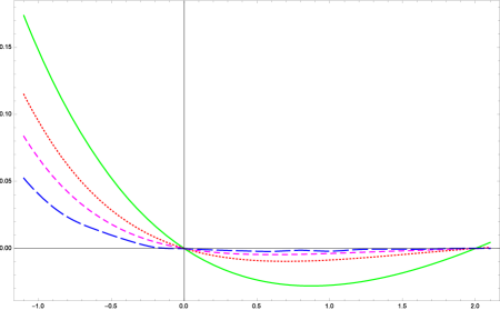
Figure 1: The graphs of the ratios $v_{4,0}^{\epsilon}/v_{00}^{\epsilon}$ (green, solid), $v_{6,6}^{\epsilon}/v_{00}^{\epsilon}$ (red, dotted), $v_{8,0}^{\epsilon}/v_{00}^{\epsilon}$ (magenta, short dashes) and $v_{12,0}^{\epsilon}/v_{00}^{\epsilon}$ (blue, long dashes) (listed in the decreasing order) as functions of the power $\epsilon$ in the potential Eq. (25). One can see the tendency of the higher-order coefficients to diminish with increasing value of index ${\rm K}$.

III.6 The Logarithmic potential

The logarithmic potential

$$V_{\rm Log}=\sigma_{\rm Log}\sum_{i>j=1}^{3}\log(|{\bf x}_{i}-{\bf x}_{j}|).$$ (26)

has a divergent short-distance and a steadily rising long-distance part; thence it can be thought of as a linear combination of the QCD Coulomb (with a homogeneity index $\alpha=-1$) and a linear confining potential (with a homogeneity index $\alpha=1$), with a common homogeneity index equal to zero: $\alpha=0$. Note that this homogeneity condition boils down to an additive, rather than multiplicative factorization of the potential:

$$V_{\rm Log}(R,\alpha,\phi) = V_{\rm Log}(R)+V_{\rm Log}(\alpha,\phi)$$ (27)

$$= V_{\rm Log}(R)+\sum_{K,{Q}}^{\infty}v_{K,{Q}}^{\rm Log}{\cal Y}^{K{Q}{\nu}}_{00}(\alpha,\phi)\$$

The logarithmic potential has been used with great success in the heavy-quark-antiquark two-body problem: it reproduces the remarkable mass-independence of the $c{\bar{c}}-J/\Psi$ and $b{\bar{b}}-\Upsilon$ spectra. It has not been used in the three-quark problem at all, to our knowledge.

Table 1: Expansion coefficients $v_{KQ}$ of the Y- and $\Delta$-string as well as of the Coulomb and Logarithmic potentials in terms of O(6) hyper-spherical harmonics ${\cal Y}_{0,0}^{K,0,0}$, for $K$ = 0, 4, 8, 12, respectively, and of the hyper-spherical harmonics ${\cal Y}_{0,0}^{6,\pm 6,0}$.

$(K,Q)$	$v_{KQ}({\rm Y-central})$	$v_{KQ}({\rm Y-string})$	$v_{KQ}(\Delta)$	$v_{KQ}({\rm Coulomb})$	$v_{KQ}(\rm Log)$
(0,0)	8.18	8.22	16.04	20.04	-6.58
(4,0)	-0.443	-0.398	- 0.445	2.93	-1.21
(6,$\pm$6)	0	-0.027	- 0.14	1.88	-0.56
(8,0)	- 0.064	-0.064	- 0.04	1.41	-0.33
(12,0)	-0.01	-0.01	0	0	-0.17

IV Results

In the following we present the ${\rm K}=0,\cdots,5$ shells’ energy spectra, for two reasons: (1) both as an example of the kind of results that one may expect as ${\rm K}$ increases, and in order to settle some long-standing issues regarding the ${\rm K}=3$ shell, Bowler:1981xh ; Bowler:1982ck ; Richard:1989ra ; (2) as an illustration of the methods, see Appendix B, that were used in their calculation. With regard to (2), we note that these examples are all purely algebraic, in the sense that no numerical calculations were necessary, but that ceases to be the case as ${\rm K}$ increases beyond ${\rm K}>8$, at first only for certain subsets of states, and ultimately, for all states.

We note that we have already reported at a conference Salom:2016prag , some of the ${\rm K}=4$ shell results, albeit without derivation.

IV.1 ${\rm K}=0,1,2$ shells

The ${\rm K}=0,1$ bands are affected only by the $v_{00}$ coefficient, so, they need not be treated separately here, whereas the ${\rm K}=2$ band is affected by the $v_{00}$ and $v_{40}$ coefficients. The calculated energy splittings of ${\rm K}=2$ shell states depend only on the SU(6) multiplets,

$$\left[20,1^{+}\right] \frac{1}{\pi\sqrt{\pi}}\Bigg{(} v_{00}-\frac{1}{\sqrt{3}}v_{40}\Bigg{)}$$

$$\left[70,0^{+}\right] \frac{1}{\pi\sqrt{\pi}}\Bigg{(} v_{00}+\frac{1}{\sqrt{3}}v_{40}\Bigg{)}$$

$$\left[70,2^{+}\right] \frac{1}{\pi\sqrt{\pi}}\Bigg{(} v_{00}-\frac{1}{5\sqrt{3}}v_{40}\Bigg{)}$$

$$\left[56,2^{+}\right] \frac{1}{\pi\sqrt{\pi}}\Bigg{(} v_{00}+\frac{\sqrt{3}}{5}v_{40}\Bigg{)},\$$ (28)

and the resulting spectrum is shown in Fig. 2.

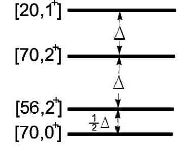
Figure 2: The K=2 spectrum of both the Y- and $\Delta$ strings in three dimensions.

Our main concern is the energy splitting pattern among the states within the K=2 hyper-spherical O(6) multiplet. The hyper-radial matrix elements of the linear hyper-radial potential are identical for all the (hyper-radial ground) states in one K band. Therefore, as is well known, the energy differences among various sub-states of a particular K band multiplet are integer multiples of the energy splitting “unit” $\Delta_{K}=\frac{1}{\pi\sqrt{\pi}}\Bigg{(}\frac{1}{5\sqrt{3}}-\frac{1}{\sqrt{3}}\Bigg{)}v_{40}=-\frac{1}{\pi\sqrt{\pi}}\frac{4}{5\sqrt{3}}v_{40}$. Note, however, that this kind of spectrum is subject to the condition $v_{00}\neq 0$.

IV.2 ${\rm K}=3$ shell

With only an area-dependent (i.e. $\phi$-independent) the central Y-string potential $V_{\rm Y-central}$, Eq. (9), in 3D, we find that the K=3 band $SU(6)$, or $S_{3}$ multiplets have one of four possible energies shown in Eqs. (29) with $v_{6\pm 6}^{\rm Y-central}=0$.

Upon introduction of the $\phi$-dependent two-body “V-string” potentials $V_{\rm V-string}$, Eqs. (32d)-(32k) into the full Y-string, the $v_{6\pm 6}^{\rm Y-string}$ coefficient becomes $\neq 0$. After diagonalization of the $C_{[K^{\prime}],[K]}$ matrix, one finds further splittings among the previously degenerate states $[70,1^{-}]$, $[56,3^{-}]$ and $[20,3^{-}]$, as well as among the $[70,3^{-}]$, $[56,1^{-}]$ and $[20,1^{-}]$:

$$\left[20,1^{-}\right] \frac{1}{\pi\sqrt{\pi}}\Bigg{(} v_{00}+\frac{1}{\sqrt{3}}v_{40}-\frac{2}{7}v_{66}\Bigg{)}$$

$$\left[56,1^{-}\right] \frac{1}{\pi\sqrt{\pi}}\Bigg{(} v_{00}+\frac{1}{\sqrt{3}}v_{40}+\frac{2}{7}v_{66}\Bigg{)}$$

$$\left[70,1^{-}\right] \frac{1}{\pi\sqrt{\pi}}\Bigg{(} v_{00}~{}~{}~{}~{}~{}~{}~{}~{}~{}~{}~{}~{}~{}~{}~{}~{}~{}~{}~{}~{}~{}~{}~{}\Bigg{)}$$

$$\left[70,2^{-}\right] \frac{1}{\pi\sqrt{\pi}}\Bigg{(} v_{00}-\frac{1}{\sqrt{3}}v_{40}~{}~{}~{}~{}~{}~{}~{}~{}~{}~{}\Bigg{)}$$

$$\left[70,3^{-}\right] \frac{1}{\pi\sqrt{\pi}}\Bigg{(} v_{00}-\frac{1}{\sqrt{3}}v_{40}~{}~{}~{}~{}~{}~{}~{}~{}~{}~{}\Bigg{)}$$

$$\left[20,3^{-}\right] \frac{1}{\pi\sqrt{\pi}}\Bigg{(} v_{00}-\frac{\sqrt{3}}{7}v_{40}~{}-~{}~{}v_{66}\Bigg{)}$$

$$\left[56,3^{-}\right] \frac{1}{\pi\sqrt{\pi}}\Bigg{(} v_{00}-\frac{\sqrt{3}}{7}v_{40}~{}+~{}~{}v_{66}\Bigg{)},\$$ (29)

where our $v_{66}<0$ is negative, and Richard and Taxil’s is positive. These results are displayed in Fig. 3.

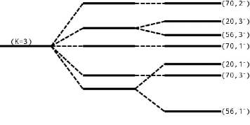
Figure 3: Schematic representation of the K=3 band in the energy spectrum of the $\Delta$-string potential in three dimensions, following Ref. Richard:1989ra . The sizes of the two splittings (the $v_{40}^{\rm\Delta}$-induced $\Delta$ and the subsequent $v_{6\pm 6}^{\rm\Delta}$-induced splitting) are not on the same scale, the latter having been increased, so as to be clearly visible. The $\Delta$ here is the same as the $\Delta$ in the K=2 band.

For the ${\rm K}=3$ band in 3D, the energy splittings have been calculated by Bowler and Tynemouth Bowler:1981xh , Bowler:1982ck for two-body anharmonic potentials perturbing the harmonic oscillator and confirmed and clarified by Richard and Taxil, Ref. Richard:1989ra , in the hyper-spherical formalism with linear two-body potentials (the $\Delta$-string).

In hindsight, Richard and Taxil’s Ref. Richard:1989ra separation of $V_{4}(R)$ and $V_{6}(R)$ potentials’ contributions is particularly illuminating: the former corresponds precisely to our “$\phi$-independent” term $v_{40}$ and the latter to the “$\phi$-dependent” potential’s contribution to $v_{66}$.

As both the central Y-string and the $\Delta$-string contain the former, whereas only the $\Delta$-string contains the latter, we see that the latter is the source of different degeneracies/splittings in the spectra of these two types of potentials.

IV.3 ${\rm K}=4$ shell

In the ${\rm K}=4$ band $SU(6)$, or $S_{3}$ multiplets have one of the following 12 values of the diagonalized $C$-matrix $C^{\rm K}_{{{[\rm m_{d}]}}}\times\frac{v_{00}}{\pi\sqrt{\pi}}$, from which one can evaluate the eigen-energies. We use the baryon-spectroscopic notation: $[{\rm dim.},L^{P}]$, where ${\rm dim.}$ is the dimension of the $SU_{\rm FS}(6)$ representation and the correspondence with the representations of the permutation group $S_{3}$ is given as $70\leftrightarrow M$, $20\leftrightarrow A$, $56\leftrightarrow S$.

$$\left[70,0^{+}\right]:\frac{1}{\pi\sqrt{\pi}}\Bigg{(}v_{00}+\frac{\sqrt{3}}{2}v_{40}+\frac{1}{2\sqrt{5}}v_{80}\Bigg{)}$$

$$\left[56,0^{+}\right]:\frac{1}{\pi\sqrt{\pi}}\Bigg{(}v_{00}~{}~{}~{}~{}~{}~{}~{}~{}~{}~{}~{}~{}~{}~{}+\frac{2}{\sqrt{5}}v_{80}\Bigg{)}$$

$$\left[70,1^{+}\right]:\frac{1}{\pi\sqrt{\pi}}\Bigg{(}v_{00}~{}~{}~{}~{}~{}~{}~{}~{}~{}~{}~{}~{}~{}~{}-\frac{1}{\sqrt{5}}v_{80}\Bigg{)}$$

$$\left[70,2^{+}\right]:\frac{1}{\pi\sqrt{\pi}}\Bigg{(}v_{00}+\frac{1}{35}\Big{(}7\sqrt{3}v_{40}+2\sqrt{5}v_{80}$$

$$-3\sqrt{3v_{40}^{2}-2\sqrt{15}v_{40}v_{80}+5v_{80}^{2}+120v_{6\pm 6}^{2}}\Big{)}\Bigg{)}$$

$$\left[70^{{}^{\prime}},2^{+}\right]:\frac{1}{\pi\sqrt{\pi}}\Bigg{(}v_{00}+\frac{1}{35}\Big{(}7\sqrt{3}v_{40}+2\sqrt{5}v_{80}$$

$$+3\sqrt{3v_{40}^{2}-2\sqrt{15}v_{40}v_{80}+5v_{80}^{2}+120v_{6\pm 6}^{2}}\Big{)}\Bigg{)}$$

$$\left[56,2^{+}\right]:\frac{1}{\pi\sqrt{\pi}}\Bigg{(}v_{00}-\frac{12\sqrt{3}}{35}v_{40}+\frac{\sqrt{5}}{7}v_{80}\Bigg{)}\$$

$$\left[20,2^{+}\right]:\frac{1}{\pi\sqrt{\pi}}\Bigg{(}v_{00}~{}~{}~{}~{}~{}~{}~{}~{}~{}~{}~{}~{}~{}~{}~{}-\frac{1}{\sqrt{5}}v_{80}\Bigg{)}$$

$$\left[20,3^{+}\right]:\frac{1}{\pi\sqrt{\pi}}\Bigg{(}v_{00}-\frac{3\sqrt{3}}{14}v_{40}-\frac{\sqrt{5}}{14}v_{80}\Bigg{)}$$

$$\left[70,3^{+}\right]:\frac{1}{\pi\sqrt{\pi}}\Bigg{(}v_{00}-\frac{5\sqrt{3}}{14}v_{40}+\frac{1}{14\sqrt{5}}v_{80}\Bigg{)}$$

$$\left[56,4^{+}\right]:\frac{1}{\pi\sqrt{\pi}}\Bigg{(}v_{00}+\frac{5\sqrt{3}}{14}v_{40}+\frac{3}{14\sqrt{5}}v_{80}\Bigg{)}$$

$$\left[70,4^{+}\right]:\frac{1}{\pi\sqrt{\pi}}\Bigg{(}v_{00}+\frac{1}{42\sqrt{5}}\Big{(}-2v_{80}$$

$$-\sqrt{1215v_{40}^{2}-54\sqrt{15}v_{40}v_{80}+9v_{80}^{2}+1280v_{6\pm 6}^{2}}\Big{)}\Bigg{)}$$

$$\left[70^{{}^{\prime}},4^{+}\right]:\frac{1}{\pi\sqrt{\pi}}\Bigg{(}v_{00}+\frac{1}{42\sqrt{5}}\Big{(}-2v_{80}$$

$$+\sqrt{1215v_{40}^{2}-54\sqrt{15}v_{40}v_{80}+9v_{80}^{2}+1280v_{6\pm 6}^{2}}\Big{)}\Bigg{)}.\$$ (30)

The $\Delta$-string results are shown in Fig. 4. Again, as the third coefficient $v_{6\pm 6}$ vanishes in the central Y-string potential $V_{\rm Y-central}$ (which is without two-body terms), or as it is roughly ten times smaller than usual, in the full Y-string potential $V_{\rm Y-string}$, the (second) observable difference between Y-string and $\Delta$-string potentials shows up in the magnitude of splitting between the pairs of $[70,2^{+}],[70^{{}^{\prime}},2^{+}]$ and $[70,4^{+}],[70^{{}^{\prime}},4^{+}]$ levels: the Y-string states are ordered as shown in the third ($v_{6\pm 6}=0$) column in Fig. 4. As explained earlier, the vanishing of $v_{6\pm 6}$ follows from the central Y-string potential’s independence of the Iwai angle $\phi$, i.e., from the dynamical “kinematic rotations/democracy transformations” O(2) symmetry, Dmitrasinovic:2009ma ; Dmitrasinovic:2014 associated with it.

Numerical results for other potentials are shown in Table 2.

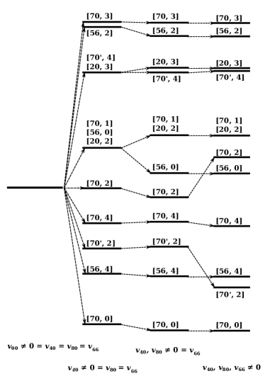
Figure 4: Schematic representation of the K=4 band in the energy spectrum of three quarks in the $\Delta$-string potential.

Table 2 shows that the ordering of K = 4 states is not universally valid even for the (convex) potentials considered here: note that although the three highest-lying multiplets always come from the same set ($[70,3^{+}],[56,2^{+}],[20,3^{+}],[70^{{}^{\prime}},4^{+}]$, see Fig. 4), their orderings are different in these potentials. That, of course, is a consequence of different ratios $v_{40}/v_{00}$, $v_{6\pm 6}/v_{00}$ and $v_{80}/v_{00}$. This goes to show that one cannot expect strongly restrictive ordering theorems to hold for three-body systems, as they hold in the two-body problem, Ref. Grosse:1997xu . Nevertheless, even the present results are useful, as they indicate that certain sets of multiplets are jointly lifted, or depressed, as a single group in the spectrum, with ordering within the group being subject to the detailed structure of the potential.

Of course, similar conclusions hold also for K = 3 spectrum splitting, but are less pronounced, as that shell depends only on two numbers: the ratios $v_{40}/v_{00}$ and $v_{6\pm 6}/v_{00}$. As the difference between $\Delta$ and Y-string potentials is most pronounced in the value of $v_{6\pm 6}$, that is the case where the distinction between these two potentials is most clearly seen.

Table 2: The values of effective potentials in the Y-, $\Delta$-string, and (strong) Coulomb potentials for various K = 4 states (for all allowed orbital waves L).

K	$[SU(6),L^{P}]$	$\langle\,{\rm V}_{\rm Y}/\sigma_{\rm Y}\,\rangle$	$\langle\,{\rm V}_{\Delta}/\sigma_{\Delta}\,\rangle$	$-\langle\,{\rm V}_{\rm C}/\alpha_{\rm C}\,\rangle$
4	$[56,0^{+}]$	1.45921	2.87122	3.82554
4	$[70,0^{+}]$	1.39729	2.80996	4.11043
4	$[70,1^{+}]$	1.47483	2.88587	3.48449
4	$[56,2^{+}]$	1.51372	2.92453	3.36709
4	$[20,2^{+}]$	1.47483	2.88587	3.48449
4	$[70,2^{+}]$	1.44997	2.87749	4.13184
4	$[70^{{}^{\prime}},2^{+}]$	1.43052	2.82683	3.49379
4	$[70,3^{+}]$	1.51906	2.92963	3.281
4	$[20,3^{+}]$	1.50137	2.91213	3.36239
4	$[56,4^{+}]$	1.4187	2.83095	3.94783
4	$[70,4^{+}]$	1.44036	2.85066	3.3656
4	$[70^{{}^{\prime}},4^{+}]$	1.49938	2.91178	3.81992

On the phenomenological side, some eigen-energies of three quarks in the ${\rm K}=4$ shell have been calculated in Ref. Stassart:1997vk using a variational method based on harmonic oscillator wave functions. These calculations included the $\Delta$-string, Y-string and Coulomb potentials, all at once, as well as a relativistic kinetic energy (this kinetic energy violates the O(6) symmetry). Each one of these three terms in the potential is homogenous, but their sum is not - therefore the individual contributions of these terms to the total/potential energy cannot be compared directly with the results of their separate calculations. Moreover, each term in the Hamiltonian breaks the O(6) symmetry differently, thus inducing different splittings of energy spectra. These facts prevent us from directly comparing our results with Ref. Stassart:1997vk , but the overall trend for groups of states seem to be in agreement with our results, see Table 2, for comparison.

IV.4 ${\rm K}=5$ shell

With a $\phi$-independent central Y-string potential in 3D, we find that the ${\rm K}=5$ band $SU(6)$, or $S_{3}$ multiplets have one of 15 different energies. Upon introduction of a $\phi$-dependent (“two-body”) component of the potential, proportional to $v_{66}$,and upon diagonalization of the $C_{[K^{\prime}],[K]}$ matrix, one finds four new splittings between previously degenerate states 1) $[56,2^{-}],[20,2^{-}]$, 2) $[56^{{}^{\prime}},4^{-}],[20^{{}^{\prime}},4^{-}]$, 3) $[70~{},1^{-}],[70^{{}^{\prime}},1^{-}]$, 4) $[70~{},5^{-}],[70^{{}^{\prime}},5^{-}]$, as well as three non-degenerate states whose energies are shifted by $v_{66}$. These algebraic results are summarized in

$$\left[70,1^{-}\right] \frac{1}{\pi\sqrt{\pi}}\Bigg{(} v_{00}+\frac{5\sqrt{3}v_{40}+3\sqrt{5}v_{80}}{20}$$

$$- \frac{\sqrt{75v_{40}^{2}-10\sqrt{15}v_{40}v_{80}+5v_{80}^{2}+96v_{6\pm 6}^{2}}}{20}\Bigg{)}$$

$$\left[70^{{}^{\prime}},1^{-}\right] \frac{1}{\pi\sqrt{\pi}}\Bigg{(} v_{00}+\frac{5\sqrt{3}v_{40}+3\sqrt{5}v_{80}}{20}$$

$$+ \frac{\sqrt{75v_{40}^{2}-10\sqrt{15}v_{40}v_{80}+5v_{80}^{2}+96v_{6\pm 6}^{2}}}{20}\Bigg{)}$$

$$\left[56,1^{-}\right] \frac{1}{\pi\sqrt{\pi}}\Bigg{(} v_{00}+\frac{1}{2\sqrt{3}}v_{40}-\frac{2}{5}v_{66}-\frac{1}{2\sqrt{5}}v_{80}\Bigg{)}$$

$$\left[20,1^{-}\right] \frac{1}{\pi\sqrt{\pi}}\Bigg{(} v_{00}+\frac{1}{2\sqrt{3}}v_{40}+\frac{2}{5}v_{66}-\frac{1}{2\sqrt{5}}v_{80}\Bigg{)}$$

$$\left[70,2^{-}\right] \frac{1}{\pi\sqrt{\pi}}\Bigg{(} v_{00}-\frac{1}{2\sqrt{3}}v_{40}~{}~{}~{}~{}~{}~{}~{}~{}~{}~{}-\frac{1}{2\sqrt{5}}v_{80}\Bigg{)}$$

$$\left[56,2^{-}\right] \frac{1}{\pi\sqrt{\pi}}\Bigg{(} v_{00}~{}~{}~{}~{}~{}~{}~{}~{}~{}~{}~{}~{}~{}~{}+\frac{3}{5}v_{66}-\frac{1}{\sqrt{5}}v_{80}\Bigg{)}$$

$$\left[20,2^{-}\right] \frac{1}{\pi\sqrt{\pi}}\Bigg{(} v_{00}~{}~{}~{}~{}~{}~{}~{}~{}~{}~{}~{}~{}~{}~{}-\frac{3}{5}v_{66}-\frac{1}{\sqrt{5}}v_{80}\Bigg{)}\$$

$$\left[56,3^{-}\right] \frac{1}{\pi\sqrt{\pi}}\Bigg{(} v_{00}+\frac{1}{2\sqrt{3}}v_{40}+\frac{14}{15}v_{66}+\frac{7}{6\sqrt{5}}v_{80}\Bigg{)}$$

$$\left[20,3^{-}\right] \frac{1}{\pi\sqrt{\pi}}\Bigg{(} v_{00}+\frac{1}{2\sqrt{3}}v_{40}-\frac{14}{15}v_{66}+\frac{7}{6\sqrt{5}}v_{80}\Bigg{)}$$

$$\left[70,4^{-}\right] \frac{1}{\pi\sqrt{\pi}}\Bigg{(} v_{00}-\frac{1}{2\sqrt{3}}v_{40}~{}~{}~{}~{}~{}~{}~{}~{}~{}~{}~{}~{}-\frac{1}{2\sqrt{5}}v_{80}\Bigg{)}$$

$$\left[56,4^{-}\right] \frac{1}{\pi\sqrt{\pi}}\Bigg{(} v_{00}-\frac{7}{6\sqrt{3}}v_{40}-\frac{2}{15}v_{66}+\frac{1}{6\sqrt{5}}v_{80}\Bigg{)}$$

$$\left[20,4^{-}\right] \frac{1}{\pi\sqrt{\pi}}\Bigg{(} v_{00}-\frac{7}{6\sqrt{3}}v_{40}+\frac{2}{15}v_{66}+\frac{1}{6\sqrt{5}}v_{80}\Bigg{)}$$

$$\left[70,5^{-}\right] \frac{1}{\pi\sqrt{\pi}}\Bigg{(} v_{00}+\frac{\sqrt{3}}{18}v_{40}+\frac{\sqrt{5}}{30}v_{80}$$

$$+ \frac{\sqrt{5}}{165} \sqrt{1815v_{40}^{2}+66\sqrt{15}v_{40}v_{80}+9v_{80}^{2}+968v_{6\pm 6}^{2}}\Bigg{)}$$

$$\left[70^{{}^{\prime}},5^{-}\right] \frac{1}{\pi\sqrt{\pi}}\Bigg{(} v_{00}+\frac{\sqrt{3}}{18}v_{40}+\frac{\sqrt{5}}{30}v_{80}$$

$$-\frac{\sqrt{5}}{165} \sqrt{1815v_{40}^{2}+66\sqrt{15}v_{40}v_{80}+9v_{80}^{2}+968v_{6\pm 6}^{2}}\Bigg{)}$$

$$\left[56,5^{-}\right] \frac{1}{\pi\sqrt{\pi}}\Bigg{(} v_{00}+\frac{1}{2\sqrt{3}}v_{40}+\frac{8}{15}v_{66}-\frac{19}{66\sqrt{5}}v_{80}\Bigg{)}$$

$$\left[20,5^{-}\right] \frac{1}{\pi\sqrt{\pi}}\Bigg{(} v_{00}+\frac{1}{2\sqrt{3}}v_{40}-\frac{8}{15}v_{66}-\frac{19}{66\sqrt{5}}v_{80}\Bigg{)}\$$ (31)

The numerical results are displayed in Table 3 for different potentials, and in Table 4 for the $\Delta$-string potential it has been broken up into contributions of different multipoles of the potential and are graphically displayed in Fig. 5.

Table 3: The values of the effective potential matrix elements for the Y-, $\Delta$-string, and (strong) Coulomb potential, and various K = 5 states (for all allowed orbital waves L).

K	$[SU(6),L^{P}]$	$\langle\,{\rm V}_{\rm Y}/\sigma_{\rm Y}\,\rangle$	$\langle\,{\rm V}_{\Delta}/\sigma_{\Delta}\,\rangle$	$-\langle\,{\rm V}_{\rm C}/\alpha_{\rm C}\,\rangle$
5	$[70,1^{-}]$	1.39729	2.80778	2.55667
5	$[70^{{}^{\prime}},1^{-}]$	1.46442	2.87829	2.85542
5	$[56,1^{-}]$	1.44898	2.87055	2.46858
5	$[20,1^{-}]$	1.44898	2.85059	2.5953
5	$[70,2^{-}]$	1.49547	2.90629	2.32887
5	$[20,2^{-}]$	1.47483	2.87091	2.47611
5	$[56,2^{-}]$	1.47483	2.90084	2.28602
5	$[70,3^{-}]$	1.46682	2.84167	2.41462
5	$[70^{{}^{\prime}},3^{-}]$	1.44037	2.8887	2.30016
5	$[70^{{}^{\prime\prime}},3^{-}]$	1.5103	2.92104	2.67414
5	$[56,3^{-}]$	1.44031	2.82915	2.84424
5	$[20,3^{-}]$	1.44031	2.87571	2.54855
5	$[70,4^{-}]$	1.49547	2.90629	2.32887
5	$[56,4^{-}]$	1.52299	2.93685	2.23815
5	$[20,4^{-}]$	1.52299	2.93020	2.28039
5	$[70,5^{-}]$	1.50797	2.91991	2.75234
5	$[70^{{}^{\prime}},5^{-}]$	1.41405	2.82520	2.30772
5	$[56,5^{-}]$	1.44788	2.84623	2.63735
5	$[20,5^{-}]$	1.44788	2.87283	2.46839

Table 4: The values of the effective three-body $\Delta$-string potential divided by the string tension $\sigma_{\Delta}$, $\langle\,{\rm V}_{\Delta}(v_{0,0},v_{4,0},v_{6,6},v_{8,0})/\sigma_{\Delta}\,\rangle$ as a function of the expansion coefficients $(v_{0,0},v_{4,0},v_{6,6},v_{8,0})$, for various ${\rm K}=5$ states (for all allowed orbital waves $L$). Here $\langle\,{\rm V}_{\Delta}(A)/\sigma_{\Delta}\,\rangle=\langle\,{\rm V}_{\Delta}(v_{0,0},v_{4,0}\neq 0=v_{6,6}=v_{8,0})/\sigma_{\Delta}\,\rangle$ and $\langle\,{\rm V}_{\Delta}(B)/\sigma_{\Delta}\,\rangle=\langle\,{\rm V}_{\Delta}(v_{0,0},v_{4,0},v_{8,0}\neq 0=v_{6,6})/\sigma_{\Delta}\,\rangle$

K	$[SU(6),L^{P}]$	$\langle\,{\rm V}_{\Delta}(A)/\sigma_{\Delta}\,\rangle$	$\langle\,{\rm V}_{\Delta}(B)/\sigma_{\Delta}\,\rangle$	$\langle\,{\rm V}_{\Delta}/\sigma_{\Delta}\,\rangle$
5	$[70,1^{-}]$	2.8124	2.80996	2.80778
5	$[70^{{}^{\prime}},1^{-}]$	2.88099	2.87611	2.87829
5	$[56,1^{-}]$	2.85813	2.86057	2.87055
5	$[20,1^{-}]$	2.85813	2.86057	2.85059
5	$[70,2^{-}]$	2.90385	2.90629	2.90629
5	$[56,2^{-}]$	2.88099	2.88587	2.87091
5	$[20,2^{-}]$	2.88099	2.88587	2.90084
5	$[70,3^{-}]$	2.85051	2.85214	2.84167
5	$[70^{{}^{\prime}},3^{-}]$	2.87918	2.87827	2.8887
5	$[70^{{}^{\prime\prime}},3^{-}]$	2.92091	2.921	2.92104
5	$[56,3^{-}]$	2.85813	2.85243	2.82915
5	$[20,3^{-}]$	2.85813	2.85243	2.87571
5	$[70,4^{-}]$	2.90385	2.90629	2.90629
5	$[56,4^{-}]$	2.93434	2.93352	2.93685
5	$[20,4^{-}]$	2.93434	2.93352	2.93020
5	$[70,5^{-}]$	2.91909	2.91872	2.91991
5	$[70^{{}^{\prime}},5^{-}]$	2.82764	2.82639	2.82520
5	$[56,5^{-}]$	2.85813	2.85953	2.84623
5	$[20,5^{-}]$	2.85813	2.85953	2.87283

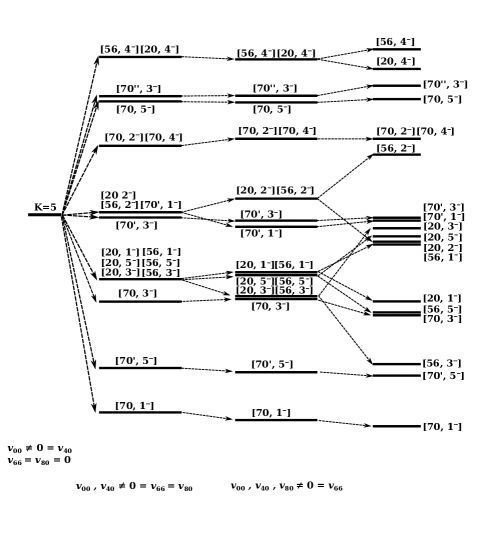
Figure 5: Schematic representation of the K=5 band in the energy spectrum of the $\Delta$- and Y-string potentials in three dimensions. The sizes of the two splittings (the $v_{40}^{\rm\Delta}$-induced $\Delta$ and the subsequent $v_{80}^{\rm\Delta}$-induced splitting) are not on the same scale. The $\Delta$ here is not the same as the $\Delta$ in the K=2 band.

V Discussion and comparison with previous calculations

1) The present results are meant (only) as examples of what can be done: these calculations can be extended with ${\rm K}$ increasing ad infinitum, with the help of O(6) matrix elements that are functions of O(6) Clebsch-Gordan coefficients, which can be found in Ref. Salom:2017ekb . This is subject to the proviso that at some value of ${\rm K}$ the calculations must necessarily become numerical.

2) The algebraic results shown in Sect. IV do not hold for the QCD Coulomb potential, as the QCD Coulomb hyper-radial potential $-\alpha_{C}/R$ Eq. (III.3) has a dynamical O(7) symmetry and therefore accidental degeneracies are expected to appear. That symmetry is broken by the hyper-angular part of the Coulomb three-body potential in a manner that still remains to be explored.

3) In the ${\rm K}=2$ band/shell of the three-body energy spectrum the eigen-energies depend on two coefficients $(v_{00},v_{40})$, and the splittings among various levels depend only on the (generally small) ratio $v_{40}/v_{00}$. This means that the eigen-energies form a fixed pattern (“ordering”) that does not depend on the shape of the three-body potential. The actual size of the ${\rm K}=2$ shell energy splitting depends on the small parameter $v_{40}/v_{00}$, provided that the potential is permutation symmetric. This fact was noticed almost 40 years ago, Refs. Gromes:1976cr ; Isgur:1978wd , and it suggested that similar patterns might exist in higher-${\rm K}$ shells.

The practical advantage of permutation-adapted hyperspherical harmonics over the conventional ones is perhaps best illustrated here: the ${\rm K}=2$ shell splittings in the Y- and $\Delta$-string potentials were obtained, after some complicated calculations using conventional hyperspherical harmonics in Ref. Dmitrasinovic:2009dy , whereas here they follow from the calculation of four (simple) hyper-angular matrix elements.

4) Historically, extensions of this kind of calculations to higher (${\rm K}\geq 3$) bands, for general three-body potentials turned out more problematic than expected: Bowler et. al, Ref. Bowler:1981xh , published a set of predictions for the ${\rm K}=3,4$ bands, which were later questioned by Richard and Taxil’s ${\rm K}=3$ hyperspherical harmonic calculation, Ref. Richard:1989ra ; see also Refs. Stancu:1991cz ; Stassart:1997vk . This controversy had not been resolved up to the present day, to our knowledge, so we address that problem first: In the ${\rm K}=3$ case the energies depend on three coefficients $(v_{00},v_{40},v_{6\pm 6})$, and there is no mixing of multiplets, so all eigen-energies can be expressed in simple closed form that agrees with Ref. Richard:1989ra and depends on two small parameters $v_{40}/v_{00},v_{6\pm 6}/v_{00}$.

Note that the coefficient $v_{6\pm 6}$ vanishes in the (simplified) central Y-string potential (without two-body terms) and thus causes the first potentially observable difference betwen Y- and $\Delta$-string potentials: the splittings between $\left[20,1^{-}\right]$, and $\left[56,1^{-}\right]$, as well as between $\left[20,3^{-}\right]$, and $\left[56,3^{-}\right]$. The actual value of $v_{6\pm 6}$ in the exact Y-string potential is so small, as to be negligible compared with the other two coefficients, $v_{00},v_{40}$, in its expansion.

5) Note that from Eq. (7) it follows that there must exist an upper limit on the values of the ratios $|v_{40}/v_{00}|\leq\sqrt{3}$, and from Eq. (8) it follows $|v_{6\pm 6}/v_{00}|\leq 7/2$. If these limits are exceeded, the overall sign of the effective potential flips, and the solution (motion) becomes unbound. This example clearly shows the limitations of the present method. However, the physically interesting potentials considered in Sect. III all satisfy inequalities $v_{00}\gg|v_{40}|$, and $v_{00}\gg|v_{6\pm 6}|$, as can be seen in Table 1 and Fig. 1, which shows that this method may be applied here.

6) The above points (2) and (3) display possible “fault line(s)” in the predictions of ordering of shells with different values of ${\rm K}$: in case $v_{00}=0$, the ${\rm K}=0,1$ shells become unbound to leading (adiabatic) order, and their binding becomes a question of higher-order (non-adiabatic) effects.

7) We shall not attempt a numerical predictions of triple-heavy hyperon masses here, for the following reasons: (a) the mass of heavy quark(s) $m_{Q}$ is not precisely known in the three-quark environment; (b) the QCD coupling constant $\alpha_{S}$ is not known in this environment; (c) the value of the effective string tension $\sigma$ is not known in this environment; (d) the spin-dependent interactions, which are not included here, may significantly influence the results. Nevertheless, nothing prevents the interested reader from inserting his/her favourite values of $m_{Q}$, $\alpha_{S}$ and $\sigma$ into our formulae to obtain some definite predictions.

8) There are several possible straightforward extensions of the present work: (a) to equal mass systems with a relativistic kinematic energy; (b) to two identical and one distinct quark systems. Both extensions break the O(6) symmetry further still, but can be treated within the present approach, with certain caveats.

9) Note that we have kept the full $SU_{F}(3)$, $SU_{FS}(6)$ notation for the three-quark states, even though there can be only one flavour, with three identical heavy quarks. This is in order to keep maximum generality, and to allow potential future extension to relativistic light quark systems (c.f. Stancu:1991cz ; Stassart:1997vk ).

10) The present formalism allows a (mathematically proper) extension of the Regge theory/trajectories Regge:1959 to three-quark systems, as well as an extension of Birman-Schwinger’s results Birman:1961 ; Schwinger:1961 about the number of bound states of a Schrödinger equation in a given potential.

11) The present formalism allows an extension to atomic and molecular physics, as well, albeit with significant modifications: (a) atomic systems are subject to Coulomb potential, which leads to a higher dynamical symmetry, that needs to be taken into account; and (b) molecular systems are bound by inhomogenous potentials, such as the Lennard-Jones one, which must be treated differently.

VI Summary and Conclusions

In summary, we have reduced the non-relativistic (quantum) three-identical-body problem to a single ordinary differential equation for the hyper-radial wave function with coefficients multiplying the homogenous hyper-radial potential that are determined entirely by O(6) group-theoretical arguments, see Salom:2016vcw ; Salom:2017ekb . That equation can be solved in the same way as the radial Schrödinger equation in 3D. The breaking of the O(6) symmetry by the three-quark potential determines the ordering of states within different shells in the energy spectrum.

The dynamical $O(2)$ symmetry of the Y-string potential was discovered in Ref. Dmitrasinovic:2009ma , with the permutation group $S_{3}\subset O(2)$ as the subgroup of the dynamical $O(2)$ symmetry. The existence of an additional dynamical symmetry strongly suggested an algebraic approach, such as that used in two-dimensional space, in Ref. Dmitrasinovic:2014 . In three dimensions (3D) the hyper-spherical symmetry group is O(6), and the residual dynamical symmetry of the potential is $S_{3}\otimes SO(3)_{rot}\subset O(2)\otimes SO(3)_{rot}\subset O(6)$, where $SO(3)_{rot}$ is the rotational symmetry associated with the (total orbital) angular momentum $L$. We showed how the energy eigenvalues can be calculated as functions of the three-body potential’s (hyper-)spherical harmonics expansion coefficients $v_{{\rm K},{Q}}^{\rm 3-body}$ and O(6) Clebsch-Gordan coefficients that are evaluated in Ref. Salom:2017ekb .

We have used these results to calculate the energy splittings of various states (or $SU_{FS}(6)$ and $S_{3}$ multiplets) in the ${\rm K}\leq 5$ shells of the Y-, $\Delta$-string and Coulomb potential spectra. The ordering of bound states has its most immediate application in the physics of three confined quarks, where the question was raised originally, Refs. Gromes:1976cr ; Isgur:1978wd ; Bowler:1981xh ; Richard:1989ra . We have shown that in the ${\rm K}\geq 3$ shells a clear difference appears between the spectra of the Y- and $\Delta$-string models of confinement. That is also the first explicit consequence of the dynamical O(2) symmetry of the “Y-string” potential.

We stress the algebraic nature of our results, as this method can be used to obtain predictions for arbitrarily large ${\rm K}$ values, which calculations must necessarily be numerical, however, as soon as the number of states that are mixed exceeds five.

The results presented here do not represent the outer boundaries of applicability of our method, but are rather just illustrative examples, with a view to its application to atomic, molecular and nuclear physics.

Appendix A Evaluation of obtuse-angled two-body contributions to the Y-string

As stated in Sect. II at obtuse angles ($\geq 120^{0}$) there are two-body contributions to the Y-string potential that break the dynamical O(2) symmetry of Eq. (15). Therefore, the expansion coefficient $v_{{\rm K}=6,{Q}=\pm 6}^{\rm Y-string}$ of the full potential is not zero $v_{6,\pm 6}^{\rm Y-string}\neq 0$.

Three angle-dependent two-body string in terms of Jacobi vectors ${\bm{\rho}},{\bm{\lambda}}$ are, see Ref. Dmitrasinovic:2009dy ,

$$V_{\rm V-string} = \sigma\left(\sqrt{\frac{1}{2}({\bm{\rho}}^{2}+3{\bm{\lambda}}^{2}+2\sqrt{3}{\bm{\rho}}\cdot{\bm{\lambda}})}+\sqrt{\frac{1}{2}({\bm{\rho}}^{2}+3{\bm{\lambda}}^{2}-2\sqrt{3}{\bm{\rho}}\cdot{\bm{\lambda}})}\right)$$ (32d)

$$\textrm{when}\left\{\begin{array}[]{l}\quad 2{\bm{\rho}}^{2}-\sqrt{3}{\bm{\rho}}\cdot{\bm{\lambda}}\geq-\rho\sqrt{{\bm{\rho}}^{2}+3{\bm{\lambda}}^{2}-2\sqrt{3}{\bm{\rho}}\cdot{\bm{\lambda}}}\\ \quad 2{\bm{\rho}}^{2}+\sqrt{3}{\bm{\rho}}\cdot{\bm{\lambda}}\geq-\rho\sqrt{{\bm{\rho}}^{2}+3{\bm{\lambda}}^{2}+2\sqrt{3}{\bm{\rho}}\cdot{\bm{\lambda}}}\\ \quad 3{\bm{\lambda}}^{2}-{\bm{\rho}}^{2}\leq-\frac{1}{2}\sqrt{({\bm{\rho}}^{2}+3{\bm{\lambda}}^{2})^{2}-12({\bm{\rho}}\cdot{\bm{\lambda}})^{2}}\\ \end{array}\right.$$

$$V_{\rm V-string} = \sigma\left(\sqrt{2}\rho+\sqrt{\frac{1}{2}({\bm{\rho}}^{2}+3{\bm{\lambda}}^{2}+2\sqrt{3}{\bm{\rho}}\cdot{\bm{\lambda}})}\right)$$ (32g)

$$\textrm{when}\left\{\begin{array}[]{l}\quad 2{\bm{\rho}}^{2}-\sqrt{3}{\bm{\rho}}\cdot{\bm{\lambda}}\geq-\rho\sqrt{{\bm{\rho}}^{2}+3{\bm{\lambda}}^{2}-2\sqrt{3}{\bm{\rho}}\cdot{\bm{\lambda}}}\\ \quad 2{\bm{\rho}}^{2}+\sqrt{3}{\bm{\rho}}\cdot{\bm{\lambda}}\leq-\rho\sqrt{{\bm{\rho}}^{2}+3{\bm{\lambda}}^{2}+2\sqrt{3}{\bm{\rho}}\cdot{\bm{\lambda}}}\\ \quad 3{\bm{\lambda}}^{2}-{\bm{\rho}}^{2}\geq-\frac{1}{2}\sqrt{({\bm{\rho}}^{2}+3{\bm{\lambda}}^{2})^{2}-12({\bm{\rho}}\cdot{\bm{\lambda}})^{2}}\end{array}\right.$$

$$V_{\rm V-string} = \sigma\left(\sqrt{2}\rho+\sqrt{\frac{1}{2}({\bm{\rho}}^{2}+3{\bm{\lambda}}^{2}-2\sqrt{3}{\bm{\rho}}\cdot{\bm{\lambda}})}\right)$$ (32k)

$$\textrm{when}\left\{\begin{array}[]{l}\quad 2{\bm{\rho}}^{2}-\sqrt{3}{\bm{\rho}}\cdot{\bm{\lambda}}\leq-\rho\sqrt{{\bm{\rho}}^{2}+3{\bm{\lambda}}^{2}-2\sqrt{3}{\bm{\rho}}\cdot{\bm{\lambda}}}\\ \quad 2{\bm{\rho}}^{2}+\sqrt{3}{\bm{\rho}}\cdot{\bm{\lambda}}\geq-\rho\sqrt{{\bm{\rho}}^{2}+3{\bm{\lambda}}^{2}+2\sqrt{3}{\bm{\rho}}\cdot{\bm{\lambda}}}\\ \quad 3{\bm{\lambda}}^{2}-{\bm{\rho}}^{2}\geq-\frac{1}{2}\sqrt{({\bm{\rho}}^{2}+3{\bm{\lambda}}^{2})^{2}-12({\bm{\rho}}\cdot{\bm{\lambda}})^{2}}\end{array}\right.\,.$$

The O(6) $v_{6\pm 6}$ coefficient is defined in Eq. (4)

$$v_{6,\pm 6}^{\rm Y-string}=\int~{}{\cal Y}^{6\pm 6}_{00}(\Omega_{5})\,V_{\rm Y-string}(\alpha,\phi)\,\,d\Omega_{(5)}$$ (33)

where the integration over $d\Omega_{(5)}$ is constrained by inequalities (32d) - (32k) and

$${\mathcal{Y}}^{6,\pm 6}_{00}(\alpha,\phi) = \frac{2}{\pi^{3/2}}R^{-6}\left({\bm{\lambda}}^{2}-{\bm{\rho}}^{2}\pm 2i{\bm{\lambda}}\cdot{\bm{\rho}}\right)^{3}$$ (34)

$$= \frac{\mp 2i}{\pi^{3/2}}\sin^{3}\alpha\exp\left(\mp 3i\phi\right)\$$

which is equivalent, up to the normalization constant, to the O(3) spherical harmonics $Y_{3,\pm 3}\left(\alpha,\phi\right)$. Numerical evaluation yields $v_{6,\pm 6}^{\rm Y-string}=-0.027$, which value is smaller than the subsequent coefficients in the expansion of this potential, see Table 1.

Appendix B Details of calculations

B.1 ${\rm K}=2$ shell

The calculated coefficients entering the effective potentials for states with ${\rm K}=2$ can be found in Table 5.

Table 5: The values of the three-body potential hyper-angular matrix elements $\pi\sqrt{\pi}\langle\,{\mathcal{Y}}^{4,0}_{00}\,\rangle_{\rm ang}$, for various K = 2 states (for all allowed orbital waves L). The correspondence between the $S_{3}$ permutation group irreps. and SU(6)_FS symmetry multiplets of the three-quark system: $S\leftrightarrow 56$, $A\leftrightarrow 20$ and $M\leftrightarrow 70$.

K	$\left(K,Q,L,M,\nu\right)$	$[SU(6),L^{P}]$	$\pi\sqrt{\pi}\langle\,{\mathcal{Y}}^{4,0}_{00}\,\rangle_{\rm ang}$
2	$\left(2,-2,0,0,0\right)$	$[70,0^{+}]$	$\frac{1}{\sqrt{3}}$
2	$\left(2,~{}0,2,2,0\right)$	$[56,2^{+}]$	$\frac{\sqrt{3}}{5}$
2	$\left(2,\mp 2,2,2,\pm 3\right)$	$[70,2^{+}]$	$-\frac{1}{5\sqrt{3}}$
2	$\left(2,0,1,1,0\right)$	$[20,1^{+}]$	$-\frac{1}{\sqrt{3}}$

B.2 ${\rm K}=3$ shell

The calculated effective potentials in states with of K=3 and various values L are listed in Tables 6 and 7.

Table 6: The values of the three-body potential hyper-angular diagonal matrix elements $\langle\,{\mathcal{Y}}^{4,0}_{00}\,\rangle_{\rm ang}$, for various K = 3 states (for all allowed orbital waves L).

K	$\left(K,Q,L,M,\nu\right)$	$[SU(6),L^{P}]$	$\pi\sqrt{\pi}\langle\,{\cal Y}^{4,0}_{00}\,\rangle_{\rm ang}$
3	$\left(3,\mp 3,~{}1,~{}1,\pm 1\right)$	$[20,1^{-}]$	$~{}\frac{1}{\sqrt{3}}$
3	$\left(3,\mp 3,~{}1,~{}1,\pm 1\right)$	$[56,1^{-}]$	$~{}\frac{1}{\sqrt{3}}$
3	$\left(3,\pm 1,~{}1,~{}1,\pm 3\right)$	$[70,1^{-}]$	$~{}0$
3	$\left(3,\mp 1,~{}2,~{}2,\pm 5\right)$	$[70,2^{-}]$	$-\frac{1}{\sqrt{3}}$
3	$\left(3,\mp 1,~{}3,~{}3,\pm 2\right)$	$[70,3^{-}]$	$~{}\frac{5}{7\sqrt{3}}$
3	$\left(3,\pm 3,~{}3,~{}3,\mp 6\right)$	$[56,3^{-}]$	$-\frac{\sqrt{3}}{7}$
3	$\left(3,\pm 3,~{}3,~{}3,\mp 6\right)$	$[20,3^{-}]$	$-\frac{\sqrt{3}}{7}$

Table 7: The values of the off-diagonal matrix elements of the hyper-angular part of the three-body potential $\pi\sqrt{\pi}\langle[SU(6)_{f},L_{f}^{P}]|\,2\Re e\mathcal{Y}^{6,\pm 6,0}_{0,0}\,|[SU(6)_{i},L_{i}^{P}]\rangle_{\rm ang}$, for various K = 3 states (for all allowed orbital waves L).

K	$[SU(6)_{f},L_{f}^{P}]$	$[SU(6)_{i},L_{i}^{P}]$	$\pi\sqrt{\pi}\langle 2\Re e\mathcal{Y}^{6,\pm 6,0}_{0,0}\rangle_{\rm ang}$
3	$[20,1^{-}]$	$[20,1^{-}]$	$-1$
3	$[56,1^{-}]$	$[56,1^{-}]$	$~{}~{}1$
3	$[20,3^{-}]$	$[20,3^{-}]$	$-\frac{2}{7}$
3	$[56,3^{-}]$	$[56,3^{-}]$	$~{}~{}\frac{2}{7}$
3	$[70,L^{-}]$	$[70,L^{-}]$	$~{}~{}0$

B.3 ${\rm K}=4$ shell

The calculated effective potentials for states with K=4 and various values of L are listed in Table 8.

Table 8: The values of the three-body potential hyper-angular diagonal matrix elements $\langle\,{\mathcal{Y}}^{4,0,0}_{00}\,\rangle_{\rm ang}$ and $\langle\,{\mathcal{Y}}^{8,0,0}_{00}\,\rangle_{\rm ang}$, for various K = 4 states (for all allowed orbital waves L).

K	$\left(K,Q,L,M,\nu\right)$	$[SU(6),L^{P}]$	$\pi\sqrt{\pi}\langle\,{\mathcal{Y}}^{4,0,0}_{00}\,\rangle_{\rm ang}$	$\pi\sqrt{\pi}\langle\,{\mathcal{Y}}^{8,0,0}_{00}\,\rangle_{\rm ang}$
4	$\left(4,\pm 4,0,0,~{}~{}0\right)$	$[70,0^{+}]$	$~{}\frac{\sqrt{3}}{2}$	$~{}\frac{1}{2\sqrt{5}}$
4	$\left(4,~{}~{}0,0,0,~{}~{}0\right)$	$[56,0^{+}]$	$~{}0$	$~{}\frac{2}{\sqrt{5}}$
4	$\left(4,\pm 2,1,1,\pm 2\right)$	$[70,1^{+}]$	$~{}~{}0$	$-\frac{1}{\sqrt{5}}$
4	$\left(4,0,2,2,\mp\sqrt{105}\right)$	$[56,2^{+}]$	$-\frac{12\sqrt{3}}{35}$	$\frac{\sqrt{5}}{7}$
4	$\left(4,0,2,2,\mp\sqrt{105}\right)$	$[20,2^{+}]$	$0$	$-\frac{1}{\sqrt{5}}$
4	$\left(4,\pm 2,2,2,\pm 2\right)$	$[70,2^{+}]$	$\frac{4\sqrt{3}}{35}$	$\frac{\sqrt{5}}{7}$
4	$\left(4,\pm 4,2,2,\mp 3\right)$	$[70^{{}^{\prime}},2^{+}]$	$~{}\frac{2\sqrt{3}}{7}$	$-\frac{1}{7\sqrt{5}}$
4	$\left(4,\mp 2,3,3,\pm 13\right)$	$[70,3^{+}]$	$-\frac{5\sqrt{3}}{14}$	$~{}\frac{1}{14\sqrt{5}}$
4	$\left(4,~{}~{}0,3,3,~{}~{}0\right)$	$[20,3^{+}]$	$-\frac{3\sqrt{3}}{14}$	$-\frac{\sqrt{5}}{14}$
4	$\left(4,~{}~{}0,4,4,~{}~{}0\right)$	$[56,4^{+}]$	$\frac{5\sqrt{3}}{14}$	$~{}\frac{3}{14\sqrt{5}}$
4	$\left(4,\mp 2,4,4,\pm 5\right)$	$[70,4^{+}]$	$\frac{3\sqrt{3}}{14}$	$-\frac{\sqrt{5}}{42}$
4	$\left(4,\mp 4,4,4,\pm 10\right)$	$[70^{{}^{\prime}},4^{+}]$	$-\frac{3\sqrt{3}}{14}$	$\frac{1}{42\sqrt{5}}$

Table 9: The values of the off-diagonal matrix elements of the hyper-angular part of the three-body potential $\pi\sqrt{\pi}\langle[SU(6)_{f},L_{f}^{P}]|\,2\Re e\mathcal{Y}^{6,\pm 6,0}_{0,0}\,|[SU(6)_{i},L_{i}^{P}]\rangle_{\rm ang}$, for various K = 4 states (for all allowed orbital waves L).

K	$[SU(6)_{f},L_{f}^{P}]$	$[SU(6)_{i},L_{i}^{P}]$	$\pi\sqrt{\pi}\langle 2\Re e\mathcal{Y}^{6,\pm 6,0}_{0,0}\rangle_{\rm ang}$
4	$[70,2^{+}]$	$[70^{{}^{\prime}},2^{+}]$	$\frac{6}{7}\sqrt{\frac{6}{5}}$
4	$[70^{{}^{\prime}},2^{+}]$	$[70,2^{+}]$	$\frac{6}{7}\sqrt{\frac{6}{5}}$
4	$[70,4^{+}]$	$[70^{{}^{\prime}},4^{+}]$	$\frac{8}{21}$
4	$[70^{{}^{\prime}},4^{+}]$	$[70,4^{+}]$	$\frac{8}{21}$
4	$[20,L^{+}]$	$[20,L^{+}]$	$~{}~{}0$
4	$[56,L^{+}]$	$[56,L^{+}]$	$~{}~{}0$
4	$[20,L^{+}]$	$[56,L^{+}]$	$~{}~{}0$

The selection rules that we have not derived fully, as yet, are: 1) the 3D expansion of the potentials goes in double-valued steps of $K$ and ${Q}$, as compared with the 2D case: viz. : $K=0,4,8,12$ and $K=6,{Q}=6$ in 3D, and $K=0,2,4,6$ and $K=3,{Q}=3$ in 2D. The latter can be understood in terms of O(3) Clebsch-Gordan coefficients and spherical harmonics, whereas the former can be understood in terms of O(6) Clebsch-Gordan coefficients, whose properties are not (well) known, however. 2) the selection rules read: ${Q}\equiv$ 0 (mod 6) and $K\equiv$ 0 (mod 4); and that the Clebsch-Gordan coefficients demand ${Q}=|{Q}_{f}-{Q}_{i}|$.

The $\phi$-dependent (“two-body”) component in the three-body potential, which is proportional to $v_{6\pm 6}$, enters the $K=4$ spectrum, only through the off-diagonal matrix elements of two pairs of mixed-symmetry $[70,L^{P}]$-plets: The multiplet states $|[70,L^{+}]\rangle$ and $|[70^{{}^{\prime}},L^{+}]\rangle$ have identical physical quantum numbers $(K,L^{P})$, whereas the democracy label ${Q}$ is generally not a good quantum number in permutation-symmetric three-body potentials, so it may be expected to be broken, and the corresponding eigenstates to mix under the influence of general permutation-symmetric three-body potentials. That is precisely what happens when the expansion coefficients $v_{6\pm 6}\neq 0$ does not vanish. In that case the two multiplets $|[70,L^{+}]\rangle$ and $|[70^{{}^{\prime}},L^{+}]\rangle$ mix, as determined by the diagonalization of the 2$\times$2 potential matrix.

B.3.1 $|[70,L^{+}]\rangle-|[70^{{}^{\prime}},L^{+}]\rangle$ mixing and the physical states

The three-body potential matrix in the O(6) symmetric states basis is non-diagonal in general; for example, for two multiplets ($|{\rm a}\rangle$, $|{\rm b}\rangle$) that have identical quantum numbers, such as $|[70,L^{+}]\rangle$ and $|[70^{{}^{\prime}},L^{+}]\rangle$, the potential matrix is $2\times 2$ and can be written as

$$V_{\rm a,b}=\frac{1}{\pi\sqrt{\pi}}\left(\begin{array}[]{cc}v_{00}+\left[v_{40}\langle\,{\mathcal{Y}}^{4,0,0}_{00}\,\rangle_{\rm a}+v_{80}\langle\,{\mathcal{Y}}^{8,0,0}_{00}\,\rangle_{\rm a}\right]&v_{6\pm 6}\langle 2\Re e\mathcal{Y}^{6,\pm 6,0}_{0,0}\rangle_{\rm a,b}\\ v_{6\pm 6}\langle 2\Re e\mathcal{Y}^{6,\pm 6,0}_{0,0}\rangle_{\rm b,a}&v_{00}+\left[v_{40}\langle\,{\mathcal{Y}}^{4,0,0}_{00}\,\rangle_{\rm b}+v_{80}\langle\,{\mathcal{Y}}^{8,0,0}_{00}\,\rangle_{\rm b}\right]\end{array}\right)~{}\$$ (37)

where $v_{00},v_{40},v_{80}$ and $v_{6\pm 6}$ are the hyperspherical expansion coefficients of the potential in question and $\langle\,{\mathcal{Y}}^{K,0,0}_{00}\,\rangle_{\rm a}$, $\langle\,{\mathcal{Y}}^{K,0,0}_{00}\,\rangle_{\rm b}$ are the $K$-th diagonal hyper-angular matrix elements for SO(6) state $|{\rm a}\rangle$, $|{\rm b}\rangle$, respectively, that can be read off from Table 8, and $\langle 2\Re e\mathcal{Y}^{6,\pm 6,0}_{0,0}\rangle_{\rm a,b}$ is the off-diagonal matrix element, from Table 9. Diagonalization is accomplished by way of mixing of the $|{[70,L^{+}]}_{\rm a}\rangle$, and $|{[70,L^{+}]}_{\rm b}\rangle$ states,

$$|[70~{},L^{+}]\rangle = ~{}~{}\cos\theta|{[70~{},L^{+}]}_{\rm a}\rangle+\sin\theta|{[70^{{}^{\prime}},L^{+}]}_{\rm b}\rangle,$$

$$|[70^{{}^{\prime}},L^{+}]\rangle = -\sin\theta|{[70~{},L^{+}]}_{\rm a}\rangle+\cos\theta|{[70^{{}^{\prime}},L^{+}]}_{\rm b}\rangle,\ \$$ (38)

the mixing angle $\theta$ being determined by

$$\tan 2\theta = \frac{2v_{6\pm 6}\langle 2\Re e\mathcal{Y}^{6,\pm 6,0}_{0,0}\rangle_{\rm a,b}}{\left[v_{40}\langle\,{\mathcal{Y}}^{4,0,0}_{00}\,\rangle_{\rm a}+v_{80}\langle\,{\mathcal{Y}}^{8,0,0}_{00}\,\rangle_{\rm a}\right]-\left[v_{40}\langle\,{\mathcal{Y}}^{4,0,0}_{00}\,\rangle_{\rm b}+v_{80}\langle\,{\mathcal{Y}}^{8,0,0}_{00}\,\rangle_{\rm b}\right]}~{}.\$$ (39)

The (diagonal) eigen-values of the potential matrix

$$V_{\rm a,b}=\left(\begin{array}[]{cc}a&c\\ c&d\end{array}\right)~{}\$$ (42)

can also be expressed in terms of the matrix elements $(a,c,d)$ as follows,

$$V_{\pm}=\frac{1}{2}\left(a+d\pm\sqrt{a^{2}-2ad+4c^{2}+d^{2}}\right),$$

and that leads to, for the $[70,4]$-plets

$$V_{\pm}([70,4])=\frac{1}{\pi\sqrt{\pi}}\left(v_{00}+\frac{1}{42\sqrt{5}}\left(-2v_{80}\pm\sqrt{1215v_{40}^{2}-54\sqrt{15}v_{40}v_{80}+9v_{80}^{2}+1280v_{6\pm 6}^{2}}\right)\right)$$

and for the $[70,2]$-plets

$$V_{\pm}([70,2])=\frac{1}{\pi\sqrt{\pi}}\left(v_{00}+\frac{1}{35}\left(7\sqrt{3}v_{40}+2\sqrt{5}v_{80}\pm 3\sqrt{3v_{40}^{2}-2\sqrt{15}v_{40}v_{80}+5v_{80}^{2}+120v_{6\pm 6}^{2}}\right)\right)$$

where $b=v_{40}$, $c=v_{80}$ and $d=v_{6\pm 6}$.

B.4 ${\rm K}=5$ shell

The calculated effective potentials of states with K=5 and various values of L are listed in Tables 10, 11, 12.

Table 10: The values of the three-body potential hyper-angular diagonal matrix elements $\langle\,{\mathcal{Y}}^{4,0,0}_{00}\,\rangle_{\rm ang}$, $\langle\,{\mathcal{Y}}^{8,0,0}_{00}\,\rangle_{\rm ang}$, and $\pi\sqrt{\pi}\langle\,2\Re e{\mathcal{Y}}^{6,\pm 6,0}_{00}\,\rangle_{\rm ang}$ for various K = 5 SU(6) multiplets (with orbital angular momentum $L=J$). States containing one, or more asterices ($*$) are subject to mixing described in the text.

K	$\left(K,Q,L,M,\nu\right)$	$[SU(6),L^{P}]$	$\pi\sqrt{\pi}\langle\,{\mathcal{Y}}^{4,0,0}_{00}\,\rangle_{\rm ang}$	$\pi\sqrt{\pi}\langle\,{\mathcal{Y}}^{8,0,0}_{00}\,\rangle_{\rm ang}$	$\pi\sqrt{\pi}\langle\,2\Re e{\mathcal{Y}}^{6,\pm 6,0}_{00}\,\rangle_{\rm ang}$
5	$\left(5,-5,1,1,1\right)$	$[70,1^{-}]$	$~{}\frac{\sqrt{3}}{2}$	$~{}\frac{1}{2\sqrt{5}}$	$~{}~{}*$
5	$\left(5,-1,1,1,3\right)$	$[70^{{}^{\prime}},1^{-}]$	$~{}0$	$~{}\frac{1}{\sqrt{5}}$	$~{}~{}*$
5	$\left(5,-3,1,1,-5\right)$	$[56,1^{-}]$	$~{}\frac{1}{2\sqrt{3}}$	$-\frac{1}{2\sqrt{5}}$	$-\frac{2}{5}$
5	$\left(5,-3,1,1,-5\right)$	$[20,1^{-}]$	$~{}\frac{1}{2\sqrt{3}}$	$-\frac{1}{2\sqrt{5}}$	$~{}~{}\frac{2}{5}$
5	$\left(5,-1,2,2,-13\right)$	$[70,2^{-}]$	$-\frac{1}{2\sqrt{3}}$	$-\frac{1}{2\sqrt{5}}$	$~{}~{}0$
5	$\left(5,-3,2,2,3\right)$	$[56,2^{-}]$	$~{}0$	$-\frac{1}{\sqrt{5}}$	$-\frac{3}{5}$
5	$\left(5,-3,2,2,3\right)$	$[20,2^{-}]$	$0$	$-\frac{1}{\sqrt{5}}$	$~{}~{}\frac{3}{5}$
5	$\left(5,-5,3,3,6\right)$	$[70,3^{-}]$	$~{}\frac{2}{3\sqrt{3}}$	$-\frac{1}{3\sqrt{5}}$	$~{}**$
5	$\left(5,-1,3,3,7-\sqrt{241}\right)$	$[70^{{}^{\prime}},3^{-}]$	$-\frac{5}{12\sqrt{3}}+\frac{85}{12\sqrt{723}}$	$\frac{241+19\sqrt{241}}{2892\sqrt{5}}$	$~{}**$
5	$\left(5,-1,3,3,7+\sqrt{241}\right)$	$[70^{{}^{\prime\prime}},3^{-}]$	$-\frac{5(241+17\sqrt{241})}{2892\sqrt{3}}$	$\frac{241-19\sqrt{241}}{2892\sqrt{5}}$	$~{}**$
5	$\left(5,-3,3,3,0\right)$	$[56,3^{-}]$	$~{}\frac{1}{2\sqrt{3}}$	$~{}\frac{7}{6\sqrt{5}}$	$~{}~{}\frac{14}{15}$
5	$\left(5,-3,3,3,0\right)$	$[20,3^{-}]$	$~{}\frac{1}{2\sqrt{3}}$	$~{}\frac{7}{6\sqrt{5}}$	$-\frac{14}{15}$
5	$\left(5,-1,4,4,8\right)$	$[70,4^{-}]$	$-\frac{1}{2\sqrt{3}}$	$-\frac{1}{2\sqrt{5}}$	$~{}~{}0$
5	$\left(5,-3,4,4,24\right)$	$[56,4^{-}]$	$-\frac{7}{6\sqrt{3}}$	$~{}\frac{1}{6\sqrt{5}}$	$-\frac{2}{15}$
5	$\left(5,-3,4,4,24\right)$	$[20,4^{-}]$	$-\frac{7}{6\sqrt{3}}$	$~{}\frac{1}{6\sqrt{5}}$	$~{}~{}\frac{2}{15}$
5	$\left(5,-5,5,5,15\right)$	$[70,5^{-}]$	$-\frac{5}{6\sqrt{3}}$	$\frac{\sqrt{5}}{66}$	$***$
5	$\left(5,-1,5,5,3\right)$	$[70^{{}^{\prime}},5^{-}]$	$~{}\frac{7}{6\sqrt{3}}$	$~{}\frac{17}{66\sqrt{5}}$	$***$
5	$\left(5,-3,5,5,9\right)$	$[56,5^{-}]$	$~{}\frac{1}{2\sqrt{3}}$	$-\frac{19}{66\sqrt{5}}$	$~{}~{}\frac{8}{15}$
5	$\left(5,-3,5,5,9\right)$	$[20,5^{-}]$	$~{}\frac{1}{2\sqrt{3}}$	$-\frac{19}{66\sqrt{5}}$	$-\frac{8}{15}$

The $\phi$-dependent (“two-body”) potential component proportional to $v_{6\pm 6}$ enters these effective potentials in two ways: 1) through diagonal matrix elements in Table 11, causing the splitting of symmetric $[56,L^{P}]$ and antisymmetric $[20,L^{P}]$ multiplets, as in the $K=3$ case; 2) through off-diagonal matrix elements in Table 12, causing further splitting of two mixed-symmetry $[70,L^{P}]$-plets, as in the $K=4$ case.

Table 11: The values of the diagonal matrix elements of the hyper-angular part of the three-body potential $\langle\mathcal{Y}\left(K,Q_{f},L,M,\nu_{f}\right)|\,2\Re e\mathcal{Y}^{6,\pm 6,0}_{0,0}\,|\mathcal{Y}\left(K,Q_{i},L,M,\nu_{i}\right)\rangle_{\rm ang}$, for various K = 5 states (for all allowed orbital waves L).

K	$[SU(6)_{f},L_{f}^{P}]$	$[SU(6)_{i},L_{i}^{P}]$	$\pi\sqrt{\pi}\langle 2\Re e\mathcal{Y}^{6,\pm 6,0}_{0,0}\rangle_{\rm ang}$
5	$[56,1^{-}]$	$[56,1^{-}]$	$-\frac{2}{5}$
5	$[20,1^{-}]$	$[20,1^{-}]$	$~{}~{}\frac{2}{5}$
5	$[56,2^{-}]$	$[56,2^{-}]$	$~{}~{}\frac{3}{5}$
5	$[20,2^{-}]$	$[20,2^{-}]$	$-\frac{3}{5}$
5	$[56,3^{-}]$	$[56,3^{-}]$	$~{}~{}\frac{14}{15}$
5	$[20,3^{-}]$	$[20,3^{-}]$	$-\frac{14}{15}$
5	$[56,4^{-}]$	$[56,4^{-}]$	$-\frac{2}{15}$
5	$[20,4^{-}]$	$[20,4^{-}]$	$~{}~{}\frac{2}{15}$
5	$[56,5^{-}]$	$[56,5^{-}]$	$~{}~{}\frac{8}{15}$
5	$[20,5^{-}]$	$[20,5^{-}]$	$-\frac{8}{15}$

Table 12: The values of the off-diagonal matrix elements of the hyper-angular part of the three-body potential $\pi\sqrt{\pi}\langle[SU(6)_{f},L_{f}^{P}]|\,2\Re e\mathcal{Y}^{6,\pm 6,0}_{0,0}\,|[SU(6)_{i},L_{i}^{P}]\rangle_{\rm ang}$, for various K = 5 states (for all allowed orbital waves L).

K	$[SU(6)_{f},L_{f}^{P}]$	$[SU(6)_{i},L_{i}^{P}]$	$\pi\sqrt{\pi}\langle 2\Re e\mathcal{Y}^{6,\pm 6,0}_{0,0}\rangle_{\rm ang}$
5	$[70,1^{-}]$	$[70^{{}^{\prime}},1^{-}]$	$\frac{\sqrt{6}}{5}$
5	$[70^{{}^{\prime}},1^{-}]$	$[70,1^{-}]$	$\frac{\sqrt{6}}{5}$
5	$[70,3^{-}]$	$[70^{{}^{\prime}},3^{-}]$	$\sqrt{\frac{139}{450}+\frac{2131}{450\sqrt{241}}}$
5	$[70^{{}^{\prime}},3^{-}]$	$[70,3^{-}]$	$\sqrt{\frac{139}{450}+\frac{2131}{450\sqrt{241}}}$
5	$[70,3^{-}]$	$[70^{{}^{\prime\prime}},3^{-}]$	$-\frac{1}{15}\sqrt{\frac{1}{482}\left(33499-2131\sqrt{241}\right)}$
5	$[70^{{}^{\prime\prime}},3^{-}]$	$[70,3^{-}]$	$-\frac{1}{15}\sqrt{\frac{1}{482}\left(33499-2131\sqrt{241}\right)}$
5	$[70,5^{-}]$	$[70^{{}^{\prime}},5^{-}]$	$\frac{2}{3}\sqrt{\frac{2}{5}}$
5	$[70^{{}^{\prime}},5^{-}]$	$[70,5^{-}]$	$\frac{2}{3}\sqrt{\frac{2}{5}}$

Just as in Sect. B.3.1, the three-body potential matrix in the O(6) symmetric states basis is non-diagonal in general, and can be diagonalized in the same manner.

B.4.1 Two-state $|[70,L^{P}]\rangle-|[70^{{}^{\prime}},L^{P}]\rangle$ mixing

Diagonalization of the $2\times 2$ matrices proceeds by way of mixing of the $|{[70,L^{+}]}_{\rm a}\rangle$, and $|{[70,L^{+}]}_{\rm b}\rangle$ states, as determined by Eq. (38), and the mixing angle $\theta$ being given by Eq. (39). The (diagonal) eigen-values of the potential matrix Eq. (42) can also be expressed in terms of the matrix elements and that leads to, for the $[70,5^{-}]$-plets, see Table 12,

$$V_{\pm}([70,5])=\frac{1}{\pi\sqrt{\pi}}\Bigg{(}v_{00}+\frac{\sqrt{3}}{18}v_{40}+\frac{\sqrt{5}}{30}v_{80}+$$

$$\pm\frac{\sqrt{5}}{165}\sqrt{1815v_{40}^{2}+66\sqrt{15}v_{40}v_{80}+9v_{80}^{2}+968v_{6\pm 6}^{2}}\Bigg{)}$$

and for the $[70,1^{-}]$-plets, see Table 12,

$$V_{\pm}([70,1])=\frac{1}{\pi\sqrt{\pi}}\Bigg{(}v_{00}+\frac{\sqrt{3}}{4}v_{40}+\frac{3\sqrt{5}}{20}v_{80}$$

$$\pm\frac{1}{20}\sqrt{75v_{40}^{2}-10\sqrt{15}v_{40}v_{80}+5v_{80}^{2}+96v_{6\pm 6}^{2}}\Bigg{)}$$

where $b=v_{40}$, $c=v_{80}$ and $d=v_{6\pm 6}$.

B.4.2 Three-state $|[70,3^{-}]\rangle-|[70^{{}^{\prime}},3^{-}]\rangle-|[70^{{}^{\prime\prime}},3^{-}]\rangle$ mixing

In the $L=3$ case the mixing potential matrix is $3\times 3$, see Table 12:

$$V_{\rm a,b}=\left(\begin{array}[]{ccc}\alpha&\delta&0\\ \delta&\beta&\epsilon\\ 0&\epsilon&\gamma\end{array}\right)~{}\$$ (46)

Its eigenvalues can also be expressed in terms of the matrix elements $(\alpha,\beta,\gamma,\delta,\epsilon)$ as follows, and that leads to the following potential eigenvalues, for the $[70,3^{-}]$-plets,

$$V([70,3^{-}]) =\frac{1}{3}(\alpha+\beta+\gamma)+~{}~{}~{}\frac{1}{3\sqrt[3]{2}}A -\frac{\sqrt[3]{2}}{3A}I$$ (47)

$$V([70^{{}^{\prime}},3^{-}]) =\frac{1}{3}(\alpha+\beta+\gamma)-\frac{\left(1-i\sqrt{3}\right)}{6\sqrt[3]{2}}A +\frac{\left(1+i\sqrt{3}\right)}{3~{}\sqrt[3]{4}A}I$$ (48)

$$V([70^{{}^{\prime\prime}},3^{-}]) =\frac{1}{3}(\alpha+\beta+\gamma)-\frac{\left(1-i\sqrt{3}\right)}{6\sqrt[3]{2}}A +\frac{\left(1+i\sqrt{3}\right)}{3~{}\sqrt[3]{4}A}I\$$ (49)

where $C$ and $D$ have been separated into the unperturbed ($\epsilon=\delta=0$) part and the perturbation - collect the $\delta^{2}+\epsilon^{2}$ terms together:

$$C = 2\alpha^{3}+2\beta^{3}+2\gamma^{3}-3\left(\beta+\gamma\right)\left(\beta\gamma+\alpha^{2}\right)-3\left(\beta^{2}+\gamma^{2}\right)\alpha+12\alpha\beta\gamma$$ (50)

$$+ 9\left[\left(\delta^{2}-2\epsilon^{2}\right)\alpha+\gamma\left(\epsilon^{2}-2\delta^{2}\right)+\beta\left(\epsilon^{2}+\delta^{2}\right)\right]$$

$$D = 4I^{3}+C^{2}$$ (51)

$$I = \left(-\alpha^{2}-\beta^{2}-\gamma^{2}+\beta\alpha+\gamma\alpha+\beta\gamma\right)-3\left(\delta^{2}+\epsilon^{2}\right)\$$ (52)

Here

$$\alpha= \frac{1}{\pi\sqrt{\pi}}\Bigg{(} v_{00}-\left(\frac{5}{12\sqrt{3}}-\frac{85}{12\sqrt{723}}\right)v_{40}+\frac{241+19\sqrt{241}}{2892\sqrt{5}}v_{80}\Bigg{)}$$

$$\beta= \frac{1}{\pi\sqrt{\pi}}\Bigg{(} v_{00}+~{}~{}~{}~{}~{}~{}~{}~{}~{}~{}~{}~{}~{}~{}~{}~{}~{}~{}~{}~{}\frac{2}{3\sqrt{3}}v_{40}+~{}~{}~{}~{}~{}~{}~{}~{}~{}-\frac{1}{3\sqrt{5}}v_{80}\Bigg{)}$$

$$\gamma= \frac{1}{\pi\sqrt{\pi}}\Bigg{(} v_{00}-\frac{5(241-17\sqrt{241})}{2892\sqrt{3}}v_{40}~{}~{}~{}~{}~{}+\frac{241-19\sqrt{241}}{2892\sqrt{5}}v_{80}\Bigg{)}$$

$$\delta= \frac{1}{\pi\sqrt{\pi}}\Bigg{(} \sqrt{\frac{139}{450}+\frac{2131}{450\sqrt{241}}}v_{66}\Bigg{)}$$

$$\epsilon= \frac{1}{\pi\sqrt{\pi}}\Bigg{(} -\frac{1}{15}\sqrt{\frac{1}{482}\left(33499-2131\sqrt{241}\right)}v_{66}\Bigg{)}\$$

These formulae are manifestly rather cumbersome, and they do not offer much new insight into the problem that could not be gained by a (simpler) numerical calculation. Clearly, there is no advantage to having explicit algebraic expressions for this kind of quantity. As $K$ increases to $K\geq 6$, the number of mixing multiplets can only increase, as can the number of states within invariant sub-spaces.

References

- (1) Igor Salom and V. Dmitrašinović, Nucl. Phys. B 920, 521 (2017).
- (2) Igor Salom and V. Dmitrašinović, Springer Proc. Math. Stat. 191, 431 (2016).
- (3) Igor Salom and V. Dmitrašinović, Phys. Lett. A 380, 1904-1911 (2016).
- (4) L. M. Delves, Nucl. Phys. 9, 391 (1958); ibid. 20, 275 (1960).
- (5) F. T. Smith, J. Chem. Phys. 31, 1352 (1959); F. T. Smith, Phys. Rev. 120, 1058 (1960); F. T. Smith, J. Math. Phys. 3, 735 (1962); R. C. Whitten and F. T. Smith, J. Math. Phys. 9, 1103 (1968).
- (6) Yu. A. Simonov, Sov. J. Nucl. Phys. 3, 461 (1966) [Yad. Fiz. 3, 630 (1966)].
- (7) T. Iwai, J. Math. Phys. 28, 964, 1315 (1987).
- (8) H. Grosse and A. Martin, Phys. Rept. 60, 341 (1980).
- (9) B. Baumgartner, H. Grosse and A. Martin, Nucl. Phys. B 254, 528 (1985).
- (10) A. Martin, J. M. Richard and P. Taxil, Nucl. Phys. B 329, 327 (1990).
- (11) H. Grosse and A. Martin, “Particle physics and the Schrodinger equation,” Cambridge University Press, (1997).
- (12) J. -M. Richard and P. Taxil, Nucl. Phys. B 329, 310 (1990).
- (13) N. Barnea and V. B. Mandelzweig, Phys. Rev. A 41, 5209 (1990).
- (14) Igor Salom and V. Dmitrašinović, Proceedings of the Conference ISQS23, June 2015, Prague, Czech Republic, Journal of Physics: Conference Series (JPCS) 670(1):012044 (2016).
- (15) Tosio Kato, Comm. Pure Appl Math., 10, 161-177 (1957).
- (16) M. Birman, Math. Sb. 55 (1961), 124-174 (in Russian), Amer. Math. Soc. Trans. 53, 23-80 (1966) (in English).
- (17) J. Schwinger, Proc. Nat. Acad. Sci. U.S.A. 47, 122-129 (1961).
- (18) T. Regge, Nuovo Cimento 14, 951-976 (1959).
- (19) R. G. Newton, J. Math. Phys. 1, 319-347 (1960).
- (20) V. De Alfaro and T. Regge, “Potential Scattering”, North Holland, Amsterdam, (1965).
- (21) James Leech, private communication, (September 2017).
- (22) T. T. Takahashi, H. Suganuma, Y. Nemoto and H. Matsufuru, Phys. Rev. D 65, 114509 (2002)
- (23) C. Alexandrou, P. de Forcrand and O. Jahn, Nucl. Phys. Proc. Suppl. 119, 667 (2003).
- (24) Y. Koma and M. Koma, Phys. Rev. D 95, no. 9, 094513 (2017).
- (25) V. Dmitrašinović, T. Sato and M. Šuvakov , Phys. Rev. D 80, 054501 (2009).
- (26) V. Dmitrašinović and Igor Salom, J. Math. Phys. 55, 082105 (16) (2014).
- (27) K. C. Bowler, P. J. Corvi, A. J. G. Hey, P. D. Jarvis and R. C. King, Phys. Rev. D 24, 197 (1981).
- (28) K. C. Bowler and B. F. Tynemouth, Phys. Rev. D 27, 662 (1983).
- (29) D. Gromes and I. O. Stamatescu, Nucl. Phys. B 112, 213 (1976); Z. Phys. C 3, 43 (1979).
- (30) N. Isgur and G. Karl, Phys. Rev. D 19, 2653 (1979).
- (31) V. Dmitrašinović, T. Sato and M. Šuvakov, Eur. Phys. J. C 62, 383 (2009).
- (32) F. Stancu and P. Stassart, Phys. Lett. B 269, 243 (1991).
- (33) P. Stassart and F. Stancu, Z. Phys. A 359, 321 (1997).