The effect of cosmic-ray acceleration on supernova blast wave dynamics

Abstract

Non-relativistic shocks accelerate ions to highly relativistic energies provided that the orientation of the magnetic field is closely aligned with the shock normal (quasi-parallel shock configuration). In contrast, quasi-perpendicular shocks do not efficiently accelerate ions. We model this obliquity-dependent acceleration process in a spherically expanding blast wave setup with the moving-mesh code arepo for different magnetic field morphologies, ranging from homogeneous to turbulent configurations. A Sedov-Taylor explosion in a homogeneous magnetic field generates an oblate ellipsoidal shock surface due to the slower propagating blast wave in the direction of the magnetic field. This is because of the efficient cosmic ray (CR) production in the quasi-parallel polar cap regions, which softens the equation of state and increases the compressibility of the post-shock gas. We find that the solution remains self-similar because the ellipticity of the propagating blast wave stays constant in time. This enables us to derive an effective ratio of specific heats for a composite of thermal gas and CRs as a function of the maximum acceleration efficiency. We finally discuss the behavior of supernova remnants expanding into a turbulent magnetic field with varying coherence lengths. For a maximum CR acceleration efficiency of about 15 per cent at quasi-parallel shocks (as suggested by kinetic plasma simulations), we find an average efficiency of about 5 per cent, independent of the assumed magnetic coherence length.

1 Introduction

Diffusive shock acceleration (DSA) is a universal process that operates at strong, non-relativistic collisionless shocks and enables a small fraction of particles impinging on the shock to gain more energy than the average particle through multiple shock crossings (Axford et al., 1977; Krymskii, 1977; Bell, 1978; Blandford & Ostriker, 1978). The blast waves of supernova remnants (SNRs) are the most likely sources of Galactic CRs (Neronov 2017; for extensive reviews, see Reynolds 2008; Marcowith et al. 2016). There are other potential sources that might contribute, including shocks associated with young star forming regions (Yang et al., 2017), high-energy processes at the Galactic center (HESS Collaboration et al., 2016), or shocks associated with a large-scale Galactic wind that are driven by thermal or CR pressure gradients (Sarkar et al., 2015; Pfrommer et al., 2017b).

CR acceleration modifies the expansion history of a SNR shock due to the additional CR pressure. While the most energetic CRs escape the SNR upstream and propagate into the interstellar medium (ISM), most of the CRs, by energy content and by particle number, are swept downstream and end up in the interior of the SNR (Bell et al., 2013) until they are eventually released to the ISM when the SNR shell breaks into individual pieces as a result of Rayleigh-Taylor instabilities that develop once the shock wave has sufficiently slowed down. A self-similar Sedov-Taylor blast wave solution that accounts for CR pressure was developed by Chevalier (1983) and generalized to include a CR spectrum and the maximum CR energy (Bell, 2015). Those works demonstrate that the CR pressure inevitably dominates the thermal pressure in the SNR interior even if only a small fraction of the shock kinetic energy is converted to CRs. This is because of the smaller ratio of specific heats of CRs ($\gamma_{\mathrm{cr}}=4/3$) in comparison to a thermal fluid ($\gamma_{\mathrm{th}}=5/3$), which cause the thermal pressure to decrease at a faster rate in comparison to CRs upon adiabatic expansion. Simulations of DSA at Sedov-Taylor blast waves confirmed that the increased compressibility of the post-shock plasma due to the produced CRs decreases the shock speed (Castro et al., 2011; Pfrommer et al., 2017a, for one- and three-dimensional simulations, respectively).

However, these approaches missed one important plasma physics aspect of the acceleration process: the orientation of the upstream magnetic field. Hybrid particle-in-cell (PIC) simulations (with kinetic ions and fluid electrons) of non-relativistic, large Mach number shocks demonstrated that DSA of ions operates for quasi-parallel configurations (i.e., when the upstream magnetic field is closely aligned with the shock normal), and becomes ineffective for quasi-perpendicular shocks (Caprioli & Spitkovsky, 2014). Ions that enter the shock when the discontinuity is the steepest are specularly reflected by the electrostatic shock potential and are injected into DSA (Caprioli et al., 2015). Scattering of protons and electrons is mediated by right-handed circularly polarized Alfvén waves excited by the current of energetic protons via non-resonant hybrid instability (Bell, 2004). After protons gained energy through a few gyrocycles of shock drift acceleration (SDA), they participate in the DSA process. On the contrary, after preheated via SDA, electrons are first accelerated via a hybrid process that involves both SDA and Fermi-like acceleration mediated by Bell waves, before they get injected into DSA (Park et al., 2015).

While quasi-perpendicular shocks are unable to accelerate protons, these configurations can energize thermal electrons at the shock front via SDA. The accelerated electrons are then reflected back upstream where their interaction with the incoming flow generates oblique magnetic waves that are excited via the firehose instability (Guo et al., 2014a, b). The efficiency of electron injection is strongly modulated with the phase of the shock reformation. Ion reflection off of the shock leads to electrostatic Buneman modes in the shock foot, which provide first-stage electron energisation through the shock-surfing acceleration mechanism (Bohdan et al., 2017).

In this work, we are studying magnetic obliquity-dependent acceleration of protons at a strong, total energy conserving shock that is driven by a point explosion (similar in spirit to the analytic model by Beshley & Petruk, 2012). Hence, our setup models the Sedov-Taylor phase of an expanding SNR and we examine how CR acceleration modifies its propagation depending on the upstream properties of the magnetic field. We emphasize that we do not consider the pressure-driven snowplow phase of SNRs that begins $\sim 2\times 10^{4}$ years after the explosion and is characterized by radiative losses of the shocked medium. The snowplough effect adiabatically compresses ambient magnetic fields, which modifies the morphological appearance of the remnant considerably (van Marle et al., 2015).

This paper is organized as follows. In Section 2 we present our methodology, explain how we model magnetic obliquity-dependent CR shock acceleration, and demonstrate the accuracy of our algorithm. In Section 3 we present our Sedov-Taylor simulations with CR acceleration: after deriving an analytical model on how the effective ratio of specific heats depends on the CR acceleration efficiency, we show our blast wave simulations with obliquity-dependent CR acceleration at homogeneous and turbulent magnetic field geometries with varying correlation lengths. In Section 4 we summarize our main findings and conclude. In Appendix A we assess numerical convergence of our algorithm. In Appendix B, we numerically solve the system of equations of a spherically symmetric gas flow to determine a relation between the effective adiabatic index of the gas interior to the blast wave and the self-similarity constant in the Sedov-Taylor solution. In Appendix C we define the ellipsoidal reference frame that we adopt for our oblate explosions and in Appendix D we show our results for obliquity dependent CR acceleration of a Sedov-Taylor explosion into a dipole magnetic field configuration.

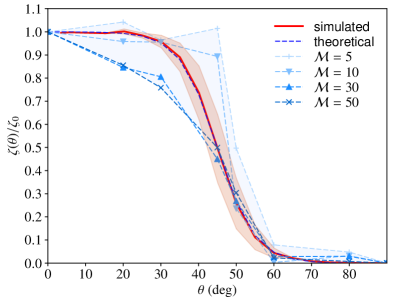
Figure 1: Functional dependence of the CR acceleration efficiency on the magnetic obliquity angle from hybrid PIC simulations of non-relativistic shocks (Caprioli & Spitkovsky, 2014). The blue points and dashed curves represent the results for different Mach numbers ranging from $\mathcal{M}=5$ to $50$, normalized to the maximum efficiency, respectively. The red curve represents our analytical model (equation 7). All hybrid PIC simulations exhibit a sharp drop of the acceleration efficiency at the critical angle for shock acceleration, $\theta_{\mathrm{crit}}=45^{\circ}$. The coloured red region around our analytical model shows the accuracy of recovering this functional form in our 3D shock tube simulations (see Fig. 2).

2 Methodology

Here we present our methodology and explain the numerical algorithms to implement magnetic obliquity dependent CR acceleration. We then validate our implementation with shock tube simulations that exhibit homogeneous magnetic fields. Finally, we lay down our procedure of setting up a turbulent magnetic field that finds application in Sedov-Taylor explosions in Sect. 3.

$\theta$	$\sqrt{\textbf{{B}}^{2}}$	$\rho_{\mathrm{l}}$	$\rho_{\mathrm{r}}$	$P_{\mathrm{l}}$	$P_{\mathrm{r}}$	$X^{\mathrm{cr}}_{\mathrm{l}}$	$X^{\mathrm{cr}}_{\mathrm{r}}$	$r_{\mathrm{c}}$	$\mathcal{M}_{1}$	$\gamma_{\mathrm{eff}}$
0∘	10-6	1	0.125	51.516	0.1	2	1	4.78	9.56	1.50
45∘	10-6	1	0.125	51.516	0.1	2	1	4.28	9.78	1.58
90∘	10-6	1	0.125	51.516	0.1	2	1	3.90	10.00	1.66

Table 1: Initial setup for the shock tubes shown in Fig. 2. The columns show magnetic obliquity $\theta$, magnetic field strength $\sqrt{\textbf{{B}}^{2}}$, initial mass density on the left- and right-hand sides, $\rho_{\mathrm{l}}$ and $\rho_{\mathrm{r}}$, total pressure on the left- and right-hand sides, $P_{\mathrm{l}}$ and $P_{\mathrm{r}}$, CR-to-thermal pressure ratio on the left- and right-hand sides, $X^{\mathrm{cr}}_{\mathrm{l}}$ and $X^{\mathrm{cr}}_{\mathrm{r}}$. The resulting shock has a compression ratio, $r_{\mathrm{c}}$, Mach number $\mathcal{M}_{1}$, and effective adiabatic index in the post-shock regime $\gamma_{\mathrm{eff}}$ (see equation 12).

2.1 Simulation method

All simulations in this paper are carried out with the massively parallel code arepo (Springel, 2010) in which the gas physics is calculated on a moving Voronoi mesh, using an improved second-order hydrodynamic scheme with the least-squares-fit gradient estimates and a Runge-Kutta time integration (Pakmor et al., 2016). We calculate the fluxes across the moving interface from the reconstructed primitive variables using the HLLD Riemann solver (Miyoshi & Kusano, 2005). We follow the equations of ideal MHD coupled to a second, CR fluid using cell-centred magnetic fields and the Powell et al. (1999) scheme for divergence control (Pakmor et al., 2011; Pakmor & Springel, 2013).

We model the relativistic CR fluid with an adiabatic index $\gamma=4/3$ and account for diffusive shock acceleration of CRs at resolved shocks in the computational domain, following a novel scheme (Pfrommer et al., 2017a). In our subgrid model for CR acceleration, we assume that diffusive shock acceleration operates efficiently provided there are favorable conditions (e.g., Sect. 2.2). This can be realized in the physical scenario, in which the current associated with the forward streaming CRs excites the non-resonant hybrid instability (Bell, 2004). This leads to exponential growth of magnetic fluctuations until the instability saturates at equipartition with the kinetic energy flux. This also implies efficient pitch angle scattering of CRs so that they approach the Bohm limit of diffusion. In such a situation, we can calculate the CR precursor length for the pressure-carrying protons between 1 to 10 GeV,

$$L_{\mathrm{prec}} \sim\sqrt{\kappa_{\mathrm{Bohm}}t}$$ (1)

$$\sim 0.001\,\mathrm{pc}\left(\frac{pc}{10\,\mathrm{GeV}}\right)^{1/2}\left(\frac{B}{100\,\mu\mathrm{G}}\right)^{-1/2}\left(\frac{t}{10^{3}\,\mathrm{yr}}\right)^{1/2}.$$

The CR precursor length only raises to 0.1 pc for TeV CRs gyrating in $\mu$G fields, which is still smaller than the numerical resolution $\Delta x=0.125$ pc of our simulations and thus unresolved (assuming a typical box size of 25 pc and $200^{3}$ grid cells for SNR simulations). Hence, in the interest of a transparent setup, we only model the dominant advective CR transport and neglect CR diffusion and streaming.

Similarly, we only account for adiabatic CR losses and neglect non-adiabatic CR losses such as Coulomb, hadronic and Alfvén-wave losses. In particular, we neglect the small effect of energy loss from the blast wave due to CRs escaping upstream. This effect softens the Sedov-Taylor solution from $r_{s}\propto t^{0.4}$ to $r_{s}\propto t^{0.39}$ (Bell, 2015). That calculation assumed a momentum spectrum of $p^{-4}$, which provides an upper limit to the energy contribution of escaping high-energy CRs. For observationally inspired softer spectra, the softening of the Sedov-Taylor solution becomes even smaller, thus justifying our neglect.

To localize shocks and their up- and downstream properties during the run time of the simulation, we adopt the method by Schaal & Springel (2015) that is solely based on local cell-based criteria. The method identifies the direction of shock propagation in Voronoi cells that exhibit a converging flow with the negative gradient of the pseudo-temperature that is defined as

$$kT^{*}=\frac{P}{n}=\frac{\mu m_{\mathrm{p}}(P_{\mathrm{th}}+P_{\mathrm{cr}})}{\rho},$$ (2)

where $n$ is the number density, $m_{\mathrm{p}}$ is the proton rest mass, and $\mu$ is the mean molecular weight. Hence, the shock normal is given by

$$\bm{\hat{n}}_{\mathrm{s}}=-\frac{\bm{\nabla}T^{*}}{\left|\bm{\nabla}T^{*}\right|}.$$ (3)

Voronoi cells with shocks are identified with (i) a maximally converging flow along the direction of shock propagation, while (ii) spurious shocks such as tangential discontinuities and contacts are filtered out, and (iii) the method provides a safeguard against labelling numerical noise as physical shocks. In particular, in our study the magnetic field is dynamically irrelevant at the shock, such that the non-MHD jump conditions are valid. Typically, shocks in arepo are numerically broadened to a width of two to three cells. By extending the stencil of the shock cell into the true pre- and post-shock regime, we determine the Mach number and dissipated energy of the shock. This enables us to inject a pre-determined energy fraction into our CR fluid into those Voronoi cells that exhibit a shock and into the adjacent post-shock cells (see Pfrommer et al., 2017a, for more details).

2.2 Obliquity-dependent CR acceleration

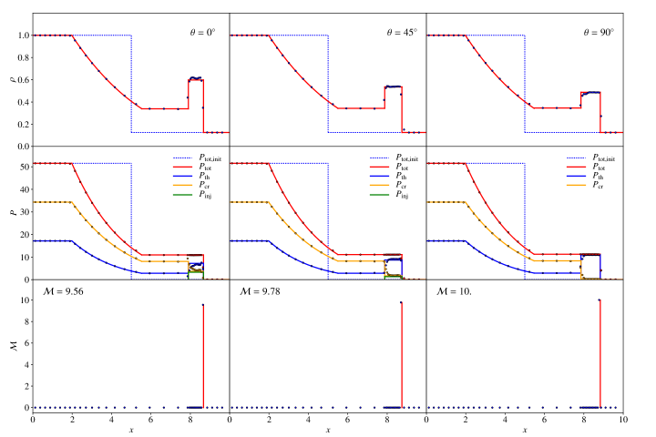
Figure 2: Shock-tube tests for different magnetic field orientations that account for pre-existing and freshly accelerated CRs (solid lines show the analytic solution of Pfrommer et al. (2017a), data points show mean simulation values, each averaged over 250 Voronoi cells). Shown are 3D simulations at time $t=0.35$. For each simulation we show density $\rho$, pressure $P$ and Mach number (top to bottom). The left panels show the simulation with a parallel magnetic shock configuration ($\theta=0$), where the acceleration efficiency $\zeta$ is maximized. The middle panels adopt an oblique configuration with $\theta=45^{\circ}$. We notice that the post-shock gas is less dense in comparison to the parallel case due to the smaller CR pressure as a result of a lower acceleration efficiency. In the right column, we show a perpendicular magnetic configuration ($\theta=90^{\circ}$), for which CR acceleration is completely inefficient. In this case, the shock propagates fastest (i.e., with the largest Mach number $\mathcal{M}$) of all three cases for otherwise identical initial conditions because of the absence of freshly injected CRs in the post-shock gas, which results in the hardest adiabatic index of $\gamma=5/3$ in the post-shock regime.

We adopt the following relation between the injected CR energy, $\Delta E_{\mathrm{cr}}$ and the dissipated energy at the shock, $E_{\mathrm{diss}}$,

$$\Delta E_{\mathrm{cr}}=\zeta(\mathcal{M}_{1},\theta)E_{\mathrm{diss}}.$$ (4)

The injection efficiency $\zeta(\mathcal{M}_{1},\theta)$ depends on the shock Mach number, $\mathcal{M}_{1}=v_{\mathrm{s}}/c_{1}$ (i.e., the shock speed in units of the pre-shock sound speed, $c_{1}$) and the upstream magnetic obliquity, $\theta$, defined as the angle between the normal to the shock front, $\textbf{{n}}_{\mathrm{s}}$, and the direction of the magnetic field, $\bm{\hat{b}}=\textbf{{B}}/|\textbf{{B}}|$:

$$\cos\theta=\bm{\hat{n}}_{\mathrm{s}}\mathchoice{\mskip 3.0mu\lower 0.86108pt\hbox{\scalebox{1.5}{$\cdot$}}\mskip 3.0mu}{\mskip 3.0mu\lower 0.86108pt\hbox{\scalebox{1.5}{$\cdot$}}\mskip 3.0mu}{\lower 1.29167pt\hbox{\scalebox{1.2}{$\cdot$}}}{\lower 1.29167pt\hbox{\scalebox{1.2}{$\cdot$}}}\bm{\hat{b}}.$$ (5)

Since the physics does not depend on the actual direction of the unit vectors $\bm{\hat{n}}_{\mathrm{s}}$ and $\bm{\hat{b}}$ (i.e., whether the vectors point in the same quadrant or not), we re-define the magnetic obliquity via

$$\theta=\arccos(|\cos\theta|)$$ (6)

In practice, for every shocked cell we collect the magnetic obliquity in the corresponding pre-shock region and communicate it to the shocked cell.

We calibrate $\zeta(\mathcal{M}_{1},\theta)$ with hybrid PIC simulations performed by Caprioli & Spitkovsky (2014). The authors find that DSA of ions is very efficient at quasi-parallel shocks, producing non-thermal ion spectra with the expected universal power-law distribution in momenta equal to $p^{-4}$. At very oblique shocks, ions can be accelerated via shock drift acceleration, but they only gain a factor of a few in momentum, and their maximum energy does not increase with time. In this paper, we only consider strong shocks (i.e., $\mathcal{M}_{1}\gg 1$) for which the injection efficiency saturates to a maximum value, $\zeta_{0}$. The saturation happens for shocks with $\mathcal{M}\gtrsim 30$, according to Kang & Ryu (2013).

Hence, we only need to model the scaling of the injection efficiency with magnetic obliquity, which is shown in Fig. 1 for different shock strengths. All simulated curves of the injection efficiency (light blue curves in Fig. 1) show a similar qualitative behavior: saturation at quasi-parallel shocks, a steep decline at the threshold obliquity of $\theta_{\mathrm{crit}}\simeq 45^{\circ}$, and leveling off at zero for quasi-perpendicular shocks. However, at a given magnetic obliquity, the function $\zeta(\theta,\mathcal{M})$ is not always monotonically rising with Mach number and shows substantial scatter (see Fig. 3 of Caprioli & Spitkovsky, 2014). Hence, we decided to capture the qualitative behavior of all four curves of the normalized injection efficiency, $\zeta(\theta,\mathcal{M})/\zeta_{0}$, for different shock strengths with the following functional form:

$$\zeta(\theta)\simeq\dfrac{\zeta_{0}}{2}\left[\tanh\left(\dfrac{\theta_{\mathrm{crit}}-\theta}{\delta}\right)+1\right].$$ (7)

We adopted a threshold obliquity of $\theta_{\mathrm{crit}}=\pi/4$ and a shape parameter of $\delta=\pi/18$ (red curve in Fig. 1). Hybrid PIC simulations by Caprioli & Spitkovsky (2014) demonstrate that the CR ion acceleration efficiency saturates for large Mach numbers at a value of $\zeta_{0}\simeq 0.15$. In our simulations however, we adopt a maximum acceleration efficiency of $\zeta_{0}=0.5$ to amplify the (dynamical) effects of CR acceleration. We checked that reducing the acceleration efficiency to realistic values results in qualitatively similar effects, albeit with a smaller amplitude.

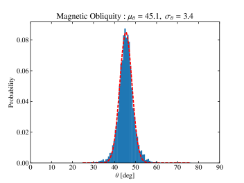
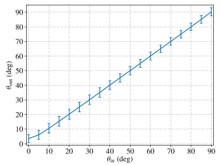
Figure 3: Left: probability distribution function (PDF) of the magnetic obliquity for a shock-tube simulation with initial obliquity of $45^{\circ}$. To increase the statistics, we use obliquity values of all shocked cells for 40 equally-spaced snapshots of that simulation and fit the mean and variance of a Gaussian distribution (red dashed) to the PDF (blue histogram). Right: comparison between the intrinsic ($\theta_{\mathrm{in}}$) and recovered magnetic obliquity ($\theta_{\mathrm{out}}$) for different shock-tube simulations. We recover the initial obliquity with an accuracy of $\sigma_{\theta}=3.4^{\circ}$ for all simulations except for the case $\theta=0$ (which is however of little practical relevance due to the very similar shock acceleration efficiencies in this regime).

2.3 Code validation with shock tubes

To validate our implementation and to test the correctness of our obliquity dependent shock acceleration algorithm, we performed several Riemann shock-tube simulations with different orientations of the magnetic field. A solution to the shock-tube problem with accelerated CRs is derived analytically in Pfrommer et al. (2017a) for a purely thermal gas and for a composite of thermal gas and pre-existing CRs. In the limit of weak background magnetic fields the solutions proposed in Pfrommer et al. (2017a) are still applicable. We simulate three-dimensional (3D) shock tubes with initially $10^{4}$ cells in a box of dimension $10\times 1\times 1$. The initial Voronoi mesh is generated by randomly distributing mesh-generating points in the simulation box and relaxing the mesh via Lloyd’s algorithm (1982) to obtain a glass-like configuration. All other initial parameters are laid down in Table 1.

In Fig. 2, we show three simulations with characteristically different magnetic obliquities, $\theta=0^{\circ},45^{\circ}$, and $90^{\circ}$. Our choice of a larger total pressure on the left-hand side (with the tube initially at rest), implies a rightwards moving shock, which is followed by a contact discontinuity, as well as a leftwards moving rarefaction wave. We show mean simulation values of density, pressure and Mach number, each averaged over 250 Voronoi cells to ensure an identical Poisson error per bin and to demonstrate the change of volume at the shock and over the rarefaction wave as a result of the moving-mesh nature of arepo.

Changing the orientation of the magnetic field from quasi-parallel ($\theta\gtrsim 0^{\circ}$) to quasi-perpendicular geometries ($\theta\lesssim 90^{\circ}$), the acceleration process becomes less and less efficient (as manifested from the fractions of post-shock CR pressure, see second row in Fig. 2). In the case of $\theta=90^{\circ}$, CR acceleration is absent and the purely thermal case is restored with a compression ratio of $r=3.9$ (for the adopted initial conditions). In the first column of Fig. 2 ($\theta=0^{\circ}$), we see an increased compressibility of the post-shock gas over the thermal case due to the abundantly produced CRs, which yields a shock compression ratio of $r=4.78$. Because of mass conservation, the shock cannot advance as fast in comparison to the purely thermal case and the Mach number is accordingly lower.

Our implementation records the magnetic obliquity in the upstream of the shocked Voronoi cells. In the left panel of Figure 3, we present the probability distribution function for $\theta$ for the intermediate case $\theta=45^{\circ}$. To improve our statistics, we used 40 different snapshots. We find normally distributed obliquity values around the expected value, with a standard deviation of $3.4^{\circ}$. We repeated the experiment for 18 simulations with an input obliquity that differed by $5^{\circ}$ from the preceding simulation. The correspondence between injected angles $\theta_{\mathrm{in}}$ and simulated angles $\theta_{\mathrm{out}}$ of shocked Voronoi cells becomes apparent in the right panel of Figure 3, with a 1-sigma accuracy of $3.4^{\circ}$. This accuracy is numerically converged as we show in Appendix A. We only observe a small numerical deviation at small obliquities $\theta_{\mathrm{in}}<3^{\circ}$. However, the resulting acceleration efficiency is not affected due to the constant efficiency at quasi-parallel shocks.

2.4 Turbulent magnetic fields

In order to generate turbulent magnetic fields with an average value $\langle\textbf{{B}}\rangle=\mathbf{0}$ but $\langle\sqrt{\textbf{{B}}^{2}}\rangle\neq 0$, we adopt a magnetic power spectrum of Kolmogorov type and scale the field strength to an average plasma beta factor of unity. The three components of the magnetic field $B_{i}$ ($i\in\{1,2,3\}$) are treated independently to ensure that the final distribution of $\textbf{{B}}(\textbf{{x}})$ has a random phase. To proceed, we assume Gaussian-distributed field components that follow a one-dimensional power spectrum $P_{i}(k)$, defined as $P_{i}(k)\propto k^{2}|\tilde{B}_{i}(k)|^{2}$, of the form

$$|\tilde{B}_{i}(k)|^{2}=\begin{cases}A,&k<k_{\mathrm{inj}},\\ A\left(\dfrac{k}{k_{\mathrm{inj}}}\right)^{-11/3},&k_{\mathrm{inj}}\leq k,\end{cases}$$ (8)

where $A$ is normalization constant, $k=|\textbf{{k}}|$, and $k_{\mathrm{inj}}$ is the injection scale of the field. Modes on larger scales ($k<k_{\mathrm{inj}}$) follow a white noise distribution and modes with $k>k_{\mathrm{inj}}$ obey a Kolmogorov power spectrum. For each magnetic field component, we set up a complex field such that

$$[\Re(\tilde{B}_{i}(\bm{k})),\Im(\tilde{B}_{i}(\bm{k}))]=[G_{1}(X_{1},X_{2})\sigma_{k},G_{2}(X_{1},X_{2})\sigma_{k}],$$ (9)

where $G_{i}$ ($i\in\{1,2\}$) is a distribution of uniform random deviates $X_{1}$ and $X_{2}$ that returns Gaussian-distributed values. We set the corresponding standard deviation $\sigma_{k}$ to $\tilde{B}_{i}$ for every value of $k$. We normalize the spectrum to the desired variance of the magnetic field components in real space, $\sigma_{B}$ using Parseval’s theorem,

$$\sigma_{B}^{2}=\dfrac{1}{N^{2}}\sum_{k}^{N}|\tilde{B}_{i}(k)|^{2}.$$ (10)

We then subtract the radial field component in $k$ space to fulfill the constraint $\mathrm{div}\textbf{{B}}=0$, via

$$\tilde{\textbf{{B}}}_{k}\to\tilde{\textbf{{B}}}_{k}-\bm{\hat{k}}(\bm{\hat{k}}\mathchoice{\mskip 3.0mu\lower 0.86108pt\hbox{\scalebox{1.5}{$\cdot$}}\mskip 3.0mu}{\mskip 3.0mu\lower 0.86108pt\hbox{\scalebox{1.5}{$\cdot$}}\mskip 3.0mu}{\lower 1.29167pt\hbox{\scalebox{1.2}{$\cdot$}}}{\lower 1.29167pt\hbox{\scalebox{1.2}{$\cdot$}}}\tilde{\textbf{{B}}}_{k}).$$ (11)

Applying an inverse fast Fourier transform to $\tilde{\textbf{{B}}}_{k}$ and re-scaling the magnetic field to the desired average magnetic-to-thermal pressure ratio yields a turbulent magnetic field distribution. To ensure pressure equilibrium in the initial conditions, we adopt temperature fluctuations of the form $nk_{\mathrm{B}}\delta T=-\delta\textbf{{B}}^{2}/(8\pi)$. This setup does not balance the magnetic tension force. The resulting turbulent motions have a small amplitude in comparison to the velocity of the expanding blast wave so that to good approximation, the ambient gas can be considered frozen and does not contribute to the dynamics.

3 Sedov-Taylor explosions

In order to understand the non-thermal properties of supernova remnants, we model the explosion as an expanding Sedov-Taylor blast wave in the magnetised interstellar medium. After deriving an analytical solution for the Sedov-Taylor problem in the presence of CR acceleration with an arbitrary shock acceleration efficiency, we study magnetic obliquity dependent CR acceleration in homogeneous and turbulent fields with varying coherence scales and formulate an analytic theory that enables us to obtain the average CR efficiency.

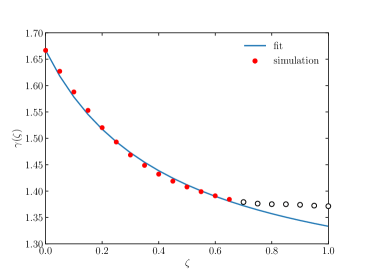
Figure 4: Effective ratio of specific heats $\gamma$ as a function of CR acceleration efficiency $\zeta$ for the Sedov-Taylor blast wave (ignoring the obliquity dependence of CR acceleration). The simulations (dots) and analytical fit (solid, equation 15) interconnect the thermal gas case without CR acceleration (${\zeta=0}$) and the opposite extreme of a (hypothetical) 100% efficient acceleration process, which yields a fully relativistic gas in the post-shock region ($\gamma=4/3$). The simulations do not reproduce the limit $\gamma\to 4/3$ for $\zeta\to 1$ due to residual thermalization.

3.1 Analytical solution with CR acceleration

Parameter	Value	Approximation
$a$	1.185	32/27
$b=20/3-9a+3a^{2}$	0.214	52/243
$c=4-3a$	0.445	4/9

Table 2: Best-fit parameters of the effective ratio of specific heats as a function of CR acceleration efficiency, $\gamma(\zeta)$, of equation (15) for the Sedov-Taylor blast-wave problem. The fit and the simulated points are shown in Fig. 4

First, we derive analytical exact solutions of the Sedov-Taylor blast-wave problem with CR acceleration without an obliquity dependent efficiency. If a substantial fraction of the dissipated energy is converted into CRs, this alters the effective adiabatic index $\gamma_{\mathrm{eff}}$ that is defined as the logarithmic derivative of the total pressure with respect to density at constant entropy $s$:

$$\gamma_{\mathrm{eff}}\equiv\left.\frac{\mathrm{d}\ln(P_{\mathrm{cr}}+P_{\mathrm{th}})}{\mathrm{d}\ln\rho}\right|_{s}=\frac{\gamma_{\mathrm{cr}}P_{\mathrm{cr}}+\gamma_{\mathrm{th}}P_{\mathrm{th}}}{P_{\mathrm{cr}}+P_{\mathrm{th}}},$$ (12)

Subsequently the radius of the explosion is modified as it depends on the compressibility of the post-shock gas in the interior of the blast wave.

In the case of a single polytropic fluid, the shock radius of the blast wave evolves self similarly according to

$$r_{\mathrm{s}}(t)=\left(\frac{E_{1}}{\alpha\rho_{1}}\right)^{1/5}t^{2/5},$$ (13)

where $t$ is the time since explosion and $\alpha$ is a self-similarity parameter that depends on the effective adiabatic index, which itself is a function of CR shock acceleration efficiency $\zeta$. To determine this relation, we run a set of simulations, varying $\zeta\in[0,1]$ in steps of 0.05. In each simulation, we determine the average shock radii at different times and obtain $\alpha(\zeta)$ via equation (13).

In Appendix B, we numerically solve the self-similar, spherically symmetric conservation equations of mass, momentum and energy to determine the behavior of $\alpha(\gamma)$. We find an analytical fit to the solution of the form

$$\alpha(\gamma)\approx\dfrac{16}{75}\left[\dfrac{\pi(3\gamma-1)}{(\gamma-1)(\gamma+1)^{2}}-\dfrac{3}{8}\right],$$ (14)

which has an accuracy of approximately 0.8%. Combining $\alpha(\zeta)$ (obtained with our simulations with CR acceleration and via equation 13) and $\alpha(\gamma)$ (equation 14), we arrive at an expression of the effective adiabatic index as a function shock acceleration efficiency, $\gamma(\zeta)$, as shown in Fig. 4. In particular, an efficiency of $\zeta=0.5$ corresponds to an effective ratio of specific heats of $\gamma\simeq 1.408$. As seen in Fig. 4, the simulations do not reproduce the limit $\gamma\to 4/3$ for $\zeta\to 1$ due to residual thermalization. Note that this case is purely academic and likely not realised in Nature. Hence, we fit our simulation values for $\zeta\leq 0.65$ with an equation of the form

$$\gamma(\zeta)=a+\dfrac{b}{c+\zeta},$$ (15)

subject to the boundary condition of $\gamma=5/3$ for $\zeta=0$ and 4/3 for $\zeta=1$. This allows to express the parameters $b$ and $c$ solely as a function of $a$. The corresponding parameters satisfying these requirements are shown in Table 2. Adopting the rational approximation of these fitting parameters (Table 2) we obtain

$$\gamma(\zeta)=\dfrac{4}{3}\left(\dfrac{8\zeta+5}{9\zeta+4}\right).$$ (16)

Combining this result with equation (14), we get a comprehensive formula for the self-similarity parameter in equation (13) as a function of the acceleration efficiency $\zeta$:

$$\alpha({\zeta})=\dfrac{2}{25}\left[\dfrac{72\pi(9\zeta+4)^{2}(23\zeta+16)}{(5\zeta+8)(59\zeta+32)^{2}}-1\right].$$ (17)

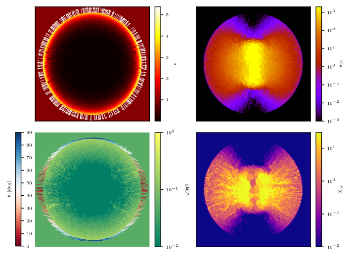
Figure 5: Sedov-Taylor blast wave with obliquity dependent CR acceleration expanding into a homogeneous magnetic field at $t=0.1$. Initially, the field is aligned with the horizontal direction. We show a 2D cross section of the density $\rho$ (top left) overplotted with normal vectors of the shock (as determined by our shock-finding algorithm); the specific CR energy $u_{\mathrm{cr}}$ (top right); the magnetic field strength $\sqrt{\textbf{{B}}^{2}}$ (bottom left) overplotted with the outwards directed orientations of the magnetic field at the shocked cells (colour coded by magnetic obliquity $\theta$) and the CR-to-thermal pressure ratio $X_{\mathrm{cr}}$ (bottom right). We can see that the specific CR energy exhibits a quadrupolar anisotropy, with the maximum in the direction of the magnetic field (quasi-parallel shock configuration). The increased density in this quasi-parallel direction (due to the higher compressibility of the CR-enriched post-shock plasma) implies a slower shock expansion velocity and hence a slightly oblate shock surface with the two long axis aligned perpendicular to the ambient field direction. Note that the shock compression only amplifies the perpendicular magnetic field component, which re-aligns field vectors for oblique shocks.

3.2 CR acceleration in a homogeneous field

Our initial Voronoi mesh is generated by randomly distributing mesh-generating points in the unit box and relaxing the mesh via Lloyd’s algorithm (1982). The self-similarity of the problem, which is not broken by CR acceleration (Pfrommer et al., 2017a), allows us to use scale free units. We use a box of $200^{3}$ cells to ensure convergence also at early times. Throughout the simulation box, we adopt a uniform density of $\rho_{1}=1$, a negligible pressure of $P_{1}=10^{-4}$, a zero initial velocity, and a thermal adiabatic index of $\gamma=5/3$. At time $t=0$, we inject thermal energy of $E_{1}=1$ into the central mesh cell. We follow ideal MHD without self-gravity and adopt a maximum acceleration efficiency of $\zeta_{0}=0.5$ to amplify the (dynamical) effects of CR acceleration.

First, we adopt a homogeneous magnetic field in the box that is oriented along the $x$ axis and a plasma beta of $\beta=1$. In Fig. 5 we show maps of different quantities in the equatorial plane at $t=0.1$, namely the mass density $\rho$ (with the shock normal as measured in situ in the simulations and shown in white), the specific CR energy $u_{\mathrm{cr}}$, the magnetic field strength $\sqrt{\textbf{{B}}^{2}}$ (with the magnetic orientations at the shock colour coded by upstream magnetic obliquity), and the CR-to-thermal pressure ratio $X_{\mathrm{cr}}=P_{\mathrm{cr}}/P_{\mathrm{th}}$.

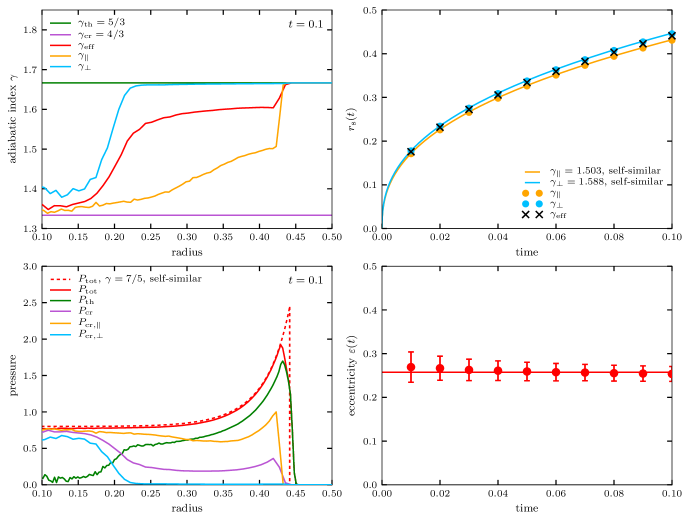
Figure 6: Radial profiles of characteristic quantities of the Sedov-Taylor explosion with obliquity dependent CR acceleration. The top left panel shows the radial profile of the effective adiabatic index. The adiabatic index in the direction perpendicular to the magnetic field (light blue) raises quickly to values comparable with the thermal adiabatic index $5/3$ (green) whereas the adiabatic index in the direction parallel to B (yellow) deviates only at larger radii from the relativistic value of $4/3$ (violet). The red line represents the effective adiabatic index averaged over all directions. The bottom left panel shows the corresponding radial profiles of the CR pressure in the different directions. The thermal pressure dominates at larger radii while the CR pressure drops significantly outside the center. The top right panel represents the time evolution of the shock radius in the direction of the magnetic field (yellow) and perpendicular to it (light blue). Effective CR acceleration for quasi-parallel shock configurations yields an increased compressibility and hence a slower propagating shock. This is quantified in the time evolution of the shock eccentricity in the bottom right panel. The constant eccentricity of the oblate shock (within the uncertainties) demonstrates self-similar evolution of the blast wave also in this case.

The unit vectors of the shock normal in the top left panel of Fig. 5 show a deviation from spherical symmetry with a smaller shock radius and an enhanced density in the direction parallel and anti-parallel to the magnetic field. This is the immediate consequence of obliquity-dependent shock acceleration with copious CR production at quasi-parallel shocks, which is accompanied by an increased compressibility due to the softer equation of state of the composite fluid of CRs and thermal gas. This is manifested in the quadrupolar morphology of $u_{\mathrm{cr}}$ with the axis of symmetry aligned with the magnetic field orientation (top right of Fig. 5). The morphology of $u_{\mathrm{cr}}$ is echoed by $X_{\mathrm{cr}}$ (bottom right of Fig. 5). Adiabatic expansion of a composite of CRs and thermal gas eventually yields a dominating CR pressure in the interior of the explosion for quasi-parallel shock geometries, at $|\theta|\lesssim\pi/4$.

An oblique shock only amplifies the perpendicular field component and leaves the parallel component invariant. This re-orients the oblique magnetic field towards the shock surface and increases the field strength at quasi-perpendicular shocks (bottom left of Fig. 5). Our strongly magnetised background plasma with $\beta=1$ becomes very weakly magnetised at the shock since the adiabatic increase of magnetic pressure falls orders of magnitudes short in comparison to the shock-dissipated thermal pressure at our strong Sedov-Taylor shock. Hence, the magnetic field merely impacts the dynamics of the blast wave through the magnetic obliquity-dependent shock acceleration of CRs and not through its pressure.

This analysis is quantified in Fig. 6, where we show radial profiles of different volume-weighted quantities, such as the effective ratio of heat capacities $\gamma_{\mathrm{eff}}$, the pressure, and the time evolution of the shock radius and eccentricity of the oblate blast wave. The effective ratio of heat capacities $\gamma_{\mathrm{eff}}$ is computed from volume-averaged partial pressures of the CR and thermal gas components via equation 12. The top and bottom left panels of Fig. 6 show the radial variation of the effective adiabatic index $\gamma_{\parallel,\perp}$ and the partial pressures $P_{\parallel,\perp}$ for two regions: parallel and perpendicular. $\gamma_{\parallel}$ and $P_{\mathrm{cr},\parallel}$ are computed from cells that belong to the hourglass-shaped region inside the blast wave that was overrun by a quasi-parallel shock. Here, we define this quasi-parallel shocked region as a narrow double cone oriented along the original magnetic field with an opening angle of 20^∘. Similarly, we define the region overrun by quasi-perpendicular shocks as the complement of a wide double cone that is bounded by an equatorial band with latitude 20^∘.

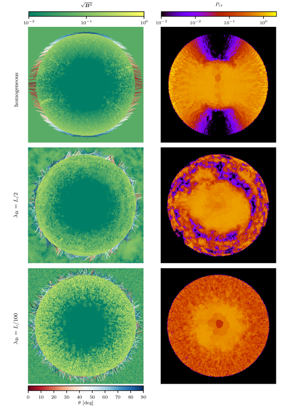
Figure 7: Cross-sections through the centre of 3D simulations of Sedov-Taylor explosions with obliquity-dependent CR acceleration. We show a simulation with a homogeneous, horizontally oriented magnetic field (first row), a turbulent magnetic field with a large correlation length of $\lambda_{B}=L/2$ (second row) and with a very small correlation length, $\lambda_{B}=L/100$, in comparison to the radius of the blast wave (third row). We depict magnetic field strength (left column) and CR pressure (right column). In the homogeneous field case we notice a quadrupolar CR distribution that is maximized for quasi-parallel shocks (visualised with red arrows in the left-hand panels) while the magnetic field is only adiabatically amplified at quasi-perpendicular shocks (blue arrows). In the second row we observe a patchy CR distribution with maxima at regions that were over-run with quasi-parallel shocks. The CR distribution in the case of small-scale turbulence (last row) is completely isotropic and the compression of the magnetic field is uniformly distributed across the shock.

The copious CR production at a quasi-parallel shock with the subsequent adiabatic expansion softens the adiabatic index to values close to that of a fully relativistic gas of 4/3. Since the region overrun by a quasi-perpendicular shock is characterized by a ratio of heat capacities close to a purely thermal gas, the effective adiabatic index $\gamma_{\mathrm{eff}}$ (shown in red) as well as the spherically averaged CR pressure (shown in purple) levels off at values in between.

The top-right panel of Fig. 6 shows the time evolution of the simulated shock radius (filled circles) and the self-similar analytic solution (continuous lines). In line with the previous discussion, the shock radius in the direction perpendicular to the ambient magnetic field moves faster than the shock in the (anti-)parallel direction owing to the increased compressibility of the latter due to efficient CR acceleration. The continuous lines are obtained by fitting the shock radius evolution (equation 13) in double-logarithmic space for $\alpha(\gamma)$. Inverting equation 14 yields the corresponding effective adiabatic factor shown in the figure. In between those two curves, we show the solution for the effective adiabatic index (crosses).

The increased compressibility of CR-enriched quasi-parallel shocks implies an oblate shock surface that is characterised by an eccentricity, defined as

$$\varepsilon(t)=\sqrt{1-\left[\dfrac{r_{\|}(t)}{r_{\bot}(t)}\right]^{2}}.$$ (18)

Due to the volumetric distribution of CRs with respect to the thermal gas, the influence of CR production affects the entire explosion. This renders it impossible to separate the cases of purely thermal and maximally efficient CR acceleration for the perpendicular and parallel shock radii, respectively. This means that a direct measurement of the eccentricity assuming a pure thermal $\zeta=0$ in the perpendicular direction and a CR-modulated $\zeta=\zeta_{0}$ in the parallel direction yields an incorrect result. Instead, an average efficiency $\langle\zeta\rangle$ is required to determine the average radius of the explosion, representing an intermediate case between the parallel and perpendicular shock radius. In the lower right panel of Fig. 6, we show the eccentricity of the oblate shock surface along with the uncertainty intervals assuming Gaussian statistics,

$$\Delta\varepsilon=\left(\dfrac{1-\varepsilon^{2}}{\varepsilon}\right)\sqrt{\left(\dfrac{\sigma_{\parallel}}{r_{\parallel}}\right)^{2}+\left(\dfrac{\sigma_{\perp}}{r_{\perp}}\right)^{2}}$$ (19)

where $\sigma_{\parallel}$ and $\sigma_{\perp}$ are the standard deviations of the shock radius in the direction of the magnetic field and perpendicular to it, respectively. We obtain the theoretical estimate for the eccentricity from our measured self-similar solutions for the parallel and perpendicular shock radii of the top-right panel in Fig. 6. There are two strategies to measure the eccentricity: first, determining the distance to the cells of the shock surface inside narrow cones or bands of equal latitude that are centered on the explosion and oriented along the magnetic field direction; second: measuring the momenta of inertia of the entire oblate shock surface, diagonalising the resulting tensor, determining the resulting eigenvalues and extracting the length of the three semi-axes. We decided in favor of the first method because it generates less numerical fluctuations.

We find a constant eccentricity of $\varepsilon=0.25\pm 0.02$ during the adiabatic expansion. Note that $\varepsilon$ depends on the average efficiency $\langle\zeta\rangle$ and is expected to be smaller for realistic maximum acceleration efficiencies of order 0.15. The constant eccentricity with time demonstrates that the Sedov-Taylor explosion remains self similar also in the presence of obliquity-dependent CR acceleration. In Appendix A we show that the measured eccentricity in our simulations is numerically converged for $100^{3}$ grid cells.

3.3 CR acceleration in a turbulent field

After studying magnetic obliquity-dependent CR acceleration at a Sedov-Taylor blast wave that propagates in a homogeneous magnetic field, we now turn to turbulent magnetic fields with different magnetic correlation lengths $\lambda_{B}=2\pi/k_{\mathrm{inj}}$. As initial conditions for the magnetic field, we adopt a Gaussian random field with a Kolmogorov power spectrum on scales smaller than the coherence length and a white-noise power spectrum on larger scales, as described in Sect. 2.4. The larger $\lambda_{B}$ in comparison to the shock radius, the fewer statistically independent regions of correlated magnetic fields there are inside the blast wave. Hence we introduce the magnetic coherence length in units of the shock radius, $\Lambda_{B}=\lambda_{B}/r_{\mathrm{s}}(t)$ as a new parameter. Blast waves with the same $\Lambda_{B}$ are statistically self similar.

We perform several simulations with different correlation lengths ranging from $\lambda_{B}=L$ to $\lambda_{B}=L/200$ for $200^{3}$-cell runs. In Fig. 7 we show different realizations of the CR pressure for varying the correlation lengths of the magnetic field and compare the results to our previous simulation with a homogeneous field. Correlated magnetic patches imply a similarly patchy CR distribution: regions that are overrun by quasi-parallel shocks are CR enriched whereas regions that have experienced quasi-perpendicular shocks result in voids without CRs. As the scaled correlation length $\Lambda_{B}$ becomes smaller, the magnetic obliquity also changes on smaller scales and the number of CR islands becomes more frequent to the point that they merge into a single (noisy) CR distribution. This case is similar to uniform CR acceleration (which is independent of magnetic obliquity), but exhibits a lower overall CR acceleration efficiency.

3.4 Average CR acceleration efficiency and field realignment

In order to understand the blast wave-averaged CR acceleration efficiency, we consider the two limiting cases of a homogeneous field and a fully turbulent field with a coherence scale of the initial grid resolution ($\lambda_{B}=\Delta L$) analytically. In the small-scale turbulent case, we consider a fixed shock normal pointing along $\bm{\hat{z}}$ without loss of generality. The magnetic field vector can then assume any direction on the upper half-sphere because CR acceleration does not depend on the sign of the magnetic field and is symmetric with respect to $\theta=0$. Hence, the probability distribution of the magnetic obliquity is given by $f(\theta)=\sin\theta$ with $\theta\in[0,\pi/2]$.

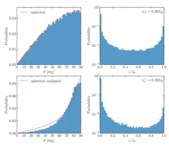
Figure 8: Probability distribution functions (PDFs) of the magnetic obliquity (left) and CR acceleration efficiency $\zeta$ (right) in the case of a homogeneous magnetic field in the upstream regime (top panels) and after accounting for magnetic re-orientation in the immediate downstream regime (bottom panels). Here, we adopt an artificially small value for the maximum CR acceleration efficiency of $\zeta_{0}=0.02$, which implies an almost spherical shock due to the negligible CR backreaction in this case. The obliquity distribution follows the theoretical expectation of $f(\theta)=\sin(\theta)$. Accounting for magnetic re-orientation at oblique shocks skews this distribution towards quasi-perpendicular geometries (bottom left), which can be analytically described by equation (31) for $\varepsilon=0$ (dashed line). Note that $\zeta$ follows a bimodal distribution as a result of the flatness of the efficiency function (equation 7) at quasi-perpendicular and -parallel shocks with a sharp transition in between.

Integrating the efficiency over this probability distribution results in the average efficiency according to

$$\langle\zeta\rangle=\int_{0}^{\pi/2}\zeta(\theta)\sin\theta\,\mathrm{d}\theta=\begin{cases}\zeta_{0}\left(1-\frac{\displaystyle 1}{\displaystyle\sqrt{2}}\right),&\mbox{for }\zeta=\zeta_{\mathrm{toy}},\\ 0.302\,\zeta_{0},&\mbox{with Equ.~{}(\ref{eq:efficiency}).}\end{cases}$$ (20)

Here, we introduced a toy example for the obliquity dependent acceleration that is represented by a discontinuous jump of the efficiency at $\theta_{\mathrm{crit}}$ from $\zeta_{0}$ to zero:

$$\zeta_{\mathrm{toy}}(\theta)=\zeta_{0}\Theta(\theta_{\mathrm{crit}}-\theta),$$ (21)

where $\Theta(x)$ is the Heaviside function, representing the limiting case of $\delta\rightarrow\infty$ in equation (7). This gives us a lower limit for the efficiency.

In the case of a homogeneous field, we fix the magnetic field vector in space and point it into the $z$ direction without loss of generality. Again, the shock normal can assume any direction on the upper half-sphere so that we obtain the same probability distribution function as in the small-scale turbulent case, $f(\theta)=\sin\theta$. The average CR shock acceleration efficiency is thus also given by equation (20).

We find that eccentricity plays an important role in shaping the probability distribution of the obliquity. To take this into account we define an ellipsoidal reference frame via

$$x=\left(h+\dfrac{a}{\sqrt{1-\varepsilon^{2}\cos^{2}\varphi}}\right)\sin\varphi\cos\lambda,$$ (22)

$$y=\left(h+\dfrac{a}{\sqrt{1-\varepsilon^{2}\cos^{2}\varphi}}\right)\sin\varphi\sin\lambda,$$ (23)

$$z=\left[h+\dfrac{(1-\varepsilon^{2})a}{\sqrt{1-\varepsilon^{2}\cos^{2}\varphi}}\right]\cos\varphi,$$ (24)

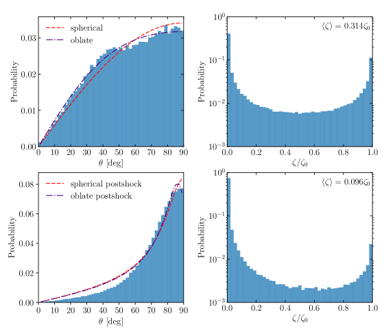
Figure 9: PDF of the magnetic obliquity (left) and CR acceleration efficiency $\zeta$ (right) in the case of a homogeneous magnetic field in the upstream regime (top panels) and after accounting for magnetic re-orientation (bottom panels) with a maximum efficiency of $\zeta_{0}=0.5$. The obliquity distribution in the top left panel follows our theoretical prediction $f(\theta,\varepsilon)$ (purple, equation 26) of an oblate expanding shock. For comparison, we also show the spherical PDF (red dashed, see Fig. 8). Accounting for magnetic re-orientation at oblique shocks skews this distribution towards quasi-perpendicular geometries (bottom left), which can be analytically described by equation (31).

where $\lambda$ and $\varphi$ are the longitude and pseudo-latitude from the ellipsoid, respectively, $h$ is the height above the surface of the ellipsoid, $a$ the semi-major axis, and $\varepsilon$ the eccentricity.

As shown in Appendix C, for a homogeneous magnetic field that points into the positive $z$ direction (short axis of the oblate ellipsoid) the angle $\varphi$ is by construction equal to the definition of the magnetic obliquity $\theta$. Using the fact that $\varphi\equiv\theta$, the Jacobian of this coordinate transformation on the oblate surface ($h=0$) is given by

$$S(\theta,\varepsilon)=\sin\theta\dfrac{1-\varepsilon^{2}}{(1-\varepsilon^{2}\cos^{2}\theta)^{2}}.$$ (25)

Hence, the normalized distribution function for the obliquity $\theta$ reads

$$f(\theta,\varepsilon)=S(\theta,\varepsilon)\left[\int_{0}^{\pi/2}S(\theta,\varepsilon)\mathrm{d}\theta\right]^{-1},$$ (26)

which reduces to $\sin\theta$ for $\varepsilon=0$.

For our simulations with $\zeta_{0}=0.5$, we obtain an eccentricity of $\tilde{\varepsilon}=0.25$, and hence an average efficiency of

$$\langle\zeta(\tilde{\varepsilon})\rangle=\int_{0}^{\pi/2}\zeta(\theta)f(\theta,\tilde{\varepsilon})\mathrm{d}\theta=0.316\zeta_{0}.$$ (27)

The error $\Delta\zeta$ on this quantity derives from the uncertainty on the eccentricity:

$$\Delta\tilde{\zeta}=\left.\dfrac{\partial\langle\zeta(\varepsilon)\rangle}{\partial\varepsilon}\right|_{\tilde{\varepsilon}}\Delta\tilde{\varepsilon}=\left.\left[\int_{0}^{\pi}\zeta(\theta)\dfrac{\partial f(\theta,\varepsilon)}{\partial\varepsilon}\right|_{\tilde{\varepsilon}}\mathrm{d}\theta\right]\Delta\tilde{\varepsilon}=0.002\zeta_{0},$$ (28)

such that the efficiency for this oblate reads

$$\tilde{\zeta}=(0.316\pm 0.002)\zeta_{0}.$$ (29)

Because we propagate the upstream value of the magnetic obliquity to the shock surface, the resulting obliquity distribution at the shock is expected to follow $f(\theta)=\sin(\theta)$ in the case of a sphere and equation (26) for ellipsoids.

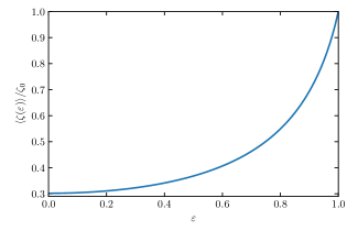
Figure 10: Average acceleration efficiency as a function of the eccentricity $\varepsilon$ of the oblate according to the distribution shown in equation (25) and equation (27) in a homogeneous magnetic field configuration. For $\varepsilon=0$ the original value of equation (20) is restored while for an eccentricity of unity the oblate degenerates into a circle, yielding everywhere a maximum efficiency.

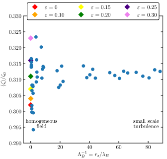
Figure 11: Average CR acceleration efficiency for a turbulent magnetic field with different correlation lengths $\Lambda_{B}=\lambda_{B}/r_{\mathrm{s}}(t)$. The case $\Lambda_{B}^{-1}=0$ corresponds to a homogeneous magnetic field and $\Lambda_{B}^{-1}=85$ relates to the small-scale turbulent case with a coherence scale equal to the initial grid resolution of our simulation. The coloured diamonds at $\Lambda_{B}^{-1}=0$ show the homogeneous field case for different average CR acceleration efficiencies corresponding to different eccentricities. The simulation points scatter around the value $\langle\zeta\rangle=(0.311\pm 0.005)\zeta_{0}$.

In the next step, we assess the distribution of downstream magnetic obliquity as a result of realignment of the tangential component of the magnetic field due to the shock. We can estimate the obliquity after magnetic realignment with the aid of the Rankine-Hugoniot jump conditions:

$$\cos\theta_{2}(r_{\mathrm{c}})=\dfrac{\cos\theta_{1}}{\sqrt{\cos^{2}\theta_{1}+r_{\mathrm{c}}^{-2}\sin^{2}\theta_{1}}}$$ (30)

where $r_{\mathrm{c}}$ is the compression ratio at the shock. We can then insert this formula into equation (25) to obtain the expected distribution of realigned angles for oblates:

$$f[\theta(r_{\mathrm{c}}),\varepsilon]=S[\theta(r_{\mathrm{c}}),\varepsilon]\left[\int_{0}^{\pi/2}S[\theta(r_{\mathrm{c}}),\varepsilon]\mathrm{d}\theta\right]^{-1}$$ (31)

which reduces to $\sin[\theta(r_{\mathrm{c}})]$ for $\varepsilon=0$. We find good agreement of these theoretical distributions and our simulations in Figs. 8 and 9 for a maximum efficiency of $\zeta_{0}=0.02$ and of $\zeta_{0}=0.5$, respectively. Note that the low CR acceleration efficiency in Fig. 8 allows to neglect the geometrical anisotropy of the shock surface that results from copious CR production in the direction of the magnetic field. In all cases, we find a bimodal distribution of $\zeta$ as a result of the flat efficiencies at quasi-perpendicular and -parallel shocks with a sharp transition in between. We also find a good agreement of the realigned obliquity distributions, which are skewed towards quasi-perpendicular geometries.

The effect of an oblate geometry becomes evident in Fig. 9 (upper left panel), which shows an improved fit of the elliptical distribution in comparison to the spherical sinusoidal distribution. However, the resulting shape of the efficiency distribution is only little affected. Thus, its average value is only slightly increased over the spherical case as can be inferred from Figs. 8 and 9. The full evolution of $\langle\zeta\rangle$ as a function of $\varepsilon$ is shown in Fig. 10. The academic case of $\varepsilon=1$ represents an unphysical limit where the oblate degenerates into a circle. This orients the shock surface in such a way so that it is always parallel to the direction of the magnetic field and yields the maximum possible acceleration efficiency.

In Fig. 11 we summarize results for different simulations with varying correlation lengths of $\lambda_{B}^{-1}=[2,4,10,20,50,100,150,200]$ each at times $t=[5,6,7,8,9,10]\times 0.01$ in simulation units. The expanding shock front starts to embrace more and more coherent magnetic patches whose number scales as $N\propto\Lambda_{B}^{-3}$. For comparison, we also show the theoretically expected eccentricities for the homogeneous field case with coloured diamonds. There is no trend in the evolution of the average acceleration efficiency as a function of $\Lambda_{B}^{-1}$. Instead, the simulation values scatter between an eccentricity of $\varepsilon=0.10$ (orange diamond) and $\varepsilon=0.3$ (violet diamond), yielding a value of $\langle\zeta\rangle=(0.311\pm 0.05)\zeta_{0}$. For $\lambda_{B}\gg\Delta L$, CR-rich patches give rise to corrugations of the shock surface causing local small deviations from spherical symmetry. If the correlation length becomes comparable to the initial grid resolution then the blast wave becomes spherical, albeit with a slightly higher efficiency.

4 Conclusions

In this paper we perform MHD simulations of the evolution of supernova remnants in the Sedov-Taylor phase. For the first time, we model magnetic obliquity dependent CR acceleration and study i) its dynamical effects on the overall evolution of the blast wave and ii) how different magnetic geometries affect the resulting CR distribution. To this end, we use results from hybrid PIC simulations (with kinetic ions and fluid electrons) of non-relativistic, large Mach number shocks. Those demonstrate that only quasi-parallel magnetic shock configurations can accelerate ions while quasi-perpendicular shocks are ineffective.

Using idealized shock tube experiments, we show that our algorithm is able to recover the input direction of the magnetic field with a Gaussian scatter of around $3^{\circ}$. When we change the magnetic orientation from quasi-perpendicular to quasi-parallel configurations, the efficiency of CR acceleration and the associated post-shock compressibility increase. This leads to density jumps that exceed the theoretical limit $\rho_{2}/\rho_{1}=4$ (valid for a thermal gas), slows down the shock and decreases the Mach number.

We derive analytical exact solutions of the Sedov-Taylor blast-wave problem with CR acceleration (neglecting obliquity dependent effects). We numerically solve the self-similar, spherically symmetric conservation equations of mass, momentum and energy to determine the behavior of the shock radius. This enables us to derive analytical fitting functions for the effective ratio of specific heats for a composite of thermal gas and CRs as a function of the maximum acceleration efficiency.

Our simulations of the Sedov-Taylor blast wave problem with obliquity dependent CR acceleration in a homogeneous magnetic field geometry show the emergence of an oblate ellipsoidal shock surface. Its short axis is aligned with the ambient magnetic field orientation due to the efficient CR acceleration at quasi-parallel shocks. The ellipsoidal shock surface has an eccentricity of $\varepsilon=0.25\pm 0.02$ for a maximum CR acceleration efficiency of $\zeta_{0}=0.5$ (which decreases for more realistic maximum efficiencies). The shock eccentricity does not change with time, demonstrating that the Sedov-Taylor explosion also remains self similar in the presence of obliquity-dependent CR acceleration. Because an oblique shock only amplifies the perpendicular field component, this re-orients an oblique magnetic field towards the shock surface. We find that this re-orientation effect has no practical influence on the average CR acceleration efficiency because the acceleration efficiency exhibits two flat plateaus at quasi-parallel and -perpendicular shocks and a fast transition in between.

Sedov-Taylor explosions in a turbulent magnetic field yield a patchy CR distribution with tangential, filamentary overdensities delineating regions that were over-run by quasi-parallel shocks and filamentary patches devoid of CRs, which were swept by quasi-perpendicular shocks. The CR distribution becomes completely isotropic if the magnetic turbulence exhibits a very small coherence scale in comparison to the shock radius. We derive the averaged CR acceleration efficiency to $\approx 0.3$ of the maximum CR acceleration efficiency for our adopted CR efficiency function, independent of coherence scale.

In particular, the peculiar morphology of the CR pressure distribution that result from obliquity-dependent CR acceleration in a turbulent magnetic field could be the origin of the observed tangential filamentary morphology of some shell-type middle-aged supernova remnants at TeV gamma rays. We will study this effects in a separate publication. We finally note that the fluctuating TeV gamma-ray morphology would be a direct consequence of the obliquity dependent acceleration in this picture and does not require large upstream CR fluctuations or strong gradients in the ambient density; thereby opening the possibility of realistically modelling supernova remnants at gamma rays in the future.

5 Acknowledgments

It is a pleasure to thank Kevin Schaal for his help on the numerics. We warmly thank V. Springel for the use of arepo. This work has been supported by the European Research Council under ERC-CoG grant CRAGSMAN-646955.

Appendix A Convergence tests

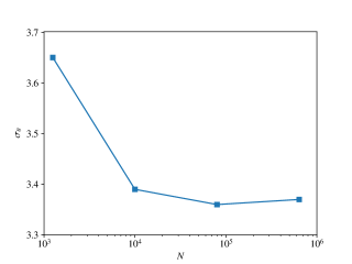
Figure 12: Convergence test of the shock-tube simulation for four different resolutions (1200, $10^{4}$, $8\times 10^{4}$ and $64\times 10^{4}$ cells) in a $10\times 1\times 1$ simulation box for a magnetic obliquity of $45^{\circ}$. The plot shows the standard deviation $\sigma_{\theta}$ of the magnetic obliquity vs. the number of cells $N$ used in the initial setup.

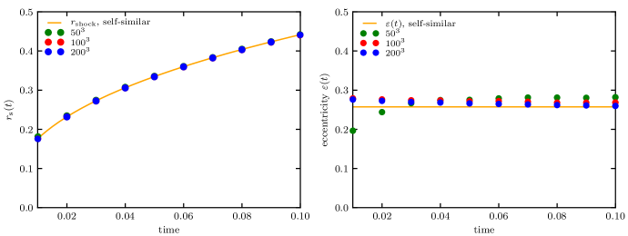
Figure 13: Convergence test for the Sedov-Taylor blast wave in the case of a homogeneous magnetic field and obliquity dependent CR acceleration with three different grid resolutions: $50^{3},100^{3}$ and $200^{3}$. The left panel shows the time evolution of the average shock radius while the right panel shows the time evolution of the eccentricity of the oblate explosion. Except for early times ($t<0.02$) the radius already converges for a simulation with $50^{3}$ cells. In contrast, the eccentricity converges only at a resolution of $200^{3}$ grid cells.

Here, we perform numerical convergence tests of our shock-tube and the Sedov-Taylor setups with a homogeneous magnetic field (see Sections 2 and 3, respectively). First, we asses the convergence of the accuracy with which we recover the magnetic obliquity in our simulations. We use several simulation outputs to measure the obliquity distribution, which follows a Gaussian, independent of resolution. Figure 12 shows the Gaussian standard deviation of the obliquity as a function of grid resolution, featuring 1200, $10^{4}$, $8\times 10^{4}$ and $64\times 10^{4}$ cells in our elongated shock tube setup ($10\times 1\times 1$). We notice that the standard deviation $\sigma_{\theta}$ decreases from $1200$ to $10^{4}$ cells and levels off for better resolved simulations, indicating convergence for measuring the magnetic obliquity for at least $10^{4}$ cells or equivalently $10^{3}$ cells per individual three-dimensional unit. To assess the numerical convergence of our ellipsoidal Sedov-Taylor problems with obliquity dependent CR acceleration, we perform simulations with $50^{3},100^{3}$ and $200^{3}$ grid cells. The results are reported in Fig. 13. The time evolution of the average shock radius (shown in the left panel) already converges for a $50^{3}$ simulation except for the first two points. We derive the radius of our self-similar solution with equation (17) using an average efficiency value taken from the $200^{3}$ simulation. Contrarily, the time evolution of the eccentricity of the oblate explosion (shown in the right panel) converges much slower and converges on our theoretical eccentricity at a resolution of $200^{3}$ cells. The self-similar solution of the eccentricity is constructed by fitting a Sedov-Taylor solution of the shock evolution to the data of the $200^{3}$ simulation in the parallel and perpendicular regions (as defined in Sect. 3.2).

Appendix B Details of the Sedov-Taylor solution

The Sedov-Taylor similarity solution makes two fundamental assumptions: (i) it assumes that the explosion was sufficiently long ago so that the initial conditions do not impact the solution and (ii) that the explosion expands into a medium of negligible pressure (or temperature). For these assumptions, the solution describes a strong spherical shock wave whose position only depends on the injected energy and the density of the ambient medium (Sedov, 1959; Taylor, 1950). These assumptions still hold when including a magnetic field that is flux-frozen into the gas. We follow the derivation by Landau & Lifshitz (1966) and only state the starting point and relevant definitions that are necessary to understand our final novel analytical expression of the self-similar parameter $\alpha$ in equation (13).

The velocity of the shock wave relative to the background gas at rest is given by (equation 13)

$$u_{1}=\dfrac{\mathrm{d}r_{\mathrm{s}}(t)}{\mathrm{d}t}=\dfrac{2r_{\mathrm{s}}(t)}{5t}=\dfrac{2}{5}\left(\dfrac{E_{1}}{\alpha\rho_{1}t^{3}}\right)^{1/5}.$$ (32)

Using the Rankine-Hugoniot expressions in the limit of strong shocks, the gas pressure $P_{2}$, mass density $\rho_{2}$ and velocity $v_{2}=u_{1}-u_{2}$ in the post-shock rest frame can be expressed in terms of the shock velocity $u_{1}$:

$$v_{2} = \dfrac{2u_{1}}{\gamma+1},$$ (33)

$$\rho_{2} = \dfrac{\gamma+1}{\gamma-1}\rho_{1},$$ (34)

$$P_{2} = \dfrac{2\rho_{1}u_{1}^{2}}{\gamma+1}.$$ (35)

To determine the gas flow in the region behind the shock, we introduce dimensionless variables $V,G,Z$ for the gas velocity $v$, density $\rho$ and the squared sound velocity $c^{2}$, respectively:

$$v = \dfrac{2r}{5t}\,V,$$ (36)

$$\rho = \rho_{1}G,$$ (37)

$$c^{2} = \dfrac{4r^{2}}{25t^{2}}\,Z.$$ (38)

These parameters are functions of the dimensionless variable

$$\xi=\dfrac{r}{r_{\mathrm{s}}(t)}=r\left(\dfrac{\alpha\rho_{1}}{E_{1}t^{2}}\right)^{1/5}.$$ (39)

Using these dimensionless quantities the conservation of energy can be expressed in terms of $Z$ and as an implicit function of $\xi$ through $V(\xi)$ (Landau & Lifshitz, 1966):

$$Z=\dfrac{\gamma(\gamma-1)(1-V)V^{2}}{2(\gamma V-1)}.$$ (40)

Following Landau & Lifshitz (1966), we arrive at the following set of equations:

$$\xi^{5}=\left[\dfrac{1}{2}(\gamma+1)V\right]^{-2} \left\{\dfrac{\gamma+1}{7-\gamma}[5-(3\gamma-1)V]\right\}^{\nu_{1}}$$ (41)

$$\times\left[\dfrac{\gamma+1}{\gamma-1}(\gamma V-1)\right]^{\nu_{2}},$$

$$G=\dfrac{\gamma+1}{\gamma-1}\left[\dfrac{\gamma+1}{\gamma-1}(\gamma V-1)\right]^{\nu_{3}} \left\{\dfrac{\gamma+1}{7-\gamma}[5-(3\gamma-1)V]\right\}^{\nu_{4}}$$ (42)

$$\times\left[\dfrac{\gamma+1}{\gamma-1}(1-V)\right]^{\nu_{5}}$$

with

$$\nu_{1} = -\dfrac{13\gamma^{2}-7\gamma+12}{(3\gamma-1)(2\gamma+1)},$$ (43)

$$\nu_{2} = \dfrac{5(\gamma-1)}{2\gamma+1},$$ (44)

$$\nu_{3} = \dfrac{3}{2\gamma+1},$$ (45)

$$\nu_{4} = -\dfrac{\nu_{1}}{2-\gamma},$$ (46)

$$\nu_{5} = -\dfrac{2}{2-\gamma}.$$ (47)

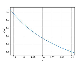
Figure 14: We show the self-similarity factor $\alpha$ of the Sedov-Taylor solution as a function of the ratio of specific heats $\gamma$.

The variable $\alpha$ as a function of the independent variable $\xi$ is determined by the condition

$$E_{1}=\int_{0}^{r_{\mathrm{s}}}\rho\left(\dfrac{1}{2}v^{2}+\dfrac{1}{\gamma-1}\dfrac{P}{\rho}\right)4\pi r^{2}\mathrm{d}r,$$ (48)

which states that the total energy of the gas is equal to the released energy of the original explosion. In terms of dimensionless quantities, this equation reads

$$\alpha=\dfrac{16}{25}\pi\int_{0}^{1}G(\xi)\left[\dfrac{1}{2}V^{2}(\xi)+\dfrac{Z(\xi)}{\gamma(\gamma-1)}\right]\xi^{4}\mathrm{d}\xi=\alpha(\gamma).$$ (49)

As $\gamma=c_{P}/c_{V}$ (where $c_{P}$ and $c_{V}$ are the specific heats at constant volume and pressure, respectively) we have $1<\gamma<2$. In our simulations we adopt values of $\gamma$ in the range $[4/3,5/3]$, such that $\alpha(\gamma)$ can be approximated with high precision, slightly modifying the formula used by Mihalas & Mihalas (1984):

$$\alpha(\gamma)\approx\dfrac{16}{75}\left[\dfrac{\pi(3\gamma-1)}{(\gamma-1)(\gamma+1)^{2}}-\dfrac{3}{8}\right],$$ (50)

which is accurate to within 0.8% and is shown in Fig. 14.

The dimensionless quantities defined via equations (36), (37) and (38) yield the implicit expressions for $v(r),\rho(r)$ and $P(r)$:

$$v(r) = \dfrac{1}{2}(\gamma+1)rV(r),$$ (51)

$$\rho(r) = G(r)\rho_{1},$$ (52)

$$P(r) = \dfrac{2\rho_{1}u^{2}_{1}}{\gamma+1}\left[\dfrac{1}{2}(\gamma+1)V\right]^{-6/5}\left[\dfrac{\gamma+1}{\gamma-1}\left(1-V\right)\right]^{-\nu_{5}+1}$$ (53)

$$\times\left\{\dfrac{\gamma+1}{7-\gamma}[5-(3\gamma-1)V]\right\}^{-\frac{\nu_{4}+2\nu_{1}}{5}}.$$

Appendix C Ellipsoidal reference frame

The radial unit vector of a spherical coordinate system is not perpendicular to an oblate surface except for the poles at $z=\pm b$, which would complicate the relation to the magnetic obliquity for a homogeneous magnetic field aligned with the $z$ axis. To simplify our computation of the magnetic obliquity on an oblate surface, we adopt the ellipsoid coordinate system. Here, the bisector of a tangent to point $P$ intersects the $z$ axis in $Q$, which varies according to the position of the point $P$ on the oblate surface (see Fig. 15). It assumes values from $0$ (for a point on the semi-major axis) to $-\infty$ (for a point on the semi-minor axis).

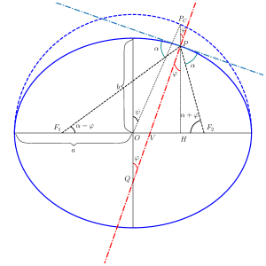
Figure 15: Elliptical section of an oblate that defines the ellipsoidal reference frame with the pseudo-azimuthal angle $\varphi$. The two focal points $F_{1}$ and $F_{2}$ determine a point $P$ on the surface of the ellipse. The tangent to that point (blue dash-dotted line) forms two equal angles $\alpha$ with the lines to the focii $\overline{PF_{1}}$ and $\overline{PF_{2}}$. Thus, the perpendicular to the tangent in $P$ (red dash-dotted line) intersects the $z$ axis in point $Q$, which varies with the position of $P$ and forms the desired angle $\varphi$.

A point $P$ on the ellipse has the property that the sum of distances from the two focal points $F_{1}$ and $F_{2}$ to $P$ is constant. A tangent to the ellipse in that point forms equal angles $\alpha$ with the two focal segments $\overline{F_{1}P}$ and $\overline{F_{2}P}$. Dropping the perpendicular to the tangent in $P$, by construction bisects the angle and intersects the $z$ axis in $Q$. The angle between this bisector and the $z$ axis defines the angle $\varphi$. Assuming a homogeneous magnetic field that is aligned with the $z$ axis, implies that the pseudo-azimuthal angle coincides with the magnetic obliquity, $\varphi=\theta$.

The point $P$ can be vertically projected onto a circumference in the point $P_{C}$, which forms an azimuthal angle $\psi$ with respect to the semi-minor axis $b$. The angle $\varphi$ is related to this angle via the following formula:

$$\tan\varphi=\dfrac{b}{a}\tan\psi.$$ (54)

Appendix D Sedov-Taylor solution of a dipole field

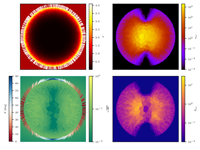
Figure 16: Sedov-Taylor blast wave with obliquity dependent CR acceleration expanding into a dipole magnetic field that is centered at point of the explosion and initially oriented horizontally. Quantities are shown at $t=0.1$ and are the same as in Fig. 5. Despite the different magnetic field morphology in comparison to the homogeneous case, the specific CR energy still exhibits a quadrupolar anisotropy, but with a broader region of CR production.

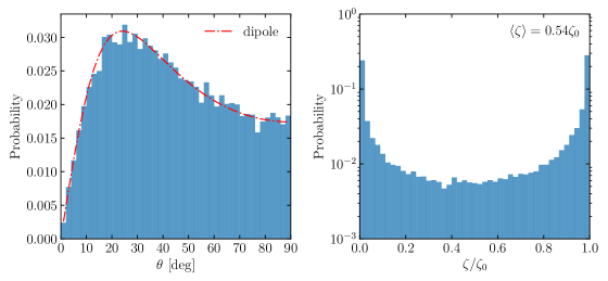
Figure 17: Probability distribution functions of the magnetic obliquity for the magnetic dipole case (left) and the resulting bimodal distribution for the acceleration efficiency (right). The theoretical distribution $f(\theta)$ of equation (60) (red dot-dashed line) compares nicely to our simulations.

As a last application, we study CR shock acceleration in the case of a magnetic dipole field with the dipole moment pointing in the positive $x$ direction. We chose the dipole configuration because it is expected to be the dominant magnetic configuration emerging from a non-rotating star at large distances and because of its self-similarity. While the magnitude of the magnetic field strength decreases as $r^{-3}$, where $r$ is distance from the source, the dipole field shows a constant magnetic obliquity at fixed latitude. This implies that the explosion encounters exactly the same replica of the magnetic field at different radii. We perform a $100^{3}$-cell simulation with an extremely low $\zeta_{0}=0.02$ to reduce the effect of CR pressure on the explosion shape and apply a Plummer-type softening length for $r\rightarrow 0$ to avoid magnetic divergence at the origin. The magnetic field in the polar regions is oriented mostly parallel to the shock normal, which results in efficient CR acceleration as the blast wave sweeps across it. The resulting quadrupolar CR morphology is shown in Fig. 16, resembling qualitative similarities to the homogeneous field case.

To analytically calculate the average efficiency we proceeded as follows. The normalised radial component of the magnetic dipole field is given by

$$\bm{\hat{b}}\mathchoice{\mskip 3.0mu\lower 0.86108pt\hbox{\scalebox{1.5}{$\cdot$}}\mskip 3.0mu}{\mskip 3.0mu\lower 0.86108pt\hbox{\scalebox{1.5}{$\cdot$}}\mskip 3.0mu}{\lower 1.29167pt\hbox{\scalebox{1.2}{$\cdot$}}}{\lower 1.29167pt\hbox{\scalebox{1.2}{$\cdot$}}}\bm{\hat{r}}=\dfrac{2\cos\vartheta}{\sqrt{1+3\cos^{2}\vartheta}},$$ (55)

where $\bm{\hat{r}}$ denotes a radial unit vector and $\vartheta$ is the azimuthal angle. Thus, the magnetic obliquity reads as

$$\theta(\vartheta)=\arccos(\bm{\hat{b}}\mathchoice{\mskip 3.0mu\lower 0.86108pt\hbox{\scalebox{1.5}{$\cdot$}}\mskip 3.0mu}{\mskip 3.0mu\lower 0.86108pt\hbox{\scalebox{1.5}{$\cdot$}}\mskip 3.0mu}{\lower 1.29167pt\hbox{\scalebox{1.2}{$\cdot$}}}{\lower 1.29167pt\hbox{\scalebox{1.2}{$\cdot$}}}\bm{\hat{r}})=\arccos\left(\dfrac{2\cos\vartheta}{\sqrt{1+3\cos^{2}\vartheta}}\right).$$ (56)

Capitalizing on the symmetry of both hemispheres, we calculate the average efficiency,

$$\langle\zeta\rangle=\int_{0}^{\pi/2}\zeta[\theta(\vartheta)]\sin\vartheta\ \mathrm{d}\vartheta=0.55\zeta_{0}.$$ (57)

Note that the result is considerably larger in comparison to our previously discussed case of CR acceleration in a turbulent field.

In Fig. 17 we show the obliquity distribution for a dipole field. To analytically predict this distribution, we invert equation (56) and obtain

$$\vartheta(\theta)=\arccos\left(\dfrac{\cos\theta}{\sqrt{4-3\cos^{2}\theta}}\right),\mbox{ with }\theta\in[0,\pi/2].$$ (58)

The distribution of magnetic obliquity in the case of a dipole field is obtained through a change of variables:

$$\sin\vartheta\ \mathrm{d}\vartheta=\sin[\vartheta(\theta)]\left(\dfrac{\mathrm{d}\vartheta}{\mathrm{d}\theta}\right)\mathrm{d}\theta=f(\theta)\mathrm{d}\theta,$$ (59)

where

$$f(\theta)=\dfrac{4\sin\theta}{(4-3\cos\theta)^{3/2}}.$$ (60)

This analytical result compares favorably to the simulations (see left-hand panel of Fig. 17). The simulated and theoretically expected average acceleration efficiencies agree within $2\%$ (for our $100^{3}$ cell simulation), demonstrating the accuracy of our numerical algorithms.

References

- Axford et al. (1977) Axford W. I., Leer E., Skadron G., 1977, International Cosmic Ray Conference, 11, 132
- Bell (1978) Bell A. R., 1978, MNRAS, 182, 147
- Bell (2004) Bell A. R., 2004, MNRAS, 353, 550
- Bell (2015) Bell A. R., 2015, MNRAS, 447, 2224
- Bell et al. (2013) Bell A. R., Schure K. M., Reville B., Giacinti G., 2013, MNRAS, 431, 415
- Beshley & Petruk (2012) Beshley V., Petruk O., 2012, MNRAS, 419, 1421
- Blandford & Ostriker (1978) Blandford R. D., Ostriker J. P., 1978, ApJ, 221, L29
- Bohdan et al. (2017) Bohdan A., Niemiec J., Kobzar O., Pohl M., 2017, ApJ, 847, 71
- Caprioli & Spitkovsky (2014) Caprioli D., Spitkovsky A., 2014, ApJ, 783, 91
- Caprioli et al. (2015) Caprioli D., Pop A.-R., Spitkovsky A., 2015, ApJ, 798, L28
- Castro et al. (2011) Castro D., Slane P., Patnaude D. J., Ellison D. C., 2011, ApJ, 734, 85
- Chevalier (1983) Chevalier R. A., 1983, ApJ, 272, 765
- Guo et al. (2014a) Guo X., Sironi L., Narayan R., 2014a, ApJ, 794, 153
- Guo et al. (2014b) Guo X., Sironi L., Narayan R., 2014b, ApJ, 797, 47
- HESS Collaboration et al. (2016) HESS Collaboration et al., 2016, Nature, 531, 476
- Kang & Ryu (2013) Kang H., Ryu D., 2013, ApJ, 764, 95
- Krymskii (1977) Krymskii G. F., 1977, Akademiia Nauk SSSR Doklady, 234, 1306
- Landau & Lifshitz (1966) Landau L. D., Lifshitz E. M., 1966, Hydrodynamik
- Lloyd (1982) Lloyd S. P., 1982, IEEE Trans. Information Theory, 28, 129
- Marcowith et al. (2016) Marcowith A., et al., 2016, Reports on Progress in Physics, 79, 046901
- Mihalas & Mihalas (1984) Mihalas D., Mihalas B. W., 1984, Foundations of radiation hydrodynamics
- Miyoshi & Kusano (2005) Miyoshi T., Kusano K., 2005, J. Comput. Phys., 208, 315
- Neronov (2017) Neronov A., 2017, Phys. Rev. Lett., 119
- Pakmor & Springel (2013) Pakmor R., Springel V., 2013, MNRAS, 432, 176
- Pakmor et al. (2011) Pakmor R., Bauer A., Springel V., 2011, MNRAS, 418, 1392
- Pakmor et al. (2016) Pakmor R., Springel V., Bauer A., Mocz P., Munoz D. J., Ohlmann S. T., Schaal K., Zhu C., 2016, MNRAS, 455, 1134
- Park et al. (2015) Park J., Caprioli D., Spitkovsky A., 2015, Physical Review Letters, 114, 085003
- Pfrommer et al. (2017a) Pfrommer C., Pakmor R., Schaal K., Simpson C. M., Springel V., 2017a, MNRAS, 465, 4500
- Pfrommer et al. (2017b) Pfrommer C., Pakmor R., Simpson C. M., Springel V., 2017b, ApJ, 847, L13
- Powell et al. (1999) Powell K. G., Roe P. L., Linde T. J., Gombosi T. I., De Zeeuw D. L., 1999, J. Comput. Phys., 154, 284
- Reynolds (2008) Reynolds S. P., 2008, ARA&A, 46, 89
- Sarkar et al. (2015) Sarkar K. C., Nath B. B., Sharma P., 2015, MNRAS, 453, 3827
- Schaal & Springel (2015) Schaal K., Springel V., 2015, MNRAS, 446, 3992
- Sedov (1959) Sedov L. I., 1959, Similarity and Dimensional Methods in Mechanics
- Springel (2010) Springel V., 2010, MNRAS, 401, 791
- Taylor (1950) Taylor G., 1950, Proceedings of the Royal Society of London Series A, 201, 159
- Yang et al. (2017) Yang R.-z., de Oña Wilhelmi E., Aharonian F., 2017, preprint, (arXiv:1710.02803)
- van Marle et al. (2015) van Marle A. J., Meliani Z., Marcowith A., 2015, A&A, 584, A49