Spin Polarized Non-Relativistic Fermions in 1+1 Dimensions

Abstract

We study by Monte Carlo methods the thermodynamics of a spin polarized gas of non-relativistic fermions in 1+1 dimensions. The main result of this work is that our action suffers no significant sign problem for any spin polarization in the region relevant for dilute degenerate fermi gases. This lack of sign problem allows us to study attractive spin polarized fermions non-perturbatively at spin polarizations not previously explored. For some parameters values we verify results previously obtained by methods which include an uncontrolled step like complex Langevin and/or analytical continuation from imaginary chemical potential. For others, larger values of the polarization, we deviate from these previous results.

I Introduction

Strongly coupled dilute fermi gases are rich systems which stand at the crossroads of various fields of physics. In the realm of nuclear physics, it is believed that the properties of dilute fermi gases with large scattering lengths are related to the properties of neutron rich matter at the edge of a neutron star Carlson et al. (2003). In the context of core collapse supernovae, the dynamic properties of dilute neutron gases must be analyzed to understand the propagation of energy which drive the explosion Burrows et al. (2006); Bedaque et al. (2018). In the atomic physics community, dilute fermi gases at unitarity have been studied to in the context of the BEC-BCS crossover Zwerger (2012). Spin polarizing these gases adds a layer of richness to observable phenomena. For instance, unequal density for the two spin states may either lead to an instability of Cooper pairing Bedaque et al. (2003) or the formation of the exotic superconducting phase predicted by Larkin, Ovchinnikov, Fulde, and Ferrell Fulde and Ferrell (1964); Larkin and Ovchinnikov (1965), characterized by formation of Cooper pairs which spontaneously break translation invariance. High magnetic fields in neutron stars can destroy $S$-wave pairing in neutron matter through spin polarization, which has observable consequences on spectroscopic data gathered from rapidly rotating neutron stars Stein et al. (2016).

All these systems are strongly coupled and to investigate their properties requires non-perturbative methods. One general approach to analyzing strongly coupled systems with controllable systematic uncertainties are ab initio Monte Carlo calculations. This approach runs into difficulties for spin imbalanced non-relativistic systems due to the sign problem which causes statistical uncertainties to grow exponentially as the thermodynamic and zero temperature limits are taken. The source of the sign problem in fermionic systems are sign oscillations of the fermion determinant.

A few suggestions for dealing with the sign problem in spin polarized non-relativistic systems have been put forward in the past. One is to compute observables at imaginary chemical potential, which renders the fermion determinant positive definite, and hence eliminates the sign problem and analytically continue them to real chemical potentials. The process of analytic continuation from restricted, noise data is necessarily done with the help of an ansatz which introduces an uncontrolled source of error. Still, mean field results suggest that interesting features of the phase diagram lie within the region where extrapolation works Braun et al. (2013). For the one dimensional case, this avenue has been tested numerically Loheac et al. (2015). Another approach is the Complex Langevin method where the configuration space is augmented by complexifying the field variables and stochastic process is used to sample configurations in this complex space Rammelmüller et al. (2017); Loheac et al. (2018). Complex Langevin has also been used to analyze non-relativistic fermions with a mass imbalance, which is a system that also suffers from the sign problem Rammelmüller et al. (2017). The potential problem of complex Langevin calculations is that it may converge to the wrong result and/or lead to runaway solutions Aarts and James (2010); Mollgaard and Splittorff (2013); Aarts et al. (2011). The problem of runaway solutions was cleverly taken care, in the one-dimensional non-relativistic case, by modifying the action with an extra term whose strength is taken to zero at the end Drut (2017); Loheac and Drut (2017). It would be important to verify and validate this method by independent means.

In the present work we show that, the sign problem is very mild in the parameter region investigated using other methods Loheac et al. (2015); Rammelmüller et al. (2017) and direct investigations of the polarized systems can be performed. We study the simple case of fermions interacting through an attractive s-wave interaction in $1+1$ dimensions, with an eye toward extending our work to atomic and nuclear systems 2+1 and 3+1 dimensions. Preliminary analysis indicate that the sign problem is also very mild in higher spatial dimensions as well.

This paper is organized as follows: In Section II we discuss the model and its lattice discretization. In Section III we describe the details of our Monte Carlo simulations. In Section IV we present the results of our simulations. Lastly, in Section V we summarize our findings and discusses future prospects.

II The Model

We study the thermodynamics of a dilute system of non-relativistic spin-1/2 fermions interacting via a contact interaction. The Hamiltonian of the system is

$$H=\int dx\,\left[\sum_{\sigma=\uparrow,\downarrow}\psi_{\sigma}^{\dagger}(x)\left(-\frac{\nabla^{2}}{2}\right)\psi_{\sigma}(x)-G\ n_{\uparrow}(x)n_{\downarrow}(x)\right]\,,$$ (1)

where $\sigma$ runs over the fermion polarizations and $n_{\sigma}(x)=\psi_{\sigma}^{\dagger}(x)\psi_{\sigma}(x)$ is the fermion density. We use non-relativistic natural units $\hbar=M=k_{B}=1$ with $M$ being the mass of the fermion. We take the interaction to be attractive so $G>0$. In one spatial dimension, the s-wave coupling is cutoff independent since fermion-fermion loops are ultraviolet finite. $G$ is related to the binding energy of the unique two-particle bound state by $E=-{G^{2}}/{4}$ (in the continuum, infinite volume limit).

The grand canonical partition function for the system can be written using the path integral formulation:

$$Z=\mathop{\hbox{Tr}}e^{-\beta(H-\sum_{\sigma}\mu_{\sigma}N_{\sigma})}=\int{D\psi D\psi^{\dagger}e^{-S[\psi,\psi^{\dagger}]}}\,,$$ (2)

with $N_{\sigma}=\int dx\,n_{\sigma}(x)$. In the path integral formulation the integrand involves the Euclidean action

$$S=\int_{0}^{\beta}\int{d\tau dx\Bigg{[}\sum_{\sigma}(\psi_{\sigma}^{\dagger}\partial_{\tau}\psi_{\sigma}-\psi_{\sigma}^{\dagger}\frac{\nabla^{2}}{2}\psi_{\sigma}-\mu_{\sigma}\psi_{\sigma}^{\dagger}\psi_{\sigma})-G(\psi_{\uparrow}^{\dagger}\psi_{\uparrow})(\psi_{\downarrow}^{\dagger}\psi_{\downarrow})\Bigg{]}}\,,$$ (3)

The chemical potentials are defined as $\mu_{\uparrow}=\mu+h$, $\mu_{\downarrow}=\mu-h$. $\mu$ controls the density of particles while the spin chemical potential $h$ controls the spin polarization. Note that in the path integral the fields $\psi$ are Grassman fields, but we use the same notation as the operator fields appearing in the Hamiltonian to keep the notation simple.

For numerical simulations the quartic fermion term associated with the contact interaction is transformed into a quadratic term via a Hubbard-Stratonovich transformation Hubbard (1959). The discretized action we start with is

$$\begin{split}S=&\frac{1}{\hat{g}}\sum_{x,t}{\Big{[}\cosh(A_{x,t})-1\Big{]}}+\sum_{\sigma;x,t}\Bigg{[}{\hat{\psi}^{\dagger}_{\sigma;x,t}\hat{\psi}_{\sigma;x,t}}-{\hat{\psi}^{\dagger}_{\sigma;x,t+1}\text{e}^{A_{x,t}+\hat{\mu}_{\sigma}}\hat{\psi}_{\sigma;x,t}}\\ &+\frac{\hat{\gamma}}{2}{{(\hat{\psi}^{\dagger}_{\sigma;x+1,t}-\hat{\psi}^{\dagger}_{\sigma;x,t})(\hat{\psi}_{\sigma;x+1,t}-\hat{\psi}_{\sigma;x,t})}}\Bigg{]}\end{split}$$ (4)

where $A_{xt}$ is a real, bosonic auxiliary field and $\hat{\mu}_{\sigma}=\hat{\mu}\pm\hat{h}$. All hatted quantities denote lattice quantities. The discretized action converges to the right continuum limit when

$$\begin{split}\mu\Delta t&=\frac{f_{1}}{f_{0}}\text{e}^{\hat{\mu}}\cosh\hat{h}-1\\ h\Delta t&=\frac{f_{1}}{f_{0}}\text{e}^{\hat{\mu}}\sinh\hat{h}\\ \frac{G\Delta t}{\Delta x}&=\left(\frac{f_{2}}{f_{0}}-\frac{f^{2}_{1}}{f^{2}_{0}}\right)e^{2\hat{\mu}}\\ \frac{\Delta t}{\Delta x^{2}}&=\hat{\gamma}\end{split}\,,\qquad\text{or inversely}\qquad\begin{split}&\hat{\gamma}=\Delta t/\Delta x^{2}\\ &\zeta=(\mu\Delta t+1)^{2}-(h\Delta t)^{2}\\ &\hat{h}={\rm arcsinh\,}(h\Delta t/\sqrt{\zeta})\\ &\frac{f_{1}^{2}}{f_{0}f_{2}}=\frac{\zeta}{\zeta+G\Delta t/\Delta x}(\text{solve for $\hat{g}$})\\ &\hat{\mu}=\log(\sqrt{\zeta}f_{0}/f_{1})\end{split}\,,$$ (5)

where

$$f_{\alpha}(\hat{g})\equiv\int_{-\infty}^{\infty}dA\exp\left(-\frac{\cosh A-1}{\hat{g}}+\alpha A\right).$$ (6)

The matching conditions above can be derived by integrating out the auxiliary fields using the relation

$$\begin{split}&\int_{-\infty}^{\infty}dA\exp\left(-\frac{\cosh A-1}{\hat{g}}\right)\,\exp[-\hat{\psi}^{\dagger}e^{A+\mu}\hat{\psi}]=\int_{-\infty}^{\infty}dA\exp\left(-\frac{\cosh A-1}{\hat{g}}\right)\,[1-\hat{\psi}^{\dagger}e^{A+\mu}\hat{\psi}+\frac{1}{2}(\hat{\psi}^{\dagger}e^{A+\mu}\hat{\psi})^{2}]\\ &\quad=f_{0}-f_{1}\hat{\psi}^{\dagger}e^{\mu}\hat{\psi}+\frac{1}{2}f_{2}(\hat{\psi}^{\dagger}e^{\mu}\hat{\psi})^{2}=f_{0}\exp\left[\frac{f_{1}}{f_{0}}\hat{\psi}^{\dagger}e^{\mu}\hat{\psi}+\left(\frac{f_{2}}{f_{0}}-\frac{f_{1}^{2}}{f_{0}^{2}}\right)\frac{1}{2}(\hat{\psi}^{\dagger}e^{\mu}\hat{\psi})^{2}\right]\,,\end{split}$$ (7)

and then take the continuum limit $\Delta t,\Delta x\to 0$. The continuum time and space limits can be taken separately. If we take the continuum time limit first we get the partition function for a discretized fermionic system with on-site interactions, an attractive version of the Hubbard model, with Hamiltonian

$$H_{\text{disc}}=\sum_{x}\left\{\sum_{\sigma}\left[\frac{1}{2\Delta x^{2}}(\hat{\psi}_{\sigma;x+1}^{\dagger}-\hat{\psi}_{\sigma;x}^{\dagger})(\hat{\psi}_{\sigma;x+1}-\hat{\psi}_{\sigma;x})-\mu_{\sigma}\hat{n}_{\sigma;x}\right]-\frac{G}{\Delta x}\hat{n}_{\uparrow,x}\hat{n}_{\downarrow,x}\right\}\,.$$ (8)

Note that above $\hat{\psi}$’s are operators normalized to satisfy the canonical commutation relations $\{\hat{\psi}_{\sigma;x}^{\dagger},\hat{\psi}_{\sigma^{\prime};x^{\prime}}\}=\delta_{\sigma\sigma^{\prime}}\delta_{xx^{\prime}}$. The discretized partition function converges linearly, as ${\cal O}(\Delta t)$, to the time continuum limit. We will show this explicitly and discuss how to improve the $\Delta\rightarrow 0$ convergence later. When taking the spatial continuum limit, the discretized Hamiltonian above contain errors of order $\Delta x^{2}$. In any case, the convergence rate does not change if we replace the matching conditions above with their first order approximation in the $\Delta t\to 0$ limit:

$$\hat{\gamma}=\frac{\Delta t}{\Delta x^{2}}\,,\quad\hat{h}=h\Delta t\,,\quad\hat{\mu}=\mu\Delta t-\frac{G\Delta t}{2\Delta x}\,,\quad\text{and}\quad\hat{g}=\frac{G\Delta t}{\Delta x}\,.$$ (9)

We will use these matching conditions for our simulations.

III Numerical method

The fermionic part of the action is quadratic in the fields and we can compute analytically the integral over the fermionic variables. The partition function resulting is then

$$Z=\int\prod_{x,t}dA_{x,t}\,e^{-S_{g}(A)}\det D(A)\,,$$ (10)

where $S_{g}(A)=\sum_{x,t}(\cosh A_{x,t}-1)/\hat{g}$ and $D(A)$ is the fermionic matrix appearing in Eq. 4. The matrix is block diagonal in spin space, that is $D_{\sigma xt,\sigma^{\prime}x^{\prime}t^{\prime}}=\delta_{\sigma\sigma^{\prime}}(D_{\sigma})_{xt,x^{\prime}t^{\prime}}$ with

$$\begin{split}&(D_{\sigma})_{xt,x^{\prime}t^{\prime}}=B_{xx^{\prime}}\delta_{tt^{\prime}}-e^{\hat{\mu}_{\sigma}}C_{xx^{\prime}}(A_{t})\delta_{t,t^{\prime}+1}\,,\\ &B_{xx^{\prime}}=(1+\hat{\gamma})\delta_{xx^{\prime}}-\frac{\hat{\gamma}}{2}(\delta_{x,x^{\prime}+1}+\delta_{x,x^{\prime}-1})\,,\qquad C(A_{t})_{xx^{\prime}}=\delta_{x,x^{\prime}}\text{e}^{A_{xt}}\,.\end{split}$$ (11)

Above, $A_{t}$ indicates the slice of the lattice field $A$ at time $t$. Note that the dependence on spin appears only as a factor multiplying the temporal hopping matrix $C$. Since the determinant is diagonal in spin space we have $\det D(A)=\det D_{\uparrow}(A)\det D_{\downarrow}(A)$. When $\hat{h}=0$ then $\mu_{\uparrow}=\mu_{\downarrow}$ and $\det D(A)=\det D_{\uparrow}(A)^{2}>0$, a positive quantity since $D_{\sigma}$’s are real matrices. For the spin polarized case, $\hat{h}\neq 0$, the determinant is no longer always positive raising the possibility of a sign problem. The sampling will then be done using the positive probability distribution

$$p_{\text{pq}}(A)=\frac{1}{Z}e^{-S_{g}(A)}|\det D(A)|\,.$$ (12)

The sign of the determinant is then included in the measured observable

$$\left\langle\mathcal{O}\right\rangle=\frac{\left\langle\mathcal{O}\,\text{sign}\,D\right\rangle_{\text{pq}}}{\left\langle\text{sign}\,D\right\rangle_{\text{pq}}}\,.$$ (13)

Above $\left\langle\cdot\right\rangle_{\text{pq}}$ indicates averages with respect to the phase quenched probability distribution $p_{\text{pq}}(A)$. An important observation in this paper is that for all simulations described here we did not encounter a negative determinant. This is not to say that there are no $A$ configurations that lead to negative determinants, but that for the parameter region used in this study the probability of such configurations is extremely small.

By for the most expensive step of the calculation is the computation of the fermion determinant, so we have optimized its computation. The fermion matrix, when the entries corresponding to a time-slice are grouped together, has the following structure

$$D_{\sigma}=\begin{bmatrix}B&0&\dots&e^{\hat{\mu}_{\sigma}}C(A_{N_{t}-1})\\ -e^{\hat{\mu}_{\sigma}}C(A_{0})&B&\dots&0\\ \vdots&\ddots&\ddots&\vdots\\ 0&\dots&-e^{\hat{\mu}_{\sigma}}C(A_{N_{t}-2})&B\end{bmatrix}\,.$$ (14)

Using the sparsity of the temporal blocks, the calculation of the determinant $\det D_{\sigma}$ can be reduced to a smaller problem using Schur’s complement methods, similar to the procedure used for Wilson fermions in lattice QCD Alexandru and Wenger (2011) (note that a similar expression was derived earlier for the Hubbard model using operator methods Blankenbecler et al. (1981); White et al. (1989)). We have

$$\det D_{\sigma}=\det B^{N_{t}}\det(\mathbf{1}+e^{N_{t}\hat{\mu}_{\sigma}}B^{-1}C(A_{N_{t}-1})...B^{-1}C(A_{0}))\,.$$ (15)

The cost of calculating the fermion determinant is reduced from a complexity of ${\cal O}((N_{t}N_{x})^{3})$ to ${\cal O}(N_{t}N_{x}^{3})$. Further simplifications appear because the matrices $C(A)$ are diagonal, so their multiplications has only a cost linear in $N_{x}$ and because matrix $B$ does not depend on the fields $A$ and its determinant and inverse are calculated only once. For periodic boundary conditions the eigenvectors of $B$ are plane waves $(\psi_{k})_{x}=\exp(ikx)$ with $k$ an integral multiple of $2\pi/N_{x}$. The inverse is then

$$(B^{-1})_{xx^{\prime}}=\frac{1}{N_{x}}\sum_{k}\frac{1}{\lambda_{k}}\cos{k(x-x^{\prime})}\,,\quad\text{with}\quad\lambda_{k}=1+2\hat{\gamma}\sin^{2}(k_{x}/2)\,.$$ (16)

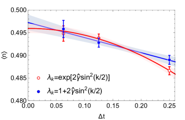
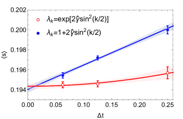
Figure 1: Continuum time limit for the density (left) and spin (right) at $\beta\mu=2.0$ and $\beta h=2.0$. The spatial lattice spacing is fixed to $\Delta x=1$ and the number of sites to $N_{x}=61$. The extrapolation is done with a quadratic correction for the exponentiated form and with a linear correction for the other case.

As it turns out the partition function in the reduced form as it appears in Eq. 15 is very similar to the one for the Hubbard model White et al. (1989): the fermionic contribution in given by a similar product of matrices with a diagonal matrix including the auxiliary field contribution and a non-diagonal matrix, similar to $B$, that encodes spatial hopping. The main difference is that the off-diagonal matrix is $\exp(\Delta tK)$, where $K_{xx^{\prime}}\propto\delta_{x,x^{\prime}+1}+\delta_{x,x^{\prime}-1}$ is the spatial hopping matrix, whereas for us $B\propto 1+\Delta tK$. The Trotter time discretization used for the Hubbard model has errors of the order ${\cal O}(\Delta t^{2})$ White et al. (1989); Fye (1986), whereas our discretization has errors ${\cal O}(\Delta t)$ (this can be seen by considering that the two discretizations differ at order $\Delta t^{2}$ for one step, but the full expression requires $\beta/\Delta t$ steps.) A simple way to improve our calculation is to replace the $B$ matrix above with the exponentiated expression. This amounts simply to replacing the eigenvalues in the precalculation of the inverse of the $B$ matrix with $\lambda_{k}=\exp[2\hat{\gamma}\sin^{2}(k/2)]$ rather than $1+2\hat{\gamma}\sin^{2}(k/2)$. In Fig. 1 we show the continuum time limit using the two versions of the $B$ matrix, for two observables used in this study. We see that they both converge to the same limit, but the exponentiated version of the $B$ matrix converges faster, as expected.

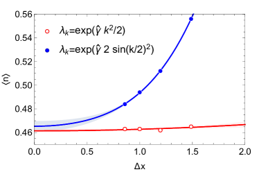
Figure 2: Left: Continuum limit in space for the density at $\beta\mu=2.0$ and $\beta h=2.0$. The spatial lattice size is fixed to $L=61$. The extrapolation is done with a quadratic correction for the continuum dispersion form and with a quadratic plus quartic correction for the other case. Right: Thermodynamic limit for the density for $\beta\mu=2.0$ and $\beta h=2.0$.

In a similar vein, we can improve the behavior of the space continuum limit. Note that using the exponentiated form the eigenvalues of the $B$ matrix are $\lambda_{k}=\exp[2\hat{\gamma}\sin^{2}(k/2)]=\exp[\Delta t\hat{E}(k)]$ with $\hat{E}(k)$ the lattice dispersion relations which for small $k$ approximate the continuum ones $\hat{E}(k)\approx E(k)=(k/\Delta x)^{2}/2$. A simple improvement is to replace the dispersion relations in the eigenvalues with the continuum form, that is use $\lambda_{k}=\exp[\gamma k^{2}/2]$ with $k\in\{-\lfloor N_{x}/2\rfloor,\ldots,-1,0,1,\ldots,\lfloor N_{x}/2\rfloor\}$ in units of $2\pi/N_{x}$. In the left panel of Fig. 2 we show the continuum limit using the lattice and continuum dispersion relations. We can see that both converge to the same limit but the convergence is much faster for the calculation using the continuum dispersion relation. In the right panel of Fig. 2 we look at the thermodynamic limit. For this calculation we use the exponentiated form for the $B$ matrix and the continuum dispersion relations. We set $\Delta t=0.025$ and $\Delta x=1.0$ which produce values indistinguishable from the continuum limit at the level of stochastic error bars. We see that for this rather high density, the thermodynamic limit can be achieved with $L\geq 20$.

Our simulations were carried out using two sampling methods: a straightforward Metropolis sampling and Hybrid Molecular Dynamics (HMC). In the Metropolis method we generated new fields by proposing global random changes in the auxiliary field $A$, with the shift at every point limited by a step-size parameter adjusted to produce an acceptance rate around 50%. The probability distribution used in the accept/reject step is the one given in Eq. 12, with $\det D$ as given by Eq. 15 but with the matrix $B$ replaced with $\tilde{B}$ associated with the continuum dispersion relations

$${\tilde{B}}_{xx^{\prime}}=\frac{1}{N_{x}}\sum_{k}{\lambda_{k}}\cos{k(x-x^{\prime})}\,,\quad\text{with}\quad\lambda_{k}=\exp[\gamma k^{2}/2]\,.$$ (17)

For the HMC we have to evolve the field $A$ and its conjugate momentum $\pi$ according to the canonical equations of motion induced by the Hamiltonian $H=\sum_{xt}\pi_{xt}^{2}/2+S(A)$. The force term is derived from the integrand in Eq. 12

$$\dot{\pi}_{xt}=-\frac{\partial S}{\partial A_{xt}}=-\frac{1}{\hat{g}}\sinh A_{xt}+\sum_{\sigma}[1-(1+e^{N_{t}\hat{\mu}_{\sigma}}U_{t}(A))^{-1}]_{x;x}\,,$$ (18)

where $U_{t}(A)={\tilde{B}}^{-1}C(A_{t+N_{t}-1})...{\tilde{B}}^{-1}C(A_{t})$. The HMC sampling requires the determinant to be positive, but this seems to be the case in all our simulations; we will discuss this point below in more detail. We carried out simulations for many different parameters using both Metropolis and HMC sampling and the results agreed in all cases.

A point to note is that in the evaluation of matrix $U_{t}(A)$ for large $N_{t}$, required for both Metropolis and HMC sampling, the product matrix $U$ exhibits numerical instabilities. This problem is encountered in Hubbard model simulations and it was found that the instability can be overcome by using a factorization of the intermediate results White et al. (1989): the product is split into subproducts of matrices that can be computed directly intermixed with factorizations. A similar instability appears when computing the force term for the HMC algorithm: A simple optimization is to compute $[1+\exp(N_{t}\hat{\mu}_{\sigma})U_{0}(A)]^{-1}$ and then evaluate the other time-slices using the property

$$[1+e^{N_{t}\hat{\mu}_{\sigma}}U_{t}(A)]^{-1}=[C(A_{t-1})^{-1}\tilde{B}]^{-1}[1+e^{N_{t}\hat{\mu}_{\sigma}}U_{t-1}(A)]^{-1}[C(A_{t-1})^{-1}\tilde{B}]\,.$$ (19)

The matrices $C(A_{t})$ are diagonal and trivial to invert and the $\tilde{B}$ matrix and its inverse are precomputed. This iteration can be used safely for a small number of time-slices, but for large $N_{t}$ we need to recompute $U_{t}(A)$ from time to time. In our runs we found that subproducts of up to 20 matrices can be performed safely when using double precision arithmetic.

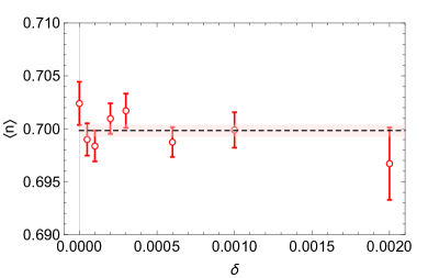
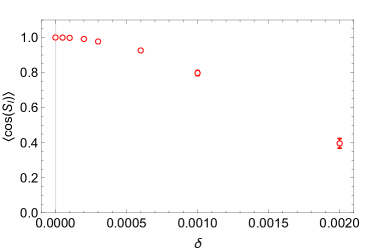
Figure 3: Results for the shifted integration contour $A_{xt}\rightarrow A_{xt}+i\delta$ as a function of $\delta$. On the left we have the density and in the right panel we plot the value of the phase average $\left\langle\cos(\mathop{\hbox{Im}}S)\right\rangle$. The horizontal line in the density plot corresponds to a common fit to all data points.

One final issue to discuss for our numerical simulations is the possibility of trapping in the positive determinant region of the configuration space. This issue arises even for non-polarized simulations where $\det D=(\det D_{\uparrow})^{2}$ and the determinant is positive. While the determinant is positive, the individual spin determinant $\det D_{\uparrow}$ changes sign and the positive and negative regions are separated by borders where the determinant is zero. Since both Metropolis and HMC sampling rely on small (or smooth) changes in the configuration, the edges of the same sign regions act as potential barriers and it is possible that the simulation becomes trapped. This lack of ergodicity was studied in the context of Hubbard model for both Metropolis sampling Scalettar et al. (1991) and HMC Beyl et al. (2018). For polarized systems the same-sign regions of $\det D_{\uparrow}$ and $\det D_{\downarrow}$ are not identical: as the polarization increases the borders between these regions are broadened and the determinant $\det D$ has fluctuating signs. Since we do not see any sign fluctuation, we believe that the probability distribution we sample has small (almost vanishing) overlap with these regions.

As a further test, we changed the integration manifold to avoid trapping, a method inspired by our work on thimbles Alexandru et al. (2016). The basic idea is that a generalization of the Cauchy theorem guarantees that the path integral remains unchanged for rather large set of deformations of the integration domain in the complex field space. We consider here a shift of the integration domain in the imaginary direction, which amount to adding a constant imaginary component to each field variable: $A_{xt}\to A_{xt}+i\delta$. While the integral remains the same, the integrand becomes complex and exhibits phase fluctuations. For small shifts, the fluctuations will be mild except close to the regions where the determinant changes sign. As we move away from the real integration domain the potential barriers associated with the zero determinant are lowered, removing trapping, but the sign fluctuations become larger. If the results are biased by trapping we should see a change in the value of the observables as we vary the imaginary shift $\delta$ away from zero. In Fig. 3 we plot the density and the average phase as a function of $\delta$ for one ensemble. The parameters used for this ensemble are $G=1/\sqrt{8}$, $L=61$ as for the other tests, but we move to lower temperature $\beta=8$ and higher densities and polarizations $\beta\mu=4$ and $\beta h=4$ as trapping is expected to appear more readily at low temperature and high densities. The lattice parameters are set to $\Delta x=1$ and $\Delta t=1/20$. We see that the density remains unchanged as we vary $\delta$ while the sign fluctuations become significant. The spin density is also unaffected by the shift. We conclude that it is unlikely that our simulations are trapped.

IV Results

The observables that we focus on here are the number and spin density:

$$\left\langle n\right\rangle=\left\langle n_{\uparrow}+n_{\downarrow}\right\rangle=\frac{1}{\beta L}\left\langle D^{-1}\frac{\partial D}{\partial\hat{\mu}}\right\rangle\quad\text{and}\quad\left\langle s\right\rangle=\left\langle n_{\uparrow}-n_{\downarrow}\right\rangle=\frac{1}{\beta L}\left\langle D^{-1}\frac{\partial D}{\partial\hat{h}}\right\rangle\,,$$ (20)

where the average is taken over Monte Carlo configurations. For our simulations we set $G=1/\sqrt{8}$ and $\beta=8$. The results presented are computed using $\Delta x=1$ and $\Delta t=1/8$ which are indistinguishable from the continuum results at the level of the error-bars (see Fig. 1 and Fig. 2). The volume is set to $L=61$ which is close to the thermodynamic limit. We set the parameters to these values to compare our results with those from imaginary polarization studies Loheac et al. (2015) and complex Langevin Drut (2017). All of our results are computed using 500 statistically independent measurements.

Our main result is presented in Fig. 4: for three values of $\beta\mu$ at $-2.0$, $0.0$, $2.0$ we sweep the spin chemical potential between $0\leq\beta h\leq 4.5$. In addition to our data, we also include in Fig. 4 the result of analytically continuing the results of calculations performed at imaginary chemical potential, a study carried out in Loheac et al. (2015). One finds at small polarization reasonable agreement between our method and analytic continuation, however at large polarization there is clear disagreement. The imaginary polarization method is expected to fail for large polarizations, when $\beta h\gtrsim\pi$, but we see large deviations for polarizations as small as $\beta h\gtrsim 2$. This may invalidate the expectations that interesting features of the phase diagram lie in the region where analitycal continuation is reliable Braun et al. (2013).

In Fig. 5 we compared our results with analytical continuation and the complex Langevin methods Drut (2017). We use a polarization of $\beta h=2$ and focus on the low chemical potential region where there seems to be a tension between the analytical continuation and the complex Langevin results. In this region our results seem to agree at low density with the imaginary-polarization method but as we increase the density the results seem to agree better with complex Langevin results. Since we do not have error estimates for the other methods, we cannot make a sharp statement.

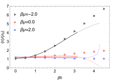
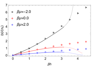
Figure 4: Density (left) and spin (right) normalized by the non-polarized density of the free fermi gas $n_{0}(\beta,\mu)$. The continuous lines show the results obtained in Loheac et al. (2015) by an analytic continuation from imaginary spin chemical potential. This method is expected to work well for $\beta h\leq\pi$, the region indicated by solid lines, but it quickly becomes unreliable as we move to higher polarizations, as we can see by comparing our results with the dotted lines.

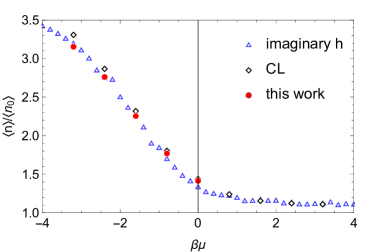
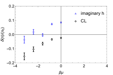
Figure 5: Our results for the density compared with results from analytical continuation from imaginary polarization Loheac et al. (2015) and complex Langevin simulations Drut (2017). The parameters for these simulations are $G=1/\sqrt{8}$, $\beta=8$, and $\beta h=2.0$. The right panel indicates the difference between our results and the other methods. The error-bars indicate the statistical uncertainties of our results since we did not have information about the error bars on the results from the other approaches.

V Conclusions

We study using Monte Carlo methods the physics of a system composed of two species of fermions in one spatial dimension, including unbalanced systems with unequal densities of the two species where a sign problem exists. We find that the sign problem is extremely mild for a vast range of parameters corresponding to densities small compared to the lattice cutoff scale which is the relevant parameters region for the continuum limit. This is in contrast to the parameter values corresponding to densities close to half-filling (but not exactly equal to it), relevant to the physics of the Hubbard model, where a severe sign problem occurs. The simulations in this work were carried out at $G=1/\sqrt{8}$, but we also find no negative determinants in simulations with couplings as high as $G=4/\sqrt{8}$ and it’s possible that even higher couplings have mild sign problems.

The range of density and spin studied in this work is wide. For some parameter values we are able to compare our results to previous calculations using the complex Langevin or the imaginary chemical potential methods. Detailed comparisons are not possible as the published results lack proper error bars but the general lesson is that out calculations are very close to the complex Langevin results (lending credence to its convergence to the right result) and agree with the imaginary chemical potential results at small enough asymmetries. For larger asymmetries our results are very different from the imaginary chemical potential ones. This is hardly surprising giving the nature of the analytic continuation from imaginary to real chemical potentials.

One potential problem with our calculations is the possibility that the Monte Carlo chain is trapped in a region of positive determinants. Besides producing the wrong result this would give the false impression that the sign problem is milder that it is in reality. Many pieces of evidence were offered to argue against that. The first is that calculations done with the Hybrid Monte Carlo method (more prone to trapping) agrees with the one done with the Metropolis algorithm (which is not likely to be trapped). We also used ideas from our work on the “thimble” approach to perform a calculation of the path integral not over the real variables, but over a hyperplane slightly shifted on the imaginary direction. Since now the determinants are complex the regions with opposite signs of the determinant are not separated by a repulsive barrier where the determinant vanishes. We observed no difference in the results. Finally, the agreement with other methods for parameter values where these methods are more reliable lend further confidence in our calculation.

It is unclear at this point whether similar methods can be easily extended to higher dimensional systems. Work in this direction is being pursued and results will appear elsewhere.

VI Acknowledgments

We gratefully acknowledge Joaquín E. Drut and Andrew C. Loheac for helpful comments on the manuscript and discussions. A.A. is supported in part by the National Science Foundation CAREER grant PHY-1151648 and by U.S. DOE Grant No.DE-FG02-95ER40907. P.B. and N.C.W. are supported by U.S. Department of Energy under Contract No. DE-FG02-93ER-40762. A.A. gratefully acknowledges the hospitality of the Physics Department at the University of Maryland where part of this work was carried out. P.B. and N.C.W gratefully acknowledge the hospitality of the Physics Department of The George Washington University where part of this work was carried out.

References

- Carlson et al. (2003) J. Carlson, S.-Y. Chang, V. R. Pandharipande, and K. E. Schmidt, in The Monte Carlo Method in the Physical Sciences, American Institute of Physics Conference Series, Vol. 690, edited by J. E. Gubernatis (2003) pp. 184–191.
- Burrows et al. (2006) A. Burrows, S. Reddy, and T. A. Thompson, Nucl. Phys. A777, 356 (2006), arXiv:astro-ph/0404432 [astro-ph] .
- Bedaque et al. (2018) P. F. Bedaque, S. Reddy, S. Sen, and N. C. Warrington, (2018), arXiv:1801.07077 [nucl-th] .
- Zwerger (2012) W. Zwerger, ed., The BCS-BEC Crossover and the Unitary Fermi Gas (Springer, Berlin, Heidelberg, 2012).
- Bedaque et al. (2003) P. F. Bedaque, H. Caldas, and G. Rupak, Phys. Rev. Lett. 91, 247002 (2003), arXiv:cond-mat/0306694 [cond-mat] .
- Fulde and Ferrell (1964) P. Fulde and R. A. Ferrell, Phys. Rev. 135, A550 (1964).
- Larkin and Ovchinnikov (1965) A. I. Larkin and Y. N. Ovchinnikov, Soviet Phys. JETP 20 (1965).
- Stein et al. (2016) M. Stein, A. Sedrakian, X.-G. Huang, and J. W. Clark, Phys. Rev. C 93, 015802 (2016).
- Braun et al. (2013) J. Braun, J.-W. Chen, J. Deng, J. E. Drut, B. Friman, C.-T. Ma, and Y.-D. Tsai, Phys. Rev. Lett. 110, 130404 (2013), arXiv:1209.3319 [cond-mat.stat-mech] .
- Loheac et al. (2015) A. C. Loheac, J. Braun, J. E. Drut, and D. Roscher, Phys. Rev. A 92, 063609 (2015).
- Rammelmüller et al. (2017) L. Rammelmüller, J. E. Drut, and J. Braun, in 19th International Conference on Recent Progress in Many-Body Theories (RPMBT19) Pohang, Korea, June 25-30, 2017 (2017) arXiv:1710.11421 [cond-mat.quant-gas] .
- Loheac et al. (2018) A. C. Loheac, J. Braun, and J. E. Drut, Proceedings, 35th International Symposium on Lattice Field Theory (Lattice 2017): Granada, Spain, June 18-24, 2017, EPJ Web Conf. 175, 03007 (2018), arXiv:1710.05020 [cond-mat.quant-gas] .
- Rammelmüller et al. (2017) L. Rammelmüller, W. J. Porter, J. E. Drut, and J. Braun, Phys. Rev. D 96, 094506 (2017).
- Aarts and James (2010) G. Aarts and F. A. James, JHEP 08, 020 (2010), arXiv:1005.3468 [hep-lat] .
- Mollgaard and Splittorff (2013) A. Mollgaard and K. Splittorff, Phys. Rev. D 88, 116007 (2013).
- Aarts et al. (2011) G. Aarts, F. A. James, E. Seiler, and I.-O. Stamatescu, Eur. Phys. J. C71, 1756 (2011), arXiv:1101.3270 [hep-lat] .
- Drut (2017) J. E. Drut, in 19th International Conference on Recent Progress in Many-Body Theories (RPMBT19) Pohang, Korea, June 25-30, 2017 (2017) arXiv:1710.10176 [cond-mat.quant-gas] .
- Loheac and Drut (2017) A. C. Loheac and J. E. Drut, Phys. Rev. D 95, 094502 (2017).
- Hubbard (1959) J. Hubbard, Phys. Rev. Lett. 3, 77 (1959).
- Alexandru and Wenger (2011) A. Alexandru and U. Wenger, Phys.Rev. D83, 034502 (2011), arXiv:1009.2197 [hep-lat] .
- Blankenbecler et al. (1981) R. Blankenbecler, D. J. Scalapino, and R. L. Sugar, Phys. Rev. D24, 2278 (1981).
- White et al. (1989) S. R. White, D. J. Scalapino, R. L. Sugar, E. Y. Loh, J. E. Gubernatis, and R. T. Scalettar, Phys. Rev. B40, 506 (1989).
- Fye (1986) R. M. Fye, Phys. Rev. B 33, 6271 (1986).
- Scalettar et al. (1991) R. T. Scalettar, R. M. Noack, and R. R. P. Singh, Phys. Rev. B 44, 10502 (1991).
- Beyl et al. (2018) S. Beyl, F. Goth, and F. F. Assaad, Phys. Rev. B 97, 085144 (2018).
- Alexandru et al. (2016) A. Alexandru, G. Basar, P. F. Bedaque, G. W. Ridgway, and N. C. Warrington, JHEP 05, 053 (2016), arXiv:1512.08764 [hep-lat] .