Adversarial Semantic Alignment for Improved Image Captions
Abstract
In this paper we study image captioning as a conditional GAN training, proposing both a context-aware LSTM captioner and co-attentive discriminator, which enforces semantic alignment between images and captions. We empirically focus on the viability of two training methods: Self-critical Sequence Training (SCST) and Gumbel Straight-Through (ST) and demonstrate that SCST shows more stable gradient behavior and improved results over Gumbel ST, even without accessing discriminator gradients directly. We also address the problem of automatic evaluation for captioning models and introduce a new semantic score, and show its correlation to human judgement. As an evaluation paradigm, we argue that an important criterion for a captioner is the ability to generalize to compositions of objects that do not usually co-occur together. To this end, we introduce a small captioned Out of Context (OOC) test set. The OOC set, combined with our semantic score, are the proposed new diagnosis tools for the captioning community. When evaluated on OOC and MS-COCO benchmarks, we show that SCST-based training has a strong performance in both semantic score and human evaluation, promising to be a valuable new approach for efficient discrete GAN training.
1 Introduction
Significant progress has been made on the task of generating image descriptions using neural image captioning. Early systems were traditionally trained using cross-entropy (CE) loss minimization [27, 11, 28]. Later, reinforcement learning techniques [22, 23, 14] based on policy gradient methods, e.g., REINFORCE, were introduced to directly optimize the -gram matching metrics such as CIDEr [26], BLEU4 [20] or SPICE [1]. Along a similar idea, [23] introduced Self-critical Sequence Training (SCST), a light-weight variant of REINFORCE, which produced state of the art image captioning results using CIDEr as an optimization metric. Although optimizing the above automatic metrics might be a promising direction to take, these metrics unfortunately miss an essential part of the semantic alignment between image and caption. They do not provide a way to promote naturalness of the language, e.g., as measured by a Turing test, so that the machine-generated text becomes indistinguishable from the text created by humans.
To address the problem of diversity and naturalness, image captioning has recently been explored in the framework of GANs [6]. The main idea is to train a discriminator to detect a signal on the misalignment between an image and a generated sentence, while the generator (captioner) can use this signal to improve its text generation mechanism to better align the caption with a given image. Due to the discrete nature of text generation, GAN training remains challenging and has been generally tackled with either reinforcement learning techniques [29, 3, 8, 21, 4] or by using the Gumbel softmax relaxation [9], for example, as in [25, 12].
Despite these impressive advances, image captioning is far from being a solved task. It still is a challenge to satisfactory bridge a semantic gap between image and caption, and to produce diverse, creative and human-like captions. The current captioning systems also suffer from a dataset bias: the models overfit to common objects co-occurring in common context, and they struggle to generalize to scenes where the same objects appear in unseen contexts. Although the recent advances of applying GANs for image captioning to promote human-like captions is a very promising direction, the discrete nature of the text generation process makes it challenging to train such systems. The results in [4, 25] are encouraging but the proposed solutions are still complex and computationally expensive. Moreover, the recent work of [2] showed that the task of text generation for the current discrete GAN models is still challenging, many times producing unsatisfactory results, and therefore requires new approaches and methods. Finally, evaluation of image captioning using automated metrics such as CIDEr, BLEU4, etc. is still unsatisfactory since simple -gram matching, that does not reference the image, remains inadequate and sometimes misleading for scoring diverse and descriptive captions.
In this paper, we propose to address the above issues by accomplishing the following three main objectives: 1) Architectural and algorithmic improvements: We propose a novel GAN-based framework for image captioning that enables better language composition and more accurate compositional alignment of image and text (Section 2.1), as well as a light-weight and efficient approach for discrete GAN training based on SCST (Section 2.2). 2) Automated scoring metric: We propose the semantic score, which enables quantitative automatic evaluation of caption quality and its alignment to the image across multiple models (Section 3). 3) Diagnostic dataset: Finally, we introduce the Out of Context (OOC) test set which is a quick and useful diagnostic tool for checking a model’s generalization to out of context scenes (Section 3).
2 Adversarial Caption Generation
In this Section we present our novel captioner and the discriminator models. We employ SCST for discrete GAN optimization and compare it with the approach based on the Gumbel trick. Our experiments (Section 4) show that SCST obtains better results, even though it does not directly access the discriminator gradients.
2.1 Compositional Captioner and Discriminator
Here we introduce an image captioning model with attention that we call context aware captioning based on [15]. This allows the captioner to compose sentences based on fragments of observed visual scenes in the training. Furthermore, we introduce a discriminator that scores the alignment between images and captions based on a co-attention model [16]. This gives the generator a signal on the semantic alignment and the compositional nature of visual scenes and language. We show in Section 4 that we obtain better results across evaluation metrics when using this co-attentive discriminator.
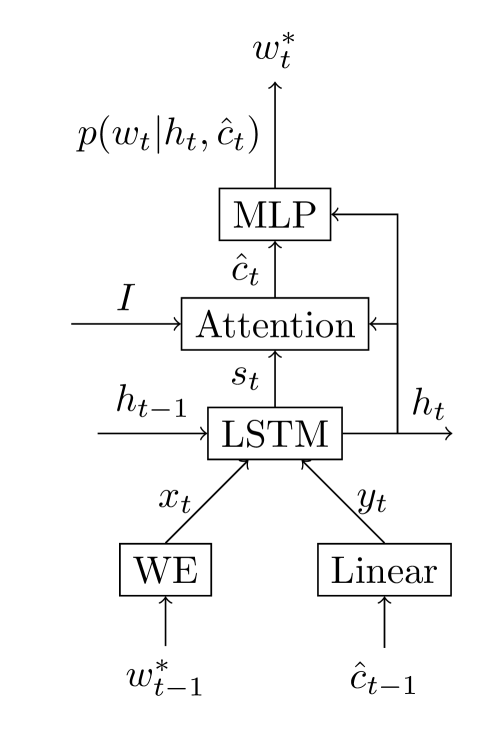
Context Aware Captioner . For caption generation, we use an LSTM with visual attention [28, 23] together with a visual sentinel [15] to give the LSTM a choice of attending to visual or textual cues. While [15] feeds only an average image feature to the LSTM at each step, we feed a mixture of image and visual sentinel features from the previous step to make the LSTM aware of the last attention context, as seen in Figure 1. We call it Context Aware Attention. This simple modification gives significant gains, as the captioner is now aware of the contextual information used in the past. As reported in Table 1, a captioner with an adaptive visual sentinel [15] gives 99.7 CIDEr vs. 103.3 for our Context Aware Attention on COCO validation set.
| Attention Model | CE | RL |
|---|---|---|
| Att2All [23] | 98.5 | 115.7 |
| Sentinel [15] | 99.7 | |
| Context Aware (ours) | 103.3 | 118.6 |
Co-attention Pooling Discriminator . The task of the discriminator is to score the similarity between an image and a caption. Previous works jointly embed the modalities at the similarity computation level, which we call late joint embedding, see Figure 2 (a). Instead, we propose to jointly embed image and caption in earlier stages using a co-attention model [16, 5] and compute similarity on the attentive pooled representation. We call this a Co-attention discriminator (Figure 2 (b)) and provide architectural details below.

(a) Joint-Embedding Discriminator (Joint-Emb) [4]

(b) Proposed Co-Attention Discriminator (Co-att)

Given a sentence composed of a sequence of words , the discriminator embeds each word using the LSTM (state dimension ) to get for , where . For image , we extract features , where (number of crops) and also embed them as , where , and , our image feature size. Following [16], we then compute a correlation between image and text using bilinear projection , . Matrix is used to compute co-attention weights of one modality conditioned on another:
where all new matrices are in . The above weights are used then to combine the word and image features: and for . Finally, the image-caption score is computed as (, discriminator parameters). In Section 4 we compare with the late joint embedding approach of [4, 25], where is the average spatial pooling of CNN features and the last state of LSTM. We refer to this discriminator as Joint-Emb and to ours as Co-att (see Figure 2).
2.2 Adversarial Training
In this Section we describe the details of the adversarial training of the discriminator and the captioner.
Training . Our discriminator is not only trained to distinguish real captions from fake (generated), but also to detect when images are coupled with random unrelated real sentences, thus forcing it to check not only the sentence composition but also the semantic relationship between image and caption. To accomplish this, we solve the following optimization problem: , where the loss
| (1) |
where is the real sentence, is sampled from generator (fake caption), and is a real but randomly picked caption.
Training . The generator is optimized to solve , where . The main difficulty is the discrete, non-differentiables nature of the problem. We propose to solve this issue by adopting SCST [23], a light-weight variant of the policy gradient method, and compare it to the Gumbel relaxation approach of [9].
Training with SCST. SCST [23] is a REINFORCE variant that uses the reward under the decoding algorithm as baseline. In this work, the decoding algorithm is a “greedy max”, selecting at each step the most probable word from . For a given image, a single sample of the generator is used to estimate the full sequence reward, where . Using SCST, the gradient is estimated as follows:
where is obtained using greedy max (see Figure 3). Note that the baseline does not change the expectation of the gradient but reduces the variance of the estimate.
Also, observe that the GAN training can be regularized with any NLP metric (such as CIDEr) to enforce closeness of the generated captions to the provided ground truth on the -gram level; the gradient then becomes:
There are two main advantages of SCST over other policy gradient methods used in the sequential GAN context: 1) The reward in SCST can be global at the sentence level and the training still succeeds. In other policy gradient methods, e.g., [4, 14], the reward needs to be defined at each word generation with the full sentence sampling, so that the discriminator needs to be evaluated times (sentence length). 2) In [4, 14, 8], many Monte-Carlo rollouts are needed to reduce variance of gradients, requiring many forward-passes through the generator. In contrast, due to a strong baseline, only a single sample estimate is enough in SCST.
Training : Gumbel Trick.
An alternative way to deal with the discreteness of the generator is by using Gumbel re-parameterization [9]. Define the soft samples , for (sentence length) and (vocabulary size) such that: where are samples from Gumbel distribution, is a temperature parameter. We experiment with the Gumbel Soft and Gumbel Straight-Through (Gumbel ST) approaches, recently used in [25, 12].
For Gumbel Soft, we use the soft samples as LSTM input at the next time step and in :
For Gumbel ST, we define one-hot encodings and approximate the gradients . To sample from we use the hard as LSTM input at the next time step and in , hence the gradient becomes:
Observe that this loss can be additionally regularized with Feature Matching (FM) as follows:
| (2) |
where is the ground truth caption corresponding to image , and and are co-attention image and sentence embeddings (as defined in Section 2.1). Feature matching enables us to incorporate more granular information from discriminator representations of the ground truth caption, similar to how SCST reward can be regularized with CIDEr, computed with a set of baseline captions.
3 Evaluation: Semantic Score and OOC Set
| COCO Test Set | OOC (Out of Context) | |||||||||||||||
| CIDEr | METEOR | Semantic | Vocabulary | CIDEr | METEOR | Semantic | Vocabulary | |||||||||
| Score | Coverage | Score | Coverage | |||||||||||||
| CE | 101.6 | 0.4 | 0.260 | .001 | 0.186 | .001 | 9.2 | 0.1 | 42.2 | 0.6 | 0.169 | .001 | 0.118 | .001 | 2.8 | 0.1 |
| CIDEr-RL | 116.1 | 0.2 | 0.269 | .000 | 0.184 | .001 | 5.1 | 0.1 | 45.0 | 0.6 | 0.170 | .003 | 0.117 | .002 | 2.1 | 0.0 |
| GAN1(SCST, Co-att, ) | 97.5 | 0.8 | 0.256 | .001 | 0.190 | .000 | 11.0 | 0.1 | 41.0 | 1.6 | 0.168 | .003 | 0.124 | .000 | 3.2 | 0.1 |
| GAN2(SCST, Co-att, CIDEr) | 111.1 | 0.7 | 0.271 | .002 | 0.192 | .000 | 7.3 | 0.2 | 45.8 | 0.9 | 0.173 | .001 | 0.122 | .002 | 2.8 | 0.1 |
| GAN3(SCST, Joint-Emb, ) | 97.1 | 1.2 | 0.256 | .002 | 0.188 | .000 | 11.2 | 0.1 | 41.8 | 1.6 | 0.167 | .002 | 0.122 | .001 | 3.3 | 0.0 |
| GAN4(SCST, Joint-Emb, CIDEr) | 108.2 | 4.9 | 0.267 | .004 | 0.190 | .000 | 8.3 | 1.6 | 45.4 | 1.4 | 0.173 | .002 | 0.122 | .003 | 2.8 | 0.2 |
| GAN5(Gumbel Soft, Co-att, ) | 93.6 | 3.3 | 0.253 | .007 | 0.187 | .002 | 11.1 | 1.2 | 38.3 | 3.7 | 0.164 | .006 | 0.121 | .004 | 3.3 | 0.3 |
| GAN6(Gumbel ST, Co-att, ) | 95.4 | 1.5 | 0.249 | .004 | 0.184 | .003 | 10.1 | 0.9 | 38.5 | 1.9 | 0.161 | .005 | 0.116 | .004 | 3.0 | 0.2 |
| GAN7(Gumbel ST, Co-att, FM) | 92.1 | 5.4 | 0.243 | .011 | 0.175 | .006 | 8.6 | 0.8 | 36.8 | 2.3 | 0.157 | .006 | 0.110 | .005 | 2.5 | 0.2 |
| CE∗ – ∗denotes non-attentional models | 87.6 | 1.2 | 0.242 | .001 | 0.175 | .002 | 9.9 | 0.8 | 32.0 | 0.4 | 0.152 | .002 | 0.103 | .002 | 2.6 | .1 |
| CIDEr-RL∗ | 100.4 | 7.9 | 0.253 | .006 | 0.173 | .002 | 6.8 | 1.4 | 33.4 | 1.4 | 0.154 | .003 | 0.101 | .003 | 2.1 | .2 |
| GAN1∗(SCST, Co-att, ) | 89.7 | 0.9 | 0.246 | .001 | 0.184 | .001 | 13.2 | 0.2 | 30.8 | 1.0 | 0.155 | .003 | 0.111 | .001 | 3.4 | 0.1 |
| GAN2∗(SCST, Co-att, CIDEr) | 103.1 | 0.5 | 0.261 | .001 | 0.183 | .001 | 7.1 | 0.2 | 33.7 | 1.9 | 0.157 | .001 | 0.108 | .001 | 2.7 | 0.1 |
| GAN3∗(SCST, Joint-Emb, ) | 90.7 | 0.1 | 0.248 | .001 | 0.181 | .001 | 12.9 | 0.1 | 30.8 | 2.1 | 0.153 | .002 | 0.108 | .001 | 3.5 | 0.1 |
| GAN4∗(SCST, Joint-Emb, CIDEr) | 102.7 | 0.4 | 0.260 | .001 | 0.182 | .001 | 7.7 | 0.1 | 33.3 | 2.4 | 0.157 | .004 | 0.106 | .000 | 2.7 | 0.1 |
| G-GAN [4] from Table 1 | 79.5 | – | 0.224 | – | – | – | – | – | – | – | – | – | – | – | – | – |
Semantic Score. Traditional automatic language metrics, such as CIDEr or BLEU4, are inadequate for evaluating GAN-based image caption models. As an early alternative, [4, 25] used GAN discriminator for evaluation, but this is not a fair comparison across models since the GAN generator was trained to maximize the discriminator likelihood. In order to enable automatic evaluation across models we propose the semantic score. Analogous to “Inception Score” [24] for image generation, leveraging a large pretrained classification network, the semantic score relies on a powerful model, trained with supervision, to heuristically evaluate caption quality and its alignment to the image. In Section 4 we show that our semantic score correlates well with human judgement across metrics, algorithms and test sets.
The semantic score is based on a Canonical Correlation Analysis (CCA) retrieval model [18] which brings the image into the scoring loop by training on the combination of COCO [13] and SBU [19] (1M images), ensuring a larger exposure of the score to diverse visual scenes and captions, and lowering the COCO dataset bias. The semantic score is a cosine similarity in CCA space based on a 15k dimension image embedding from resnet-101 [7], and a sentence embedding computed using a Hierarchical Kernel Sentence Embedding [18] based on word2vec [17]:
where and are caption and image embedding vectors, respectively; , , and are matrices obtained from CCA as described in details in [18]. Note that the use of word2vec allows the computation of scores for captions whose words fall outside of the COCO vocabulary. The computed score can be interpreted as a likelihood of the image given a caption, it also penalizes the sentences which mention non-existent attributes or objects. See Table 4 in Appendix A for examples.
Out of Context Set (OOC). An important property of the captioner is the ability to generalize to images with objects falling outside of their common contexts. In order to test the compositional and generalization properties to out-of-context scenes (see Figure 7 for an example), we expanded the original set of [10] (containing images) to a total of images and collected captions per image on Amazon MTurk. We call the resulting dataset the Out of Context (OOC) set. We note that although the size of OOC set is not large, its main purpose is to be a useful quick diagnostic tool rather than a traditional dataset. The evaluation on OOC is a good indicator of a captioner’s generalization: poor performance is a sign that the model is over-fitted to the training context. Improving OOC scores remains an open area for future work, and we plan to release the OOC set as well as the scripts for computing the semantic score.
4 Experiments
Experimental Setup. We evaluate our proposed method and the baselines on COCO dataset [13] (vocabulary size is 10096) using data splits from [11]: training set of 113k images with captions each, validation and test sets 5k each; as well as on the proposed OOC diagnostic set. Each image is encoded by a resnet-101 [7] without rescaling or cropping, followed by a spatial adaptive max-pooling to ensure a fixed size of 14142048. An attention mask is produced over the 1414 spatial locations, resulting in a spatially averaged 2048-dimension representation. LSTM hidden state, image, word, and attention embedding dimensions are fixed to 512 for all models. Before the GAN training, all the models are first pretrained with cross entropy (CE) loss. We report standard language evaluation metrics, the proposed semantic score, and the vocabulary coverage (percentage of vocabulary used at generation).
| COCO Test Set | OOC (Out of Context) | ||||||||
| CIDEr | METEOR | Semantic | Vocabulary | CIDEr | METEOR | Semantic | Vocabulary | ||
| Score | Coverage | Score | Coverage | ||||||
| (CE and RL Baselines) | Ens(CE) | 105.8 | 0.266 | 0.189 | 8.4 | 44.8 | 0.172 | 0.122 | 2.6 |
| Ens(CIDEr-RL) | 118.9 | 0.273 | 0.186 | 5.0 | 48.8 | 0.175 | 0.122 | 2.1 | |
| (SCST, Co-att, ) | Ens1(GAN1) | 102.6 | 0.262 | 0.195 | 9.9 | 44.8 | 0.172 | 0.129 | 3.0 |
| Ens2(GAN2) | 115.1 | 0.277 | 0.194 | 7.0 | 48.3 | 0.176 | 0.127 | 2.7 | |
| Ens12(GAN1,GAN2) | 113.2 | 0.274 | 0.195 | 7.3 | 49.9 | 0.178 | 0.129 | 2.6 | |
| (SCST, Joint-Emb, ) | Ens3(GAN3) | 109.8 | 0.270 | 0.193 | 8.5 | 48.5 | 0.175 | 0.127 | 2.8 |
| Ens4(GAN4) | 113.0 | 0.274 | 0.193 | 7.6 | 48.0 | 0.178 | 0.127 | 2.7 | |
| Ens34(GAN3,GAN4) | 111.1 | 0.271 | 0.193 | 8.1 | 50.1 | 0.177 | 0.127 | 2.8 | |
| (Gumbel , Co-att, ) | Ens5(GAN5) | 100.1 | 0.259 | 0.191 | 10.0 | 43.1 | 0.170 | 0.127 | 3.0 |
| Ens6(GAN6) | 99.6 | 0.253 | 0.187 | 9.3 | 41.0 | 0.165 | 0.122 | 2.8 | |
| Ens7(GAN7) | 100.2 | 0.254 | 0.180 | 7.8 | 38.9 | 0.164 | 0.113 | 2.3 | |
| Ens567(GAN5,GAN6,GAN7) | 103.2 | 0.258 | 0.188 | 8.7 | 41.8 | 0.164 | 0.121 | 2.7 | |
| (SCST+Gumbel Soft, Co-att, ) | Ens125(GAN1,GAN2,GAN5) | 112.4 | 0.273 | 0.195 | 7.7 | 49.8 | 0.179 | 0.129 | 2.7 |
Experimental Results. Table 2 presents results for both COCO and OOC datasets for two discriminator architectures (ours Co-att, and baseline Joint-Emb) for all training algorithms (SCST, Gumbel ST, and Gumbel Soft). For reference, we also include results for non-GANs captioners: CE (trained only with cross entropy) and CIDEr-RL (pretrained with CE, followed by SCST to optimize CIDEr), as well as results from non-attentional models. As expected, CIDEr-RL greatly improves the language metrics as compared to the CE model (from 101.6 to 116.1 CIDEr on COCO), but this also leads to a significant drop in the vocabulary coverage (from 9.2% to 5.1% for COCO), indicating that the -gram optimization can lead to vanilla sentences, discouraging style deviations from the ground truth captions. In the table, gan1 gan4 denote the GAN-based models, where we use SCST training (with or rewards) with either Co-att or Joint-Emb discriminators; and gan5 gan7 are the models trained with the Gumbel relaxation. From our extensive experiments we observed that SCST provides significantly more stable training of the models and better results as compared to Gumbel approaches, which often become unstable beyond 15 epochs and underperform SCST GANs on many evaluation metrics (see also Section E in Supplement for additional discussion on SCST vs. Gumbel).
It can noticed that SCST GAN models outperform CE and CIDEr-RL captioners on semantic score and vocabulary coverage for both COCO and OOC sets. The CIDEr regularization of SCST GAN additionally improves CIDEr and METEOR scores, and also results in the improvement of the semantic score (at the cost of some vocabulary coverage loss) as seen for gan1 vs. gan2 and gan3 vs. gan4. We also see that SCST GANs using our Co-att discriminator outperform their Joint-Emb [4] counterparts on every metric except vocabulary coverage (for COCO). We conclude that gan2, a CIDEr-regularized SCST with Co-att discriminator, is the model with the best overall performance on COCO and OOC sets.
For baselining, we also reproduced results from [4] with non-attentional generators (same architecture as in [4]). Non-attentional models are behind in all metrics, except for vocabulary coverage on both datasets. Interestingly, Co-att discriminators still provide better semantic scores than Joint-Emb despite non-attentional generators.
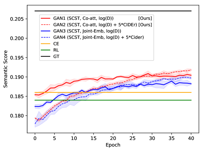
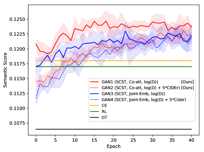
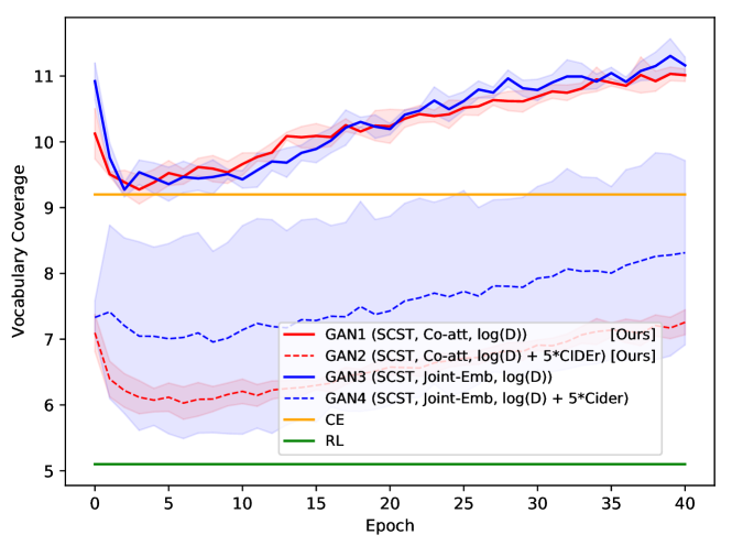
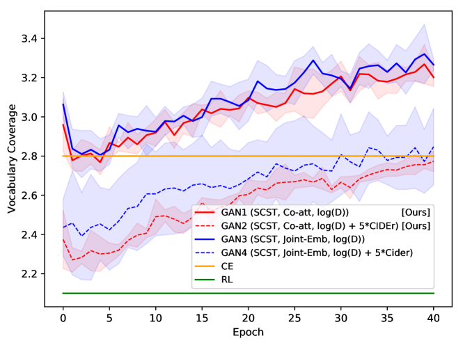
Figures 4 and 5 show the evolution of semantic scores and vocabulary coverage over the training epochs for gan1gan4, CE, CIDEr-RL and ground truth (GT) captions. Semantic scores increase steadily for all cost functions and discriminator architectures as the training sees more data. In Figure 4 (a), GAN models improve steadily over CE and RL, ultimately surpassing both of them mid-training. Moreover, Co-att GANs achieve higher semantic scores across the epochs than Joint-Emb GANs. For CIDEr-regularized SCST GANs, the same trend is observed but with a faster rate since the models start off worse than CE and RL. For OOC in Figure 4 (b), we see the same trend: Co-att GANs outperforming the other approaches. For COCO, GT semantic score is higher than the other models while the opposite is true for OOC. This may be caused by the vocabulary mismatch between OOC and the combination of COCO and SBU. Figures 4 and 5 show that the semantic score improvement of GAN-trained models correlates well with the vocabulary coverage increase for both COCO and OOC.
Ensemble Models. Table 3 presents results for ensemble models, where a caption is generated by first averaging the softmax scores from 4 different models before word selection. EnsCE and EnsRL ensemble CE and CIDEr-RL models. Similarly, Ens1Ens7 ensemble models from gan1gan7 respectively (Ensijk denotes an ensemble of gani, ganj, and gank). As compared to individual models, the ensembles show improved results on all metrics.
Ensembling SCST GANs provides the best results, reinforcing the conclusion that SCST is a superior method for a stable sequence GAN training. For comparison, we also computed SPICE [1] scores on COCO dataset: EnsCE 19.69, Ens12 20.64 (GAN Co-attention) and Ens34 20.46 (GAN Joint embedding from [4]), showing that SCST GAN training additionally improves the SPICE metric. Finally, we observe that underperformance of GANs over CIDEr-RL in terms of CIDEr is expected and explained by the fact that in GAN the objective is to make the sentences more descriptive and human-like, deviating from the vanilla ground truth captions, and this can potentially sacrifice the CIDEr performance. The generated captions are evaluated using the proposed semantic score which showed a good correlation with human judgment; see Figure 6 (c) for more details.
(c)|c|c||c|c|c|c|
 &
&

GAN: a row of motorcycles parked on the side of a street
CE: a row of motorcycles parked on a street
RL: a group of motorcycles parked in front of a building
GT: a bunch of motorcycles parked along the side of the street
GAN: two giraffes standing next to each other in a field
CE: two giraffes standing in a field with trees in the background
RL: a couple of giraffes standing next to each other
GT: two giraffe standing next to each other on a grassy field


GAN: a bus driving down a highway next to cars
CE: a bus driving down a street next to a car
RL: a bus driving down a highway with cars
GT: a bus traveling on a freeway next to other traffic
GAN: a stop sign with graffiti on it next to a street
CE: a stop sign with a sticker on it
RL: a stop sign with a street on top of it
GT: graffiti on a stop sign supporting the red sox
(c)|c|c||c|c|c|c|
 &
&

GAN: a bird is sitting on the floor next to a laptop
CE: a bird is sitting on the floor next to a laptop
RL: a bird sitting on the floor next to a laptop
GT: a bird on the ground with keys to the laptop are scattered on the floor
GAN: a black car parked on the side of the road
CE: a black car parked on the side of the road
RL: a black car parked on the side of a street
GT: a black car has gotten lodged atop a silver metal barrier on a roadway
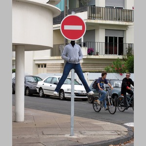
GAN: a man riding a bike next to a stop sign
CE: a man is walking down the street with a sign
RL: a man riding a bike down a street with a stop sign
GT: a person hangs from a street sign using the sign to cover their face
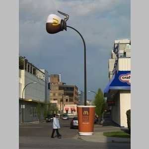
GAN: a person is standing in front of a coffee cup
CE: a person is walking down a street with a cup
RL: a cup of coffee sitting on top of a street
GT: a person looks up at a street light that is designed like a pot of coffee
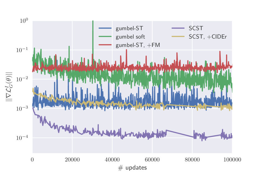
Gradient Analysis. Throughout the extensive experiments, the SCST showed to be a more stable approach for training discrete GAN nodels, achieving better results compared to Gumbel relaxation approaches. Figure 8 compares gradient behaviors during training for both techniques, showing that the SCST gradients have smaller average norm and variance across minibatches, confirming our conclusion.
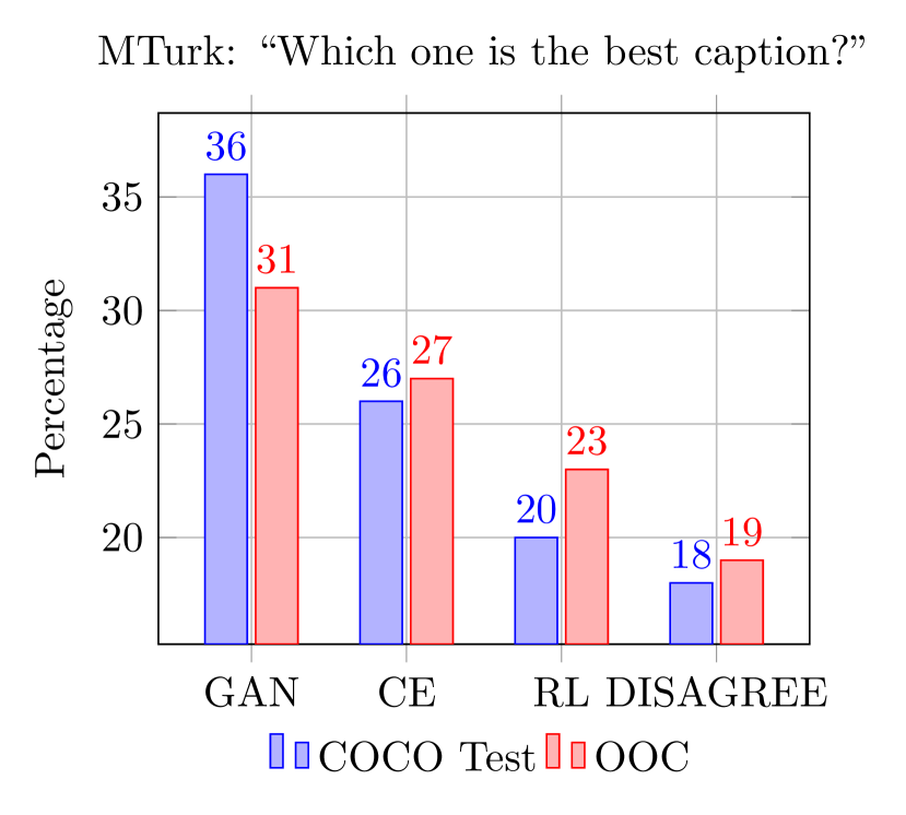
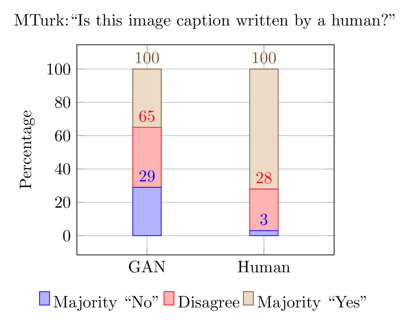
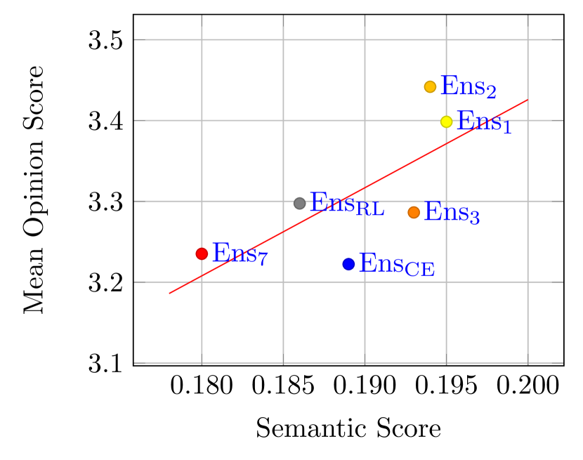
Human Evaluation. To validate the benefits of the semantic score, we also evaluate the image/caption pairs generated by several GAN ensembles, Ens and Ens on Amazon MTurk. For a given image, 5 workers are asked to rate each caption on the scale 1 to 5 (from which we computed mean opinion score (MOS)) as well as to select the best caption overall (additional details are given in Appendix D). Figure 6 (a) shows that GAN ensemble Ens2 scored higher than CE and CIDEr-RL on a majority vote, confirming that GAN training significantly improves perceived quality of the captions as compared to a more vanilla CE or RL-based captions. Figure 6 (b) gives Turing test results where the workers are asked if a given caption is human or machine-generated. Here, our GANs again performed well, demonstrating a good capacity at fooling humans. In Figure 6 (c) we show that MOS of human evaluations correlates well with our semantic score (see Table 7 in Appendix D for all scores). There is an overall trend (depicted with a red regression line for better visualization), where models that have higher semantic score are generally favored more by human evaluators. For example, Co-att SCST GANs Ens1 and Ens2 score the best semantic (resp. 0.195 and 0.194) and MOS scores (resp. 3.398 and 3.442) on COCO. We can see that the semantic score is able to capture semantic alignments pertinent to humans, validating it as a viable alternative to automatic language metrics and a proxy to human evaluation.
Finally, in Figure 7 we present a few examples of the captions for COCO and OOC sets. As compared to the traditional COCO dataset, the OOC images are difficult and illustrate the challenge for the automatic captioning in such settings. The difficulty is not only to correctly recognize the objects in the scene but also to compose a proper description, which is challenging even for humans (see row denoted by GT), as it takes more words to describe such unusual images.
5 Conclusion
In conlusion, we summarize the main messages from our study: 1) SCST training for sequence GAN is a promissing new approach that outperforms the Gumbel relaxation in terms of stability of training and the overall performance. 2) The modeling part in the captioner is crucial for generalization to out-of-context: we demonstrate that the non-attention captioners and discriminators – while still widely used – fail at generalizing to out of context, hinting at a memorization of the training set. Attentive captioners and discriminators succeed at composing on unseen visual scenes, as was demonstrated with our newly introduced OOC diagnostic set. 3) Human evaluation is still the gold standard for assessing the quality of GAN captioning. We showed that the introduced semantic score correlates well with the human judgement and can be a valuable addition to the existing evaluation toolbox for image captioning.
References
- [1] P. Anderson, B. Fernando, M. Johnson, and S. Gould. Spice: Semantic propositional image caption evaluation. In European Conference on Computer Vision, pages 382–398. Springer, 2016.
- [2] M. Caccia, L. Caccia, W. Fedus, H. Larochelle, J. Pineau, and L. Charlin. Language gans falling short. arXiv preprint arXiv:1811.02549, 2018.
- [3] T. Che, Y. Li, R. Zhang, D. R. Hjelm, W. Li, Y. Song, and Y. Bengio. Maximum-likelihood augmented discrete generative adversarial networks. arXiv:1702.07983, 2017.
- [4] B. Dai, D. Lin, R. Urtasun, and S. Fidler. Towards diverse and natural image descriptions via a conditional GAN. ICCV, 2017.
- [5] C. N. dos Santos, M. Tan, B. Xiang, and B. Zhou. Attentive pooling networks. Arxiv, abs/1602.03609, 2016.
- [6] I. Goodfellow, J. Pouget-Abadie, M. Mirza, B. Xu, D. Warde-Farley, S. Ozair, A. Courville, and Y. Bengio. Generative adversarial nets. In NIPS, 2014.
- [7] K. He, X. Zhang, S. Ren, and J. Sun. Deep residual learning for image recognition. In CVPR, 2016.
- [8] R. D. Hjelm, A. P. Jacob, T. Che, K. Cho, and Y. Bengio. Boundary-seeking generative adversarial networks. arXiv:1702.08431, 2017.
- [9] E. Jang, S. Gu, and B. Poole. Categorical reparameterization with gumbel-softmax. arXiv preprint arXiv:1611.01144, 2016.
- [10] M. Jinchoi, A. Torralba, and A. S. Willsky. Context models and out-of-context objects, 2012.
- [11] A. Karpathy and F.-F. Li. Deep visual-semantic alignments for generating image descriptions. In CVPR, 2015.
- [12] M. J. Kusner and J. M. Hernández-Lobato. Gans for sequences of discrete elements with the gumbel-softmax distribution. arXiv:1611.04051, 2016.
- [13] T. Lin, M. Maire, S. J. Belongie, L. D. Bourdev, R. B. Girshick, J. Hays, P. Perona, D. Ramanan, P. Dollár, and C. L. Zitnick. Microsoft COCO: common objects in context. EECV, 2014.
- [14] S. Liu, Z. Zhu, N. Ye, S. Guadarrama, and K. Murphy. Improved image captioning via policy gradient optimization of spider. In ICCV, 2017.
- [15] J. Lu, C. Xiong, D. Parikh, and R. Socher. Knowing when to look: Adaptive attention via a visual sentinel for image captioning. In CVPR, 2017.
- [16] J. Lu, J. Yang, D. Batra, and D. Parikh. Hierarchical question-image co-attention for visual question answering. In NIPS, 2016.
- [17] T. Mikolov, K. Chen, G. Corrado, and J. Dean. Efficient estimation of word representations in vector space. ArXiv, 2013.
- [18] Y. Mroueh, E. Marcheret, and V. Goel. Multimodal retrieval with asymmetrically weighted CCA and hierarchical kernel sentence embedding. ArXiv, 2016.
- [19] V. Ordonez, G. Kulkarni, and T. L. Berg. Im2text: Describing images using 1 million captioned photographs. In NIPS, 2011.
- [20] K. Papineni, S. Roukos, T. Ward, and W.-J. Zhu. Bleu: A method for automatic evaluation of machine translation. In ACL, 2002.
- [21] S. Rajeswar, S. Subramanian, F. Dutil, C. Pal, and A. Courville. Adversarial generation of natural language. arXiv:1705.10929, 2017.
- [22] M. Ranzato, S. Chopra, M. Auli, and W. Zaremba. Sequence level training with recurrent neural networks. ICLR, 2015.
- [23] S. J. Rennie, E. Marcheret, Y. Mroueh, J. Ross, and V. Goel. Self-critical sequence training for image captioning. In CVPR, 2017.
- [24] T. Salimans, I. Goodfellow, W. Zaremba, V. Cheung, A. Radford, and X. Chen. Improved techniques for training gans. NIPS, 2016.
- [25] R. Shetty, M. Rohrbach, L. A. Hendricks, M. Fritz, and B. Schiele. Speaking the same language: Matching machine to human captions by adversarial training. ICCV, 2017.
- [26] R. Vedantam, C. L. Zitnick, and D. Parikh. Cider: Consensus-based image description evaluation. In CVPR, 2015.
- [27] O. Vinyals, A. Toshev, S. Bengio, and D. Erhan. Show and tell: A neural image caption generator. CVPR, 2015.
- [28] K. Xu, J. Ba, R. Kiros, K. Cho, A. C. Courville, R. Salakhutdinov, R. S. Zemel, and Y. Bengio. Show, attend and tell: Neural image caption generation with visual attention. In ICML, 2015.
- [29] L. Yu, W. Zhang, J. Wang, and Y. Yu. Seqgan: Sequence generative adversarial nets with policy gradient. CoRR, abs/1609.05473, 2016.
Adversarial Semantic Alignment for Improved Image Captions
(Supplementary Material)
Pierre Dognin, Igor Melnyk, Youssef Mroueh, Jerret Ross & Tom Sercu
IBM Research, Yorktown Heights, NY
Appendix A Semantic Score
Semantic scores was first introduced int the context of image retrieval where it achieves state of the art performance [18]. Some examples of the properties of semantic scores are given in Table 4.
| COCO validation image | Set | Semantic | Captions |
| Score | |||
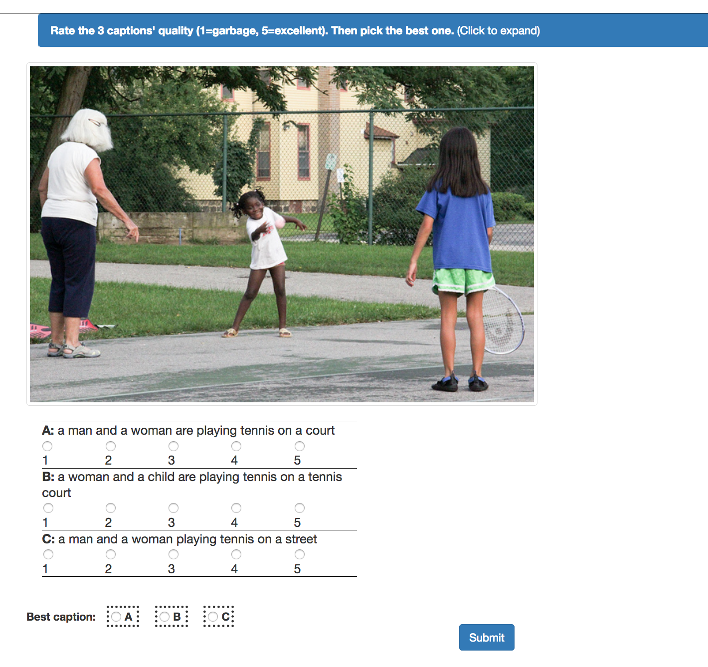
![[Uncaptioned image]](/html/1805.00063/assets/images/COCO_val2014_000000215906.jpg) |
Set A | 0.181052 | female tennis player reaches back to swing at the ball |
| 0.210224 | a woman on a court swinging a racket at a ball | ||
| 0.181592 | a woman in a gray top is playing tennis | ||
| 0.251200 | the woman is playing tennis on the court | ||
| 0.145646 | a woman prepares to hit a tennis ball with a racket | ||
| Set B | 0.008990 | a clear refrigerator is stocked up with food | |
| 0.005519 | a store freezer is shown with food inside | ||
| -0.014052 | a refrigerated display case is full of dairy groceries | ||
| 0.011076 | a close up of a commercial refrigerator with food | ||
| -0.029001 | a large cooler with glass doors containing mostly dairy products | ||
| Set C | 0.054441 | a giraffe reaches back to swing at the ball | |
| 0.123822 | female tennis player reaches back to swing at the boat | ||
| 0.152860 | male tennis player reaches back to swing at the ball | ||
| 0.067289 | female football player reaches back to swing at the ball | ||
| Set D | 0.152860 | male tennis player reaches back to swing at the ball | |
| 0.164755 | female tennis fan reaches back to swing at the ball | ||
| 0.152524 | female tennis player looks back to swing at the ball | ||
| 0.100098 | female flute player reaches back to swing at the ball | ||
| Set E | 0.114010 | female tennis player swing ball | |
| 0.031566 | female player swing ball | ||
| 0.084016 | tennis player swing ball | ||
| 0.115490 | tennis player ball | ||
| 0.092226 | tennis player | ||
| -0.044019 | tennis | ||
| -0.001948 | ball ball ball ball |
Appendix B Experimental Results: Complete Tables
We report here CIDEr, BLEU4, ROUGEL, METEOR, semantic scores, and vocabulary coverage for all models mentioned in this work, both COCO and OOC sets. Table 5 presents all GAN results as average ( standard deviation) over 4 models with different random seeds. Table 6 presents all our ensemble results.
| COCO Test Set | ||||||||||||
| CIDEr | BLEU4 | ROUGEL | METEOR | Semantic | Vocabulary | |||||||
| Score | Coverage | |||||||||||
| CE | 101.6 | 0.4 | 0.312 | .001 | 0.542 | .001 | 0.260 | .001 | 0.186 | .001 | 9.2 | 0.1 |
| CIDEr-RL | 116.1 | 0.2 | 0.350 | .003 | 0.562 | .001 | 0.269 | .000 | 0.184 | .001 | 5.1 | 0.1 |
| GAN1(SCST, Co-att, ) | 97.5 | 0.8 | 0.294 | .002 | 0.532 | .001 | 0.256 | .001 | 0.190 | .000 | 11.0 | 0.1 |
| GAN2(SCST, Co-att, CIDEr) | 111.1 | 0.7 | 0.330 | .004 | 0.555 | .002 | 0.271 | .002 | 0.192 | .000 | 7.3 | 0.2 |
| GAN3(SCST, Joint-Emb, ) | 97.1 | 1.2 | 0.287 | .005 | 0.530 | .002 | 0.256 | .002 | 0.188 | .000 | 11.2 | 0.1 |
| GAN4(SCST, Joint-Emb, CIDEr) | 108.2 | 4.9 | 0.325 | .017 | 0.551 | .008 | 0.267 | .004 | 0.190 | .000 | 8.3 | 1.6 |
| GAN5(Gumbel Soft, Co-att, ) | 93.6 | 3.3 | 0.282 | .015 | 0.524 | .007 | 0.253 | .007 | 0.187 | .002 | 11.1 | 1.2 |
| GAN6(Gumbel ST, Co-att, ) | 95.4 | 1.5 | 0.298 | .009 | 0.531 | .005 | 0.249 | .004 | 0.184 | .003 | 10.1 | 0.9 |
| GAN7(Gumbel ST, Co-att, FM) | 92.1 | 5.4 | 0.289 | .020 | 0.523 | .015 | 0.243 | .011 | 0.175 | .006 | 8.6 | 0.8 |
| G-GAN [4] from Table 1 | 79.5 | 0.207 | 0.475 | 0.224 | – | – | ||||||
| CE∗ – ∗ for non-attentional models | 87.6 | 1.2 | 0.275 | .003 | 0.516 | .003 | 0.242 | .001 | 0.175 | .002 | 9.9 | 0.8 |
| CIDEr-RL∗ | 100.4 | 7.9 | 0.305 | .018 | 0.536 | .010 | 0.253 | .006 | 0.173 | .002 | 6.8 | 1.4 |
| GAN1∗(SCST, Co-att, ) | 89.7 | 0.9 | 0.276 | .000 | 0.518 | .001 | 0.246 | .001 | 0.184 | .001 | 13.2 | 0.2 |
| GAN2∗(SCST, Co-att, CIDEr) | 103.1 | 0.5 | 0.311 | .003 | 0.542 | .001 | 0.261 | .001 | 0.183 | .001 | 7.1 | 0.2 |
| GAN3∗(SCST, Joint-Emb, ) | 90.7 | 0.1 | 0.277 | .002 | 0.520 | .000 | 0.248 | .001 | 0.181 | .001 | 12.9 | 0.1 |
| GAN4∗(SCST, Joint-Emb, CIDEr) | 102.7 | 0.4 | 0.315 | .000 | 0.542 | .000 | 0.260 | .001 | 0.182 | .001 | 7.7 | 0.1 |
| OOC (Out of Context) | ||||||||||||
| CIDEr | BLEU4 | ROUGEL | METEOR | Semantic | Vocabulary | |||||||
| Score | Coverage | |||||||||||
| CE | 42.2 | 0.6 | 0.168 | .005 | 0.413 | .003 | 0.169 | .001 | 0.118 | .001 | 2.8 | 0.1 |
| CIDEr-RL | 45.0 | 0.6 | 0.177 | .002 | 0.417 | .004 | 0.170 | .003 | 0.117 | .002 | 2.1 | 0.0 |
| GAN1(SCST, Co-att, ) | 41.0 | 1.6 | 0.161 | .013 | 0.406 | .006 | 0.168 | .003 | 0.124 | .000 | 3.2 | 0.1 |
| GAN2(SCST, Co-att, CIDEr) | 45.8 | 0.9 | 0.179 | .014 | 0.417 | .005 | 0.173 | .001 | 0.122 | .002 | 2.8 | 0.1 |
| GAN3(SCST, Joint-Emb, ) | 41.8 | 1.6 | 0.162 | .006 | 0.404 | .006 | 0.167 | .002 | 0.122 | .001 | 3.3 | 0.0 |
| GAN4(SCST, Joint-Emb, CIDEr) | 45.4 | 1.4 | 0.180 | .011 | 0.418 | .005 | 0.173 | .002 | 0.122 | .003 | 2.8 | 0.2 |
| GAN5(gumbel soft, Co-att, ) | 38.3 | 3.7 | 0.154 | .020 | 0.406 | .006 | 0.164 | .006 | 0.121 | .004 | 3.3 | 0.3 |
| GAN6(gumbel-ST, Co-att, ) | 38.5 | 1.9 | 0.148 | .005 | 0.407 | .004 | 0.161 | .005 | 0.116 | .004 | 3.0 | 0.2 |
| GAN7(gumbel-ST, Co-att, +FM) | 36.8 | 2.3 | 0.154 | .012 | 0.396 | .009 | 0.157 | .006 | 0.110 | .005 | 2.5 | 0.2 |
| CE∗ | 32.0 | 0.4 | 0.132 | .007 | 0.392 | .002 | 0.152 | .002 | 0.103 | .002 | 2.6 | .1 |
| CIDEr-RL∗ | 33.4 | 1.4 | 0.145 | .009 | 0.394 | .006 | 0.154 | .003 | 0.101 | .003 | 2.1 | .2 |
| GAN1∗(SCST, Co-att, ) | 30.8 | 1.0 | 0.127 | .001 | 0.383 | .006 | 0.155 | .003 | 0.111 | .001 | 3.4 | 0.1 |
| GAN2∗(SCST, Co-att, CIDEr) | 33.7 | 1.9 | 0.145 | .011 | 0.391 | .004 | 0.157 | .001 | 0.108 | .001 | 2.7 | 0.1 |
| GAN3∗(SCST, Joint-Emb, ) | 30.8 | 2.1 | 0.126 | .009 | 0.380 | .004 | 0.153 | .002 | 0.108 | .001 | 3.5 | 0.1 |
| GAN4∗(SCST, Joint-Emb, CIDEr) | 33.3 | 2.4 | 0.144 | .016 | 0.391 | .006 | 0.157 | .004 | 0.106 | .000 | 2.7 | 0.1 |
| COCO Test Set | |||||||||||||
| CIDEr | BLEU4 | ROUGEL | METEOR | Semantic | Vocabulary | ||||||||
| Score | Coverage | ||||||||||||
| (CE and RL Baselines) | Ens(CE) | 105.8 | 0.327 | 0.553 | 0.266 | 0.189 | 8.4 | ||||||
| Ens(CIDEr-RL) | 118.9 | 0.359 | 0.568 | 0.273 | 0.186 | 5.0 | |||||||
| (SCST, Co-att, ) | Ens1(GAN1) | 102.6 | 0.314 | 0.543 | 0.262 | 0.195 | 9.9 | ||||||
| Ens2(GAN2) | 115.1 | 0.347 | 0.566 | 0.277 | 0.194 | 7.0 | |||||||
| Ens12(GAN1,GAN2) | 113.2 | 0.344 | 0.564 | 0.274 | 0.195 | 7.3 | |||||||
| (SCST, Joint-Emb, ) | Ens3(GAN3) | 109.8 | 0.331 | 0.556 | 0.270 | 0.193 | 8.5 | ||||||
| Ens4(GAN4) | 113.0 | 0.343 | 0.562 | 0.274 | 0.193 | 7.6 | |||||||
| Ens34(GAN3,GAN4) | 111.1 | 0.335 | 0.558 | 0.271 | 0.193 | 8.1 | |||||||
| (Gumbel , Co-att, ) | Ens5(GAN5) | 100.1 | 0.307 | 0.538 | 0.259 | 0.191 | 10.0 | ||||||
| Ens6(GAN6) | 99.6 | 0.313 | 0.541 | 0.253 | 0.187 | 9.3 | |||||||
| Ens7(GAN7) | 100.2 | 0.321 | 0.543 | 0.254 | 0.180 | 7.8 | |||||||
| Ens567(GAN5,GAN6,GAN7) | 103.2 | 0.327 | 0.550 | 0.258 | 0.188 | 8.7 | |||||||
| (SCST+Gumbel Soft, Co-att, ) | Ens125(GAN1,GAN2,GAN5) | 112.4 | 0.343 | 0.562 | 0.273 | 0.195 | 7.7 | ||||||
| OOC (Out of Context | |||||||||||||
| CIDEr | BLEU4 | ROUGEL | METEOR | Semantic | Vocabulary | ||||||||
| Score | Coverage | ||||||||||||
| (CE and RL Baselines) | Ens(CE) | 44.8 | 0.177 | 0.423 | 0.172 | 0.122 | 2.6 | ||||||
| Ens(RL) | 48.8 | 0.198 | 0.427 | 0.175 | 0.122 | 2.1 | |||||||
| (SCST, Co-att, ) | Ens1(GAN1) | 44.8 | 0.175 | 0.422 | 0.172 | 0.129 | 3.0 | ||||||
| Ens2(GAN2) | 48.3 | 0.189 | 0.429 | 0.176 | 0.127 | 2.7 | |||||||
| Ens12(GAN1GAN2) | 49.9 | 0.197 | 0.437 | 0.178 | 0.129 | 2.6 | |||||||
| (SCST, Joint-Emb, ) | Ens3(GAN3) | 48.5 | 0.198 | 0.429 | 0.175 | 0.127 | 2.8 | ||||||
| Ens4(GAN4) | 48.0 | 0.185 | 0.432 | 0.178 | 0.127 | 2.7 | |||||||
| Ens34(GAN3GAN4) | 50.1 | 0.195 | 0.435 | 0.177 | 0.127 | 2.8 | |||||||
| (Gumbel , Co-att, ) | Ens5(GAN5) | 43.1 | 0.169 | 0.420 | 0.170 | 0.127 | 3.0 | ||||||
| Ens6(GAN6) | 41.0 | 0.155 | 0.420 | 0.165 | 0.122 | 2.8 | |||||||
| Ens7(GAN7) | 38.9 | 0.166 | 0.413 | 0.164 | 0.113 | 2.3 | |||||||
| Ens567(GAN5,GAN6,GAN7) | 41.8 | 0.167 | 0.418 | 0.164 | 0.121 | 2.7 | |||||||
| (SCST+Gumbel Soft, Co-att, ) | Ens125(GAN1,GAN2,GAN5) | 49.8 | 0.198 | 0.436 | 0.179 | 0.129 | 2.7 | ||||||
Appendix C Semantic and Discriminator Scores Correlation over Training Epochs
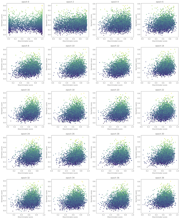
We are interested in the correlation between the semantic scores and discriminator scores of image captions as well as its evolution along the process of SCST GAN training. We provide scatter plots for the Joint-Embedding discriminator [4] across training in Figure 9. This GAN model was trained over 40 epochs with a discriminator pretrained on 15 epochs of data.
We compare semantic scores and discriminator scores over training epochs given the ground truth (GT) caption for each image in the COCO Test set (5K images). Each GT caption being fixed, we can observe the evolution of the semantic and discriminator score without any other effects. Figure 9 show the semantic score, discriminator score pairs for each image (one point per image) for the joint embedding discriminator. Since the GT captions are fixed, the semantic scores will be identical across epochs. From the first epoch, the joint embedding discriminator provides a wide range of scores with most scores close to the 0.0 and 1.0 min/max values. Quickly the points cluster into a ’sail’ like shape in the lower right corner, away from the min/max edges. The color assigned to each point is directly linked to the semantic scores assigned at the first epoch of training. You can therefore have a small visual cue of the movement of these points from epoch to epoch and witness the discriminator learning how to distinguish real and fake captions.
Appendix D Human Evaluation
In this section we present the details of our evaluation protocol for our captioning models on Amazon MTurk. All images are presented to 5 workers and aggregated in mean opinion score (MOS) or majority vote.
Turing Test.
In this setting we give human evaluators an image with a sentence either generated from our GAN captioning models or the ground truth. We ask them whether the sentence is human generated or machine generated. Exact instructions are: "Is this image caption written by a human? Yes/No. The caption could be written by a human or by a computer, more or less 50-50 chance."
Fine Grained Evaluation and Model Comparison.
In this experiment we give human evaluators an image and a set of 3 captions: Generated by CE trained model, SCST CIDEr trained model, and a GAN model. We ask them to rate each sentence on a scale of one to five. After rating, the worker chooses the caption he/she thinks is best at describing the image. In Section 4, we provide results for Mean Opinion Score and Majority vote based of this interface (see Figure 10) and Table 7.
| COCO Test | OOC | |||
| Semantic Score | MOS | Semantic Score | MOS | |
| EnsCE(CE) | 0.189 | 3.222 | 0.122 | 3.065 |
| EnsRL(CIDEr-RL) | 0.186 | 3.297 | 0.122 | 3.097 |
| Ens1(SCST, Co-att, ) | 0.195 | 3.398 | – | – |
| Ens2(SCST, Co-att, ) | 0.194 | 3.442 | 0.127 | 3.107 |
| Ens3(SCST, Joint-Emb, ) | 0.193 | 3.286 | – | – |
| Ens5(Gumbel Soft, Co-Att,) | 0.191 | 3.138 | – | – |
| Ens7(Gumbel ST, Co-Att, ) | 0.180 | 3.235 | – | – |
Appendix E Experimental Protocol SCST vs. Gumbel
In Figure 11, we show that all our Gumbel Methods trained effectively. We plot the Discriminator scores (averaged over minibatch) during training with the 3 reported Gumbel models. Generated sentences get roughly 0.5, random sentences around 0.1, real sentences around 0.75. Hence, the Discriminator can correctly distinguish real from random, and generated sentences. This indicates a healthy training of all Gumbel Methods.

Appendix F Examples of Generated Captions
In this section we present several examples of captions generated from our model. In particular, Figure 12 and Figure 13 show captions for randomly picked images (from COCO and OOC respectively) which provide a good description of the image content. We do the opposite in Figure 14 and Figure 15 where examples of bad captions are provided for COCO and OOC respectively.
(c)|c|c||c|c|c|c|
 &
&
GAN: a group of boats are docked in a harbor
CE: a group of boats sitting in the water
RL: a group of boats sitting in the water
GT: some boats parked in the water at a dock
GAN: a man holding a baseball bat at night
CE: a man is holding a bat in a dark
RL: a man holding a baseball bat at a ball
GT: a boy in yellow shirt swinging a baseball bat

GAN: a dog laying down on a person ’s lap
CE: a dog is sleeping on a couch with a person
RL: a dog laying on a couch with a person
GT: a dog that is laying next to another person
GAN: a bunch of umbrellas hanging from a wall in a store
CE: a bunch of umbrellas that are hanging from a wall
RL: a group of umbrellas hanging from a store
GT: a bunch of umbrellas that are behind a glass
(c)|c|c||c|c|c|c|
 &
&

GAN: a store front with a car parked in front of it
CE: a store with a sign on the side of it
RL: a building with a sign on the side of it
GT: a car has crashed into the store front of a chinese restaurant
GAN: a bed sitting in the middle of a forest
CE: a bed with a green blanket on it
RL: a bed in a forest with a table
GT: a bed lies on top of a clover field in a forest


GAN: a couch sitting in front of a house with a trash can
CE: a white couch sitting in front of a house
RL: a couch sitting in front of a house
GT: a white couch on top of a grass curb with a black table in the background
GAN: a large passenger jet taking off from a busy street
CE: a large passenger jet sitting on top of a runway
RL: a group of cars parked on the runway at an airplane
GT: an airplane descends very close to traffic stuck at a red light
(c)|c|c||c|c|c|c|
 &
&

GAN: a baseball player swinging a bat at a ball
CE: a baseball player is swinging a bat at a ball
RL: a baseball player swinging a bat at a ball
GT: a man that is standing in the dirt with a glove
GAN: a black and white photo of two men in suits
CE: a man and a woman standing next to each other
RL: a black and white photo of a man and a woman
GT: a man sitting next to a woman while wearing a suit


GAN: a woman sitting on a bench looking at her cell phone
CE: a woman sitting on a bench in a park
RL: a woman sitting on the ground next to a bench
GT: a woman is sitting with a suitcase on some train tracks
GAN: a bike that is in a room with a bike
CE: a bicycle with a bicycle and a bicycle in a room
RL: a room with a bed and a table in a room
GT: the hospital bed is metal and has wheels
(c)|c|c||c|c|c|c|
 &
&

GAN: a man standing on the side of the road with a skateboard
CE: a man standing on the side of a road with a cell phone
RL: a man standing on the side of a road with a cell phone
GT: a woman holds a drink can while holding the door to a refrigerator that is sitting on the asphalt of a street
GAN: two people walking on a beach with a dog
CE: a couple of people walking on a beach with a dog
RL: a group of people walking on a beach with a dog
GT: a lady is flying a chair as if its a kite while walking along the water edge

GAN: a couple of chairs and a blue beach chairs on a beach
CE: a couple of chairs sitting next to each other on a beach
RL: a group of chairs and a table in the beach
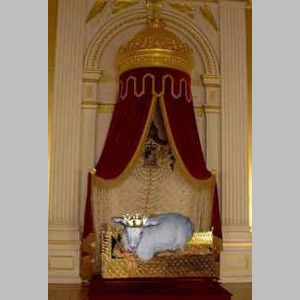
GT: a picture of a chair on an empty beach with a laptop on the arm
GAN: a painting of a vase in front of a fire hydrant
CE: a painting of a fire place in a room
RL: a bedroom with a bed and a clock on the wall
GT: a white goat wearing a gold crown sits on a gold bed