optimParallel: an R Package Providing Parallel Versions of the Gradient-Based Optimization Methods of optim()

Abstract

The R package optimParallel (Gerber, 2018) provides a parallel version of the gradient-based optimization methods of optim(). The main function of the package is optimParallel(), which has the same usage and output as optim(). Using optimParallel() can significantly reduce optimization times. We introduce the R package and illustrate its implementation, which takes advantage of the lexical scoping mechanism of R.

Introduction

Many statistical tools involve optimization algorithms, which aim to find the minima or maxima of a function $fn:\mathbb{R}^{p}\rightarrow\mathbb{R}$, where $p\in\mathbb{N}$ denotes the number of parameters. Depending on the specific application different optimization algorithms may be preferred; see the book by Nash (2014), the special issue of the Journal of Statistical Software (Varadhan, 2014), and the CRAN Task View Optimization for overviews of the optimization software available for R. Widely used algorithms are the gradient-based optimization methods denoted by "L-BFGS-B", "BFGS", and "CG", which are available through the general-purpose optimizer optim() of the R package stats; see the help page of optim() for more information. Those algorithms have proven to work well in numerous application. However, long optimization times of computationally intensive functions sometimes hinder their application; see Gerber et al. (2017) for an example of such a function from our research in spatial statistics. For this reason we present a parallel optim() version in this article and explore its potential to reduce optimization times.

The gradient-based optimization algorithms of optim() rely on the evaluation of the gradient of $fn()$ denoted by $gr:\mathbb{R}^{p}\rightarrow\mathbb{R}^{p}$. To illustrate the benefit of a parallel version of those algorithms we consider the optimization method "L-BFGS-B", which alternately evaluates $fn()$ and $gr()$. Let $T_{fn}$ and $T_{gr}$ denote the evaluation times of $fn()$ and $gr()$, respectively. In the case where $gr()$ is specified by the user, one iteration of the algorithm evaluates $fn()$ and $gr()$ sequentially at the same parameter value. Hence, the evaluation time of one iteration is $T_{fn}+T_{gr}$. In contrast, optimParallel() evaluates both functions in parallel using two processor cores, which reduces the evaluation time to little more than $\max\{T_{fn},T_{gr}\}$. In the case where no gradient is provided, optim() calculates a numeric central difference approximation of $gr()$. For $p=1$ that approximation is defined as

$$\widetilde{gr}(x)=(fn(x+\epsilon)-fn(x-\epsilon))\,/\,2\,\epsilon$$ (1)

and hence requires two evaluations of $fn()$. Similarly, calculating $\widetilde{gr}()$ requires $2p$ evaluations of $fn()$ if $fn()$ has $p$ parameters. In total, optim() sequentially evaluates $fn()$  $1+2p$ times per iteration, resulting in an elapsed time of $(1+2p)T_{fn}$. Given $1+2p$ available processor cores optimParallel() evaluates all calls of $fn()$ in parallel, which reduces the elapsed time to about $T_{fn}$ per iteration.

optimParallel() by example

The main function of the R package optimParallel is optimParallel(), which has the same usage and output as optim(), but evaluates $fn()$ and $gr()$ in parallel. For illustration, consider $1000$ samples from a normal distribution with mean $\mu=5$ and standard deviation $\sigma=2$. Then, we define the following negative log-likelihood and use optim() to estimate the parameters $\mu$ and $\sigma$.

> x <- rnorm(n = 1000, mean = 5, sd = 2)> negll <- function(par, x) -sum(dnorm(x = x, mean = par[1], sd = par[2], log = TRUE))> o1 <- optim(par = c(1, 1), fn = negll, x = x, method = "L-BFGS-B",+             lower = c(-Inf, 0.0001))> o1$par[1] 5.017583 1.991459

Using optimParallel(), we can do the same in parallel. The functions makeCluster(), detectCores(), and setDefaultCluster(), from the R package parallel are used to set up a default cluster for parallel execution.

> install.packages("optimParallel")> library("optimParallel")> cl <- makeCluster(detectCores()); setDefaultCluster(cl = cl)> o2 <- optimParallel(par = c(1, 1), fn = negll, x = x, method = "L-BFGS-B",+                     lower = c(-Inf, 0.0001))> identical(o1, o2)[1] TRUE

In addition to the arguments of optim(), optimParallel() has the argument parallel, which takes a list of arguments. For example, we can set loginfo = TRUE to store the evaluated parameters and the corresponding gradients.

> o3 <- optimParallel(par = c(1, 1), fn = negll, x = x, method = "L-BFGS-B",+                     lower = c(-Inf, 0.0001), parallel=list(loginfo = TRUE))> print(o3$loginfo[1:3, ], digits = 3)     iter par1 par2    fn   gr1    gr2[1,]    1 1.00 1.00 10640 -3928 -18442[2,]    2 1.21 1.98  3882  -951  -1801[3,]    3 1.27 2.09  3655  -842  -1441This can be used to visualize the optimization path as shown in Figure 1.

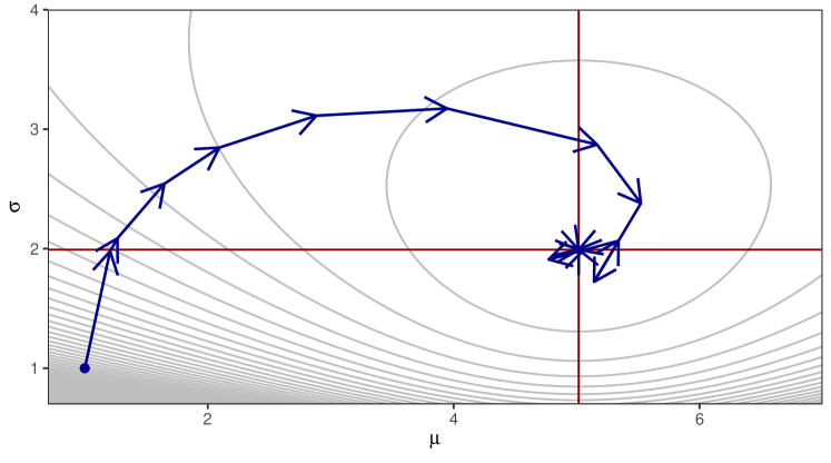
Figure 1: Visualization of the optimization path based on the log information obtained with optimParallel(..., parallel = list(loginfo = TRUE)). The red lines mark the estimates $\hat{\mu}$ and $\hat{\sigma}$.

Another option is forward, which can be set to TRUE to enable the numeric forward difference approximation defined as $\widetilde{gr}(x)=(fn(x+\epsilon)-fn(x))/\epsilon\,$ for $p=1$ and $x$ sufficiently away from the boundaries. Using that approximation, the return value of $fn(x)$ can be reused, and hence, the number of evaluations of $fn()$ is reduced to $1+p$ per iteration. This is helpful if the number of available cores is less that $1+2p$.

Implementation

optimParallel() is a wrapper to optim() and enables the parallel evaluation of all function calls involved in one iteration of the gradient-based optimization methods. It is implemented in R and interfaces compiled C code only through optim(). The reuse of the stable and well-tested C code of optim() has the advantage that optimParallel() leads to the exact same results as optim(). To ensure that optimParallel() and optim() indeed return the same results optimParallel contains systematic unit tests implemented with the R package testthat (Wickham, 2017, 2011).

The basic idea of the implementation is that calling fn() (or gr()) triggers the evaluation of both fn() and gr(). Their return values are stored in a local environment. The next time fn() (or gr()) is called with the same parameters the results are read from the local environment without evaluating fn() and gr() again. The following R code illustrates how optimParallel() takes advantage of the lexical scoping mechanism of R to store the return values of fn() and gr().

> demo_generator <- function(fn, gr) {+     par_last <- value <- grad <- NA+     eval <- function(par) {+         if(!identical(par, par_last)) {+             message("--> evaluate fn() and gr()")+             par_last <<- par+             value <<- fn(par)+             grad <<- gr(par)+         } else+             message("--> read stored value")+     }+     f <- function(par) {+         eval(par = par)+         value+     }+     g <- function(par) {+         eval(par = par)+         grad+     }+     list(f = f, g = g)+ }> demo <- demo_generator(fn = sum, gr = prod)Calling demo$f() triggers the evaluation of both fn() and gr().

> demo$f(1:5)--> evaluate fn() and gr()[1] 15The subsequent call of demo$g() with the same parameters returns the stored value grad without evaluating gr() again.

> demo$g(1:5)--> read stored value[1] 120A similar construct allows optimParallel() to evaluate $fn()$ and $gr()$ at the same occasion. It is then straightforward to parallelize the evaluations using the R package parallel.

Benchmark

To illustrate the speed gains that can be achieved with optimParallel() we measure the elapsed times per iteration when optimizing the following test function and compare them to those of optim().

> fn <- function(par, sleep) {+     Sys.sleep(sleep)+     sum(par^2)+ }> gr <- function(par, sleep) {+     Sys.sleep(sleep)+     2*par+ }In both functions the argument par can be a numeric vector with one or more elements and the argument sleep controls the evaluation time of the functions. We measure the elapsed time per iteration for method = "L-BFGS-B" using all combinations of $p=1$, $2$, $3$, sleep = $0$, $0.05$, $0.2$, $0.4$, $0.6$, $0.8$, and $1$ seconds with and without analytic gradient gr(). All measurements are taken on a computer with $12$ Intel Xeon E5-2640 @ 2.50GHz processors. However, because of the experimental design maximum $7$ processors are used in parallel. We repeat each measurement $5$ times using the R package microbenchmark (Mersmann et al., 2018). The complete R script of the benchmark experiment is contained in optimParallel.

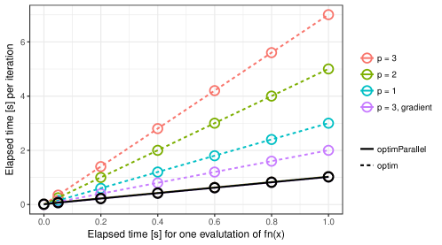
Figure 2: Benchmark experiment comparing the "L-BFGS-B" method from optimParallel() and optim(). Plotted are the elapsed times per iteration ($y$-axis) and the evaluation time of $fn()$ ($x$-axis) for $p=1,\,2,$ and $3$ using an approximate gradient and $p=3$ using an analytic gradient. The elapsed times of optimParallel() (solid line) are independent of $p$ and the specification of an analytic gradient.

The results of the benchmark experiment are summarized in Figure 2. They show that for optimParallel() the elapsed time per iteration is only marginally larger than $T_{fn}$ (black dots in Figure 2). Conversely, the elapsed time for optim() is $T_{fn}+T_{gr}$ if a gradient function is specified (violet dots) and $(1+2p)T_{fn}$ if no gradient function is specified. Moreover, optimParallel() adds a small overhead, and hence, it is only faster than optim() if $T_{fn}$ is larger than $0.05$ seconds.

Summary

The R package optimParallel provides parallel versions of the gradient-based optimization methods "L-BFGS-B", "BFGS", and "CG" of optim(). After a brief theoretical illustration of the possible speed improvement based on parallel processing, we illustrate optimParallel() by examples. The examples demonstrate that one can replace optim() by optimParallel() to execute the optimization in parallel and illustrate additional features like capturing log information and the forward gradient approximation. Moreover, we briefly sketch the basic idea of the implementation, which is based on the lexical scoping mechanism of R. Finally, a benchmark experiment shows that using optimParallel() reduces the elapsed time to optimize computationally demanding functions significantly. For functions with evaluation times of more than $0.05$ seconds we measured speed gains of about factor $2$ in the case where an analytic gradient was specified and about factor $1+2p$ otherwise ($p$ is the number of parameters).

Dr. Florian Gerber
Department of Mathematics, University of Zurich, Switzerland
florian.gerber@math.uzh.ch, https://orcid.org/0000-0001-8545-5263

Prof. Dr. Reinhard Furrer
Department of Mathematics & Department of Computational Science, University of Zurich, Switzerland
reinhard.furrer@math.uzh.ch, https://orcid.org/0000-0002-6319-2332

References

- Gerber (2018) F. Gerber. optimParallel: Parallel Versions of the Gradient-Based optim() Methods, 2018. URL https://git.math.uzh.ch/florian.gerber/optimParallel. R package version 0.7.
- Gerber et al. (2017) F. Gerber, K. Mösinger, and R. Furrer. Extending R packages to support 64-bit compiled code: An illustration with spam64 and GIMMS NDVI data. Comput. Geosci., 104:109–119, 2017. URL https://doi.org/10.1016/j.cageo.2016.11.015.
- Mersmann et al. (2018) O. Mersmann, C. Beleites, R. Hurling, A. Friedman, and J. M. Ulrich. microbenchmark: Accurate timing functions, 2018. URL https://CRAN.R-project.org/package=microbenchmark. R package version 1.4-4.
- Nash (2014) J. C. Nash. Nonlinear Parameter Optimization Using R Tools. Wiley & Sons, Ltd, 2014. ISBN 9781118883969. URL https://doi.org/10.1002/9781118884003.
- Varadhan (2014) R. Varadhan. Special volume: Numerical optimization in R: Beyond optim. Journal of Statistical Software, 6, 2014. ISSN 1548-7660. URL https://www.jstatsoft.org/issue/view/v060.
- Wickham (2011) H. Wickham. testthat: Get started with testing. R J., 3:5–10, 2011. URL http://journal.R-project.org/archive/2011-1/RJournal_2011-1_Wickham.pdf.
- Wickham (2017) H. Wickham. testthat: Unit Testing for R, 2017. URL https://CRAN.R-project.org/package=testthat. R package version 2.0.0.