Supervised by:		Submitted by:
Prof. Arvind &		Harpreet Singh
Dr. Kavita Dorai

Indian Institute of Science Education & Research Mohali
Mohali - 140 306
India
(September 2017)

Declaration

The work presented in this thesis has been carried out by me under the guidance of Prof. Arvind and Dr. Kavita Dorai at the Indian Institute of Science Education and Research Mohali.

This work has not been submitted in part or in full for a degree, diploma or a fellowship to any other University or Institute. Whenever contributions of others are involved, every effort has been made to indicate this clearly, with due acknowledgement of collaborative research and discussions. This thesis is a bonafide record of original work done by me and all sources listed within have been detailed in the bibliography.

Harpreet Singh

Place :
Date :

In our capacity as supervisors of the candidate’s PhD thesis work, we certify that the above statements by the candidate are true to the best of our knowledge.

Dr. Kavita Dorai                                                 Dr. Arvind
Associate Professor                                               Professor
Department of Physical Sciences                            Department of Physical Sciences
IISER Mohali                                                       IISER Mohali

Place :                                                                  Place :
Date :                                                                  Date :

Acknowledgements

I owe a huge gratitude to my PhD advisors Dr. Kavita Dorai and Prof. Arvind for teaching the basics of NMR technique and Quantum Information Processing. I must admit that without their help and support this thesis would not have been possible.

I would like to thank my doctoral committee member Dr. Abhishek Chaudhuri for his useful advices. I am grateful to Prof. N Sathyamurthy, the Director of IISER Mohali for providing all kind of help needed for my research work. I am thankful to the faculty of the Department of Physical Sciences of IISER Mohali for providing their excellent guidance during my course work.

I am grateful to the NMR and QCQI group IISER Mohali for discussions and presentations. I would like to acknowledge the support from my group members: Satnam Singh, Navdeep Gogna, Amandeep Singh, Rakesh Sharma, Jyotsana Ojha, Jaskaran Singh, Chandan Sharma, Akash Sherawat, Akshay Gaikwad, Rajendera Singh Bhati, Akansha Gautam, Amit Devra, Gaurav Saxena, Dileep Singh and Aditya Mishra, Amrita Kumari and Matsyendra Nath Shukla. I am specially grateful to Ritabrata Sengupta, Debmayla Das and Shruti Dogra for the useful discussions and providing all kind of support in my research work.

I owe my special thanks to Dr. Paramdip Singh Chandi for helping us troubleshooting the errors in the lab machines. At the same time, I am thankful to Dr B. S. Joshi (Application, Bruker India) for his technical support and guidance.

I have benefited a lot from discussions with Gopal Verma, Anshul Choudhary, Vivek Kohar, Kanika Pasrija and Satyam Ravi during course work. I am grateful to my hostel friends Preetinder Singh, Bhupesh Garg, Nayyar Aslam, George Thomas, Navnoor Kaur Saran and Junaid Khan because of whom I enjoyed my hostel life.

I would like to thank my sisters Hardeep Kaur, Harveen Kaur and cousin Jasjeet Singh for their immense support and encouragement. I would also like to thank my brother-in-law Amandeep Singh for his continuous encouragement and guidance. I bow my head to my parents and grandparents for their generous invaluable blessings.

I am obliged to NMR research facility of IISER Mohali for providing me the platform for carrying out my research. During this thesis, various experiments were performed on 600 MHz Bruker NMR spectrometers using QXI, TXI and BBI probeheads.

I would like to acknowledge the financial support from Council of Scientific & Industrial Research (CSIR) during my PhD. I would like to thank IISER Mohali for providing fund for participation in EUROMAR 2015, held in Prague Czech Republic.

Finally, thanks to my wonderful niece Divjot Kaur for keeping the enthusiasm and positivity alive, which was required for my PhD completion.

Harpreet Singh

Abstract

This thesis deals with the generation, estimation and preservation of novel quantum states of two and three qubits on an NMR quantum information processor. Using the maximum likelihood ansatz, a method has been developed for state estimation such that the reconstructed density matrix does not have negative eigenvalues and the errors are within the space of valid density operators. Due to interactions with the environment, unwanted changes occur in the system, leading to decoherence. Controlling decoherence is one of the biggest challenges to be overcome to build quantum computers. To decouple the quantum system from its environment, several experimental strategies have been used. These strategies are based on our knowledge of system-environment interaction and states that need to be preserved. Considering the first case, where the system state is known but there is no knowledge about its interaction with the environment. To tackle decoherence in this case, the super-Zeno scheme is used and its efficacy to preserve quantum states is demonstrated. The next situation considered is that where only the subspace to which the system state belongs is known. To address such a situation, the nested Uhrig dynamical decoupling scheme has been used. The later part of the thesis deals with situations where the state of the system as well as its interaction with the environment is known. In such situations, since the noise model is known, decoupling strategies can be explicitly designed to cancel this noise. Using these decoupling strategies, the lifetime of time-invariant discord of two-qubit Bell-diagonal states has been experimentally extended. The decay of three-qubit entangled states namely the GHZ state, the W state and the $\rm W\bar{W}$ state are studied, and the noise model is constructed for the spin system. The experimentally observed and theoretical expected entanglement decay rates of these states are compared. Then, the dynamical decoupling scheme is applied to these states and remarkable protection is observed in the case of the GHZ state and the $W\bar{W}$ state.

The contents of the thesis have been divided into seven chapters whose brief account is sketched below:

Chapter 1

This chapter provides an introduction to the field of NMR quantum computation and quantum information as well as the motivation for the present thesis. In addition to the basics of NMR and quantum computation, recent developments in the field of quantum computation and quantum information are discussed.

Chapter 2

This chapter describes the utility of the maximum likelihood (ML) estimation scheme to estimate quantum states on an NMR quantum information processor. Various separable and entangled states of two and three qubits are experimentally prepared, and the density matrices are reconstructed using both the ML estimation scheme as well as standard quantum state tomography (QST). Further, an entanglement parameter is defined to quantify multiqubit entanglement and entanglement is estimated using both the QST and the ML estimation schemes.

Chapter 3

This chapter experimentally demonstrates the freezing of evolution of quantum states in one- and two-dimensional subspaces of two qubits on an NMR quantum information processor. The state evolution is frozen and leakage of the state from its subspace to an orthogonal subspace is successfully prevented using super-Zeno sequences. The super-Zeno scheme comprises a set of radio frequency (rf) pulses, punctuated by pre-selected time intervals. The efficacy of the scheme is demonstrated by preserving different types of states, including separable and maximally entangled states in one- and two-dimensional subspaces of a two-qubit system. The changes in the experimental density matrices are tracked by carrying out full state tomography at several time points. For the one-dimensional case, the fidelity measure is used and for the two-dimensional case, the leakage (fraction) into the orthogonal subspace is used as a qualitative indicator to estimate the resemblance of the density matrix at a later time to the initially prepared density matrix. For the case of entangled states, an entanglement parameter is computed additionally to indicate the presence of entanglement in the state at different times. The experiments demonstrate that the super-Zeno scheme is able to successfully confine state evolution to the one- or two-dimensional subspace being protected.

Chapter 4

In this chapter, the efficacy of a three-layer nested Uhrig dynamical decoupling (NUDD) sequence to preserve arbitrary quantum states in a two-dimensional subspace of the four-dimensional two-qubit Hilbert space is experimentally demonstrated on an NMR quantum information processor. The effect of the state preservation is studied first on four known states, including two product states and two maximally entangled Bell states. Next, to evaluate the preservation capacity of the NUDD scheme, it is applied to eight randomly generated states in the subspace. Although, the preservation of different states varies, the scheme on the average performs very well. The complete tomographs of the states at different time points are used to compute fidelity. The state fidelities using NUDD protection are compared with those obtained without using any protection.

Chapter 5

The discovery of the intriguing phenomenon that certain kinds of quantum correlations remain impervious to noise up to a specific point in time and then suddenly decay, has generated immense recent interest. In this chapter, dynamical decoupling sequences are exploited to prolong the persistence of time-invariant quantum discord in a system of two NMR qubits decohering in independent dephasing environments. Noise channels affecting the considered spin system of the molecule are characterized and each spin of the spin system is mainly affected by the independent phase damping channel. Bell-diagonal quantum states are experimentally prepared on a two-qubit NMR processor, and robust dynamical decoupling schemes are applied for state preservation. It is demonstrated that these schemes are able to successfully extend the lifetime of time-invariant quantum discord.

Chapter 6

This chapter demonstrates the experimental protection of different classes of tripartite entangled states, namely the maximally entangled GHZ and W states and the ${\rm W\bar{W}}$ state, using dynamical decoupling. The states are created on a three-qubit NMR quantum information processor and allowed to evolve in the naturally noisy NMR environment. The tripartite entanglement is monitored at each time instant during state evolution, using negativity as an entanglement measure. It is observed that the W state is the most robust while the GHZ-type states are the most fragile against the natural decoherence present in the NMR system. The ${\rm W\bar{W}}$ state which is in the GHZ-class, yet stores entanglement in a manner akin to the W state, surprisingly turns out to be more robust than the GHZ state. The experimental data are best modeled by considering the main noise channel to be an uncorrelated phase damping channel acting independently on each qubit, along with a generalized amplitude damping channel. Using dynamical decoupling, a significant protection of entanglement for GHZ state is achieved. There is a marginal improvement in the state fidelity for the W state (which is already robust against natural system decoherence), while the ${\rm W\bar{W}}$ state shows a significant improvement in fidelity and protection against decoherence.

Chapter 7

This chapter provides some general remarks on the problems covered in the thesis. Possible future applications of the state protection techniques used in this thesis and the new avenues of research they open up are described. The overall contribution of this thesis in the context of the study of decoherence and state preservation techniques in quantum information processing, is summarized.

List of Publications

1. Harpreet Singh, Arvind and Kavita Dorai. Experimental protection against evolution of states in a subspace via a super-Zeno scheme on an NMR quantum information processor. Phys. Rev. A, 90, 052329 (2014).

2. Harpreet Singh, Arvind and Kavita Dorai. Constructing valid density matrices on an NMR quantum information processor via maximum likelihood estimation. Phys. Lett. A, 380 3051 (2016).

3. Harpreet Singh, Arvind and Kavita Dorai. Experimental protection of arbitrary states in a two-qubit subspace by nested Uhrig dynamical decoupling. Phys. Rev. A, 95, 052337 (2017).

4. Harpreet Singh, Arvind and Kavita Dorai. Experimentally freezing quantum discord in a dephasing environment using dynamical decoupling. EPL, 118, 50001 (2017).

5. Rakesh Sharma, Navdeep Gogna,Harpreet Singh, Kavita Dorai. Fast profiling of metabolite mixtures using chemometric analysis of a speeded-up 2D heteronuclear correlation NMR experiment. RSC Adv., 7, 29860 (2017).

6. Harpreet Singh, Arvind and Kavita Dorai. Evolution of tripartite entangled states in a decohering environment and their experimental protection using dynamical decoupling. PhysRevA, 97, 022302 (2018).

7. Amit Devra, Prithviraj Prabhu,Harpreet Singh and Kavita Dorai. Efficient experimental design of high-fidelity three-qubit quantum gates via genetic programming.Quantum Inf Process, 17, 67 (2018).

8. Harpreet Singh, Arvind and Kavita Dorai. Multiple-quantum relaxation in three-spin homonuclear and heteronuclear systems: An integrated Redfield and Lindblad master-equation approach. (Manuscript in preparation 2017).

Contents

1. Abstract
2. 1 Introduction
   1. 1.1 Quantum computing and quantum information processing
      1. 1.1.1 Quantum bit
      2. 1.1.2 $N$-qubit quantum register
      3. 1.1.3 Density matrix representation
      4. 1.1.4 Quantum gates
      5. 1.1.5 Quantum measurement
   2. 1.2 Nuclear Magnetic Resonance
   3. 1.3 NMR quantum computing
      1. 1.3.1 NMR qubits
      2. 1.3.2 Initialization
      3. 1.3.3 Quantum gate implementation in NMR
      4. 1.3.4 Numerical techniques for quantum gate optimization
      5. 1.3.5 Measurement in NMR
   4. 1.4 Evolution of quantum systems
      1. 1.4.1 Closed quantum systems
      2. 1.4.2 Open systems
      3. 1.4.3 Quantum noise channels
         1. 1.4.3.1 Generalized amplitude damping channel
         2. 1.4.3.2 Phase damping channel
         3. 1.4.3.3 Depolarizing channel
      4. 1.4.4 Nuclear spin relaxation
      5. 1.4.5 Longitudinal relaxation
      6. 1.4.6 Transverse relaxation
      7. 1.4.7 Bloch-Wangness-Redfield relaxation theory
   5. 1.5 Decoherence suppression
      1. 1.5.1 Hahn echo
      2. 1.5.2 CPMG DD sequence
      3. 1.5.3 Uhrig DD sequence
      4. 1.5.4 Super-Zeno Scheme
      5. 1.5.5 Nested Uhrig dynamical decoupling
   6. 1.6 Organization of the thesis
3. 2 State tomography on an NMR quantum information processor via maximum likelihood estimation
   1. 2.1 Introduction
      1. 2.1.1 NMR quantum state tomography
      2. 2.1.2 Maximum likelihood estimation
   2. 2.2 Comparison of quantum state estimation via ML estimation and standard QST schemes
      1. 2.2.0.1 Fidelity measure and state estimation
      2. 2.2.1 Comparison of separable states estimation
      3. 2.2.2 Comparison of entangled states estimation
   3. 2.3 Conclusions
4. 3 Experimental protection of quantum states via a super-Zeno scheme
   1. 3.1 Introduction
   2. 3.2 The super-Zeno scheme
   3. 3.3 Experimental implementations of super-Zeno scheme
      1. 3.3.1 NMR system details
      2. 3.3.2 Super-Zeno scheme for state preservation
         1. 3.3.2.1 Preservation of product states:
         2. 3.3.2.2 Preservation of entangled states
         3. 3.3.2.3 Estimation of state fidelity
      3. 3.3.3 Super-Zeno for subspace preservation
         1. 3.3.3.1 Preservation of product states in the subspace
         2. 3.3.3.2 Preservation of an entangled state in the subspace
         3. 3.3.3.3 Estimating leakage outside subspace
      4. 3.3.4 Preservation of entanglement
   4. 3.4 Conclusions
5. 4 Experimental protection of unknown states using nested Uhrig dynamical decoupling sequences
   1. 4.1 Introduction
   2. 4.2 The NUDD scheme
   3. 4.3 Experimental protection of two qubits using NUDD
      1. 4.3.1 Experimental implementation of the NUDD scheme
      2. 4.3.2 NUDD protection of known states in the subspace
      3. 4.3.3 NUDD protection of unknown states in the subspace
   4. 4.4 Conclusions
6. 5 Experimentally preserving time-invariant discord using dynamical decoupling
   1. 5.1 Introduction
   2. 5.2 Measure for correlations of two qubits
   3. 5.3 Characterization of noise channels
      1. 5.3.1 Bell-diagonal states under a dephasing channel
   4. 5.4 Time invariant quantum correlations
   5. 5.5 Experimental realization of time-invariant discord
      1. 5.5.1 NMR System
      2. 5.5.2 Observing time-invariant discord
   6. 5.6 Protection of time-invariant discord using dynamical decoupling schemes
      1. 5.6.1 Conclusions
7. 6 Dynamics of tripartite entanglement under decoherence and protection using dynamical decoupling
   1. 6.1 Introduction
   2. 6.2 Dynamics of tripartite entanglement
      1. 6.2.1 Tripartite entanglement under different noise channels
      2. 6.2.2 NMR system
      3. 6.2.3 Construction of tripartite entangled states
      4. 6.2.4 Decay of tripartite entanglement
   3. 6.3 Protecting three-qubit entanglement via dynamical decoupling
   4. 6.4 Conclusions
8. 7 Summary and future outlook

List of Figures

1. 1.1 Bloch sphere representation of a qubit.
2. 1.2 (a) NMR tube with sample oriented in a strong static magnetic field $B_{0}$ along the $z$-axis and time-dependent magnetic field $B_{1}(t)$ along the $x$-axis. (b) The number of spins precessing around the direction parallel to the field are more than the number antiparallel to the field direction, which creates a bulk magnetization $M_{0}$.
3. 1.3 Populations of energy levels of a two-qubit system of a (a) thermal equilibrium state and (b) a pseudopure state.
4. 1.4 Plot of rf pulse amplitude and phase with time, optimized with GRAPE for CSWAP gate.
5. 1.5 Rotation of Bulk magnetization using resonance. $B_{1}(t)$ applied in -x-direction for duration such that total rotation is $90^{\circ}$
6. 1.6 (a) Representation of a closed system; the circle around the system depicts no interaction between the system and environment. (b) Representation of an open system; the dashed circle around the system shows that the system and environment are interacting.
7. 1.7 Model of closed quantum systems.
8. 1.8 Model of open quantum system consisting of two parts: the principal system and its environment.
9. 1.9 Evolution of the bulk magnetization under Hahn echo sequence. (a) Initially thermal equilibrium bulk magnetization in $z$ direction is represented by an arrow. (b) Bulk magnetization rotated to $-y$ axis using $90^{\circ}$ pulse, (c) A delay of time $t$ is given and arrows represent different spins, (d) $180^{\circ}$ is applied to spins due to which a spin precessing fast will fall behind a spin precessing slowly, and (e) after time $t$, all the spins are in the same direction.
10. 1.10 Pulse sequence of CPMG DD sequence for a cycle of duration $T$ and in one cycle eight pulses are applied; filled bars represent $\pi$ rotation pulses and $\tau$ is the duration between two consecutive $\pi$ pulses.
11. 1.11 Pulse sequence for UDD sequence for a cycle time of $T$ and the number of $\pi$ pulses in one cycle of sequence is eight. Filled bars represent $\pi$ rotation pulses.
12. 2.1 Real (left) and imaginary (right) parts of the experimental tomographs of the (a) $|00\rangle$ state, with a computed fidelity of 0.9937 using standard QST and a computed fidelity of 0.9992 using ML method for state estimation. (b) $\frac{1}{\sqrt{2}}(|00\rangle+|01\rangle)$ state, with a computed fidelity of 0.9928 using standard QST and a computed fidelity of 0.9991 using ML method for state estimation. The rows and columns are labeled in the computational basis ordered from $|00\rangle$ to $|11\rangle$.
13. 2.2 Real (left) and imaginary (right) parts of the experimental tomographs of the entangled state $\frac{1}{\sqrt{2}}(|01\rangle+|10\rangle)$ reconstructed (a) using standard QST and (b) using ML estimation. The fidelities computed using standard QST and using ML method for state estimation are 0.9933 and 0.9999 respectively. The rows and columns are labeled in the computational basis ordered from $|00\rangle$ to $|11\rangle$.
14. 2.3 Real (left) and imaginary (right) parts of the experimental tomographs of the three-qubit maximally entangled state $|W\rangle=\frac{1}{\sqrt{3}}(i|001\rangle+|010\rangle+|100\rangle)$, reconstructed (a) using standard QST with a computed fidelity of 0.9833 and (b) using ML estimation with a computed fidelity of 0.9968. The rows and columns are labeled in the computational basis ordered from $|000\rangle$ to $|111\rangle$.
15. 2.4 Real (left) and imaginary (right) parts of the experimental tomographs of the (a) $\frac{1}{\sqrt{2}}(|00\rangle+|11\rangle)$ state. Tomographs (b)-(e) depict the state at $T=0.04,0.08,0.12,0.16s$, with the tomographs on the left and the right representing the state estimated using standard QST and using ML estimation, respectively. The rows and columns are labeled in the computational basis ordered from $|00\rangle$ to $|11\rangle$.
16. 2.5 Plot of the entanglement parameter $\eta$ with time, using standard QST and ML protocols for state reconstruction, computed for the $\frac{1}{\sqrt{2}}(|00\rangle+|11\rangle)$ state.
17. 3.1 (a) Molecular structure of cytosine with the two qubits labeled as $H^{1}$ and $H^{2}$ and tabulated system parameters with chemical shifts $\nu_{i}$ and scalar coupling $J_{12}$ (in Hz) and relaxation times $T_{1}$ and $T_{2}$ (in seconds) (b) NMR spectrum obtained after a $\pi/2$ readout pulse on the thermal equilibrium state. The resonance lines of each qubit are labeled by the corresponding logical states of the other qubit and (c) NMR spectrum of the pseudopure $|00\rangle$ state.
18. 3.2 (a) Quantum circuit for preservation of the state $|11\rangle$ using the super-Zeno scheme. $\Delta_{i}=x_{i}t,(i=1...5)$ denote time intervals punctuating the unitary operation blocks. Each unitary operation block contains a controlled-phase gate ($Z$), with the first (top) qubit as the control and the second (bottom) qubit as the target. The entire scheme is repeated $N$ times before measurement (for our experiments $N=30$). (b) Block-wise depiction of the corresponding NMR pulse sequence. A $z$-gradient is applied just before the super-Zeno pulses, to clean up undesired residual magnetization. The unfilled and black rectangles represent hard $180^{0}$ and $90^{0}$ pulses respectively, while the unfilled and gray-shaded conical shapes represent $180^{0}$ and $90^{0}$ pulses (numerically optimized using GRAPE) respectively; $\tau_{12}$ is the evolution period under the $J_{12}$ coupling. Pulses are labeled with their respective phases and unless explicitly labeled, the phase of the pulses on the second (bottom) qubit are the same as those on the first (top) qubit.
19. 3.3 Real (left) and imaginary (right) parts of the experimental tomographs of the (a) $|11\rangle$ state, with a computed fidelity of 0.99. (b)-(e) depict the state at $T=0.61,3.03,5.46,7.28$ s, with the tomographs on the left and the right representing the state without and after applying the super-Zeno preserving scheme, respectively. The rows and columns are labeled in the computational basis ordered from $|00\rangle$ to $|11\rangle$.
20. 3.4 (a) Quantum circuit for preservation of the singlet state using the super-Zeno scheme. $\Delta_{i},(i=1...5)$ denote time intervals punctuating the unitary operation blocks. The entire scheme is repeated $N$ times before measurement (for our experiments $N=10$). (b) NMR pulse sequence corresponding to one unitary block of the circuit in (a). A $z$-gradient is applied just before the super-Zeno pulses, to clean up undesired residual magnetization. The unfilled rectangles represent hard $180^{0}$ pulses, the black filled rectangles representing hard $90^{0}$ pulses, while the shaded shapes represent numerically optimized (using GRAPE) pulses and the gray-shaded shapes representing $90^{0}$ pulses respectively; $\tau_{12}$ is the evolution period under the $J_{12}$ coupling. Pulses are labeled with their respective phases and unless explicitly labeled, the phase of the pulses on the second (bottom) qubit are the same as those on the first (top) qubit.
21. 3.5 Real (left) and imaginary (right) parts of the experimental tomographs of the (a) $\frac{1}{\sqrt{2}}(|01\rangle-|10\rangle)$ (singlet) state, with a computed fidelity of 0.99. (b)-(e) depict the state at $T=0.85,2.54,4.24,5.93$ s, with the tomographs on the left and the right representing the state without and after applying the super-Zeno preserving scheme, respectively. The rows and columns are labeled in the computational basis ordered from $|00\rangle$ to $|11\rangle$.
22. 3.6 Plot of fidelity versus time of (a) the $|11\rangle$ state and (b) the $\frac{1}{\sqrt{2}}(|01\rangle-|10\rangle)$ (singlet) state, without any preserving scheme and after the super-Zeno preserving sequence. The fidelity of the state with the super-Zeno preservation remains close to 1.
23. 3.7 Plot of signal intensity versus time of the $|11\rangle$ state and the $\frac{1}{\sqrt{2}}(|01\rangle-|10\rangle)$ (singlet) state, after the super-Zeno preserving sequence.
24. 3.8 (a) Quantum circuit for preservation of the $\{01,10\}$ subspace using the super-Zeno scheme. $\Delta_{i},(i=1...5)$ denote time intervals punctuating the unitary operation blocks. The entire scheme is repeated $N$ times before measurement (for our experiments $N=30$). (b) NMR pulse sequence corresponding to the circuit in (a). A $z$-gradient is applied just before the super-Zeno pulses, to clean up undesired residual magnetization. The unfilled rectangles represent hard $180^{0}$ pulses; $\tau_{12}$ is the evolution period under the $J_{12}$ coupling. Pulses are labeled with their respective phases.
25. 3.9 Real (left) and imaginary (right) parts of the experimental tomographs of the (a) $|10\rangle$ state in the two-dimensional subspace $\{01,10\}$, with a computed fidelity of 0.98. (b)-(e) depict the state at $T=1.15,3.45,5.75,7.48$ s, with the tomographs on the left and the right representing the state without and after applying the super-Zeno preserving scheme, respectively. The rows and columns are labeled in the computational basis ordered from $|00\rangle$ to $|11\rangle$.
26. 3.10 Real (left) and imaginary (right) parts of the experimental tomographs of the (a) $|01\rangle$ state in the two-dimensional subspace $\{01,10\}$, with a computed fidelity of 0.99. (b)-(e) depict the state at $T=1.15,3.45,5.75,7.48$ s, with the tomographs on the left and the right representing the state without and after applying the super-Zeno preserving scheme, respectively. The rows and columns are labeled in the computational basis ordered from $|00\rangle$ to $|11\rangle$.
27. 3.11 Real (left) and imaginary (right) parts of the experimental tomographs of the (a) $\frac{1}{\sqrt{2}}(|01\rangle-|10\rangle)$ (singlet) state in the two-dimensional subspace $\{01,10\}$, with a computed fidelity of 0.98. (b)-(e) depict the state at $T=1.15,3.46,5.77,7.50$ s, with the tomographs on the left and the right representing the state without and after applying the super-Zeno preserving scheme, respectively. The rows and columns are labeled in the computational basis ordered from $|00\rangle$ to $|11\rangle$.
28. 3.12 Plot of leakage fraction from the $\{|01\rangle,|10\rangle\}$ subspace to its orthogonal subspace $\{|00\rangle,|11\rangle\}$ of (a) the $|10\rangle$ state and (b) the $\frac{1}{\sqrt{2}}(|01\rangle-|10\rangle)$ (singlet) state, without any preservation and after applying the super-Zeno sequence. The leakage to the orthogonal subspace is minimal (remains close to zero) after applying the super-Zeno scheme.
29. 3.13 Plot of entanglement parameter $\eta$ with time, with and without applying the super-Zeno sequence, computed for (a) the $\frac{1}{\sqrt{2}}(|01\rangle-|10\rangle)$ (singlet) state, and (b) the same singlet state when embedded in the subspace $\{|01\rangle,|10\rangle\}$ being preserved.
30. 4.1 (a) Circuit diagram for the three-layer NUDD sequence. The innermost UDD layer consists of $X_{0}$ control pulses, the middle layer comprises $X_{1}$ control pulses and the outermost layer consists of $X_{\phi}$ pulses. The entire NUDD sequence is repeated $M$ times; $\Delta_{i}$ are time intervals. (b) NMR pulse sequence to implement the control pulses for $X_{0}$ and $X_{1}$ UDD sequences. The values of the rf pulse phases $\phi_{1}$ and $\phi_{2}$ are set to $x$ and $y$ for the $X_{0}$ and to $-x$ and $-y$ for the $X_{1}$ UDD sequence, respectively. (c) NMR pulse sequence to implement the control pulses for the $X_{\phi}$ UDD sequence. The filled rectangles denote $\pi/2$ pulses while the unfilled rectangles denote $\pi$ pulses, respectively. The time period $\tau_{12}$ is set to the value $(2J_{12})^{-1}$, where $J_{12}$ denotes the strength of the scalar coupling between the two qubits.
31. 4.2 (a) Structure of isotopically enriched chloroform-¹³C molecule, with the ¹H spin labeling the first qubit and the ¹³C spin labeling the second qubit. The system parameters are tabulated alongside with chemical shifts $\nu_{i}$ and scalar coupling $J_{12}$ (in Hz) and NMR spin-lattice and spin-spin relaxation times $T_{1}$ and $T_{2}$ (in seconds). (b) NMR spectrum obtained after a $\pi/2$ readout pulse on the thermal equilibrium state and (c) NMR spectrum of the pseudopure $|00\rangle$ state. The resonance lines of each qubit in the spectra are labeled by the corresponding logical states of the other qubit.
32. 4.3 Plot of fidelity versus time for (a) the $|01\rangle$ state and (b) the $|10\rangle)$ state, without any protection and after applying NUDD protection. The fidelity of both the states remains close to 1 for upto long times, after NUDD protection.
33. 4.4 Real (left) and imaginary (right) parts of the experimental tomographs of the (a) $|01\rangle$ state, with a computed fidelity of 0.98. (b)-(e) depict the state at $T=1.02,2.04,3.06,4.08$ s, with the tomographs on the left and the right representing the state without any protection and after applying NUDD protection, respectively. The rows and columns are labeled in the computational basis ordered from $|00\rangle$ to $|11\rangle$.
34. 4.5 Real (left) and imaginary (right) parts of the experimental tomographs of the (a) $|10\rangle$ state, with a computed fidelity of 0.97. (b)-(e) depict the state at $T=1.02,2.04,3.06,4.08$ s, with the tomographs on the left and the right representing the state without any protection and after applying NUDD protection, respectively. The rows and columns are labeled in the computational basis ordered from $|00\rangle$ to $|11\rangle$.
35. 4.6 Real (left) and imaginary (right) parts of the experimental tomographs of the (a) $\frac{1}{\sqrt{2}}(|01\rangle-|10\rangle)$ state, with a computed fidelity of 0.99. (b)-(e) depict the state at $T=0.28,0.55,0.83,1.10$ s, with the tomographs on the left and the right representing the state without any protection and after applying NUDD protection, respectively. The rows and columns are labeled in the computational basis ordered from $|00\rangle$ to $|11\rangle$.
36. 4.7 Real (left) and imaginary (right) parts of the experimental tomographs of the (a) $\frac{1}{\sqrt{2}}(|01\rangle+|10\rangle)$ state, with a computed fidelity of 0.99. (b)-(e) depict the state at $T=0.28,0.55,0.83,1.10$ s, with the tomographs on the left and the right representing the state without any protection and after applying NUDD protection, respectively. The rows and columns are labeled in the computational basis ordered from $|00\rangle$ to $|11\rangle$.
37. 4.8 Plot of fidelity versus time for (a) the Bell singlet state and (b) the Bell triplet state, without any protection and after applying NUDD protection.
38. 4.9 NMR pulse sequence for the preparation of arbitrary states. The sequence of pulses before the vertical dashed line achieve state initialization into the $|00\rangle$ state. The values of flip angles $\theta$ and $\phi$ of the rf pulses are the same as the $\theta$ and $\phi$ values describing a general state in the two-dimensional subspace ${\cal P}=\{|01\rangle,|10\rangle\}$. Filled and unfilled rectangles represent $\frac{\pi}{2}$ and $\pi$ pulses respectively, while all other rf pulses are labeled with their respective flip angles and phases; the interval $\tau_{12}$ is set to $(2J_{12})^{-1}$ where $J_{12}$ is the scalar coupling.
39. 4.10 Geometrical representation of eight randomly generated states on a Bloch sphere belonging to the two-qubit subspace ${\cal P}=\{|01\rangle,|10\rangle\}$. Each vector makes angles $\theta,\phi$ with the $z$ and $x$ axes, respectively. The state labels RS-$i$ ($i=1..8$) are explained in the text.
40. 4.11 Bar plots of fidelity versus time of eight randomly generated states (labeled RS-$i$, $i=1..8$), without any protection (cross-hatched bars) and after applying NUDD protection (red solid bars): (a) RS-1, (b) RS-2, (c) RS-3, (d) RS-4, (e) RS-5, (f) RS-6, (g) RS-7 and (h) RS-8. (i) Bar plot showing average fidelity of all eight randomly generated states, at each time point.
41. 5.1 (a) Quantum circuit for the initial pseudopure state preparation, followed by the block for BD state preparation. The next block depicts the DD scheme used to preserve quantum discord. The entire DD sequence is repeated $N$ times before measurement. (b) NMR pulse sequence corresponding to the quantum circuit. The rf pulse flip angles are set to $\alpha=46^{\circ}$ and $\beta=59.81^{\circ}$, while all other pulses are labeled with their respective angles and phases.
42. 5.2 Time evolution of total correlations (triangles), classical correlations (squares) and quantum discord (circles) of the BD state: (a) Simulation, (b) Experimental plot without applying any preservation.
43. 5.3 Real (left) and imaginary (right) parts of the experimental tomographs of the (a) Bell Diagonal (BD) state, with a computed fidelity of 0.99. (b)-(e) depict the state at $T=0.06,0.12,0.17,0.23$s, with the tomographs on the left and the right representing the simulated and experimental state, respectively. The rows and columns are labeled in the computational basis ordered from $|00\rangle$ to $|11\rangle$.
44. 5.4 Time evolution of total correlations (triangles), classical correlations (squares) and quantum discord (circles) of the BD state: Experimental plots using CPMG preserving sequences (a) CPMG with $\tau=0.57$ ms and (b) CPMG with $\tau=0.38$ ms.
45. 5.5 NMR pulse sequence corresponding to DD schemes (a) XY4(s), (b) XY8(s), (c) XY16(s), and (d) KDD_xy , with time delays between pulses denoted by $\tau_{4}$ , $\tau_{8}$, $\tau$, $\tau_{k}$ , respectively. All the pulses are of flip angle $\pi$ and are labeled with their respective phases. The pulses are applied simultaneously on both qubits. The superscript ‘2’ in the KDD xy sequence denotes that one unit cycle of this sequence contains two blocks of the ten-pulse block represented schematically, i.e., a total of twenty pulses. The shorter duration proton pulses and the longer duration carbon pulses are centered on each other and the various time delays ($\tau_{4}$, $\tau_{8}$ , $\tau$, $\tau_{k}$) in all the DD schemes are tailored to the gap between two consecutive carbon pulses.
46. 5.6 Time evolution of total correlations (triangles), classical correlations (squares) and quantum discord (circles) of the BD state: Experimental plots using (a) XY4(s) with $\tau_{4}=0.58$ ms and (b) XY8(s) with $\tau_{8}=0.29$ ms.
47. 5.7 Real (left) and imaginary (right) parts of the experimental tomographs of the (a)-(e) depict the BD state at $N=20,40,60,80,100$, with the tomographs on the left and the right representing the BD state after applying the XY4 and XY8 scheme, respectively. The rows and columns are labeled in the computational basis ordered from $|00\rangle$ to $|11\rangle$.
48. 5.8 Time evolution of total correlations (triangles), classical correlations (squares) and quantum discord (circles) of the BD state: Experimental plots using (a) XY16(s) with $\tau=0.145$ ms and (b) KDD_xy with $\tau_{k}=0.116$ ms.
49. 5.9 Real (left) and imaginary (right) parts of the experimental tomographs in (a)-(e) depict the Bell Diagonal (BD) state at $N=20,40,60,80,100$, with the tomographs on the left and the right representing the BD state after applying the XY16 and KDD_xy preserving DD schemes, respectively. The rows and columns are labeled in the computational basis ordered from $|00\rangle$ to $|11\rangle$.
50. 5.10 Plot of time evolution of entanglement without applying any preservation (filled circle), CPMG with $\tau=0.57$ ms (empty circle), XY4(s) (filled rectangle), XY8(s) (empty rectangle), XY16(s) (filled triangle) and KDD_xy (empty triangle),respectively.
51. 6.1 Simulation of decay of tripartite entanglement parameter negativity ${\cal N}^{(3)}$ of the GHZ state (blue squares), the W state (red circles) and the $W\bar{W}$ state (green triangles) under the action of (a) amplitude damping (Pauli $\sigma_{x}$) channel, (b) bit-phase flip (Pauli $\sigma_{y}$) channel (c) phase damping (Pauli $\sigma_{z}$) channel and (d) isotropic noise (depolarizing) channel. The $\kappa$ parameter denotes inverse of the decoherence time.
52. 6.2 (a) Molecular structure of trifluoroiodoethylene molecule and tabulated system parameters with chemical shifts $\nu_{i}$ and scalar couplings J_ij (in Hz), and spin-lattice relaxation times $T_{1}$ and spin-spin relaxation times T₂ (in seconds). (b) NMR spectrum obtained after a $\pi/2$ readout pulse on the thermal equilibrium state. and (c) NMR spectrum of the pseudopure $|000\rangle$ state. The resonance lines of each qubit are labeled by the corresponding logical states of the other qubit.
53. 6.3 NMR pulse sequence used to prepare pseudopure state $\rho_{000}$ starting from thermal equilibrium.The pulses represented by black filled rectangles are of angle $\pi$. The other rf flip angles are set to $\theta_{1}=\frac{5\pi}{12}$, $\theta_{2}=\frac{\pi}{6}$ and $\delta=\frac{\pi}{4}$. The phase of each rf pulse is written below each pulse bar. The evolution interval $\tau_{ij}$ is set to a multiple of the scalar coupling strength ($J_{ij}$).
54. 6.4 (Quantum circuit showing the sequence of implementation of the single-qubit local rotation gates (labeled by $R$), two-qubit controlled-rotation gates (labeled by $CR$) and controlled-NOT gates required to construct the (a) GHZ state (b) W state and (c) ${\rm W\bar{W}}$ state.
55. 6.5 The real (left) and imaginary (right) parts of the experimentally tomographed (a) GHZ-type state, with a fidelity of $0.97$. (b) W state, with a fidelity of $0.96$ and (c) $W\bar{W}$ state with a fidelity of $0.94$. The rows and columns encode the computational basis in binary order from $|000\rangle$ to $|111\rangle$.
56. 6.6 Time dependence of the tripartite negativity ${\cal N}^{(3)}$ for the three-qubit system initially experimentally prepared in the (a) GHZ state (squares) (b) W state (circles) and (c) ${\rm W{\bar{W}}}$ state (triangles) (the superscript ${\rm exp}$ denotes “experimental data”). The fits are the calculated decay of negativity ${\cal N}^{(3)}$ of the GHZ state (solid line), the $W\bar{W}$ state (dashed line) and the W state (dotted-dashed line), under the action of the modeled NMR noise channel (the superscript ${\rm cal}$ denotes “calculated fit”). The W state is most robust against the NMR noise channel, whereas the GHZ state is most fragile.
57. 6.7 The real (left) and imaginary (right) parts of the experimentally tomographed density matrix of the state at the time instances when the tripartite negativity ${\cal N}^{(3)}_{123}$ approaches zero for the (a) GHZ state at $t=0.55$ s (b) W state at $t=0.90$ s and (c) ${\rm W\bar{W}}$ state at $t=0.67$ s. The rows and columns encode the computational basis in binary order, from $|000\rangle$ to $|111\rangle$.
58. 6.8 NMR pulse sequence corresponding to (a) XY-16(s) and (b) KDD_xy DD schemes (the superscript 2 implies that the set of pulses inside the bracket is applied twice, to form one cycle of the DD scheme). The pulses represented by black filled rectangles (in both schemes) are of angle $\pi$, and are applied simultaneously on all three qubits (denoted by $F^{i},i=1,2,3$). The angle below each pulse denotes the phase with which it is applied. Each DD cycle is repeated $N$ times, with $N$ large to achieve good system-bath decoupling.
59. 6.9 Plot of the tripartite negativity (${\cal N}^{(3)}_{123}$) with time, computed for the (a) GHZ-type state, (b) W state and (c) $W\bar{W}$ state. The negativity was computed for each state without applying any protection and after applying the XY-16(s) and KDD_xy dynamical decoupling sequences.Note that the time scale for part (a) is different from (b) and (c)

List of Tables

1. 4.1 Results of applying NUDD protection on eight randomly generated states in the two-dimensional subspace. Each random state (RS) is tagged with a number for convenience, and its corresponding ($\theta$,$\phi$) angles are given in the column alongside. The fourth column displays the time at which the state fidelity approaches $\approx 0.8$ without NUDD protection and the last column displays the time for which state fidelity approaches $\approx 0.8$ after applying NUDD protection.

Chapter 1 Introduction

Quantum computing and quantum information is an area which has grown tremendously over the past two decades; it comprises the study and implementation of the information processing tasks that can be efficiently performed using a quantum mechanical system. Quantum computers are able to accomplish computational tasks which are not possible to carry out on classical computers. The encoding of $n$ bits of classical information requires at least $n$ bits of classical resources. However, because of the quantum superposition principle, quantum mechanical systems can in principle have a better encoding efficiency than classical systems [1, 2]. In 1981, R. Feynman proposed the idea of a ‘quantum computer’ and showed that a classical computer would experience an exponential slowdown while simulating a quantum phenomenon, while a quantum computer would not [3]. In 1985, D. Deutsch, took Feynman’s ideas further and defined two models of quantum computation; he also devised the first quantum algorithm. One of Deutsch’s ideas is that quantum computers could take advantage of the computational power present in many “parallel universes” and thus outperform conventional classical algorithms [4]. In 1994, P. Shor demonstrated two important problems; the problem of finding the prime factors of an integer, and the so-called ‘discrete logarithm’ problem, both of which could be solved efficiently on a quantum computer [1, 5]. Shor’s results clearly indicate the power of quantum computers. Further in 1996, L. Grover showed that a search algorithm for an unsorted database on a quantum computer is quadratically faster then its classical counterpart [6]. The most popular model of a quantum computer is based on qubits which are two-level quantum systems, with a qubit being a basic unit of quantum information. In 2000, D. P. DiVincenzo proposed a list of requirements for the realization of an actual quantum computer [7]: a scalable physical system, ability to initialize the system to any quantum state, a universal set of quantum gates that can be implemented, qubit-specific measurement and sufficiently long coherence times (relative to the gate implementation times).

Till date, no quantum hardware completely fulfills these criteria. Several quantum computing experiments have been performed using optical photons [8], optical cavity [9], ion traps[10], superconducting qubits [11] nitrogen-vacancy centers [12] and nuclear magnetic resonance (NMR) techniques [13]. In an optical photon quantum computer, the qubits are represented by the polarization of a photon. The initial state is prepared by creating single photon states by attenuating light. Quantum gates are applied using beam-splitters, phase shifters and nonlinear Kerr media. Measurement is done by detecting single photons using a photomultiplier tube [1]. In an optical cavity, qubits are represented by the polarizations of a photon and initial state preparation is similar to that of an optical photon quantum computer. Quantum gates are applied using beam-splitters, phase shifters and a cavity QED system, comprised of a Fabry-Perot cavity containing a few atoms, to which the field is coupled. In trapped ion quantum computers, ions are allowed to be cooled down to the extent that their vibrational state is sufficiently close to having zero photons and a qubit is realized by the hyperfine state of an atom and lowest level vibrational modes of the trapped atoms [14]. Quantum gates here are constructed by applying laser pulses. Measurement is done by measuring populations of hyperfine states [15]. In superconducting quantum computers, qubits are represented by the phase, charge and flux qubits. In the charge qubit, different energy levels correspond to an integer number of Cooper pairs on a superconducting island [16]. In the flux qubit, the energy levels correspond to different integer numbers of magnetic flux quanta trapped in a superconducting ring. In the case of a phase qubit, the energy levels correspond to different quantum charge oscillation amplitudes across a Josephson junction, where the charge and the phase are analogous to momentum and position correspondingly of a quantum harmonic oscillator [17]. Quantum gates are implemented using microwave pulses. The nitrogen-vacancy center (NV center) is a point defect in a diamond which offers access to an isolated quantum system that can be controlled at room temperature. The ¹⁴N NV^- center has an electronic spin component of $S=1$ and a nuclear spin component of $I=1$, which gives spin eigenvalue level count of nine. Using these energy levels we can realize qubits. Resonant microwave pulses allow full quantum control of the state of the center. Measurement can be done using optical and electrical detection methods. The NV center is of course affected by the absolute temperature and temperature changes, it has useful properties at room temperature, which make it suitable for a range of applications such as quantum sensors at room temperature, including quantum computing [18, 19, 20].

In May 2016, IBM Corporation has placed a five-qubit quantum computer on the IBM Cloud to run algorithms and experiments, and explore tutorials and simulations around what might be possible with quantum computing. It is a universal five-qubit quantum computer based on superconducting transmon qubits. After 18 months, IBM has also brought online a five- and sixteen-qubit system for public access through the IBM Q experience and is currently working further for upgradation of qubits. Recently, Intel has also announced a 49-qubit quantum chip. So quantum computer is no more a theoretical concept but now a physical computational machine and in the near future will be ready to solve real problems [21].

This thesis uses NMR as a tool for performing quantum information processing tasks. NMR quantum computing has provided a good testbed for implementing various quantum information processing protocols. In NMR, the chemical shifts of different spins are used to address the spins individually in frequency space and external radio frequency pulses are used for quantum control [22, 23]. For quantum information processing we require pure quantum states. However, an NMR spin system at room temperature is far from pure, since the separation between the spin energy levels is $\hbar\omega$ which much less than $k_{B}T$. Therefore the initial state of an ensemble of nuclear spins is nearly random. However, for performing computational tasks we can initialize the system into a pseudopure state [24] which mimics a pure state. Using radio frequency pulses and the couplings between the spins any unitary operator can be implemented. Further, the compensations of errors due to pulse imperfections and offset error can be performed via numerically optimized pulses using GRAPE and genetic algorithms [25, 26, 27, 28] which make the NMR technique an excellent test bed for the implementation of quantum algorithms [29, 30, 31, 32, 33, 34], quantum simulations [35, 36, 37, 38, 39, 40], the study of decoherence [41, 42, 43] and many other quantum information processing applications [44, 45, 46, 47, 48, 49, 50, 51, 52, 53].

In this thesis, we first tackle the problem of negative eigenvalues occurring during the reconstruction of density matrix from the experimental data. We experimentally prepared quantum states relevant for quantum information processing and reconstruct valid state density matrices on an NMR quantum information processor of two and three qubits. In NMR quantum information processing [1, 22], information is encoded in the quantum state of an ensemble of nuclei. Theoretically, reconstruction of the state density matrix is possible if we have infinite copies of the spin system. However, only a finite but large number of copies of the spin system are available. Furthermore, due to experimental errors such as detection pulse errors and temperature fluctuations, copies of the spin system are slightly different [54]. If not properly handled, it can lead to a situation where the standard state tomography may give rise to an unphysical state. To tackle this problem, we use the maximum likelihood method [55, 56, 57, 58] which always gives a valid state density matrix close to the experimental data and resolves this issue of unphysical states [59]. In the rest of the thesis, we focus on the different strategies to cancel out system-environment interactions. First we deal with a situation where we are aware of the system state but have no knowledge about its interaction with the environment. It is then required to consider all the possible interactions by which system in a given state can interact with the environment. We use the super-Zeno scheme for state protection [60, 61, 62, 63], In this scheme, we construct an inverting pulse which has information about the state and use a train of these inverting pulses punctuated by unequal intervals of time to protect the system state. Then we consider a situation where only the subspace is known to which system state belongs instead of the exact state and its interaction with the environment, and to resolve this problem we use nested Uhrig dynamical decoupling (NUDD) schemes [64, 65, 66]. The NUDD scheme consists of nesting of protection layers to cancel all the possible interactions that the state can have with the environment. We next move on to situations where we have knowledge of the state of the system as well as its interaction with the environment. We study the evolution of the state of the system in the presence of intrinsic NMR noise and then fit its decay to a noise model to characterize the noise. In the two- and three-qubit systems studied, each qubit of the system is modeled as being affected by an independent phase and amplitude damping noise channel [67], with the noise being dominated by the phase damping channel. We use the Knill dynamical decoupling (KDD_xy ) scheme and XY16 [68, 69] dynamical decoupling scheme to tackle the dephasing noise. These pulse sequences are robust against pulse angle errors and offsets errors. We apply KDD_xy and XY16 sequences on experimentally prepared two-qubit Bell-diagonal states and see the effect on the lifetime of time-invariant discord [70, 71]. We also apply these sequences on experimentally prepared three-qubit GHZ, W and $\rm W\bar{W}$ states and observe the decay of entanglement and its subsequent suppressing using dynamical decoupling.

1.1 Quantum computing and quantum information processing

Although computational algorithms are conceived mathematically, a computer which executes these algorithms has to be a physical device. The most common model of quantum computation is a generalization of the classical circuit model known as quantum circuit model. A quantum circuit is an instruction for carrying out the preparation of an input state, applying a set of quantum gates which cause a unitary evolution and measuring the output state. The input state is prepared on a quantum register, which is the quantum analog of the classical processor register. A classical register of size of $n$ comprises of $n$ flip flops which can have $2^{n}$ possible classical states. A quantum register of size $n$ comprises of $n$ two-level quantum systems which are interacting with each other and due to superposition can have infinite possible states.

1.1.1 Quantum bit

The basic unit of classical information is a bit. Classical digital computers process information in a discrete form. It operates on data that are expressed in binary code i.e. 0 and 1. A bit can have two states either 0 or 1 and therefore it can be easily physically realized on a two-state device. Quantum computing and quantum information are built upon an analogous concept, the qubit i.e. quantum bit [1]. The two possible logical states for a qubit can be $|0\rangle$ and $|1\rangle$ states. However, the most general qubit state is given by:

$$|\psi\rangle=\alpha|0\rangle+\beta|1\rangle$$ (1.1)

The state of a qubit is a vector in a two-dimensional complex vector space; $|0\rangle$ and $|1\rangle$ form the orthogonal basis for this vector space. The complex numbers $\alpha$ and $\beta$ are such that $|\alpha|^{2}+|\beta|^{2}=1$. We cannot determine the values of $\alpha$ and $\beta$ by measurements on a single qubit.

We can rewrite Eq 1.1 as

$$|\psi\rangle=e^{i\gamma}(cos\frac{\theta}{2}|0\rangle+e^{i\phi}sin\frac{\theta}{2}|1\rangle)$$ (1.2)

Figure 1.1: Bloch sphere representation of a qubit.

with new real variables $\theta$, $\phi$, and $\gamma$. Global phase $e^{i\gamma}$ can be ignored because it has no observable effects and we can write

$$|\psi\rangle=cos\frac{\theta}{2}|0\rangle+e^{i\phi}sin\frac{\theta}{2}|1\rangle$$ (1.3)

where $\theta$ and $\phi$ define a point on the unit three-dimensional sphere, known as the Bloch sphere, as shown in Fig.[1.1]. Each of the infinite points on the surface of the sphere corresponds to a state of the qubit.

1.1.2 $N$-qubit quantum register

A quantum register of size $n$ comprises of $n$ qubits which are interacting with each other. The most general state of such a register is a superposition of $2^{n}$ basis elements which is given by,

$$|\phi\rangle=\sum_{j}\alpha_{j}|\phi^{1}_{j}\rangle\otimes|\phi^{2}_{j}\rangle\otimes\dots\otimes|\phi^{n}_{j}\rangle$$ (1.4)

where $|\phi^{i}_{j}\rangle$ refers to $i$th qubit in $j$th term of the superposition, $|\phi^{i}_{j}\rangle\in\{|0\rangle,|1\rangle\}$ and $\alpha_{j}$ are the complex coefficients such that $\sum_{j}|\alpha_{j}|^{2}=1$. If a state $|\psi\rangle$ can be expressed as $|\psi_{1}\rangle\otimes|\psi_{2}\rangle\otimes\dots\otimes|\psi_{n}\rangle$ where $|\psi_{i}\rangle=\alpha_{i}|0\rangle+\beta_{i}|1\rangle$, then the state is called separable and if not then it is entangled. Entanglement is an intrinsically quantum mechanical phenomenon and it plays a crucial role in various QIP protocols. Experimental realization of quantum registers is one of the biggest challenges in building a quantum computer. Up to now only a few qubit quantum registers have been physically realized. For instance in linear optics ten qubits [72], in trapped ion fourteen qubits [15] and in NMR twelve qubits have been realized [73].

1.1.3 Density matrix representation

The state of the system can not be reconstructed if we have a single copy of a qubit. On a measurement of a qubit with state $|\psi\rangle=\alpha|0\rangle+\beta|1\rangle$ possible outcomes will be 0 or 1 with probability $|\alpha|^{2}$ and $|\beta|^{2}$, respectively. To compute probabilities $|\alpha|^{2}$ and $|\beta|^{2}$, we need either a large number of measurements on a qubit with repeated state preparation as is done in single-photon quantum computing or a simultaneous measurement of a large number of copies of the qubit as done in NMR quantum computing. In an ensemble it may be possible that all the spins are in same state $|\psi\rangle$ and this type of ensemble is called pure ensemble. It may be possible that with $p_{1}$ probability spins are in $|\psi_{1}\rangle$, with $p_{2}$ probability spins are in $|\psi_{2}\rangle$ and so on, this type of ensemble is called a mixed ensemble. The density matrix formulation is very useful in describing the state of an ensemble quantum system such as an ensemble of spins in NMR [74].

For an ensemble with the $p_{i}$ probability to be in $|\psi_{i}\rangle$ state, the density operator is given as

$$\rho=\sum_{i}p_{i}|\psi_{i}\rangle\langle\psi_{i}|$$ (1.5)

where $\sum_{i}p_{i}=1$. If all the members of an ensemble are in the same state $|\psi\rangle$ or for a pure ensemble, the density operator is given as

$$\rho_{pure}=|\psi\rangle\langle\psi|$$ (1.6)

A density operator $\rho$ has to satisfy three important properties: $\rho$ is Hermitian, i.e., $\rho=\rho^{\dagger}$, all the eigenvalues of the $\rho$ is positive, and $\mathrm{Tr}[\rho]=1$. For a pure state ensemble $\mathrm{Tr}[\rho^{2}]=1$ and for a mixed state ensemble $\mathrm{Tr}[\rho^{2}]<1$. The most general state of a single qubit can be written as,

$$\rho=\frac{I+\vec{r}.\vec{\sigma}}{2}$$ (1.7)

where $I$ is a identity matrix, $\vec{r}$ is a three-dimensional Bloch vector with $|\vec{r}|\leq 1$, $\vec{\sigma}={\sigma_{x}}\hat{x}+{\sigma_{y}}\hat{y}+{\sigma_{z}}\hat{z}$ and $\sigma_{i}$s are the Pauli matrices. All the pure states can be represented as points on the surface of the Bloch sphere and mixed states are represented by points inside the Bloch sphere.

1.1.4 Quantum gates

The building block of a digital circuit of a classical computer are the logic gates for e.g. NOT, OR, NOR and NAND. The analogous building blocks of a quantum circuit are quantum gates. Quantum gates being unitary, are reversible, as opposed to the classical logic gates which may be irreversible and hence dissipative. The action of quantum gates can be realized by a unitary operator ${\rm U}$ (${\rm{UU}}^{\dagger}={\rm I}$). It has been shown that a set of gates that consists of all one-qubit quantum gates $\rm[U(2)]$ and the two-qubit exclusive-OR gate is universal in the sense that all unitary operations can be expressed as compositions of such gates [75]. One such set of universal quantum gates is the Hadamard gate (H), a phase rotation gate $R(cos^{-1}(\frac{3}{5}))$ and a two-qubit controlled-NOT gate. Once a basis is chosen, quantum gates are represented as matrices. The following are some of the important quantum gates:

Hadamard gate
The Hadamard gate is a single-qubit gate and it maps the basis state $|0\rangle$ to $|+\rangle=\frac{|0\rangle+|1\rangle}{\sqrt{2}}$ and $|1\rangle$ to $|-\rangle=\frac{|0\rangle-|1\rangle}{\sqrt{2}}$. It creates a superposition, which means that a measurement will have equal probability to become either 1 or 0. The matrix representation of Hadamard gate is:

$${\rm H}=\frac{1}{\sqrt{2}}\left(\begin{array}[]{cc}1&1\\ 1&-1\\ \end{array}\right)$$ (1.8)

Pauli-X gate (NOT gate)
The Pauli-X gate maps the basis state $|0\rangle$ to $|1\rangle$ and $|1\rangle$ to $|0\rangle$. The matrix representation of Pauli-X gate is:

$${\rm X}=\left(\begin{array}[]{cc}0&1\\ 1&0\\ \end{array}\right)$$ (1.9)

Pauli-Y gate
The Pauli-Y gate maps the basis state $|0\rangle$ to $i|1\rangle$ and $|1\rangle$ to $-i|0\rangle$. The matrix representation of Pauli-Y gate is:

$${\rm Y}=\left(\begin{array}[]{cc}0&-i\\ i&0\\ \end{array}\right)$$ (1.10)

Pauli-Z gate
The Pauli-Z gate leaves the basis state $|0\rangle$ unchanged and maps $|1\rangle$ to $-|1\rangle$. The matrix representation of Pauli-Z gate is:

$${\rm Z}=\left(\begin{array}[]{cc}1&0\\ 0&-1\\ \end{array}\right)$$ (1.11)

Square root of NOT gate ($\sqrt{\rm NOT}$)
The $\sqrt{\rm NOT}$ gate maps the basis state $|0\rangle$ to $\frac{1}{2}\left((1+i)|0\rangle+(1-i)|1\rangle\right)$ and $|1\rangle$ to $\frac{1}{2}\left((1-i)|0\rangle+(1+i)|1\rangle\right)$. The matrix representation of square root of NOT gate is:

$$\sqrt{\rm NOT}=\frac{1}{2}\left(\begin{array}[]{cc}1+i&1-i\\ 1-i&1+i\\ \end{array}\right)$$ (1.12)

Phase shift gate
The phase shift gate leaves the basis state $|0\rangle$ unchanged and maps $|1\rangle$ to $e^{i\phi}|1\rangle$. The matrix representation of the phase shift gate is:

$${\rm R_{\phi}}=\left(\begin{array}[]{cc}1&0\\ 0&e^{i\phi}\\ \end{array}\right)$$ (1.13)

SWAP gate
The SWAP gate is a two-qubit gate which leaves the basis states $|00\rangle$ and $|11\rangle$ unchanged. It maps $|01\rangle$ to $|10\rangle$ and $|10\rangle$ to $|01\rangle$. The matrix representation of the SWAP gate is:

$${\rm SWAP}=\left(\begin{array}[]{cccc}1&0&0&0\\ 0&0&1&0\\ 0&1&0&0\\ 0&0&0&1\\ \end{array}\right)$$ (1.14)

Controlled NOT gate
The controlled NOT (CNOT) gate is two-qubit gate which leave the basis state $|00\rangle$ and $|01\rangle$ unchanged. It maps $|10\rangle$ to $|11\rangle$ and $|11\rangle$ to $|10\rangle$. The matrix representation of CNOT gate is:

$${\rm CNOT}=\left(\begin{array}[]{cccc}1&0&0&0\\ 0&1&0&0\\ 0&0&0&1\\ 0&0&1&0\\ \end{array}\right)$$ (1.15)

1.1.5 Quantum measurement

The standard measurement schemes in quantum information and quantum computation use projective measurements which is described below. Later we will take up the issue of ensemble measurements on an NMR quantum information processor, which are non-projective in nature.

Consider a quantum system in a pure state specified by a vector $|\psi\rangle$ in an $n$-dimensional Hilbert space. Let us suppose that one performs a projective measurement of an observable $M$ on it. In the formalism of quantum mechanics, associated with the observable $M$ is a Hermitian operator $\hat{M}$, where $|m_{1}\rangle$, $|m_{2}\rangle$, …, $|m_{n}\rangle$ denote the eigenvectors of the operator $\hat{M}$ with $m_{1}$, $m_{2}$,…, $m_{n}$ as the respective eigenvalues. If the eigenvalue spectrum of the observable $M$ is nondegenerate then

$$|\psi\rangle=c_{1}|m_{1}\rangle+c_{2}|m_{2}\rangle+\dots+c_{n}|m_{n}\rangle\ \ \ {\text{with}}\sum_{i}|c_{i}|^{2}=1$$ (1.16)

where $c_{1}$, $c_{2}$, …, $c_{n}$ are complex numbers. Upon a projective measurement of the observable $M$ on such a system, an outcome $m_{i}$ is obtained with a probability $|c_{i}|^{2}$ and the state of the system collapses to the corresponding eigenvector $|m_{i}\rangle$.

A projective measurement is described by a complete set of projectors $\{\hat{\Pi}_{n}\}$ where $\hat{\Pi}_{n}=|m_{n}\rangle\langle m_{n}|$ with $\sum_{n}\hat{\Pi}_{n}^{\dagger}\hat{\Pi}_{n}=1$. If the state of the quantum system is $|\psi\rangle$ immediately before the measurement then the probability that $m$ occurs is given by

$$p(n)=\langle\psi|\hat{\Pi}_{n}^{\dagger}\hat{\Pi}_{n}|\psi\rangle,$$ (1.17)

and the state of the system after measurement is

$$\frac{\hat{\Pi}_{n}|\psi\rangle}{\sqrt{\langle\psi|\hat{\Pi}_{n}^{\dagger}\hat{\Pi}_{n}|\psi\rangle}}.$$ (1.18)

For instance, consider the measurement of a qubit with state $|\phi\rangle=\alpha|0\rangle+\beta|1\rangle$ in the computational basis. The measurement is defined by the two measurement operators $\hat{\Pi}_{0}=|0\rangle\langle 0|$ and $\hat{\Pi}_{1}=|1\rangle\langle 1|$. The measurement operators are Hermitian i.e. $\hat{\Pi}_{1}^{\dagger}=\hat{\Pi}_{1}$ and $\hat{\Pi}_{2}^{\dagger}=\hat{\Pi}_{2}$. The probability of obtaining the measurement outcome 0 is

$$p(0)=\langle\phi|\hat{\Pi}_{0}^{\dagger}\hat{\Pi}_{0}|\phi\rangle=\langle\phi|0\rangle\langle 0|0\rangle\langle 0|\phi\rangle=|\alpha|^{2}$$ (1.19)

and the qubit state will collapse to $|0\rangle$. Similarly, the probability of obtaining the measurement outcome 1 is p(1)=$|\beta|^{2}$ and the qubit state will collapse to $|1\rangle$.

1.2 Nuclear Magnetic Resonance

Nuclear magnetic resonance (NMR) describes a phenomenon wherein, an ensemble of nuclear spins precessing in a static magnetic field, absorb and emit radiation in the radiofrequency range in resonance with their Larmor frequencies [22]. In the quantum mechanical formalism, the spin magnetization is a vector operator represented by $\hbar{I}$ where ${I}$ is a dimensionless operator representing the total angular momentum of the nuclear spin. Atomic nuclei with non-zero spin also possess a magnetic dipole moment $\mu$ which is given as

$$\mu=\gamma_{n}\hbar{I},$$ (1.20)

where $\gamma_{n}$ is called the gyromagnetic ratio of the nucleus, which is a fundamental property of the nucleus.

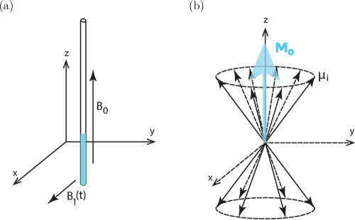
Figure 1.2: (a) NMR tube with sample oriented in a strong static magnetic field $B_{0}$ along the $z$-axis and time-dependent magnetic field $B_{1}(t)$ along the $x$-axis. (b) The number of spins precessing around the direction parallel to the field are more than the number antiparallel to the field direction, which creates a bulk magnetization $M_{0}$.

A nuclear spin with ${I}\neq 0$ when placed in a magnetic field of strength ${B_{0}}$ applied along the $z$-axis precesses as shown in Fig. 1.2(a). The Hamiltonian of interaction between the spin and the magnetic field is given by,

$${H}=-{\mu}.{B_{0}}\hat{z}=-\gamma_{n}\hbar{B_{0}}{I_{z}}=-\hbar\omega_{n}{I_{z}}$$ (1.21)

The spins precess about the $z$-axis with a characteristic frequency called Larmor frequency $\omega_{n}=-\gamma_{n}{B_{0}}$ (in rad s^-1) as shown in Fig. 1.2(b). The magnetic field ${B_{0}}$ is applied along the $z$-direction and all the quantum operators act in the subspace spanned by the magnetic quantum number $|m\rangle$ where $m=-{I},-{I}+1,\dots,{I}-1,{I}$. Under the action of the Hamiltonian ${H}$, the expectation values of the angular momentum operators in the plane perpendicular to the $z$-direction i.e. $\langle{I_{x}}\rangle$ and $\langle{I_{y}}\rangle$ show oscillatory behavior with time, with a frequency $\omega_{n}$, whereas $\langle{I_{z}}\rangle$ is stationary. The eigenvalues of the Hamiltonian ${H}$ are given by:

$$E_{m}=-m\hbar\omega_{n}$$ (1.22)

For a nucleus with spin $I$, there are $(2I+1)$ energy levels equally spaced by the amount $\hbar\omega_{n}$.

For an ensemble of identical nuclei which are not perfectly isolated from the environment and surrounded by the lattice is at a temperature $T$. The interactions of nuclei with the lattice lead to a thermal equilibrium state and the population of each energy level in this state is given by the Boltzmann distribution. For a two-level system $I=\frac{1}{2}$, with the population $n_{-}$ and $n_{+}$ of the $m=-\frac{1}{2}$ and $m=\frac{1}{2}$ levels, respectively

$$\frac{n_{-}}{n_{+}}=e^{-\hbar\omega_{n}/k_{B}T}$$ (1.23)

where $k_{B}$ is the Boltzmann constant and T is the absolute temperature of the ensemble. The Boltzmann factor $e^{-\hbar\omega_{n}/k_{B}T}$ for protons (${}^{1}{H}$) in a magnetic field of 14.1 Tesla at room temperature is very close to unity. The fractional difference of populations is about 1 part in $10^{5}$. This slight difference in the populations of $m=-\frac{1}{2}$ and $m=\frac{1}{2}$ levels cause the net magnetization along the $z$-direction. For $n$ spin-1/2 nuclei the thermal equilibrium magnetization is given by:

$${M_{0}}=\frac{\mu_{0}\gamma_{n}^{2}\hbar^{2}{B_{0}}}{4k_{B}T}$$ (1.24)

Since the Larmor frequency depends on the gyromagnetic ratio $\gamma_{n}$, each nucleus has its own characteristic Larmor frequency. Nuclear spins in a molecule are surrounded by the electronic environment, which leads to shielding of the magnetic field, the so called “chemical shift”, with the effective magnetic field being given by

$${B}_{{\rm eff}}={B_{0}}(1-\sigma_{0})$$ (1.25)

where $\sigma_{0}$ is the isotropic chemical shift tensor.

There are several terms in the nuclear spin Hamiltonian which encompass different spin-spin interactions such as the scalar coupling term ${{H_{J}}}$, the dipolar coupling term ${H_{DD}}$, and the quadrupolar coupling term ${H_{Q}}$. The scalar coupling interaction ${{H_{J}}}$ arise from the hyperfine interactions between the nuclei and local electrons. A pair of nuclei exhibit dipole-dipole interaction ${H_{DD}}$ by inducing local magnetic fields at the site of each other through space. In an isotropic liquid at room temperature, molecules tumble very fast, thus averaging the intramolecular dipolar coupling to zero. The quadrupolar coupling ${H_{Q}}$ is exhibited by nuclei with spin $>1/2$ which possess an asymmetric charge distribution [76].

Radio frequency field interaction and the resonance phenomenon:- The Larmor frequencies of the nuclear spins in a static magnetic field of a few Tesla are of the order of MHz. The transition between the different spin states can be induced by a radio frequency (rf) oscillating magnetic field [2].

$$\vec{B}_{rf}=2B_{1}cos(\omega_{rf}t+\phi)\hat{x},$$ (1.26)

where $\omega_{rf}$ is the frequency of the magnetic field and $\phi$ is the phase.

$$H_{rf}=-\mu.\vec{B}_{rf}=-\gamma_{n}\hbar{I_{x}}\left(2B_{1}cos(\omega_{rf}t+\phi)\right)$$ (1.27)

We can rewrite $\vec{B}_{rf}$ as a superposition of two fields rotating in opposite directions.

$$\vec{B}_{rf}=B_{1}(cos(\omega_{rf}t+\phi)\hat{x}+sin(\omega_{rf}t+\phi)\hat{y})+B_{1}(cos(\omega_{rf}t+\phi)\hat{x}-sin(\omega_{rf}t+\phi)\hat{y}),$$ (1.28)

For the simplicity, we assume $\phi=0$ and analyze Eq. 1.28 in a coordinate system that rotates around the static magnetic field at the frequency $\omega_{{rf}}$. In this rotating frame

$$\vec{B}_{rf}^{rot}=B_{1}\hat{x}+B_{1}(cos(2\omega_{rf}t)\hat{x}-sin(2\omega_{rf}t)\hat{y})$$ (1.29)

We can observe that one of the two components is now static and the other is rotating at twice the rf field frequency (which can be neglected) [77]. We can transform $H_{rf}$ into rotating frame using the unitary operator

$$U(t)=e^{i\omega_{n}t{I_{z}}/\hbar},$$ (1.30)

$H_{rf}^{rot}=U^{-1}H_{rf}U+i\hbar\dot{U}^{-1}U=-\hbar(\omega_{n}-\omega_{rf}){I_{z}}-\hbar\omega_{1}{I_{x}}$

where $\omega_{1}=\gamma_{n}B_{1}$. If the phase $\phi\neq 0$ then

$$H_{rf}^{rot}=-\hbar(\omega_{n}-\omega_{rf}){I_{z}}-\hbar\omega_{1}\{{I_{x}}cos\phi+I_{y}sin\phi\}.$$ (1.31)

The evolution of the quantum ensemble under the effective field in the rotating frame is described by

$$\rho_{rot}(t)=e^{-iH_{rf}^{rot}\ t}\rho_{rot}(0)e^{iH_{rf}^{rot}\ t},$$ (1.32)

where $\rho_{rot}(0)$ is density matrix of state at time $t$.

1.3 NMR quantum computing

In 1997, D. G. Cory and I. L. Chuang independently proposed a NMR quantum computer that can be programmed much like a quantum computer [78, 79]. Their computational model uses an ensemble quantum computer wherein the results of a measurement are the expectation values of the observables. This computational model can be realized by NMR spectroscopy on macroscopic ensembles of nuclear spins. Several quantum algorithms have been implemented on an NMR quantum computer such as the Grover search algorithm [30], realization of Shor algorithm [80], implementation of the Deutsch-Jozsa algorithm using noncommuting selective pulses [31] and many more till date. A qubit in an NMR quantum computer is realized by a spin-1/2 nucleus. The NMR spectrometer consists of a superconducting magnet which applies a high magnetic field in the $z$-direction and rf coils for exciting the spins and receiving the NMR signal from the relaxing spin ensemble. When the sample is placed in the magnetic field, the spins interact with the magnetic field, and energy levels split depending upon the size of the spin system. At room temperature, these energy levels are populated according to the Boltzmann distribution and thus the system is in a mixed state at thermal equilibrium. This poses a difficult challenge for quantum computing, which requires pure states as initial quantum states. This difficulty is circumvented in NMR quantum computing by creating a “pseudopure” state as an initial state, which mimics a pure state. Using the rf pulses and interaction between the spins, quantum gates are implemented and as a result of the computation the NMR signal was recorded which is an average magnetization the in $x$ and $y$ directions. This signal is directly proportional to the expectation values of some elements of the basis set of the qubits. With the application of rf pulses rotating individual spins, the expectation of all the elements in the basis set can be calculated. From these expectation values, we can reconstruct the density matrix. Further, recent developments in NMR in the area of control of spin dynamics via rf pulses makes it possible to implement quantum gates for NMR quantum computing with high fidelities. A nuclear spin is well separated from its environment due to which it exhibits long coherence times. Even with all these merits, one major limitation of liquid state NMR quantum computers is scalability. In the following sections, state initialization, implementation of quantum gates and measurement in NMR quantum computing are discussed.

1.3.1 NMR qubits

Consider an ensemble of $N$ spin-1/2 nuclei tumbling in a liquid and placed in a magnetic field $B_{0}$. The Hamiltonian $H$ of this system is given as

$$H=-\omega_{0}I_{z}$$ (1.33)

where $I_{z}=\sigma_{z}/2$. The eigenstate and eigenvalues of $H$ are $\{|0\rangle,|1\rangle\}$ and $\{\omega_{0}/2,-\omega_{0}/2\}$ respectively. The energy difference between the two levels is given by $\Delta E=\hbar\omega_{0}$ Hence such a two-level system acts as a single NMR qubit. For a system of $n$ interacting spins-1/2 in a magnetic field the Hamiltonian is given by:

$$H_{0}=\sum_{i=1}^{n}\omega_{i}I_{z}^{i}+2\pi\sum_{i<j}^{n}J_{ij}I^{i}.I^{j}$$ (1.34)

where $J_{ij}$ is the scalar coupling between the spins and $\omega_{i}$ is the Larmor frequency. If $|\omega_{i}-\omega_{j}|>>2\pi|j_{ij}|$ then the NMR qubits are weakly coupled and the Hamiltonian for such a system is

$$H_{0}=\sum_{i=1}^{n}\omega_{i}I_{z}^{i}+2\pi\sum_{i<j}^{n}J_{ij}I_{z}^{i}.I_{z}^{j}$$ (1.35)

1.3.2 Initialization

Any QIP task begins by initializing the system into a pure state. In NMR QIP, an $N$-qubit ensemble of spins at room temperature has a population distribution of energy levels given by the Boltzmann distribution [1]. All the energy levels are almost equally populated and the initial state is mixed. Under the high temperature approximation the initial state of the system is given by:

$$\rm\rho_{eq}\approx\frac{1}{2^{N}}(I+\epsilon\Delta\rho_{eq})$$ (1.36)

where $\rm I$ is an identity matrix of $\rm 2^{N}\times 2^{N}$, $\epsilon(\approx 10^{-5})$ is a purity factor and $\Delta\rho_{eq}$ is a deviation density matrix. The problem of pure states in NMR can be overcome by preparing a pseudopure state which is isomorphic to a pure state [78]. An ensemble of a pure state is given by $\rho_{pure}=|\psi\rangle\langle\psi|$ and the corresponding pseudopure state is given by

$$\rm\rho_{pps}=\frac{1-\epsilon}{2^{N}}I+\epsilon|\psi\rangle\langle\psi|$$ (1.37)

A pseudopure state in NMR can be prepared by several methods such as spatial averaging, temporal averaging and logical labelling; all based on the idea of preparing $\rm 2^{N}-1$ energy levels with equal population and with one energy level being more populated than the other energy levels as shown for two qubits in Fig.1.3.

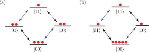
Figure 1.3: Populations of energy levels of a two-qubit system of a (a) thermal equilibrium state and (b) a pseudopure state.

To implement most quntum algorithms we need to create an entangled state. The power of quantum computers largely depends on entanglement. There has been a longstanding debate about the existence of entanglement in spin ensembles at high temperature as encountered in NMR experiments. There are two ways to look at the situation. Entangled states in such ensembles are obtained via unitary transformations on pseudopure states. If we consider the entire spin ensemble, given that the number of spins that are involved in the pseudopure state is very small compared to the total number of spins, it has been shown that the overall ensemble is not entangled [81, 82]. However, one can take a different point of view and only consider the subensemble of spins that have been prepared in the pseudopure state, and as far as these spins are concerned entanglement genuinely exists [83, 13]. The states that we have created in this thesis for our experiments are entangled in this sense, and hence may not be considered as entangled if one works with the entire ensemble. Therefore, one has to be aware and cautious about this aspect while dealing with these states. These states are sometimes referred to as being pseudoentangled.

Temporal averaging technique is based on the fact that quantum operations are linear and the observables measured in NMR are traceless. Experimentally, the temporal averaging scheme relies on adding the computational results of multiple experiments, where each experiment starts off with a different state preparation pulse sequence which permutes the populations [22]. For a two-spin system this technique begins with the density matrix

$\rho_{1}=\left(\begin{array}[]{cccc}p_{1}&0&0&0\\ 0&p_{2}&0&0\\ 0&0&p_{3}&0\\ 0&0&0&p_{4}\\ \end{array}\right)$

where $p_{1}$, $p_{2}$, $p_{3}$ and $p_{4}$ are populations of the normalized density operator $\rho_{1}$, with $\sum_{i=1}^{4}p_{i}=1$. $U_{1}$ and $U_{2}$ are operators constructed from controlled-NOT gates to obtain a state with the permuted populations:

$\rho_{2}=U_{1}.\rho_{1}.U_{1}^{\dagger}=\left(\begin{array}[]{cccc}p_{1}&0&0&0\\ 0&p_{3}&0&0\\ 0&0&p_{4}&0\\ 0&0&0&p_{2}\\ \end{array}\right)$

and

$\rho_{3}=U_{2}.\rho_{1}.U_{2}^{\dagger}=\left(\begin{array}[]{cccc}p_{1}&0&0&0\\ 0&p_{4}&0&0\\ 0&0&p_{2}&0\\ 0&0&0&p_{3}\\ \end{array}\right)$

Since the readout is linear with respect to the initial state, all three permuted density matrices are added to realize the pseudopure state $\rho=\rho_{1}+\rho_{2}+\rho_{2}$.

$\rho=\left(\begin{array}[]{cccc}3p_{1}&0&0&0\\ 0&p_{2}+p_{3}+p_{4}&0&0\\ 0&0&p_{2}+p_{3}+p_{4}&0\\ 0&0&0&p_{2}+p_{3}+p_{4}\\ \end{array}\right)$

Rewriting $\rho$

$\rho=\frac{p_{2}+p_{3}+p_{4}}{3}I+\frac{1}{3}\left(\begin{array}[]{cccc}4p_{1}-1&0&0&0\\ 0&0&0&0\\ 0&0&0&0\\ 0&0&0&0\\ \end{array}\right)$

$$\rho=\frac{1}{3}\left\{(1-p_{1})I+(4p_{1}-1)|00\rangle\langle 00|\right\}$$ (1.38)

where $\rho$ is the effective pure state corresponding to $|00\rangle$.

Spatial averaging technique uses rf pulses and pulsed field gradients (PFG) to prepare pseudopure states. The PFG kills the magnetization in the plane perpendicular to its applied direction by randomizing the spin magnetization in that plane and spin magnetization is retained only in the direction along which the PFGs are applied. For a two-qubit homonuclear system (homonuclear meaning spins belonging to the same species) the pseudopure state $\rho_{00}$ can be prepared from an initial thermal state using the following steps:

$\rm I_{z}^{1}$ +$\rm I_{z}^{2}$ ->[$\rm(\frac{\pi}{3})^{2}_{x}$] $\rm I_{z}^{1}$ + $\rm\frac{1}{2}I_{z}^{2}$ + $\rm\frac{\sqrt{3}}{2}I_{y}^{2}$

->[$\rm G_{z}$] $\rm I_{z}^{1}$ + $\rm\frac{1}{2}I_{z}^{2}$

->[$\rm(\frac{\pi}{4})^{1}_{x}$] $\rm\frac{1}{\sqrt{2}}I_{z}^{1}$-$\frac{1}{\sqrt{2}}I_{y}^{1}$ + $\rm\frac{1}{{2}}I_{z}^{2}$

->[$\rm\frac{1}{2J_{12}}$] $\rm\frac{1}{\sqrt{2}}I_{z}^{1}$ + $\rm\frac{1}{\sqrt{2}}2I_{x}^{1}I_{z}^{2}$ + $\rm\frac{1}{{2}}I_{z}^{2}$

->[$\rm(\frac{\pi}{4})^{1}_{-y}$] $\rm\frac{1}{\sqrt{2}}I_{z}^{1}$-$\frac{1}{\sqrt{2}}I_{x}^{1}$ + $\rm\frac{1}{\sqrt{2}}2I_{x}^{1}I_{z}^{2}$ + $\rm\frac{1}{{2}}2I_{z}^{2}I_{z}^{2}$ + $\rm\frac{1}{{2}}I_{z}^{2}$

->[$\rm G_{z}$] $\rm\frac{1}{2}(I_{z}^{1}$ + $\rm I_{z}^{2}+2I_{z}^{1}I_{z}^{2})$

where $I_{i}^{1}=\frac{1}{2}\sigma_{i}\otimes I$, $I_{i}^{2}=\frac{1}{2}I\otimes\sigma_{i}$, $\sigma_{i}$ with $i=x,y,z$ are Pauli matrices, ${J_{12}}$ is the scalar coupling constant between two spins and $\rm G_{z}$ is a PFG along the $z$-axis which kills all the magnetization in the $xy$-plane.

Logical labeling technique uses one qubit of $n$-qubits to label the state while the other $n-1$ qubits are placed in a pseudopure configuration [79]. To illustrate the logical labeling technique, let us consider a homonuclear three-qubit system at thermal equilibrium with its deviation density matrix

$\Delta\rho_{eq}={}\left(\begin{array}[]{cccccccc}3&0&0&0&0&0&0&0\\ 0&1&0&0&0&0&0&0\\ 0&0&1&0&0&0&0&0\\ 0&0&0&-1&0&0&0&0\\ 0&0&0&0&1&0&0&0\\ 0&0&0&0&0&-1&0&0\\ 0&0&0&0&0&0&-1&0\\ 0&0&0&0&0&0&0&-3\\ \end{array}\right)$

The relative population of the eigenstates are:

$\begin{array}[]{ccccccccc}{\text{ State}}&|000\rangle&|001\rangle&|010\rangle&|011\rangle&|100\rangle&|101\rangle&|110\rangle&|111\rangle\\ {\text{ Relative population}}&6&4&4&2&4&2&2&0\\ \end{array}$

Assuming the first qubit as a label, the first four eigenstates can be perceived as a two-qubit system with the label qubit in the state $|0\rangle$ and the other four eigenstates can be considered as a two-qubit system with the label qubit in the state $|1\rangle$. First a $\rm CNOT_{21}$ gate is applied (the second qubit being a control qubit and the first qubit being the target qubit) and then a $\rm CNOT_{31}$ gate is applied (the third qubit being the control qubit and the first qubit as the target qubit). The action of these two gates results in a final relative state population:

$\begin{array}[]{ccccccccc}{\text{ State}}&|000\rangle&|001\rangle&|010\rangle&|011\rangle&|100\rangle&|101\rangle&|110\rangle&|111\rangle\\ {\text{ Relative population}}&6&2&2&2&4&4&4&0\\ \end{array}$

The deviation part of the pseudopure state density matrix of the two qubits corresponding to label 0 is $\Delta\rho^{0}=4|00\rangle\langle 00|-I$ and corresponding to label 1 is $\Delta\rho^{1}=I-4|11\rangle\langle 11|$. In this thesis we will use the spatial averaging technique throughout for pseudopure state preparation.

1.3.3 Quantum gate implementation in NMR

Section 1.1.4 dealt with the mathematical description of quantum gates. This section will explain the physical implementation of unitary gates on an NMR quantum computer. In traditional NMR techniques, spin states are manipulated by using rf pulses or by free evolution under the internal nuclear spin interactions. It was shown in Section 1.2 that a spin which satisfies the resonance condition can be rotated about the $\hat{\phi}$ axis by applying an rf pulse along the $\hat{\phi}$ axis with high precession. Due to this, any quantum gate can be implemented in NMR with high fidelity using rf excitation pulses and interaction between the spins. The action of an on-resonance rf pulse with arbitrary phase $\hat{\phi}$ and duration $t_{p}$ is given by

$$(\theta)_{\phi}^{I}=exp(-i\omega_{1}t_{p}I_{\phi})=exp(-i\theta I_{\phi})$$ (1.39)

where $I_{\phi}=I_{x}cos(\phi)+I_{y}sin(\phi)$ and $\theta=\omega_{1}t_{p}$. The rf excitation pulse rotates a spin on-resonance with an angle $\theta$ along the $\hat{\phi}$ axis. A single-qubit gate can hence be implemented using this set of rotations. Some examples of NMR implementations of single-qubit gates are:

• Hadamard gate (H) can be implemented by a spin-selective pulse $\pi$ pulse along the $x$-axis and a $\frac{\pi}{2}$ pulse along the $y$-axis.

  

• Pauli-X gate (NOT gate) can be implemented by a single spin-selective $\pi$ pulse along the $x$-axis.

  

• Phase shift gate ($\rm R_{\phi}$) can be implemented by a single spin-selective $\phi$ pulse along the $z$-axis. However in NMR we can only apply rf pulses along an axis in the $xy$ plane, so a $\phi$ rotation along the $z$-axis is typically decomposed as a pulse cascade $(\frac{\pi}{2})_{x}(\phi)_{y}(\frac{\pi}{2})_{-x}$.

  

For the implementation of multi-qubit gates, we use the spin-spin interaction term in the Hamiltonian along with single-qubit gates. An NMR pulse sequence for the two-qubit CNOT gate is $(\frac{\pi}{2})_{-y}^{2}(\frac{\pi}{2})_{-z}^{1,2}\frac{1}{4J_{12}}{(\pi)^{1,2}_{y}}\frac{1}{4J_{12}}$ ${(\pi)^{1}_{y}}{(\frac{\pi}{2})_{y}}$; where $\frac{1}{J_{12}}$ denotes an evolution period under the coupling Hamiltonian.

1.3.4 Numerical techniques for quantum gate optimization

NMR quantum gates can be realized by the application of rf pulses and interactions between the spins. For heteronuclear coupled spins (where the spins under consideration belong to different nuclear species), due to the large Larmor frequency difference between the spins and the availability of multi-channel rf coils in the spectrometer hardware, it is easy to experimentally implement individual spin-selective rotations. However, for homonuclear spins (where the spins under consideration belong to the same nuclear species), it is difficult to selectively manipulate an individual spin, due to much smaller differences in the chemical shifts of the spins. The traditional way of exciting individual spins in NMR is by using a shaped pulse which is usually of long duration and results in a low experimental gate fidelity. To tackle this problem, one possible solution is optimization of quantum gates using numerical techniques. The most commonly used numerical optimization techniques are strongly modulated pulses, genetic algorithms and the gradient ascent pulse engineering (GRAPE) algorithm. This thesis mainly uses the GRAPE algorithm for gate optimization so it is discussed in detail, while the other techniques are discussed briefly.

Strongly modulated pulses (SMPs) is a procedure for finding high-power pulses that strongly modulate the dynamics of the system to precisely craft a desired unitary operation [84]. It uses the knowledge of the internal Hamiltonian and the form of the external Hamiltonian to generate the parameter values to determine the desired gate. SMPs make use of the Nelder-Mead Simplex algorithm [85] to minimize the quality factor by searching through the mathematical parameter space. It generates a control sequence as a cascade of rf pulses with fixed power, transmitter frequency, initial phase and pulse duration.

Genetic algorithms (GAs): These are stochastic search algorithms based on the concept of natural selection, a process which drives the biological evolution [86]. GAs modify the population of the individual solution at each step using the biological inspired operations such as selection, mutation, crossover etc. to evolve towards an optimal solution. At each step, the algorithm calculates the fitness of every individual solution and the algorithm runs until the desired fitness is achieved. In quantum information processing, GAs have been used to optimize quantum algorithms [87, 88, 89], for quantum entanglement [90] and for optical dynamical decoupling [91]. GAs have also been used to optimize the pulse sequences for unitary transformations on an NMR quantum information processor [27, 28].

Gradient ascent pulse engineering: To construct the desired unitary quantum gate $U_{tgt}$ using the GRAPE algorithm [92], we assume a closed system, with the propagator $U$ evolving under the Hamiltonian $H$ according to

$$\frac{d}{dt}U=-iHU.$$ (1.40)

Solving this equation leads to

$$U_{opt}=\prod_{j=1}^{N}U_{j}$$ (1.41)

and

$$U_{j}=exp\left\{-i\Delta t\left(H_{0}+\sum_{k=1}^{m}u_{k}(j)H_{k}\right)\right\}$$ (1.42)

where $H_{0}$ is the system Hamiltonian, $H_{k}$ is the rf control Hamiltonian and the control amplitudes $u_{k}$ are constant, i.e., during the $j$th step the amplitude $u_{k}(j)$ of the $kth$ control Hamiltonian is given by $u_{k}(j)$. If $T$ is the total pulse duration of the unitary gate then for simplicity the total time $T$ is discretized in $N$ equal steps and $\Delta t=T/N$. So, the problem is to find the optimal amplitudes $u_{k}(j)$ of the rf fields. The actual propagator $U_{opt}$ is identical to the desired operator $U_{D}$ when $||U_{opt}-U_{trg}||^{2}=0$ and in an optimization we will search for its minimum. Expanding further

$$||U-U_{D}||^{2} = Tr\{(U_{opt}-U_{tgt})^{\dagger}(U_{opt}-U_{tgt})^{\dagger}\}$$ (1.43)

$$= 2Tr\{I\}-2Re\{Tr\{U_{tgt}^{\dagger}U_{opt}\}\},$$

Hence our task is equivalent to maximization of

$$\Phi=Re\{Tr\{U_{tgt}^{\dagger}U_{opt}\}\}.$$ (1.44)

Further it is not necessary to exactly reproduce $U_{tgt}$. It serves equally well to reproduce the target operator up to a global phase factor $e^{i\phi}U_{tgt}$. Thus the task is equivalent to the maximization of

$$\Phi_{0}=|Tr\{U_{tgt}^{\dagger}U_{opt}\}|^{2}$$ (1.45)

This performance function increases if we choose

$u_{k}(j)$ -> $u_{k}(j)$ + $\epsilon$ $\frac{\delta\Phi_{0}}{\delta u_{k}(j)}$

where $\frac{\delta\Phi_{0}}{\delta u_{k}(j)}=2\Delta t{\rm Im}\{Tr\{U^{\dagger}_{tgt}U_{N}\dots U_{j+1}H_{k}U_{j}\dots U_{1}\}Tr\{U_{opt}^{\dagger}U_{tgt}\}\}$ and $\epsilon$ is a small step size.

The basic GRAPE algorithm consist of the following steps:

1. Guess initial controls $u_{k}(j)$.

2. Evaluate $\Phi_{0}$.

3. Evaluate $\frac{\delta\Phi_{0}}{\delta u_{k}(j)}$ and update the $m\times N$ control amplitudes $u_{k}(j)$.

4. With these as the new controls, iterate to step 2.

The algorithm is terminated if the change in the performance index $\Phi_{0}$ is smaller than a chosen threshold value.

Figure 1.4: Plot of rf pulse amplitude and phase with time, optimized with GRAPE for CSWAP gate.

In Fig. 1.4, plot of rf pulse amplitude and phase with time for GRAPE optimized CSWAP gate is shown with fidelity 0.9995. We used the three $\rm{}^{19}F$ spins of the trifluoroiodoethylene ($\rm C_{2}F_{3}I$) molecule as NMR sample. With GRAPE we can tackle errors due to rf inhomogeneity, off-set and flip angle by optimization.

1.3.5 Measurement in NMR

A conventional detection of the NMR signal is a so-called ensemble weak measurement, as the weak interaction of spins with radio-frequency coil does not change significantly the quantum states of the spins in the process of measuring the total spin magnetization. A direct projective measurement is not possible on NMR quantum computer. However, some experiments have been done to simulate projective measurements in NMR [93, 94].

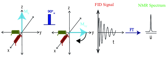
Figure 1.5: Rotation of Bulk magnetization using resonance. $B_{1}(t)$ applied in -x-direction for duration such that total rotation is $90^{\circ}$

As described in Section 1.2, when the nuclear spins are placed in the magnetic field $B_{0}$ along the $z$-axis, the average of the the magnetic moments $\mu$ of the nuclei at thermal equilibrium produces a bulk magnetization. With the application of rf pulses, this bulk magnetization is rotated from the $z$-axis to the $xy$ plane, where this rotated bulk magnetization precesses about the $z$-axis with a Larmor frequency $\omega_{0}$. The precessing bulk magnetization causes a change in magnetic flux in the rf coil which in turn produces a signal voltage as shown in Fig. 1.5. The recorded signal is proportional to the time rate of change of the magnetic flux linking an inductor that is a part of a tuned circuit. Due to relaxation processes with time the magnetization in the $xy$ plane decays and the resultant signal also decays with time (called free induction decay (FID)) as shown in Fig 1.5. If the quality factor of the coil is not too high, the recorded signal may be regarded as a time record of the instantaneous bulk magnetization that is transverse (in the $xy$-plane ) to the applied static field (which is in the $z$-axis). This rf signal is mixed down with a phase-sensitive detector, and the signal has both real ($x$) and imaginary ($y$) components. The time-domain signal of the transverse magnetization is given as

$$S(t)\propto Tr\left\{\rho(t)\sum_{k}(\sigma_{kx}+i\sigma_{ky})\right\}$$ (1.46)

where $\sum_{k}(\sigma_{kx}-i\sigma_{ky}$ is the detection operator, $\sigma_{kx}$ and $\sigma_{ky}$ are Pauli spin operators proportional to the $x$ and $y$ components of the magnetization due to $k^{th}$ spin and $\rho(t)$ is a reduced density operator which represents the average state of a single molecule [95]. The Fourier transform of Eq.1.46 gives the signal in the frequency domain which represent spectral lines at well-defined frequencies. These spectral lines are characteristic of the spin system used.

The state density matrix $\rho$, at any instant $t$, can be reconstructed by systematically measuring the NMR signal. This process of state reconstruction is called quantum state tomography (QST) [96, 95]. Any general normalized state state density matrix can be written as

$\rho=\left(\begin{array}[]{cc}a_{1}&a_{2}+ia_{3}\\ a_{2}-ia_{3}&1-a_{1}\\ \end{array}\right)$

The NMR signal is proportional to $\rho_{12}=a_{2}+ia_{3}$ and can be measured by measuring the intensity of the peaks from the real and imaginary parts of the spectra. The real intensity is proportional to $a_{2}$ and the imaginary intensity is proportional to $a_{3}$. For measuring $a_{1}$, a $\pi/2$ pulse along the $y$ axis is applied and the real intensity of the peak of spectra is proportional to $a_{1}$ [96]. The reconstruction of density matrix is discussed in detail in Chapter 2.

1.4 Evolution of quantum systems

Quantum systems which do not interact with the outside world are called closed systems. In reality however, no physical system is an entirely closed system, except perhaps the universe as a whole. Real systems suffer from unwanted interactions with their environment. These adverse interactions show up as noise in the quantum system. So, it is important to understand and control such a noise process in order to build realistic quantum information processors. The tools traditionally used by physicists for the description of open quantum systems are master equations, Langevin equations and stochastic differential equations. Another potent tool, which simultaneously addresses a broad range of physical scenarios is the mathematical formalism of quantum operations. With this formalism not only nearly closed systems which are weakly coupled to their environments but also the systems which are strongly coupled to their environments can be modeled. Quantum operations formalism is well adapted to describe discrete state change, that is, transformations between an initial state $\rho$ to final state $\rho{{}^{\prime}}$, without explicit reference to the passage of time [1].

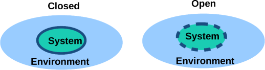
Figure 1.6: (a) Representation of a closed system; the circle around the system depicts no interaction between the system and environment. (b) Representation of an open system; the dashed circle around the system shows that the system and environment are interacting.

1.4.1 Closed quantum systems

The dynamics of a closed quantum system in a pure state is governed by the Schr$\rm\ddot{o}$dinger equation

$${i\hbar}\dfrac{\partial}{\partial t}{|\psi(x,t)\rangle}={H}_{sys}|\psi(x,t)\rangle$$ (1.47)

where $\psi(x,t)$ is the wave function, ${H}_{sys}$ the Hamiltonian, and $\hbar$ is Planck’s constant. In NMR closed systems, unitary evolution is governed by the Liouville-von Neumann equation

$$\dot{\rho}(t)=-\frac{i}{\hbar}[\ H_{sys},\rho(t)]\$$ (1.48)

The solution to Eq. (1.47) and Eq. (1.48) is given by

$$|\psi(t)\rangle = U(t)|\psi(0)\rangle$$ (1.49)

$$\rho(t) = U(t)\rho(0)U(t)^{\dagger}$$ (1.50)

where $|\psi(0)\rangle$ and $\rho(0)$ is a state of the system at time t=0 and

$$U(t)=Texp\left[-\frac{i}{\hbar}\int_{0}^{t}H_{sys}dt\right]$$ (1.51)

is a unitary operator. The dynamics of a closed quantum system can be described by a unitary transformation.

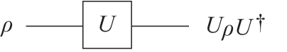
Figure 1.7: Model of closed quantum systems.

A model of a closed system is presented in Fig. 1.7 where the unitary transformation is represented as a box into which the input state $\rho$ enters and from which the output state $\rho^{{}^{\prime}}=U.\rho.U^{\dagger}$ exits.

1.4.2 Open systems

The standard approach for deriving the equations of motion for a system interacting with its environment is to expand the scope of the system to include the environment. The combined quantum system is then closed, and its evolution is governed by the Von Neumann equation.

$$\dot{\rho}_{tot}(t)=-\frac{i}{\hbar}[\ H_{tot},\rho_{tot}(t)]\$$ (1.52)

Here, we assume that the initial state of the total system can be written as a separable state $\rho_{tot}=\rho_{sys}\otimes\rho_{env}$ and $H_{tot}=H_{sys}+H_{env}+H_{int}$ is the total Hamiltonian, which includes the original system $H_{sys}$, the environment $H_{env}$, and interaction between the system and its environment Hamiltonian $H_{int}$. The solution to Eq.(1.52) is given by

$${\rho}_{tot}(t)=U(t)\rho_{tot}(0)U(t)^{\dagger}$$ (1.53)

Since we are interested in the dynamics of the principal system $\rho_{sys}$, we can extract the information about the system by taking the partial trace over the environment

$$\rho_{sys}=Tr_{env}[U(t)(\rho_{sys}\otimes\rho_{evn})U(t)^{\dagger}]$$ (1.54)

The most general trace-preserving and completely positive form of this evolution Eq.(1.52) is the Lindblad master equation for the reduced density matrix $\rho_{sys}=Tr_{env}[\ \rho_{tot}]\$. The Lindblad equation is the most general form for a Markovian master equation, and it is very important for the treatment of irreversible and non-unitary processes, from dissipation and decoherence to the quantum measurement process.

$$\dot{\rho_{sys}}(t)=-\frac{i}{\hbar}[\ H_{sys},\rho_{tot}(t)]\ +\sum_{i,\alpha}(L_{i,\alpha}\rho L_{i,\alpha}^{\dagger}+\frac{1}{2}\{L_{i,\alpha}^{\dagger}L_{i,\alpha},\rho\})$$ (1.55)

where the Lindblad operator $L_{i,\alpha}=\sqrt{k_{i,\alpha}}\sigma_{\alpha}^{(i)}$ acts on the $i$th qubit and describes decoherence, and $\sigma_{\alpha}^{(i)}$ denotes the Pauli matrix of the $ith$ qubit with $\alpha$= x, y, z. The constant $k_{i,\alpha}$ is approximately equal to the inverse of decoherence time.

If we consider only the first term on the right hand side of Eq.(1.55), we obtain the Liouville-von Neumann equation. This term is the Liouvillian and describes the unitary evolution of the density operator. The second term on the right hand side of the Eq.(1.55) is the Lindbladian and it emerges when we take the partial trace (a non-unitary operation) over the degrees of freedom of the environment. The Lindbladian describes the non-unitary evolution of the density operator and the Lindblad operators can be understood to represent the system contribution to the system-environment interaction.

Figure 1.8: Model of open quantum system consisting of two parts: the principal system and its environment.

In Fig. 1.8, we have a system in state $\rho_{sys}$ and environment in state $\rho_{env}$ which together form a closed system and sent into a box which represents the unitary operator on total system with the final state exiting the box being ${\cal E}(\rho)$. It is to be noted that ${\cal E}(\rho)$ may not be related by unitary transformation to the initial system state $\rho_{sys}$. The reduced state of the system alone can be obtained by taking a partial trace over the environment

$${\cal E}(\rho_{sys})=Tr_{evn}[U(\rho_{sys}\otimes\rho_{evn})U^{\dagger}]$$ (1.56)

Now, let us consider $\{|e_{k}\rangle\}$ to be an orthonormal basis for the state space of the environment and the initial state of the environment can be written as $\rho_{evn}=|e_{0}\rangle\langle e_{0}|$. Using Eq.(1.56), we get

$${\cal E}(\rho) = \sum_{k}\langle e_{k}|U[\rho\otimes|e_{0}\rangle\langle e_{0}|]U^{\dagger}|e_{k}\rangle$$ (1.57)

$$= \sum_{k}E_{k}\rho E_{k}^{\dagger},$$

where $E_{k}=\langle e_{k}|U|e_{0}\rangle$ is the Kraus operator. Eq.(1.57) is known as the operator-sum representation of $\cal{E}$. The operators $\{E_{k}\}$ are known as operation elements for the quantum operation $\cal E$, which satisfy

$$\sum_{k}E_{k}^{\dagger}E_{k}=I$$ (1.58)

1.4.3 Quantum noise channels

Quantum channels are convex-linear and completely positive trace preserving maps ${\cal E}$ which transform the initial state $\rho$ of a quantum system to another state ${\cal E}(\rho)$.

$${\cal E}:\rho \rightarrow {\cal E}(\rho)$$

$${\cal E}(\rho) = \sum_{k}E_{k}\rho E_{k}^{\dagger}$$ (1.59)

where $E_{k}$’s are the Kraus operators. Quantum channels can be used to describe the transformation occurring in the state of a system due to the system-environment interaction. The interaction of a single qubit with its environment can be described by three quantum noise channels which are: phase damping, generalized amplitude damping and depolarizing channel.

1.4.3.1 Generalized amplitude damping channel

The generalized amplitude damping channel describes the dissipative interactions between the system and its environment which cause interconversions of populations from ground state to excited states and vice versa at finite temperature [1]. For a single qubit, the Kraus operators for this channel are given by:

$$E_{1} = \sqrt{p}\left(\begin{array}[]{cc}1&0\\ 0&\sqrt{1-a}\\ \end{array}\right)$$ (1.62)

$$E_{2} = \sqrt{p}\left(\begin{array}[]{cc}0&\sqrt{a}\\ 0&0\\ \end{array}\right)$$ (1.65)

$$E_{3} = \sqrt{1-p}\left(\begin{array}[]{cc}\sqrt{1-a}&0\\ 0&1\\ \end{array}\right)$$ (1.68)

$$E_{4} = \sqrt{1-p}\left(\begin{array}[]{cc}0&0\\ \sqrt{a}&0\\ \end{array}\right)$$ (1.71)

where $E_{1}$ and $E_{2}$ operators are responsible for the process by which the population from its excited state will decay to its ground state, $E_{3}$ and $E_{4}$ operators are responsible for the reverse process in which populations convert from the ground state to the excited state, $p$ is the probability of finding population in the ground state at thermal equilibrium and $a=1-e^{-\gamma t}$ where ‘$\gamma$’ is the decay constant. The action of these Kraus operators on the density matrix $\rho$ is given by:

$${\cal E}(\rho) = E_{1}\rho E_{1}^{\dagger}+E_{2}\rho E_{2}^{\dagger},$$

$$\rho \rightarrow {\cal E}(\rho),$$

$$\left(\begin{array}[]{cc}\rho_{11}&\rho_{12}\\ \rho_{21}&\rho_{22}\\ \end{array}\right) \rightarrow \left(\begin{array}[]{cc}\rho_{11}^{{}^{\prime}}&\rho_{12}^{{}^{\prime}}\\ \rho_{21}^{{}^{\prime}}&\rho_{22}^{{}^{\prime}}\\ \end{array}\right),$$ (1.76)

where

$$\rho_{11}^{{}^{\prime}} = e^{-\gamma t}+p(1-e^{-\gamma t})\rho_{11}+p(1-e^{-\gamma t})\rho_{22},$$

$$\rho_{22}^{{}^{\prime}} = (1-p)(1-e^{-\gamma t})\rho_{11}+pe^{-\gamma t}\rho_{22},$$

$$\rho_{12}^{{}^{\prime}} = e^{-\gamma t/2}\rho_{12},$$

$$\rho_{21}^{{}^{\prime}} = e^{-\gamma t/2}\rho_{21}.$$

The Lindblad operator corresponding to the generalized amplitude damping channel is given as

$${\cal L}_{GD}=\sqrt{\frac{\gamma}{2}}\left(\begin{array}[]{cc}0&\sqrt{p}\\ \sqrt{(1-p)}&0\\ \end{array}\right)$$ (1.79)

In NMR, $\gamma$=1/ T₁ where T₁ is longitudinal relaxation time (explained in Section 1.4.5). The calculation becomes simple by assuming a high temperature approximation where $p=1/2$.

1.4.3.2 Phase damping channel

Phase damping (PD) channel is a non-dissipative channel, which mainly describes the loss of coherence without loss of energy. In this channel, the relative phase between $|0\rangle$ and $|1\rangle$ remains unchanged with some probability $p$ or is inverted $(\phi\rightarrow\phi+\pi)$ with probability $1-p$. If the system is in state $|0\rangle$ or $|1\rangle$, it will be unaffected by this channel. However, if it is in $|\psi\rangle=\alpha|0\rangle+\beta|1\rangle$ it gets entangled with the environment which destroys all the coherences but the probability of finding the qubit in state $|0\rangle$ or $|1\rangle$ does not change. The Kraus operators are given by:

$${\rm E_{1}} = \sqrt{p}\left(\begin{array}[]{cc}1&0\\ 0&1\\ \end{array}\right)$$ (1.82)

$${\rm E_{2}} = \sqrt{1-p}\left(\begin{array}[]{cc}1&0\\ 0&-1\\ \end{array}\right)$$ (1.85)

where $p=1-exp(-\lambda t)$ and $\lambda$ is the decay rate. The action of these operators transform the initial state $\rho$ to the final state ${\cal E}(\rho)$

$${\cal E}(\rho) = E_{1}\rho E_{1}^{\dagger}+E_{2}\rho E_{2}^{\dagger},$$ (1.86)

$$\rho \rightarrow {\cal E}(\rho),$$ (1.87)

$$\left(\begin{array}[]{cc}\rho_{11}&\rho_{12}\\ \rho_{21}&\rho_{22}\\ \end{array}\right) \rightarrow \left(\begin{array}[]{cc}\rho_{11}&exp(-\lambda t)\rho_{12}\\ exp(-\lambda t)\rho_{21}&\rho_{22}\\ \end{array}\right),$$ (1.92)

Under the action of the phase damping channel, the off-diagonal elements decay and diagonal elements remain unaffected.

The Lindblad operator corresponding to the phase damping channel is given as

$${\cal L}_{ph}=\sqrt{\frac{\lambda}{2}}\left(\begin{array}[]{cc}1&0\\ 0&-1\\ \end{array}\right)$$ (1.93)

In NMR, $\lambda$=1/T₂ where T₂ is the transverse relaxation time (explained in Section 1.4.6).

1.4.3.3 Depolarizing channel

Under the action of the depolarizing channel, the qubit remains intact with probability $1-p$ while with probability $p$ an identity type of noise occurs. The Kraus operator for the depolarizing channel is given by:

$${\rm E_{1}} = \sqrt{1-p}\left(\begin{array}[]{cc}1&0\\ 0&1\\ \end{array}\right),$$ (1.96)

$${\rm E_{2}} = \sqrt{\frac{p}{3}}\left(\begin{array}[]{cc}0&1\\ 1&0\\ \end{array}\right),$$ (1.99)

$${\rm E_{3}} = \sqrt{\frac{p}{3}}\left(\begin{array}[]{cc}0&-i\\ i&0\\ \end{array}\right),$$ (1.102)

$${\rm E_{4}} = \sqrt{\frac{p}{3}}\left(\begin{array}[]{cc}1&0\\ 0&-1\\ \end{array}\right),$$ (1.105)

where $p=1-exp(-dt)$ and $d$ is the decay rate. The action of these Kraus operators change the initial state $\rho$ to the final state ${\cal E}(\rho)$,

$$\rho \rightarrow {\cal E}(\rho),$$

$${\cal E}(\rho) = E_{1}\rho E_{1}^{\dagger}+E_{2}\rho E_{2}^{\dagger}+E_{3}\rho E_{3}^{\dagger}+E_{4}\rho E_{4}^{\dagger},$$

$$\left(\begin{array}[]{cc}\rho_{11}&\rho_{12}\\ \rho_{21}&\rho_{22}\\ \end{array}\right) \rightarrow \left(\begin{array}[]{cc}(\frac{2p}{3}+(1-\frac{4p}{3}))\rho_{11}&(1-\frac{4p}{3})\rho_{12}\\ (1-\frac{4p}{3})\rho_{21}&(\frac{2p}{3}+(1-\frac{4p}{3}))\rho_{22}\\ \end{array}\right),$$ (1.110)

We can further simplify Eq.(LABEL:dipolar) to

$${\cal E}(\rho)=\frac{\lambda}{2}I+(1-\lambda)\rho$$ (1.112)

where $\lambda=\frac{4p}{3}$ and $I$ is identity matrix.

The Lindblad operator corresponding to the depolarizing channel is

$${\cal L}_{D}=\sqrt{\frac{\delta}{3}}(\sigma_{x}+\sigma_{y}+\sigma_{z})$$ (1.113)

1.4.4 Nuclear spin relaxation

The bulk spin magnetization which is along the $z$-axis at thermal equilibrium, can be rotated to some other direction by the application of rf pulses. Over time the magnetization returns to the $z$-axis due to relaxation processes, which are explained by the famous Bloch equations, describing T₁ and T₂ relaxation processes.

1.4.5 Longitudinal relaxation

Longitudinal relaxation is the process by which the longitudinal component of spin magnetization returns to its equilibrium value, after a perturbation. In this process, energy is exchanged between the system of nuclear spins and its environment, which is called the lattice. This process is also known as spin-lattice relaxation. The phenomenological equation describing this process is of the form:

$$\frac{d{\text{M}}_{z}}{dt}=\frac{\text{M}_{0}-\text{M}_{z}}{\text{T}_{1}}$$ (1.114)

where T₁ is known as the longitudinal or the spin-lattice relaxation time and M₀ is the thermal equilibrium magnetization. The solution of the above equation is

$$\text{M}_{z}=\text{M}_{0}(1-e^{-t/\text{T}_{1}}),$$

when the M₀ is tilted to the $xy$ plane, then M${}_{z}(0)=0$.

For measuring T₁, the inversion recovery experiment is commonly used, where the spin magnetization is first inverted such that M${}_{z}(0)$=-M₀:

$$\text{M}_{z}=\text{M}_{0}(1-2e^{-t/\text{T}_{1}}).$$ (1.115)

1.4.6 Transverse relaxation

Transverse relaxation is the process that leads to the disappearance of the coherences namely the $xy$-magnetization. The phenomenological equation describing the decay of the transverse magnetization in the rotating frame can be written as:

$$\frac{d\text{M}_{x,y}}{dt}=-\frac{\text{M}_{x,y}}{\text{T}_{2}}$$ (1.116)

where T₂ is called the transverse relaxation time. The solution of this equation is

$$\text{M}_{x,y}=\text{M}_{0}e^{-t/\text{T}_{2}}$$ (1.117)

where $\text{M}_{0}$ is the initial value of the transverse magnetization after the application of a $90^{\circ}$ rf pulse.

1.4.7 Bloch-Wangness-Redfield relaxation theory

This relaxation model uses a quantum mechanical approach to describe the system parameters while the surrounding environment is described classically. The main limitation of this approximation is that at equilibrium the energy levels are predicted to be equally populated. The theory is formally valid only in the high-temperature limit. For finite temperatures, corrections are required to ensure that the correct equilibrium populations are reached. However these corrections are significant only in the case of very low temperatures [97, 98, 76, 99].

The von Neumann-Liouville equation, which describes the time evolution of the magnetic resonance phenomenon using spin density matrix $\rho(t)$ is given by

$$\frac{d\rho(t)}{dt}=-i[H_{0}+H_{1}(t),\rho(t)]$$ (1.118)

where $H_{0}$ is the time-independent part of the Hamiltonian which contains the spin Hamiltonian and $H_{1}(t)$ describes the time-dependent perturbations.

It is convenient to remove the explicit dependence on $H_{0}$ by rewriting the density operator $\rho(t)$ in a new reference frame, called the interaction frame:

$$\rho^{*}=exp(iH_{0}(t))\rho(t)exp(-iH_{0}(t))$$ (1.119)

It is possible to rewrite Eq.(1.118) in the interaction frame:

$$\frac{d\rho^{*}(t)}{dt}=-i[H^{*}_{1}(t),\rho^{*}(t)]$$ (1.120)

To solve Eq.(1.120) the following assumptions are required:

1. The ensemble average of $H_{1}^{*}(t)$ is zero.

2. $\rho^{*}(t)$ and $H_{1}^{*}(t)$ are not correlated, with this assumption it is possible to take the ensemble average of the fluctuations of the Hamiltonian and quantum states independently.

3. $\tau_{c}<<t<<2/R$, where $\tau_{c}$ is the correction time relevant for $H_{1}^{*}(t)$ and $R$ is the relevant relaxation rate constant.

4. For the system to relax towards the thermal equilibrium, $\rho^{*}(t)$ has to be replaced by $\rho^{*}(t)-\rho_{0}$, where $\rho_{0}$ is the density operator at equilibrium.

Using these assumption, the R.H.S in Eq.(1.120) can be replaced by an integral:

$$\frac{d\rho^{*}(t)}{dt}=-\int_{0}^{\infty}\overline{[H^{*}_{1}(t),[H^{*}_{1}(t-\tau),\rho^{*}(t)-\rho_{0}]]}d\tau$$ (1.121)

where the overbar represents the ensemble average. The third assumption allows the integral to run to infinity and with the assumption that the fluctuations of the Hamiltonian are not correlated with the density matrix, we can calculate the ensemble average over the stochastic Hamiltonian independently from $\rho^{*}(t)$.

For transforming Eq.(1.121) back in the lab frame, the stochastic Hamiltonian $H_{1}^{*}(t)$ has to be decomposed as the sum of the random functions of the spatial variable $F_{k}^{q}(t)$ and tensor spin operators $A^{q}_{k}$:

$$H_{1}(t)=\sum_{q=-k}^{k}(-1)^{q}F_{k}^{-q}(t)A_{k}^{q}$$ (1.122)

The tensor spin operators are chosen to be spherical tensor operators because of their transformations properties under rotations. For the Hamiltonians of interest in NMR spectroscopy, the rank of the tensor $k$ is one or two. These operators can be further decomposed as a sum of basis operators:

$$A_{k}^{q}=\sum_{p}A^{q}_{kp}$$ (1.123)

where the components $A^{q}_{kp}$ satisfy $[H_{0},A_{kp}^{q}]=\omega_{p}^{q}A_{kp}^{q}$. The transformation of $A_{k}^{q}$ in the interaction frame:

$$A_{k}^{q*}=exp(iH_{0}t)A_{k}^{q}exp(-iH_{0}t)=\sum_{p}A_{kp}^{q}exp(i\omega_{p}^{q}t)$$ (1.124)

Using Eq.(1.122) and Eq.(1.124) we can rewrite Eq.(1.121)

$$\frac{d\rho^{*}(t)}{dt} = -\sum_{q,q^{\prime}}\sum_{p,p^{\prime}}(-1)^{q+q^{\prime}}exp\{i(\omega_{p}^{q}+\omega^{q^{\prime}}_{p^{\prime}})t\}[A^{q^{\prime}}_{kp^{\prime}},[A^{q}_{kp},\rho^{*}(t)-\rho_{0}]]$$ (1.125)

$$\int_{0}^{\infty}\overline{F_{k}^{-q}(t)F_{k}^{-q}(t-\tau)}d\tau$$

If $q\neq-q$, the two random processes $F_{k}^{-q^{\prime}}(t)$ and $F_{k}^{-q^{\prime}}(t)$ are assumed to be statistically independent, due to which the ensemble average vanishes, unless $q^{\prime}=-q$.

$$\frac{d\rho^{*}(t)}{dt} = -\sum_{q=-k^{\prime}}^{k}\sum_{p,p^{\prime}}exp\{i(\omega_{p}^{q}-\omega^{q^{\prime}}_{p^{\prime}})t\}[A^{q}_{kp^{\prime}},[A^{q}_{kp},\rho^{*}(t)-\rho_{0}]]$$ (1.126)

$$\int_{0}^{\infty}\overline{F_{k}^{-q}(t)F_{k}^{-q}(t-\tau)exp(i\omega_{p}^{q}\tau)}d\tau$$

Further it is to be noted that terms in which $|\omega_{p}^{q}-\omega_{p}^{q}|>>0$ oscillate much faster than the typical time scales of the relaxation phenomena will not affect the evolution. In the absence of degenerate eigenfrequencies, terms in Eq.(1.126) do not vanish when $p=p^{\prime}$. Hence

$$\frac{d\rho^{*}(t)}{dt} = -\sum_{q=-k^{\prime}}^{k}\sum_{p}[A^{q}_{kp},[A^{q}_{kp},\rho^{*}(t)-\rho_{0}]]$$ (1.127)

$$\int_{0}^{\infty}\overline{F_{k}^{-q}(t)F_{k}^{-q}(t-\tau)exp(i\omega_{p}^{q}\tau)}d\tau$$

The terms $\overline{F_{k}^{-q}(t)F_{k}^{-q}(t-\tau)}$ are correlation functions. The real part of the integral in Eq.( 1.127) is the power spectral density function

$$j^{q}(\omega) = 2{\rm Re}\left\{\int_{0}^{\infty}\overline{F_{k}^{-q}(t)F_{k}^{-q}(t-\tau)exp(i\omega\tau)}\right\}$$

The imaginary part of the integral in Eq.( 1.127) is the power spectral density function

$$k^{q}(\omega) = {\rm Im}\left\{\int_{0}^{\infty}\overline{F_{k}^{-q}(t)F_{k}^{-q}(t-\tau)exp(i\omega\tau)}\right\}$$

In the high-temperature limit, the equilibrium density matrix is proportional to $H_{0}$. Thus, using Eq. (1.124), the double commutator $[[A^{-q}_{kp},A^{q}_{kp}],\rho_{0}]]=0$

$$\frac{d\rho^{*}(t)}{dt}=-\frac{1}{2}\sum_{q=-k}^{k}\sum_{p}[A^{-q}_{kp},[A^{q}_{kp},\rho^{*}(t)-\rho_{0}]]j^{q}(\omega^{q}_{p})+i\sum_{q=0}^{k}\sum_{p}[[A^{-q}_{kp},A^{q}_{kp}],\rho^{*}(t)]k^{q}(\omega^{q}_{p})$$ (1.128)

By transforming the above equation in lab frame

$$\frac{d\rho(t)}{dt}=-i[H_{0},\rho(t)]-i[\Delta,\rho(t)]-\hat{\Gamma}(\rho(t)-\rho_{0})$$ (1.129)

where the relaxation superoperator is

$$\hat{\Gamma}=-\frac{1}{2}\sum_{q=-k}^{k}\sum_{p}[A^{-q}_{kp},[A^{q}_{kp},]]j^{q}(\omega^{q}_{p})$$ (1.130)

$\Delta$ is the dynamic frequency shift operator that accounts for second-order frequency shifts of the resonance lines

$$\Delta=-\sum_{q=0}^{k}\sum_{p}[A^{-q}_{kp},A^{q}_{kp}]k^{q}(\omega^{q}_{p})$$ (1.131)

This term can be incorporated into the Hamiltonian to obtain the final result, known as master equation:

$$\frac{d\rho(t)}{dt}=-i[H_{0},\rho(t)]-\hat{\Gamma}(\rho(t)-\rho_{0})$$ (1.132)

In the calculation of relaxation rates it is often convenient to expand Eq.(1.132) in terms of the basis operators used to expand the density operator

$$\frac{db_{r}(t)}{dt}=\sum_{s}\{-i\Omega_{rs}b_{s}(t)-{\Gamma_{rs}}[b_{s}(t)-b_{s0}]\}$$ (1.133)

where $\Omega_{rs}$ are characteristic frequencies defined as

$$\Omega_{rs}=\frac{\langle\mathbf{B}_{r}|[H_{0},\mathbf{B}_{s}]\rangle}{\langle\mathbf{B}_{r}|\mathbf{B}_{s}\rangle}$$ (1.134)

$\Gamma_{rs}$ are the rate constant for relaxation between the operator $\mathbf{B}_{s}$ and $\mathbf{B}_{r}$

$$\Gamma_{rs} = \frac{\langle\mathbf{B}_{r}|\hat{\Gamma}\mathbf{B}_{s}\rangle}{\langle\mathbf{B}_{r}|\mathbf{B}_{s}\rangle}$$ (1.135)

$$= -\frac{1}{2}\sum_{q=-k}^{k}\sum_{p}\left\{\frac{\langle\mathbf{B}_{r}|[A^{-q}_{kp},[A^{q}_{kp},\mathbf{B}_{s}]]\rangle}{\langle\mathbf{B}_{r}|\mathbf{B}_{s}\rangle}\right\}j^{q}(\omega^{q}_{p})$$

and

$$b_{r}(t)=\frac{\langle\mathbf{B}_{r}|\rho(t)\rangle}{\langle\mathbf{B}_{r}|\mathbf{B}_{s}\rangle}$$ (1.136)

The diagonal elements $\Gamma_{rr}$ are auto-relaxation, while off-diagonal elements $\Gamma_{rs}$, are cross-relaxation rates.Because it is assumed that only terms satisfying $q=-q$ give non-zero contributions to Eq.(1.125), cross-relaxation can occur only between operators with the same coherence order. In addition, because of the secular approximation in Eq.(1.127), cross-relaxation between off-diagonal terms is forbidden in the absence of degenerate transitions. These two features give rise to a characteristic block shape in the relaxation superoperator, known as Redfield kite.

1.5 Decoherence suppression

The coherent superposition of states in combination with the quantization of observables, represents the one of the most fundamental features that mark the departure of quantum mechanics from the classical realm [100]. Quantum coherence in multi-qubit systems embodies the essence of entanglement and is an essential ingredient quantum information processing.A coherent quantum state in contact with environment loses coherence i.e. decoherence and entangle states are much more fragile to it. In NMR, $T_{2}$ gives an estimation of the decoherence time of the system and in liquid state NMR it is the of order of seconds. There is a longstanding debate on quantumness of NMR spin-systems states, the presence of nonzero discord in some of the states of NMR spin-systems indicates the intrinsic quantumness of nuclear spin systems even at high temperatures [83, 101].

Preserving quantum coherence is an important task in quantum information and different techniques have been developed to suppress decoherence. These techniques are broadly categorized as quantum error correction [102], decoherence free subspaces [103, 104] and dynamical decoupling (DD) methods [105, 106]. In particular, the DD technique is an important technique which suppresses the decoherence by eliminating the system-bath coupling. The idea comes from spin-echo pulses in NMR where static but nonuniform couplings can be compensated for perfectly by a single $\pi$ pulse in the middle of the time interval [107]. The idea of the spin echo was expanded to suppress dynamic interactions with the environment by using periodic $\pi$ pulses or by periodic Carr-Purcell cycles. The Carr-Purcell sequence was further modified to compensate errors due to $\pi$ pulses and Carr-Purcell-Meiboom-Gill sequence (CPMG) was devised [108]. A more sophisticated technique namely the Uhrig dynamical decoupling sequence was devised and it was shown that instead of applying $\pi$ pulses at equal intervals of time if $\pi$ pulses are applied at unequal intervals of time then the sequence shows better preservation [109]. One of the advantages of the DD technique is that no extra qubits are required unlike other techniques. Most DD preserving sequences are constructed to take care of dephasing type noise. In NMR language, T₂ type relaxation is considered and noise due to T₁ relaxation is ignored.

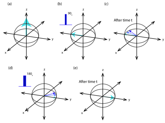
Figure 1.9: Evolution of the bulk magnetization under Hahn echo sequence. (a) Initially thermal equilibrium bulk magnetization in $z$ direction is represented by an arrow. (b) Bulk magnetization rotated to $-y$ axis using $90^{\circ}$ pulse, (c) A delay of time $t$ is given and arrows represent different spins, (d) $180^{\circ}$ is applied to spins due to which a spin precessing fast will fall behind a spin precessing slowly, and (e) after time $t$, all the spins are in the same direction.

1.5.1 Hahn echo

This technique was constructed by E. L. Hahn for suppressing time-independent noise in a system of isolated spins [107]. In an NMR setup, the static magnetic field $B_{0}$ along the $z$ axis has a spatial inhomogeneity due to which different spins in the ensemble experience different magnetic field and hence precess with different Larmor frequencies (which cause spin dephasing). To tackle this problem Hahn devised the spin-echo sequence as shown in Fig. 1.9. Initially at thermal equilibrium the bulk magnetization is in the $z$ direction. With the application of an rf pulse, a $(\pi/2)_{x}$ rotation is applied to the bulk magnetization. After time $t$ a spin experiencing a greater magnetic field will be ahead of a spin which experiences a smaller magnetic field as shown in Fig. 1.9(c). Then, a $\pi$ pulse is applied due to which the slow moving spins come close to and the fast moving spins move away from the $y$ axis. After time $t$ all the spins precess in the same direction as shown in Fig. 1.9(e).

1.5.2 CPMG DD sequence

In the Carr-Purcell(CP) sequence a series of rf pulses are applied: the first pulse flips the magnetization through $\frac{\pi}{2}$ angle with a $\frac{\pi}{2}$ pulse along the $x$-axis, and the following train of equidistant pulses flip the magnetization through $\pi$ with the $\pi$ pulse along the $x$-axis [110]. In the actual application of the Carr and Purcell method for the measurement of long relaxation times, it was found that the amplitude adjustment of the $\pi$ pulses was critical. This is because a small deviation from the exact $\pi$ value gives a cumulative error in the results. In the Carr-Purcell-Meiboom-Gill(CPMG) sequence: the first pulse flips the magnetization through $\frac{\pi}{2}$ angle with a $\frac{\pi}{2}$ pulse along a $y$-axis, and a series of $\pi$ pulses along the $x$ axis are applied at times $t=\frac{(2n+1)\tau}{2}$, $(n=0,1,2\dots)$. The CPMG sequence was able to suppress the time-dependent noise.

Figure 1.10: Pulse sequence of CPMG DD sequence for a cycle of duration $T$ and in one cycle eight pulses are applied; filled bars represent $\pi$ rotation pulses and $\tau$ is the duration between two consecutive $\pi$ pulses.

In the CPMG sequence a train of equidistant $\pi$ pulses are applied on a qubit. In Fig. 1.10 a train of eight pulses are applied in one cycle of duration $T$. The more the number of pulses in a cycle, the better is the decoherence suppression.

1.5.3 Uhrig DD sequence

The Uhrig DD (UDD) sequence is an optimal DD scheme and was first constructed by Uhrig for a pure dephasing spin-boson model [109], which uses $N$ $\pi$ pulses applied at time intervals $T_{j}$

$$T_{j}=Tsin^{2}\frac{j\pi}{2(N+1)}\ \ \ \text{for}\ \ \ j=1,2,\dots N,$$ (1.137)

to eliminate the dephasing up to order $O(T^{N+1})$; hence the UDD technique suppresses low-frequency noise. The CPMG sequence is a UDD sequence of order $N=2$. If for an interval of duration $T$, two $\pi$ pulses are applied the CPMG sequence, it will eliminate dephasing up to order $O(T^{3})$. Further, the proof of the universality of the UDD in suppressing the pure dephasing or the longitudinal relaxation of a qubit coupled to a generic bath has been given [111].

Figure 1.11: Pulse sequence for UDD sequence for a cycle time of $T$ and the number of $\pi$ pulses in one cycle of sequence is eight. Filled bars represent $\pi$ rotation pulses.

Yang and Liu considered ideal UDD pulse sequences for a Hamiltonian of the form

$$\hat{H}=\hat{C}+\hat{\sigma}_{z}\otimes\hat{Z},$$ (1.138)

where $\hat{\sigma_{z}}$ is the qubit Pauli matrix along the $z$-direction, and $\hat{C}$ and $\hat{Z}$ are bath operators. This Hamiltonian describes a pure dephasing model as it contains no qubit flip processes and therefore leads to no longitudinal relaxation but only transverse dephasing. Defining two unitary operator $U^{(N)}_{\pm}$ as follows:

$$U^{(N)}_{\pm}(T) = e^{-i[C\pm(-1)^{N}Z](T-T_{N})}$$ (1.139)

$$\times\ e^{-i[C\pm(-1)^{(N-1)}Z](T_{N}-T_{N-1})}\cdots$$

$$\times\ e^{-i[C\mp Z](T_{2}-T_{1})}e^{-i[C\pm Z]T_{1}}$$

Yang and Liu proved that for $T_{j}$ satisfying Eq. (1.137), we must have

$$\left(U^{(N)}_{-}\right)^{\dagger}U^{(N)}_{+}=1+O(T^{N+1}),$$ (1.140)

i.e., the product of $\left(U^{(N)}_{-}\right)^{\dagger}$ and $U^{(N)}_{+}$ differs from unity only by the order of $O(T^{N+1})$ for sufficiently small $T$ [111]. In Fig.1.11, eight $\pi$ pulses are applied with UDD timing preserving qubit coherence up to order $O(T^{9})$, whereas the CPMG sequence in Fig.1.10 is able to preserve coherences up to order $O(T^{3})$.

1.5.4 Super-Zeno Scheme

The super-Zeno scheme is an algorithm for suppressing the transitions of a quantum mechanical system, initially prepared in a subspace $\cal{P}$ of the full Hilbert space of the system, to outside this subspace by subjecting it to a sequence of unequally spaced short-duration pulses [60]. These durations were calculated numerically the leakage probability from subspace $\cal{P}$ to its orthogonal subspace was minimized, and surprisingly the durations matched with Eq.(1.137). This scheme is experimentally implemented in Chapter3. This scheme efficiently cancels all the noise affecting the state, and the preservation is up to the order $O(T^{N+1})$, where $N$ denotes the number of inverting pulses $J$ which are applied. The construction of this inverting pulse $J$ depends the on subspace $\cal{P}$.

1.5.5 Nested Uhrig dynamical decoupling

The nested Uhrig dynamical decoupling (NUDD) scheme is an extension of the super-Zeno scheme for the case where instead of a state, only the subspace to which the state belongs is known [64]. For protecting an unknown state in a known subspace, nesting of UDD protecting sequences are done in a a smart way such that these nesting of layers cancels all the possible interactions which affect states belonging to the $\cal{P}$ subspace. The inverting pulses of each layer are constructed on the basis of subspace to be protected, and these inverting pulses are applied at the UDD time points given by Eq.(1.137). The NUDD scheme is very sensitive to the nesting of layers, and for the time interval $T$ with $N$ pulses in each layer, protection is achieved of $O(T^{N+1})$. The NUDD scheme is discussed in detail in Chapter 4.

1.6 Organization of the thesis

This thesis deals with the estimation of experimentally prepared quantum states and protection of these states using different decoupling strategies. The thesis is organized as follows: Chapter 2 demonstrates the utility of the Maximum Likelihood (ML) estimation scheme to estimate quantum states on an NMR quantum information processor. We experimentally prepare separable and entangled states of two and three qubits, and reconstruct the density matrices using both the ML estimation scheme as well as standard quantum state tomography (QST). Further, we define an entanglement parameter to quantify multiqubit entanglement and estimate entanglement using both the QST and the ML estimation schemes. Chapter 3 demonstrates the efficacy of the super-Zeno scheme for the preservation of a state by freezing state evolution (one-dimensional subspace protection) and subspace preservation by preventing leakage of population to an orthogonal subspace (two-dimensional subspace protection). Both kinds of protection schemes are experimentally demonstrated on separable as well as on maximally entangled two-qubit states. Chapter 4 demonstrates the efficacy of NUDD scheme for the protection of arbitrary states of the known subspace. Chapter 5 focuses on extending the lifetime of time-invariant discord using dynamical decoupling schemes. Chapter 6 is based on modeling the noise and experimental protection of a three-qubit system using dynamical decoupling. Chapter 7 summarizes the work done in this thesis and discusses the future prospects.

Chapter 2 State tomography on an NMR quantum information processor via maximum likelihood estimation

2.1 Introduction

Classically, a state is assigned to a physical system by determining the phase space point corresponding to the configuration of the system and measuring the relevant system parameters in a non-invasive manner. For quantum systems, non-invasive measurements are not possible and therefore an ensemble of identically prepared systems are required for state estimation. The quantum state cannot be known from a single measurement and the ‘no-cloning’ theorem renders impossible the possibility of making several copies of the state and using them to make different measurements on the same state. Quantum state estimation is hence intrinsically a statistical process [112, 113]. In quantum information and experimental quantum computing, the complete estimation of a quantum state from a set of measurements on a finite ensemble is a hot topic of research. Several schemes have been proposed and implemented for quantum state estimation [114, 115, 116]. Due to the finite size of ensembles, a physical situation may even have two different candidate states and there is always some ambiguity associated with the estimated state. Such uncertainties and ambiguities, if not treated properly can lead to a self-contradictory estimation, where the estimated state is not even a valid quantum state. The density operator provides a convenient way to describe a quantum system whose state is not a pure state. It is a positive, Hermitian operator with $Tr[\rho]=1$ and $Tr[\rho^{2}]\leq 1$. For a pure ensemble $Tr[\rho^{2}]=1$ and for a mixed ensemble $Tr[\rho^{2}]<1$. In NMR, the quantum state tomography (QST) of $n$ coupled spins is carried out by measuring free induction decays (FIDs) after applying a set of preparatory pulses and applying a Fourier transformation to obtain spectral lines [117, 118, 96, 95]. Fitting these spectral lines, yields complex amplitudes at well defined frequencies which are characteristic of the spin system. These complex amplitudes are measured experimentally for each pulse in the preparatory pulse set. Using this experimental data a state density matrix is reconstructed. However, the reconstructed density matrix with the standard QST procedure leads to an unphysical density matrix i.e., some eigenvalues could turn out to be negative. This unphysical density matrix makes no sense, as even if there are experimental errors they should be within the space of allowed density operators. An ad hoc way to circumvent this problem is to add a multiple of identity to this density matrix so that the eigenvalues are positive. A scheme that redresses this issue of reconstructed density matrices that are unphysical, is the maximum-likelihood (ML) estimation scheme, which obtains a positive definite estimate for the density matrix by optimizing a likelihood functional that links experimental data to the estimated density matrix along with the constraint that the density matrix should be positive at every point of optimization  [57, 58, 119].

The ML estimation scheme begins with a guess quantum state and improves the estimate based on the measurements made; the more the number of measurements, the better is the state estimate.

This issue of unphysical density matrices was first pointed out in quantum optics where state reconstruction based on the inversion of measured data could not guarantee the positive definiteness of the reconstructed density matrix. Hence an algorithm for quantum-state estimation based on the maximum-likelihood (ML) estimation was proposed [56, 120]. A general method proposed for quantum state estimation based on the ML approach can be applied to multi-mode radiation fields as well as to spin systems [55]. An ensemble of spin-$\frac{1}{2}$ particles was observed repeatedly using Stern-Gerlach devices with varying orientations and the state of an ensemble was reconstructed via ML estimation [121] . A simple iterative algorithm for ML estimation of the quantum state was derived [122]. A tomographic protocol for a two-qubit system was recently constructed based on the measurement of 16 generalized Pauli operators which is maximally robust against errors [123]. A refined iterative ML algorithm was also proposed to reconstruct a quantum state and applied to the tomography of optical states and entangled spin states of trapped ions [124]. Other quantum state estimation algorithms include Bayesian mean estimation [125], least-squares inversion [126], numerical strategies for state estimation [126] and linear regression estimation [127]. If the size of the ensemble is infinite, the estimation procedure will yield the unique true quantum state of the system. However, such an ensemble is never achievable in any laboratory setting, as one can only perform measurements on a finite ensemble. As a result, the estimated state will be different from the true state and depends on the details of the estimation procedure. Quantum state reconstruction on a finite number of copies of a quantum system with informationally incomplete measurements, as a rule, does not yield a unique result. A reconstruction scheme was derived where both the likelihood and the von Neumann entropy functionals were maximized (MLME) in order to systematically select the most-likely estimator with the largest entropy, that is, the least-bias estimator, was consistent with a given set of measurement data. This MLME estimation protocol was applied to time-multiplexed detection tomography and light-beam tomography [128, 129].

In this chapter, the utility of the ML estimation scheme has been demonstrated to perform quantum state estimation on an NMR quantum information processor. Separable and entangled states of two and three qubits are experimentally prepared, and the density matrices are reconstructed using both the standard QST and the ML estimation schemes. For the quantification of entanglement in multiqubit systems an entanglement parameter is defined and it is shown that the standard QST method overestimates the residual state entanglement at a given time, while the ML estimation method gives a correct estimate of the amount of entanglement present in the state.

2.1.1 NMR quantum state tomography

The basic aim of quantum state tomography (QST) is to completely reconstruct an unknown state via a set of measurements on an ensemble of identically prepared states. Any density matrix $\rho$ of $n$ qubits in a $2^{n}$-dimensional Hilbert space can be uniquely determined using $4^{n}-1$ independent measurements and the state of the system as described by its density operator $\rho$ can be reconstructed by performing a set of projective measurements on multiple copies of the state [130, 29]. Determining all the elements of $\rho$ would involve making repeated measurements of the same state in different measurement bases, until all the elements of $\rho$ are determined  [131, 132, 119].

In NMR we cannot perform projective measurements and instead measure the expectation values of certain fixed operators over the entire ensemble. Therefore, we rotate the state via different unitary transformations before performing the measurement to collect information about different elements of the density matrix  [29]. The standard tomographic protocol for NMR uses the Pauli basis to expand an $n$ qubit $\rho$,

$$\rho=\sum_{i=0}^{3}\sum_{j=0}^{3}...\sum_{k=0}^{3}c_{ij...k}\sigma_{i}\otimes\sigma_{j}\otimes....\sigma_{k}$$ (2.1)

where $c_{00...0}=1/2^{n}$ and $\sigma_{0}$ denotes the $2\times 2$ identity matrix while $\sigma_{1}$, $\sigma_{2}$ and $\sigma_{3}$ are standard Pauli matrices. The measurements of expectation values allowed in an NMR experiment combined with unitary rotations leads to the determination of the coefficients $c_{ij..k}$.

In an NMR experiment, we measure the signal induced in the detection coils while the nuclear spins precess freely in a strong applied magnetic field. This signal is called the free induction decay (FID) and is proportional to the time rate of change of magnetic flux. This time-domain signal can be expressed in terms of the expectation values of the transverse magnetization [95]:

$$S(t)\propto\mbox{Tr}\left\{\rho(t)\sum_{k}(\sigma_{kx}-i\sigma_{ky})\right\}$$ (2.2)

where $\sigma_{kx}$ and $\sigma_{ky}$ are the Pauli spin operators proportional to the $x$ and $y$ components of the magnetization of the $k^{th}$ spin and $\rho(t)$ is the instantaneous density operator at time $t$ during the FID. The recorded signal represents an average over a large number of identical molecules of the sample.

The transformation of an initial density operator $\rho_{0}$ under applied pulses $U_{P}$ and under free-evolution Hamiltonian $H$ for time $t$ is given by:

$$\rho(t)=e^{-iHt}U_{P}\rho_{0}U_{P}^{\dagger}e^{iHt}.$$ (2.3)

Then Eq.(2.2) reduces to

$$S_{p}(t)\propto\mbox{Tr}\left\{e^{-iHt}U_{P}\rho_{0}U_{P}^{\dagger}e^{iHt}\sum_{k}(\sigma_{kx}-i\sigma_{ky})\right\},$$ (2.4)

using the linearity of the trace and its invariance with respect to cyclic permutation of the operators, we can write

$$S_{p}(t)\propto\mbox{Tr}\left\{\rho_{0}U_{P}^{\dagger}e^{iHt}\sum_{k}(\sigma_{kx}-i\sigma_{ky})e^{-iHt}U_{P}\right\}$$ (2.5)

In NMR spectroscopy, the initial density operator $\rho_{0}$ is known and it represents the thermal equilibrium state then from the signal we can determine the Hamiltonian. However in state tomography the reverse is true i.e. the Hamiltonian is known and the state $\rho_{0}$ is unknown. The Hamiltonian of $n$ weakly coupled spins-$\frac{1}{2}$ is given by,

$$H=-\sum_{k=1}^{n}\omega_{k}I_{kz}+2\pi\sum_{k=2}^{n}\sum_{j=1}^{k-1}J_{jk}I_{jz}I_{kz}$$ (2.6)

where $\omega_{k}/2\pi$ is the Larmor frequency of the $k$th spin, and $J_{jk}$ is the spin-spin coupling constant between $j$th and $k$th spins.

For a single spin system, the Hamiltonian $H_{1}$ consists of a Zeeman term only, which can be written as

$$H_{1}=\frac{1}{2}\omega\sigma_{z}$$ (2.7)

where $\omega$ is the Larmor frequency of the nuclear spin in the external magnetic field. Then, the NMR signal can be written as

$$S^{1}_{p}(t)\propto\mbox{Tr}\left\{\rho_{0}U_{P}^{\dagger}e^{i\frac{1}{2}\omega\sigma_{z}t}\sum_{k}(\sigma_{kx}-i\sigma_{ky})e^{-i\frac{1}{2}\omega\sigma_{z}t}U_{P}\right\}$$ (2.8)

Without applying any pulse i.e. $U_{p}=I$, the NMR signal is

$$S^{1}_{I}(t)\propto\left\{\mbox{Tr}[\rho_{0}\sigma_{x}]-i\mbox{Tr}[\rho_{0}\sigma_{y}]\right\}e^{i\omega t}.$$ (2.9)

after applying $90^{o}$ pulse along $x$ i.e. $U_{p}=90^{o}_{x}$, the NMR signal is

$$S^{1}_{X}(t)\propto\left\{\mbox{Tr}[\rho_{0}\sigma_{x}]-i\mbox{Tr}[\rho_{0}\sigma_{z}]\right\}e^{i\omega t}.$$ (2.10)

after applying $90^{o}$ pulse along $y$ i.e. $U_{p}=90^{o}_{y}$, the NMR signal can be written as

$$S^{1}_{Y}(t)\propto\left\{\mbox{Tr}[\rho_{0}\sigma_{z}]-i\mbox{Tr}[\rho_{0}\sigma_{y}]\right\}e^{i\omega t}.$$ (2.11)

Applying a Fourier transformation on Eq.(2.9, 2.10 and 2.11) then the ensemble average of operators $\sigma_{x}$, $\sigma_{y}$ and $\sigma_{z}$ can be obtained

$$\langle\sigma_{x}\rangle = c\leavevmode\nobreak\ {\rm avg}({\rm Re}[S_{I}(\omega)],{\rm Re}[S_{X}(\omega)]),$$ (2.12)

$$\langle\sigma_{y}\rangle = c\leavevmode\nobreak\ {\rm avg}(-{\rm Im}[S_{I}(\omega)],-{\rm Im}S_{Y}(\omega)]),$$ (2.13)

$$\langle\sigma_{z}\rangle = c\leavevmode\nobreak\ {\rm avg}(-{\rm Im}[S_{X}(\omega)],{\rm Re}[S_{Y}(\omega)]).$$ (2.14)

Where ${\rm avg}(a,b)$ means an average of $a$ and $b$. The factor $c$ depends on the experimental details such as the receiver gain and the number of spins. After determining the factor $c$, the density operator of a single spin can be estimated as

$$\rho=\frac{1}{2}I+\langle\sigma_{x}\rangle\sigma_{x}+\langle\sigma_{y}\rangle\sigma_{y}+\langle\sigma_{z}\rangle\sigma_{z}$$ (2.15)

For a two-spin system, the Hamiltonian can be written as

$$H_{2}=\frac{1}{2}\omega_{1}\sigma_{1z}+\frac{1}{2}\omega_{2}\sigma_{2z}+\frac{\pi}{2}J_{12}\sigma_{1z}\sigma_{2z}$$ (2.16)

where $J_{12}$ is the scalar coupling constant. After inserting $H_{2}$ in Eq.(2.5) and solving few steps the NMR signal due to spin 1 can be written as

$$S_{P,1}(t)\propto\frac{1}{2}(e^{i(\omega_{1}-\pi J_{12})t},e^{i(\omega_{1}+\pi J_{12})t})\times\left(\begin{array}[]{cc}1&1\\ 1&-1\\ \end{array}\right)\left(\begin{array}[]{c}\mathrm{Tr}\{\rho_{0}\tilde{\sigma}_{1-}\}\\ \mathrm{Tr}\{\rho_{0}\tilde{\sigma}_{1-}\tilde{\sigma}_{2z}\}\\ \end{array}\right)$$ (2.17)

Where $\tilde{\sigma}_{1-}=U_{P}^{\dagger}(\sigma_{1x}-i\sigma_{1y})U_{P}$. Fourier transformation of $S_{P,1}(t)$ leads to,

$$\left(\begin{array}[]{c}\bar{S}_{P,1}(\omega_{1}-\pi J_{12})\\ \bar{S}_{P,1}(\omega_{1}+\pi J_{12})\\ \end{array}\right)\propto\frac{1}{2}\left(\begin{array}[]{cc}1&1\\ 1&-1\\ \end{array}\right)\left(\begin{array}[]{c}\mathrm{Tr}\{\rho_{0}\tilde{\sigma}_{1-}\}\\ \mathrm{Tr}\{\rho_{0}\tilde{\sigma}_{1-}\tilde{\sigma}_{2z}\}\\ \end{array}\right)$$ (2.18)

Similarly for spin 2,

$$\left(\begin{array}[]{c}\bar{S}_{P,2}(\omega_{2}-\pi J_{12})\\ \bar{S}_{P,2}(\omega_{2}+\pi J_{12})\\ \end{array}\right)\propto\frac{1}{2}\left(\begin{array}[]{cc}1&1\\ 1&-1\\ \end{array}\right)\left(\begin{array}[]{c}\mathrm{Tr}\{\rho_{0}\tilde{\omega}_{2-}\}\\ \mathrm{Tr}\{\rho_{0}2\tilde{\omega}_{1z}\tilde{\omega}_{2-}\}\\ \end{array}\right)$$ (2.19)

The density matrix of a two-spin system can be expanded in terms of Pauli basis operators $I_{1}\otimes I_{2}\dots\sigma_{1z}\otimes\sigma_{2z}$, as follows:

$$\rho = \frac{1}{4}(I_{1}\otimes I_{2}+\langle\sigma_{1x}\otimes I_{2}\rangle\sigma_{1x}\otimes I_{2}+\dots$$ (2.20)

$$+\langle\sigma_{1z}\otimes\sigma_{2y}\rangle\sigma_{1z}\otimes\sigma_{2y}+\langle\sigma_{1z}\otimes\sigma_{2z}\rangle\sigma_{1z}\otimes\sigma_{2z})$$

and for the estimation of $\rho$ we need to calculate the expectation values $\langle\sigma_{1x}\otimes I_{2}\rangle$,$\dots$, $\langle\sigma_{1z}\otimes\sigma_{2z}\rangle$. From the NMR spectra we can calculate the peaks intensities i.e. $\bar{S}_{P,1}$ and $\bar{S}_{P,2}$ and rewriting the Eq.(2.18), and Eq.(2.19)

$$\left(\begin{array}[]{c}\mathrm{Tr}\{\rho_{0}\tilde{I}_{1-}\}\\ \mathrm{Tr}\{\rho_{0}2\tilde{I}_{1-}\tilde{I}_{2z}\}\\ \end{array}\right)\propto\left(\begin{array}[]{cc}1&1\\ 1&-1\\ \end{array}\right)\left(\begin{array}[]{c}\bar{S}_{P,1}(\omega_{1}-\pi J_{12})\\ \bar{S}_{P,1}(\omega_{1}+\pi J_{12})\\ \end{array}\right)$$ (2.21)

$$\left(\begin{array}[]{c}\mathrm{Tr}\{\rho_{0}\tilde{I}_{2-}\}\\ \mathrm{Tr}\{\rho_{0}2\tilde{I}_{1z}\tilde{I}_{2-}\}\\ \end{array}\right)\propto\left(\begin{array}[]{cc}1&1\\ 1&-1\\ \end{array}\right)\left(\begin{array}[]{c}\bar{S}_{P,2}(\omega_{2}-\pi J_{12})\\ \bar{S}_{P,2}(\omega_{2}+\pi J_{12})\\ \end{array}\right)$$ (2.22)

we can calculate the expectation values. Taking $U_{P}=\mathbf{I}\mathbf{I}$ and inserting the experimentally measured peak intensities of spin 1 in Eq.(2.21), we get the expectation values $\langle\sigma_{1x}\otimes I_{2}\rangle$, $\langle\sigma_{1y}\otimes I_{2}\rangle$, $\langle\sigma_{1x}\otimes\sigma_{2z}\rangle$, and $\langle\sigma_{1y}\otimes\sigma_{2z}\rangle$. On inserting the peak intensities of spin 2 in Eq.(2.22) we get the expectation values $\langle I_{1}\otimes\sigma_{2x}\rangle$, $\langle I_{1}\otimes\sigma_{2y}\rangle$, $\langle\sigma_{1z}\otimes\sigma_{2x}\rangle$, and $\langle\sigma_{1z}\otimes\sigma_{2y}\rangle$. Similarly we can measure other expectation values by changing the preparatory pulse. With the set $U_{P}=\{\mathbf{I}\mathbf{I},\mathbf{I}X,\mathbf{I}Y,XX\}$, we can measure all the expectation values required to reconstruct the density matrix, where $\mathbf{I}\mathbf{I}$ corresponds to “no operation” on both spins, $\mathbf{I}X(Y)$ corresponds to a “no operation” on the first spin and a $90^{\circ}$ rf pulse of phase $X(Y)$ on the second spin, and $XX$ corresponds to a $90^{\circ}$ rf pulse of phase $X$ on both spins.

As an example for a two-qubit system, we created the quantum state $\frac{1}{\sqrt{2}}(|00\rangle+|01\rangle)$ and reconstructed it using standard QST. We experimentally generated twenty-five density matrices for this state, and computed the mean and the variance. The reconstructed density matrix $\rho_{{}_{QST}}$ turned out to be

$${\rho_{{}_{QST}}}=\left(\begin{array}[]{cccc}0.484&0.508+i0.028&-0.025-i0.029&-0.025+i0.019\\ 0.508-i0.027&0.516&0.025+i0.003&0.009+i0.030\\ -0.025+i0.029&0.025-i0.003&-0.039+i0.000&-0.025-i0.011\\ -0.025-i0.019&0.009-i0.030&-0.025+i0.011&0.039+i0.000\end{array}\right)$$ (2.23)

The above density matrix $\rho_{{}_{QST}}$, reconstructed using the standard QST protocol, is normalized and Hermitian and its eigenvalues are $\{1.011\pm 0.008,0.052\pm 0.025,0.016\pm 0.008,-0.079\pm 0.018\}$. The errors in the reconstructed density matrix using the QST method show up in the third decimal place. As is evident from the eigenvalues, the reconstructed density matrix is not positive, and furthermore, $\mbox{Tr}(\rho^{2}_{{}_{QST}})=1.031\pm 0.009$. It is clear from the above data that the negativity of the eigen value is statistically significant and is due to the way we have carried out state estimation. Density matrices that represent physical quantum states must have the property of positive definiteness which, in conjunction with the properties of normalization and Hermiticity, implies that all the eigenvalues must lie in the interval [0,1] and sum to 1 i.e. $0\leq\mbox{Tr}(\rho^{2})\leq 1$. Clearly, the above density matrix which is reconstructed by the standard QST protocol violates these conditions. Due to its negative eigenvalues it has as a strange feature that $\mbox{Tr}(\rho^{2})>\mbox{Tr}(\rho)$. The obvious reasons for this problem are experimental inaccuracies, which implies that the actual magnetization values recorded in an NMR experiment differ from those that can be obtained from the Eq. (2.20). However, in a correct estimation scheme the experimental inaccuracies should lead to an error in the state estimation by giving a state which is close to the actual state with some confidence level and should not give a non-state! An ad hoc way to circumvent this problem is to add a multiple of identity to this density matrix so that the eigenvalues are positive. However, this kind of addition is completely ad hoc, and leads to non-optimal estimates and one should be able to do better. We turn to this issue in the next section via the maximum likelihood estimation method.

2.1.2 Maximum likelihood estimation

The example in the previous section illustrates that density matrices which are tomographed using standard QST may not correspond to a physical quantum state. To address this problem, the maximum likelihood (ML) estimation method was developed to ensure that the reconstructed density matrix is always positive and normalized [119]. The ML estimation method estimates the entire quantum state, by finding the parameters that are most likely to match the experimentally generated data and maximizing a specific target function; a priori knowledge of the density matrix can also be incorporated into the method. The main advantage of this method is that at every stage of the estimation process the density matrix is positive and normalized and therefore represents a valid physical situation. The construction of a valid density operator through maximum likelihood estimation consists of the following steps:

1. The density operator is first obtained from a lower triangular matrix $T$ such that $\rho=T^{\dagger}T$, here $T$ is a function of real variables $\{t_{1},t_{2},t_{3},\dots,t_{4^{n}}\}$ and $n$ is the number of qubits. With this $\rho(t_{1},t_{2},t_{3},\dots,t_{4^{n}})$ will be always Hermitian and positive.

2. A “likelihood function” is then constructed which quantifies how close the density operator $\rho(t_{1},t_{2},t_{3},\dots,t_{4^{n}})$ is with respect to the experimental data. This likelihood function is a function of $t_{i}$ and experimental data $n_{i}$ and can be written as $\mathcal{L}(t_{1},t_{2},\dots,t_{4^{n}};n_{1},n_{2},\dots,n_{4^{n}})$.

3. Using standard numerical optimization techniques, the optimum set of variables $\{t_{1}^{(opt)},t_{2}^{(opt)},t_{3}^{(opt)},\dots,t_{4^{n}}^{(opt)}\}$ is obtained, for which the function $\mathcal{L}_{(}t_{1},t_{2},\dots,t_{4^{n}};n_{1},n_{2}$

   $,\dots,n_{16})$ has the maximum value. The best estimated density operator is $\rho(t_{1}^{(opt)},t_{2}^{(opt)},$

   $t_{3}^{(opt)},\dots,t_{4^{n}}^{(opt)})$.

For a system of two qubits, the density matrix can be written in a compact form following Eq. (2.1):

$$\rho=\sum_{j=0}^{3}\sum_{k=0}^{3}n_{jk}\sigma_{j}\otimes\sigma_{k}$$ (2.24)

where $n_{jk}$ are real coefficients determining the state.

A physical density matrix $\rho$ has to be Hermitian, positive and must have trace equal to unity. Such a density matrix can be written in terms of a lower triangular matrix $T$ [119]

$$\rho(t_{1},t_{2},\dots,t_{16})=T^{{\dagger}}T\quad\mbox{Tr}(T^{{\dagger}}T)=1$$ (2.25)

For a two-qubit system the lower triangular matrix $T$ from which we obtain $\rho$ has 15 independent real parameters (one parameter from the 16 is eliminated due to the trace condition), and can be written as

$$T=\left(\begin{array}[]{cccc}t_{1}&0&0&0\\ t_{5}+it_{6}&t_{2}&0&0\\ t_{11}+it_{12}&t_{7}+it_{8}&t_{3}&0\\ t_{15}+it_{16}&t_{13}+it_{14}&t_{9}+it_{10}&t_{4}\end{array}\right)$$ (2.26)

Given a valid density matrix as described in [119], it is possible to invert Eq. (2.25) to obtain the matrix $T$

$$T=\left(\begin{array}[]{cccc}\sqrt{\frac{\Delta}{\mathcal{M}_{11}^{(1)}}}&0&0&0\\ {\frac{\mathcal{M}_{12}^{(1)}}{\sqrt{\mathcal{M}_{11}^{(1)}\mathcal{M}_{11,22}^{(2)}}}}&\sqrt{\frac{\mathcal{M}_{11}^{(1)}}{\mathcal{M}_{11,22}^{(2)}}}&0&0\\ {\frac{\mathcal{M}_{12,23}^{(2)}}{\sqrt{\rho_{44}}\sqrt{\mathcal{M}_{11,23}^{(2)}}}}&\frac{\mathcal{M}_{11,22}^{(2)}}{\sqrt{\rho_{44}}\sqrt{\mathcal{M}_{11,22}^{(2)}}}&\sqrt{\frac{\mathcal{M}_{11,22}^{(2)}}{\rho_{44}}}&0\\ \frac{\rho_{41}}{\sqrt{\rho_{44}}}&\frac{\rho_{42}}{\sqrt{\rho_{44}}}&\frac{\rho_{43}}{\sqrt{\rho_{44}}}&\sqrt{\rho_{44}}\end{array}\right)$$ (2.27)

where $\Delta=\mbox{Det}(\rho)$, $\mathcal{M}_{ij}^{(1)}$ is the first minor of $\rho$ (the determinant of the $3\times 3$ matrix formed by deleting the $i$th and $j$th columns of the $\rho$ matrix), $\mathcal{M}_{ij,kl}^{(2)}$ is the second minor of $\rho$ (the determinant of the $2\times 2$ matrix formed by deleting the $i$th and $k$th rows and $j$th and $l$th columns of the $\rho$ matrix with $i\neq j$ and $k\neq l$). From the experimental data we obtain a set of expectation values $\bar{n}_{jk}=\langle\sigma_{j}\otimes\sigma_{k}\rangle=\mbox{Tr}((\sigma_{j}\otimes\sigma_{k})\rho)$.

The noise in a complex NMR signal acquired from a single receiving coil using quadrature detection is uncorrelated (white) and Gaussian [133]. So, it is assumed that the experimental noise has a Gaussian probability distribution and the probability of obtaining a set of measurement results for the set of expectation values $\{n_{jk}\}$ is

$$P(n_{11},\cdots n_{33})=A\prod_{j=0,k=0}^{3,3}exp\left[-\frac{(n_{jk}-\bar{n}_{jk})^{2}}{2\sigma_{jk}^{2}}\right]$$ (2.28)

where $A$ is a normalization constant and $\sigma_{jk}$ is the standard deviation of the measured variable $n_{jk}$ (approximately given by $\sqrt{\bar{n}_{jk}}$). The next step in the ML estimation method is to maximize the likelihood that the physical density matrix $\rho$ will give rise to the experimental data $\{n_{jk}\}$. Since $\rm ln(x)$ is an increasing function, the maxima of the likelihood and the log of the likelihood coincide. Rather than finding the maximum value of the probability $P$, the optimization problem gets simplified by finding the maximum of its logarithm. Here we neglect the dependence of the normalization constant on $t_{1},t_{2},\dots,t_{16}$ , which only weakly affects the solution for the most likely state. So, we need to maximize

$-\sum_{j=0,k=0}^{3,3}\frac{\left(n_{jk}(t_{1},\cdots t_{16})-\bar{n}_{jk}(t_{1},\cdots t_{16})\right)^{2}}{2\bar{\sigma}_{jk}^{2}}$.

Mathematically, if $x_{0}$ is a maxima of function $f$ then $\max(f(x_{0}))=\min(-f(x_{0}))$, thus the optimization problem is reduced to finding the minimum of a “likelihood function”

$$\mathcal{L}(t_{1},\cdots t_{16})=\sum_{j=0,k=0}^{3,3}\frac{\left(n_{jk}(t_{1},\cdots t_{16})-\bar{n}_{jk}(t_{1},\cdots t_{16})\right)^{2}}{2\bar{\sigma}_{jk}^{2}}$$ (2.29)

Strictly speaking, for a system of NMR coupled qubits, the functional defined in Eq. (2.29) is not a “likelihood” since the NMR experiment measures expectation values but can be considered to be a Gaussian approximation of likelihood [119].

For a system of two qubits, the optimum set of variables $\{t_{1}^{opt},t_{2}^{opt},\dots,t_{16}^{opt}\}$ which minimizes this likelihood function can be determined using numerical optimization techniques. We used the MATLAB routine “lsqnonlin” [134] to find the minimum of the likelihood function. To execute this routine, one requires the initial estimation of the value of $t_{1},t_{2},\dots,t_{16}$. Since a sixteen parameter optimization can be tricky, it is important to use a good initial guess for parameters. A reasonable way is to first estimate the state using the standard method, and obtain the values of $t^{\prime}_{i}$s using the Eq. (2.27). Since the state may not be a physically allowed state, the parameters obtained in this manner are not necessarily real. Thus for our initial guess we drop the imaginary part and use the real parts of each of the $t^{\prime}_{i}$s as the initial estimate to go into the optimization routine. We used the same experimentally generated $\frac{1}{\sqrt{2}}(|00\rangle+|01\rangle)$ state (as a mean of twenty-five experimental density matrices as described in the example given in the earlier subsection), and re-computed the density matrix now using the ML estimation method, and obtained:

$${\rho_{{}_{ML}}}=\left(\begin{array}[]{cccc}0.488&0.487+i0.001&0.002-i0.012&-0.002+i0.012\\ 0.487-i0.001&0.487&0.002-i0.012&-0.002+i0.012\\ 0.002+i0.012&0.002+i0.012&0.013&-0.013+i0.000\\ -0.002-i0.012&-0.002-i0.012&-0.013-i0.000&0.013\end{array}\right)$$ (2.30)

The eigen values of this matrix are $\{0.975\pm 0.001,0.025\pm 0.001,0.001\pm 0.000,0.000$ $\pm 0.000\}$ and are all positive and furthermore $\mbox{Tr}(\rho^{2}_{\mbox{ML}})=0.950\pm 0.004$. The errors in the reconstructed density matrix using the ML estimation method show up in the third decimal place. While the density matrix reconstructed using QST was unphysical, the ML reconstruction led to a valid density matrix.

2.2 Comparison of quantum state estimation via ML estimation and standard QST schemes

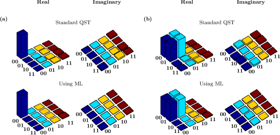
Figure 2.1: Real (left) and imaginary (right) parts of the experimental tomographs of the (a) $|00\rangle$ state, with a computed fidelity of 0.9937 using standard QST and a computed fidelity of 0.9992 using ML method for state estimation. (b) $\frac{1}{\sqrt{2}}(|00\rangle+|01\rangle)$ state, with a computed fidelity of 0.9928 using standard QST and a computed fidelity of 0.9991 using ML method for state estimation. The rows and columns are labeled in the computational basis ordered from $|00\rangle$ to $|11\rangle$.

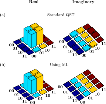
Figure 2.2: Real (left) and imaginary (right) parts of the experimental tomographs of the entangled state $\frac{1}{\sqrt{2}}(|01\rangle+|10\rangle)$ reconstructed (a) using standard QST and (b) using ML estimation. The fidelities computed using standard QST and using ML method for state estimation are 0.9933 and 0.9999 respectively. The rows and columns are labeled in the computational basis ordered from $|00\rangle$ to $|11\rangle$.

We performed state estimation of several different quantum states of two and three qubits, constructed on an NMR quantum information processor, using the ML estimation method. The results were compared every time with the results obtained by reconstruction using the standard QST protocol.

2.2.0.1 Fidelity measure and state estimation

The fidelity measures commonly used in NMR quantum computing are:

1. The fidelity measure $F_{1}$ is computed by measuring the overlap between theoretically expected and experimentally measured states [135]:

   $$F_{1}=\frac{Tr(\rho_{\rm theory}\rho_{\rm expt})}{\sqrt{(}Tr(\rho_{\rm theory}^{2}))\sqrt{(}Tr(\rho_{\rm expt}^{2}))}$$ (2.31)

2. The fidelity measure $F_{2}$ is computed by measuring the projection between the theoretically expected and experimentally measured states using the Uhlmann-Jozsa fidelity measure [136, 137]:

   $$F_{2}=\left(Tr\left(\sqrt{\sqrt{\rho_{\rm theory}}\rho_{\rm expt}\sqrt{\rho_{\rm theory}}}\right)\right)^{2}$$ (2.32)

where $\rho_{\rm theory}$ and $\rho_{\rm expt}$ denote the theoretically expected and experimentally reconstructed density matrices, respectively.

2.2.1 Comparison of separable states estimation

On a system of two qubits, we began by tomographing a pure state $|00\rangle$, as well as a superposition state $\frac{1}{\sqrt{2}}(|00\rangle+|01\rangle)$ (which can be written as a tensor product of the first qubit in the $|0\rangle$ state and the second qubit in a coherent superposition of the $|0\rangle$ and $|1\rangle$ states). The mean of ten to twenty-five experimentally determined data matrices were considered, and the reconstructed density matrices using the ML estimation method and using the standard QST method are shown as bar tomographs in Figure 2.1, with the states labeled in the computational basis in the order $|00\rangle$ to $|11\rangle$. Using standard QST, the reconstructed $|00\rangle$ state had negative eigenvalues: $\{0.994\pm 0.000,0.073\pm 0.006,-0.001\pm 0.002,-0.066\pm 0.005\}$, and state fidelity was computed with measure $F_{1}$ to be 0.9937 and with measure $F_{2}$ to be 0.9940. Reconstructing the state using ML estimation, we obtained all positive eigenvalues: $\{0.965\pm 0.001,0.035\pm 0.001,0.000\pm 0.000,0.000\pm 0.000\}$, while state fidelity was computed with measure $F_{1}$ to be 0.9992 and with measure $F_{2}$ to be 0.9652. For the superposition state $\frac{1}{\sqrt{2}}(|00\rangle+|01\rangle)$, state reconstruction using standard QST led to some negative eigenvalues: $\{1.011\pm 0.002,0.052\pm 0.005,0.016\pm 0.002,-0.079\pm 0.004\}$ with the fidelity measures $F_{1}$ and $F_{2}$ are 0.9928 and 1.0110 respectively. Using ML estimation on the other hand, led to all positive eigenvalues: $\{0.975\pm 0.001,0.025\pm 0.001,0.001\pm 0.000,0.000\pm 0.000\}$ with a state fidelity with measures $F_{1}$ and $F_{2}$ are 0.9991 and 0.9745. While state fidelities with $F_{1}$ measure are nearly the same (or slightly better when calculated after ML reconstruction of the density matrix), we find that by using the ML estimation method for state estimation, we always obtain a $\rho$ which is physically valid.

2.2.2 Comparison of entangled states estimation

It has been previously noted [119] that the standard QST protocol frequently leads to unphysical density matrices for entangled multiqubit states. Since entanglement has been posited to lie at the heart of quantum computational speedup, their construction and estimation is of prime importance. We used the ML estimation method to reconstruct two-qubit and three-qubit entangled states and evaluated the efficacy of this scheme to construct valid density matrices.

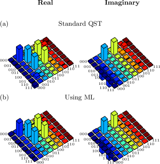
Figure 2.3: Real (left) and imaginary (right) parts of the experimental tomographs of the three-qubit maximally entangled state $|W\rangle=\frac{1}{\sqrt{3}}(i|001\rangle+|010\rangle+|100\rangle)$, reconstructed (a) using standard QST with a computed fidelity of 0.9833 and (b) using ML estimation with a computed fidelity of 0.9968. The rows and columns are labeled in the computational basis ordered from $|000\rangle$ to $|111\rangle$.

The state estimation of a two-qubit entangled Bell state $\frac{1}{\sqrt{2}}(|01\rangle+|10\rangle)$ is shown in Figure 2.2, using both QST and ML methods for density matrix reconstruction. Using the QST protocol for tomography, we obtain the eigenvalues: $\{0.996\pm 0.002,0.018\pm 0.001,0.005\pm 0.001,-0.019\pm 0.002\}$ with the first eigenvalue being negative, and with a computed fidelity with measure $F_{1}$ and $F_{2}$ are 0.9933 and 0.9964 respectively. Using ML method for state estimation leads to all positive eigenvalues: $\{0.993\pm 0.002,0.006\pm 0.001,0.001\pm 0.000,0.001\pm 0.000\}$ with a computed state fidelity with measures $F_{1}$ and $F_{2}$ are 0.9999 and 0.9926 respectively.

H

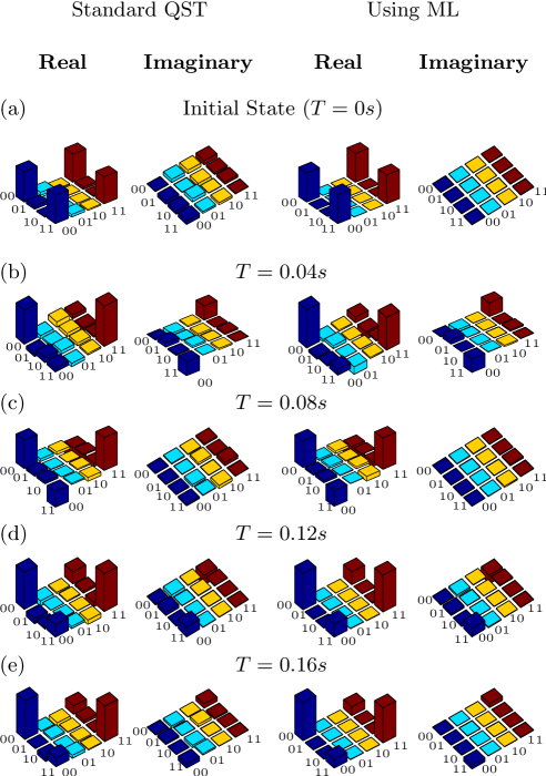
Figure 2.4: Real (left) and imaginary (right) parts of the experimental tomographs of the (a) $\frac{1}{\sqrt{2}}(|00\rangle+|11\rangle)$ state. Tomographs (b)-(e) depict the state at $T=0.04,0.08,0.12,0.16s$, with the tomographs on the left and the right representing the state estimated using standard QST and using ML estimation, respectively. The rows and columns are labeled in the computational basis ordered from $|00\rangle$ to $|11\rangle$.

Recently, schemes to construct maximally entangled three-qubit states from a generic state have been implemented on an NMR quantum information processor [138, 139]. We used these schemes to construct the maximally entangled $W$ state on a system of three qubits $|W\rangle=\frac{1}{\sqrt{3}}(i|001\rangle+|010\rangle+|100\rangle)$, and thereafter performed state estimation using both the standard QST and the ML methods. The experimentally reconstructed tomographs are depicted in Figure 2.3, with the states being labeled in the computational basis ordered from $|000\rangle$ to $|111\rangle$. After QST tomography on this three-qubit state, we obtained the eigenvalues: {0.939, 0.104, 0.078, 0.054, -0.002, -0.042, -0.061, -0.071}, and a calculated state fidelity $F_{1}$ is 0.9759 and $F_{2}$ is 0.9399. After performing state estimation using the ML method, the eigenvalues turned out to be all positive: {0.919, 0.036, 0.027, 0.008, 0.006, 0.002, 0.002, 0.000}, with a calculated state fidelity with $F_{1}$ is 0.9968 and with $F_{2}$ is 0.9191.

A topic of much research focus here is the accurate measurement of the decay of multiqubit entanglement with time. To study this, we performed state estimation of the entangled two-qubit state $\frac{1}{\sqrt{2}}(|00\rangle+|11\rangle)$ using both QST and ML protocols. The bar tomographs of the reconstructed density matrices at different times (T=0, 0.04, 0.08, 0.12, 0.16 sec) are shown in Figure 2.4.

The amount of entanglement that remains in the state after a certain time can be quantified by an entanglement parameter denoted by $\eta$ [63]. Since we are dealing with mixed bipartite states of two-qubit, all entangled states will be negative under partial transpose (NPT). For such NPT states, a reasonable measure of entanglement is the minimum eigenvalue of the partially transposed density operator. For a given experimentally tomographed density operator $\rho$, we obtain $\rho^{PT}$ by taking a partial transpose with respect to one of the qubits. The entanglement parameter $\eta$ for the state $\rho$ in terms of the smallest eigenvalue $E^{\rho}_{\rm Min}$ of $\rho^{PT}$ is defined as [63].

$$\eta=\left\{\begin{array}[]{ll}-E^{\rho}_{\rm Min}&{\rm if\leavevmode\nobreak\ }E^{\rho}_{\rm Min}<0\\ &\\ \phantom{-}0&{\rm if\leavevmode\nobreak\ }E^{\rho}_{\rm Min}>0\end{array}\right.$$ (2.33)

For the calculation of the entanglement parameter $\eta$, the purity factor $\epsilon\approx 1$, since, we are considering the subensemble of spins that have been prepared in the pseudopure state, and in which the spins are genuinely entangled as described in Chap. 1, Sec. 1.3.2.

A plot of the entanglement parameter $\eta$ with time is depicted in Figure 2.5, for the two-qubit maximally entangled Bell state $\frac{1}{\sqrt{2}}(|00\rangle+|11\rangle)$, estimated using both standard QST and the ML method. As can be seen from Figure 2.5, the QST method led to negative eigenvalues in the reconstructed (unphysical) density matrix and hence an overestimation of the entanglement parameter quantifying the residual entanglement in the state. The ML estimation method on the other hand, by virtue of its leading to a physical density matrix reconstruction every time, gives us a true measure of residual entanglement, and hence can be used to quantitatively study the decoherence of multiqubit entanglement. The difference between the two methods is statistically significant, as is evident from the graph, where the error bars are shown on each data point. The error is in fact very small, compared to the anomaly in the estimation of the entanglement.

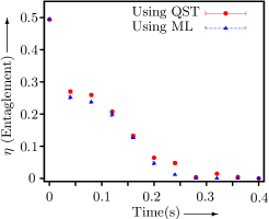
Figure 2.5: Plot of the entanglement parameter $\eta$ with time, using standard QST and ML protocols for state reconstruction, computed for the $\frac{1}{\sqrt{2}}(|00\rangle+|11\rangle)$ state.

2.3 Conclusions

We used the maximum likelihood estimation method for state estimation on an NMR quantum information processor, to circumvent the problem of unphysical density matrices that occur due to statistical errors while using the standard QST protocol. It has been previously shown that state reconstruction using QST, of entangled states and other fragile quantum states are particularly susceptible to errors, and can lead to unphysical density matrices for such states. We showed that the experimental density matrices reconstructed for entangled states of two and three qubits using the ML estimation method are always positive, definite and normalized. The state fidelities computed using fidelity measure $F_{1}$ are comparable for standard QST and using ML estimation. However if we use the fidelity measure $F_{2}$, the obtained state fidelity with ML estimation is less than the standard QST. The advantage of the ML estimation method is that it always leads to a valid density matrix and hence is a better estimator of the state of the quantum system. In the rest of this thesis we will use the ML estimation method for quantum state tomography and $F_{2}$ as the measure for state fidelity.

Chapter 3 Experimental protection of quantum states via a super-Zeno scheme

3.1 Introduction

Unwanted changes occur in quantum systems due to their interaction with the environment which leads to state degradation. This process, where quantum coherence is lost, is known as decoherence. Decoherence is a major obstacle in implementing quantum computing and quantum information processing schemes. In order to tackle this problem a number of techniques have been developed. The dynamical decoupling (DD) approach can be used to effectively decouple the system from its environment and thus decoherence can be suppressed [140, 141]. The idea that frequent measurements which project a quantum system back to its initial state can be used to not let the state evolve is known as the quantum Zeno effect [142, 143, 144, 145]. If the measurements project the system back into a finite-dimensional subspace that includes the initial state, the state evolution remains confined within this subspace and the subspace can be protected against leakage of population using a quantum Zeno strategy [146, 147]. Zeno-like schemes have been used for error prevention [148], and to enhance the entanglement of a state and bring it to a Bell state, even after entanglement sudden death [149, 150]. It has been shown that under certain assumptions, the Zeno effect can be realized with weak measurements and can protect an unknown encoded state against environmental effects [151]. All these strategies are based on our knowledge of the system-environment interaction and the state that needs to be preserved.

In a situation where the system state is known but there is no knowledge about its interaction with the environment, decoherence can be tackled by an interesting quantum Zeno-type strategy for state preservation. This is achieved by using a sequence of non-periodic short duration pulses and is called the super-Zeno scheme [60]. The super-Zeno scheme does not assume any Hamiltonian symmetry, does not involve projective quantum measurements and achieves a significant reduction of the leakage probability as compared to standard Zeno-based preservation schemes. The super-Zeno scheme for state protection is similar to universal dynamical decoupling schemes for multi-qubit states [61]. The only difference in the super-Zeno scheme is that non-periodic short duration between the unitary kicks are optimized numerically by minimizing the leakage probability. Similar schemes involving dynamical decoupling have been devised to suppress qubit pure dephasing and relaxation [152, 111]. Another scheme to preserve entanglement in a two-qubit spin-coupled system has been constructed, which unlike the super-Zeno scheme, is based on a sequence of operations performed periodically on the system in a given time interval [153].

There are several experimental implementations of the quantum Zeno phenomenon, including suppressing unitary evolution driven by external fields between the two states of a trapped ion [154], in atomic systems [155] and suppressing failure events in a linear optics quantum computing scheme [156]. Decoherence control in a superconducting qubit system has been proposed using the quantum Zeno effect [157]. Unlike the super-Zeno and dynamical decoupling schemes that are based on unitary pulses, the quantum Zeno effect achieves suppression of state evolution using projective measurements. The quantum Zeno effect was first demonstrated in NMR by a set of symmetric $\pi$ pulses [158], wherein pulsed magnetic field gradients and controlled-NOT gates were used to mimic projective measurements. The entanglement preservation of a Bell state in a two-spin system in the presence of anisotropy was demonstrated using a preservation procedure involving free evolution and unitary operations [28]. An NMR scheme to preserve a separable state was constructed using the super-Zeno scheme and the state preservation was found to be more efficient as compared to the standard Zeno scheme [62]. The quantum Zeno effect was used to stabilize superpositions of states of NMR qubits against dephasing, using an ancilla to perform the measurement [159]. Entanglement preservation based on a dynamic quantum Zeno effect was demonstrated using NMR wherein frequent measurements were implemented through entangling the target and measuring qubits [160].

In this chapter we demonstrate the use of the super-Zeno scheme, while the implementation of dynamical decoupling schemes will be taken up in later chapters of the thesis. Two applications of the super-Zeno scheme are described in this chapter: (i) Preservation of a state by freezing state evolution (one-dimensional subspace protection) and (ii) Subspace preservation by preventing leakage of population to an orthogonal subspace (two-dimensional subspace protection). Both kinds of protection schemes are experimentally demonstrated on separable as well as on maximally entangled two-qubit state. One-dimensional subspace protection is demonstrated on the separable $|11\rangle$ state and on the maximally entangled $\frac{1}{\sqrt{2}}(|01\rangle-|10\rangle)$ (singlet) state. Two-dimensional subspace preservation is demonstrated by choosing the $\{|01\rangle,|10\rangle\}$ subspace in the four-dimensional Hilbert space of two qubits, and implementing the super-Zeno subspace preservation protocol on three different states, namely $|01\rangle$, $|10\rangle$ and $\frac{1}{\sqrt{2}}(|01\rangle-|10\rangle)$ (singlet) states. Complete state tomography via maximally likelihood estimation as described in Chapter 2 is utilized to compute experimental density matrices at several time points. State fidelities at these time points were computed to evaluate how closely the states resemble the initially prepared states, with and without super-Zeno protection. The success of the super-Zeno scheme in protecting states in the two-dimensional subspace spanned by $\{|01\rangle,|10\rangle\}$ is evaluated by computing a leakage parameter, which computes leakage to the orthogonal subspace spanned by $\{|00\rangle,|11\rangle\}$. For entangled states, an additional entanglement parameter is constructed to quantify the residual entanglement in the state over time. State fidelities, the leakage parameter and the entanglement parameter are plotted as a function of time, to quantify the performance of the super-Zeno scheme.

3.2 The super-Zeno scheme

The super-Zeno algorithm to preserve quantum states has been developed along lines similar to bang-bang control schemes, and limits the quantum system’s evolution to a desired subspace using a series of unitary kicks [60]. A finite-dimensional Hilbert space $\cal{H}$ can be written as a direct sum of two orthogonal subspaces $\cal{P}$ and $\cal{Q}$. The super-Zeno scheme involves a unitary kick J, which can be constructed as

$${\bf J=Q-P}$$ (3.1)

where $\bf P,Q$ are the projection operators onto the subspaces $\cal{P},\cal{Q}$ respectively. The action of this specially crafted pulse ${\bf J}$ on a state $|\psi\rangle\in\cal{H}$ is as follows:

$${\bf J}|\psi\rangle = -|\psi\rangle,\quad|\psi\rangle\in{\cal P}$$

$${\bf J}|\psi\rangle = |\psi\rangle,\quad|\psi\rangle\in{\cal Q}$$ (3.2)

where ${\cal P}$ is the subspace being preserved [60].

The basic aim of this scheme is to design a sequence of appropriately spaced inverting pulses, such that if the system is initially in a state $|\psi\rangle\in{\cal P}$, then the leakage of the system state over time to ${\cal Q}$ after this pulse sequence is minimum. The inverting pulse J produces destructive interference of quantum amplitudes and reduces the transition rate from the $\cal{P}$ subspace to $\cal{Q}$. Let the system be prepared in a general state $|\psi(0)\rangle=|p\rangle\in\cal{P}$, the system Hamiltonian $\mathbf{H}$ is bounded and the unitary operator corresponding to the evolution for a time interval $t$ is given by

$$\mathbf{U(t)=e^{{-\iota Ht}/{\hbar}}}.$$ (3.3)

For simplicity we use natural units and $\hbar=1$. Then, the state $|\psi(0)\rangle$ after time $t$ is

$$\mathbf{|\psi(t)\rangle=e^{-\iota\mathbf{H}t}|\psi(0)\rangle}$$ (3.4)

The amplitude of the system to be in a state $\mathbf{|q\rangle}\in\cal{Q}$ after a time interval $t$ is given by

$$\mathbf{\langle q|e^{-\iota\mathbf{H}t}|\psi(0)\rangle}$$ (3.5)

However, if we evolve the system for the half interval t/2, subject the system to an inverting pulse J, and then further evolve by a time t/2, the above amplitude turns out to be

$$\mathbf{\langle q|e^{-\iota\mathbf{H}t/2}\mathbf{J}e^{-\iota\mathbf{H}t/2}|\psi(0)\rangle}$$ (3.6)

For a small time interval t and the unitary operator $\mathbf{U(t)}$ satisfying $\mathbf{U(t)=\textbf{I}+\mathcal{O}(t)}$

$$\mathbf{\langle q|\left(I+\frac{-\iota\mathbf{H}t}{2}\right)\mathbf{J}\left(I+\frac{-\iota\mathbf{H}t}{2}\right)|\psi(0)\rangle}$$ (3.7)

$$\mathbf{=\langle q|\mathbf{J}|p\rangle+\langle q|\mathbf{J}\frac{-\iota\mathbf{H}t}{2}+\frac{-\iota\mathbf{H}t}{2}\mathbf{J}|p\rangle+\mathcal{O}(t^{2})}$$

$$\mathbf{=\langle q|\mathbf{J}\frac{-\iota\mathbf{H}t}{2}|p\rangle+\langle q|\frac{-\iota\mathbf{H}t}{2}\mathbf{J}|p\rangle+\mathcal{O}(t^{2})}$$

$$\mathbf{=\langle q|\frac{-\iota\mathbf{H}t}{2}|p\rangle-\langle q|\frac{-\iota\mathbf{H}t}{2}|p\rangle+\mathcal{O}(t^{2})}$$

Due to the action of $\mathbf{J}$, destructive interference takes place between the two amplitudes of $\mathcal{O}(t)$ in Eq.(3.7) and we are left with terms of $\mathcal{O}(t^{2})$ term and higher, which are negligible for a small time interval $t$. In general, if the matrix elements of $\mathbf{U(t)}$ i.e $\mathbf{U_{qp}}$ and $\mathbf{U_{pq}}$ are of $\mathcal{O}(t^{(r)})$ then the transition amplitude

$$\mathbf{\langle q|U(t).J.U(t)|p\rangle=-\sum_{p^{\prime}\in\cal{P}}U_{qp^{\prime}}U_{p^{\prime}p}+\sum_{q^{\prime}\in\cal{Q}}U_{qq^{\prime}}U_{q^{\prime}p}-U_{qp}U_{pp}-U_{qq}U_{qp}}$$

$$\mathbf{=\mathcal{O}(t^{r+1})-U_{qp}U_{pp}-U_{qq}U_{qp}=\mathcal{O}(t^{r+1})}$$ (3.8)

where a precise cancellation of the amplitude of $\mathbf{\mathcal{O}(t^{r})}$ term occurs [60].

It is important to note that $\mathbf{V(t)=U(t).J.U(t)}$ tends to $\mathbf{J}$ as $t\rightarrow 0$ but $\mathbf{V(t)^{2}}$ tends to $\mathbf{I}$ and if $\mathbf{V(t)=J+\mathcal{O}(t)}$ and $\mathbf{V(t)_{qp}=\mathcal{O}(t^{r})}$

$$\mathbf{\langle q|V(t)^{2}|p\rangle} = \mathbf{-\sum_{p^{\prime\prime}\in\cal{P}}V(t)_{qp^{\prime}}V(t)_{p^{\prime}p}+\sum_{q^{\prime}\in\cal{Q}}V(t)_{qq^{\prime}}V(t)_{q^{\prime}p}}$$

$$\mathbf{-V(t)_{qp}V(t)_{pp}-V(t)_{qq}V(t)_{qp}}$$

$$= \mathbf{\mathcal{O}(t^{r+1})+V(t)_{qp}(V(t)_{qq}+V(t)_{pp})}$$

$$\mathbf{\langle q|V(t)^{2}|p\rangle=\mathcal{O}(t^{r+1})}$$ (3.9)

Hence, if for $\mathbf{U_{0}(t)}$ the transition amplitude to an orthogonal state is proportional to $t$, then for the operator $\mathbf{U_{1}(t)=U_{0}(t).J.U_{0}(t)}$ from Eq. (3.8), the transition amplitude is $\mathcal{O}(t^{2})$. For $\mathbf{U_{1}^{2}}$ using Eq. (3.2), the transition amplitude is $\mathcal{O}(t^{3})$ [60]. Using this result, it is straight forward to construct a pulse sequence where the transition amplitude is $\mathcal{O}(t^{r})$ for any positive integer $r$ by recursion. Defining operators $\mathbf{U}_{m}$ by the recursion relations

$${\bf U}_{m+1}(t) = {\bf U}_{m}(t/2)\leavevmode\nobreak\ {\mathbf{J}}\leavevmode\nobreak\ {\bf U}_{m}(t/2),{\rm\leavevmode\nobreak\ for\leavevmode\nobreak\ }m{\rm\leavevmode\nobreak\ even}$$ (3.10)

$$= {\bf U}_{m}(t/2)\leavevmode\nobreak\ {\bf U}_{m}(t/2),{\rm\leavevmode\nobreak\ for}\leavevmode\nobreak\ m{\rm\leavevmode\nobreak\ odd}$$

with ${\bf U}_{0}={\bf U}_{0}(t)$. Then, by induction, it follows that the transition amplitude $\langle q|{\bf U}_{m}|p\rangle$ is of order ${\mathcal{O}}(t^{m+1})$.

$\mathbf{U}_{m}(t)$ can be written explicitly as a product of $\mathbf{U}_{0}(t/2^{m})$’s and $\mathbf{J}$’s. For example

$$\mathbf{U}_{1}(t) = \mathbf{U}_{0}(t/2){\mathbf{J}}\mathbf{U}_{0}(t/2),$$

$$\mathbf{U}_{2}(t) = [\mathbf{U}_{0}(t/4){\mathbf{J}}\mathbf{U}_{0}(t/4)]^{2},$$

$$\mathbf{U}_{3}(t) = [\mathbf{U}_{0}(t/8){\mathbf{J}}\mathbf{U}_{0}(t/8)]^{2}{\mathbf{J}}[\mathbf{U}_{0}(t/8){\mathbf{J}}\mathbf{U}_{0}(t/8)]^{2}.$$ (3.11)

If $N_{m}$ are the number of pulses used in the sequence ${\mathbf{U}}_{m}$, then it is easily verified that

$$N_{m}=(2^{m+1}-2)/3,{\rm\leavevmode\nobreak\ for}\leavevmode\nobreak\ m{\rm\leavevmode\nobreak\ even},$$

$$=(2^{m+1}-1)/3,{\rm\leavevmode\nobreak\ for}\leavevmode\nobreak\ m{\rm\leavevmode\nobreak\ odd}.$$ (3.12)

The leakage probability $L_{m}$ from subspace $\mathcal{P}$ to subspace $\mathcal{Q}$ for operator $\mathbf{U}_{m}$ applied for a total time $T$ is

$$L_{m}=\sum_{q\in Q}|\langle q|\mathbf{U}_{m}|p\rangle|^{2}\leq 2^{-m(m+1)}[ET]^{2m+2}$$ (3.13)

where $E=|\mathbf{H}|$ is the norm of the Hamiltonian as defined by

$$|\mathbf{H}|={\genfrac{}{}{0.0pt}{}{\mathrm{sup}}{\psi}}\ ||\mathbf{H}|\psi\rangle||\leavevmode\nobreak\ /\leavevmode\nobreak\ ||\leavevmode\nobreak\ |\psi\rangle||$$ (3.14)

where the $\mathrm{sup}$ notation is defined as (for any function $f$ and constraint set ${\cal X}$)

$$\genfrac{}{}{0.0pt}{}{\mathrm{sup}}{x\in{\cal X}}\ f(x)\geq f(v)\ \ \forall\ \ v\ \in\ {\cal X}$$ (3.15)

The total number of inverting pulses $N_{m}$ required to keep the leakage probability less than $\epsilon$ up to time $T$ grows as $\frac{2}{3}ET$ $2^{{log_{2}(E^{2}T^{2}/\epsilon)}^{1/2}}$ [60]. It is possible to decrease the required number of pulses significantly by allowing the intervals between the inverting pulses to be varied continuously independent of each other.

For a given $N$, further improvements are possible and one can express $\langle q|{W}_{N}(t)|p\rangle$ as a Taylor series in powers of $t$. The coefficients of different powers of $t$ are sums of matrix-elements of the type $\langle q|{\bf H}^{n_{1}}{\mathbf{J}}{\bf H}^{n_{2}}{\mathbf{J}}..|p\rangle$, with coefficients that are polynomials of $\{x_{j}\}$. Thus, the total super-Zeno sequence for $N$ pulses is given by

$$W_{N}(t)=U(x_{N+1}t){\bf J}\dots\bf JU(x_{2}t){\bf J}U(x_{1}t)$$ (3.16)

where $U$ denotes unitary evolution under the system Hamiltonian and $x_{i}t$ is the time interval between the $i$th and $(i+1)$th pulse. The sequence $\{x_{i}t\}$ of time intervals between pulses is optimized such that if the system starts out in the subspace $\cal P$, after measurement the probability of finding the system in the orthogonal subspace $\cal Q$ is minimized. In this work we used four inverting pulses interspersed with five unequal time intervals in each repetition of the preserving super-Zeno sequence. The optimized sequence is given by $\{x_{i}\}=\{\beta,1/4,1/2-2\beta,1/4,\beta\}$ with $\beta=(3-\sqrt{5})/8,i=1\dots 5$ and $t$ is a fixed time interval (we used the $x_{i}$ as worked out in Ref. [60]).

The explicit form of the unitary kick ${\bf J}$ depends on the subspace that needs to be preserved, and in the following section, we implement several illustrative examples for both separable and entangled states embedded in one- and two-dimensional subspaces of two qubits.

3.3 Experimental implementations of super-Zeno scheme

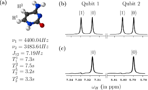
Figure 3.1: (a) Molecular structure of cytosine with the two qubits labeled as $H^{1}$ and $H^{2}$ and tabulated system parameters with chemical shifts $\nu_{i}$ and scalar coupling $J_{12}$ (in Hz) and relaxation times $T_{1}$ and $T_{2}$ (in seconds) (b) NMR spectrum obtained after a $\pi/2$ readout pulse on the thermal equilibrium state. The resonance lines of each qubit are labeled by the corresponding logical states of the other qubit and (c) NMR spectrum of the pseudopure $|00\rangle$ state.

3.3.1 NMR system details

The two protons of the molecule cytosine encode the two qubits. The two-qubit molecular structure, system parameters and NMR spectra of the pseudopure and thermal initial states are shown in Figs. 3.1(a)-(c). The Hamiltonian of a two-qubit system in the rotating frame is given by

$$H=-(\omega_{1}-\omega_{rf})I_{1z}-(\omega_{2}-\omega_{rf})I_{2z}+2\pi J_{12}I_{1z}I_{2z}$$ (3.17)

where $\omega_{i}=2\pi\nu_{i}$ are the chemical shift of the spins in rad s^-1, $\omega_{{\rm rf}}$ reference chemical shift of rotating frame, and $J_{12}$ is the spin-spin coupling constant. An average longitudinal T₁ relaxation time of 7.4 s and an average transverse T₂ relaxation time of 3.25 s was experimentally measured for both the qubits. The experiments were performed at an ambient temperature of 298 K on a Bruker Avance III 600 MHz NMR spectrometer equipped with a QXI probe. The two-qubit system was initialized into the pseudopure state $|00\rangle$ using the spatial averaging technique [24], with the density operator given by

$$\rho_{00}=\frac{1-\epsilon}{4}I+\epsilon|00\rangle\langle 00|$$ (3.18)

with a thermal polarization $\epsilon\approx 10^{-5}$ and $I$ being a $4\times 4$ identity operator. The experimentally created pseudopure state $|00\rangle$ was tomographed with a fidelity of $0.99$. The pulse propagators for selective excitation were constructed using the GRAPE algorithm [25] to design the amplitude and phase modulated rf profiles. Selective excitation was typically achieved with pulses of duration 1 ms. Numerically generated GRAPE pulse profiles were optimized to be robust against rf inhomogeneity and had an average fidelity of $\geq 0.99$. All experimental density matrices were reconstructed using a quantum state tomography via maximum likelihood protocol (Chapter 2). The fidelity of an experimental density matrix was computed using Eq. (2.32).

3.3.2 Super-Zeno scheme for state preservation

When the subspace $\cal P$ is a one-dimensional subspace, and hence consists of a single state, the super-Zeno scheme becomes a state preservation scheme.

3.3.2.1 Preservation of product states:

We begin by implementing the super-Zeno scheme on the product state $|11\rangle$ of two qubits, where the Hilbert space can be decomposed as a direct sum of the subspaces ${\cal P}=\{|11\rangle\}$ and ${\cal Q}=\{|00\rangle,|01\rangle,|10\rangle)\}$. The super-Zeno pulse $\bf J$ to protect the state $|11\rangle\in{\cal P}$ is given by Eqn. (3.1):

$${\bf J}=I-2|11\rangle\langle 11|$$ (3.19)

with the corresponding matrix form

$${\bf J}=\left(\begin{array}[]{cccc}1&0&0&0\\ 0&1&0&0\\ 0&0&1&0\\ 0&0&0&-1\end{array}\right)$$ (3.20)

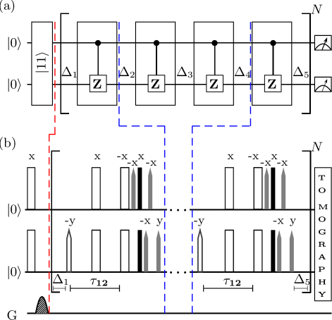
Figure 3.2: (a) Quantum circuit for preservation of the state $|11\rangle$ using the super-Zeno scheme. $\Delta_{i}=x_{i}t,(i=1...5)$ denote time intervals punctuating the unitary operation blocks. Each unitary operation block contains a controlled-phase gate ($Z$), with the first (top) qubit as the control and the second (bottom) qubit as the target. The entire scheme is repeated $N$ times before measurement (for our experiments $N=30$). (b) Block-wise depiction of the corresponding NMR pulse sequence. A $z$-gradient is applied just before the super-Zeno pulses, to clean up undesired residual magnetization. The unfilled and black rectangles represent hard $180^{0}$ and $90^{0}$ pulses respectively, while the unfilled and gray-shaded conical shapes represent $180^{0}$ and $90^{0}$ pulses (numerically optimized using GRAPE) respectively; $\tau_{12}$ is the evolution period under the $J_{12}$ coupling. Pulses are labeled with their respective phases and unless explicitly labeled, the phase of the pulses on the second (bottom) qubit are the same as those on the first (top) qubit.

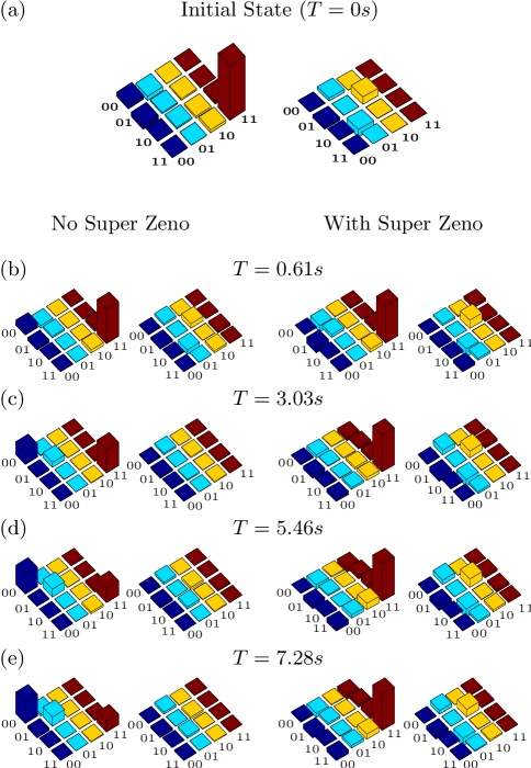
Figure 3.3: Real (left) and imaginary (right) parts of the experimental tomographs of the (a) $|11\rangle$ state, with a computed fidelity of 0.99. (b)-(e) depict the state at $T=0.61,3.03,5.46,7.28$ s, with the tomographs on the left and the right representing the state without and after applying the super-Zeno preserving scheme, respectively. The rows and columns are labeled in the computational basis ordered from $|00\rangle$ to $|11\rangle$.

The super-Zeno circuit to preserve the $|11\rangle$ state, and the corresponding NMR pulse sequence is given in Fig. 3.2. The controlled-phase gate ($Z$) in Fig. 3.2(a) which replicates the unitary kick ${\bf J}$ for preservation of the $|11\rangle$ state is implemented using a set of three sequential gates: two Hadamard gates on the second qubit sandwiching a controlled-NOT gate (CNOT₁₂), with the first qubit as the control and the second qubit as the target. The $\Delta_{i}$ time interval in Fig. 3.2(a) is given by $\Delta_{i}=x_{i}t$, with $x_{i}$ as defined in Eq. (3.16). The five $\Delta_{i}$ time intervals were worked to be $0.095$ ms, $0.25$ ms, $0.3$ ms, $0.25$ ms, and $0.095$ ms respectively, for $t=1$ ms. One run of the super-Zeno circuit (with four inverting ${\bf J}$s and five $\Delta_{i}$ time evolution periods) takes approximately $300$ ms and the entire preserving sequence $W_{N}(t)$ in Eq. (3.16) was applied $30$ times. The final state of the system was reconstructed using state tomography and the real and imaginary parts of the tomographed experimental density matrices without any preservation and after applying the super-Zeno scheme, are shown in Fig. 3.3. The initial $|11\rangle$ state (at time $T=0$ s) was created (using the spatial averaging scheme) with a fidelity of 0.99. The tomographs (on the right in Fig. 3.3) clearly show that state evolution has been frozen with the super-Zeno scheme.

3.3.2.2 Preservation of entangled states

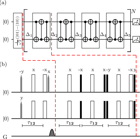
Figure 3.4: (a) Quantum circuit for preservation of the singlet state using the super-Zeno scheme. $\Delta_{i},(i=1...5)$ denote time intervals punctuating the unitary operation blocks. The entire scheme is repeated $N$ times before measurement (for our experiments $N=10$). (b) NMR pulse sequence corresponding to one unitary block of the circuit in (a). A $z$-gradient is applied just before the super-Zeno pulses, to clean up undesired residual magnetization. The unfilled rectangles represent hard $180^{0}$ pulses, the black filled rectangles representing hard $90^{0}$ pulses, while the shaded shapes represent numerically optimized (using GRAPE) pulses and the gray-shaded shapes representing $90^{0}$ pulses respectively; $\tau_{12}$ is the evolution period under the $J_{12}$ coupling. Pulses are labeled with their respective phases and unless explicitly labeled, the phase of the pulses on the second (bottom) qubit are the same as those on the first (top) qubit.

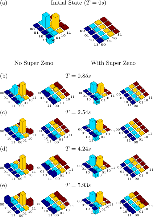
Figure 3.5: Real (left) and imaginary (right) parts of the experimental tomographs of the (a) $\frac{1}{\sqrt{2}}(|01\rangle-|10\rangle)$ (singlet) state, with a computed fidelity of 0.99. (b)-(e) depict the state at $T=0.85,2.54,4.24,5.93$ s, with the tomographs on the left and the right representing the state without and after applying the super-Zeno preserving scheme, respectively. The rows and columns are labeled in the computational basis ordered from $|00\rangle$ to $|11\rangle$.

We next apply the super-Zeno scheme to preserve an entangled state in our system of two qubits. We chose the singlet state $\frac{1}{\sqrt{2}}(|01\rangle-|10\rangle)$ as the entangled state to be preserved. It is well known that entanglement is an important but fragile resource for quantum information processing and constructing schemes to protect entangled states from evolving into other states, is of considerable interest in quantum information processing  [1].

We again write the Hilbert space as a direct sum of two subspaces: the subspace being protected and the subspace orthogonal to it. In this case, the one-dimensional subspace ${\cal P}$ being protected is

$${\cal P}=\left\{\frac{1}{\sqrt{2}}\left(|01\rangle-|10\rangle\right)\right\}$$ (3.21)

and the orthogonal subspace ${\cal Q}$ into which one would like to prevent leakage is

$${\cal Q}=\left\{\frac{1}{\sqrt{2}}(|01\rangle+|10\rangle),|00\rangle,|11\rangle\right\}$$ (3.22)

The super-Zeno pulse to protect the singlet state as constructed using Eq. (3.1) is:

$${\bf J}=I-\left(|01\rangle\langle 01|+|10\rangle\langle 10|-|01\rangle\langle 10|-|10\rangle\langle 01|\right)$$ (3.23)

with the corresponding matrix form:

$${\bf J}=\left(\begin{array}[]{cccc}1&0&0&0\\ 0&0&1&0\\ 0&1&0&0\\ 0&0&0&1\end{array}\right)$$ (3.24)

The quantum circuit and the NMR pulse sequence for preservation of the singlet state using the super-Zeno scheme are given in Fig. 3.4. Each J inverting pulse in the unitary block in the circuit is decomposed as a sequential operation of three non-commuting controlled-NOT gates: CNOT₁₂-CNOT₂₁-CNOT₁₂, where CNOT_ij denotes a controlled-NOT with $i$ as the control and $j$ as the target qubit. The five $\Delta_{i}$ time intervals were worked to be $0.95$ ms, $2.5$ ms, $3$ ms, $2.5$ ms, and $0.95$ ms respectively, for $t=10$ ms. One run of the super-Zeno circuit (with four inverting ${\bf J}$s and five $\Delta_{i}$ time evolution periods) takes approximately $847$ ms and the entire super-Zeno preserving sequence $W_{N}(t)$ in Eq. (3.16), is applied $10$ times.

The singlet state was prepared from an initial pseudopure state $|00\rangle$ by a sequence of three gates: a non-selective NOT gate (hard $\pi_{x}$ pulse) on both qubits, a Hadamard gate and a CNOT₁₂ gate. The singlet state thus prepared was computed to have a fidelity of 0.99. The effect of chemical shift evolution during the delays was compensated for with refocusing pulses. The final singlet state has been reconstructed using state tomography, and the real and imaginary parts of the tomographed experimental density matrices without any preservation and after applying the super-Zeno scheme, are shown in Fig. 3.5. As can be seen from the experimental tomographs in Fig. 3.5, the evolution of the singlet state is almost completely frozen by the super-Zeno sequence upto nearly 6 s, while without any preservation the state has leaked into the orthogonal subspace within 2 s.

Figure 3.6: Plot of fidelity versus time of (a) the $|11\rangle$ state and (b) the $\frac{1}{\sqrt{2}}(|01\rangle-|10\rangle)$ (singlet) state, without any preserving scheme and after the super-Zeno preserving sequence. The fidelity of the state with the super-Zeno preservation remains close to 1.

3.3.2.3 Estimation of state fidelity

The plots of state fidelity versus time are shown in Fig. 3.6 for the state $|11\rangle$ and the singlet state, with and without the super-Zeno preserving sequence. The signal attenuation has been ignored and the deviation density matrix is renormalized at every point and the state fidelity is estimated using the definition in Eq. (2.32). Renormalization is performed since our focus here is on the quantum state of the spins contributing to the signal and not on the number per se of participating spins [161]. The norm of deviation density matrix is proportional to the intensity of the tomographed spectra and is proportional to the number of spins contributing to the signal intensity. Due to super-Zeno preserving pulses, an attenuation in signal intensity takes place and we renormalize the intensity of the of the tomographed spectra in order to compensate for this attenuation. The plot of signal intensity versus time is shown in Fig. 3.7 for the state $|11\rangle$ and the singlet state, with the super-Zeno preserving sequence. The exponential intensity decay constant is $0.136\pm 0.006$ s^-1 for the $|11\rangle$ state and $0.393\pm 0.013$ s^-1 for the singlet state.

The plots in Fig. 3.6 and the tomographs in Fig. 3.3 and Fig. 3.5 show that with super-Zeno protection, the state remains confined to the $|11\rangle$ (singlet) part of the density matrix, while without the protection scheme, the state leaks into the orthogonal subspace. As seen from both plots in Fig. 3.6, the state evolution of specific states can be arrested for quite a long time using the super-Zeno preservation scheme, while leakage probability of the state to other states in the orthogonal subspace spanned by ${\cal Q}$ is minimized. A similar renormalization procedure is adopted in the subsequent sections where we plot the leak fraction and entanglement parameters (Fig. 3.12 and Fig. 3.13).

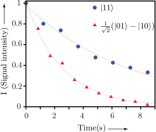
Figure 3.7: Plot of signal intensity versus time of the $|11\rangle$ state and the $\frac{1}{\sqrt{2}}(|01\rangle-|10\rangle)$ (singlet) state, after the super-Zeno preserving sequence.

3.3.3 Super-Zeno for subspace preservation

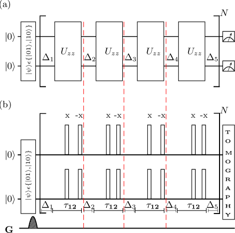
Figure 3.8: (a) Quantum circuit for preservation of the $\{01,10\}$ subspace using the super-Zeno scheme. $\Delta_{i},(i=1...5)$ denote time intervals punctuating the unitary operation blocks. The entire scheme is repeated $N$ times before measurement (for our experiments $N=30$). (b) NMR pulse sequence corresponding to the circuit in (a). A $z$-gradient is applied just before the super-Zeno pulses, to clean up undesired residual magnetization. The unfilled rectangles represent hard $180^{0}$ pulses; $\tau_{12}$ is the evolution period under the $J_{12}$ coupling. Pulses are labeled with their respective phases.

While in the previous subsection, the super-Zeno scheme was shown to be effective in arresting the evolution of a one-dimensional subspace (as applied to the cases of a product and an entangled state), the scheme is in fact more general. For example, if we choose a two-dimensional subspace in the state space of two qubits and protect it by the super-Zeno scheme, then any state in this subspace is expected to remain within this subspace and not leak into the orthogonal subspace. While the state can meander within this subspace, its evolution out of the subspace is frozen.

We now turn to implementing the super-Zeno scheme for subspace preservation, by constructing the J operator to preserve a general state embedded in a two-dimensional subspace. We choose the subspace spanned by ${\cal P}=\{|01\rangle,|10\rangle\}$ as the subspace to be preserved, with its orthogonal subspace now being ${\cal Q}=\{|00\rangle,|11\rangle\}$. It is worth noting that within the subspace being protected, we have product as well as entangled states.

The super-Zeno pulse J to protect a general state $|\psi\rangle\in P$ can be constructed as:

$${\bf J}=I-2\left(|01\rangle\langle 01|+|10\rangle\langle 10|\right)$$ (3.25)

with the corresponding matrix form

$${\bf J}=\left(\begin{array}[]{cccc}1&0&0&0\\ 0&-1&0&0\\ 0&0&-1&0\\ 0&0&0&1\end{array}\right)$$ (3.26)

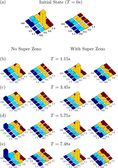
Figure 3.9: Real (left) and imaginary (right) parts of the experimental tomographs of the (a) $|10\rangle$ state in the two-dimensional subspace $\{01,10\}$, with a computed fidelity of 0.98. (b)-(e) depict the state at $T=1.15,3.45,5.75,7.48$ s, with the tomographs on the left and the right representing the state without and after applying the super-Zeno preserving scheme, respectively. The rows and columns are labeled in the computational basis ordered from $|00\rangle$ to $|11\rangle$.

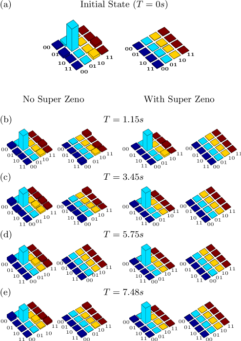
Figure 3.10: Real (left) and imaginary (right) parts of the experimental tomographs of the (a) $|01\rangle$ state in the two-dimensional subspace $\{01,10\}$, with a computed fidelity of 0.99. (b)-(e) depict the state at $T=1.15,3.45,5.75,7.48$ s, with the tomographs on the left and the right representing the state without and after applying the super-Zeno preserving scheme, respectively. The rows and columns are labeled in the computational basis ordered from $|00\rangle$ to $|11\rangle$.

The quantum circuit and corresponding NMR pulse sequence to preserve a general state in the $\{|01\rangle,|10\rangle\}$ subspace is given in Fig. 3.8. The unitary kick (denoted as $U_{zz}$ in the unitary operation block in Fig. 3.8(a)) is implemented by tailoring the gate time to the $J$-coupling evolution interval of the system Hamiltonian, sandwiched by non-selective $\pi$ pulses (NOT gates), to refocus undesired chemical shift evolution during the action of the gate. The five $\Delta_{i}$ intervals were worked to be $0.95$ ms, $2.5$ ms, $3$ ms, $2.5$ ms and $0.95$ ms respectively, for $t=10$ ms. One run of the super-Zeno circuit (with four inverting ${\bf J}$s and five $\Delta_{i}$ time evolution periods) takes approximately $288$ ms and the entire super-Zeno preserving sequence $W_{N}(t)$ in Eqn. (3.16), is applied $30$ times.

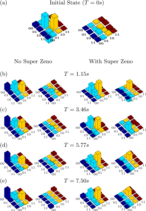
Figure 3.11: Real (left) and imaginary (right) parts of the experimental tomographs of the (a) $\frac{1}{\sqrt{2}}(|01\rangle-|10\rangle)$ (singlet) state in the two-dimensional subspace $\{01,10\}$, with a computed fidelity of 0.98. (b)-(e) depict the state at $T=1.15,3.46,5.77,7.50$ s, with the tomographs on the left and the right representing the state without and after applying the super-Zeno preserving scheme, respectively. The rows and columns are labeled in the computational basis ordered from $|00\rangle$ to $|11\rangle$.

3.3.3.1 Preservation of product states in the subspace

We implemented the subspace-preserving scheme on two different (separable) states $|01\rangle$ and $|10\rangle$ in the subspace ${\cal P}$. The efficacy of the preserving unitary is verified by tomographing the experimental density matrices at different time points and computing the state fidelity. Both the $|01\rangle$ and $|10\rangle$ states remain within the subspace ${\cal P}$ and do not leak out to the orthogonal subspace ${\cal Q}=\{|00\rangle,|11\rangle\}$.

The final $|10\rangle$ state has been reconstructed using state tomography, and the real and imaginary parts of the experimental density matrices without any preservation and after applying the super-Zeno scheme, tomographed at different time points, are shown in Fig. 3.9. As can be seen from the experimental tomographs, the evolution of the $|10\rangle$ state out of the subspace is almost completely frozen by the super-Zeno sequence upto nearly 7.5 s, while without any preservation the state has leaked into the orthogonal subspace within 3.5 s. The tomographs showed in Fig. 3.10 for the $|01\rangle$ state, show a similar level of preservation.

3.3.3.2 Preservation of an entangled state in the subspace

We now prepare an entangled state (the singlet state) embedded in the two-dimensional ${\cal P}=\{|01\rangle,|10\rangle\}$ subspace, and used the subspace-preserving scheme described in Fig. 3.8 to protect ${\cal P}$. The singlet state was reconstructed using state tomography, and the real and imaginary parts of the tomographed experimental density matrices without any preservation and after applying the super-Zeno scheme, are shown in Fig. 3.11. As can be seen from the experimental tomographs, the state evolution remains within the ${\cal P}$ subspace but the state itself does not remain maximally entangled.

Figure 3.12: Plot of leakage fraction from the $\{|01\rangle,|10\rangle\}$ subspace to its orthogonal subspace $\{|00\rangle,|11\rangle\}$ of (a) the $|10\rangle$ state and (b) the $\frac{1}{\sqrt{2}}(|01\rangle-|10\rangle)$ (singlet) state, without any preservation and after applying the super-Zeno sequence. The leakage to the orthogonal subspace is minimal (remains close to zero) after applying the super-Zeno scheme.

3.3.3.3 Estimating leakage outside subspace

An ensemble of spins initially prepared in a state belonging to the subspace ${\cal P}=\{|01\rangle,|10\rangle\}$, can evolve to the orthogonal subspace ${\cal Q}=\{|00\rangle,|11\rangle\}$ due to unwanted interactions with its environment. This evolution of the state to the orthogonal subspace is called leakage. We applied super-Zeno scheme to protect leakage of a state from subspace $\cal{P}$ to subspace $\cal{Q}$. The subspace-preserving capability of the circuit given in Fig. 3.8 was quantified by computing a leakage parameter that defines the amount of leakage of the state to the orthogonal ${\cal Q}=\{|00\rangle,|11\rangle\}$ subspace.

For a given density operator $\rho$ the “leak (fraction)” $\delta$, into the subspace ${\cal Q}$ is defined as

$$\delta=\langle 00|\rho|00\rangle+\langle 11|\rho|11\rangle$$ (3.27)

The leak (fraction) $\delta$ represents the number of spins of the ensemble that have migrated to the subspace $\cal{Q}$ divided by the total number of spins in the ensemble; $\delta$ is equal to one when all the states remain in the subspace $\cal{P}$ and is equal to zero if all the states have leaked to the subspace $\cal{Q}$. The leak (fraction) $\delta$ versus time is plotted in Figs. 3.12(a) and (b), for the $|10\rangle$ and the singlet state respectively, with and without applying the super-Zeno subspace-preserving sequence. The leakage parameter remains close to zero for both kinds of states, proving the success and the generality of the super-Zeno scheme.

3.3.4 Preservation of entanglement

The amount of entanglement that remains in the state after a certain time is quantified by an entanglement parameter denoted by $\eta$ as described in Chap. 2, Sec. 2.2.2. We will use this entanglement parameter $\eta$ to quantify the amount of entanglement at different times. The maximally entangled singlet state was created and its evolution studied in two different scenarios. In the first scenario described in Sec. 3.3.2, the singlet state was protected against evolution by the application of the super-Zeno scheme. In the second scenario described in Sec. 3.3.3, a two-dimensional subspace containing the singlet state was protected using the super-Zeno scheme. For the former case, one expects that the state will remain a singlet state, while in the latter case, it can evolve within the protected two-dimensional subspace. Since in the second case, the protected subspace contains entangled as well as separable states, one does not expect preservation of entanglement to the same extent as expected in the first case, where the one-dimensional subspace defined by the singlet state itself is protected. The experimental tomographs at different times and fidelity for the case of state protection and the leakage fraction for the case of subspace protection have been discussed in detail in the previous subsections.

Figure 3.13: Plot of entanglement parameter $\eta$ with time, with and without applying the super-Zeno sequence, computed for (a) the $\frac{1}{\sqrt{2}}(|01\rangle-|10\rangle)$ (singlet) state, and (b) the same singlet state when embedded in the subspace $\{|01\rangle,|10\rangle\}$ being preserved.

Here we focus our attention on the entanglement present in the state at different times. The entanglement parameter $\eta$ for the evolved singlet state is plotted as a function of time and is shown in Figs. 3.13(a) and (b), after applying the state-preserving and the subspace-preserving super-Zeno sequence respectively. In both cases, the state becomes disentangled very quickly (after approximately 2 $s$) if no super-Zeno preservation is performed. After applying the state-preserving super-Zeno sequence (Fig. 3.13(a)), the amount of entanglement in the state remains close to maximum for a long time (upto 8 $s$). After applying the subspace-preserving super-Zeno sequence (Fig. 3.13(b)), the state shows some residual entanglement over long times but it is clear that the state is no longer maximally entangled. This implies that the subspace-preserving sequence does not completely preserve the entanglement of the singlet state, as expected. However, while the singlet state becomes mixed over time, its evolution remains confined to states within the two-dimensional subspace (${\cal P}=\{|01\rangle,|10\rangle\}$) being preserved as is shown in Fig. 3.12, where we calculate the leak (fraction).

3.4 Conclusions

In this chapter it was experimentally demonstrated that the super-Zeno scheme can efficiently preserve states in one and two-dimensional subspaces, by preventing leakage to a subspace orthogonal to the subspace being preserved. The super-Zeno sequence was implemented on product as well as on entangled states, embedded in one- and two-dimensional subspaces of a two-qubit NMR quantum information processor. The advantage of the super-Zeno protection lies in its ability to preserve the state such that while the number of spins in that particular state reduces with time, the state remains the same. Without the super-Zeno protection, the number of spins in the state reduces with time and the state itself migrates towards a thermal state, reducing the fidelity. This work adds to the arsenal of real-life attempts to protect against evolution of states in quantum computers and points the way to the possibility of developing hybrid strategies (combining the super-Zeno scheme with other schemes such as dynamical decoupling sequences) to tackle preservation of fragile computational resources such as entangled states.

Chapter 4 Experimental protection of unknown states using nested Uhrig dynamical decoupling sequences

4.1 Introduction

Different decoupling strategies can be used to decouple a quantum system from its environment, thus controlling the effect of undesired changes. In Chapter 3, we protected a known state of the system and also prevented leakage from a known subspace of the system via the super-Zeno scheme. While protecting against leakage from the subspace, the state was not leaking out to the orthogonal subspace but was evolving within the subspace. Hence, the obvious question comes to mind: can one freeze this evolution within the subspace? The answer is yes; an unknown state in a known subspace can be frozen using nested Uhrig dynamical decoupling sequences. DD schemes rely on the repeated application of control pulses and delays to remove the unwanted contributions due to system-environment interaction [105]. For a quantum system coupled to a bath, the DD sequence decouples the system and bath by adding a suitable decoupling interaction, periodic with cycle time $T_{c}$ to the overall system-bath Hamiltonian [106]. After $N$ applications of the cycle for a time $NT_{c}$, the system is governed by a stroboscopic evolution under an effective average Hamiltonian, in which system-bath interaction terms are no longer present.

More sophisticated DD schemes are of the Uhrig dynamical decoupling (UDD) type, wherein the pulse timing in the DD sequence is tailored to produce higher-order cancellations in the Magnus expansion of the effective average Hamiltonian, thereby achieving system-bath decoupling to a higher order and hence stronger noise protection [152, 162, 163, 164, 165]. A UDD sequence can suppress decoherence up to $O(T^{N+1})$ with only $N$ pulses. In a UDD sequence, the $k^{th}$ control pulse is applied at the time

$$T_{k}=T{\rm sin}^{2}\left(\frac{k\pi}{2N+2}\right);k=1,2,\dots,N.$$ (4.1)

UDD schemes are applicable when the control pulses can be considered as ideal (i.e. instantaneous) and when the environment noise has a sharp frequency cutoff [60, 111, 166, 167]. These initial UDD schemes dealt with protecting a single qubit against different types of noise, and were later expanded to a whole host of optimized sequences involving nonlocal control operators, to protect multi-qubit systems against decoherence [61, 168, 169, 170, 171, 172].

While UDD schemes can well protect states against single- and two-axis noise (i.e. pure dephasing and/or pure bit-flip), they are not able to protect against general three-axis decoherence [173]. Nested UDD (NUDD) schemes were hence proposed to protect multiqubit systems in generic quantum baths to arbitrary decoupling orders, by nesting several UDD layers. The structure of the Hamiltonian was exploited and an appropriate set of mutually orthogonal operation set (MOOS) was designed. On the basis of commutation and anticommutation property of operators in an MOOS with Hamiltonian, the NUDD scheme was constructed such that after nesting of operator layers only those terms remained in the generating algebra of Hamiltonian which did not affect the state. It was shown that the NUDD scheme can preserve a set of unitary Hermitian system operators (and hence all operators in the Lie algebra generated from this set of operators) that mutually either commute or anticommute [174, 175]. Furthermore, it was proved that the NUDD scheme is universal i.e. it can preserve the coherence of $m$ coupled qubits by suppressing decoherence upto order $N$, independent of the nature of the system-environment coupling [176].

The efficiency of NUDD schemes in protecting unknown randomly generated two-qubit states was shown to be a powerful approach for protecting quantum states against decoherence [64]. Numerical simulations on a five-spin system were carried out in this context. Two of the five spins were identified as a two-qubit system and the other three spins were regarded as the bath. To show the efficacy of the NUDD scheme, it was applied on ten arbitrary states belonging to a known subspace. For the correct nesting of UDD layers a remarkably high fidelity was achieved in locking the initial unknown superposition state [64].

In this chapter, the efficacy of protection of the NUDD scheme is first evaluated by applying it on four specific states of the subspace ${\cal P}=\{|01\rangle,|10\rangle\}$ i.e. two separable states: $|01\rangle$ and $|10\rangle$, and two maximally entangled singlet and triplet Bell states: $\frac{1}{\sqrt{2}}(|01\rangle-|10\rangle)$ and $\frac{1}{\sqrt{2}}(|01\rangle+|01\rangle)$ in a four-dimensional two-qubit Hilbert space. Next, to evaluate the effectiveness of the NUDD scheme on the entire subspace, randomly states are generated in the subspace ${\cal P}$ (considered as a superposition of the known basis states $|01\rangle,|10\rangle$) and protected them using NUDD scheme. Eight states in the two-qubit subspace randomly generated and protected using a three-layer NUDD sequence. Full state tomography is used to compute the experimental density matrices. Each state is allowed to decohere, and the state fidelity is computed at each time point without protection and after NUDD protection. The results are presented as a histogram and showed that while NUDD is always able to provide some protection, the degree of protection varies from state to state.

4.2 The NUDD scheme

Consider a two-qubit quantum system with its state space spanned by the states $\{|00\rangle,$
$|01\rangle,|10\rangle,|11\rangle\}$, the eigenstates of the Pauli operator $\sigma_{z}^{1}\otimes\sigma_{z}^{2}$. Our interest is in protecting states in the subspace $\cal{P}$ spanned by states $\{|01\rangle,|10\rangle\}$, against decoherence. The density matrix corresponding to an arbitrary pure state $|\psi\rangle=\alpha|01\rangle+\beta|10\rangle$ belonging to the subspace $\cal{P}$ is given by

$$\rho(t)=\left(\begin{array}[]{cccc}0&0&0&0\\ 0&|\alpha|^{2}&\alpha\beta^{*}&0\\ 0&\beta\alpha^{*}&|\beta|^{2}&0\\ 0&0&0&0\end{array}\right)$$ (4.2)

with the coefficients $\alpha$ and $\beta$ satisfying $|\alpha|^{2}+|\beta|^{2}=1$ at time $t=0$. We describe here the theoretical construction of a three-layer NUDD scheme to protect arbitrary states in the two-qubit subspace $\cal{P}$ [61, 64].

The general total Hamiltonian of a two-qubit system interacting with an arbitrary bath can be written as

$$H_{\rm total}=H_{S}+H_{B}+H_{jB}+H_{12}$$ (4.3)

where $H_{S}$ is the system Hamiltonian, $H_{B}$ is the bath Hamiltonian, $H_{jB}$ is qubit-bath interaction Hamiltonian and $H_{12}$ is the qubit-qubit interaction Hamiltonian (which can be bath-dependent). Our interest here is in bath-dependent terms and their control, which can be expressed using a special basis set for the two-qubit system as follows [61, 64]:

$$H = H_{B}+H_{jB}+H_{12}$$ (4.4)

$$= \sum_{j=1}^{16}W_{j}Y_{j}$$

where the coefficients $W_{j}$ contain arbitrary bath operators. $Y$ are the special basis computed from the perspective of preserving the subspace spanned by the states $\{|01\rangle,|10\rangle\}$ in the two-qubit space [61, 64]:

$$Y_{1}=I,\quad\quad\quad\quad\,\,\,\,\,Y_{2}=|01\rangle\langle 01|+|10\rangle\langle 10|,$$

$$Y_{3}=|00\rangle\langle 11|,\quad\quad Y_{4}=|00\rangle\langle 00|-|11\rangle\langle 11|,$$

$$Y_{5}=|11\rangle\langle 00|,\quad\quad Y_{6}=|01\rangle\langle 01|-|10\rangle\langle 10|,$$

$$Y_{7}=|10\rangle\langle 00|,\quad\quad Y_{8}=|00\rangle\langle 10|,$$

$$Y_{9}=|10\rangle\langle 11|,\quad\quad Y_{10}=|11\rangle\langle 10|,$$

$$Y_{11}=|01\rangle\langle 00|,\quad\,\,\,\,Y_{12}=|00\rangle\langle 01|,$$

$$Y_{13}=|01\rangle\langle 11|,\quad\,\,\,\,Y_{14}=|11\rangle\langle 01|,$$

$$Y_{15}=|01\rangle\langle 10|+|10\rangle\langle 01|,$$

$$Y_{16}=-i(|10\rangle\langle 01|-|01\rangle\langle 10|).$$ (4.5)

To protect a general two-qubit state $|\psi\rangle\in\cal{P}$ against decoherence using NUDD, we are required to protect diagonal populations $|\alpha|^{2}$, $|\beta|^{2}$ and off-diagonal coherences $\alpha\beta^{*}$. Hence the locking scheme requires the nesting of three layers of UDD sequences.

$\bullet$ Innermost UDD layer: The diagonal populations $\text{Tr}[\rho(t)|01\rangle\langle 01|]\approx|\alpha|^{2}$ are locked by this UDD layer with the control operator

$$X_{0}=I-2|01\rangle\langle 01|.$$ (4.6)

We can write the total Hamiltonian,

$$H = H_{0}+H_{1},$$

$$H_{0} = \sum_{i=1}^{10}W_{i}Y_{i},$$

$$H_{1} = \sum_{i=11}^{16}W_{i}Y_{i},$$ (4.7)

such that the $X_{0}$ commute with $H_{0}$, i.e. $[X_{0},H_{0}]=0$ and anti-commute with $H_{1}$, i.e. $\{X_{0},H_{1}\}_{+}=0$. An inverting pulse with control Hamiltonian,

$$H_{c}=\sum_{j=1}^{N}\pi\delta(t-T_{j})\frac{X_{0}}{2},$$ (4.8)

applied with the UDD timing $T_{j}$, defined as :

$$T_{j}=T\sin^{2}(\frac{j\pi}{2N+2}),\ j=1,2\cdots,N.$$ (4.9)

The unitary evolution operator of the system for time period $t=0$ to $t=T$ is given by ($\hbar=1$) :

$${U}_{N}(T) = X_{0}^{N}e^{-i[H_{0}+H_{1}](T-T_{N})}(-iX_{0})$$ (4.10)

$$\ \times\ e^{-i[H_{0}+H_{1}](T_{N}-T_{N-1})}(-iX_{0})$$

$$\ \cdots$$

$$\ \times\ e^{-i[H_{0}+H_{1}](T_{3}-T_{2})}(-iX_{0})$$

$$\ \times\ e^{-i[H_{0}+H_{1}](T_{2}-T_{1})}(-iX_{0})$$

$$\ \times\ \ e^{-i[H_{0}+H_{1}]T_{1}}.$$

Using the UDD universality proof [61] and the fact that $H_{0}$ and $H_{1}$ commute and anticommute respectively with $X_{0}$, it can be shown that

$$U_{N}(T)=U_{N}^{\text{even}}+O(T^{N+1}),$$ (4.11)

where

$$U_{N}^{\text{even}}=\exp(-iH_{0}T)\sum_{k=0}^{+\infty}(-i)^{2k}\Delta_{2k},$$ (4.12)

with $\Delta_{2k}$ containing only even powers of $H_{1}^{I}(t)$, defined by

$H_{1}^{I}(t)\equiv\exp(iH_{0}t)H_{1}\exp(-iH_{0}t)$.

$\Delta_{2k}$ can be expanded as a linear superposition of all possible basis operators that commute with $X_{0}$. i.e.

$$\Delta_{2k}=\sum_{i=1}^{10}A_{i}Y_{i}$$ (4.13)

where $A_{i}$ are the expansion coefficients containing bath operators. The $N$th order, $U_{N}(T)$ can be expressed as a combination of $Y_{1}$, $Y_{2}$, $\cdots$, $Y_{10}$ only. Using the closure of this set of operators, i.e.,

$$\left(\sum_{i=1}^{10}A_{i}Y_{i}\right)\left(\sum_{k=1}^{10}B_{k}Y_{k}\right) = \sum_{l=1}^{10}C_{l}Y_{l}$$ (4.14)

we further obtain

$$U_{N}(T)=\exp(-iH_{\text{eff}}^{\text{UDD-1}}T)+O(T^{N+1}),$$ (4.15)

where

$$H_{\text{eff}}^{\text{UDD-1}}=\sum_{i=1}^{10}D_{1,i}Y_{i},$$ (4.16)

where $D_{1,i}$ refer to the expansion coefficients of this first UDD layer. Terms containing basis operators $Y_{11}\cdots Y_{16}$ are efficiently decoupled.

$\bullet$ Second UDD layer: The diagonal populations $\text{Tr}[\rho(t)|10\rangle\langle 10|]\approx|\beta|^{2}$ are locked by this second UDD layer with the control operator

$$X_{1}=I-2|10\rangle\langle 10|$$ (4.17)

We can further decompose the effective Hamiltonian after the first layer $H_{\text{eff}}^{\text{UDD-1}}$ into

$$H_{\text{eff}}^{\text{UDD-1}} = H_{\text{eff,0}}^{\text{UDD-1}}+H_{\text{eff,1}}^{\text{UDD-1}},$$ (4.18)

such that $[H_{\text{eff,0}}^{\text{UDD-1}},X_{1}]=0$ and $\{H_{\text{eff,1}}^{\text{UDD-1}},X_{1}\}_{+}=0$. where

$$H_{\text{eff,0}}^{\text{UDD-1}} \equiv \sum_{i=1}^{6}D_{1,i}Y_{i};$$

$$H_{\text{eff,1}}^{\text{UDD-1}} \equiv \sum_{i=7}^{10}D_{1,i}Y_{i}.$$ (4.19)

It is straightforward to see that the operators $Y_{i}$, $i=1-6$ form a closed algebra. Hence when a second layer of UDD sequence of $X_{1}$ is applied to the $N$th order, the dynamics of $H_{\text{eff}}^{\text{UDD-1}}$ reduce to

$$H_{\text{eff}}^{\text{UDD-2}}=\sum_{i=1}^{6}D_{2,i}Y_{i},$$ (4.20)

where $D_{2,i}$ refer to the expansion coefficients of this second UDD layer. Terms containing basis operators $Y_{7}\cdots Y_{10}$ are efficiently decoupled.

$\bullet$ Outermost UDD layer: The off-diagonal coherences $\text{Tr}[\rho(t)|01\rangle\langle 10|]\approx\alpha\beta^{*}$ are locked by this final UDD layer with the control operator

$$X_{\phi}=I-[|01\rangle+|10\rangle][\langle 01|+\langle 10|].$$ (4.21)

Again we can write the effective Hamiltonian after the second layer as

$$H_{{\rm eff}}^{{\rm UDD-2}}=H_{{\rm eff,0}}^{{\rm UDD-2}}+H_{{\rm eff,1}}^{{\rm UDD-2}},$$ (4.22)

such that $[H_{\text{eff,0}}^{\text{UDD-2}},X_{\phi}]=0$ and $\{H_{\text{eff,1}}^{\text{UDD-2}},X_{\phi}\}_{+}=0$. In the self-closed set of the operators that form $H_{{\rm eff}}^{{\rm UDD-2}}$, the only term $D_{2,6}Y_{6}=D_{2,6}[|01\rangle\langle 01|-|10\rangle\langle 10|]$ can affect $|\psi(0)\rangle$, which is effectively decoupled by this third layer. The final reduced effective Hamiltonian after the three-layer NUDD contains five operators: $H_{{\rm eff}}^{{\rm UDD-3}}=\sum_{i=1}^{5}D_{3,i}Y_{i}$, where $D_{3,i}$ are the coefficients due to three UDD layers.

The innermost UDD control $X_{0}$ pulses are applied at the time intervals $T_{j,k,l}$, the middle layer UDD control $X_{1}$ pulses are applied at the time intervals $T_{j,k}$ and the outermost UDD control $X_{\phi}$ pulses are applied at the time intervals $T_{j}$ ($j,k,l=1,2,...N$) given by:

$$T_{j,k,l} = T_{j,k}+(T_{j,k+l}-T_{j,k})\sin^{2}{\left(\frac{l\pi}{2N+2}\right)}$$

$$T_{j,k} = T_{j}+(T_{j+1}-T_{j})\sin^{2}{\left(\frac{k\pi}{2N+2}\right)}$$

$$T_{j} = T\sin^{2}{\left(\frac{j\pi}{2N+2}\right)}$$ (4.23)

The total time interval in the $N^{th}$ order sequence is $(N+1)^{3}$ with the total number of pulses in one run being given by $N((N+1)^{2}+N+2)$ for even $N$ [64].

Summary of the NUDD scheme:

The recipe to design UDD protection for a two-qubit state (say $|\chi\rangle$) is given in the following steps: (i) First a control operator $X_{c}$ is constructed using $X_{c}=I-2|\chi\rangle\langle\chi|$ such that $X_{c}^{2}=I$, with the commuting relation $[X_{c},H_{0}]=0$ and the anticommuting relation $\{X_{c},H_{1}\}=0$; (ii) The control UDD Hamiltonian is then applied so that system evolution is now under a UDD-reduced effective Hamiltonian thus achieving state protection upto order $N$; (iii) Depending on the explicit commuting or anticommuting relations of $X_{c}$ with $H_{0}$ and $H_{1}$, the UDD sequence efficiently removes a few operators $Y_{i}$ from the initial generating algebra of $H$ and hence suppresses all couplings between the state $|\chi\rangle$ and all other states.

$Y_{i}$, $i=1,2,\cdots,16$

$\Downarrow$$X_{0}$, UDD-1

$Y_{i}$, $i=1,2,\cdots,10$

$\Downarrow$$X_{1}$,UDD-2

$Y_{i}$, $i=1,2,\cdots,6$

$\Downarrow$$X_{\phi}$,UDD-3

$Y_{i}$, $i=1,2,\cdots,5$.

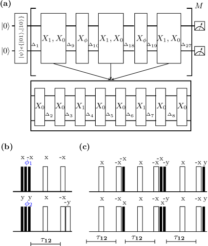
Figure 4.1: (a) Circuit diagram for the three-layer NUDD sequence. The innermost UDD layer consists of $X_{0}$ control pulses, the middle layer comprises $X_{1}$ control pulses and the outermost layer consists of $X_{\phi}$ pulses. The entire NUDD sequence is repeated $M$ times; $\Delta_{i}$ are time intervals. (b) NMR pulse sequence to implement the control pulses for $X_{0}$ and $X_{1}$ UDD sequences. The values of the rf pulse phases $\phi_{1}$ and $\phi_{2}$ are set to $x$ and $y$ for the $X_{0}$ and to $-x$ and $-y$ for the $X_{1}$ UDD sequence, respectively. (c) NMR pulse sequence to implement the control pulses for the $X_{\phi}$ UDD sequence. The filled rectangles denote $\pi/2$ pulses while the unfilled rectangles denote $\pi$ pulses, respectively. The time period $\tau_{12}$ is set to the value $(2J_{12})^{-1}$, where $J_{12}$ denotes the strength of the scalar coupling between the two qubits.

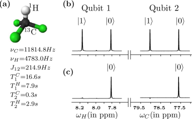
Figure 4.2: (a) Structure of isotopically enriched chloroform-¹³C molecule, with the ¹H spin labeling the first qubit and the ¹³C spin labeling the second qubit. The system parameters are tabulated alongside with chemical shifts $\nu_{i}$ and scalar coupling $J_{12}$ (in Hz) and NMR spin-lattice and spin-spin relaxation times $T_{1}$ and $T_{2}$ (in seconds). (b) NMR spectrum obtained after a $\pi/2$ readout pulse on the thermal equilibrium state and (c) NMR spectrum of the pseudopure $|00\rangle$ state. The resonance lines of each qubit in the spectra are labeled by the corresponding logical states of the other qubit.

4.3 Experimental protection of two qubits using NUDD

4.3.1 Experimental implementation of the NUDD scheme

We now turn to the NUDD implementation for $N=2$ on a two-qubit NMR system. The entire NUDD sequence can be written in terms of UDD control operators $X_{0},X_{1},X_{\phi}$ (defined in the previous section) and time evolution $U(\delta_{i}t)$ under the general Hamiltonian for time interval fractions $\delta_{i}$:

$$X_{c}(t) = U(\delta_{1}t)X_{0}U(\delta_{2}t)X_{0}U(\delta_{3}t)X_{1}U(\delta_{4}t)X_{0}U(\delta_{5}t)X_{0}$$ (4.24)

$$U(\delta_{6}t)X_{1}U(\delta_{7}t)X_{0}U(\delta_{8}t)X_{0}U(\delta_{9}t)X_{\phi}U(\delta_{10}t)X_{0}$$

$$U(\delta_{11}t)X_{0}U(\delta_{12}t)X_{1}U(\delta_{13}t)X_{0}U(\delta_{14}t)X_{0}U(\delta_{15}t)$$

$$X_{1}U(\delta_{16}t)X_{0}U(\delta_{17}t)X_{0}U(\delta_{18}t)X_{\phi}U(\delta_{19}t)$$

$$X_{0}U(\delta_{20}t)X_{0}U(\delta_{21}t)X_{1}U(\delta_{22}t)X_{0}U(\delta_{23}t)$$

$$X_{0}U(\delta_{24}t)X_{1}U(\delta_{25}t)X_{0}U(\delta_{26}t)X_{0}U(\delta_{27}t)$$

In our implementation, the number of $X_{0},X_{1}$ and $X_{\phi}$ control pulses used in one run of the three-layer NUDD sequence are 18, 6 and 2, respectively.

Using the UDD timing intervals defined above and applying the condition $\sum\delta_{i}=1$, their values are computed to be

$$\{\delta_{i}\} = \{\beta,2\beta,\beta,2\beta,4\beta,2\beta,\beta,2\beta,\beta,2\beta,4\beta,2\beta,4\beta,8\beta,$$ (4.25)

$$4\beta,2\beta,4\beta,2\beta,\beta,2\beta,\beta,2\beta,4\beta,2\beta,\beta,2\beta,\beta\}$$

where the intervals between the $X_{0},X_{1}$ and $X_{\phi}$ control pulses turn out to be a multiple of $\beta=0.015625$ .

The NUDD scheme for state protection and the corresponding NMR pulse sequence is given in Fig. 4.1. The unitary gates $X_{0}$, $X_{1}$, and $X_{\phi}$ drawn in Fig. 4.1(a) correspond to the UDD control operators already defined in the previous section. The $\Delta_{i}$ time interval in the circuit given in Fig. 4.1(a) is defined by $\Delta_{i}=\delta_{i}t$, using the $\delta_{i}$ given in Eqn. (4.25). The pulses on the top line in Figs. 4.1(b) and (c) are applied on the first qubit (¹H spin in Fig. 4.2), while those at the bottom are applied on the second qubit (¹³C spin in Fig. 4.2), respectively. All the pulses are spin-selective pulses, with the $90^{\circ}$ pulse length being $7.6\mu$s and $15.6\mu$s for the proton and carbon rf channels, respectively. When applying pulses simultaneously on both the carbon and proton spins, care was taken to ensure that the pulses are centered properly and the delay between two pulses was measured from the center of the pulse duration time. We note here that the NUDD schemes are experimentally demanding to implement as they contain long repetitive cycles of rf pulses applied simultaneously on both qubits and the timings of the UDD control sequences were matched carefully with the duty cycle of the rf probe being used.

We chose the chloroform-¹³C molecule as the two-qubit system to implement the NUDD sequence (Fig. 4.2 for details of system parameters and average NMR relaxation times of both the qubits). The two-qubit system Hamiltonian in the rotating frame (which includes the Hamiltonians $H_{S}$ and $H_{12}$ of Eqn. 4.3) is given by

$$H_{\rm rot}=2\pi[(\nu_{H}-\nu^{rf}_{H})I_{z}^{H}+(\nu_{C}-\nu^{rf}_{C})I_{z}^{C}+J_{12}I_{z}^{H}I_{z}^{C}]$$ (4.26)

where $\nu_{H}$ ($\nu_{C}$ ) is the chemical shift of the ${}^{1}H(^{13}C)$ spin, $\nu^{rf}_{i}$ is the rotating frame frequency ($\nu^{rf}_{i}=\nu_{i}$ for on-resonance), $I_{z}^{H}(I_{z}^{C})$ is the $z$ component of the spin angular momentum operator for the ${}^{1}H(^{13}C)$ spin, and $J_{12}$ is the spin-spin coupling constant.

Figure 4.3: Plot of fidelity versus time for (a) the $|01\rangle$ state and (b) the $|10\rangle)$ state, without any protection and after applying NUDD protection. The fidelity of both the states remains close to 1 for upto long times, after NUDD protection.

The two qubits were initialized into the pseudopure state $|00\rangle$ using the spatial averaging technique [177], with the corresponding density operator given by

$$\rho_{00}=\frac{1-\epsilon}{4}I+\epsilon|00\rangle\langle 00|$$ (4.27)

with a thermal polarization $\epsilon\approx 10^{-5}$ and $I$ being a $4\times 4$ identity operator. All experimental density matrices were reconstructed using quantum state tomography via a maximum likelihood protocol (Chapter 2). The experimentally created pseudopure state $|00\rangle$ was tomographed with a fidelity of $0.99$. The fidelity of an experimental density matrix was computed using Eq. (2.32).

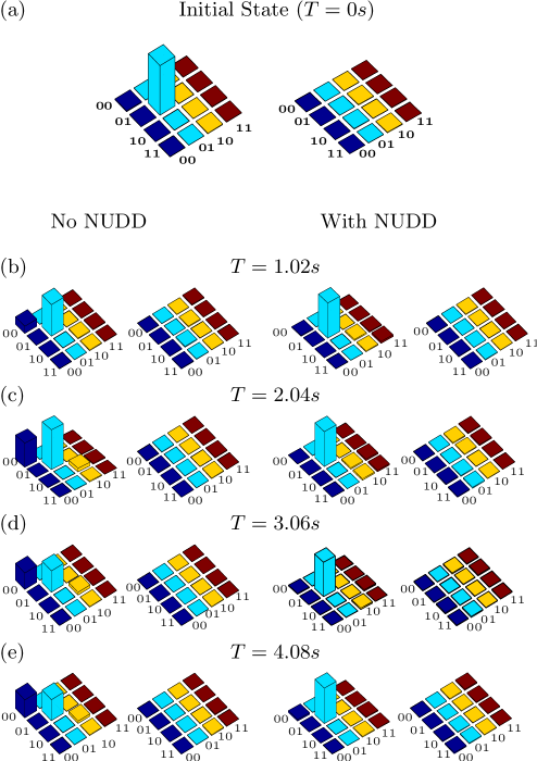
Figure 4.4: Real (left) and imaginary (right) parts of the experimental tomographs of the (a) $|01\rangle$ state, with a computed fidelity of 0.98. (b)-(e) depict the state at $T=1.02,2.04,3.06,4.08$ s, with the tomographs on the left and the right representing the state without any protection and after applying NUDD protection, respectively. The rows and columns are labeled in the computational basis ordered from $|00\rangle$ to $|11\rangle$.

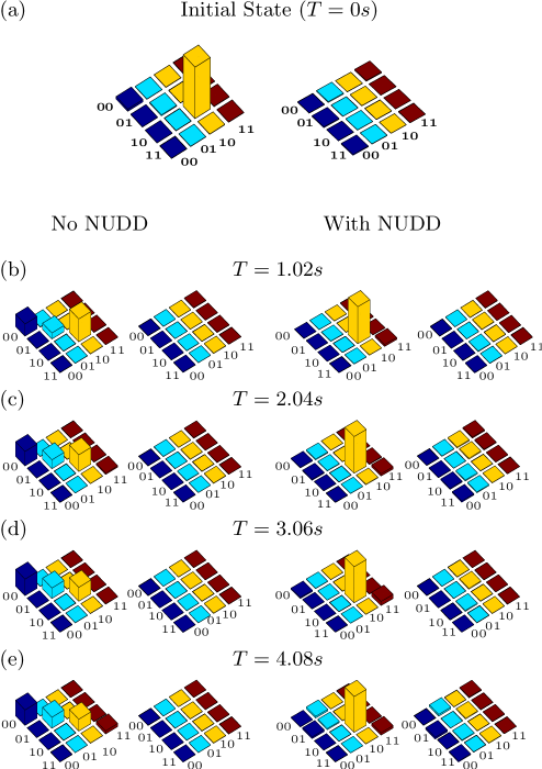
Figure 4.5: Real (left) and imaginary (right) parts of the experimental tomographs of the (a) $|10\rangle$ state, with a computed fidelity of 0.97. (b)-(e) depict the state at $T=1.02,2.04,3.06,4.08$ s, with the tomographs on the left and the right representing the state without any protection and after applying NUDD protection, respectively. The rows and columns are labeled in the computational basis ordered from $|00\rangle$ to $|11\rangle$.

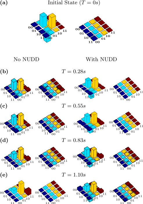
Figure 4.6: Real (left) and imaginary (right) parts of the experimental tomographs of the (a) $\frac{1}{\sqrt{2}}(|01\rangle-|10\rangle)$ state, with a computed fidelity of 0.99. (b)-(e) depict the state at $T=0.28,0.55,0.83,1.10$ s, with the tomographs on the left and the right representing the state without any protection and after applying NUDD protection, respectively. The rows and columns are labeled in the computational basis ordered from $|00\rangle$ to $|11\rangle$.

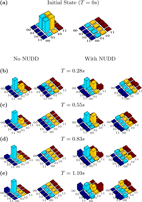
Figure 4.7: Real (left) and imaginary (right) parts of the experimental tomographs of the (a) $\frac{1}{\sqrt{2}}(|01\rangle+|10\rangle)$ state, with a computed fidelity of 0.99. (b)-(e) depict the state at $T=0.28,0.55,0.83,1.10$ s, with the tomographs on the left and the right representing the state without any protection and after applying NUDD protection, respectively. The rows and columns are labeled in the computational basis ordered from $|00\rangle$ to $|11\rangle$.

Figure 4.8: Plot of fidelity versus time for (a) the Bell singlet state and (b) the Bell triplet state, without any protection and after applying NUDD protection.

4.3.2 NUDD protection of known states in the subspace

We begin evaluating the efficiency of the NUDD scheme by first applying it to protect four known states in the two-dimensional subspace ${\cal P}$, namely two separable and two maximally entangled (Bell) states.

Protecting two-qubit separable states: We experimentally created the two-qubit separable states $|01\rangle$ and $|10\rangle$ from the initial state $|00\rangle$ by applying a $\pi_{x}$ on the second qubit and on the first qubit, respectively. The states were prepared with a fidelity of 0.98 and 0.97, respectively. One run of the NUDD sequence took 0.12756 s which included the time taken to implement the control operators, and $t=0.05$ s (as per Eqn. (4.24)). The entire NUDD sequence was applied 40 times. The state fidelity was computed at different time instants, without any protection and after applying NUDD protection. The state fidelity remains close to 0.9 for long times (upto 5 s) when NUDD is applied, whereas for no protection the $|01\rangle$ state loses its fidelity (fidelity approaches 0.5) after 3 s and the $|10\rangle$ state loses its fidelity after 2 s. A plot of state fidelities versus time is displayed in Fig. 4.3, demonstrating the remarkable efficacy of the NUDD sequence in protecting separable two-qubit states against decoherence. The signal attenuation has been ignored and the density matrix has been renormalized at every time point in Fig. 4.3, as described in Chap. 3,Sec. 3.3.2.3.

Figure 4.9: NMR pulse sequence for the preparation of arbitrary states. The sequence of pulses before the vertical dashed line achieve state initialization into the $|00\rangle$ state. The values of flip angles $\theta$ and $\phi$ of the rf pulses are the same as the $\theta$ and $\phi$ values describing a general state in the two-dimensional subspace ${\cal P}=\{|01\rangle,|10\rangle\}$. Filled and unfilled rectangles represent $\frac{\pi}{2}$ and $\pi$ pulses respectively, while all other rf pulses are labeled with their respective flip angles and phases; the interval $\tau_{12}$ is set to $(2J_{12})^{-1}$ where $J_{12}$ is the scalar coupling.

Protecting two-qubit Bell states: We next implemented NUDD protection on the maximally entangled singlet state $\frac{1}{\sqrt{2}}(|01\rangle-|10\rangle)$. We experimentally constructed the singlet state from the initial $|00\rangle$ state via the pulse sequence given in Fig. 4.9 with values of $\theta=-\frac{\pi}{2}$ and $\phi=0$. The fidelity of the experimentally constructed singlet state was computed to be 0.99.

One run of the NUDD sequence took 0.27756 s and $t$ was kept at $t=0.2$ s. The entire NUDD sequence was applied 4 times on the state. The singlet state fidelity at different time points was computed without any protection and after applying NUDD protection, and the state tomographs are displayed in Fig. 4.6. The signal attenuation has been ignored and the density matrix has been renormalized at every time point in Fig. 4.6. The fidelity of the singlet state remained close to 0.8 for 1 s when NUDD protection was applied, whereas when no protection is applied the state decoheres (fidelity approaches 0.5) after 0.55 s. We also implemented NUDD protection on the maximally entangled triplet state $\frac{1}{\sqrt{2}}(|01\rangle+|10\rangle)$. We experimentally constructed the triplet state from the initial $|00\rangle$ state via the pulse sequence given in Fig. 4.9 with values of $\theta=\frac{\pi}{2}$ and $\phi=0$. The fidelity of the experimentally constructed triplet state was computed to be 0.99. The total NUDD time was kept at $t=0.2$ s and one run of the NUDD sequence took 0.27756 s. The entire NUDD sequence was repeated 4 times on the state. The state fidelity at different time points was computed without any protection and after applying NUDD protection and the state tomographs are displayed in Fig. 4.7. The signal attenuation has been ignored and the density matrix has been renormalized at every time point in Fig. 4.7.

The fidelity of the triplet state remained close to 0.71 for 0.28 s when NUDD protection was applied, whereas when no protection is applied the state decoheres quite rapidly (fidelity approaches 0.5) after 0.28 s. A plot of state fidelities of both Bell states versus time is displayed in Fig. 4.8, In that the signal attenuation has been ignored and the density matrix has been renormalized at every time point. While the NUDD scheme was able to protect the singlet state quite well (the time for which the state remains protected is double as compared to its natural decay time), it is not able to extend the lifetime of the triplet state to any appreciable extent. What is worth noting here is the fact that the state fidelity remains considerably higher under NUDD protection compared to no protection, implying that there is a reduction in the “leakage” to other states.

4.3.3 NUDD protection of unknown states in the subspace

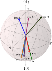
Figure 4.10: Geometrical representation of eight randomly generated states on a Bloch sphere belonging to the two-qubit subspace ${\cal P}=\{|01\rangle,|10\rangle\}$. Each vector makes angles $\theta,\phi$ with the $z$ and $x$ axes, respectively. The state labels RS-$i$ ($i=1..8$) are explained in the text.

We wanted to carry out an unbiased assessment of the efficacy of the NUDD scheme for state protection. To this end, we randomly generated several states in the two-dimensional subspace ${\cal P}$, and applied the NUDD sequence on each state.

Table 4.1: Results of applying NUDD protection on eight randomly generated states in the two-dimensional subspace. Each random state (RS) is tagged with a number for convenience, and its corresponding ($\theta$,$\phi$) angles are given in the column alongside. The fourth column displays the time at which the state fidelity approaches $\approx 0.8$ without NUDD protection and the last column displays the time for which state fidelity approaches $\approx 0.8$ after applying NUDD protection.

State	Label	$(\theta,\phi)$(deg)	Time (s)	Time (s)
			($F>0.8$)	($F>0.8$)
			Without NUDD	With NUDD
$0.29|01\rangle+(0.94+\iota 0.18)|10\rangle$	RS-1	(147,57)	0.1s	1.0s
$0.15|01\rangle-(0.76+\iota 0.63)|10\rangle$	RS-2	(163,349)	0.3s	1.1s
$0.98|01\rangle+(0.11-\iota 0.17)|10\rangle$	RS-3	(23,345)	0.1s	1.1s
$0.14|01\rangle+(0.36-\iota 0.92)|10\rangle$	RS-4	(164,175)	0.3s	1.1s
$0.99|01\rangle+(0.10+\iota 0.11)|10\rangle$	RS-5	(18,51)	0.3s	1.1s
$0.91|01\rangle+(0.22+\iota 0.36)|10\rangle$	RS-6	(50,152)	0.1s	0.9s
$0.07|01\rangle+(-0.77+\iota 0.64)|10\rangle$	RS-7	(172,285)	0.1s	1.1s
$0.06|01\rangle+(0.99-\iota 0.16)|10\rangle$	RS-8	(174,346)	0.3s	1.1s

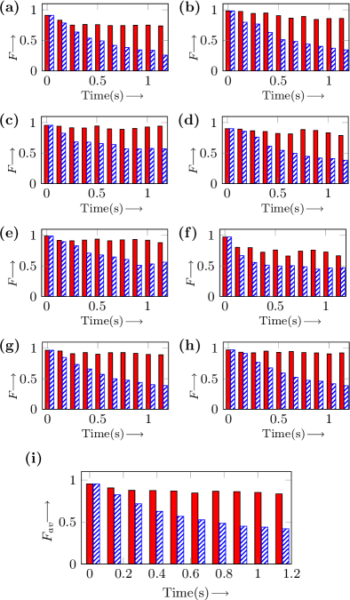
Figure 4.11: Bar plots of fidelity versus time of eight randomly generated states (labeled RS-$i$, $i=1..8$), without any protection (cross-hatched bars) and after applying NUDD protection (red solid bars): (a) RS-1, (b) RS-2, (c) RS-3, (d) RS-4, (e) RS-5, (f) RS-6, (g) RS-7 and (h) RS-8. (i) Bar plot showing average fidelity of all eight randomly generated states, at each time point.

A general state in the two-qubit subspace ${\cal P}=\{|01\rangle,|10\rangle\}$ can be written in the form

$$|\psi\rangle=\cos{\frac{\theta}{2}}|01\rangle+e^{-\iota\phi}\sin{\frac{\theta}{2}}|10\rangle\$$ (4.28)

These states were experimentally created by using the values of $\theta$ and $\phi$ (Eqn. (4.28)) as the flip angles of the rf pulses in the NMR pulse sequence (see Fig. 4.9 for visualization). The eight randomly generated representative two-qubit states are shown in Fig. 4.10. The entire three-layered NUDD sequence was applied 10 times on each of the eight random states. The time $t$ for the sequence was kept at $t=0.05$ s and one run of the NUDD sequence took $0.12756$ s. The plots of fidelity versus time are shown as bar graphs in Fig. 4.11, with the cross-hatched bars representing state fidelity without any protection and the solid bars representing state fidelity after NUDD protection. The signal attenuation has been ignored and the density matrix has been renormalized at every time point in Fig. 4.11. The final bar plot in Fig. 4.11(i) shows the average fidelity of all the randomly generated states at each time point. The results of protecting these random states via three-layered NUDD are tabulated in Table 4.1. Each state has been tagged by a label RS-$i$ (RS denoting “Random State” and $i=1,..8$), with its $\theta,\phi$ values displayed in the next column. The fourth column displays the values of the natural decoherence time (in seconds) of each state without NUDD protection, estimated by computing the time upto which state fidelity does not fall below 0.8. The last column in the table displays the time for which the state remains protected after applying NUDD, estimated by computing the time upto which state fidelity does not fall below 0.8. While the NUDD scheme is able to protect specific states in the subspace with varying degrees of success (as evidenced from the entries in the last column of in Table 4.1), on an average as seen from the bar plot of the average fidelity in Fig. 4.11(i), the scheme performs quite well.

4.4 Conclusions

In this chapter, a three-layer nested UDD sequence was experimentally implemented on an NMR quantum information processor and explored its efficiency in protecting arbitrary states in a two-dimensional subspace of two qubits. The nested UDD layers were applied in a particular sequence, and the full NUDD scheme was able to achieve second order decoupling of the system and bath. The scheme is sufficiently general as it does not assume prior information about the explicit form of the system-bath coupling. The experiments were highly demanding, with the control operations being complicated and involving manipulations of both qubits simultaneously. However, our results demonstrate that such systematic NUDD schemes can be experimentally implemented, and are able to protect multiqubit states in systems that are arbitrarily coupled to quantum baths.

In addition, to demonstrate that the NUDD scheme does not depend on the actual form of an initial superposition state. This scheme was applied to arbitrary states with randomly sampled coefficients and the experimental results shows that advantage of the NUDD schemes lies in the fact that one is sure that some amount of state protection will always be achieved. Furthermore, one need not know anything about the state to be protected or the nature of the quantum channel responsible for its decoherence. All one needs to know is the subspace to which the state belongs. In summary, if the QIP experimentalist has full knowledge of the state to be protected, it is better to use UDD schemes that are not nested. However, if there is only partial knowledge of the state, the QIP experimentalist would do better to use these “generic” NUDD schemes. If we do not know the subspace to which the state belongs, we need to consider the full space, which increases the number of nesting layers, and experimentally implementation becomes a difficult task. The study in this chapter points the way to the realistic protection of fragile quantum states up to high orders and against arbitrary noise.

Chapter 5 Experimentally preserving time-invariant discord using dynamical decoupling

5.1 Introduction

Interaction of quantum systems with their environment causes the destruction of intrinsic quantum properties such as quantum superposition, quantum entanglement and more general quantum correlations [178]. It has been observed that quantum entanglement may disappear completely but there still may exist quantum correlations in a quantum system. Quantum correlations are thus more fundamental than entanglement [179]. The quantification of quantum correlations, distinction from their classical counterparts, and their behavior under decoherence, is of paramount importance to quantum information processing [1]. Several measures of nonclassical correlations have been developed [179] and their signatures experimentally measured on an NMR setup [180, 181, 182]. Quantum discord is a measure of nonclassical correlations that are not accounted for by quantum entanglement [183]. While the intimate connection of quantum entanglement with quantum nonlocality is well understood and entanglement has long been considered a source of quantum computational speedup [184], the importance of quantum discord, its intrinsic quantumness and its potential use in quantum information processing protocols, is being explored in a number of contemporary studies [185].

A surprising recent finding suggests that for certain quantum states up to some time $\bar{t}$, quantum correlations are not destroyed by decoherence whereas classical correlations decay. After time $\bar{t}$ the situation is reversed and the quantum correlations begin to decay [186, 70]. This inherent immunity of such quantum correlations to environmental noise throws up new possibilities for the characterization of quantum behavior and its exploitation for quantum information processing. The peculiar “frozen” behavior of quantum discord in the presence of noise was experimentally investigated using photonic qubits [187] and NMR qubits [188, 189]. The class of initial quantum states that exhibit this sudden transition in their decay rates was theoretically studied under the action of standard noise channels, and it was inferred that the type of states that display such behavior depends on the nature of the decohering channel being considered [190]. Dynamical decoupling (DD) methods have been proposed to protect quantum discord from environment-induced errors [[191]] and a recent work showed that interestingly, DD schemes can also influence the timescale over which time-invariant quantum discord remains oblivious to decoherence [192].

In this chapter we demonstrate the remarkable preservation of time-invariant quantum discord upon applying time-symmetric DD schemes of the bang-bang variety, on a two-qubit NMR quantum information processor. We begin by looking at a measure for quantum and classical correlations for a special class of two-qubit quantum states, namely, Bell-diagonal (BD) states. Then the noise affecting a spin system is characterized by experimentally measuring the relaxation of the spins. Considering the spin system used which is a heteronuclear and the experimental results of the relaxation parameters, a model is proposed that the decoherence channel acting on the two qubits is mainly a phase damping channel acting independent on each qubit. According to this model zero quantum coherences and double quantum coherences decay with same rates which is equal to the sum of single quantum coherences decay rates. Experimental results validate this model. The BD state experimentally prepared, its decay is observed and found the quantum correlations freeze for a time interval. The results obtained from the experiments and theoretical noise model are compared. In the final section of this chapter, several robust DD sequences are applied to the system in the BD state, resulting in a significantly prolonged freezing time of quantum correlations.

5.2 Measure for correlations of two qubits

Consider a bipartite system made of an system A and B into a Hilbert space ${\cal H}_{A}\otimes{\cal H}_{B}$ with ${\cal H}_{A}$ and ${\cal H}_{B}$ is a Hilbert state of system A and B respectively. The total correlations of a state in a bipartite quantum system are measured by the quantum mutual information ${\cal I}(\rho_{AB})$ defined as

$${\cal I}(\rho_{AB})=S(\rho_{A})+S(\rho_{B})-S(\rho_{AB})$$ (5.1)

where $S(\rho)=-\mathrm{Tr}\{\ \rho\log_{2}\rho\ \}$ is the von Neumann entropy.

Then the quantum discord is defined as

$${\cal D}(\rho_{AB})={\cal I}(\rho_{AB})-{\cal C}(\rho_{AB})$$ (5.2)

where ${\cal C}(\rho_{AB})$ is a classical correlations of the state [70, 193]. Next we specify the quantity used for measuring the classical correlations. Such a quantity is based on the generalization of the concept of conditional entropy. We know that performing measurements on system B affects our knowledge of system A. How much system A is modified by a measurement of B depends on the type of measurement performed on B. Here the measurement is considered of von Neumann type. It is described by a complete set of orthonormal projectors $\{\Pi_{k}\}$ on subsystem B corresponding to the outcome k. The classical correlations ${\cal{C}}{(\rho_{AB})}$ are then defined as

$${\cal{C}}(\rho_{AB})=\max_{\{\varPi_{k}\}}[S(\rho_{A})-S(\rho_{\rho_{A}}|\{\varPi_{k}\})]$$ (5.3)

where the maximum is taken over the set of the projective measurements $\{\varPi_{k}\}$ and $S(\rho_{\rho_{A}}|\{\varPi_{k}\})=\sum_{k}p_{k}S(\rho_{k})$ is the conditional entropy of A, given the knowledge of the state of B, with $p_{k}=\mathrm{Tr}_{AB}(\rho_{AB}\varPi_{k})$ and $\rho_{k}=\mathrm{Tr}_{B}(\varPi_{k}\rho_{AB}\varPi_{k})/p_{k}$.

Consider a two-qubit quantum system with its state space spanned by the states $\{|00\rangle,|01\rangle,$ $|10\rangle,|11\rangle\}$ and the eigenstates of the Pauli operators $\sigma_{z}^{1}\otimes\sigma_{z}^{2}$. Any state for such a system is locally equivalent to

$$\rho=\frac{1}{4}\left(I+\vec{a}.\vec{\sigma}\otimes{I}+I\otimes\vec{b}.\vec{\sigma}+\sum^{3}_{j=1}c_{j}\sigma_{j}\otimes\sigma_{j}\right)$$ (5.4)

where ${I}$ is the identity operator, $\vec{\sigma}=(\sigma_{x},\sigma_{y},\sigma_{z})$ with Pauli spin observables in the $x$,$y$,$z$ direction, $\vec{u}=(u_{x},u_{y},u_{z})$ $\in$ $R^{3}$, $\vec{u}\vec{\sigma}=u_{x}\sigma_{x}+u_{y}\sigma_{y}+u_{z}\sigma_{z}$ ($u=a,b,c$) . Here we are only interested in the family of BD states which is described by a density matrix

$$\rho_{AB}=\frac{1}{4}\left({I}+\sum_{j=1}^{3}c_{j}\sigma_{j}\otimes\sigma_{j}\right)$$ (5.5)

where $c_{j}$ are real constants such that $\rho_{AB}$ is a valid density operator. The eigenvalues of the density matrix $\rho_{AB}$ are given by

$$\lambda_{0} = \frac{1}{4}(1-c_{1}-c_{2}-c_{3}),$$

$$\lambda_{1} = \frac{1}{4}(1-c_{1}+c_{2}+c_{3}),$$

$$\lambda_{2} = \frac{1}{4}(1+c_{1}-c_{2}+c_{3}),$$

$$\lambda_{3} = \frac{1}{4}(1+c_{1}+c_{2}-c_{3}).$$

The reduced density matrices of $\rho_{AB}$ as given in Eq. 5.5 are $\rho_{A}=\frac{{I}}{2}$ and $\rho_{B}=\frac{{I}}{2}$. The total correlations $\cal{I}(\rho)$ are given by:

$${\cal{I}(\rho)}=2+\sum_{l=0}^{3}\lambda_{l}\log_{2}\lambda_{l}$$ (5.7)

The classical correlations for the BD states given as

$${\cal C}[\rho_{AB}]=\sum_{j=1}^{2}\frac{1+(-1)^{j}\chi}{2}\log_{2}[1+(-1)^{j}\chi],$$ (5.8)

where $\chi=\max\{|c_{1}|,|c_{2}|,|c_{3}|\}$. The maximization procedure with respect to the projective measurements, present in the definition of the classical correlations of Eq.(5.3), can be performed explicitly for the system here considered noticing that the complete set of the orthogonal projectors is given by $\varPi_{j}=|\theta_{j}\rangle\langle\theta_{j}|$, with j=1,2, $|\theta_{1}\rangle={\rm cos}\theta|0\rangle+e^{-i\phi}{\rm sin}\theta|1\rangle$, $|\theta_{2}\rangle={\rm sin}\theta|0\rangle+e^{-i\phi}{\rm cos}\theta|1\rangle$, and the state of the system always remains of the form given by Eq.(5.5) during time evolution [70].

5.3 Characterization of noise channels

In high field NMR, the Zeeman interaction causes a splitting of the energy levels according to the field direction and the difference between magnetic quantum numbers

$$\Delta m_{rs}=m_{r}-m_{s}$$ (5.9)

defines the order of the coherence. If $\Delta m_{rs}=0$ the coherence is a zero quantum (ZQ) coherence, if $\Delta m_{rs}=\pm 1$ the coherence is a single quantum (SQ) coherence, and if $\Delta m_{rs}=\pm 2$ the coherence is a double quantum (DQ) coherence. In general, a density matrix element $\rho_{rs}$ represents $p$-quantum coherence $(p=m_{r}-m_{s})$ [23, 97]. For our two-qubit system we use for the experiments, the experimentally measured longitudinal NMR spin relaxation times are ${T}_{1}^{\rm H}\approx 7.9$ s and ${T}_{1}^{\rm C}\approx$ 16.6 s, which are much longer than the measured effective NMR transverse spin relaxation rates ${T}_{2}^{\rm H}$ = $0.513\pm 0.01$ s and ${T}_{2}^{\rm C}=0.193\pm 0.005$ s. Since we study the decoherence of the state for an evolution time of approximately 0.5 s, we neglect the effects of the amplitude-damping channel whose effects are associated with ${T}_{1}$ and assume that the main noise channel for our system is the phase-damping channel. The effective transverse spin relaxation rates were measured by applying a $90^{\circ}$ excitation pulse followed by a decay interval (with no refocusing pulse) and by fitting the resulting decay of the magnetization. The decay rate of SQ coherence of spin(i) is given by $1/T_{2}^{i}$. Our experimental system is heteronuclear, with two different nuclear species (proton and carbon), having very different Larmor resonance frequencies and hence large chemical shift differences. We hence hypothesize that each spin decoheres in an independent phase damping channel which is not correlated with that of the other spin. Therefore, we model the phase damping channel for this system as a homogeneous dephasing channel acting independently on each qubit [194]. We use the operator-sum representation formalism and the associated phase-damping Kraus operators [1].The Kraus operators for a two-qubit system under phase damping channel are:

$$E_{1}(t) = \frac{1}{2}(1+e^{-\gamma_{1}t})^{\frac{1}{2}}(1+e^{-\gamma_{2}t})^{\frac{1}{2}}I\otimes I,$$

$$E_{2}(t) = \frac{1}{2}(1+e^{-\gamma_{1}t})^{\frac{1}{2}}(1-e^{-\gamma_{2}t})^{\frac{1}{2}}I\otimes\sigma_{z},$$

$$E_{3}(t) = \frac{1}{2}(1-e^{-\gamma_{1}t})^{\frac{1}{2}}(1+e^{-\gamma_{2}t})^{\frac{1}{2}}\sigma_{z}\otimes I,$$

$$E_{4}(t) = \frac{1}{2}(1-e^{-\gamma_{1}t})^{\frac{1}{2}}(1-e^{-\gamma_{2}t})^{\frac{1}{2}}\sigma_{z}\otimes\sigma_{z},$$ (5.10)

where $\gamma_{1}=1/T^{i}_{2}$ is the decay constant of the $i^{th}$ spin, $I$ is the identity matrix and $\sigma_{z}$ is a Pauli matrix.

$${\sum_{j}E_{j}(t)E_{j}(t)^{\dagger}}=1,$$ (5.11)

$$\rho_{BD}(t)=\sum_{j}E_{j}(t)\rho_{AB}(0)E_{j}(t)^{\dagger}.$$ (5.12)

Once we fix the model, we can apply it to any state. One of the qualitative predictions of the model is that the DQ and ZQ decay rates are equal. We measured these rates in two independent experiments and compared them with those predicted by the above model (whose parameters are completely fixed). The experimentally measured DQ and ZQ decay rates were $\gamma_{DQ}=6.395\pm 0.23$ s^-1 and $\gamma_{ZQ}=6.138\pm 0.275$ s^-1 respectively, and the theoretically predicted common decay was $\gamma_{1}+\gamma_{2}=\frac{1}{T^{H}_{2}}+\frac{1}{T^{C}_{2}}=7.21\pm 0.173$ s^-1, showing the model works.

5.3.1 Bell-diagonal states under a dephasing channel

For a two-qubit system where each qubit is affected by an independent local dephasing channel, to see the evolution under the phase-damping channel acting independently on each qubit, we use the operator-sum representation formalism and the associated phase-damping Kraus operators [1]. The evolution in a noisy environment is governed by the phase-damping channel in Eq. (5.3), and it turns out for Bell-diagonal states $\rho_{AB}$

$$c_{1}(t) = c_{1}(0)exp[-(\gamma_{1}+\gamma_{2})t],$$

$$c_{2}(t) = c_{2}(0)exp[-(\gamma_{1}+\gamma_{2})t],$$

$$c_{3}(t) = c_{3}(0).$$ (5.13)

5.4 Time invariant quantum correlations

We now consider a system in the special class of Bell-diagonal states for which $c_{1}(0)=\pm 1$ and $c_{2}(0)=\mp c_{3}(0)$, with $|c_{3}|<1$ under the dephasing channel as define above in Eq.  (5.3). At time $t$ the total correlations are given by

$${{\cal I}[\rho_{AB}(t)]} = \sum_{j=1}^{2}\frac{1+(-1)^{j}c_{3}(t)}{2}\log_{2}[1+(-1)^{j}c_{3}(t)]+$$ (5.14)

$$\sum_{j=1}^{2}\frac{1+(-1)^{j}c_{1}(t)}{2}\log_{2}[1+(-1)^{j}c_{1}(t)],$$

the classical correlations are given by

$${{\cal C}[\rho_{AB}(t)]}=\sum_{j=1}^{2}\frac{1+(-1)^{j}\chi(t)}{2}\log_{2}[1+(-1)^{j}\chi(t)],$$ (5.15)

where $\chi(t)=\max\{|c_{1}(t)|,|c_{2}(t)|,|c_{3}(t)|\}$, and the quantum correlations are given by

$${\cal D}[\rho_{AB}(t)]={\cal I}[\rho_{AB}(t)]-{\cal C}[\rho_{AB}(t)].$$ (5.16)

We can see that since our system is mainly affected by the phase damping channel, for

$$t<\bar{t}=-\frac{ln(|c_{3}|)}{2\gamma}$$ (5.17)

quantum correlations remain constant

$${{\cal D}[\rho_{AB}(t<\bar{t})]}=\sum_{j=1}^{2}\frac{1+(-1)^{j}c_{3}(0)}{2}\log_{2}[1+(-1)^{j}c_{3}(0)],$$ (5.18)

and after $t>\bar{t}$ the quantum correlations start decreasing towards zero and the classical correlations of system remain constant which is given by:

$${{\cal C}[\rho_{AB}(t>\bar{t})]}=\sum_{j=1}^{2}\frac{1+(-1)^{j}c_{3}(0)}{2}\log_{2}[1+(-1)^{j}c_{3}(0)].$$ (5.19)

5.5 Experimental realization of time-invariant discord

5.5.1 NMR System

We create and preserve time-invariant discord in a two-qubit NMR system of chloroform-¹³C, with the ¹H and ¹³C nuclear spins encoding the two qubits (Fig. 4.2). The ensemble of nuclear spins is placed in a longitudinal strong static magnetic field ($B_{0}\approx 14.1$T) oriented along the $z$ direction. The ¹H and ¹³C nuclear spins precess around $B_{0}$ at Larmor frequencies of $\approx 600$ MHz and $\approx 150$ MHz, respectively. The evolution of spin magnetization is controlled by applying rf-field pulses in the $x$ and $y$ directions. The internal Hamiltonian of the system in the rotating frame is given by Eq.(4.26)

The two-qubit system was initialized into the pseudopure state $|00\rangle$ by the spatial averaging technique [24]. Density matrices were reconstructed from experimental data by using a reduced set of quantum state tomography (QST) operations combined with the maximum likelihood method [59] as described in Chapter 2 to avoid any negative eigen values. The fidelity $F$ of all the experimental density matrices reconstructed in this work was computed using the Eq.(2.32). The experimentally created pseudopure state $|00\rangle$ was tomographed with a fidelity of $0.99$, and the NMR signal of this state was used as a reference for computation of state fidelity in all subsequent time-invariant discord experiments.

5.5.2 Observing time-invariant discord

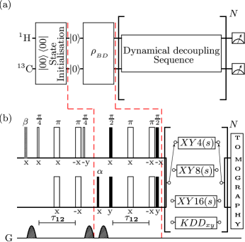
Figure 5.1: (a) Quantum circuit for the initial pseudopure state preparation, followed by the block for BD state preparation. The next block depicts the DD scheme used to preserve quantum discord. The entire DD sequence is repeated $N$ times before measurement. (b) NMR pulse sequence corresponding to the quantum circuit. The rf pulse flip angles are set to $\alpha=46^{\circ}$ and $\beta=59.81^{\circ}$, while all other pulses are labeled with their respective angles and phases.

A class of Bell-diagonal (BD) states with maximally mixed marginals defined in terms of Pauli operators $\sigma_{i}$ are

$$\rho_{\rm BD}=\frac{1}{4}\left(\,{I}\right.+{\sum_{i=1}^{3}}\left.c_{i}\ \sigma_{i}\otimes\sigma_{i}\right)$$ (5.20)

where the coefficients $c_{i}$ with $0\leq|c_{i}|\leq 1$ determine the state completely and can be computed as $c_{i}=\langle\sigma_{i}\otimes\sigma_{i}\rangle$.

We aim to prepare an initial BD state with the parameters $c_{1}(0)=1$, $c_{2}(0)=0.7$, $c_{3}(0)=-0.7$. The NMR pulse sequence for the preparation of this state from the $|00\rangle$ pseudopure state is given in Fig. 5.1(b). Preparing the BD state involves manipulation of NMR multiple-quantum coherences by applying rotations in the zero-quantum and double-quantum spin magnetization subspaces. Since the molecule is a heteronuclear spin system, high-power, short-duration rf pulses were used for gate implementation (with rf pulses of flip angles $\alpha=45.57^{\circ}$ and $\beta=59.81^{\circ}$ in Fig. 5.1 having pulse lengths of $6.85\mu$s and $5.02\mu$s, respectively). The experimentally achieved $\rho^{\rm E}_{\rm BD}$ (reconstructed using the maximum likelihood method [59] had parameters $c_{1}(0)=1.0$, $c_{2}(0)=0.680$ and $c_{3}(0)=-0.680$ and a computed fidelity of $0.99$. The experimentally reconstructed density matrix (using quantum state tomography and maximum likelihood) was found to be:

$\mathbf{\rho^{\rm E}_{\rm BD}}==\left(\begin{array}[]{cccc}0.080&0.003+0.000i&0.003+0.000i&0.080+0.000i\\ 0.003-0.000i&0.420&0.420+0.001i&0.003+0.000i\\ 0.003-0.000i&0.420-0.001i&0.420&0.003+0.000i\\ 0.080-0.000i&0.003-0.000i&0.003-0.000i&0.080\\ \end{array}\right)$

Correlation functions for the BD states can be computed readily to give the classical correlations (${\cal C}[\rho(t)]$), the quantum discord (${\cal D}[\rho(t)]$), and total correlations (${\cal I}[\rho(t)]$ [70]:

$${\cal C}[\rho(t)] = \sum_{j=1}^{2}\frac{1+(-1)^{j}\chi(t)}{2}\log_{2}[1+(-1)^{j}\chi(t)]$$

$${\cal I}[\rho(t)] = \sum_{j=1}^{2}\frac{1+(-1)^{j}c_{1}(t)}{2}\log_{2}[1+(-1)^{j}c_{1}(t)]$$

$$+\sum_{j=1}^{2}\frac{1+(-1)^{j}c_{3}}{2}\log_{2}[1+(-1)^{j}c_{3}]$$

$${\cal D}(\rho) \equiv {\cal I}(\rho)-{\cal C}(\rho)$$ (5.21)

where $\chi(t)=\max\{|c_{1}(t)|,|c_{2}(t)|,|c_{3}(t)|\}$.

For the class of BD states with coefficients $c_{1}=\pm 1,c_{2}=\mp c_{3},|c_{3}|<1$, the evolution under a noisy environment is governed by the noise operators given in Eq.5.3, and it turns out that $c_{1}(t)=c_{1}(0)exp{[-(\gamma_{1}+\gamma_{2})t]},c_{2}(t)=c_{2}(0)exp{[-(\gamma_{1}+\gamma_{2})t]}$, $c_{3}(0)\equiv c_{3}$, and the quantum discord does not decay up to some finite time $\bar{t}$ [70]. Initially ($t=0$), the computed correlations in the $\rho^{\rm E}_{\rm BD}$ state (taken as an average of five density matrices initially prepared in the same state) turned out to be ${\cal C}[\rho(0)]=0.999\pm 0.169$, ${\cal D}[\rho(0)]=0.366\pm 0.024$ and ${\cal I}[\rho(0)]=1.366\pm 0.017$. The simulated and experimental plots of the dynamics of the quantum discord, classical correlations and total correlations are shown in Fig.5.2 (a) and (b) respectively, and shows a distinct transition from the classical to the quantum decoherence regimes at $t=\bar{t}$. The transition time up to which quantum discord remains constant is $\bar{t}=\frac{1}{2\gamma}\ln\left|\frac{c_{1}(0)}{c_{3}(0)}\right|$.

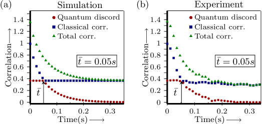
Figure 5.2: Time evolution of total correlations (triangles), classical correlations (squares) and quantum discord (circles) of the BD state: (a) Simulation, (b) Experimental plot without applying any preservation.

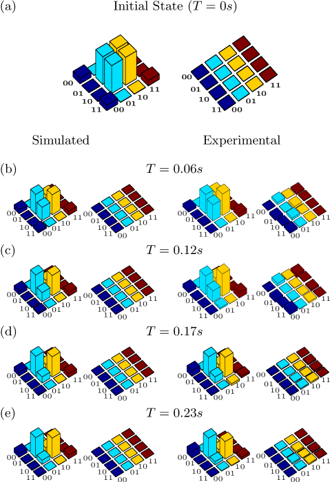
Figure 5.3: Real (left) and imaginary (right) parts of the experimental tomographs of the (a) Bell Diagonal (BD) state, with a computed fidelity of 0.99. (b)-(e) depict the state at $T=0.06,0.12,0.17,0.23$s, with the tomographs on the left and the right representing the simulated and experimental state, respectively. The rows and columns are labeled in the computational basis ordered from $|00\rangle$ to $|11\rangle$.

We allowed the experimentally prepared state $\rho^{\rm E}_{\rm BD}$, to evolve freely in time and determined the parameters $c_{i}$ at each time point. We used these experimentally determined coefficients to compute the classical correlations (${\cal C}[\rho(t)]$), the quantum discord (${\cal D}[\rho(t)]$), and total correlations (${\cal I}[\rho(t)]$) at each time point. The transition time up to which quantum discord remains constant was experimentally determined to be $\bar{t}=0.052$s. The experimental results correlate well with the theoretical noise model which allows to calculate $\bar{t}$ and the value comes out to be 0.054 s. The tomographed density matrix, reconstructed at different time points, shows that state evolution remains confined to the subspace of BD states, as is evident from the experimentally reconstructed density matrices of the state at different time points displayed in Fig.5.3.

5.6 Protection of time-invariant discord using dynamical decoupling schemes

DD schemes, consisting of repeated sets of $\pi$ pulses with tailored inter-pulse delays and phases, have played an important role in dealing with the debilitating effects of decoherence [166]. Several NMR QIP experiments have successfully used DD-type schemes to preserve quantum states [195, 63]. These schemes are expected to provide an advantage over traditional Carr-Purcell-Meiboom-Gill (CPMG) refocusing schemes and here we compared the two experimentally.

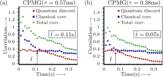
Figure 5.4: Time evolution of total correlations (triangles), classical correlations (squares) and quantum discord (circles) of the BD state: Experimental plots using CPMG preserving sequences (a) CPMG with $\tau=0.57$ ms and (b) CPMG with $\tau=0.38$ ms.

We first protect these states and their related quantum correlations using standard CPMG schemes of the type ($\tau-\pi-\tau-\pi$). The results are shown in Fig.5.4(a) and (b) for two different values of $\tau$ (the time interval between two consecutive $\pi$ pulses). It turns out that the CPMG schemes which are based on the traditional Hahn spin echo are able to provide protection to some extent and the life time of the time invariant quantum discord grows from 0.05 s to 0.11 s as we increase the number of $\pi$ pulses. However, as we try to increase the number of $\pi$ pulses further the results are counter-productive as shown in Fig.5.4(b). Therefore, beyond a point we have to give up the standard Hahn spin echo strategy.

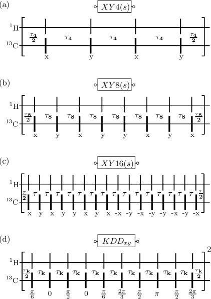
Figure 5.5: NMR pulse sequence corresponding to DD schemes (a) XY4(s), (b) XY8(s), (c) XY16(s), and (d) KDD_xy , with time delays between pulses denoted by $\tau_{4}$ , $\tau_{8}$, $\tau$, $\tau_{k}$ , respectively. All the pulses are of flip angle $\pi$ and are labeled with their respective phases. The pulses are applied simultaneously on both qubits. The superscript ‘2’ in the KDD xy sequence denotes that one unit cycle of this sequence contains two blocks of the ten-pulse block represented schematically, i.e., a total of twenty pulses. The shorter duration proton pulses and the longer duration carbon pulses are centered on each other and the various time delays ($\tau_{4}$, $\tau_{8}$ , $\tau$, $\tau_{k}$) in all the DD schemes are tailored to the gap between two consecutive carbon pulses.

Next we implemented more sophisticated DD sequences to explore if we can further protect the BD state, and hence the related quantum correlations typified via the survival time of the quantum discord $\bar{t}$. If the $\pi$ pulses in a DD sequence are non-ideal (either due to finite pulse lengths or flip angle and off-resonant driving errors), it leads to imperfect system-bath decoupling. Several schemes have been designed to make DD sequences robust against pulse imperfections by achieving ideal pulse rotations. Standard CPMG-based DD sequences used $\pi$ pulses applied along the same rotation axis, which then preserve coherence along only one spin component. The XY family of DD sequences applies pulses along two orthogonal ($x$, $y$) axes, which preserves coherences about both spin rotation axes. The basic XY4(s) DD sequence is a four-pulse sequence with phases $x-y-x-y$, with pulses applied at the center of each time period such that the whole sequence is time-symmetric with respect to its center [68]. The XY8(s) DD sequence uses the XY4(s) sequence as a building block, by combining the XY4(s) sequence with its time-reversed version, so that the whole eight-pulse sequence is explicitly time-symmetric. Each cycle of the symmetrized DD sequences is applied several times to achieve higher-order decoupling [172]. The Knill dynamical decoupling (KDD) sequence combines the rotation pattern of the XY4(s) sequence with composite pulses, replacing each $\pi$ pulse in the DD sequence with a composite sequence of five pulses with different phases [[172]]:

$${\rm KDD}_{\phi}=(\pi)_{\pi/6+\phi}-(\pi)_{\phi}-(\pi)_{\pi/2+\phi}-(\pi)_{\phi}-(\pi)_{\pi/6+\phi}.$$ (5.22)

The additional phases in the KDD_xy ($xy$ in the subscript denoting pulses applied along both axes) lead to better compensation for pulse errors, combining two of the basic five-pulse blocks given in Eq.(5.22) that are shifted in phase by $\frac{\pi}{2}$ i.e [KDD₀-KDD${}_{\frac{\pi}{2}}$]. The four symmetrized DD schemes used in our experiments to preserve time- invariant discord, namely XY4(s), XY8(s), XY16(s) and KDD_xy , are schematically represented in Fig.5.5. The ‘2’ in the superscript of the KDD_xy scheme denotes that one unit cycle of this scheme contains two of ten-pulse blocks, for a total of twenty pulses. We applied $\pi$ pulses simultaneously on both spins, with pulse lengths of $15.1$ $\mu$s and $26.8$ $\mu$s for the proton and carbon spins, respectively. The proton and carbon pulses are centered on each other and the time delay between pulses was set at the gap between two consecutive carbon pulses. Each DD sequence was applied a repeated number of times (N being as large as experimentally possible), for good coherence preservation.

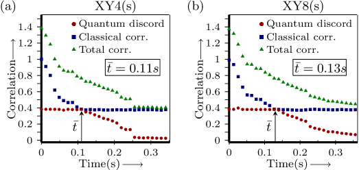
Figure 5.6: Time evolution of total correlations (triangles), classical correlations (squares) and quantum discord (circles) of the BD state: Experimental plots using (a) XY4(s) with $\tau_{4}=0.58$ ms and (b) XY8(s) with $\tau_{8}=0.29$ ms.

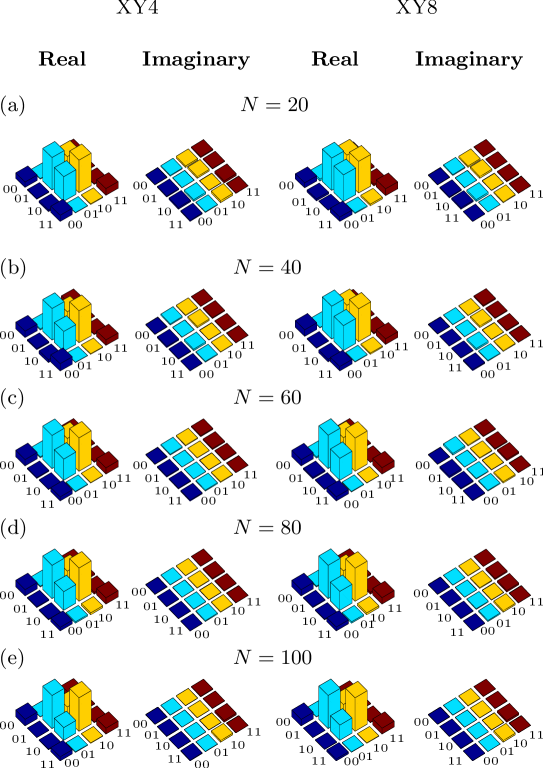
Figure 5.7: Real (left) and imaginary (right) parts of the experimental tomographs of the (a)-(e) depict the BD state at $N=20,40,60,80,100$, with the tomographs on the left and the right representing the BD state after applying the XY4 and XY8 scheme, respectively. The rows and columns are labeled in the computational basis ordered from $|00\rangle$ to $|11\rangle$.

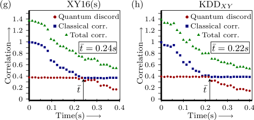
Figure 5.8: Time evolution of total correlations (triangles), classical correlations (squares) and quantum discord (circles) of the BD state: Experimental plots using (a) XY16(s) with $\tau=0.145$ ms and (b) KDD_xy with $\tau_{k}=0.116$ ms.

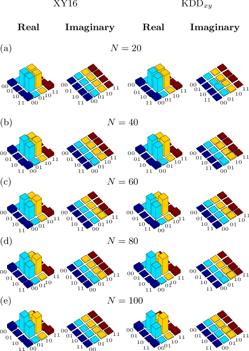
Figure 5.9: Real (left) and imaginary (right) parts of the experimental tomographs in (a)-(e) depict the Bell Diagonal (BD) state at $N=20,40,60,80,100$, with the tomographs on the left and the right representing the BD state after applying the XY16 and KDD_xy preserving DD schemes, respectively. The rows and columns are labeled in the computational basis ordered from $|00\rangle$ to $|11\rangle$.

We implemented the symmetrized XY4(s) DD scheme for $\tau_{4}=0.58$ ms and an experimental time for one run of $2.43$ ms. The time for which quantum discord persists using the XY4(s) scheme is $\bar{t}=0.11$ s, which is double the time as compared to ‘no-preservation’ (Fig. 5.6(a)). We implemented the XY8(s) DD scheme for $\tau_{8}=0.29$ ms and an experimental time for one run of 2.52 ms. The time for which quantum discord persists using the XY8(s) scheme is $\bar{t}=0.13s$, nearly the same as the XY4(s) scheme (Fig. 5.6(b)). The XY16(s) DD scheme provides even better compensation than the XY8(s) sequence. We implemented the XY16(s) scheme for $\tau=0.145$ ms and an experimental time for one run of $2.75$ ms. The time for which quantum discord persists for the XY16(s) scheme is $\bar{t}=0.24$ s, which is four times the persistence time of the discord when no preservation is applied (Fig.5.8(a)). We implemented the KDD$xy$ sequence with $\tau=0.116$ ms and an experimental time for one run of 2.86 ms. In this case too, the time for which quantum discord persists $\bar{t}=0.22$ s is quadrupled, as compared to no-preservation (Fig.5.8(b)). The $\tau$ delays are chosen in such a way that for a given sequence the protection is maximum. If we decrease $\tau$ delay intervals further, errors due to $\pi$ pulses dominates. The DD sequence was looped for five times between each time point in Figs.5.4, 5.6 and 5.8, which typically means repeating a DD sequence 175-200 times during an experiment covering all time points. The experimental tomographs of the BD state at different instances of time after using XY4(s), XY8(s), XY16(s) and KDD_xy DD preservation schemes to protect time-invariant discord are given in  Fig.5.7 and  Fig.5.9. All the experimental tomographs display excellent preservation of the state, with very little leakage.

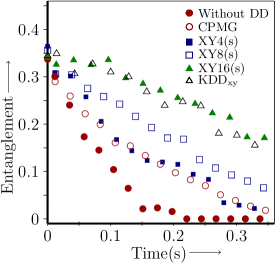
Figure 5.10: Plot of time evolution of entanglement without applying any preservation (filled circle), CPMG with $\tau=0.57$ ms (empty circle), XY4(s) (filled rectangle), XY8(s) (empty rectangle), XY16(s) (filled triangle) and KDD_xy (empty triangle),respectively.

In  Fig.5.10, we plotted the protection of quantum entanglement in the two-qubit BD state via CPMG and DD schemes, using negativity as an entanglement measure. It turns out that the results of entanglement protection are similar to that of discord protection namely, that CPMG and XY4(s) schemes protect entanglement to some extent while the more involved DD schemes are able to protect entanglement for relatively long times up to 0.3 s (as compared to its natural decay time of 0.12 s without any DD protection). However, the phenomenon of freezing of entanglement is not observed, unlike the case for quantum discord.

5.6.1 Conclusions

The two-qubit system we used in our experiments is mainly affected by an independent phase damping channel on each qubit for the experimental time regime under consideration. One of the main sources of relaxation in NMR is dipolar relaxation. Such noise can be ideally suppressed by the CPMG sequence. The suppression of noise is expected to increase by reducing the delay between the $\pi$ pulses, but due to imperfect $\pi$ pulses after a certain time point instead of suppressing noise, starts contributing to the noise. Also, the CPMG sequence is designed to protect magnetization along one particular axis, not for a general axis. To mitigate all these problems we used XY4(s), XY8(s), XY16(s) and KDD_xy DD sequences, which are robust against these imperfections and protect magnetization along the general axis. Our results show that time-invariant quantum discord, which remains unaffected under certain decoherence regimes, can be preserved for very long times using DD schemes. Our experiments have important implications in situations where persistent quantum correlations have to be maintained to carry out quantum information processing tasks.

Chapter 6 Dynamics of tripartite entanglement under decoherence and protection using dynamical decoupling

6.1 Introduction

In Chapter 5, we considered the situation where we have knowledge of the state of the system as well as its interaction with the environment. In such situations, since the noise model is known, decoupling strategies can be designed to cancel this noise. Using these decoupling strategies, we experimentally extended the lifetime of time invariant discord of two-qubit Bell-diagonal states. In this chapter we extend the same idea for experimental preservation of three-qubit entangled states. Quantum entanglement is considered to lie at the crux of QIP [1] and while two-qubit entanglement can be completely characterized, multipartite entanglement is more difficult to quantify and is the subject of much recent research [184]. Entanglement can be rather fragile under decoherence and various multiparty entangled states behave very differently under the same decohering channel [196]. It is hence of paramount importance to understand and control the dynamics of multipartite entangled states in multivarious noisy environments [197, 198, 199]. A three-qubit system is a good model system to study the diverse response of multipartite entangled states to decoherence and the entanglement dynamics of three-qubit GHZ and W states have been theoretically well studied [200, 201]. Under an arbitrary (Markovian) decohering environment, it was shown that W states are more robust than GHZ states for certain kinds of channels while the reverse is true for other kinds of channels [202, 203, 204, 205].

On the experimental front, tripartite entanglement was generated using photonic qubits and the robustness of W state entanglement was studied in optical systems [206, 207, 208, 209]. The dynamics of multi-qubit entanglement under the influence of decoherence was experimentally characterized using a string of trapped ions [210] and in superconducting qubits [211]. In the context of NMR quantum information processing, three-qubit entangled states were experimentally prepared [212, 138, 28, 213], and their decay rates compared with bipartite entangled states [43].

With a view to protecting entanglement, dynamical decoupling (DD) schemes have been successfully applied to decouple a multiqubit system from both transverse dephasing and longitudinal relaxation baths [105, 152, 173, 65]. UDD schemes have been used in the context of entanglement preservation [214, 215], and it was shown theoretically that Uhrig DD schemes are able to preserve the entanglement of two-qubit Bell states and three-qubit GHZ states for quite long times [216].

In this chapter, first the Lindblad master equation is solved analytically for the robustness of three different tripartite entangled states, namely, the GHZ, W and $\rm W{\bar{W}}$ states with different noise channels. Then the robustness against decoherence of these three different tripartite entangled states are experimentally explored. The ${\rm W{\bar{W}}}$ state is a novel tripartite entangled state which belongs to the GHZ entanglement class in the sense that it is SLOCC equivalent to the GHZ state, however stores its entanglement in ways very similar to that of the W state [217, 139]. Next, the experimental data are best modeled by considering the main noise channel to be an uncorrelated phase damping channel acting independently on each qubit, along with a generalized amplitude damping channel. Next, the entanglement of these states is protected using two different DD sequences: the symmetrized XY-16(s) and the Knill dynamical decoupling (KDD) sequences, and evaluated their efficacy of protection.

6.2 Dynamics of tripartite entanglement

6.2.1 Tripartite entanglement under different noise channels

We considered four different noise channels: phase damping (Pauli $\sigma_{z}$), amplitude damping (Pauli $\sigma_{x}$), bit-phase flip (Pauli $\sigma_{y}$) and a uniform depolarizing channel along the lines suggested in Reference [218]. The master equation is given by [219]:

$$\frac{\partial\rho}{\partial t}=-i[H_{s},\rho]+\sum_{i,\alpha}\left[L_{i,\alpha}\rho L_{i,\alpha}^{\dagger}-\frac{1}{2}\{L^{\dagger}_{i,\alpha}L_{i,\alpha},\rho\}\right]$$ (6.1)

where $H_{s}$ is the system Hamiltonian, $L_{i,\alpha}\equiv\sqrt{\kappa_{i,\alpha}}\sigma^{(i)}_{\alpha}$ is the Lindblad operator acting on the $i$th qubit and $\sigma^{(i)}_{\alpha}$ is the Pauli operator on the $i$th qubit, $\alpha=x,y,z$; the constant $\kappa_{i,\alpha}$ turns out to be the inverse of the decoherence time. This master equation approach has been shown to be equivalent to the standard operator sum representation method for open quantum systems, where density operator evolution is given in terms of the standard Kraus operators for various noise channels [1]. For two qubits, all entangled states are negative under partial transpose (NPT) and for such NPT states, the minimum eigenvalues of the partially transposed density operator is a measure of entanglement [220]. This idea has been extended to three qubits, and entanglement can be quantified for a three-qubit system using the well-known tripartite negativity ${\cal N}^{(3)}_{123}$ measure [221, 201]:

$${\cal{N}}^{(3)}_{123}=[{\cal N}_{1}{\cal N}_{2}{\cal N}_{3}]^{1/3}$$ (6.2)

where the negativity of a qubit ${\cal N}_{i}$ refers to the most negative eigenvalue of the partial transpose of the density matrix with respect to the qubit $i$.

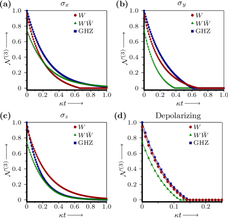
Figure 6.1: Simulation of decay of tripartite entanglement parameter negativity ${\cal N}^{(3)}$ of the GHZ state (blue squares), the W state (red circles) and the $W\bar{W}$ state (green triangles) under the action of (a) amplitude damping (Pauli $\sigma_{x}$) channel, (b) bit-phase flip (Pauli $\sigma_{y}$) channel (c) phase damping (Pauli $\sigma_{z}$) channel and (d) isotropic noise (depolarizing) channel. The $\kappa$ parameter denotes inverse of the decoherence time.

The analytical results of the Lindblad equation under the action of the different noise channels on tripartite entanglement are displayed in Fig. 6.1, where Figs. 6.1(a)-(d) show the decohering effects of the amplitude damping (Pauli $\sigma_{x}$) channel, the bit-phase flip (Pauli $\sigma_{y}$) channel, the phase damping (Pauli $\sigma_{z}$) channel and the depolarizing (isotropic noise) channel respectively, on the GHZ, W and ${\rm W\bar{W}}$ states. The simulation indicates that the W state is more robust against the phase-damping channel as compared to the GHZ state, while the reverse is true for the amplitude-damping channel. Both states decohere to nearly the same extent under the action of the bit-phase flip channel and the depolarizing channel. The ${\rm W\bar{W}}$ state decoheres more rapidly under the actions of the bit-phase flip channel and the depolarizing channel, as compared to the other GHZ and the W states. For short timescales its decoherence behavior mimics the W state under the action of the amplitude damping channel while for longer timescales it decoheres similar to the GHZ state. On the other hand, under the action of the phase-damping channel the ${\rm W\bar{W}}$ state initially decoheres faster than the GHZ state and later closely follows the GHZ decay behavior.

6.2.2 NMR system

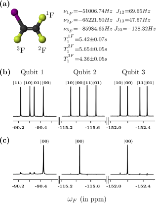
Figure 6.2: (a) Molecular structure of trifluoroiodoethylene molecule and tabulated system parameters with chemical shifts $\nu_{i}$ and scalar couplings J_ij (in Hz), and spin-lattice relaxation times $T_{1}$ and spin-spin relaxation times T₂ (in seconds). (b) NMR spectrum obtained after a $\pi/2$ readout pulse on the thermal equilibrium state. and (c) NMR spectrum of the pseudopure $|000\rangle$ state. The resonance lines of each qubit are labeled by the corresponding logical states of the other qubit.

We use the three ¹⁹F nuclear spins of the trifluoroiodoethylene (C₂F₃I) molecule to encode the three qubits. On an NMR spectrometer operating at 600 MHz, the fluorine spin resonates at a Larmor frequency of $\approx 564$ MHz. The molecular structure of the three-qubit system with tabulated system parameters and the NMR spectra of the qubits at thermal equilibrium and prepared in the pseudopure state $|000\rangle$ are shown in Figs. 6.2(a), (b), and (c), respectively. The Hamiltonian of a weakly-coupled three-spin system in a frame rotating at $\omega_{{\rm rf}}$ (the frequency of the electromagnetic field $B_{1}(t)$ applied to manipulate spins in a static magnetic field $B_{0}$) is given by [97]:

$${\cal H}=-\sum_{i=1}^{3}(\omega_{i}-\omega_{{\rm rf}})I_{iz}+\sum_{i<j,j=1}^{3}2\pi J_{ij}I_{iz}I_{jz}$$ (6.3)

where $I_{iz}$ is the spin angular momentum operator in the $z$ direction for ¹⁹F; the first term in the Hamiltonian denotes the Zeeman interaction between the fluorine spins and the static magnetic field $B_{0}$ with $\omega_{i}=2\pi\nu_{i}$ being the Larmor frequencies; the second term represents the spin-spin interaction with $J_{ij}$ being the scalar coupling constants. The three-qubit equilibrium density matrix (in the high temperature and high field approximations) is in a highly mixed state given by:

$$\rho_{eq} = \tfrac{1}{8}(I+\epsilon\ \Delta\rho_{eq})$$

$$\Delta\rho_{{\rm eq}} \propto \sum_{i=1}^{3}I_{iz}$$ (6.4)

with a thermal polarization $\epsilon\sim 10^{-5}$, $I$ being the $8\times 8$ identity operator and $\Delta\rho_{{\rm eq}}$ being the deviation part of the density matrix. The system was first initialized into the $|000\rangle$ pseudopure state using the spatial averaging technique [24], with the density operator given by

$$\rho_{000}=\frac{1-\epsilon}{8}I+\epsilon|000\rangle\langle 000|$$ (6.5)

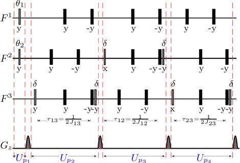
Figure 6.3: NMR pulse sequence used to prepare pseudopure state $\rho_{000}$ starting from thermal equilibrium.The pulses represented by black filled rectangles are of angle $\pi$. The other rf flip angles are set to $\theta_{1}=\frac{5\pi}{12}$, $\theta_{2}=\frac{\pi}{6}$ and $\delta=\frac{\pi}{4}$. The phase of each rf pulse is written below each pulse bar. The evolution interval $\tau_{ij}$ is set to a multiple of the scalar coupling strength ($J_{ij}$).

The specific sequence of rf pulses, $z$ gradient pulses and time evolution periods we used to prepare the pseudopure state $\rho_{000}$ starting from thermal equilibrium is shown in Fig. 6.3. All the rf pulses used in the pseudopure state preparation scheme were constructed using the Gradient Ascent Pulse Engineering (GRAPE) technique [25] and were designed to be robust against rf inhomogeneity, with an average fidelity of $\geq 0.99$. Wherever possible, two independent spin-selective rf pulses were combined using a specially crafted single GRAPE pulse; for instance the first two rf pulses to be applied before the first field gradient pulse, were combined into a single pulse specially crafted pulse ($U_{p_{1}}$ in Fig. 6.3), of duration $600\mu$s. The combined pulses $U_{p_{2}}$, $U_{p_{3}}$ and $U_{p_{4}}$ applied later in the sequence were of a total duration $\approx 20$ ms.

All experimental density matrices were reconstructed using a reduced tomographic protocol and by using maximum likelihood estimation [95, 59] as described in Chapter 2 with the set of operations $\{III,IIY,IYY,YII,XYX,XXY,$ $XXX\}$; $I$ is the identity (do-nothing operation) and $X(Y)$ denotes a single spin operator implemented by a spin-selective $\pi/2$ pulse. We constructed these spin-selective pulses for tomography using GRAPE, with the length of each pulse $\approx 600\mu$s. The experimentally created pseudopure state $|000\rangle$ was tomographed with a fidelity of 0.99 and the total time taken to prepare the state was $\approx 60$ ms. The fidelity of an experimental density matrix was computed using Eq. (2.32).

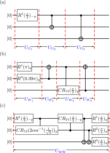
Figure 6.4: (Quantum circuit showing the sequence of implementation of the single-qubit local rotation gates (labeled by $R$), two-qubit controlled-rotation gates (labeled by $CR$) and controlled-NOT gates required to construct the (a) GHZ state (b) W state and (c) ${\rm W\bar{W}}$ state.

6.2.3 Construction of tripartite entangled states

Tripartite entanglement has been well characterized and it is known that the two different classes of tripartite entanglement, namely GHZ-class and W-class, are inequivalent. While both classes are maximally entangled, there are differences in the their type of entanglement: the W-class entanglement is more robust against particle loss than the GHZ-class (which becomes separable if one particle is lost) and it is also known that the W state has the maximum possible bipartite entanglement in its reduced two-qubit states [222]. The entanglement in the ${\rm W\bar{W}}$ state (which belongs to the GHZ-class of entanglement) shows a surprising result, that it is reconstructible from its reduced two-qubit states (similar to the W-class of states). We now turn to the construction of tripartite entangled states on the three-qubit NMR system. The quantum circuits to prepare the three qubits in a GHZ-type state, a W state and a ${\rm W\bar{W}}$ state are shown in Figs. 6.4 (a), (b) and (c), respectively. Several of the quantum gates in these circuits were optimized using the GRAPE algorithm and we were able to achieve a high gate fidelity and smaller pulse lengths.

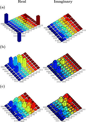
Figure 6.5: The real (left) and imaginary (right) parts of the experimentally tomographed (a) GHZ-type state, with a fidelity of $0.97$. (b) W state, with a fidelity of $0.96$ and (c) $W\bar{W}$ state with a fidelity of $0.94$. The rows and columns encode the computational basis in binary order from $|000\rangle$ to $|111\rangle$.

The GHZ-type $\frac{1}{\sqrt{2}}(|000\rangle-|111\rangle)$ state was prepared from the $|000\rangle$ pseudopure state by a sequence of three quantum gates (labeled as $U_{G_{1}},U_{G_{2}},U_{G_{3}}$ in Fig. 6.4(a)): first a selective rotation of $\left[\frac{\pi}{2}\right]_{-y}$ on the first qubit, followed by a CNOT₁₂ gate, and finally a CNOT₁₃ gate. The step-by-step sequential gate operation leads to:

$$|000\rangle \stackrel{{\scriptstyle{R^{1}{\left(\frac{\pi}{2}\right)_{-y}}}}}{{\longrightarrow}} \frac{1}{\sqrt{2}}\left(|000\rangle-|100\rangle\right)$$ (6.6)

$$\stackrel{{\scriptstyle\rm CNOT_{12}}}{{\longrightarrow}} \frac{1}{\sqrt{2}}\left(|000\rangle-|110\rangle\right)$$

$$\stackrel{{\scriptstyle\rm CNOT_{13}}}{{\longrightarrow}} \frac{1}{\sqrt{2}}\left(|000\rangle-|111\rangle\right)$$

All the pulses for the three gates used for GHZ state construction were designed using the GRAPE algorithm and had a fidelity $\geq$ 0.995. The GRAPE pulse duration corresponding to the gate $U_{G_{1}}$ is $600$ $\mu$s, while the $U_{G_{2}}$ and $U_{G_{3}}$ gates had pulse durations of $24$ ms. The GHZ-type state was prepared with a fidelity of 0.97. The W state was prepared from the initial $|000\rangle$ by a sequence of four unitary operations (labeled as $U_{W_{1}},U_{W_{2}},U_{W_{3}},U_{W_{4}}$ in Fig. 6.4(b) and the sequential gate operation leads to:

$$|000\rangle \stackrel{{\scriptstyle R^{1}\left({\pi}\right)_{y}}}{{\longrightarrow}} |100\rangle$$ (6.7)

$$\stackrel{{\scriptstyle\rm R^{2}\left({0.39\pi}\right)_{y}}}{{\longrightarrow}} \sqrt{\frac{2}{3}}|100\rangle+\frac{1}{\sqrt{3}}|110\rangle$$

$$\stackrel{{\scriptstyle\rm CNOT_{21}}}{{\longrightarrow}} \sqrt{\frac{2}{3}}|100\rangle+\frac{1}{\sqrt{3}}|010\rangle$$

$$\stackrel{{\scriptstyle\rm CR_{13}{\left(\frac{\pi}{2}\right)_{y}}}}{{\longrightarrow}} \frac{1}{\sqrt{3}}[|100\rangle+|101\rangle+|010\rangle]$$

$$\stackrel{{\scriptstyle\rm CNOT_{31}}}{{\longrightarrow}} \frac{1}{\sqrt{3}}[|100\rangle+|001\rangle+|010\rangle]$$

The different unitaries were individually optimized using GRAPE and the pulse duration for $U_{W_{1}}$, $U_{W_{2}}$, $U_{W_{3}}$, and $U_{W_{4}}$ turned out to be $600\mu$s, $24$ms, $16$ms, and $20$ms, respectively and the fidelity of the final state was estimated to be 0.94.

The ${\rm W\bar{W}}$ state was constructed by applying the following sequence of gate operations on the $|000\rangle$ state:

$$|000\rangle \stackrel{{\scriptstyle R^{1}\left(\frac{\pi}{3}\right)_{-y}}}{{\longrightarrow}} \frac{\sqrt{3}}{2}|000\rangle-\frac{1}{2}|100\rangle$$ (6.8)

$$\stackrel{{\scriptstyle\scriptstyle{\rm CR}_{12}\left(0.61\pi\right)_{y}}}{{\longrightarrow}} \frac{\sqrt{3}}{2}|000\rangle-\frac{1}{2\sqrt{3}}|100\rangle-\sqrt{\frac{1}{6}}|110\rangle$$

$$\stackrel{{\scriptstyle\scriptstyle{\rm CR}_{21}\left(\frac{\pi}{2}\right)_{-y}}}{{\longrightarrow}} \frac{1}{2}(\sqrt{3}|000\rangle-\frac{1}{\sqrt{3}}(|100\rangle+|110\rangle+$$

$$|010\rangle))$$

$$\stackrel{{\scriptstyle\rm CNOT_{13}}}{{\longrightarrow}} \frac{1}{2}(\sqrt{3}|000\rangle-\frac{1}{\sqrt{3}}(|101\rangle+|111\rangle+$$

$$|010\rangle))$$

$$\stackrel{{\scriptstyle\rm CNOT_{23}}}{{\longrightarrow}} \frac{1}{2}(\sqrt{3}|000\rangle-\frac{1}{\sqrt{3}}(|101\rangle+|110\rangle+$$

$$|011\rangle))$$

$$\stackrel{{\scriptstyle\rm R^{123}\left(\frac{\pi}{2}\right)_{y}}}{{\longrightarrow}} \frac{1}{\sqrt{6}}(|001\rangle+|010\rangle+|011\rangle+$$

$$|100\rangle+|101\rangle+|110\rangle)$$

The unitary operator for the entire preparation sequence (labeled $U_{W\bar{W}}$ in Fig. 6.4(c)) comprising a spin-selective rotation operator: two controlled-rotation gates, two controlled-NOT gates and one non-selective rotation by $\frac{\pi}{2}$ on all the three qubits, was created by a specially crafted single GRAPE pulse (of pulse length $48$ms) and applied to the initial state $|000\rangle$. The final state had a computed fidelity of 0.95.

6.2.4 Decay of tripartite entanglement

We next turn to the dynamics of tripartite entanglement under decoherence channels acting on the system. We studied the time evolution of the tripartite negativity ${\cal N}^{(3)}_{123}$ for the tripartite entangled states, as computed from the experimentally reconstructed density matrices at each time instant. The experimental results are depicted in Fig 6.6 (a), (b) and (c) for the GHZ state, the ${\rm W\bar{W}}$ state, and the W state, respectively. Of the three entangled states considered in this study, the GHZ and W states are maximally entangled and hence contain the most amount of tripartite negativity, while the ${\rm W\bar{W}}$ state is not maximally entangled and hence has a lower tripartite negativity value. The experimentally prepared GHZ state initially has a ${\cal N}^{(3)}_{123}$ of 0.96 (quite close to its theoretically expected value of 1.0). The GHZ state decays rapidly, with its negativity approaching zero in 0.55 s. The experimentally prepared ${\rm W\bar{W}}$ state initially has a ${\cal N}^{(3)}_{123}$ of 0.68 (close to its theoretically expected value of 0.74), with its negativity approaching zero at 0.67 s. The experimentally prepared W state initially has a ${\cal N}^{(3)}_{123}$ of 0.90 (quite close to its theoretically expected value of 0.94). The W state is quite long-lived, with its entanglement persisting up to 0.9 s. The tomographs of the experimentally reconstructed density matrices of the GHZ, W and ${\rm W\bar{W}}$ states at the time instances when the tripartite negativity parameter ${\cal N}^{(3)}_{123}$ approaches zero for each state, are displayed in Fig. 6.7.

Figure 6.6: Time dependence of the tripartite negativity ${\cal N}^{(3)}$ for the three-qubit system initially experimentally prepared in the (a) GHZ state (squares) (b) W state (circles) and (c) ${\rm W{\bar{W}}}$ state (triangles) (the superscript ${\rm exp}$ denotes “experimental data”). The fits are the calculated decay of negativity ${\cal N}^{(3)}$ of the GHZ state (solid line), the $W\bar{W}$ state (dashed line) and the W state (dotted-dashed line), under the action of the modeled NMR noise channel (the superscript ${\rm cal}$ denotes “calculated fit”). The W state is most robust against the NMR noise channel, whereas the GHZ state is most fragile.

We explored the noise channels acting on our three-qubit NMR entangled states which best fit our experimental data, by analytically solving a master equation in the Lindblad form, along the lines suggested in Reference [218]. The master equation is given by Eq. (6.1).

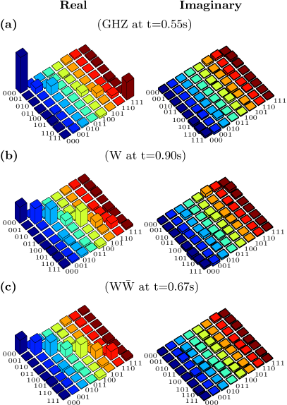
Figure 6.7: The real (left) and imaginary (right) parts of the experimentally tomographed density matrix of the state at the time instances when the tripartite negativity ${\cal N}^{(3)}_{123}$ approaches zero for the (a) GHZ state at $t=0.55$ s (b) W state at $t=0.90$ s and (c) ${\rm W\bar{W}}$ state at $t=0.67$ s. The rows and columns encode the computational basis in binary order, from $|000\rangle$ to $|111\rangle$.

We consider a decoherence model wherein a nuclear spin is acted on by two noise channels namely a phase damping channel (described by the T₂ relaxation in NMR) and a generalized amplitude damping channel (described by the T₁ relaxation in NMR) [67]. As the fluorine spins in our three-qubit system have widely differing chemical shifts, we assume that each qubit interacts independently with its own environment. The experimentally determined T₁ NMR relaxation rates are T${}_{1}^{1F}=5.42\pm 0.07$ s, T${}_{1}^{2F}=5.65\pm 0.05$ s and T${}_{1}^{3F}=4.36\pm 0.05$ s, respectively. The T₂ relaxation rates were experimentally measured by first rotating the spin magnetization into the transverse plane by a $90^{\circ}$ rf pulse followed by a delay and fitting the resulting magnetization decay. The experimentally determined T₂ NMR relaxation rates are T${}_{2}^{1F}=0.53\pm 0.02$s, T${}_{2}^{2F}=0.55\pm 0.02$ s, and T${}_{2}^{3F}=0.52\pm 0.02$ s, respectively. We solved the master equation (Eq. (6.1)) for the GHZ, W and ${\rm W\bar{W}}$ states with the Lindblad operators $L_{i,x}\equiv\sqrt{\frac{\kappa_{i,x}}{2}}\sigma^{(i)}_{x}$ and $L_{i,z}\equiv\sqrt{\frac{\kappa_{i,z}}{2}}\sigma^{(i)}_{z}$, where $\kappa_{i,x}=\frac{1}{T_{1}^{i}}$ and $\kappa_{i,z}=\frac{1}{T_{2}^{i}}$.

Under the simultaneous action of all the NMR noise channels, the GHZ state decoheres as:

$$\rho_{GHZ}=\left(\begin{array}[]{cccccccc}\alpha_{1}&0&0&0&0&0&0&\beta_{1}\\ 0&\alpha_{2}&0&0&0&0&\beta_{2}&0\\ 0&0&\alpha_{3}&0&0&\beta_{3}&0&0\\ 0&0&0&\alpha_{4}&\beta_{4}&0&0&0\\ 0&0&0&\beta_{4}&\alpha_{4}&0&0&0\\ 0&0&\beta_{3}&0&0&\alpha_{3}&0&0\\ 0&\beta_{2}&0&0&0&0&\alpha_{2}&0\\ \beta_{1}&0&0&0&0&0&0&\alpha_{1}\\ \end{array}\right)$$ (6.9)

where

$$\alpha_{1} = \frac{1}{8}(1+e^{-(\kappa_{x,1}+\kappa_{x,2})t}+e^{-(\kappa_{x,1}+\kappa_{x,3})t}+e^{-(\kappa_{x,2}+\kappa_{x,3})t})$$

$$\alpha_{2} = \frac{1}{8}(1+e^{-(\kappa_{x,1}+\kappa_{x,2})t}-e^{-(\kappa_{x,1}+\kappa_{x,3})t}-e^{-(\kappa_{x,2}+\kappa_{x,3})t})$$

$$\alpha_{3} = \frac{1}{8}(1-e^{-(\kappa_{x,1}+\kappa_{x,2})t}+e^{-(\kappa_{x,1}+\kappa_{x,3})t}-e^{-(\kappa_{x,2}+\kappa_{x,3})t})$$

$$\alpha_{4} = \frac{1}{8}(1-e^{-(\kappa_{x,1}+\kappa_{x,2})t}-e^{-(\kappa_{x,1}+\kappa_{x,3})t}+e^{-(\kappa_{x,2}+\kappa_{x,3})t})$$

$$\beta_{1} = \frac{1}{8}(e^{-(\kappa_{1,x}+\kappa_{2,x}+\kappa_{3,x}+\kappa_{1,z}+\kappa_{2,z}+\kappa_{3,z})t}$$

$$\quad(e^{\kappa_{1,x}t}+e^{\kappa_{2,x}t}+e^{\kappa_{3,x}t}+e^{(\kappa_{1,x}+\kappa_{2,x}+\kappa_{3,x})t})$$

$$\beta_{2} = \frac{1}{8}(e^{-(\kappa_{1,x}+\kappa_{2,x}+\kappa_{3,x}+\kappa_{1,z}+\kappa_{2,z}+\kappa_{3,z})t}$$

$$\quad(-e^{\kappa_{1,x}t}-e^{\kappa_{2,x}t}+e^{\kappa_{3,x}t}+e^{(\kappa_{1,x}+\kappa_{2,x}+\kappa_{3,x})t})$$

$$\beta_{3} = \frac{1}{8}(e^{-(\kappa_{1,x}+\kappa_{2,x}+\kappa_{3,x}+\kappa_{1,z}+\kappa_{2,z}+\kappa_{3,z})t}$$

$$(-e^{\kappa_{1,x}t}+e^{\kappa_{2,x}t}-e^{\kappa_{3,x}t}+e^{(\kappa_{1,x}+\kappa_{2,x}+\kappa_{3,x})t})$$

$$\beta_{4} = \frac{1}{8}(e^{-(\kappa_{1,x}+\kappa_{2,x}+\kappa_{3,x}+\kappa_{1,z}+\kappa_{2,z}+\kappa_{3,z})t}$$

$$\quad(e^{\kappa_{1,x}t}-e^{\kappa_{2,x}t}-e^{\kappa_{3,x}t}+e^{(\kappa_{1,x}+\kappa_{2,x}+\kappa_{3,x})t})$$

Under the simultaneous action of all the NMR noise channels, the W state decoheres as:

$$\rho_{W}=\left(\begin{array}[]{cccccccc}\alpha_{1}&0&0&\beta_{1}&0&\beta_{5}&\beta_{1}&0\\ 0&\alpha_{2}&\beta_{2}&0&\beta_{6}&0&0&\beta_{10}\\ 0&\beta_{2}&\alpha_{3}&0&\beta_{11}&0&0&\beta_{7}\\ \beta_{1}&0&0&\alpha_{4}&0&\beta_{12}&\beta_{8}&0\\ 0&\beta_{6}&\beta_{11}&0&\alpha_{5}&0&0&\beta_{3}\\ \beta_{5}&0&0&\beta_{12}&0&\alpha_{6}&\beta_{4}&0\\ \beta_{1}&0&0&\beta_{8}&0&\beta_{4}&\alpha_{7}&0\\ 0&\beta_{10}&\beta_{7}&0&\beta_{3}&0&0&\alpha_{8}\\ \end{array}\right)\\$$

Where

$$\alpha_{1} = \frac{1}{8}-\frac{1}{24}e^{-(\kappa_{x,1}+\kappa_{x,2}+\kappa_{x,3})t}(3+e^{\kappa_{x,1}t}+e^{\kappa_{x,2}t}-$$

$$e^{(\kappa_{x,1}+\kappa_{x,2})t}+e^{\kappa_{x,3}t}-e^{(\kappa_{x,1}+\kappa_{x,3})t}-e^{(\kappa_{x,2}+\kappa_{x,3})t})$$

$$\alpha_{2} = \frac{1}{8}+\frac{1}{24}e^{-(\kappa_{x,1}+\kappa_{x,2}+\kappa_{x,3})t}(3+e^{\kappa_{x,1}t}+e^{\kappa_{x,2}t}-$$

$$e^{(\kappa_{x,1}+\kappa_{x,2})t}-e^{\kappa_{x,3}t}+e^{(\kappa_{x,1}+\kappa_{x,3})t}+e^{(\kappa_{x,2}+\kappa_{x,3})t})$$

$$\alpha_{3} = \frac{1}{8}+\frac{1}{24}e^{-(\kappa_{x,1}+\kappa_{x,2}+\kappa_{x,3})t}(3+e^{\kappa_{x,1}t}-e^{\kappa_{x,2}t}$$

$$+e^{(\kappa_{x,1}+\kappa_{x,2})t}+e^{\kappa_{x,3}t}-e^{(\kappa_{x,1}+\kappa_{x,3})t}+e^{(\kappa_{x,2}+\kappa_{x,3})t})$$

$$\alpha_{4} = \frac{1}{8}-\frac{1}{24}e^{-(\kappa_{x,1}+\kappa_{x,2}+\kappa_{x,3})t}(3+e^{\kappa_{x,1}t}-e^{\kappa_{x,2}t}$$

$$+e^{(\kappa_{x,1}+\kappa_{x,2})t}-e^{\kappa_{x,3}t}+e^{(\kappa_{x,1}+\kappa_{x,3})t}-e^{(\kappa_{x,2}+\kappa_{x,3})t})$$

$$\alpha_{5} = \frac{1}{8}+\frac{1}{24}e^{-(\kappa_{x,1}+\kappa_{x,2}+\kappa_{x,3})t}(3-e^{\kappa_{x,1}t}+e^{\kappa_{x,2}t}$$

$$+e^{(\kappa_{x,1}+\kappa_{x,2})t}+e^{\kappa_{x,3}t}+e^{(\kappa_{x,1}+\kappa_{x,3})t}-e^{(\kappa_{x,2}+\kappa_{x,3})t})$$

$$\alpha_{6} = \frac{1}{8}+\frac{1}{24}e^{-(\kappa_{x,1}+\kappa_{x,2}+\kappa_{x,3})t}(-3+e^{\kappa_{x,1}t}-e^{\kappa_{x,2}t}$$

$$-e^{(\kappa_{x,1}+\kappa_{x,2})t}+e^{\kappa_{x,3}t}+e^{(\kappa_{x,1}+\kappa_{x,3})t}-e^{(\kappa_{x,2}+\kappa_{x,3})t})$$

$$\alpha_{7} = \frac{1}{8}+\frac{1}{24}e^{-(\kappa_{x,1}+\kappa_{x,2}+\kappa_{x,3})t}(-3+e^{\kappa_{x,1}t}+e^{\kappa_{x,2}t}$$

$$+e^{(\kappa_{x,1}+\kappa_{x,2})t}-e^{\kappa_{x,3}t}-e^{(\kappa_{x,1}+\kappa_{x,3})t}-e^{(\kappa_{x,2}+\kappa_{x,3})t})$$

$$\alpha_{8} = \frac{1}{8}-\frac{1}{24}e^{-(\kappa_{x,1}+\kappa_{x,2}+\kappa_{x,3})t}(-3+e^{\kappa_{x,1}t}+e^{\kappa_{x,2}t}$$

$$+e^{(\kappa_{x,1}+\kappa_{x,2})t}+e^{\kappa_{x,3}t}+e^{(\kappa_{x,1}+\kappa_{x,3})t}+e^{(\kappa_{x,2}+\kappa_{x,3})t})$$

$$\beta_{1} = \frac{1}{12}(e^{-(\kappa_{x,1}+\kappa_{x,2}+\kappa_{x,3}+\kappa_{z,2}+\kappa_{z,3})t}$$

$$(1+e^{(\kappa_{x,1})t})(-1+e^{(\kappa_{x,2}+\kappa_{x,3})t}))$$

$$\beta_{2} = \frac{1}{12}(e^{-(\kappa_{x,1}+\kappa_{x,2}+\kappa_{x,3}+\kappa_{z,2}+\kappa_{z,3})t}$$

$$(1+e^{(\kappa_{x,1})t})(1+e^{(\kappa_{x,2}+\kappa_{x,3})t}))$$

$$\beta_{3} = \frac{1}{12}(e^{-(\kappa_{x,1}+\kappa_{x,2}+\kappa_{x,3}+\kappa_{z,2}+\kappa_{z,3})t}$$

$$(-1+e^{(\kappa_{x,1})t})(-1+e^{(\kappa_{x,2}+\kappa_{x,3})t}))$$

$$\beta_{4} = \frac{1}{12}(e^{-(\kappa_{x,1}+\kappa_{x,2}+\kappa_{x,3}+\kappa_{z,2}+\kappa_{z,3})t}$$

$$(-1+e^{(\kappa_{x,1})t})(1+e^{(\kappa_{x,2}+\kappa_{x,3})t}))$$

$$\beta_{5} = \frac{1}{12}(e^{-(\kappa_{x,1}+\kappa_{x,2}+\kappa_{x,3}+\kappa_{z,1}+\kappa_{z,3})t}$$

$$(1+e^{(\kappa_{x,2})t})(-1+e^{(\kappa_{x,1}+\kappa_{x,3})t}))$$

$$\beta_{6} = \frac{1}{12}(e^{-(\kappa_{x,1}+\kappa_{x,2}+\kappa_{x,3}+\kappa_{z,1}+\kappa_{z,3})t}$$

$$(1+e^{(\kappa_{x,2})t})(1+e^{(\kappa_{x,1}+\kappa_{x,3})t}))$$

$$\beta_{7} = \frac{1}{12}(e^{-(\kappa_{x,1}+\kappa_{x,2}+\kappa_{x,3}+\kappa_{z,1}+\kappa_{z,3})t}$$

$$(-1+e^{(\kappa_{x,2})t})(-1+e^{(\kappa_{x,1}+\kappa_{x,3})t}))$$

$$\beta_{8} = \frac{1}{12}(e^{-(\kappa_{x,1}+\kappa_{x,2}+\kappa_{x,3}+\kappa_{z,1}+\kappa_{z,3})t}$$

$$(-1+e^{(\kappa_{x,2})t})(1+e^{(\kappa_{x,1}+\kappa_{x,3})t}))$$

$$\beta_{9} = \frac{1}{12}(e^{-(\kappa_{x,1}+\kappa_{x,2}+\kappa_{x,3}+\kappa_{z,1}+\kappa_{z,2})t}$$

$$(-1+e^{(\kappa_{x,1}+\kappa_{x,2})t})(1+e^{(\kappa_{x,3})t}))$$

$$\beta_{10} = \frac{1}{12}(e^{-(\kappa_{x,1}+\kappa_{x,2}+\kappa_{x,3}+\kappa_{z,1}+\kappa_{z,2})t}$$

$$(-1+e^{(\kappa_{x,1}+\kappa_{x,2})t})(-1+e^{(\kappa_{x,3})t}))$$

$$\beta_{11} = \frac{1}{12}(e^{-(\kappa_{x,1}+\kappa_{x,2}+\kappa_{x,3}+\kappa_{z,1}+\kappa_{z,2})t}$$

$$(1+e^{(\kappa_{x,1}+\kappa_{x,2})t})(1+e^{(\kappa_{x,3})t}))$$

$$\beta_{12} = \frac{1}{12}(e^{-(\kappa_{x,1}+\kappa_{x,2}+\kappa_{x,3}+\kappa_{z,1}+\kappa_{z,2})t}$$ (6.14)

$$(1+e^{(\kappa_{x,1}+\kappa_{x,2})t})(-1+e^{(\kappa_{x,3})t}))$$

Under the simultaneous action of all the NMR noise channels, the ${\rm W\bar{W}}$ state decoheres as:

$$\rho_{{\rm W\bar{W}}}=\left(\begin{array}[]{cccccccc}\alpha_{1}&\beta_{1}&\beta_{2}&\beta_{3}&\beta_{4}&\beta_{5}&\beta_{6}&\beta_{7}\\ \beta_{1}&\alpha_{2}&\beta_{8}&\beta_{9}&\beta_{10}&\beta_{11}&\beta_{12}&\beta_{13}\\ \beta_{2}&\beta_{8}&\alpha_{3}&\beta_{14}&\beta_{15}&\beta_{16}&\beta_{11}&\beta_{5}\\ \beta_{3}&\beta_{9}&\beta_{14}&\alpha_{4}&\beta_{17}&\beta_{15}&\beta_{10}&\beta_{4}\\ \beta_{4}&\beta_{10}&\beta_{15}&\beta_{17}&\alpha_{4}&\beta_{15}&\beta_{9}&\beta_{18}\\ \beta_{5}&\beta_{11}&\beta_{16}&\beta_{15}&\beta_{15}&\alpha_{3}&\beta_{8}&\beta_{2}\\ \beta_{6}&\beta_{12}&\beta_{11}&\beta_{10}&\beta_{9}&\beta_{8}&\alpha_{2}&\beta_{1}\\ \beta_{7}&\beta_{13}&\beta_{5}&\beta_{4}&\beta_{18}&\beta_{2}&\beta_{1}&\alpha_{1}\\ \end{array}\right)$$ (6.15)

where

$$\alpha_{1} = \frac{1}{24}(3-e^{-(\kappa_{x,1}+\kappa_{x,2})t}-e^{-(\kappa_{x,1}+\kappa_{x,3})t}$$

$$-e^{-(\kappa_{x,2}+\kappa_{x,3})t})$$

$$\alpha_{2} = \frac{1}{24}(3-e^{-(\kappa_{x,1}+\kappa_{x,2})t}+e^{-(\kappa_{x,1}+\kappa_{x,3})t}$$

$$+e^{-(\kappa_{x,2}+\kappa_{x,3})t})$$

$$\alpha_{3} = \frac{1}{24}(3+e^{-(\kappa_{x,1}+\kappa_{x,2})t}-e^{-(\kappa_{x,1}+\kappa_{x,3})t}$$

$$+e^{-(\kappa_{x,2}+\kappa_{x,3})t})$$

$$\alpha_{4} = \frac{1}{24}(3+e^{-(\kappa_{x,1}+\kappa_{x,2})t}+e^{-(\kappa_{x,1}+\kappa_{x,3})t}$$

$$-e^{-(\kappa_{x,2}+\kappa_{x,3})t})$$

$$\beta_{1} = \frac{1}{12}e^{-(\kappa_{x,1}+\kappa_{x,2}+2\kappa_{z,3})t}$$

$$(e^{(\kappa_{x,1}+\kappa_{x,2}+\kappa_{z,3})t}-e^{\kappa_{z,3}t})$$

$$\beta_{2} = \frac{1}{12}e^{-(\kappa_{x,1}+\kappa_{x,3}+2\kappa_{z,2})t}$$

$$(e^{(\kappa_{x,1}+\kappa_{x,3}+\kappa_{z,2})t}-e^{\kappa_{z,2}t})$$

$$\beta_{3} = \frac{1}{12}e^{-(\kappa_{x,2}+\kappa_{x,3}+2(\kappa_{z,2}+\kappa_{z,3}))t}$$

$$(e^{(\kappa_{x,2}+\kappa_{x,3}+\kappa_{z,2}+\kappa_{z,3})t}-e^{(\kappa_{z,2}+\kappa_{z,3})t})$$

$$\beta_{4} = \frac{1}{12}e^{-(\kappa_{x,2}+\kappa_{x,3}+2\kappa_{z,1})t}$$

$$(-e^{\kappa_{z,1}t}+e^{(\kappa_{x,2}+\kappa_{x,3}+\kappa_{z,1})t})$$

$$\beta_{5} = \frac{1}{12}e^{-(\kappa_{x,1}+\kappa_{x,3}+2(\kappa_{z,1}+\kappa_{z,3}))t}$$

$$(-e^{(\kappa_{z,1}+\kappa_{z,3})t}+e^{(\kappa_{x,1}+\kappa_{x,3}+\kappa_{z,1}+\kappa_{z,3})t})$$

$$\beta_{6} = \frac{1}{12}e^{-(\kappa_{x,1}+\kappa_{x,2}+2(\kappa_{z,1}+\kappa_{z,2}))t}$$

$$(-e^{(\kappa_{z,1}+\kappa_{z,2})t}+e^{(\kappa_{x,1}+\kappa_{x,2}+\kappa_{z,1}+\kappa_{z,2})t})$$

$$\beta_{7} = -\frac{1}{24}e^{-(\kappa_{x,1}+\kappa_{x,2}+\kappa_{x,3}+\kappa_{z,1}+\kappa_{z,2}+\kappa_{z,3})t}$$

$$(e^{\kappa_{x,1}t}+e^{\kappa_{x,2}t}+e^{\kappa_{x,3}t}-3e^{(\kappa_{x,1}+\kappa_{x,2}+\kappa_{x,3})t})$$

$$\beta_{8} = \frac{1}{12}e^{-(\kappa_{x,2}+\kappa_{x,3}+2(\kappa_{z,2}+\kappa_{z,3}))t}$$

$$(e^{(\kappa_{z,2}+\kappa_{z,3})t}+e^{(\kappa_{x,2}+\kappa_{x,3}+\kappa_{z,2}+\kappa_{z,3})t})$$

$$\beta_{9} = \frac{1}{12}e^{-(\kappa_{x,1}+\kappa_{x,3}+2\kappa_{z,2})t}$$

$$(e^{\kappa_{z,2}t}+e^{(\kappa_{x,1}+\kappa_{x,3}+\kappa_{z,2})t})$$

$$\beta_{10} = \frac{1}{12}e^{-(\kappa_{x,1}+\kappa_{x,3}+2(\kappa_{z,1}+\kappa_{z,3}))t}$$

$$(e^{(\kappa_{z,1}+\kappa_{z,3})t}+e^{(\kappa_{x,1}+\kappa_{x,3}+\kappa_{z,1}+\kappa_{z,3})t})$$

$$\beta_{11} = \frac{1}{12}e^{-(\kappa_{x,2}+\kappa_{x,3}+2\kappa_{z,1})t}(e^{\kappa_{z,1}t}+e^{(\kappa_{x,2}+\kappa_{x,3}+\kappa_{z,1})t})$$

$$\beta_{12} = \frac{1}{24}e^{-(\kappa_{x,1}+\kappa_{x,2}+\kappa_{x,3}+\kappa_{z,1}+\kappa_{z,2}+\kappa_{z,3})t}$$

$$(e^{\kappa_{x,1}t}+e^{\kappa_{x,2}t}-e^{\kappa_{x,3}t}+3e^{(\kappa_{x,1}+\kappa_{x,2}+\kappa_{x,3})t})$$

$$\beta_{13} = \frac{1}{12}e^{-(\kappa_{x,1}+\kappa_{x,2}+2(\kappa_{z,1}+\kappa_{z,2}))t}$$

$$(-e^{(\kappa_{z,1}+\kappa_{z,2})t}+e^{(\kappa_{x,1}+\kappa_{x,2}+\kappa_{z,1}+\kappa_{z,2})t})$$

$$\beta_{14} = \frac{1}{12}e^{-(\kappa_{x,1}+\kappa_{x,2}+2\kappa_{z,3})t}$$

$$(e^{\kappa_{z,3}t}+e^{(\kappa_{x,1}+\kappa_{x,2}+\kappa_{z,3})t})$$

$$\beta_{15} = \frac{1}{12}e^{-(\kappa_{x,1}+\kappa_{x,2}+2(\kappa_{z,1}+\kappa_{z,2}))t}$$

$$(e^{(\kappa_{z,1}+\kappa_{z,2})t}+e^{(\kappa_{x,1}+\kappa_{x,2}+\kappa_{z,1}+\kappa_{z,2})t})$$

$$\beta_{16} = \frac{1}{24}e^{-(\kappa_{x,1}+\kappa_{x,2}+\kappa_{x,3}+\kappa_{z,1}+\kappa_{z,2}+\kappa_{z,3})t}$$

$$(e^{\kappa_{x,1}t}-e^{\kappa_{x,2}t}+e^{\kappa_{x,3}t}+3e^{(\kappa_{x,1}+\kappa_{x,2}+\kappa_{x,3})t})$$

$$\beta_{17} = \frac{1}{24}e^{-(\kappa_{x,1}+\kappa_{x,2}+\kappa_{x,3}+\kappa_{z,1}+\kappa_{z,2}+\kappa_{z,3})t}$$

$$(-e^{\kappa_{x,1}t}+e^{\kappa_{x,2}t}+e^{\kappa_{x,3}t}+3e^{(\kappa_{x,1}+\kappa_{x,2}+\kappa_{x,3})t})$$

$$\beta_{18} = \frac{1}{12}e^{-(\kappa_{x,2}+\kappa_{x,3}+2(\kappa_{z,2}+\kappa_{z,3}))t}$$ (6.19)

$$(e^{(\kappa_{z,2}+\kappa_{z,3})t}+e^{(\kappa_{x,2}+\kappa_{x,3}+\kappa_{z,2}+\kappa_{z,3})t})$$

With this model, the GHZ state decays at the rate $\gamma^{al}_{GHZ}=6.33\pm 0.06s^{-1}$, and its entanglement approaches zero in 0.53 s. The $W\bar{W}$ state decays at the rate $\gamma^{al}_{W\bar{W}}=5.90\pm 0.10s^{-1}$, and its entanglement approaches zero in 0.50 s. The $W$ state decays at the rate $\gamma^{al}_{W}=4.84\pm 0.07s^{-1}$, and its entanglement approaches zero in 0.62 s. Solving the master equation (Eq. (6.1)) ensures that the off-diagonal elements of the corresponding $\rho$ matrices satisfy a set of coupled equations, from which the explicit values of $\alpha$s and $\beta$s can be computed. The equations are solved in the high-temperature limit. For an ensemble of NMR spins at room temperature this implies that the energy $E<<k_{B}T$ where $k_{B}$ is the Boltzmann constant and $T$ refers to the temperature, ensuring a Boltzmann distribution of spin populations at thermal equilibrium. The results of the analytical calculation and the experimental data match well, as shown in Fig. 6.6.

6.3 Protecting three-qubit entanglement via dynamical decoupling

As the tripartite entangled states under investigation are robust against noise to varying extents, we wanted to discover if either the amount of entanglement in these states could be protected or their entanglement could be preserved for longer times, using dynamical decoupling (DD) protection schemes. While DD sequences are effective in decoupling system-environment interactions, often errors in their implementation arise either due to errors in the pulses or errors due to off-resonant driving [54].

Figure 6.8: NMR pulse sequence corresponding to (a) XY-16(s) and (b) KDD_xy DD schemes (the superscript 2 implies that the set of pulses inside the bracket is applied twice, to form one cycle of the DD scheme). The pulses represented by black filled rectangles (in both schemes) are of angle $\pi$, and are applied simultaneously on all three qubits (denoted by $F^{i},i=1,2,3$). The angle below each pulse denotes the phase with which it is applied. Each DD cycle is repeated $N$ times, with $N$ large to achieve good system-bath decoupling.

Two approaches have been used to design robust DD sequences which are impervious to pulse imperfections: the first approach replaces the $\pi$ rotation pulses with composite pulses inside the DD sequence, while the second approach focuses on optimizing phases of the pulses in the DD sequence. In this work, we use DD sequences that use pulses with phases applied along different rotation axes: the XY-16(s) and the Knill Dynamical Decoupling (KDD) schemes [69]. In conventional DD schemes the $\pi$ pulses are applied along one axis (typically $x$) and as a consequence, only the coherence along that axis is well protected. The XY family of DD schemes applies pulses along two perpendicular ($x,y$) axes, which protects coherence equally along both these axes [223]. The XY-16(s) sequence is constructed by combining an XY-8(s) cycle with its phase-shifted copy, where the (s) denotes the “symmetric” version i.e. the cycle is time-symmetric with respect to its center. The XY-8 cycle is itself created by combining a basic XY-4 cycle with its time-reversed copy. One full unit cycle of the XY-16(s) sequence comprises sixteen $\pi$ pulses interspersed with free evolution time periods, and each cycle is repeated $N$ times for better decoupling. The KDD sequence has additional phases which further symmetrize pulses in the $x-y$ plane and compensate for pulse errors; each $\pi$ pulse in a basic XY DD sequence is replaced by five $\pi$ pulses, each of a different phase [224, 68]:

$${\rm KDD}_{\phi}\equiv(\pi)_{\frac{\pi}{6}+\phi}-(\pi)_{\phi}-(\pi)_{\frac{\pi}{2}+\phi}-(\pi)_{\phi}-(\pi)_{\frac{\pi}{6}+\phi}$$ (6.20)

where $\phi$ denotes the phase of the pulse; we set $\phi=0$ in our experiments. The KDD_ϕ sequence of five pulses given in Eq. (6.20) protects coherence along only one axis. To protect coherences along both the $(x,y)$ axes, we use the KDD_xy sequence, which combines two basic five-pulse blocks shifted in phase by $\pi/2$ i.e $[{\rm KDD}_{\phi}-{\rm KDD}_{\phi+\pi/2}]$. One unit cycle of the KDD_xy sequence contains two of these pulse-blocks shifted in phase, for a total of twenty $\pi$ pulses. The XY-16(s) and KDD_xy DD sequences are given in Figs. 6.8(a) and (b) respectively, where the black filled rectangles represent $\pi$ pulses on all three qubits and $\tau$ ($\tau_{k}$) indicates a free evolution time period. We note here that the chemical shifts of the three fluorine qubits in our particular molecule cover a very large frequency bandwidth, making it difficult to implement an accurate non-selective pulse simultaneously on all the qubits. To circumvent this problem, we crafted a special excitation pulse of duration $\approx 400\mu$s consisting of a set of three Gaussian shaped pulses that are applied at different spin frequency offsets and are frequency modulated to achieve simultaneous excitation [139].

Figs.6.9(a),(b) and (c) show the results of protecting the GHZ, W and ${\rm W\bar{W}}$ states respectively, using the XY-16(s) and the KDD_xy DD sequences.

GHZ state protection: The XY-16(s) protection scheme was implemented on the GHZ state with an inter-pulse delay of $\tau=0.25$ ms and one run of the sequence took $10.40$ ms (including the length of the sixteen $\pi$ pulses). The value of the negativity ${\cal N}^{3}_{123}$ remained close to 0.80 and 0.52 for up to $80$ms and $240$ ms respectively when XY-16 protection was applied, while for the unprotected state the state fidelity is quite low and ${\cal N}^{3}_{123}$ decayed to a low value of 0.58 and 0.09 at $80$ms and $240$ ms, respectively (Fig. 6.9(a)). The KDD_xy protection scheme on this state was implemented with an inter-pulse delay $\tau_{k}=0.20$ ms and one run of the sequence took $12$ ms (including the length of the twenty $\pi$ pulses). The value of the negativity ${\cal N}^{3}_{123}$ remained close to 0.80 and 0.72 for up to $140$ms and $240$ ms when KDD_xy protection was applied (Fig. 6.9(a)).

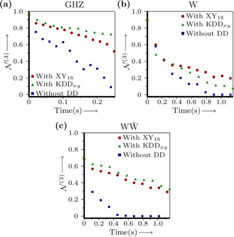
Figure 6.9: Plot of the tripartite negativity (${\cal N}^{(3)}_{123}$) with time, computed for the (a) GHZ-type state, (b) W state and (c) $W\bar{W}$ state. The negativity was computed for each state without applying any protection and after applying the XY-16(s) and KDD_xy dynamical decoupling sequences.Note that the time scale for part (a) is different from (b) and (c)

W state protection: The XY-16(s) protection scheme was implemented on the W state with an inter-pulse delay $\tau=3.12$ ms and one run of the sequence took $56.40$ ms (including the length of the sixteen $\pi$ pulses). The value of the negativity ${\cal N}^{3}_{123}$ remained close to 0.30 for up to $0.68$ s when XY-16 protection was applied, whereas ${\cal N}^{3}_{123}$ reduced to 0.1 at $0.68$ s when no state protection is applied (Fig. 6.9(b)). The KDD_xy protection scheme was implemented on the W state with an inter-pulse delay $\tau_{k}=2.5$ ms and one run of the sequence took $58$ ms (including the length of the twenty $\pi$ pulses). The value of the negativity ${\cal N}^{3}_{123}$ remained close to 0.21 for upto $0.70$ s when KDD_xy protection was applied (Fig. 6.9(b)).

${\rm W\bar{W}}$ state protection: The XY-16(s) protection sequence was implemented on the ${\rm W\bar{W}}$ state with an inter-pulse delay of $\tau=3.12$ ms and one run of the sequence took $56.40$ ms (including the length of the sixteen $\pi$ pulses). The value of the negativity ${\cal N}^{3}_{123}$ remained close to 0.5 for upto $0.45$ s when XY-16(s) protection was applied, whereas ${\cal N}^{3}_{123}$ reduced almost to zero ($\approx 0.02$) at $0.45$ s when no protection was applied (Fig. 6.9(c)). The KDD_xy protection sequence was applied with an inter-pulse delay of $\tau_{k}=2.5$ ms and one run of the sequence took $58$ ms (including the length of the twenty $\pi$ pulses). The value of the negativity ${\cal N}^{3}_{123}$ remained close to 0.52 for upto $0.46$ s when KDD_xy protection was applied (Fig. 6.9(c)).

The results of UDD-type of protection summarized above demonstrate that state protection worked to varying degrees and protected the entanglement of the tripartite entangled states to different extents, depending on the type of state to be protected. The GHZ state showed maximum protection and the ${\rm W\bar{W}}$ state also showed a significant amount of protection, while the W state showed a marginal improvement under protection. We note here that the lifetime of the GHZ state is not significantly enhanced by using DD state protection; what is noteworthy is that state fidelity remains high (close to 0.8) under DD protection, whereas the state quickly gets disentangled (fidelity drops to 0.4) when no protection is applied. This implies that under DD protection, there is no leakage from the state to other states in the Hilbert space of the three qubits.

6.4 Conclusions

An experimental study of the dynamics of tripartite entangled states in a three-qubit NMR system was undertaken. The results are relevant in the context of other studies which showed that different entangled states exhibit varying degrees of robustness against diverse noise channels. The W state was found to be the most robust against the decoherence channel acting on the three NMR qubits, the GHZ state was the most fragile and decayed very quickly, while the ${\rm W\bar{W}}$ state was more robust than the GHZ state but less robust than the W state. For entanglement protection dynamical decoupling sequences were implemented on these states. Both DD schemes were able to achieve a good degree of entanglement protection. The GHZ state was dramatically protected, with its entanglement persisting for nearly double the time. The W state showed a marginal improvement, which was to be expected since these DD schemes are designed to protect mainly against dephasing noise, and the experimental results indicated that the W state is already robust against this type of decohering channel. Interestingly, although the $\rm W{\bar{W}}$ state belongs to the GHZ entanglement-class, our experiments revealed that its entanglement persists for a longer time than the GHZ state, while the DD schemes are able to preserve its entanglement to a reasonable extent. The decoherence characteristics of the ${\rm W\bar{W}}$ state hence suggest a way of protecting fragile GHZ-type states against noise by transforming the type of entanglement (since a GHZ-class state can be transformed via local operations to a ${\rm W\bar{W}}$ state). These aspects of the entanglement dynamics of the ${\rm W{\bar{W}}}$ state require more detailed studies for a better understanding.

This work has provided new insights into the way entanglement behaves under decoherence and can be protected from the same. This kind of protection strategies will provide a benchmark for extension to higher qubit systems and to the study of different classes of entangled states. The ${\rm W{\bar{W}}}$ state is in the GHZ class, however its dynamics under decoherence resembles the W state, thereby providing it a certain amount of immunity under dephasing. This aspect, coupled with the protection schemes, can lead to new ways of entanglement protection.

Chapter 7 Summary and future outlook

The first project in this thesis focused on the reconstruction of a density matrix. The density matrix which was reconstructed using the standard quantum state tomography (QST) method had a few negative eigenvalues, which makes it an invalid density matrix. The maximum likelihood (ML) estimation method estimates the quantum state density matrix by determining the parameters that are most likely to match the experimentally generated data. The evaluation starts with initial parameters based on a priori knowledge of experimentally reconstructed density matrix. By putting a constraint at every stage of the estimation process, the density matrix was obtained to be positive and normalized. The standard QST method led to negative eigenvalues in the reconstructed density matrix and hence an overestimation of the entanglement parameter quantifying the residual entanglement in the state. The ML estimation method on the other hand, by virtue of its leading to a physical density matrix reconstruction every time, gives us a true measure of residual entanglement, and hence can be used to quantitatively study the decoherence of multiqubit entanglement. In this thesis ML estimation method is applied on two- and three-qubit systems. The ML estimation can extended further for higher qubit, but this kind of characterization of quantum states becomes too costly as the number of qubits increase. To solve this problem one can look for the use of graphics processing units (GPUs) by incorporating them in the optimization process, as it is recently used for speedup in quantum optimal control [225].

The later part of the thesis focused on mitigating the unwanted effects of system-environment interaction. The efficacy of different system-environment decoupling strategies were explored experimentally. These strategies were built depending on our knowledge about the system-environment interactions and the state to be preserved.

The first situation considered was one where the state of the system was known, and the system-environment interaction was unknown. The state was protected against evolution using the super-Zeno scheme. The next situation considered was one where only the subspace to which the state belongs was known and an arbitrary state belonging to known subspace was protected using the nested Uhrig dynamical decoupling (NUDD) scheme. The advantage of the NUDD schemes lies in the fact that one is sure that some amount of state protection will always be achieved.

Next, a system was considered whose state as well as interaction with the environment is known. A Bell-diagonal (BD) state was experimentally prepared on a two-qubit system. The noise model considered was that of each qubit was mainly affected by an independent phase damping channel, and quantum discord of the system was observed. Quantum discord remained constant for some time $\bar{t}$, after which it began to decay. The Carr-Purcell-Meiboom-Gill (CPMG) preserving sequence was applied on the BD state and it was found that reducing the delay between the $\pi$ pulses increased the lifetime of the time-invariant discord, up to a certain point. After that, the errors due to pulse imperfections dominated due to which the lifetime of the time-invariant discord started decreasing. To overcome this problem XY16 and KDD_xy dynamical decoupling sequences were used which are robust against such errors. These sequences substantially extended the lifetime of time-invariant discord. These experiments have important implications in situations where persistent quantum correlations have to be maintained in order to carry out quantum information processing tasks. Such situations usually arises when the number of gates are large or quantum gates are compare to coherence time.

Finally, the decay of tripartite entangled states was studied by experimentally preparing GHZ, W and $\rm W\bar{W}$ states on a three-qubit NMR quantum information processor. The natural decoherence present in the three-spin spin system was best modeled by considering the main noise channel to be an uncorrelated phase damping channel acting independently on each qubit, with a small contribution from the generalized amplitude damping channel. The W state was found to be the most robust against this type of noise, whereas the GHZ state was the most fragile; the $\rm W\bar{W}$ state was more robust than the GHZ state but less robust than the W state. The dynamical decoupling sequences XY16 and KDD_xy were applied on these states and a significant protection of entanglement for the GHZ and $\rm W\bar{W}$ states was observed. These quantum state protection strategies can be explored for higher qubit systems and can be used to optimize gates such that the effect of the decoherence is minimized.

References

- [1] M. A. Nielsen and I. L. Chuang, Quantum computation and quantum information, Cambridge University Press, Cambridge UK, 2000.
- [2] J. Stolze and D. Suter, Quantum computing: A short course from theory to experiment, Wiley-VCH, 1 edition, 2004.
- [3] R. P. Feynman, Simulating physics with computers, Int.J.Theor.Phys. 21(6), 467–488 (1982).
- [4] D. Deutsch, Quantum theory, the church-turing principle and the universal quantum computer, Proc. Royal Soc. A 400(1818), 97–117 (1985).
- [5] P. W. Shor, Polynomial-time algorithms for prime Factorization and discrete logarithms on a quantum computer, SIAM J. Comput. 26(5), 1484–1509 (1997).
- [6] L. K. Grover, Quantum mechanics helps in searching for a needle in a haystack, Phys. Rev. Lett. 79, 325–328 (1997).
- [7] D. P. DiVincenzo, The physical implementation of quantum computation, FORTSCHR PHYS 48(9-11), 771–783 (2000).
- [8] S. Barz, Quantum computing with photons: introduction to the circuit model, the one-way quantum computer, and the fundamental principles of photonic experiments, J. Phys. B: At. Mol. Opt. Phys 48(8), 083001 (2015).
- [9] P. Grangier, G. Reymond, and N. Schlosser, Implementations of quantum computing using cavity quantum electrodynamics schemes, FORTSCHR PHYS 48(9-11), 859–874 (2000).
- [10] H. Haffner, C. Roos, and R. Blatt, Quantum computing with trapped ions, Phys. Rep. 469(4), 155 – 203 (2008).
- [11] M. H. Devoret and R. J. Schoelkopf, Superconducting Circuits for Quantum Information: An Outlook, Science 339(6124), 1169–1174 (2013).
- [12] J. R. Weber, W. F. Koehl, J. B. Varley, A. Janotti, B. B. Buckley, C. G. Van de Walle, and D. D. Awschalom, Quantum computing with defects, Proc. Natl. Acad. Sci. USA 107(19), 8513–8518 (2010).
- [13] R. M. Serra and I. S. Oliveira, Nuclear magnetic resonance quantum information processing, Phil. T. Roy. Soc. A 370(1976), 4615–4619 (2012).
- [14] H. Walther, B. T. H. Varcoe, B.-G. Englert, and T. Becker, Cavity quantum electrodynamics, Rep. Prog. Phys. 69(5), 1325 (2006).
- [15] T. Monz, P. Schindler, J. T. Barreiro, M. Chwalla, D. Nigg, W. A. Coish, M. Harlander, W. Hänsel, M. Hennrich, and R. Blatt, 14-Qubit Entanglement: Creation and Coherence, Phys. Rev. Lett. 106, 130506 (2011).
- [16] D. V. Averin and Y. V. Nazarov, Single-electron charging of a superconducting island, Phys. Rev. Lett. 69, 1993–1996 (Sep 1992).
- [17] R. Barends, J. Kelly, A. Megrant, D. Sank, E. Jeffrey, Y. Chen, Y. Yin, B. Chiaro, J. Mutus, C. Neill, P. O’Malley, P. Roushan, J. Wenner, T. C. White, A. N. Cleland, and J. M. Martinis, Coherent Josephson Qubit Suitable for Scalable Quantum Integrated Circuits, Phys. Rev. Lett. 111, 080502 (Aug 2013).
- [18] R. Schirhagl, K. Chang, M. Loretz, and C. L. Degen, Nitrogen-Vacancy Centers in Diamond: Nanoscale Sensors for Physics and Biology, Annual Review of Physical Chemistry 65(1), 83–105 (2014), PMID: 24274702.
- [19] Y. Y. Hui, C.-A. Cheng, O. Y. Chen, and H.-C. Chang, Bioimaging and Quantum Sensing Using NV Centers in Diamond Nanoparticles, pages 109–137, Springer International Publishing, Cham, 2016.
- [20] D. Suter and F. Jelezko, Single-spin magnetic resonance in the nitrogen-vacancy center of diamond, Progress in Nuclear Magnetic Resonance Spectroscopy 98-99, 50 – 62 (2017).
- [21] I. B. M. quantum computing platform, IBM Corporation, Armonk, New York, United States, 2017.
- [22] I. S. Oliveira, T. J. Bonagamba, R. S. Sarthour, J. C. Freitas, and E. R. deAzevedo, NMR quantum information processing, Elsevier, Amsterdam, The Netherlands, 2007.
- [23] M. H. Levitt, Spin dynamics: Basics of nuclear magnetic resonance, John Wiley and Sons, Chichester England, 2008.
- [24] D. Cory, M. Price, and T. Havel, Nuclear magnetic resonance spectroscopy: An experimentally accessible paradigm for quantum computing, Physica D 120, 82 (1998).
- [25] Z. Tosner, T. Vosegaard, C. Kehlet, N. Khaneja, S. J. Glaser, and N. C. Nielsen, Optimal control in NMR spectroscopy: Numerical implementation in SIMPSON, J. Magn. Reson. 197, 120 (2009).
- [26] N. C. Nielsen, C. Kehlet, S. J. Glaser, and N. Khaneja, Optimal control methods in NMR spectroscopy, eMagRes., John Wiley Sons, Ltd, 2007.
- [27] V. S. Manu and A. Kumar, Singlet-state creation and universal quantum computation in NMR using a genetic algorithm, Phys. Rev. A 86, 022324 (2012).
- [28] V. S. Manu and A. Kumar, Quantum simulation using fidelity-profile optimization, Phys. Rev. A 89, 052331 (2014).
- [29] L. M. K. Vandersypen and I. L. Chuang, NMR techniques for quantum control and computation, Rev. Mod. Phys. 76, 1037–1069 (2005).
- [30] J. A. Jones, M. Mosca, R. H. Hansen, C. S. Yannoni, M. H. Sherwood, and I. L. Chuang, Implementation of a quantum search algorithm on a quantum computer, Nature 393(883), 344–346 (1998).
- [31] K. Dorai, Arvind, and A. Kumar, Implementing quantum-logic operations, pseudopure states, and the Deutsch-Jozsa algorithm using noncommuting selective pulses in NMR, Phys. Rev. A 61, 042306 (2000).
- [32] K. Dorai, Arvind, and A. Kumar, Implementation of a Deutsch-like quantum algorithm utilizing entanglement at the two-qubit level on an NMR quantum-information processor, Phys. Rev. A 63, 034101 (2001).
- [33] R. Stadelhofer, D. Suter, and W. Banzhaf, Quantum and classical parallelism in parity algorithms for ensemble quantum computers, Phys. Rev. A 71, 032345 (2005).
- [34] L. Xiao and J. A. Jones, Error tolerance in an NMR implementation of Grover’s fixed-point quantum search algorithm, Phys. Rev. A 72, 032326 (2005).
- [35] J. Li, R. Fan, H. Wang, B. Ye, B. Zeng, H. Zhai, X. Peng, and J. Du, Measuring Out-of-Time-Order Correlators on a Nuclear Magnetic Resonance Quantum Simulator, Phys. Rev. X 7, 031011 (Jul 2017).
- [36] J. Du, N. Xu, X. Peng, P. Wang, S. Wu, and D. Lu, NMR Implementation of a Molecular Hydrogen Quantum Simulation with Adiabatic State Preparation, Phys. Rev. Lett. 104, 030502 (Jan 2010).
- [37] R. Shankar, S. S. Hegde, and T. S. Mahesh, Quantum simulations of a particle in one-dimensional potentials using NMR, Phys. Lett. A 378(1), 10 – 15 (2014).
- [38] A. V.S., S. S. Hegde, and T. Mahesh, NMR investigation of the quantum pigeonhole effect, Phys. Lett. A 380(4), 577 – 580 (2016).
- [39] X. Peng, J. Zhang, J. Du, and D. Suter, Quantum simulation of a system with competing two- and three-body interactions, Phys. Rev. Lett. 103, 140501 (Sep 2009).
- [40] J. Zhang, T.-C. Wei, and R. Laflamme, Experimental quantum simulation of entanglement in many-body systems, Phys. Rev. Lett. 107, 010501 (Jun 2011).
- [41] A. Ghosh and A. Kumar, Relaxation of pseudo pure states: The role of cross-correlations, J. Magn. Reson. 173(1), 125–133 (2005).
- [42] S. S. Hegde and T. S. Mahesh, Engineered decoherence: Characterization and suppression, Phys. Rev. A 89, 062317 (2014).
- [43] M. Kawamura, T. Morimoto, Y. Mori, R. Sawae, K. Takarabe, and Y. Manmoto, Decoherence of a Greenberger-Horne-Zeilinger state in a five-qubit NMR quantum computer, Intl. J. Quant. Chem. 106(15), 3108–3112 (2006).
- [44] K. R. K. Rao, H. Katiyar, T. S. Mahesh, A. Sen (De), U. Sen, and A. Kumar, Multipartite quantum correlations reveal frustration in a quantum Ising spin system, Phys. Rev. A 88, 022312 (Aug 2013).
- [45] S. Dogra, K. Dorai, and Arvind, Experimental demonstration of quantum contextuality on an NMR qutrit, Phys. Lett. A 380(22), 1941 – 1946 (2016).
- [46] H. Katiyar, C. S. S. Kumar, and T. S. Mahesh, NMR investigation of contextuality in a quantum harmonic oscillator via pseudospin mapping, EPL 113(2), 20003 (2016).
- [47] H. Chen, X. Kong, B. Chong, G. Qin, X. Zhou, X. Peng, and J. Du, Experimental demonstration of a quantum annealing algorithm for the traveling salesman problem in a nuclear-magnetic-resonance quantum simulator, Phys. Rev. A 83, 032314 (2011).
- [48] B. Criger, G. Passante, D. Park, and R. Laflamme, Recent advances in nuclear magnetic resonance quantum information processing, Phil. Trans. R. Soc. A 370(1976), 4620–4635 (2012).
- [49] J. A. Jones, Quantum computing with NMR, Prog. Nucl. Magn. Reson. Spectrosc. 59(2), 91 – 120 (2011).
- [50] K. Dorai, T.S.Mahesh, Arvind, and A. Kumar, Quantum computation using NMR, Curr. Sci. 79, 1447–1458 (2000).
- [51] J. Pan, Y. Cao, X. Yao, Z. Li, C. Ju, H. Chen, X. Peng, S. Kais, and J. Du, Experimental realization of quantum algorithm for solving linear systems of equations, Phys. Rev. A 89, 022313 (Feb 2014).
- [52] Z. Li, X. Liu, N. Xu, and J. Du, Experimental realization of a quantum support vector machine, Phys. Rev. Lett. 114, 140504 (Apr 2015).
- [53] C. Ramanathan, N. Boulant, Z. Chen, D. G. Cory, I. Chuang, and M. Steffen, NMR quantum information processing, Quant. Inf. Proc. 3(1), 15–44 (2004).
- [54] D. Suter and G. A. Álvarez, Colloquium: Protecting quantum information against environmental noise, Rev. Mod. Phys. 88, 041001 (2016).
- [55] K. Banaszek, G. M. D’Ariano, M. G. A. Paris, and M. F. Sacchi, Maximum-likelihood estimation of the density matrix, Phys. Rev. A 61, 010304 (1999).
- [56] Z. Hradil, Quantum state estimation, Phys. Rev. A 55, R1561 (1997).
- [57] R. Blume-Kohout, Hedged maximum likelihood quantum state estimation, Phys. Rev. Lett. 105, 200504 (2010).
- [58] T. Baumgratz, A. Nusseler, M. Cramer, and M. B. Plenio, A scalable maximum likelihood method for quantum state tomography, New. J. Phys. 15, 125004 (2013).
- [59] H. Singh, Arvind, and K. Dorai, Constructing valid density matrices on an NMR quantum information processor via maximum likelihood estimation, Phys. Lett. A 380(38), 3051 – 3056 (2016).
- [60] D. Dhar, L. K. Grover, and S. M. Roy, Preserving quantum states using inverting pulses: A super-Zeno effect, Phys. Rev. Lett. 96, 100405 (2006).
- [61] M. Mukhtar, W. T. Soh, T. B. Saw, and J. Gong, Universal dynamical decoupling: Two-qubit states and beyond, Phys. Rev. A 81, 012331 (2010).
- [62] R. Ting-Ting, L. Jun, S. Xian-Ping, and Z. Ming-Sheng, Preservation of quantum states via a super-Zeno effect on ensemble quantum computers, Chin. Phys. B 18(11), 4711 (2009).
- [63] H. Singh, Arvind, and K. Dorai, Experimental protection against evolution of states in a subspace via a super-Zeno scheme on an NMR quantum information processor, Phys. Rev. A 90, 052329 (2014).
- [64] M. Mukhtar, W. T. Soh, T. B. Saw, and J. Gong, Protecting unknown two-qubit entangled states by nesting Uhrig’s dynamical decoupling sequences, Phys. Rev. A 82, 052338 (2010).
- [65] X.-L. Zhen, F.-H. Zhang, G. Feng, H. Li, and G.-L. Long, Optimal experimental dynamical decoupling of both longitudinal and transverse relaxations, Phys. Rev. A 93, 022304 (2016).
- [66] H. Singh, Arvind, and K. Dorai, Experimental protection of arbitrary states in a two-qubit subspace by nested Uhrig dynamical decoupling, Phys. Rev. A 95, 052337 (2017).
- [67] A. M. Childs, I. L.Chuang, and D. W. Leung, Realization of quantum process tomography in NMR, Phys. Rev. A 64, 012314 (2001).
- [68] A. M. Souza, G. A. Álvarez, and D. Suter, Robust dynamical decoupling for quantum computing and quantum Memory, Phys. Rev. Lett. 106, 240501 (2011).
- [69] A. M. Souza, G. A. Álvarez, and D. Suter, Effects of time-reversal symmetry in dynamical decoupling, Phys. Rev. A 85, 032306 (2012).
- [70] L. Mazzola, J. Piilo, and S. Maniscalco, Sudden transition between classical and quantum decoherence, Phys. Rev. Lett. 104, 200401 (2010).
- [71] H. Singh, Arvind, and K. Dorai, Experimentally freezing quantum discord in a dephasing environment using dynamical decoupling, EPL 118(5), 50001 (2017).
- [72] X.-L. Wang, L.-K. Chen, W. Li, H.-L. Huang, C. Liu, C. Chen, Y.-H. Luo, Z.-E. Su, D. Wu, Z.-D. Li, H. Lu, Y. Hu, X. Jiang, C.-Z. Peng, L. Li, N.-L. Liu, Y.-A. Chen, C.-Y. Lu, and J.-W. Pan, Experimental Ten-Photon Entanglement, Phys. Rev. Lett. 117, 210502 (2016).
- [73] C. Negrevergne, T. S. Mahesh, C. A. Ryan, M. Ditty, F. Cyr-Racine, W. Power, N. Boulant, T. Havel, D. G. Cory, and R. Laflamme, Benchmarking Quantum Control Methods on a 12-Qubit System, Phys. Rev. Lett. 96, 170501 (2006).
- [74] D. McMahon, Quantum computing explained, Wiley-IEEE Computer Society Press, 2008.
- [75] A. Barenco, C. H. Bennett, R. Cleve, D. P. DiVincenzo, N. Margolus, P. Shor, T. Sleator, J. A. Smolin, and H. Weinfurter, Elementary gates for quantum computation, Phys. Rev. A 52, 3457–3467 (1995).
- [76] J. Keeler, Understanding NMR spectroscopy, Wiley, Cambridge, 2002.
- [77] F. Bloch and A. Siegert, Magnetic resonance for nonrotating fields, Phys. Rev. 57, 522–527 (1940).
- [78] D. G. Cory, A. F. Fahmy, and T. F. Havel, Ensemble quantum computing by NMR spectroscopy, Proc. Natl. Acad. Sci. 94(5), 1634–1639 (1997).
- [79] N. A. Gershenfeld and I. L. Chuang, Bulk spin-resonance quantum computation, Science 275(5298), 350–356 (1997).
- [80] L. M. K. Vandersypen, M. Steffen, G. Breyta, C. S. Yannoni, M. H. Sherwood, and I. L. Chuang, Experimental realization of Shor’s quantum factoring algorithm using nuclear magnetic resonance, Nature 414(883), 883–887 (2001).
- [81] S. L. Braunstein, C. M. Caves, R. Jozsa, N. Linden, S. Popescu, and R. Schack, Separability of very noisy mixed States and implications for NMR quantum computing, Phys. Rev. Lett. 83, 1054–1057 (1999).
- [82] T. M. Yu, K. R. Brown, and I. L. Chuang, Bounds on the entanglement attainable from unitary transformed thermal states in liquid-state nuclear magnetic resonance, Phys. Rev. A 71, 032341 (2005).
- [83] D. O. Soares-Pinto, R. Auccaise, J. Maziero, A. Gavini-Viana, R. M. Serra, and L. C. Céleri, On the quantumness of correlations in nuclear magnetic resonance, Phil. T. Roy. Soc. A 370(1976), 4821–4836 (2012).
- [84] E. M. Fortunato, M. A. Pravia, N. Boulant, G. Teklemariam, T. F. Havel, and D. G. Cory, Design of strongly modulating pulses to implement precise effective Hamiltonians for quantum information processing, J. Chem. Phys. 116, 7599 (2002).
- [85] J. A. Nelder and R. Mead, A simplex method for function minimization, Comput. J. 7(4), 308–313 (1965).
- [86] J. H. Holland, Adaptation in natural and artificial systems: An introductory analysis with applications to biology, control, and artificial intelligence, MIT press, 1992.
- [87] R. Stadelhofer, W. Banzhaf, and D. Suter, Evolving blackbox quantum algorithms using genetic programming, Artif. Intell. Eng. Des. Anal. Manuf. 22(3), 285–297 (2008).
- [88] Y. Hardy and W.-H. Steeb, Genetic algorithms and optimization problems in quantum computing, Int. J. Mod. Phy. C 21(11), 1359–1375 (2010).
- [89] J. Bang and S. Yoo, A genetic-algorithm-based method to find unitary transformations for any desired quantum computation and application to a one-bit oracle decision problem, J. Korean Phys. Soc. 65(12), 2001–2008 (2014).
- [90] J. C. N.-M. noz, H. C. Rosu, and R. López-Sandoval, Genetic algorithm optimization of entanglement, Phys. Rev. A 74, 052308 (2006).
- [91] G. Quiroz and D. A. Lidar, Optimized dynamical decoupling via genetic algorithms, Phys. Rev. A 88, 052306 (2013).
- [92] N. Khaneja, T. Reiss, C. Kehlet, T. S.-Herbrüggen, and S. J. Glaser, Optimal control of coupled spin dynamics: Design of NMR pulse sequences by gradient ascent algorithms, J. Magn. Reson. 172(2), 296 – 305 (2005).
- [93] A. K. Khitrin, M. Michalski, and J.-S. Lee, Reversible projective measurement in quantum ensembles, Quant. Inf. Proc. 10(4), 557–566 (2011).
- [94] J.-S. Lee and A. K. Khitrin, Projective measurement in nuclear magnetic resonance, App. Phys. Lett. 89(7), 074105 (2006).
- [95] G. M. Leskowitz and L. J. Mueller, State interrogation in nuclear magnetic resonance quantum-information processing, Phys. Rev. A 69, 052302 (2004).
- [96] G. Long, H. Yan, and Y. Sun, Analysis of density matrix reconstruction in NMR quantum computing, J. Opt. B 3, 376 (2001).
- [97] R. R. Ernst, G. Bodenhausen, and A. Wokaun, Principles of nuclear magnetic resonance in one and two dimensions, Oxford University Press, New York, 1987.
- [98] J. Cavanaugh, W. J. Fairbrother, A. G. P. III, and N. J. Skelton, Protein NMR spectroscopy: Principles and practice, Academic Press Inc., San Diego USA, 1995.
- [99] A. Kumar, R. C. R. Grace, and P. Madhu, Cross-correlations in NMR, Prog. Nucl. Magn. Reson. Spectrosc. 37(3), 191 – 319 (2000).
- [100] A. Streltsov, G. Adesso, and M. B. Plenio, Colloquium, Rev. Mod. Phys. 89, 041003 (Oct 2017).
- [101] H. Katiyar, S. S. Roy, T. S. Mahesh, and A. Patel, Evolution of quantum discord and its stability in two-qubit NMR systems, Phys. Rev. A 86, 012309 (2012).
- [102] J. Preskill, Reliable quantum computers, Proc. Royal Soc. A 454(1969), 385–410 (1998).
- [103] L.-M. Duan and G.-C. Guo, Preserving coherence in quantum computation by pairing quantum bits, Phys. Rev. Lett. 79, 1953–1956 (1997).
- [104] R. F. G. L. Sewell, F. Benatti, Irreversible quantum dynamics, Lecture Notes in Physics 622, Springer-Verlag Berlin Heidelberg, 1 edition, 2003.
- [105] L. Viola, Advances in decoherence control, J. Mod. Opt. 51(16-18), 2357–2367 (2004).
- [106] L. Viola, E. Knill, and S. Lloyd, Dynamical decoupling of open quantum systems, Phys. Rev. Lett. 82, 2417–2421 (1999).
- [107] E. L. Hahn, Spin echoes, Phys. Rev. 80, 580–594 (1950).
- [108] S. Meiboom and D. Gill, Modified spin-echo method for measuring nuclear relaxation times, Rev. Sci. Instrum. 29(8), 688–691 (1958).
- [109] G. S. Uhrig, Keeping a quantum bit alive by optimized -pulse sequences, Phys. Rev. Lett. 98, 100504 (2007).
- [110] H. Y. Carr and E. M. Purcell, Effects of Diffusion on Free Precession in Nuclear Magnetic Resonance Experiments, Phys. Rev. 94, 630–638 (1954).
- [111] W. Yang and R.-B. Liu, Universality of Uhrig dynamical decoupling for suppressing qubit pure dephasing and relaxation, Phys. Rev. Lett. 101, 180403 (2008).
- [112] S. Massar and S. Popescu, Optimal extraction of information from finite quantum ensembles, Phys. Rev. Lett. 74, 1259 (1995).
- [113] R. Derka, V. Buzek, and A. K. Ekert, Universal algorithm for optimal estimation of quantum states from finite ensembles via realizable generalized measurement, Phys. Rev. Lett. 80, 1571 (1998).
- [114] M. Paris and J. Řeháček, Lecture notes in physics - Quantum state estimation, Springer, Berlin Heidelberg, 2004.
- [115] M. Cramer, M. B. Plenio, S. T. Flammia, R. Somma, D. Gross, S. D. Bartlett, O. Landon-Cardinal, D. Poulin, and Y.-K. Liu, Efficient quantum state tomography, Nat. Commun. 149, 1147 (2010).
- [116] J. Řeháček, Y. S. Teo, and Z. Hradil, Determining which quantum measurement performs better for state estimation, Phys. Rev. A 92, 012108 (2015).
- [117] I. L. Chuang, N. Gershenfeld, M. Kubinec, and D. W. Leung, Bulk quantum computation with nuclear magnetic resonance: Theory and experiment, Phil. T. Roy. Soc. A 454, 447 (1998).
- [118] J.-S. Lee, The quantum state tomography on an NMR system, Phys. Lett. A 305(6), 349 – 353 (2002).
- [119] D. F. V. James, P. G. Kwiat, W. J. Munro, and A. G. White, Measurement of qubits, Phys. Rev. A 64, 052312 (2001).
- [120] S. M. Tan, An inverse problem approach to optical homodyne tomography, J. Opt. B 44(11-12), 2233–2259 (1997).
- [121] Z. Hradil, J. Summhammer, G. Badurek, and H. Rauch, Reconstruction of the spin state, Phys. Rev. A 62, 014101 (2000).
- [122] J. Řeháček, Z. Hradil, and M. Ježek, Iterative algorithm for reconstruction of entangled states, Phys. Rev. A 63, 040303 (2001).
- [123] A. Miranowicz, K. Bartkiewicz, J. Perina, M. Koashi, N. Imoto, and F. Nori, Optimal two-qubit tomography based on local and global measurements: Maximal robustness against errors as described by condition numbers, Phys. Rev. A 90, 062123 (2014).
- [124] J. Řeháček, Z. Hradil, E. Knill, and A. I. Lvovsky, Diluted maximum-likelihood algorithm for quantum tomography, Phys. Rev. A 75, 042108 (2007).
- [125] F. Huszár and N. M. T. Houlsby, Adaptive Bayesian quantum tomography, Phys. Rev. A 85, 052120 (2012).
- [126] T. Opatrny, D. G. Welsch, and W. Vogel, Least-squares inversion for density- matrix reconstruction, Phys. Rev. A 56, 1788 (1997).
- [127] M. S. Kaznady and D. F. V. James, Numerical strategies for quantum tomography: Alternatives to full optimization, Phys. Rev. A 79, 022109 (2009).
- [128] Y. S. Teo, Z. Huangjun, B.-G. Englert, J. Řeháček, and Z. Hradil, Quantum-state reconstruction by maximizing likelihood and entropy, Phys. Rev. Lett. 107, 020404 (2011).
- [129] Y. S. Teo, B. Stoklasa, B.-G. Englert, J. Řeháček, and Z. Hradil, Incomplete quantum state estimation: A comprehensive study, Phys. Rev. A 85, 042317 (2012).
- [130] J. Chen, H. Dawkins, Z. Ji, N. Johnston, D. Kribs, F. Shultz, and B. Zeng, Uniqueness of quantum states compatible with given measurement results, Phys. Rev. A 88, 012109 (2013).
- [131] D. T. Smithey, M. Beck, M. G. Raymer, and A. Faridami, Measurement of the wigner distribution and the density matrix of a light mode using optical homodyne tomography: Application to squeezed states and the vacuum, Phys. Rev. Lett. 70, 1244 (1993).
- [132] R. T. Thew, K. Nemoto, A. G. White, and W. J. Munro, Qudit quantum-state tomography, Phys. Rev. A 66, 012303 (2002).
- [133] H. Grage and M. Akke, A statistical analysis of NMR spectrometer noise, J. Magn. Reson. 162(1), 176 – 188 (2003).
- [134] MATLAB, Version 8.5.0 (R2015a), MathWorks Inc., Natick, Massachusetts, 2015.
- [135] Y. S. Weinstein, M. A. Pravia, E. M. Fortunato, S. Lloyd, and D. G. Cory, Implementation of the quantum Fourier transform, Phys. Rev. Lett. 86, 1889 (2001).
- [136] A. Uhlmann, The transition probability in the state space of a *-algebra, Rep. Math. Phys. 9, 273 (1976).
- [137] R. Jozsa, Fidelity for mixed quantum states, J. Mod. Opt. 41, 2315 (1994).
- [138] S. Dogra, K. Dorai, and Arvind, Experimental construction of generic three-qubit states and their reconstruction from two-party reduced states on an NMR quantum information processor, Phys. Rev. A 91, 022312 (2015).
- [139] D. Das, S. Dogra, K. Dorai, and Arvind, Experimental construction of a W superposition state and its equivalence to the Greenberger-Horne-Zeilinger state under local filtration, Phys. Rev. A 92, 022307 (2015).
- [140] L. Viola and S. Lloyd, Dynamical suppression of decoherence in two-state quantum systems, Phys. Rev. A 58, 2733–2744 (1998).
- [141] L. Viola, S. Lloyd, and E. Knill, Universal control of decoupled quantum systems, Phys. Rev. Lett. 83, 4888–4891 (1999).
- [142] B. Misra and E. C. G. Sudarshan, The Zeno’s paradox in quantum theory, J. Math. Phys. 18(4), 756–763 (1977).
- [143] C. B. Chiu, E. C. G. Sudarshan, and B. Misra, Time evolution of unstable quantum states and a resolution of Zeno’s paradox, Phys. Rev. D 16, 520 (1977).
- [144] P. Facchi and M. Ligabo, Quantum Zeno effect and dynamics, J. Math. Phys. 51, 022103 (2010).
- [145] P. Facchi, G. Marmo, and S. Pascazio, Quantum Zeno dynamics and quantum Zeno subspaces, J. Phys.: Conf. Ser. 196, 012017 (2009).
- [146] P. Facchi and S. Pascazio, Quantum Zeno subspaces, Phys. Rev. Lett. 89, 080401 (2002).
- [147] J. Busch and A. Beige, Protecting subspaces by acting on the outside, J. Phys.: Conf. Ser. 254, 012009 (2010).
- [148] N. Erez, Y. Aharonov, B. Reznik, and L. Vaidman, Correcting quantum errors with the Zeno effect, Phys. Rev. A 69, 062315 (2004).
- [149] S. Maniscalco, F. Francica, R. L. Zaffino, N. L. Gullo, and F. Plastina, Protecting entanglement via the quantum Zeno effect, Phys. Rev. Lett. 100, 090503 (2008).
- [150] J. G. O. Jr., R. R. Jr., and M. C. Nemes, Protecting, enhancing, and reviving entanglement, Phys. Rev. A 78, 044301 (2008).
- [151] G. A. Paz-Silva, A. T. Rezakhani, J. M. Dominy, and D. A. Lidar, Zeno effect for quantum computation and control, Phys. Rev. Lett. 108, 080501 (2012).
- [152] G. S. Uhrig, Exact results on dynamical decoupling by pulses in quantum information processes, New. J. Phys. 10(8), 083024 (2008).
- [153] Y.-C. Hou, G.-F. Zhang, Y. Chen, and H. Fan, Preservation of entanglement in a two-qubit-spin coupled system, Ann. Phys. 327, 292 (2012).
- [154] W. M. Itano, D. J. Heinzen, J. J. Bollinger, and D. J. Wineland, Quantum Zeno effect, Phys. Rev. A 41, 2295 (1990).
- [155] J. Bernu, S. Deleglise, C. Sayrin, S. Kuhr, I. Dotsenko, M. Brune, J. M. Raimond, and S. Haroche, Freezing coherent field growth in a cavity by the quantum Zeno effect, Phys. Rev. Lett. 101, 180402 (2008).
- [156] J. D. Franson, B. C. Jacobs, and T. B. Pittman, Quantum computing using single photons and the Zeno effect, Phys. Rev. A 70, 062302 (2004).
- [157] Q.-J. Tong, J.-H. An, L. C. Kwek, H.-G. Luo, and C. H. Oh, Simulating Zeno physics by a quantum quench with superconducting circuits, Phys. Rev. A 89, 060101 (2014).
- [158] L. Xiao and J. A. Jones, NMR analogues of the quantum Zeno effect, Phys. Lett. A 359, 424 (2006).
- [159] Y. Kondo, Y. Matsuzaki, K. Matsushima, and J. G. Filgueiras, Using the quantum Zeno effect for suppression of decoherence, New. J. Phys. 18(1), 013033 (2016).
- [160] W. Zheng, D. Z. Xu, X. Peng, X. Zhou, J. Du, and C. P. Sun, Experimental demonstration of the quantum Zeno effect in NMR with entanglement-based measurements, Phys. Rev. A 87, 032112 (2013).
- [161] A. Gavini-Viana, A. M. Souza, D. O. Soares-Pinto, J. Teles, R. S. Sarthour, E. R. deAzevedo, T. J. Bonagamba, and I. S. Oliveira, Normalization procedure for relaxation studies in NMR quantum information processing, Quant. Inf. Proc. 9, 575 (2009).
- [162] T. E. Hodgson, L. Viola, and I. D’Amico, Towards optimized suppression of dephasing in systems subject to pulse timing constraints, Phys. Rev. A 81, 062321 (2010).
- [163] C. A. Schroeder and G. S. Agarwal, Optimized pulse sequences for suppressing unwanted transitions in quantum systems, Phys. Rev. A 83, 012324 (2011).
- [164] W. Yang, Z.-Y. Wang, and R.-B. Liu, Preserving qubit coherence by dynamical decoupling, Front. Phys. China 6(1), 2–14 (2011).
- [165] G.-Q. Liu, H. C. Po, J. Du, R.-B. Liu, and X.-Y. Pan, Noise-resilient quantum evolution steered by dynamical decoupling, Nat. Commun. 4, 2254 (2013).
- [166] G. S. Uhrig, Concatenated control sequences based on optimized dynamic decoupling, Phys. Rev. Lett. 102, 120502 (2009).
- [167] K. Khodjasteh, T. Erdélyi, and L. Viola, Limits on preserving quantum coherence using multipulse control, Phys. Rev. A 83, 020305 (2011).
- [168] Y. Pan, Z.-R. Xi, and J. Gong, Optimized dynamical decoupling sequences in protecting two-qubit states, J. Phys. B: At. Mol. Opt. Phys 44(17), 175501 (2011).
- [169] S. Cong, L. Chan, and J. Liu, An optimized dynamical decoupling strategy to suppress decoherence, Int. J. Quantum Inf. 09, 1599–1615 (2011).
- [170] G. A. Álvarez, A. M. Souza, and D. Suter, Iterative rotation scheme for robust dynamical decoupling, Phys. Rev. A 85, 052324 (2012).
- [171] J. R. West and B. H. Fong, Exchange-only dynamical decoupling in the three-qubit decoherence free subsystem, New. J. Phys. 14(8), 083002 (2012).
- [172] M. A. A. Ahmed, G. A. Álvarez, and D. Suter, Robustness of dynamical decoupling sequences, Phys. Rev. A 87, 042309 (2013).
- [173] W.-Jung, G. Q., G. A. Paz-Silva, and D. A. Lidar, Universality proof and analysis of generalized nested Uhrig dynamical decoupling, J. Math. Phys. 53(12) (2012).
- [174] Z.-Y. Wang and R.-B. Liu, Protection of quantum systems by nested dynamical decoupling, Phys. Rev. A 83, 022306 (2011).
- [175] J. Jing and L.-A. Wu, Overview of quantum memory protection and adiabaticity induction by fast signal control, Science Bulletin 60(3), 328 – 335 (2015).
- [176] L. Jiang and A. Imambekov, Universal dynamical decoupling of multiqubit states from environment, Phys. Rev. A 84, 060302 (2011).
- [177] Y. Sharf, T. F. Havel, and D. G. Cory, Spatially encoded pseudopure states for NMR quantum-information processing, Phys. Rev. A 62, 052314 (2000).
- [178] F. P. Heinz-Peter Breuer, The theory of open quantum systems, Oxford University Press, 2002.
- [179] B. P. Lanyon, M. Barbieri, M. P. Almeida, and A. G. White, Experimental quantum computing without entanglement, Phys. Rev. Lett. 101, 200501 (2008).
- [180] D. O. Soares-Pinto, L. C. Céleri, R. Auccaise, F. F. Fanchini, E. R. deAzevedo, J. Maziero, T. J. Bonagamba, and R. M. Serra, Nonclassical correlation in NMR quadrupolar systems, Phys. Rev. A 81, 062118 (2010).
- [181] I. A. Silva, D. Girolami, R. Auccaise, R. S. Sarthour, I. S. Oliveira, T. J. Bonagamba, E. R. deAzevedo, D. O. Soares-Pinto, and G. Adesso, Measuring bipartite quantum correlations of an unknown state, Phys. Rev. Lett. 110, 140501 (2013).
- [182] I. A. Silva, A. M. Souza, T. R. Bromley, M. Cianciaruso, R. Marx, R. S. Sarthour, I. S. Oliveira, R. Lo Franco, S. J. Glaser, E. R. deAzevedo, D. O. Soares-Pinto, and G. Adesso, Observation of Time-Invariant Coherence in a Nuclear Magnetic Resonance Quantum Simulator, Phys. Rev. Lett. 117, 160402 (2016).
- [183] H. Ollivier and W. H. Zurek, Quantum Discord: A measure of the quantumness of correlations, Phys. Rev. Lett. 88, 017901 (Dec 2001).
- [184] R. Horodecki, P. Horodecki, M. Horodecki, and K. Horodecki, Quantum entanglement, Rev. Mod. Phys. 81, 865–942 (2009).
- [185] K. Modi, A. Brodutch, H. Cable, T. Paterek, and V. Vedral, The classical-quantum boundary for correlations: Discord and related measures, Rev. Mod. Phys. 84, 1655–1707 (2012).
- [186] J. Maziero, L. C. Céleri, R. M. Serra, and V. Vedral, Classical and quantum correlations under decoherence, Phys. Rev. A 80, 044102 (2009).
- [187] J. Xu, X. Xu, C. Li, C. Zhang, X. Zou, and G. Guo, Experimental investigation of classical and quantum correlations under decoherence, Nat. Commun. 1 (2010).
- [188] R. Auccaise, L. C. Céleri, D. O. Soares-Pinto, E. R. deAzevedo, J. Maziero, A. M. Souza, T. J. Bonagamba, R. S. Sarthour, I. S. Oliveira, and R. M. Serra, Environment-induced sudden transition in quantum discord dynamics, Phys. Rev. Lett. 107, 140403 (2011).
- [189] F. M. Paula, I. A. Silva, J. D. Montealegre, A. M. Souza, E. R. deAzevedo, R. S. Sarthour, A. Saguia, I. S. Oliveira, D. O. Soares-Pinto, G. Adesso, and M. S. Sarandy, Observation of environment-induced double sudden transitions in geometric quantum correlations, Phys. Rev. Lett. 111, 250401 (2013).
- [190] F. F. Fanchini, T. Werlang, C. A. Brasil, L. G. E. Arruda, and A. O. Caldeira, Non-Markovian dynamics of quantum discord, Phys. Rev. A 81, 052107 (2010).
- [191] F. F. Fanchini, E. F. de Lima, and L. K. Castelano, Shielding quantum discord through continuous dynamical decoupling, Phys. Rev. A 86, 052310 (2012).
- [192] C. Addis, G. Karpat, and S. Maniscalco, Time-invariant discord in dynamically decoupled systems, Phys. Rev. A 92, 062109 (2015).
- [193] S. Luo, Quantum discord for two-qubit systems, Phys. Rev. A 77, 042303 (2008).
- [194] A. M. Childs, I. L. Chuang, and D. W. Leung, Realization of quantum process tomography in NMR, Phys. Rev. A 64, 012314 (2001).
- [195] S. S. Roy, T. S. Mahesh, and G. S. Agarwal, Storing entanglement of nuclear spins via Uhrig dynamical decoupling, Phys. Rev. A 83, 062326 (2011).
- [196] W. Dur and H.-J. Briegel, Stability of macroscopic entanglement under decoherence, Phys. Rev. Lett. 92, 180403 (2004).
- [197] F. Mintert, A. Carvalho, M. Kuís, and A. Buchleitner, Measures and dynamics of entangled states, Phys. Rep. 415(4), 207 – 259 (2005).
- [198] L. Aolita, R. Chaves, D. Cavalcanti, A. Acín, and L. Davidovich, Scaling laws for the decay of multiqubit entanglement, Phys. Rev. Lett. 100, 080501 (2008).
- [199] L. Aolita, F. d. Melo, and L. Davidovich, Open-system dynamics of entanglement: A key issues review, Rep. Prog. Phys. 78(4), 042001 (2015).
- [200] A. Borras, A. P. Majtey, A. R. Plastino, M. Casas, and A. Plastino, Robustness of highly entangled multiqubit states under decoherence, Phys. Rev. A 79, 022108 (2009).
- [201] Y. S. Weinstein, Entanglement dynamics in three-qubit states, Phys. Rev. A 82, 032326 (2010).
- [202] A. R. R. Carvalho, F. Mintert, and A. Buchleitner, Decoherence and multipartite entanglement, Phys. Rev. Lett. 93, 230501 (2004).
- [203] M. Siomau and S. Fritzsche, Entanglement dynamics of three-qubit states in noisy channels, Eur. Phys. J. D. 60(2), 397–403 (2010).
- [204] M. Siomau and S. Fritzsche, Evolution equation for entanglement of multiqubit systems, Phys. Rev. A 82, 062327 (2010).
- [205] M. Ali and O. Guhne, Robustness of multiparticle entanglement: Specific entanglement classes and random states, J. Phys. B: At. Mol. Opt. Phys 47(5), 055503 (2014).
- [206] B. P. Lanyon and N. K. Langford, Experimentally generating and tuning robust entanglement between photonic qubits, New. J. Phys. 11(1), 013008 (2009).
- [207] X.-P. Zang, M. Yang, F. Ozaydin, W. Song, and Z.-L. Cao, Generating multi-atom entangled W states via light-matter interface based fusion mechanism, Sci. Rep. 5, 16245 (2015).
- [208] X.-L. He and C.-P. Yang, Deterministic transfer of multiqubit GHZ entangled states and quantum secret sharing between different cavities, Quant. Inf. Proc. 14(12), 4461–4474 (2015).
- [209] X.-P. Zang, M. Y., F. Ozaydin, W. Song, and Z.-L. Cao, Deterministic generation of large scale atomic W states, Opt. Express 24(11), 12293–12300 (2016).
- [210] J. T. Barreiro, P. Schindler, O. Guhne, T. Monz, M. C., C. F. Roos, M. Hennrich, and R. Blatt, Experimental multiparticle entanglement dynamics induced by decoherence, Nature 6, 943–946 (2010).
- [211] J.-L. Wu, C. Song, J. Xu, L. Yu, X. Ji, and S. Zhang, Adiabatic passage for one-step generation of -qubit Greenberger–Horne–Zeilinger states of superconducting qubits via quantum Zeno dynamics, Quant. Inf. Proc. 15(9), 3663–3675 (2016).
- [212] X. Peng, J. Zhang, J. Du, and D. Suter, Ground-state entanglement in a system with many-body interactions, Phys. Rev. A 81, 042327 (2010).
- [213] R. J. Nelson, D. G. Cory, and S. Lloyd, Experimental demonstration of Greenberger–Horne–Zeilinger correlations using nuclear magnetic resonance, Phys. Rev. A 61, 022106 (2000).
- [214] H. Song, Y. Pan, and X. Zairong, Dynamical control of quantum correlations in a common environment, Int. J. Quantum Inf. 11(01), 1350012 (2013).
- [215] R. L. Franco, A. D’Arrigo, G. Falci, G. Compagno, and E. Paladino, Preserving entanglement and nonlocality in solid-state qubits by dynamical decoupling, Phys. Rev. B 90, 054304 (2014).
- [216] G. S. Agarwal, Saving entanglement via a nonuniform sequence of pulses, Phys. Scr. 82(3), 038103 (2010).
- [217] A. R. U. Devi, Sudha, and A. K. Rajagopal, Majorana representation of symmetric multiqubit states, Quant. Inf. Proc. 11(3), 685–710 (2012).
- [218] E. Jung, M.-R. Hwang, Y. H. Ju, M.-S. Kim, S.-K. Yoo, H. Kim, D. Park, J.-W. Son, S. Tamaryan, and S.-K. Cha, Greenberger-Horne-Zeilinger versus states: Quantum teleportation through noisy channels, Phys. Rev. A 78, 012312 (2008).
- [219] G. Lindblad, On the generators of quantum dynamical semigroups, Commun. Math. Phys. 48, 119 (1976).
- [220] A. Peres, Separability criterion for density matrices, Phys. Rev. Lett. 77, 1413–1415 (1996).
- [221] G. Vidal and R. F. Werner, Computable measure of entanglement, Phys. Rev. A 65, 032314 (2002).
- [222] O. Gühne and G. Tóth, Entanglement detection, Phys. Rep. 474(1-6), 1–75 (2009).
- [223] A. M. Souza, G. A. Álvarez, and D. Suter, Robust dynamical decoupling, Phil. Trans. R. Soc. A 370, 4748–4769 (2012).
- [224] C. A. Ryan, J. S. Hodges, and D. G. Cory, Robust decoupling techniques to extend quantum coherence in diamond, Phys. Rev. Lett. 105, 200402 (2010).
- [225] N. Leung, M. Abdelhafez, J. Koch, and D. Schuster, Speedup for quantum optimal control from automatic differentiation based on graphics processing units, Phys. Rev. A 95, 042318 (2017).