Stable and contact-free time stepping for dense rigid particle suspensions

Abstract

We consider suspensions of rigid bodies in a two-dimensional viscous fluid. Even with high-fidelity numerical methods, unphysical contact between particles occurs because of spatial and temporal discretization errors. We apply the method of Lu et al. [Journal of Computational Physics, 347:160–182, 2017] where overlap is avoided by imposing a minimum separation distance. In its original form, the method discretizes interactions between different particles explicitly. Therefore, to avoid stiffness, a large minimum separation distance is used. In this paper, we extend the method of Lu et al. by treating all interactions implicitly. This new time stepping method is able to simulate dense suspensions with large time step sizes and a small minimum separation distance. The method is tested on various unbounded and bounded flows, and rheological properties of the resulting suspensions are computed.

1 Introduction

Dispersions of particulate rods or fibers are used in composite materials to tune mechanical, thermal, and electrical properties. Typically, these materials are processed in the melt or liquid suspension state via operations like injection molding, extrusion, or casting. It is important to model fiber suspensions for two reasons: (i) the distribution and orientation of the fibers, which determines the properties of the composite material, are governed by the flow history during processing, and (ii) the rheological properties of the suspension, which influence the flow behavior, in turn, depend on the size, shape, distribution, and orientation of the fibers [43].

The theory of rigid fibers in flowing fluids was pioneered by Jeffery [32] who analyzed the motion of a single spheroidal particle sheared in a Newtonian solvent. At a given shear rate $\dot{\gamma}$, he observed that fibers of length $\ell$ and diameter $d$ underwent periodic motion with a period $(\pi/\dot{\gamma})(\lambda+1/\lambda)$, where $\lambda=\ell/d$ is the aspect ratio. The period increases with $\lambda$, and when $\lambda\gg 1$, a particle exhibiting a “Jeffery’s orbit” stays aligned with the flow direction most of the time, before abruptly spinning through a half-revolution. In the dilute regime (number of rods/unit volume $\nu<1/\ell^{3}$), trajectories of elongated fibers of different shapes, such as cylinders, can be quantitatively described via Jeffery’s orbits once corrections are made for particle shape [14].

As $\nu$ increases, the interactions between fibers become significant. Batchelor extended Jeffery’s theory for multiple particles, by relating the average stress tensor, ${\bm{\sigma}}$, to the distribution of fiber orientation $\mathbf{p}$, and the deformation tensor $\mathbf{D}=(\nabla\mathbf{u}+\nabla\mathbf{u}^{\intercal})/2$. Assuming purely hydrodynamic interactions between fibers, and a slender body approximation ($\lambda\gg 1$) [9, 8, 20, 19, 71],

$${\bm{\sigma}}=2\mu\mathbf{D}+\nu\zeta\langle\mathbf{pppp}\rangle:\mathbf{D},$$ (1)

where $\mu$ is the solvent viscosity, and $\zeta$ is a drag coefficient [10] that depends on the size and concentration of the particles, and the solvent viscosity. The ensemble average $\langle\cdot\rangle=\int\cdot\,\psi(\mathbf{p})\,d\mathbf{p}$ represents a weighted average over the probability distribution of fiber orientations $\psi(\mathbf{p})$.

In computer simulations, the fiber orientation distribution is modeled implicitly or explicitly. In the implicit approach, individual fibers are not explicitly represented; instead it relies on averages of second- and fourth-order fiber orientation tensors, $\langle\mathbf{pp}\rangle$ and $\langle\mathbf{pppp}\rangle$. Fluid flow equations (Stokes or Navier-Stokes) are coupled with evolution equations for the fiber orientation tensors. In order to solve the resulting equations, fiber interaction models and closure approximations have to be specified externally [1, 2, 23, 55]. This is in contrast to direct numerical simulations where individual fibers are explicitly represented. Typically, fibers are modeled as prolate ellipsoids [5], a set of connected beads [81, 33], rods [70, 44], or a slender body ($\ell\gg d$) [22, 68, 77, 78, 28], with suitable first-order corrections to account for finite width. Over the years, in addition to long-range hydrodynamic interaction, these models have been supplemented with detailed physics including short-range lubrication, mechanical contact, and frictional forces [76, 45].

In the semi-dilute regime, $1/\ell^{3}\ll\nu\ll 1/d\ell^{2}$, fiber rotation is hindered; however, it is found that the statistical properties are not significantly altered from the dilute regime [43]. Hydrodynamic interactions between particles dominate the response, and contacts between fibers are rare. Batchelor’s theory, suitably modified for multibody hydrodynamic interactions [71, 49], describes the empirically observed increase in shear viscosity as a function of $\nu$ reasonably well [75, 12, 56]. The contribution of the fibers to the steady shear viscosity is relatively modest in non-Brownian suspensions. This is especially true for high aspect ratio fibers which rotate and align along the flow direction, and contribute to the viscosity only during the occasional tumble [43]. Thus, one ought to be careful not to interpret the success of theory and computer models in predicting the viscosity change in the semi-dilute regime as validation of the underlying fiber interaction model. Indeed fiber-fiber interactions are more sensitively reflected in other viscometric functions such as first normal stress difference, and distribution of orientations as reflected in, for example, the dispersion of Jeffery’s orbits [46].

Once the concentration increases beyond $\nu\approx 1/d\ell^{2}$, the suspension enters the concentrated regime. Here, excluded volume interactions become important and isotropic packing becomes increasingly difficult. In this regime, Batchelor’s slender body theory and constitutive relation (1) are no longer valid as mechanical contacts between fibers start to dominate the response. When these mechanical interactions are explicitly accounted for, computer models are able to reproduce a nonzero first normal stress difference that is observed in experiments [76, 5, 45]. Unlike the dilute and semi-dilute regimes, equation (1) can no longer be used to estimate rheological properties. Instead, stresses in the suspension have to be computed by directly summing the forces acting on the fibers [5, 45].

In this work, we develop and test tools for two-dimensional direct numerical simulations of rigid bodies suspended in a viscous fluid. We do not make any rigid body assumptions, but rather fully resolve the fiber shape. To perform the simulations, we use a boundary integral equation (BIE) since it resolves the complex geometry by reducing the set of unknowns to the one-dimensional closed curves that form the fluid boundary. Moreover, our BIE fluid solver achieves high-order accuracy. The governing Stokes equations prohibit contact between particles, however, because of numerical errors, without additional techniques, rigid bodies often come into contact or even overlap. Therefore, we apply a contact algorithm that allows rigid particles to come very close to one another, but guarantees that contact is avoided without introducing significant stiffness. In addition to computing fiber trajectories, we compute rheological and statistical properties of the fluid and particles to better understand the dispersion of fibers in composite materials.

Contributions

Our main contributions are extending the time stepping strategy introduced for vesicle suspensions [62] to rigid body suspensions, and analyzing the rheological properties of the suspensions. Deformable bodies, such as vesicles, deform as they approach one another, and this creates a natural minimum separation distance. However, for rigid body suspensions, the inability to deform can force bodies much closer together, and numerical errors can easily cause unphysical overlap between particles. To avoid overlap, Lu et al. [48] developed a contact algorithm that guarantees a minimum separation distance between bodies and use a locally implicit time stepping method that only treats inter-body interactions implicitly. That is, if ${\mathbf{u}}_{ij}$ is the velocity of body $i$ induced by body $j$, then the time stepping method used is

$$\frac{{\mathbf{x}}_{i}(t+\Delta t)-{\mathbf{x}}_{i}(t)}{\Delta t}={\mathbf{u}}_{ii}(t+\Delta t)+\sum_{j\neq i}{\mathbf{u}}_{ij}(t),$$

where ${\mathbf{x}}_{i}$ is the center of the $i^{\mathrm{th}}$ body. By treating the interactions between different bodies explicitly, the minimum separation distance must be kept sufficiently large to avoid a small time step restriction due to stiffness—a typical minimum separation distance is $\mathcal{O}(1)$ arclength spacings. In line with previous work of one of the authors [62], we discretize all interactions semi-implicitly

$$\frac{{\mathbf{x}}_{i}(t+\Delta t)-{\mathbf{x}}_{i}(t)}{\Delta t}={\mathbf{u}}_{ii}(t+\Delta t)+\sum_{j\neq i}{\mathbf{u}}_{ij}(t+\Delta t).$$

With this modification, we are able to perform simulations with much smaller and more physical minimum separation distances without introducing excessive stiffness—a typical minimum separation distance is $\mathcal{O}(10^{-2})$ arclength spacings.

While maintaining a minimum separation distance is important for stable simulations, the contact algorithm developed by Lu et al. does introduce artificial forces that shifts bodies onto different streamlines, and this breaks the reversibility of the Stokes equations. We examine the effect of the contact algorithm on the reversibility of the flow. Finally, we use our new time stepping to examine the rheological properties of dense rigid body suspensions with small minimum separation distances. In particular, we compute the effective shear viscosity of a suspension of rigid bodies in a Couette device, examine the alignment angle of elliptical bodies of varying area fraction and aspect ratio, and compare the results to analytical Jeffery’s orbits.

Limitations

The main limitation is that the method is developed in two dimensions. By limiting ourselves to two dimensions, we are able to perform simulations of denser suspensions than would be possible in three dimensions. However, the algorithms we present have been developed in three dimensions including boundary integral equation methods and fast summation methods [17, 3, 4]. The most challenging algorithms to extend to three dimensions include efficient preconditioners and a suspension space-time interference volume that integrates a four-dimensional domain ($3$ space dimensions and $1$ time dimension).

Related work

Rather than presenting an exhaustive list of work related to particulate suspensions in viscous fluids, we focus on literature related to BIEs and time stepping for rigid body suspensions. A more complete overview of BIEs for particulate suspensions can be found in the texts [61, 27, 36]. Our work draws heavily from methods developed for simulating two-dimensional vesicle suspensions [62, 63, 65, 67, 48].

We represent the velocity as a completed double-layer potential representation [60, 59, 35] that is discretized with high-order quadrature and solved iteratively with GMRES [69]. By using a double-layer potential, a second-kind integral equation needs to be solved. Upon discretization, the required number of GMRES iterations is mesh-independent [15], but it is geometry-dependent. Therefore, preconditioners are often applied. There are a variety of preconditioners available for integral equations [18, 16, 66, 64, 13, 31], we apply a simple block-diagonal preconditioner that was successfully used for vesicle suspensions [62].

The numerical solution of integral equations requires accurate quadrature methods for a variety of integrands. Many of these integrands are smooth and periodic, and the trapezoid rule is typically used since it guarantees spectral accuracy [79]. However, integrands with large derivatives must be computed when bodies are in near-contact, and this is a certainty in dense suspensions. We apply an interpolation-based quadrature method [82, 62] since it is efficient and extends to three dimensions, but other near-singular integration schemes are possible [37, 7, 11, 30, 39, 52, 73]. The same interpolation-based near-singular integration scheme is used to compute the pressure and stress, but a combination of singularity subtraction and odd-even integration [72, 62] is also used to resolve high-order singularities in the integrands.

The greatest opportunity of acceleration is reducing the cost of the matrix-vector multiplication required at each GMRES iteration. We use the fast multipole method (FMM) [26, 25], but other fast summation methods, which also extend to three dimensions, are possible [6, 3]. As an alternative, iterations can be entirely avoided by applying a direct solver for BIEs [53], but these solvers would have to be updated at each time step since the geometry is dynamic.

Once the BIE formulation of the appropriate fluid equations are solved for the translational and rotational velocities, a time step must be taken. We adopt a Lagrangian approach, and since the bodies are rigid, we only need to track each body’s center and inclination angle. Therefore, for a suspension of $M_{p}$ bodies, a system of $3M_{p}$ ordinary differential equations must be solved—these equations are coupled through the fluid solver. Embedded time stepping methods [3] work well for dilute suspensions, but can force the time step to become unreasonably small for moderately dense suspensions. Artificial repulsion forces [24, 47, 51, 48, 34] minimize, but do not eliminate, the chance of a collision. Moreover, these potentials often have sharp gradients which lead to stiffness and necessitate a small time step size. Alternatively, a repulsion force based on the concept of space-time interference volumes (STIVs) [29, 48] explicitly prevents collisions between particles. Using current STIV implementations, the minimum separation distance between bodies cannot be too small; otherwise, the associated optimization algorithm stalls. This is a result of treating interactions between different bodies explicitly. Therefore, in this work, we extend the STIV contact algorithm to implicit interactions so that bodies are able to come much closer—a physical characteristic of dense suspensions of rigid bodies.

In addition to coupling all the bodies implicitly, we further improve time stepping by allowing for an adaptive time step size. There are a variety of adaptive time stepping methods, and they typically either estimate the local truncation error, and the time step size is adjusted according to this error [63, 64, 74], or they quantify the computational effort, such as the number of required time steps, and reduce the time step size when this becomes large [39]. The local truncation error for rigid body suspensions is expensive because multiple numerical solutions must be formed. Therefore, we apply the second option where the time step size is decreased when the STIV optimization routine requires a large number of iterations.

Outline of the paper

In Section 2 we describe the physical problem and the governing equations. In Section 3, we describe the numerical methods used to form numerical solutions. The results are described in Section 4, and conclusions are drawn in Section 5.

2 Formulation

We consider a collection of rigid particles suspended in a two-dimensional bounded or unbounded domain, $\Omega$, with boundary $\partial\Omega$. We let $\Gamma$ be the boundary of the fluid geometry, $\Gamma_{0}$ is the outermost boundary if the domain is bounded, and $\Gamma_{i}$, $1\leq i\leq M_{w}$ are the interior components of $\Gamma$. The boundaries of rigid particles are $\gamma_{j}$, $1\leq j\leq M_{p}$, and $\gamma=\cup_{j}\gamma_{j}$. Therefore, the fluid domain boundary is $\partial\Omega=\Gamma\cup\gamma$, and we let ${\mathbf{n}}$ be its outward unit normal. For each interior solid wall, we choose a single fixed interior point ${\mathbf{c}}^{\Gamma}_{i}$, and for each rigid particle, we require an interior point ${\mathbf{c}}^{\gamma}_{i}$ and a corresponding orientation angle $\theta_{i}$. A schematic of the geometry is in Figure 1.

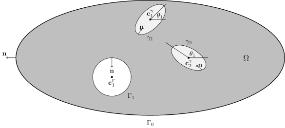
Figure 1: A sketch of a bounded fluid domain $\Omega$. $\gamma_{1}$ and $\gamma_{2}$ enclose rigid particles, while $\Gamma_{1}$ is a solid wall. If $\Omega$ is unbounded, $\Gamma_{0}$ is not present. The vector ${\mathbf{n}}$ is the unit normal vector pointing out of the fluid domain.

2.1 Governing Equations

We are interested in small particles and slow velocities which renders the Reynolds number small ${\mathrm{Re}}\ll 1$, and the fluid is governed by the incompressible Stokes equations. A Dirichlet boundary condition ${\mathbf{U}}$ is imposed on the solid walls $\Gamma$, a no-slip boundary condition is imposed on the rigid bodies $\gamma$, and the rigid bodies are assumed to be force- and torque-free. On each solid wall, there is a net force and torque, ${\mathbf{F}}^{\Gamma}_{i}$ and $L^{\Gamma}_{i}$, respectively, that depend on the boundary condition. A similar force, ${\mathbf{F}}^{\gamma}_{j}$, and torque $\L^{\gamma}_{j}$ are defined for each rigid body $\gamma_{j}$, but these, for the time being, are assumed to be 0. Therefore, the governing equations for $M_{p}$ particles suspended in a bounded $M_{w}$-connected domain is

$$\begin{split}\mu\Delta{\mathbf{u}}={\nabla}p,&\hskip 20.0pt{\mathbf{x}}\in\Omega,\hskip 14.45377pt&&\mbox{\em conservation of momentum,}\\ {\nabla}\cdot{\mathbf{u}}=0,&\hskip 20.0pt{\mathbf{x}}\in\Omega,\hskip 14.45377pt&&\mbox{\em conservation of mass,}\\ {\mathbf{u}}={\mathbf{U}},&\hskip 20.0pt{\mathbf{x}}\in\Gamma,\hskip 14.45377pt&&\mbox{\em wall velocity,}\\ {\mathbf{u}}={\mathbf{u}}^{\tau}_{j}+\omega_{j}({\mathbf{x}}-{\mathbf{c}}^{\gamma}_{j})^{\perp},&\hskip 20.0pt{\mathbf{x}}\in\gamma,\hskip 14.45377pt&&\mbox{\em no-slip on the bodies,}\\ {\mathbf{F}}_{j}^{\gamma}=0,&\hskip 20.0ptj=1,\ldots,M_{p},\hskip 14.45377pt&&\mbox{\em force-free bodies,}\\ L_{j}^{\gamma}=0,&\hskip 20.0ptj=1,\ldots,M_{p},\hskip 14.45377pt&&\mbox{\em torque-free bodies.}\end{split}$$ (2)

Here, ${\mathbf{u}}$ is the velocity, $p$ is the pressure, $\mu$ is the fluid viscosity, ${\mathbf{u}}^{\tau}_{j}$ and $\omega_{j}$ are the translational and rotational velocities of rigid body $j$, respectively, and ${\mathbf{F}}_{j}^{\gamma}$ and $L_{j}^{\gamma}$ are the net force and torque of rigid body $j$. In the Stokes limit, the fluid viscosity sets the time scale, and we assume it is one throughout the paper. In the case that the fluid domain is unbounded, the wall velocity equation is replaced with the far-field condition

$${\mathbf{u}}({\mathbf{x}})={\mathbf{u}}_{\infty}({\mathbf{x}}),\quad|{\mathbf{x}}|\rightarrow\infty.$$

Upon solving for the translational and rotational velocities, the rigid body centers and inclination angles $({\mathbf{c}}_{j},\theta_{j})$, $j=1,\ldots,M_{p}$, satisfy

$$\begin{split}\frac{d{\mathbf{c}}_{j}}{dt}={\mathbf{u}}^{\tau}_{j},\qquad\frac{d\theta}{dt}=\omega_{j}.\end{split}$$ (3)

Equations (2) and (3) govern the dynamics of the rigid body suspensions, and their numerical solution is a focus on this paper.

We have assumed that the rigid bodies are force- and torque-free. However, when two rigid bodies are brought sufficiently close together, numerical errors can cause the rigid bodies to unphysically intersect. To avoid contact, we will later relax the force- and torque-free conditions to guarantee that numerical errors do not cause rigid bodies to come into contact. This idea is first described for vesicle suspensions by Lu et al. [48] and we summarize the method in Section 2.3.

2.2 Boundary Integral Equation Representation

There exist many numerical methods for solving (2) such as level set methods [21], immersed boundary methods [54], dissipative particle dynamics [57], smoothed particle hydrodynamics [58], and lattice Boltzmann methods [41, 40]. However, because the fluid equations are linear a boundary integral equation (BIE) formulation [61] is possible. BIEs have several advantages including that only the interface has to be tracked, which simplifies the representation of complex and moving geometries, and high-order discretizations are straightforward. We now reformulate equation (2) as a BIE.

We start by formulating the incompressible Stokes equations in the absence of rigid bodies. The double-layer potential is the convolution of the stresslet with an arbitrary density function [42, 61],

$${\mathbf{u}}({\mathbf{x}})={\mathcal{D}}[{\bm{\eta}}]({\mathbf{x}})=\frac{1}{\pi}\int_{\Gamma}\frac{{\mathbf{r}}\cdot{\mathbf{n}}}{\rho^{2}}\frac{{\mathbf{r}}\otimes{\mathbf{r}}}{\rho^{2}}{\bm{\eta}}({\mathbf{y}})~{}\text{d}s_{{\mathbf{y}}},\quad{\mathbf{x}}\in\Omega,$$ (4)

where ${\mathbf{r}}={\mathbf{x}}-{\mathbf{y}}$, $\rho=|{\mathbf{r}}|$, and ${\bm{\eta}}$ is an unknown density function defined on ${\partial}\Omega$. The double-layer potential (4) satisfies the incompressible Stokes equations, and the Dirichlet boundary condition ${\mathbf{U}}$ is also satisfied if ${\bm{\eta}}$ satisfies [61]

$$-\frac{1}{2}{\bm{\eta}}({\mathbf{x}}_{0})+{\mathcal{D}}[{\bm{\eta}}]({\mathbf{x}}_{0})={\mathbf{U}}({\mathbf{x}}_{0}),\quad{\mathbf{x}}_{0}\in\Gamma.$$ (5)

The double-layer potential cannot represent rigid body motions that satisfy the incompressible Stokes equations. Following Power and Miranda [60, 59], this is resolved by introducing point forces and torques due to each interior component of the geometry $\Gamma_{j}$, and the strengths of these forces and torques are related to the density function ${\bm{\eta}}$. By introducing the velocity fields due to a point force (Stokeslet) and a point torque (rotlet), both centered at ${\mathbf{c}}$,

$$\mathbf{S}({\mathbf{x}},{\mathbf{c}})=\frac{1}{4\pi}\left(-\log\rho\mathbf{I}+\frac{{\mathbf{r}}\otimes{\mathbf{r}}}{\rho^{2}}\right),\quad\text{and}\quad\mathbf{R}({\mathbf{x}},{\mathbf{c}})=\frac{{\mathbf{r}}^{\perp}}{4\pi\rho^{2}},$$

where ${\mathbf{r}}={\mathbf{x}}-{\mathbf{c}}$ and $\rho=|{\mathbf{r}}|$. Then, the second-kind integral equation (5) is replaced with the completed second-kind BIE

$$\begin{split}-\frac{1}{2}{\bm{\eta}}({\mathbf{x}}_{0})+{\mathcal{D}}[{\bm{\eta}}]({\mathbf{x}}_{0})+\sum_{j=1}^{M_{w}}\left(\mathbf{S}({\mathbf{x}},{\mathbf{c}}^{\Gamma}_{j}){\mathbf{F}}^{\Gamma}_{j}+\mathbf{R}({\mathbf{x}},{\mathbf{c}}^{\Gamma}_{j})L^{\Gamma}_{j}\right)&={\mathbf{U}}({\mathbf{x}}_{0}),\quad&&{\mathbf{x}}_{0}\in\Gamma,\\ \int_{\Gamma_{j}}{\bm{\eta}}~{}\text{d}s&={\mathbf{F}}^{\Gamma}_{j},&&j=1,\ldots,M_{w},\\ \int_{\Gamma_{j}}{\bm{\eta}}\cdot({\mathbf{x}}-{\mathbf{c}}^{\Gamma}_{j})^{\perp}~{}\text{d}s&=L^{\Gamma}_{j},&&j=1,\ldots,M_{w}.\end{split}$$ (6)

We now introduce a suspension of rigid bodies $\gamma_{j}$, $j=1,\ldots,M_{p}$. The double-layer potential now includes contributions from both the solid walls and rigid bodies. Imposing the no-slip boundary condition on the rigid bodies, a BIE formulation of the suspension of rigid bodies governed by equation (2) is

$${\mathbf{U}}({\mathbf{x}}) =-\frac{1}{2}{\bm{\eta}}({\mathbf{x}})+{\mathcal{D}}[{\bm{\eta}}]({\mathbf{x}})+\sum_{j=1}^{M_{w}}\left(\mathbf{S}({\mathbf{x}},{\mathbf{c}}^{\Gamma}_{j}){\mathbf{F}}^{\Gamma}_{j}+\mathbf{R}({\mathbf{x}},{\mathbf{c}}^{\Gamma}_{j})L^{\Gamma}_{j}\right)$$

$$\hskip 96.0pt+\sum_{j=1}^{M_{p}}\left(\mathbf{S}({\mathbf{x}},{\mathbf{c}}^{\gamma}_{j}){\mathbf{F}}^{\gamma}_{j}+\mathbf{R}({\mathbf{x}},{\mathbf{c}}^{\gamma}_{j})L^{\gamma}_{j}\right),\quad{\mathbf{x}}\in\Gamma,$$ (7a)

$${\mathbf{u}}^{\tau}_{j}+\omega_{j}({\mathbf{x}}-{\mathbf{c}}_{j}^{\gamma})^{\perp} =-\frac{1}{2}{\bm{\eta}}({\mathbf{x}})+{\mathcal{D}}[{\bm{\eta}}]({\mathbf{x}})+\sum_{j=1}^{M_{w}}\left(\mathbf{S}({\mathbf{x}},{\mathbf{c}}^{\Gamma}_{j}){\mathbf{F}}^{\Gamma}_{j}+\mathbf{R}({\mathbf{x}},{\mathbf{c}}^{\Gamma}_{j})L^{\Gamma}_{j}\right)$$

$$\hskip 96.0pt+\sum_{j=1}^{M_{p}}\left(\mathbf{S}({\mathbf{x}},{\mathbf{c}}^{\gamma}_{j}){\mathbf{F}}^{\gamma}_{j}+\mathbf{R}({\mathbf{x}},{\mathbf{c}}^{\gamma}_{j})L^{\gamma}_{j}\right),\quad{\mathbf{x}}\in\gamma,$$ (7b)

$$\int_{\Gamma_{j}}{\bm{\eta}}~{}\text{d}s ={\mathbf{F}}^{\Gamma}_{j},\quad\int_{\Gamma_{j}}{\bm{\eta}}\cdot({\mathbf{x}}-{\mathbf{c}}^{\Gamma}_{j})^{\perp}~{}\text{d}s=L^{\Gamma}_{j},\quad j=1,\ldots,M_{w},$$ (7c)

$$\int_{\gamma_{j}}{\bm{\eta}}~{}\text{d}s ={\mathbf{F}}^{\gamma}_{j},\quad\int_{\gamma_{j}}{\bm{\eta}}\cdot({\mathbf{x}}-{\mathbf{c}}^{\gamma}_{j})^{\perp}~{}\text{d}s=L^{\gamma}_{j},\quad j=1,\ldots,M_{p},$$ (7d)

$${\mathbf{F}}^{\gamma}_{j} =0,\quad\L^{\gamma}_{j}=0,\quad j=1,\ldots,M_{p}.$$ (7e)

Again, the methodology of Power and Miranda relates the strength of the Stokeslets and rotlets of each rigid body to its density function. The BIE formulation (7) of the governing equations (2) consists of eight equations for eight unknowns: the density function, net force, and net torque on the solid walls and rigid bodies, and the translational and rotational velocities.

While (7a) and (7b) are both numerically desirable second-kind Fredholm integral equations equations, equation (7a) has a rank one null space because of the flux-free condition of the boundary data ${\mathbf{U}}$ [42]. Following [59], this null space is removed by adding the term

$$\mathcal{N}_{0}[{\bm{\eta}}]({\mathbf{x}})=\int_{\Gamma_{0}}{\mathbf{n}}({\mathbf{x}})\otimes{\mathbf{n}}({\mathbf{y}})~{}\text{d}s({\mathbf{y}})$$ (8)

to (7a), but only for points ${\mathbf{x}}\in\Gamma_{0}$. Finally, if $\Omega$ is unbounded, equation (7) has no null space, and the only modification is that equation (7a) is removed and equation (7b) has the background velocity ${\mathbf{u}}_{\infty}({\mathbf{x}})$ is added to its right hand side.

2.3 A Contact-Based Repulsion Force

Exact solutions of the Stokes equations prohibit contact between force- and torque-free bodies in finite time. Therefore, any contact between rigid bodies is caused by numerical errors. The two main sources of error are the quadrature error and time stepping error. We address the quadrature error using a combination of upsampling and interpolation, and details of the method are described in [62]. Time stepping methods have recently received a lot of attention, and some recent works address stiffness [62] and adaptive time stepping [39, 63, 74]. We describe time stepping methods in Section 3.3.

We adopt the method of using artificial forces to avoid contact, and there are many choices for the force. One possibility is a Morse or Lennard-Jones potential that grows as a high order polynomial as two bodies approach [24, 47]. This has been shown to work for dense suspensions, but the resulting ODEs for the rigid body dynamics become very stiff as the separation between bodies decreases. Spring models [80, 83, 34] have also been used to generate artificial repulsion forces, but these models also introduce stiffness. A further disadvantage of many contact algorithms is that they do not guarantee that particles remain contact-free.

We apply a modification of the contact-aware method of Lu et al. [48] that explicitly requires that particles remain contact-free. We only summarize the method, but a in-depth description is in [48]. The method starts with the Stokes equations in variational form,

$$\min\int_{\Omega}\nabla{\mathbf{u}}:\nabla{\mathbf{u}}~{}\text{d}\Omega,\quad\text{ such that }\quad\nabla\cdot{\mathbf{u}}=0,\quad{\mathbf{x}}\in\Omega.$$ (9)

After taking a time step, all pairs of bodies whose separation falls below a minimum separation distance, which includes those that have collided, are flagged. Then, the space-time interference volume (STIV), defined as the volume in space-time distance swept out by the trajectory of two bodies, is computed. Next, equation (9) is supplemented with an additional constraint that the STIV is positive (no contact). As detailed in [48, 29], STIV offer a metric to quantify collision volumes. By using computing the STIV, rather than simply the overlap at the new time step, time steps that result in rigid bodies passing through each other are detected and resolved. Details for solving (9) with the STIV inequality constraint are given in Section 3.2.

2.4 Computing the Pressure and Stress

To understand the rheological and statistical properties of suspensions of rigid bodies, it is necessary to compute the pressure, stress, and energy dissipation. This expressions are standard [59], but we summarize them for completeness. A numerical method for Computing the pressure, stress, and energy dissipation is described in Section 3.1.

The pressure of the two-dimensional double-layer potential is citePower1993

$$p({\mathbf{x}})=\frac{1}{\pi}\int_{\partial\Omega}\frac{1}{\rho^{2}}\left(\mathbf{I}-2\frac{{\mathbf{r}}\otimes{\mathbf{r}}}{\rho^{2}}\right){\mathbf{n}}\cdot{\bm{\eta}}~{}\text{d}s,\qquad{\mathbf{x}}\in\Omega.$$

The pressure of the Stokeslet and rotlet contributions are easily computed, and the pressure of the completed double-layer potential (6) is

$$p({\mathbf{x}})=\frac{1}{\pi}\int_{\partial\Omega}\frac{1}{\rho^{2}}\left(\mathbf{I}-2\frac{{\mathbf{r}}\otimes{\mathbf{r}}}{\rho^{2}}\right){\mathbf{n}}\cdot{\bm{\eta}}~{}\text{d}s+\sum_{i=1}^{M_{w}}\frac{{\mathbf{F}}_{i}^{\Gamma}\cdot({\mathbf{x}}-{\mathbf{c}}_{i}^{\Gamma})}{2\pi|{\mathbf{x}}-{\mathbf{c}}_{i}^{\Gamma}|^{2}}+\sum_{i=1}^{M_{p}}\frac{{\mathbf{F}}_{i}^{\gamma}\cdot({\mathbf{x}}-{\mathbf{c}}_{i}^{\gamma})}{2\pi|{\mathbf{x}}-{\mathbf{c}}_{i}^{\gamma}|^{2}}.$$ (10)

Starting with the pressure (10), we compute the stress tensor

$${\bm{\sigma}}=-p\mathbf{I}+\left(\nabla{\mathbf{u}}+(\nabla{\mathbf{u}})^{\intercal}\right),\qquad{\mathbf{x}}\in\Omega.$$

We decompose the stress into contributions from the double-layer potential, Stokeslets, and rotlets

$${\bm{\sigma}}={\bm{\sigma}}_{{\bm{\eta}}}+{\bm{\sigma}}_{S}+{\bm{\sigma}}_{R},$$ (11)

where

$${\bm{\sigma}}_{{\bm{\eta}}}({\mathbf{x}}) =\frac{1}{\pi}\int_{\partial\Omega}\left(\frac{{\mathbf{n}}\cdot{\bm{\eta}}}{\rho^{2}}\mathbf{I}-8\frac{({\mathbf{r}}\cdot{\mathbf{n}})({\mathbf{r}}\cdot{\bm{\eta}})({\mathbf{r}}\otimes{\mathbf{r}})}{\rho^{6}}+\frac{({\mathbf{r}}\cdot{\mathbf{n}})({\mathbf{r}}\otimes{\bm{\eta}}+{\bm{\eta}}\otimes{\mathbf{r}})}{\rho^{4}}+\frac{({\mathbf{r}}\cdot{\bm{\eta}})({\mathbf{r}}\otimes{\mathbf{n}}+{\mathbf{n}}\otimes{\mathbf{r}})}{\rho^{4}}\right)\text{d}s,$$

$${\bm{\sigma}}_{S}({\mathbf{x}}) =-\sum_{i=1}^{M_{w}}\frac{{\mathbf{F}}_{i}^{\Gamma}\cdot({\mathbf{x}}-{\mathbf{c}}_{i}^{\Gamma})}{\pi|{\mathbf{x}}-{\mathbf{c}}_{i}^{\Gamma}|^{2}}({\mathbf{x}}-{\mathbf{c}}_{i}^{\Gamma})\otimes({\mathbf{x}}-{\mathbf{c}}_{i}^{\Gamma})-\sum_{i=1}^{M_{p}}\frac{{\mathbf{F}}_{i}^{\gamma}\cdot({\mathbf{x}}-{\mathbf{c}}_{i}^{\gamma})}{\pi|{\mathbf{x}}-{\mathbf{c}}_{i}^{\gamma}|^{2}}({\mathbf{x}}-{\mathbf{c}}_{i}^{\gamma})\otimes({\mathbf{x}}-{\mathbf{c}}_{i}^{\gamma}),$$

$${\bm{\sigma}}_{R}({\mathbf{x}}) =-\sum_{i=1}^{M_{w}}\frac{L_{i}^{\Gamma}}{2\pi|{\mathbf{x}}-{\mathbf{c}}_{i}^{\Gamma}|^{2}}(({\mathbf{x}}-{\mathbf{c}}_{i}^{\Gamma})\otimes({\mathbf{x}}-{\mathbf{c}}_{i}^{\Gamma})^{\perp}+({\mathbf{x}}-{\mathbf{c}}_{i}^{\gamma})^{\perp}\otimes({\mathbf{x}}-{\mathbf{c}}_{i}^{\gamma}))$$

$$-\sum_{i=1}^{M_{p}}\frac{L_{i}^{\gamma}}{2\pi|{\mathbf{x}}-{\mathbf{c}}_{i}^{\gamma}|^{2}}(({\mathbf{x}}-{\mathbf{c}}_{i}^{\gamma})\otimes({\mathbf{x}}-{\mathbf{c}}_{i}^{\gamma})^{\perp}+({\mathbf{x}}-{\mathbf{c}}_{i}^{\gamma})^{\perp}\otimes({\mathbf{x}}-{\mathbf{c}}_{i}^{\gamma})).$$

These expressions hold inside $\Omega$. On the boundary there is a jump in the pressure and stress, as reported in [62]. These boundary terms are required for our near-singular integration scheme described in Section 3.1. Finally, using the divergence theorem, we the volumed average stresses can be expressed in terms of boundary integrals [61].

3 Numerical Methods

We are ultimately interested in studying statistical and rheological properties of the fiber suspensions. Therefore, we develop stable numerical methods that solve the governing equations (2) for long time horizons. To achieve high-order accuracy, the spatial grid is resolved with spectral accuracy (Section 3.1), and stability is achieved by using implicit interactions in the time integrator and adaptive time stepping (Section 3.3). We are much more concerned with stability than accuracy, so we use low-order but stable time stepping schemes. Each time step requires solving a block diagonal preconditioned dense linear system that is solved with GMRES and accelerated with the fast multipole method [25] (Section 3.4). We also discuss a numerical methods for the collision algorithm (Section 3.2), and for computing the pressure and stress (Section 3.5).

3.1 Spatial Discretization

Let ${\mathbf{x}}(\alpha)$, $\alpha\in[0,2\pi)$, be a parameterization of a rigid body $\gamma_{i}$. We will use a collocation method that requires the discretization points ${\mathbf{x}}_{k}$ at $k=1,\ldots,N_{p}$. Spectral accuracy is achieved by representing functions defined on $\gamma_{i}$ as a Fourier series

$$f(\alpha)=f({\mathbf{x}}_{i}(\alpha))=\sum_{k=0}^{N_{p}-1}\hat{f}_{k}e^{ik\alpha}.$$ (12)

The rigid walls are identically discretized at $N_{w}$ points and functions defined on the rigid walls are also represented with a Fourier series. We use the FFT to compute the Fourier coefficients, and all derivatives are computed with spectral accuracy using by differentiating in Fourier space.

With collocation points defined on the rigid walls and solid bodies, we now discretize the layer potentials. We use a Nyström method by approximating the double-layer potentials with the trapezoid rule. Equations (7) are discretized as

$${\mathbf{U}}({\mathbf{x}}_{i})=-\frac{1}{2}{\bm{\eta}}({\mathbf{x}}_{i})+\sum_{k=1}^{N}K({\mathbf{x}}_{i},{\mathbf{x}}_{k}){\bm{\eta}}({\mathbf{x}}_{k})\Delta s_{k} +\sum_{j=1}^{M_{p}}\left(\mathbf{S}({\mathbf{x}}_{i},{\mathbf{c}}^{\gamma}_{j}){\mathbf{F}}_{j}+\mathbf{R}({\mathbf{x}}_{i},{\mathbf{d}}_{j})L_{j}\right)$$

$$+\sum_{j=1}^{M_{w}}\left(\mathbf{S}({\mathbf{x}}_{i},{\mathbf{c}}^{\Gamma}_{j}){\mathbf{F}}_{j}+\mathbf{R}({\mathbf{x}}_{i},{\mathbf{c}}^{\Gamma}_{j})\L_{j}\right),\quad{\mathbf{x}}_{i}\in\Gamma,$$

for ${\mathbf{x}}_{i}\in\Gamma$, and

$${\mathbf{u}}^{\tau}_{j}+\omega_{j}({\mathbf{x}}_{i}-{\mathbf{c}}^{\gamma}_{j})^{\perp}=-\frac{1}{2}{\bm{\eta}}({\mathbf{x}}_{i})+\sum_{k=1}^{N}K({\mathbf{x}}_{i},{\mathbf{x}}_{k}){\bm{\eta}}({\mathbf{x}}_{k})\Delta s_{k} +\sum_{j=1}^{M_{p}}\left(\mathbf{S}({\mathbf{x}}_{i},{\mathbf{c}}^{\gamma}_{j}){\mathbf{F}}_{j}+\mathbf{R}({\mathbf{x}}_{i},{\mathbf{d}}_{j})L_{j}\right)$$

$$+\sum_{j=1}^{M_{w}}\left(\mathbf{S}({\mathbf{x}}_{i},{\mathbf{c}}^{\Gamma}_{j}){\mathbf{F}}_{j}+\mathbf{R}({\mathbf{x}}_{i},{\mathbf{c}}^{\Gamma}_{j})\L_{j}\right),$$

for ${\mathbf{x}}\in\gamma_{j}$, where $N=M_{w}N_{w}+M_{p}N_{p}$ is the total number of discretization points and

$$K({\mathbf{x}},{\mathbf{y}})=\frac{1}{\pi}\frac{{\mathbf{r}}\cdot{\mathbf{n}}}{\rho^{2}}\frac{{\mathbf{r}}\otimes{\mathbf{r}}}{\rho^{2}}$$

is the kernel of the double-layer potential. The diagonal entries of $K$ are replaced with the limiting value

$$\lim_{\begin{subarray}{c}{\mathbf{y}}\rightarrow{\mathbf{x}}\\ {\mathbf{y}}\in{\partial}\Omega\end{subarray}}K({\mathbf{x}},{\mathbf{y}})=\frac{\kappa}{2\pi}{\mathbf{t}}\otimes{\mathbf{t}},\quad{\mathbf{x}}\in{\partial}\Omega,$$

where $\kappa({\mathbf{x}})$ is the curvature and ${\mathbf{t}}({\mathbf{x}})$ is the tangent vector of ${\partial}\Omega$ at ${\mathbf{x}}$.

Since the kernel $K({\mathbf{x}},{\mathbf{y}})$ is smooth, the trapezoid rule guarantees spectral accuracy [79]. However, at a fixed resolution $N$, the error grows when a target point and a source point on different bodies are sufficiently close. The error is caused by a nearly-singular integrand with large derivatives. To resolve this issue, an algorithm for near-singular integration method must be employed. We use the interpolation scheme outlined in [62] that is based off of the algorithm first outlined in [82].

After discretizing (7) with a Nyström method, the result is a dense linear system for the density function, rotlets and Stokeslets, and the translational and rotational velocities of each body. We chose a double-layer potential formulation so that the linear system can be solved with a mesh-independent number of GMRES iterations [15]. Therefore, the algorithmic cost is dominated by the cost of a matrix-vector multiplication, and the number of required geometry-dependent GMRES iterations. Algorithms for controlling these costs are discussed in Section 3.4.

3.2 Contact Resolution

The contact resolution method starts by advancing the force- and torque-free bodies from time $t$ to $t+\Delta t$ with equation (3). Then, equation (9) needs to be solved with the inequality constraint that the STIV is greater than zero. The definition of the STIV includes a parameter that guarantees that not only do bodies intersect, but they maintain minimum separation distance. Following [48], we use a Lagrange multiplier, $\lambda$, to satisfy the non-negative STIV inequality constraint (a negative STIV indicates contact). The resulting equations are the incompressible Stokes equations with body forces and torques that depend on the gradient of the STIV, and the inequality constraint that the STIV is less than or equal to zero. Therefore, the governing equations are similar to (7), except that the force- and torque-free conditions have been changed.

The resulting equation is a non-linear complementary problem (NCP) To solve the NCP, the problem is linearized as a sequence of linear complementary problems (LCPs) that are solved until the STIV is less than or equal to zero. For small minimum separation distances, it is possible that the LCP converges very slowly, or not at all, to the solution of the NCP. In Section 3.3, we describe two methods to avoid this slow convergence.

If only two bodies are in contact, the symmetry of the STIV ensures that the net force is zero. However, if more than two bodies are in contact, then the forces returned by the STIV are not guaranteed to sum to zero. We improve the validity of the method by always requiring that the total force added to the system is zero, meaning

$$\sum_{j=1}^{M_{p}}{\mathbf{F}}^{\gamma}_{j}=\mathbf{0}.$$

To accomplish this, we group all bodies that are in contact into distinct clusters. For each cluster, the body that is in contact with the most other bodies (to break ties, the body with the largest repulsion force in magnitude) is given a net force that balances all other bodies in the cluster. Whenever a force on a body is scaled the torque on that body is scaled by the same amount.

3.3 Time Stepping Methods

Since we only consider rigid body suspensions, we only track the centers ${\mathbf{c}}_{i}^{\gamma}$ and orientations $\theta_{i}$ of each rigid body $\gamma_{i}$. Given a suspension of rigid bodies, (7) is solved for the translational and rotational velocities of each body. Then, the position and angle of each body are updated according to the ODEs,

$$\frac{\text{d}}{\text{d}t}{\mathbf{c}}_{k} ={\mathbf{u}}^{\tau}_{k},\quad{\mathbf{c}}_{k}(0)={\mathbf{c}}_{k}^{0},$$

$$\frac{\text{d}}{\text{d}t}\theta_{k} =\omega_{k},\quad\theta_{k}(0)=\theta_{k}^{0}.$$

The ODEs are advanced in time using the first-order explicit Euler method

$${\mathbf{c}}_{k}^{N+1} ={\mathbf{c}}_{k}^{N}+\Delta t\left({\mathbf{u}}_{k}^{\tau}\right)^{N},$$

$$\theta_{k}^{N+1} =\theta_{k}^{N}+\Delta t\left(\omega_{k}\right)^{N}.$$

A low cost first-order time stepper is justified since we are interested in statistical, rheological, and bulk quantities rather than the individual trajectories of the rigid bodies. If high-order accuracy is desired, a Runge-Kutta or deferred correction method [63, 65] can be applied.

Since the dynamics of the suspension can develop complex features, we use an heuristic adaptive time stepping method. When the LCP solver requires many iterations to solve the NCP, this indicates that the time step size should be reduced. Conversely, if the LCP solver converges quickly to the solution of the NCP, then a larger time step size can be taken. Therefore, if the each LCP iteration is not converging to a contact-free configuration sufficiently fast, we abort the time step and restart with the time step size $\Delta t/2$. Conversely, if the LCP iteration converges quickly, then, at the next time step, we increase $\Delta t$ to $1.5\Delta t$.

The stability of the method depends on the discretization of (7) and the minimum separation distance. If the minimum separation distance is small and the interaction between two nearly-touching bodies is discretized explicitly, then convergence of the LCP solver to the solution of the NCP requires a large number of iterations, and the maximum stable time step size is small. In contrast, if the interaction between the bodies is discretized implicitly, then the stiffness caused by the nearly-touching bodies is resolved and a larger stable time step can be taken.

The leading source of stiffness for a particular rigid body is the velocity field induced by the body itself. This can be controlled with a locally implicit discretization

$${\mathcal{D}}[{\bm{\eta}}]({\mathbf{x}})\approx{\mathcal{D}}^{n}[{\bm{\eta}}^{N+1}]({\mathbf{x}})+{\mathcal{D}}^{n}[{\bm{\eta}}^{N}]({\mathbf{x}}),$$ (13)

where the superscript of ${\mathcal{D}}$ implies that the geometry used in the discretization of the layer potential is at time step $n$. This time stepping method is focus of the work of Lu et al. [48]. There, to avoid stiffness caused by nearly-touching bodies, a sufficiently large minimum separation distance is used.

Instead of avoiding nearly-touching bodies, we use the globally implicit discretization

$${\mathcal{D}}[{\bm{\eta}}]({\mathbf{x}})\approx{\mathcal{D}}^{N}[{\bm{\eta}}_{N+1}]({\mathbf{x}})+{\mathcal{D}}^{N}[{\bm{\eta}}^{N+1}]({\mathbf{x}}).$$ (14)

By discretizing the interactions between different bodies implicitly, the stiffness caused by nearly-touching bodies is reduced, so large time steps with small minimum separation distances are possible.

3.4 Fast Summation and Preconditioning

A discretization of the locally implicit time stepper (13) results in a block-diagonal linear system, where each block is a dense $N_{p}\times N_{p}$ or $N_{w}\times N_{w}$ matrix. In contrast, a discretization of the globally implicit time stepper (14) results in a dense $N\times N$ linear system. Therefore, considering only the rigid body contributions, the cost of a single matrix-vector multiplication is $\mathcal{O}(M_{p}N_{p}^{2})$ for (13) and $\mathcal{O}(M_{p}^{2}N_{p}^{2}$ for (14). We reduce the cost of matrix-vector multiplication by using the fast multipole method. This reduces the cost of a single matrix-vector multiplication for both the locally implicit and globally implicit time stepping methods to $\mathcal{O}(N)$ operations.

Reducing the cost of matrix-vector multiplication greatly reduces the computational effort. However, for dense suspensions, the number of GMRES iterations can also be large. Therefore, we apply a block-diagonal preconditioner where each block is precomputed and factorized. The identical preconditioner has been used for two-dimensional vesicle suspensions [62]. For rigid bodies, the preconditioner is further accelerated by factorizing all double-layer potentials at the initial condition, and then multiplying with rotation matrices corresponding to the rotation velocity $\omega$.

3.5 Computing the Pressure and Stress

Computing the pressure (10) and stress (11) are more challenging than evaluating the velocity double-layer potential. The challenge stems from a singularity that scales as $\mathcal{O}(|{\mathbf{x}}-{\mathbf{y}}|^{-2})$ as a target point approaches a source point. The pressure and stress are computed using a combination of singularity subtraction and odd-even integration [72]. The result is a spectrally accurate method for computing the pressure and stress.

Near-singular integration still required, and our interpolation-based method requires limiting values of the layer potentials (10) and (11) as ${\mathbf{x}}\rightarrow{\partial}\Omega$. The limiting values and tests of the near-singular integration scheme are reported in [62].

4 Results

We use our new time stepping method to simulate bounded and unbounded suspensions of two-dimensional rigid bodies in a viscous fluid. The main parameters are the minimum separation distance $\delta$, the number of discretization points of each body, $N_{p}$, and each solid wall, $N_{w}$, and the initial time step size $\Delta t$. We perform convergence studies and investigate the effect of the STIV algorithm on the reversibility of the flow. To further demonstrate the consequence of STIV, we include plots of streamlines that cross whenever the collision detection algorithm is applied. The particular experiments we perform are now summarized.

• Shear Flow: We consider the standard problem of two identical rigid circles in the shear flow ${\mathbf{u}}=(y,0)$ with the left body slightly elevated from the right body. We report similar results to those presented in [48], but we are able to take smaller initial displacements and minimum separation distances. The contact algorithm breaks the reversibility of the flow, and this effect is illustrated and quantified.

• Taylor-Green Flow: We simulate a concentrated suspension of 48 rigid ellipses in an unbounded Taylor-Green flow. At the prescribed separation distance, our new time stepping method is able to stably reach the time horizon, while the locally semi-implicit time integrator proposed by Lu et al. [48] results in the STIV algorithm stalling, even with $\Delta t=10^{-8}$.

• Porous Monolayer Injection: We consider a suspension of confined rigid circular bodies motivated by an experiment by MacMinn et al. [50]. The geometry is an annulus with an inflow at the inner boundary and an outflow at the outer boundary. We again examine the effect STIV on the reversibility of the flow, and compute the shear strain rate and make qualitative comparisons to results for deformable bodies [50].

• Taylor-Couette Flow: With the ability to do high area fraction suspensions without imposing a large non-physical minimum separation distance, we simulate rigid bodies of varying aspect ratios inside a Taylor-Couette device. We examine the effect of the rigid body shape and area fraction on the effective viscosity and the alignment angles.

4.1 Shear Flow

We consider two rigid circular bodies in the shear flow ${{\mathbf{u}}}({\mathbf{x}})=(y,0)$. One body is centered at the origin, while the other body is placed to the left and slightly elevated of the origin. With this initial condition, the particles come together, interact, and then separate. Both bodies are discretized with $N=32$ points and the arc length spacing $h=2\pi/32\approx 0.196$. This experiment was also performed by Lu et al. [48], and we compare the two time stepping methods.

We start by considering the time step size $\Delta t=0.4$ and minimum separation distance $\delta=0$ (no contact algorithm). Our new globally implicit method successfully reaches the time horizon without requiring a repulsion force. However, with the same $\Delta t$, the local explicit time stepping results in a collision between the bodies, so the collision algorithm is required to reach the time horizon. Alternatively, the time step size can be reduced, but, as we will see, for sufficiently dense suspensions, even an excessively small time step size results in collisions. Next, in Figure 2, we investigate the effect of the minimum separation distance on the position of the rigid bodies. The top plot shows the trajectory of the left body as it approaches, interacts, and finally separates from the body centered at the origin. In this simulation, we use our new globally implicit time integrator, but the STIV contact algorithm is not applied. The bottom left plot shows the trajectory of the particle when the contact algorithm is applied with varying levels of separation. Notice that the trajectories are identical until near $x=0$ when the particle separation first falls below the minimum separation distance. Finally, in the bottom right plot, the final vertical displacement body initially on the left is plotted. These results are computed for the locally implicit time stepping method [48], and the general trend of the trajectories are similar.

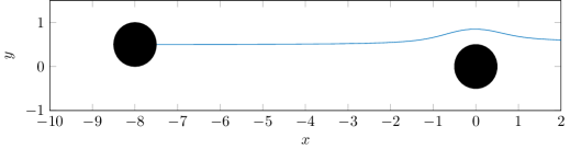
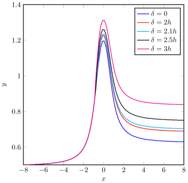
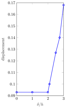
Figure 2: Shear experiment. Top: The initial setup and trajectory of the left body. Bottom left: The left body’s trajectory for varying minimum separation distances. Notice how the trajectories are identical until shortly before $x=0$ when the contact algorithm is first applied. Bottom right: The final vertical displacement of the left particle for varying minimum separation distances.

We next investigate the effect of the collision algorithm on the time reversibility of the flow. We reverse the shear direction at $t=10$ and measure the error between the body’s center at $t=0$ and $t=20$. We expect an error that is the sum of a first-order error caused by time stepping, and a fixed constant caused by the minimum separation distance. The results for various values of $\delta$ are reported in Table 1. When the contact algorithm is not applied when $\delta=0$ and $\delta=h$, we observe the expected first-order convergence. When $\delta\geq 2h$, the bodies are deflected onto contact-free streamlines when their proximity reaches the minimum separation distance. After the flow is reversed, the bodies again pass one another, but they are now on contact-free streamlines, so the initial deflection is not reversed. For these larger values of $\delta$, we see in Table 1 that the error eventually plateaus as $\Delta t$ is decreased.

			$\Delta t$
$\delta$	$4\times 10^{-2}$	$2\times 10^{-2}$	$1\times 10^{-2}$	$5\times 10^{-3}$	$2.5\times 10^{-3}$
0	$1.35\times 10^{-1}$	$7.32\times 10^{-2}$	$3.74\times 10^{-2}$	$2.00\times 10^{-2}$	$1.01\times 10^{-2}$
$h$	$1.35\times 10^{-1}$	$7.32\times 10^{-2}$	$3.74\times 10^{-2}$	$2.00\times 10^{-2}$	$1.01\times 10^{-2}$
$2h$	$1.88\times 10^{-1}$	$1.41\times 10^{-1}$	$1.17\times 10^{-1}$	$1.08\times 10^{-1}$	$1.02\times 10^{-1}$
$2.25h$	$2.55\times 10^{-1}$	$2.08\times 10^{-1}$	$1.87\times 10^{-1}$	$1.78\times 10^{-1}$	$1.73\times 10^{-1}$
$2.50h$	$3.05\times 10^{-1}$	$2.69\times 10^{-1}$	$2.52\times 10^{-1}$	$2.45\times 10^{-1}$	$2.40\times 10^{-1}$
$2.75h$	$3.64\times 10^{-1}$	$3.31\times 10^{-1}$	$3.13\times 10^{-1}$	$3.07\times 10^{-1}$	$3.03\times 10^{-1}$
$3.00h$	$4.12\times 10^{-1}$	$3.88\times 10^{-1}$	$3.72\times 10^{-1}$	$3.67\times 10^{-1}$	$3.63\times 10^{-1}$

Table 1: A study of time reversibility of the shear flow example. At $t=10$, the flow direction is reversed and we calculate the relative error in the initial and final positions. When the collision constraint is active and force is needed to keep the bodies apart the error in the reversibility is dominated by the contact algorithm.

The break in reversibility is further demonstrated by examining individual streamlines. In Figure 3, we compute the streamline of the left body for three different initial placements. We set $\delta=3h$ for all the streamlines. With this threshold, only the bottom-most streamline falls below $\delta$. Therefore, as the bodies approach, the streamlines behave as expected—they do not cross. However, when the contact algorithm is applied to the blue streamline, the streamlines cross.

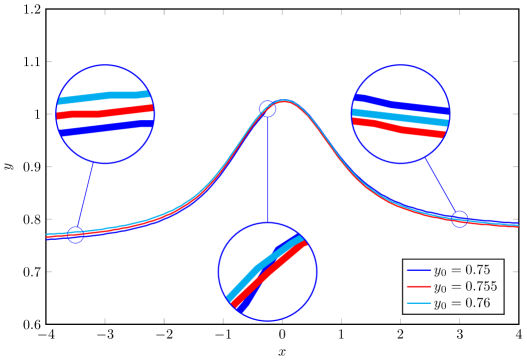
Figure 3: The contact algorithm causes streamlines to cross. Keeping the minimum separation fixed at $\delta=3h$, we vary the starting $y$ location of the left body. The teal and red streamlines do not require a repulsion force to enforce the minimum separation between the bodies, but the blue streamline does. Once the contact algorithm is applied, the blue streamline crosses the other streamlines (middle inset). This crossing of the streamlines breaks the reversibility of the simulation.

4.2 Taylor-Green Flow

For planar flows, we can separate suspensions into dilute and concentrated regimes by comparing the number of bodies per unit area, $\nu$, to the average body length $\ell$. If $\nu<1/\ell^{2}$, then we are in the dilute regime, otherwise we are in the concentrated regime (in 2D planar suspensions, unlike 3D suspensions, there is no semi-dilute regimes). We consider the suspension of 75 rigid bodies in the Taylor-Green flow $\mathbf{u}^{\infty}=(\cos(x)\sin(y),-\sin(x)\cos(y))$. The number of bodies per unit area is $\nu\approx 3.1$ which is greater than $1/\ell^{2}=1.1$. Therefore, this suspension is well within the concentrated regime.

We discretize the bodies with $N=32$ points and select the minimum separation distance $\delta=0.05h$. Snapshots of the simulation are shown in Figure 4. In this concentrated suspension, the bodies come into contact much more frequently. If the interactions between these nearly touching bodies are treated explicitly, this leads to stiffness. Our time stepper controls this stiffness by treating these interactions implicitly, and the simulation successfully reaches the time horizon. We performed the same simulation, but with the locally implicit time stepping method [48]. Because of the near-contact, smaller time step sizes must be taken. We took time step sizes as small as $10^{-8}$, and the method was not able to successfully reach the time horizon. This exact behavior has also been observed for vesicle suspensions [62]. In the bottom right plot of Figure 4, we show the trajectory of one body for different time step sizes. The dots denote locations where the contact algorithm is applied. For this very complex flow, the trajectories are in good agreement with different time step sizes.

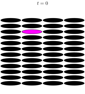
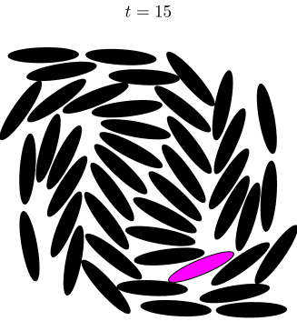
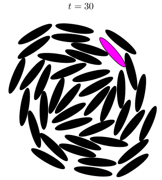
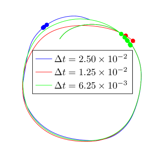
Figure 4: Snapshots of a dense suspension in an unbounded Taylor-Green flow. The number of bodies per unit area $\nu$ is approximately 3.1. This is greater than $1/\ell^{2}=1.1$, which puts the simulation well within the concentrated regime. Bodies are discretized with 32 points and the minimum separation is $\delta=0.05h$. The bottom right plot shows the trajectory of the center of the colored body for different step sizes. Each line in that plot is marked where a repulsion force is used to enforce the minimum separation.

4.3 Fluid Driven Deformation

A recent experiment considers a dense monolayer packing of soft deformable bodies [50]. Motivated by this experiment, we perform numerical simulations of rigid bodies in a similar device. We pack rigid bodies in a Couette device, but with a very small inner boundary. The boundary conditions are an inflow or outflow of rate $Q$ at the inner boundary with an outflow or inflow at the outer cylinder. This boundary condition corresponds to injection and suction of fluid from the center of the experimental microfluidic device. In the experimental setting, the soft bodies are able to reach the outer boundary, and the resulting boundary condition would not be uniform at the outer wall. So that we can apply the much simpler uniform inflow or outflow at the outer boundary, we force the rigid bodies to remain well-separated from the outer wall. We accomplish this by placing a ring of fixed rigid bodies halfway between the inner and outer cylinders (Figure 5). The spacing between these fixed bodies is sufficiently small that the mobile bodies are not able to pass. Since the outer boundary is well-separated from the fixed bodies, the outer boundary condition is justifiably approximated with a uniform flow.

Figure 5: The geometry used in our numerical experiment that is motivated by the experimental setup of MacMinn et al. [50]. The fixed solid bodies are shaded in black.

We start by examining the effect of the contact algorithm on the reversibility of the flow. We again reverse the flow at time $T$ and run the simulation until time $2T$. The rigid bodies are in contact for much longer than the shear example in Section 4.1, so maintaining reversibility is much more challenging. Figure 6 shows several snapshots of the simulation, and the bottom right plot superimposes the initial and final configurations. We observe only a minor violation of reversibility, and it is largest for bodies that were initially near the fixed bodies—the contact algorithm is applied to these bodies most frequently.

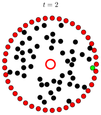
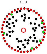
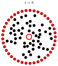
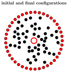
Figure 6: Snapshots of a rigid body suspension motivated by an experiment for deformable bodies [50]. Fluid is injected at a constant rate starting at $t=0$. At $t=4$ the flow direction is reversed. Fixed bodies are colored in red, while bodies subject to a repulsion force are colored in green. The initial configuration has been superimposed on the final configuration at $t=8$ to show the effect of the repulsion forces on reversibility.

In [50], the shear strain rate is measured to better characterize the flow. In Figure 7, we compute and plot the shear strain rate for the simulation in Figure 6. A qualitative comparison of the numerical and experimental results are in good agreement. In particular, the petal-like patterns in Figure 7 are also observed in the experimental results.

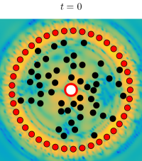
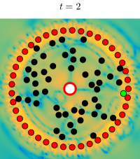
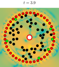
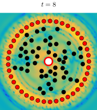
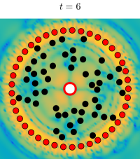
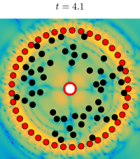
Figure 7: The shear strain rate $\log_{10}(|\sigma_{xy}|)$ of the suspension in Figure 6. The formation of the petal-like patterns is also observed for the suspension of deformable bodies [50].

4.4 Taylor-Couette Flow

In many industrial applications, for example pulp and paper manufacturing, suspensions of rigid elongated fibers are encountered. Motivated by these suspensions we investigate rheological and statistical properties of confined suspensions. We consider suspensions of varying area fraction and body aspect ratio; specifically we will look at 5, 10, and 15 percent area fractions and elliptical bodies of aspect ratio, $\lambda$ of 1, 3, and 6. In all the examples, $nuM1/ell^{2}$, so all the suspensions are in the dilute regime. The bodies initial locations are random, but non-overlapping (Figure 8). The flow is driven by rotating the outer cylinder at a constant angular velocity while the inner cylinder remains fixed.

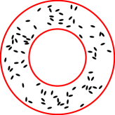
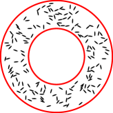
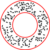
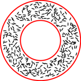
Figure 8: Four initial configurations for Taylor-Couette flow with varying volume fraction $\phi$ and aspect ratio $\lambda$. From left to right: 1) $\phi=5\%$, $\lambda=3$, 2) $\phi=5\%$, $\lambda=6$, 3) $\phi=10\%$, $\lambda=3$, 4) $\phi=10\%$, $\lambda=6$.

Before measuring any rheological properties, we complete one full revolution of the outer wall so that the bodies are well-mixed and approaching a statistical equilibrium. We start by considering the alignment of the bodies. The alignment is particularly insightful since many industrial processes involve fibers suspended in a flow, and the alignment affects the material properties [43]. One way to measure the alignment is the order parameter, $S$ defined as,

$$S=\left\langle\frac{d\cos^{2}\tilde{\theta}-1}{d-1}\right\rangle,$$

where $d$ is the dimension of the problem ($2$ in our case), $\tilde{\theta}$ is the deviation from the expected angle, and $\langle\cdot\rangle$ averages over all bodies. If $S=1$, all bodies are perfectly aligned with the shear direction, $S=0$ corresponds to a random suspension (no alignment), and $S=-1$ means that all bodies are perfectly aligned perpendicular to the shear direction. In our geometric setup, a body centered at $(x,y)$ has an expected angle of $\tilde{\theta}\tan^{-1}(y/x)+\pi/2$, and the average alignment of the bodies will be in the direction of the shear, which is also perpendicular to the radial direction.

Since the initial condition is random, the initial configurations in Figure 8 have an order parameter $S\approx 0$. As the outer cylinder rotates, we see in Figure 9 that $S$ increases quite quickly. The area fractions $\phi$ we consider have a minor effect on $S$; however, the aspect ratio has a large effect. In particular, suspensions with slender bodies align much better with the flow.

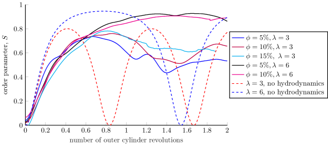
Figure 9: The order parameter of different fiber concentrations and aspect ratios. We see that the 6:1 fibers align better. The 6:1 fibers rotate rotate through the angle perpendicular to the shear direction more quickly than the 3:1 fibers and thus spend more time approximately aligned with the shear direction. The dashed lines represent the order parameter for a suspension in an unbounded shear flow with bodies that do not interact hydrodynamically. The red line shows $\lambda=3$, while the blue line shows $\lambda=6$.

This matches the known dynamics of a single body in an unbounded shear flow, where the body will align with the shear direction on average. Bodies with a high aspect ratio rotate quickly when then they are perpendicular to the shear direction and spend more time nearly aligned with the shear direction. We compare our results to the time averaged order parameter of a single elliptical body in an unbounded shear flow. If the shear rate is $\dot{\gamma}$, the body rotates with period $\tau=\pi/(2|\dot{\gamma}|)(\lambda+\lambda^{-1})$ [32] according to

$$\varphi(t)~{}=~{}\tan^{-1}\left(\frac{1}{\lambda}\tan\left(\frac{\lambda\dot{\gamma}t}{\lambda^{2}+1}\right)\right).$$

The time average order parameter is then,

$$\langle S\rangle~{}=~{}\frac{1}{\tau}\int_{0}^{\tau}\left(2\cos^{2}(\varphi(t))-1\right)~{}\text{d}t~{}=~{}\frac{\lambda-1}{\lambda+1}.$$

Independent of shear rate, for $\lambda=3$ the theoretical $\langle S\rangle$ is 1/2 and for $\lambda=6$ it is 5/7. Table 2 shows the time and space averaged order parameter for the Couette apparatus.We see that in all cases our computed time averaged order parameter is higher than the theoretical single fiber case. This could be due to the hydrodynamic interactions between the bodies, or the effect of the solid walls.

In the absence of solid walls and hydrodynamic interactions between bodies, a suspension will align and disalign. The period of the order parameter in this case is the same as the rotational period for a single fiber. In Figure 9 the theoretical order parameter is shown for a suspension of non-hydrodynamically interacting fibers in an unbounded shear flow. Hydrodynamic interactions prevent the suspension from disaligning completely.

area fraction, $\phi$	aspect ratio, $\lambda$	computed $\langle S\rangle$	theoretical $\langle S\rangle$ (single fiber)
5%	3	0.52	0.50
10%	3	0.60	0.50
15%	3	0.65	0.50
5%	6	0.91	0.71
10%	6	0.89	0.71

Table 2: The time averaged order parameter during the second revolution of the Couette apparatus. The higher aspect ratio fibers align better on average. The alignment is in all cases higher than predicted for a single Jeffery orbit.

Another quantity of interest in rheology is the effective viscosity of a suspension. The shear viscosity $\mu$ relates the bulk shear stress $\sigma_{xy}$ of a Newtonian fluid to the bulk shear rate $\dot{\gamma}$,

$$\sigma_{xy}=\mu\dot{\gamma}.$$

Adding bodies increases the bulk shear stress of a suspension. The proportionality constant relating the increased $\sigma_{xy}$ to the shear rate is the apparent viscosity, and the ratio between the apparent viscosity and the bulk viscosity is the effective viscosity $\mu_{\text{eff}}$. Experimentally, the bulk shear stress is often computed by measuring the torque on the inner cylinder [38]. Numerically, this is simply the strength of the rotlet centered in the inner cylinder. By computing the ratio of the torque on the inner cylinder with bodies to the torque without bodies we determine the effective viscosity of a suspension. Figure 10 shows the effective viscosity increases with $\phi$, but is generally lower for bodies with aspect ratio $\lambda=6$. This is because higher aspect ratio bodies align themselves better, and thus contribute less to the bulk shear stress. The spikes in 10 occur when a repulsion force is added to the system. Similar spikes were observed numerically in [48]. To make the results more clear we have used a multiscale local polynomial transform to smooth the data shown in Figure 10.

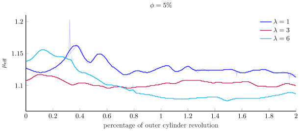
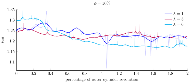
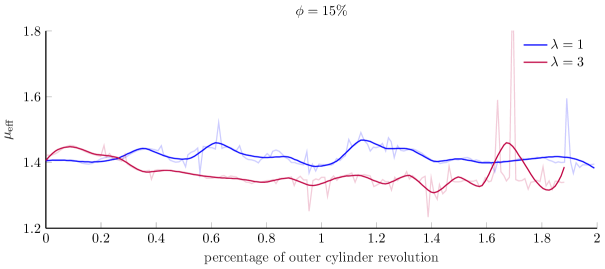
Figure 10: Instantaneous bulk effective viscosity for various volume fractions and body aspect ratios. The inner cylinder is fixed, while the outer one rotates at a constant angular velocity. The transparent lines represent the raw data, while the solid lines have been smoothed using a multiscale local polynomial transform.

Finally, instead of computing the instantaneous effective viscosity, experimenters are interested in the time averaged effective viscosity of a suspension. In Table 3, we report the average instantaneous effective viscosity over the second revolution of the outer cylinder

$\lambda$	5% area fraction	10% area fraction	15% area fraction
1	1.12	1.22	1.42
3	1.10	1.23	1.36
6	1.08	1.18

Table 3: Time averaged effective viscosity for various area fractions and aspect ratios. The time average is done between the first and second revolutions of the outer cylinder. As $\phi$ increases the effective viscosity increases as expected. In general higher aspect ratio bodies increase the viscosity less.

5 Conclusions

We have developed a stable time stepping method for simulating dense suspensions of rigid bodies without introducing stiffness or requiring a large minimum separation distance. A contact algorithm is used that is guaranteed to avoid overlap. Using this new time stepper we are able to simulate concentrated suspensions with a large time step and a small minimum separation distance. We verify that our new globally implicit time stepping method is able to take larger stable time step sizes when compared to a locally implicit time stepping method.

The contact algorithm is not reversible, and we examine the net effect on the reversibility of the flow. We compare the initial and final configurations of two suspensions where the flow is reversed halfway through the simulation. The simulations demonstrate that the error in the reversibility is the expected sum of the time stepping error and the error introduced by the contact algorithm.

We use the new time stepping method to compute rheological properties of suspensions including order parameters, effective viscosities, and strain rates. These rheological properties are compared with known order parameters for of Jeffery orbits and the strain rate observed in an experiment for deformable bodies.

There are several outstanding issues with this method. The most obvious is that the suspensions are two-dimensional. All the individual algorithms we have developed in three dimensions. However, to simulate similar results with respect to volume fraction, minimum separation distances, and aspect ratios, the spatial resolution will have to be reduced, and this will still require parallel algorithms and low-resolution algorithms [34].

A recent publication considers three-dimensional simulations of rigid bodies [17], but uses a different contact algorithm than the STIV we used. It is unclear that this contact algorithm will be able to resolve dense suspensions where there are many contacts. As an alternative to the STIV, the contact can be measured only at the final configuration, rather than as a space-time volume. However, this collision metric indicates a contact-free configuration when two particles pass through one another. Therefore, we prefer to use the STIV contact algorithm, which has been developed in three dimensions [29], but it has not yet been applied to suspensions.

Even with the development of our new time stepping method, we observe difficult cases. First, a good contact model between mobile bodies and fixed rigid walls needs to be developed. Second, the LCP solver can converge slowly or not at all to a contact-free suspension. While the adaptive time stepping method helps alleviate some of these instances, it is clear that additional algorithms are needed. Moreover, a more reliable algorithm for choosing an optimal time step size would help avoid instances where the time step size is reduced many times before a time step is finally accepted.

References

References

- [1] Suresh G. Advani and Charles L. Tucker III. The Use of Tensors to Describe and Predict Fiber Orientation in Short Fiber Composites. Journal of Rheology, 31(8):751–784, 1987.
- [2] Suresh G. Advani and Charles L. Tucker. Closure approximations for three-dimensional structure tensors. Journal of Rheology, 34(3):367–386, 1990.
- [3] Ludvig af Klinteberg and Anna-Karin Tornberg. Fast Ewald summation for Stokesian particle suspensions. International Journal for Numerical Methods in Fluids, 76(10):669–698, 2014.
- [4] Ludvig af Klinteberg and Anna-Karin Tornberg. A fast integral equation method for solid particles in viscous flow using quadrature by expansion. Journal of Computational Physics, 326:420–445, 2016.
- [5] G. Ausias, X.J. Fan, and R.I. Tanner. Direct simulation for concentrated fibre suspensions in transient and steady state shear flows. Journal of Non-Newtonian Fluid Mechanics, 135(1):46–57, 2006.
- [6] J. Barnes and P. Hut. A hierarchical force-calculation algorithm. Nature Publishing Group, 324:446–449, 1986.
- [7] Alex Barnett, Bowei Wu, and Shravan Veerapaneni. Spectrally-Accurate Quadratures for Evaluation of Layer Potentials Close to the Boundary for the 2D Stokes and Laplace Equations. SIAM Journal on Scientific Computing, 37(4):B519–B542, 2015.
- [8] G. K. Batchelor. Slender-body theory for particles of arbitrary cross-section in Stokes flow. Journal of Fluid Mechanics, 44:419, 1970.
- [9] G. K. Batchelor. The stress system in a suspension of force-free particles. Journal of Fluid Mechanics, 41(3):545–570, 1970.
- [10] G. K. Batchelor. The stress generated in a non-dilute suspension of elongated particles by pure straining motion. Journal of Fluid Mechanics, 46(4):813–829, 1971.
- [11] J. Thomas Beale, Wenjun Ying, and Jason R. Wilson. A Simple Method for Computing Singular or Nearly Singular Integrals on Closed Surfaces. Communications in Computational Physics, 20(3):733–753, 2016.
- [12] Miguel Angel Bibbó. Rheology of semiconcentrated fiber suspensions. PhD thesis, Massachusetts Institute of Technology, 1987.
- [13] A. Brandt and A. A. Lubrecht. Multilevel matrix multiplication and fast solution of integral equations. Journal of Computational Physics, 90(2):348–370, October 1990.
- [14] F. P. Bretherton. The motion of rigid particles in a shear flow at low Reynolds number. Journal of Fluid Mechanics, 14:284, 1962.
- [15] S. L. Campbell, I. C. F. Ipsen, C. T. Kelley, C. D. Meyer, and Z. Q. Xue. Convergence estimates for solution of integral equations with GMRES. Journal of Integral Equations and Applications, 8(1):19–34, 1996.
- [16] Ke Chen. An Analysis of Sparse Approximate Inverse Preconditioners for Boundary Integral Equations. SIAM Journal on Matrix Analysis and Applications, 22(4):1058–1078, 2000.
- [17] Eduardo Corona, Leslie Greengard, Manas Rachh, and Shravan Veerapaneni. An integral equation formulation for rigid bodies in Stokes flow in three dimensions. Journal of Computational Physics, 332:504–519, 2017.
- [18] Pieter Coulier, Hadi Pouransari, and Eric Darve. The Inverse Fast Multipole Method: Using a Fast Approximate Diret Solver as a Preconditioner for Dense Linear Systems. SIAM Journal on Scientific Computing, 39(3):A761–A796, 2017.
- [19] Steven M. Dinh and Robert C.!Armstrong. A Rheological Equation of State for Semiconcentrated Fiber Suspensions. Journal of Rheology, 28(3):207–227, 1984.
- [20] M. Doi and S. F. Edwards. Dynamics of rod-like macromolecules in concentrated solution. Part 1. Journal of the Chemical Society, Faraday Transactions 2: Molecular and Chemical Physics, 74:560–570, 1978.
- [21] Hua-Shu Dou, Boo Cheong Khoo, Nhan Phan-Thien, Khoon Seng Yeo, and Rong Zheng. Simulations of fibre orientation in dilute suspensions with front moving in the filling process of a rectangular channel using level-set method. Rheologica Acta, 46(4):427–447, 2007.
- [22] Xijun Fan, N. Phan-Thien, and Rong Zheng. A direct simulation of fibre suspensions. Journal of Non-Newtonian Fluid Mechanics, 74(1):113–135, 1998.
- [23] Julien Férec, Emmanuelle Abisset-Chavanne, Gilles Ausias, and Francisco Chinesta. On the use of interaction tensors to describe and predict rod interactions in rod suspensions. Rheologica Acta, 53(5):445–456, Jun 2014.
- [24] Daniel Flormann, Othmane Aouane, Lars Kaestner, Christian Ruloff, Chaouqi Misbah, Thomas Podgorski, and Christian Wagner. The buckling instability of aggregating red blood cells. Scientific Reports, 7:7928, 2017.
- [25] Anne Greenbaum, Leslie Greengard, and Anita Mayo. On the numerical solution of the biharmonic equation in the plane. Physica D: Nonlinear Phenomena, 60(1):216–225, 1992.
- [26] L. Greengard and V. Rokhlin. A Fast Algorithm for Particle Simulations. Journal of Computational Physics, 135(2):280–292, 1987.
- [27] Elisabeth Guazzelli and Jeffey F. Morris. A Physical Introduction of Suspension Dynamics. Cambridge University Press, Cambridge, UK, 2011.
- [28] K. Gustavsson and A.-K. Tornberg. Gravity induced sedimentation of slender fibers. Physics of Fluids, 21:123301, 2009.
- [29] David Harmon, Daniele Panozzo, Olga Sorkine, and Denis Zorin. Interference-aware Geometric Modeling. ACM Transactions on Graphics, 30(6):137:1–137:10, 2011.
- [30] Johan Helsing and Rikard Ojala. On the evaluation of layer potentials close to their sources. Journal of Computational Physics, 227:2899–2921, 2008.
- [31] PW Hemker and H Schippers. Multiple grid methods for the solution of Fredholm integral equations of the second kind. Mathematics of Computation, 36(153):215–232, 1981.
- [32] G. B. Jeffery. The Motion of Ellipsoidal Particles Immersed in a Viscous Fluid. Proceedings of the Royal Society of London Series A, 102:161–179, 1922.
- [33] C. G. Joung, N. Phan-Thien, and X.J. Fan. Direct simulation of flexible fibers. Journal of Non-Newtonian Fluid Mechanics, 99(1):1–36, 2001.
- [34] Gökberk Kabacaoğlu, Bryan Quaife, and George Biros. Low-resolution simulations of vesicle suspensions in 2D. Journal of Computational Physics, 357:43–77, 2018.
- [35] Seppo J. Karrila and Sangtae Kim. Integral Equations of the Second Kind for Stokes Flow: Direct Solutions for Physical Variables and Removal of Inherent Accuracy Limitations. Chemical Engineering Communications, 82(1):123–161, 1989.
- [36] Sangtae Kim and Seppo J. Karrila. Microhydrodynamics: Principles and Selected Applications. Butterworth-Heinemann, Stoneham, MA, 1991.
- [37] Andreas Klöckner, Alexander Barnett, Leslie Greengard, and Michael O’Neil. Quadrature by expansion: A new method for the evaluation of layer potentials. Journal of Computational Physics, 252:332–349, 2013.
- [38] Erin Koos, Esperanza Linares Guerrero, Melany L. Hunt, and Christopher E. Brennen. Rheological measurements of large particles in high shear rate flows. Physics of Fluids, 24:013302, 2012.
- [39] M. C. A. Kropinski. Integral equation methods for particle simulations in creeping flows. Computers & Mathematics with Applications, 38(5):67–87, 1999.
- [40] Anthony J. C. Ladd. Numerical simulations of particulate suspensions via a discretized Boltzmann equation. Part 2. Numerical results. Journal of Fluid Mechanics, 271:311–339, 1994.
- [41] Anthony J.!C. Ladd. Numerical simulations of particulate suspensions via a discretized Boltzmann equation. Part 1. Theoretical foundation. Journal of Fluid Mechanics, 271:285–309, 1994.
- [42] O. A. Ladyzhenskaya. The Mathematical Theory of Viscous Incompressible Flow. Martino Publishing, Mansfield Centre, CT, 2014.
- [43] R. G. Larson. Structure and Rheology of Complex Fluids. Oxford University Press, New York, 1998.
- [44] Stefan B. Lindström and Tetsu Uesaka. Simulation of the motion of flexible fibers in viscous fluid flow. Physics of Fluids, 19(11):113307, 2007.
- [45] Stefan B. Lindström and Tetsu Uesaka. Simulation of semidilute suspensions of non-Brownian fibers in shear flow. The Journal of Chemical Physics, 128(2):024901, 2008.
- [46] Stefan B. Lindström and Tetsu Uesaka. A numerical investigation of the rheology of sheared fiber suspensions. Physics of Fluids, 21(8):083301, 2009.
- [47] Yaling Liu and Wing Kam Liu. Rheology of red blood cell aggregation by computer simulation. Journal of Computational Physics, 220(1):139–154, 2006.
- [48] Libin Lu, Abtin Rahimian, and Denis Zorin. Contact-aware simulations of particulate Stokesian suspensions. Journal of Computational Physics, 347:160–182, 2017.
- [49] Michael B. Mackaplow and Eric S. G. Shaqfeh. A numerical study of the rheological properties of suspensions of rigid, non-Brownian fibres. Journal of Fluid Mechanics, 329:155–186, 1996.
- [50] Christopher W. MacMinn, Eric R. Dufresne, and John S. Wettlaufer. Fluid-driven deformation of a soft granular material. Physical Review X, 5:011020, 2015.
- [51] Dhairya Malhotra, Abtin Rahimian, Denis Zorin, and George Biros. A parallel algorithm for long-timescale simulation of concentrated vesicle suspensions in three dimensions. Preprint available at https://cims.nyu.edu/~malhotra/files/pubs/ves3d.pdf.
- [52] Andrea Albeto Mammoli. The treatment of lubrication forces in boundary integral equations. Proceedings of the Royal Society A, 462:855–881, 2006.
- [53] Gary R. Marple, Alex Barnett, Adrianna Gillman, and Shravan Veerapaneni. A fast algorithm for simulating multiphase flows through periodic geometries of arbitrary shape. SIAM Journal on Scientific Computing, 38(5):B740–B772, 2016.
- [54] Rajat Mittal and Gianluca Iaccarino. Immersed Boundary Methods. Annual Review of Fluid Mechanics, 37(1):239–261, 2005.
- [55] M. Perez, S. Guevelou, E. Abisset-Chavanne, F. Chinesta, and R. Keunings. From dilute to entangled fibre suspensions involved in the flow of reinforced polymers: A unified framework. Journal of Non-Newtonian Fluid Mechanics, 250:8–17, 2017.
- [56] Michael P Petrich, Donald L Koch, and Claude Cohen. An experimental determination of the stress–microstructure relationship in semi-concentrated fiber suspensions. Journal of Non-Newtonian Fluid Mechanics, 95(2):101–133, 2000.
- [57] Igor V. Pivkin, Bruce Caswell, and George Em Karniadakisa. Dissipative Particle Dynamics, volume 27, pages 85–110. Wiley-Blackwell, 2010.
- [58] Pit Polfer, Torsten Kraft, and Claas Bierwisch. Suspension modeling using smoothed particle hydrodynamics: Accuracy of the viscosity formulation and the suspended body dynamics. Applied Mathematical Modelling, 40:2606–1618, 2016.
- [59] Henry Power. The completed double layer boundary integral equation method for two-dimensional Stokes flow. IMA Journal of Applied Mathematics, 51(2):123–145, 1993.
- [60] Henry Power and Guillermo Miranda. Second Kind Integral Equation Formulation of Stokes Flows Past a Particle of Arbitrary Shape. SIAM Journal on Applied Mathematics, 47(4):689–698, 1987.
- [61] C. Pozrikidis. Boundary Integral and Singularity Methods for Linearized Viscous Flows. Cambridge University Press, Cambridge, UK, 1992.
- [62] Bryan Quaife and George Biros. High-volume fraction simulations of two-dimensional vesicle suspensions. Journal of Computational Physics, 274:245–267, 2014.
- [63] Bryan Quaife and George Biros. High-order Adaptive Time Stepping for Vesicle Suspensions with Viscosity Contrast. Procedia IUTAM, 16:89–98, 2015.
- [64] Bryan Quaife and George Biros. On preconditioners for the Laplace double-layer potential in 2D. Numerical Linear Algebra with Applications, 22:101–122, 2015.
- [65] Bryan Quaife and George Biros. Adaptive time stepping for vesicle simulations. Journal of Computational Physics, 306:478–499, 2016.
- [66] Bryan Quaife, Pieter Coulier, and Eric Darve. An efficient preconditioner for the fast simulation of a 2D Stokes flow in porous media. International Journal for Numerical Methods in Engineering, 113:561–580, 2018.
- [67] Abtin Rahimian, Shravan Kumar Veerapaneni, and George Biros. Dynamic simulation of locally inextensible vesicles suspended in an arbitrary two-dimensional domain, a boundary integral method. Journal of Computational Physics, 229(18):6466–6484, 2010.
- [68] Mani Rahnama, Donald L. Koch, and Eric S. G. Shaqfeh. The effect of hydrodynamic interactions on the orientation distribution in a fiber suspension subject to simple shear flow. Physics of Fluids, 7(3):487–506, 1995.
- [69] Youcef Saad and Martin H. Schultz. GMRES: A generalized minimal residual algorithm for solving nonsymmetric linear systems. SIAM Journal on Scientific and Statistical Computing, 7(3):856–869, 1986.
- [70] Christian F. Schmid, Leonard H. Switzer, and Daniel J. Klingenberg. Simulations of fiber flocculation: Effects of fiber properties and interfiber friction. Journal of Rheology, 44(4):781–809, 2000.
- [71] Eric S. G. Shaqfeh and Glenn H. Fredrickson. The hydrodynamic stress in a suspension of rods. Physics of Fluids A: Fluid Dynamics, 2(1):7–24, 1990.
- [72] Avram Sidi and Moshe Israeli. Quadrature Methods for Periodic Singular and Weakly Singular Fredholm Integral Equations. Journal of Scientific Computing, 3(2):201–231, 1988.
- [73] Michael Siegel and Anna-Karin Tornberg. A local target specific quadrature by expansion method for evaluation of layer potentials in 3D. Journal of Computational Physics, 364:365–392, 2018.
- [74] Chiara Sorgentone and Anna-Karin Tornberg. A highly accurate boundary integral equation method for surfactant-laden drops in 3D. Journal of Computational Physics, 360:167–191, 2018.
- [75] Carl A. Stover, Donald L. Koch, and Claude Cohen. Observations of fibre orientation in simple shear flow of semi-dilute suspensions. Journal of Fluid Mechanics, 238:277––296, 1992.
- [76] R.R. Sundararajakumar and Donald L. Koch. Structure and properties of sheared fiber suspensions with mechanical contacts. Journal of Non-Newtonian Fluid Mechanics, 73(3):205–239, 1997.
- [77] A. Tornberg and M. J. Shelley. Simulating the dynamics and interactions of flexible fibers in Stokes flows. Journal of Computational Physics, 196(1):8–40, 2004.
- [78] Anna-Karin Tornberg and Katarina Gustavsson. A numerical method for simulations of rigid fiber suspensions. Journal of Computational Physics, 215:172–196, 2006.
- [79] Lloyd N. Trefethen and J. A. C. Weideman. The Exponentially Convergent Trapezoidal Rule. SIAM Review, 56(3):385–458, 2014.
- [80] Ken-ichi Tsubota, Shigeo Wada, and Takami Yamaguchi. Simulation Study on Effects of Hematocrit on Blood Flow Properties Using Particle Method. Journal of Biomechanical Science and Engineering, 1(1):159–170, 2006.
- [81] Satoru Yamamoto and Takaaki Matsuoka. Dynamic simulation of microstructure and rheology of fiber suspensions. Polymer Engineering and Science, 36:2396, 1996.
- [82] Lexing Ying, George Biros, and Denis Zorin. A high-order 3D boundary integral equation solver for elliptic PDEs in smooth domains. Journal of Computational Physics, 219(1):247–275, 2006.
- [83] Shihani Zhao and Tsorng-Whay Pan. Numerical Simulation of Red Blood Cell Suspensions Behind a Moving Interface in a Capillary. Numerical Mathematics Theory Methods and Applications, 7(4):499–511, 2014.