Joint Analysis of Individual-level and Summary-level GWAS Data by Leveraging Pleiotropy

Abstract

A large number of recent genome-wide association studies (GWASs) for complex phenotypes confirm the early conjecture for polygenicity, suggesting the presence of large number of variants with only tiny or moderate effects. However, due to the limited sample size of a single GWAS, many associated genetic variants are too weak to achieve the genome-wide significance. These undiscovered variants further limit the prediction capability of GWAS. Restricted access to the individual-level data and the increasing availability of the published GWAS results motivate the development of methods integrating both the individual-level and summary-level data. How to build the connection between the individual-level and summary-level data determines the efficiency of using the existing abundant summary-level resources with limited individual-level data, and this issue inspires more efforts in the existing area.

In this study, we propose a novel statistical approach, LEP, which provides a novel way of modeling the connection between the individual-level data and summary-level data. LEP integrates both types of data by LEveraing Pleiotropy to increase the statistical power of risk variants identification and the accuracy of risk prediction. The algorithm for parameter estimation is developed to handle genome-wide-scale data. Through comprehensive simulation studies, we demonstrated the advantages of LEP over the existing methods. We further applied LEP to perform integrative analysis of Crohn’s disease from WTCCC and summary statistics from GWAS of some other diseases, such as Type 1 diabetes, Ulcerative colitis and Primary biliary cirrhosis. LEP was able to significantly increase the statistical power of identifying risk variants and improve the risk prediction accuracy from 63.39% ($\pm$ 0.58%) to 68.33% ($\pm$ 0.32%) using about 195,000 variants.

The LEP software is available at https://github.com/daviddaigithub/LEP.

1 Introduction

The explosive growth of genome-wide association studies (GWASs) is leading to a new era for understanding the genetic underpinnings of complex phenotypes. As of March 2018, more than 3,300 GWASs have been conducted for hundreds of complex traits, about 59,000 statistically significant (at the genome-wide $p$-value threshold of $5\times 10^{-8}$) associations between genetic variants and the complex traits have been reported (Welter et al., 2014). However, most of these variants contribute relatively small increments of risk and only explain a small portion of variation in complex diseases. Recently, many GWASs have suggested that complex diseases are affected by the collective effects of many genetic variants, each of which may have only a small effect, known as ‘polygenicity’ (Visscher et al., 2017; Yang et al., 2016). Due to the limited sample size of a single GWAS, many of the individual effects of genetic variants could not achieve the genome-wide significance and thus remain undiscovered.

Although the available experimental sample sizes have dramatically increased in many recent studies, a comprehensive integration over the existing data resources may further advance our understandings of complex traits (Flannick and Florez, 2016; Khera and Kathiresan, 2017). To this end, many methods have been proposed to improve the analysis by combining datasets from resources of multiple biological platforms. These methods could be divided into three categories according to their inputs of different data types. The methods in the first group (e.g., (Li et al., 2014)) work with related individual-level datasets to achieve better performance by jointly analyzing individual-level data from different sources. As the availability of summary statistics from GWASs increases, the methods in the second group (e.g., (Chung et al., 2014; Liu et al., 2016, 2017; Mak et al., 2017; Turley et al., 2018; Zhu et al., 2015)) working with summary statistics are more convenient to be applied because the summary-level data sets are easily accessible. (see the detailed review of these methods in (Pasaniuc and Price, 2017)). Compared to the methods in the first group, the methods in the second group have the advantage of computation, but they might sacrifice statistical efficiency. To make the most efficient use of the available resources of GWAS data, the methods in the third group work with both individual-level data and summary-level data simultaneously, e.g., (Dai et al., 2017; Purcell et al., 2009; Shi et al., 2016).

The methods in the third group (e.g., IGESS (Dai et al., 2017)) often make a homogeneous assumption for risk variants, i.e., all risk variants are assumed to be shared in the individual-level data and the summary-level data. This assumption makes sense when the individual-level data and the summary-level data correspond to the same disease and the samples are from the same population. However, such a requirement can be too restricted to allow this group of method to make most efficient use of existing data resources. In fact, GWASs have identified genetic variants that can affect multiple seemly different complex traits. This phenomenon has been known as ‘Pleiotropy’ (Stearns, 2010). Accumulating evidence suggests pleiotropy widely exists among complex diseases (Yang et al., 2015; Sivakumaran et al., 2011), such as autoimmune diseases (Cotsapas et al., 2011) and psychiatric disorders (Cross-Disorder Group of the Psychiatric Genomics Consortium, 2013). Examples include: SNP rs1800693 in the major TNF-receptor gene (TNFR1) implicated in multiple sclerosis (MS) has also been associated with ankylosing spondylitis (AS) (Visscher et al., 2017); the protein tyrosine phosphatase non-receptor type 22 (PTPN22) is associated with rheumatoid arthritis (RA) and systemic lupus erythematosus (SLE) (Begovich et al., 2004). Therefore, it is necessary to get rid of the homogeneous assumption and effectively integrate individual-level data and summary-level data by leveraging abundant pleiotropic information among complex traits.

In this study, we propose a statistical approach, LEP, to integrate both the individual-level and summary-level data by LEveraging Pleiotropy when the corresponding traits are of a pleiotropic relationship. An efficient variational-inference-based algorithm has been developed such that it can fit the model in an efficient manner. Not only does LEP make efficient use of GWAS data but also provides a new way of characterizing the pleiotropy. Through comprehensive simulation studies, we demonstrated the effectiveness of LEP by leveraging pleiotropy in the presence of heterogeneity among the individual-level and summary-level data, which takes the advantages over the existing methods. We then applied LEP to perform integrative analysis on individual-level data of Crohn’s disease from WTCCC and summary statistics of some other diseases. LEP was able to significantly increase the statistical power of identifying risk variants, and correspondingly improve the risk prediction.

2 LEP

2.1 Model

Given a trait named T, suppose we have an individual-level genotype data set ${\mathbf{X}}\in\mathbb{R}^{N\times M}$ from $N$ individuals and their corresponding phenotypes ${\mathbf{y}}\in\mathbb{R}^{N}$, where $M$ is the number of SNPs. Without loss of generality, we assume both ${\mathbf{X}}$ and ${\mathbf{y}}$ have been centered. In addition, we collect summary statistics, i.e., $p$-values from $K$ independent GWASs in matrix $\mathbf{P}=[p_{jk}]\in\mathbb{R}^{M\times K}$, where $p_{jk}$ corresponds to the $p$-value of the $j$-th SNP in the $k$-th GWAS. Suppose these $K$ GWASs are for $K$ different traits, each of which shares certain associated variants with trait T. First, we consider the following linear model for the genotype data,

$${\mathbf{y}}={\mathbf{X}}\bm{\beta}+{\mathbf{e}},$$ (1)

where $\bm{\beta}=[\beta_{1},\dots,\beta_{M}]^{T}$ is a vector of effect sizes, and ${\mathbf{e}}$ is the independent random error with the distribution $N({\mathbf{e}}|\mathbf{0},\sigma^{2}_{e}{\mathbf{I}})$. The identification of risk variants is equivalent to the variable selection in Eq. (1). A binary variable $\gamma_{j}$ is introduced to indicate whether $\beta_{j}$ is zero or not. Assuming the spike-and-slab prior (Mitchell and Beauchamp, 1988) for $\beta_{j}$,

$${}\begin{split}\beta_{j}|\gamma_{j},\sigma^{2}_{\beta}\sim\left\{\begin{aligned} &N(\beta_{j}|0,\sigma_{\beta}^{2})&&\mathrm{if}~{}\gamma_{j}=1,\\ &\delta_{0}(\beta_{j})&&\mathrm{if}~{}\gamma_{j}=0,\\ \end{aligned}\right.\end{split}$$ (2)

where $\beta_{j}$ from the slab group follows a Gaussian distribution $N(\beta_{j}|0,\sigma_{\beta}^{2})$ and $\beta_{j}$ from the spike group corresponds to the Dirac function centered at zero, and $\gamma_{j}$ is assumed to follow the Bernoulli distribution $\mathrm{Bern}(\gamma_{j}|\pi)$,

$$\gamma_{j}|\pi\sim\pi^{\gamma_{j}}(1-\pi)^{1-\gamma_{j}}.$$ (3)

Second, we assume that the $p$-values from the $k$-th GWAS follow a mixture distribution, a binary variable $\Gamma_{jk}$ is introduced to indicate whether the $j$-th SNP is associated with the $k$-th trait,

$${}\begin{split}p_{jk}|\Gamma_{jk},\alpha_{k}\sim\left\{\begin{aligned} &\mathrm{U}(0,1)&&\mathrm{if}~{}\Gamma_{jk}=0,\\ &\mathrm{Beta}(p_{jk}|\alpha_{k},1)&&\mathrm{if}~{}\Gamma_{jk}=1,\\ \end{aligned}\right.\end{split}$$ (4)

where $p$-values from the null group follow the uniform distribution $\mathrm{U}(0,1)$ and $p$-values of the $k$-th study from the non-null group follow the Beta distribution with parameter $(\alpha_{k},1)$.

To model the pleiotropic relationship between trait T and $k$-th trait of summary statistics, we define,

$${}\begin{split}u_{k}:=\mathrm{Pr}(\Gamma_{jk}=1|\gamma_{j}=1),\\ v_{k}:=\mathrm{Pr}(\Gamma_{jk}=0|\gamma_{j}=0).\end{split}$$ (5)

Here $u_{k}$ is the conditional probability that a variant is associated with the $k$-th trait given that this variant is associated with trait T, and $v_{k}$ is defined for the opposite case. The introduction of these two parameters enables the proposed model to adapt to the heterogeneous cases which cover the homogeneous case ($u_{k}=1$, $v_{k}=1$) as a special case. The pair of parameters characterizes the degree of pleiotropic effects of trait T and the $k$-th trait.

Furthermore, we assume $\Gamma_{1j},\ldots,\Gamma_{jK}$ are conditional independent given $\gamma_{j}$, denote $\bm{\Gamma}=[\Gamma_{jk}]\in\mathbb{R}^{M\times K}$. Then we have

$${}\mathrm{Pr}(\bm{\Gamma}|\bm{\gamma})=\prod_{j=1}^{M}\prod_{k=1}^{K}\mathrm{Pr}(\Gamma_{jk}|\gamma_{j}).$$ (6)

Let $\bm{\theta}=\{\pi,\sigma^{2}_{\beta},\sigma^{2}_{e},\{\alpha_{k},u_{k},v_{k}\}^{K}_{k=1}\}$ be the collection of model parameters. The probabilistic model can be written as

$$\mathrm{Pr}({\mathbf{y}},{\mathbf{P}},\bm{\beta},\bm{\Gamma},\bm{\gamma}|{\mathbf{X}};\bm{\theta})$$

$$= \mathrm{Pr}({\mathbf{y}}|{\mathbf{X}},\bm{\beta};\bm{\theta})\mathrm{Pr}(\bm{\beta}|\bm{\gamma};\bm{\theta})\mathrm{Pr}(\bm{\gamma}|\bm{\theta})\mathrm{Pr}({\mathbf{P}}|\bm{\Gamma};\bm{\theta})\mathrm{Pr}(\bm{\Gamma}|\bm{\gamma};\bm{\theta}).$$ (7)

Its graphical representation could be referred in Fig. 1.

We aim to obtain $\hat{\bm{\theta}}$ (the estimate of $\bm{\theta}$) by maximizing the marginal likelihood

$$\mathrm{Pr}({\mathbf{y}},{\mathbf{P}}|{\mathbf{X}};\bm{\theta})=\sum_{\bm{\gamma},\bm{\Gamma}}\int_{\bm{\beta}}\mathrm{Pr}({\mathbf{y}},{\mathbf{P}},\bm{\beta},\bm{\gamma},\bm{\Gamma}|{\mathbf{X}};\bm{\theta})d\bm{\beta},$$ (8)

and then have the posterior of latent variable $\{\bm{\beta},\bm{\gamma},\bm{\Gamma}\}$ as $\mathrm{Pr}(\bm{\beta},\bm{\gamma},\bm{\Gamma}|{\mathbf{y}},{\mathbf{X}},{\mathbf{P}};\hat{\bm{\theta}})$. Although the above LEP model was designed for the traits with the Gaussian noise, we may use the logit or probit link function for handling case-control studies. Empirical results (e.g., (Dai et al., 2017)) suggest the performance of generalized linear models does not show significant improvements if the sample size is moderate (e.g., a few thousands) while the computation burden might be more expensive. In fact, the effectiveness of linear models applied for the analysis of case-control GWAS datasets has been justified in (Kang et al., 2010). Therefore, we developed LEP based on the Gaussian assumption, and demonstrate its effectiveness on the case-control studies by both simulation study and real data analysis.

2.2 Algorithm

The intractability of the exact evaluation of Eq. (8) sets up a challenge for solving the model. To address this challenge, we derive an efficient algorithm based on variational inference (Bishop, 2006). To get rid of the Dirac function, the reparametrization is conducted as follows. Assume $\tilde{\beta}_{j}$ follows a Gaussian distribution $N(\tilde{\beta}_{j}|0,\sigma^{2}_{\beta})$ and $\gamma_{j}$ follows a Bernoulli distribution $\mathrm{Bern}(\gamma_{j}|\pi)$, respectively. Clearly, their product $\tilde{\beta}_{j}\gamma_{j}$ follows the same distribution as $\beta_{j}$ in Eq. (2). With this reparametrization, the joint model Eq. (2.1) becomes

$$\mathrm{Pr}({\mathbf{y}},{\mathbf{P}},\tilde{\bm{\beta}},\bm{\gamma},\bm{\Gamma}|{\mathbf{X}};\bm{\theta})$$

$$= \mathrm{Pr}({\mathbf{y}}|{\mathbf{X}},\tilde{\bm{\beta}},\bm{\gamma};\bm{\theta})\mathrm{Pr}(\tilde{\bm{\beta}};\bm{\theta})\mathrm{Pr}(\bm{\gamma}|\bm{\theta})\mathrm{Pr}({\mathbf{P}}|\bm{\Gamma};\bm{\theta})\mathrm{Pr}(\bm{\Gamma}|\bm{\gamma};\bm{\theta}),$$ (9)

where

$$\mathrm{Pr}({\mathbf{y}}|{\mathbf{X}},\tilde{\bm{\beta}},\bm{\gamma};\bm{\theta}) =N({\mathbf{y}}|\sum_{j}{\mathbf{x}}_{j}\tilde{\beta}_{j}\gamma_{j},\sigma^{2}_{e}{\mathbf{I}}),$$

$$\mathrm{Pr}(\tilde{\bm{\beta}}|\bm{\theta}) =\prod^{M}_{j}N(\tilde{\beta}_{j}|0,\sigma^{2}_{\beta}),$$

$$\mathrm{Pr}(\bm{\gamma}|\bm{\theta}) =\prod^{M}_{j}\pi^{\gamma_{j}}(1-\pi)^{1-\gamma_{j}},$$

$$\mathrm{Pr}({\mathbf{P}}|\bm{\Gamma};\bm{\theta}) =\prod^{M}_{j}\prod^{K}_{k}\Big{(}\alpha_{k}p^{\alpha_{k}-1}_{jk}\Big{)}^{\Gamma_{jk}},$$

$$\mathrm{Pr}(\bm{\Gamma}|\bm{\gamma};\bm{\theta}) =\prod_{j}^{M}\prod_{k}^{K}\mathrm{Pr}(\Gamma_{jk}|\gamma_{j}).$$

Clearly, the Dirac function is not involved and the prior of $\tilde{\beta}_{j}$ does not depend on $\gamma_{j}$ after reparametrization. Next, we aim to find a variational approximation $q(\tilde{\bm{\beta}},\bm{\gamma},\bm{\Gamma})$ to the true posterior $\mathrm{Pr}(\tilde{\bm{\beta}},\bm{\gamma},\bm{\Gamma}|{\mathbf{y}},{\mathbf{X}},{\mathbf{P}};\bm{\theta})$. Then we will have a lower bound of the logarithm of the marginal likelihood

$$\begin{split}&\log\mathrm{Pr}({\mathbf{y}},{\mathbf{P}}|{\mathbf{X}};\bm{\theta})\\ =&\log\sum_{\bm{\gamma},\bm{\Gamma}}\int_{\tilde{\bm{\beta}}}\mathrm{Pr}({\mathbf{y}},{\mathbf{P}},\tilde{\bm{\beta}},\bm{\gamma},\bm{\Gamma}|\bm{\theta})d\tilde{\bm{\beta}}\\ \geq&\sum_{\bm{\gamma},\bm{\Gamma}}\int_{\tilde{\bm{\beta}}}q(\tilde{\bm{\beta}},\bm{\gamma},\bm{\Gamma})\log\frac{\mathrm{Pr}({\mathbf{y}},{\mathbf{P}},\tilde{\bm{\beta}},\bm{\gamma},\bm{\Gamma}|{\mathbf{X}};\bm{\theta})}{q(\tilde{\bm{\beta}},\bm{\gamma},\bm{\Gamma})}d\tilde{\bm{\beta}}\\ =&\mathbb{E}_{q}[\log\mathrm{Pr}({\mathbf{y}},{\mathbf{P}},\tilde{\bm{\beta}},\bm{\gamma},\bm{\Gamma}|{\mathbf{X}};\bm{\theta})-\log q(\tilde{\bm{\beta}},\bm{\gamma},\bm{\Gamma})]\\ :=&\mathcal{L}(q),\end{split}$$ (10)

where the inequality follows Jensen’s inequality, and the equality holds if and only if $q(\tilde{\bm{\beta}},\bm{\gamma},\bm{\Gamma})$ is the true posterior $\mathrm{Pr}(\tilde{\bm{\beta}},\bm{\gamma},\bm{\Gamma}|{\mathbf{y}},{\mathbf{P}},{\mathbf{X}};\bm{\theta})$. Now, we can iteratively maximize $\mathcal{L}(q)$ instead of directly working with the marginal log-likelihood. To make it feasible to evaluate this lower bound, we assume that $q(\tilde{\bm{\beta}},\bm{\gamma},\bm{\Gamma})$ can be factorized as

$${}q(\tilde{\bm{\beta}},\bm{\gamma},\bm{\Gamma})=\prod_{j=1}^{M}q_{j}(\tilde{\beta}_{j},{\gamma_{j}},{\bm{\Gamma}_{j}}),$$

where $\bm{\Gamma}_{j}=[\Gamma_{jk}]\in\mathbb{R}^{1\times K}$. This is the only assumption we made in the variational inference. According to the property of factorized distributions in variational inference (Bishop, 2006), we can obtain the best approximation as

$$\log q_{j}({\tilde{\beta}_{j}},{\gamma_{j}},\bm{\Gamma}_{j})=\mathbb{E}_{i\neq j}[\log\mathrm{Pr}({\mathbf{y}},{\mathbf{P}},\tilde{\bm{\beta}},\bm{\gamma},\bm{\Gamma}|{\mathbf{X}};\bm{\theta})]+\mbox{Const},$$

where the expectation is taken with respect to all of the other factors $\{q_{i}({\tilde{\beta}_{i}},{\gamma_{i}},\bm{\Gamma}_{i})\}$ for $i\neq j$. As $q(\tilde{\beta}_{j},\gamma_{j},\bm{\Gamma}_{j})=q(\tilde{\beta}_{j}|\gamma_{j})q(\bm{\Gamma}_{j}|\gamma_{j})q(\gamma_{j})$, after some derivations (refer to Section 1.1 of Supplementary document), we have

$$\begin{split}q(\tilde{\beta}_{j},\gamma_{j},\bm{\Gamma}_{j})=&\left(\pi_{j}N(\tilde{\beta}_{j}|\mu_{j},s^{2}_{j})\prod_{k=1}^{K}q(\Gamma_{jk}|\gamma_{j}=1)\right)^{\gamma_{j}}\\ &\left((1-\pi_{j})N(\tilde{\beta}_{j}|0,\sigma^{2}_{\beta})\prod_{k=1}^{K}q(\Gamma_{jk}|\gamma_{j}=0)\right)^{1-\gamma_{j}},\end{split}$$ (11)

where

$${}s^{2}_{j} =\frac{\sigma^{2}_{e}}{{\mathbf{x}}^{T}_{j}{\mathbf{x}}_{j}+\frac{\sigma^{2}_{e}}{\sigma^{2}_{\beta}}},$$

$$\mu_{j} =\frac{\mathrm{\bf{x}}^{T}_{j}\mathbf{y}-\sum_{i\neq j}\mathbb{E}_{q}[\gamma_{i}\tilde{\beta}_{i}]\mathrm{\bf{x}}^{T}_{j}\mathrm{\bf{x}}_{i}}{\mathrm{\bf{x}}^{T}_{j}\mathrm{\bf{x}}_{j}+\frac{\sigma^{2}_{e}}{\sigma^{2}_{\beta}}},$$ (12)

and

$$\pi_{j}= \frac{1}{1+\exp(-w_{j})},$$

$$w_{j}= \log\frac{\pi}{1-\pi}+\frac{1}{2}\log\frac{s^{2}_{j}}{\sigma^{2}_{\beta}}+\frac{\mu_{j}^{2}}{2s^{2}_{j}}$$

$$+\sum_{k=1}^{K}\log\frac{\alpha_{k}p_{jk}^{\alpha_{k}-1}u_{k}+1-u_{k}}{\alpha_{k}p_{jk}^{\alpha_{k}-1}(1-v_{k})+v_{k}}.$$ (13)

Since $q(\tilde{\bm{\beta}},\bm{\gamma},\bm{\Gamma})$ is an approximation to the true posterior, the above result (11) can be interpreted as follows. Here $\pi_{j}$ can be viewed as an approximation of $\mathrm{Pr}(\gamma_{j}=1|{\mathbf{y}},{\mathbf{X}},{\mathbf{P}};\bm{\theta})$. As we can observe from Eq. (2.2), $\pi_{j}$ is influenced by three sources of information: the first term is the prior information of expected proportion of variants contributed to the variance of phenotype T, the second term $\frac{1}{2}\log\frac{s^{2}_{j}}{\sigma^{2}_{\beta}}+\frac{\mu_{j}^{2}}{2s^{2}_{j}}$ corresponds to the information provided by the genotype data and the third term $\displaystyle\sum_{k=1}^{K}\log\frac{\alpha_{k}p_{jk}^{\alpha_{k}-1}u_{k}+1-u_{k}}{\alpha_{k}p_{jk}^{\alpha_{k}-1}(1-v_{k})+v_{k}}$ corresponds to the information provided by the summary-level data. It is clear that the same stringent $p$-value in the GWAS with stronger pleiotropic relationship indicates a greater probabilistic association with the individual-level data. On the other hand, when SNP $j$ is irrelevant to the phenotype ($\gamma_{j}=0$), the approximated posterior of $\tilde{\beta}_{j}$ remains the same as its prior, i.e., $\tilde{\beta}_{j}\sim N(\tilde{\beta}_{j}|0,\sigma^{2}_{\beta})$; When SNP $j$ is relevant ($\gamma_{j}=1$), its posterior changes accordingly as $\tilde{\beta}_{j}\sim N(\tilde{\beta}_{j}|\mu_{j},s^{2}_{j})$.

With $q_{j}(\tilde{\beta}_{j},\gamma_{j},\bm{\Gamma}_{j})$ given in (11), the lower bound

$$\mathcal{L}(q)=\mathbb{E}_{q}[\log\mathrm{Pr}({\mathbf{y}},\tilde{\bm{\beta}},\bm{\gamma},\bm{\Gamma},{\mathbf{P}}|{\mathbf{X}},\bm{\theta})]-\mathbb{E}_{q}[\log{q}(\tilde{\bm{\beta}},\bm{\gamma},\bm{\Gamma})]$$

can be evaluated in a closed form. By taking derivative of $\mathcal{L}(q)$ with respect to each parameter in $\bm{\theta}$ and setting them to zero, we can obtain the updating equations for parameter estimation (details in Section 1.2 of the Supplementary document).

In summary, our algorithm can be viewed as a variational expectation-maximization (EM) algorithm. In the expectation step, we evaluate the expectation with respect to the distribution $q$ to obtain the lower bound $\mathcal{L}(q)$ given in Eq. (10). In the maximization step, we maximize the current $\mathcal{L}(q)$ with respect to model parameters in $\bm{\theta}$. Hence, the convergence of the proposed algorithm is guaranteed as the lower bound increases in each EM iteration.

Figure 1: Graphical Model of LEP, the circles denote the observed or unobserved randoms variables, the shaded circles denote the observed ones. Other nodes are those fixed variables or parameters.

2.3 Identification of risk variants and risk prediction

Given a genotype vector $\tilde{\mathbf{x}}=[\tilde{x}_{1},\dots,\tilde{x}_{M}]^{T}$ of an individual, the well-trained LEP model conducts the risk prediction by computing

$$\hat{y}=c_{0}+\sum_{j}\tilde{x}_{j}\mathbb{E}(\gamma_{j}\tilde{\beta}_{j})=c_{0}+\sum_{j}\tilde{x}_{j}\pi_{j}\mu_{j}.$$ (14)

Here $\pi_{j}$ in Eq. (14) is also an approximation to the true posterior $\mathrm{Pr}(\gamma_{j}=1|{\mathbf{y}},{\mathbf{P}},{\mathbf{X}};\bm{\theta})$ for SNP $j$, as $\mathrm{Pr}(\gamma_{j}=0|{\mathbf{y}},{\mathbf{P}},{\mathbf{X}};\bm{\theta})$ is the definition of local false discovery rate (FDR) of SNP $j$ (Efron (2010)), we denote $fdr_{j}=1-\pi_{j}$ as the approximation of local FDR, SNP $j$ would be labeled as a risk variant if $fdr_{j}$ approaches $0$, e.g. $fdr_{j}\leq 0.05$.

3 RESULTS

3.1 Simulation

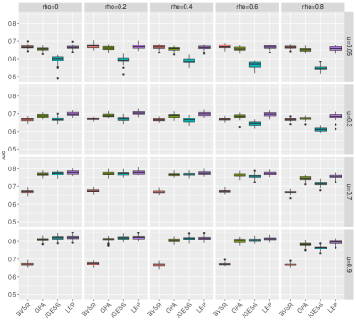
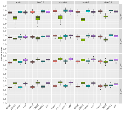
Figure 2: Comparison of BVSR, GPA, IGESS and Lasso with different $\{u,v\}$. Left panel: performance of risk variant identification measured by AUC; Right panel: performance of risk prediction. The number of summary-level datasets $K=1$. All the results are summarized based on 50 replications.

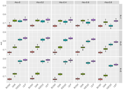
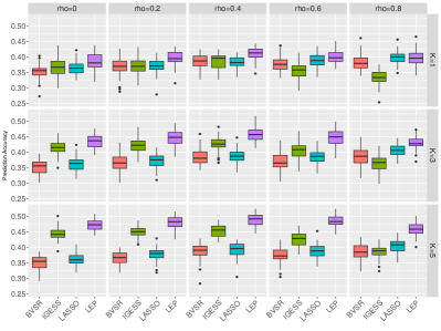
Figure 3: Comparison of BVSR, GPA, IGESS and Lasso with different $K$. Left panel: performance of risk variant identification measured by AUC; Right panel: performance of risk prediction. The indicator $u_{k}=0.5$ and sparsity-level $s=0.05$ . All the results are summarized based on 50 replications.

In this section, we conducted simulation studies to evaluate the performance of LEP in terms of both the risk variants identification and the risk prediction. The performance of the identification of risk variants was evaluated in comparison with BVSR (Carbonetto and Stephens, 2012), Lasso (Tibshirani, 1996) (only with individual-level data), IGESS (Dai et al., 2017) and GPA (Chung et al., 2014). Note that IGESS was based on a homogeneous assumption, i.e. $\Gamma_{j}^{1}$ = $\Gamma_{j}^{2}$ = …= $\Gamma_{jk}$ = $\gamma_{j}$, while GPA only worked for summary-statistics data. Then, the prediction accuracy of LEP was evaluated in comparison with BVSR, Lasso and IGESS. In the spirit of reproducibility, all the simulation codes were made publicly available at https://github.com/daviddaigithub/LEP.

3.1.1 Simulation settings

Both the individual-level and summary-level data were simulated in our experiments. In order to mimic the linkage disequilibrium (LD) of the individual-level data, the genotype matrix ${\mathbf{X}}$ was first generated by a zero-mean Gaussian distribution with a autoregressive structure for the co-variance matrix, where the autoregressive correlation $\rho^{|j-j^{\prime}|}$ indicated the correlation between the two corresponding variants. Clearly, $\rho=0$ corresponded to the situation that all the variants were independent. We considered $\rho=\{0,0.2,0.4,0.6,0.8\}$ in our simulations. Then each column of ${\mathbf{X}}$ was numerically coded as $\{0,1,2\}$ with probability $(1-f)^{2},2f(1-f)$ and $f^{2}$, respectively, according to Hardy-Weinberg principle, where $f$ was the minor allele frequency (MAF). We fixed the number of samples as $N=2,000$, the number of variants as $M=10,000$, and the sparsity-level $s=0.05$. On average, $M\cdot s$ nonzero entries in the vector of effect sizes $\bm{\beta}$ were generated using $N(0,1)$. The phenotype vector was generated as ${\mathbf{y}}={\mathbf{X}}\bm{\beta}+{\mathbf{e}}$, where the variance of ${\mathbf{e}}$ was adjusted such that heritability, i.e., $\mathrm{var}({\mathbf{X}}\bm{\beta})/\mathrm{var}({\mathbf{y}})$ was fixed at 50%.

The simulated $p$-values were obtained from the individual-level data instead of the generative model (Eq. (4)). Because the released summary-level data sets often have much larger sample sizes, we used $n_{0}=8,000$ samples to generate summary statistics, i.e., $p$-values in our simulation. We generated individual-level genotype data ${\mathbf{X}}^{(k)}$, as what we described above. To simulate the vector of effect size $\bm{\beta}^{(k)}$, we assume the $k$-th trait has the same of proportion of nonzero entries as the trait T, that is $s^{k}=s$. We generated the nonzero entries according to $(u_{k},v_{k})$ in Eq. (5) where $(u_{k},v_{k})$ satisfied $u_{k}s+(1-v_{k})(1-s)=s$, i.e., probability relationship,

$$\begin{split}\mathrm{Pr}(\Gamma_{jk}=1)=&\mathrm{Pr}(\Gamma_{jk}=1|\gamma_{j}=1)Pr(\gamma_{j}=1)\\ &+\mathrm{Pr}(\Gamma_{jk}=1|\gamma_{j}=0)Pr(\gamma_{j}=0).\end{split}$$

Again, the nonzero entries were drawn from $N(0,1)$, and the $k$-th phenotype vector was generated as ${\mathbf{y}}^{k}={\mathbf{X}}^{k}\bm{\beta}^{k}+{\mathbf{e}}_{k}$, where the variance of ${\mathbf{e}}_{k}$ was specified such that the heritability of the $k$-th phenotype was $50\%$. Then we obtained $p$-values of each variant by applying simple linear regression. To evaluate the performance of different methods, we pretended that we can not access the individual level data set but can only use the summary-level data, i.e. $p$-value matrix ${\mathbf{P}}\in\mathbb{R}^{M\times K}$.

For LEP and IGESS, both the individual-level data $\{{\mathbf{X}},{\mathbf{y}}\}$ and the $p$-value matrix ${\mathbf{P}}$ were used. For BVSR and Lasso, only the individual-level data set $\{{\mathbf{X}},{\mathbf{y}}\}$ was used, and their performance could serve as a baseline. For GPA, an $M\times 2$ matrix ${\mathbf{P}}$ containing the $p$-values from $\{{\mathbf{X}},{\mathbf{y}}\}$ and the $p$-values from the first study $\{{\mathbf{X}}^{(1)},{\mathbf{y}}^{(1)}\}$ was used as its input. We present the results of analyzing quantitative phenotype simulated as above in the main text and leave the results of case-control study in the Supplementary document.

3.1.2 Results

We conducted the comparisons in four scenarios and evaluated the performance of both risk variants identification and risk prediction. The performance of risk variants identification was measured by the area under the receiver operating characteristic (ROC) curve (AUC), and the performance of risk prediction was measured by the correlation between the observed phenotype values and the predicted values.

First, we fixed $K=1$, and varied $u$ at $\{0.9,0.7,0.3,0.05\}$ to mimic different pleiotropic settings to see the benefits of LEP. According to the condition of independence ($u$+$v$=$1$, see the detailed derivation in the Supplementary document), the parameter setting $u$ = 0.05 ($v$ = 0.95) corresponds to the situation that the trait of the summary-level data are irrelevant to the trait of the individual-level data. The pleiotropic effect between two traits increases as $u$ increases from $0.3$ to $0.9$. Fig. 2 shows the performance of risk variants identification and prediction under different pleiotropy settings. Here BVSR and Lasso using only individual-level data were used to serve as a baseline. In terms of risk variants identification, when the pleiotropic effect between two traits is high ($u$ = $\{0.7,0.9\}$), LEP, GPA and IGESS outperform BVSR working only with the individual-level dataset; when the pleiotropic effect is weak ($u=0.3$), LEP and GPA still perform better than BVSR. Moreover, when there is no relevant summary information ($u=0.05$), the performance of LEP is comparable to BVSR, which shows the robustness of LEP in the absence of useful summary information. It has similar results in terms of risk prediction. LEP and IGESS outperform BVSR and Lasso when the pleiotropic effect is high ($u$ = $\{0.7,0.9\}$). When the pleiotropic effect is weak ($u$ = $0.3$), LEP outperforms BVSR; When the summary-level data is irrelevant, LEP is slightly worse than Lasso, but is comparable with BVSR.

Second, we fixed $u_{k}:=\mathrm{Pr}(\Gamma_{jk}=1|\gamma_{j}=1)=0.5$, and varied the number of study with summary statistics at $K=\{1,3,5\}$ to see the improvements when more information was incorporated. Fig. 3 shows the improvement of LEP in comparisons with GPA, IGESS, BVSR and Lasso as $K$ increases. When $K=1$, GPA, IGESS and LEP all outperform BVSR as they use more information. LEP outperforms GPA as there is more useful information from the individual-level data. The performance of LEP increases as the number of $K$ increases. One can observe that IGESS has comparable performance to LEP but it can not control the FDR as shown in the Supplementary document. Instead, LEP is a method that could borrow strength from the study of a pleiotropic relationship and also control the FDR at the pre-specified level. All the results with respect to FDR, the power of risk variants identification are presented in the Supplementary document.

Last, we considered an extreme situation, the association status $\bm{\Gamma}_{\cdot k}$ (the $k$-th column of $\bm{\Gamma}$) was exactly the same as $\bm{\gamma}$, which was the assumption of IGESS, and the results are presented in the Supplementary document.

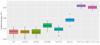
Figure 4: Prediction accuracy measured by AUC with different summary-level data. The plus sign ‘+’ means jointly analyzing CD and summary-level data for certain trait (s); T$\_$U$\_$P means jointly analyzing with T1D, UC and PBC; T$\_$U$\_$P$\_$A$\_$N means jointly analyzing with T1D, UC, PBC, AZ and NC. The results are based on 30 replications.

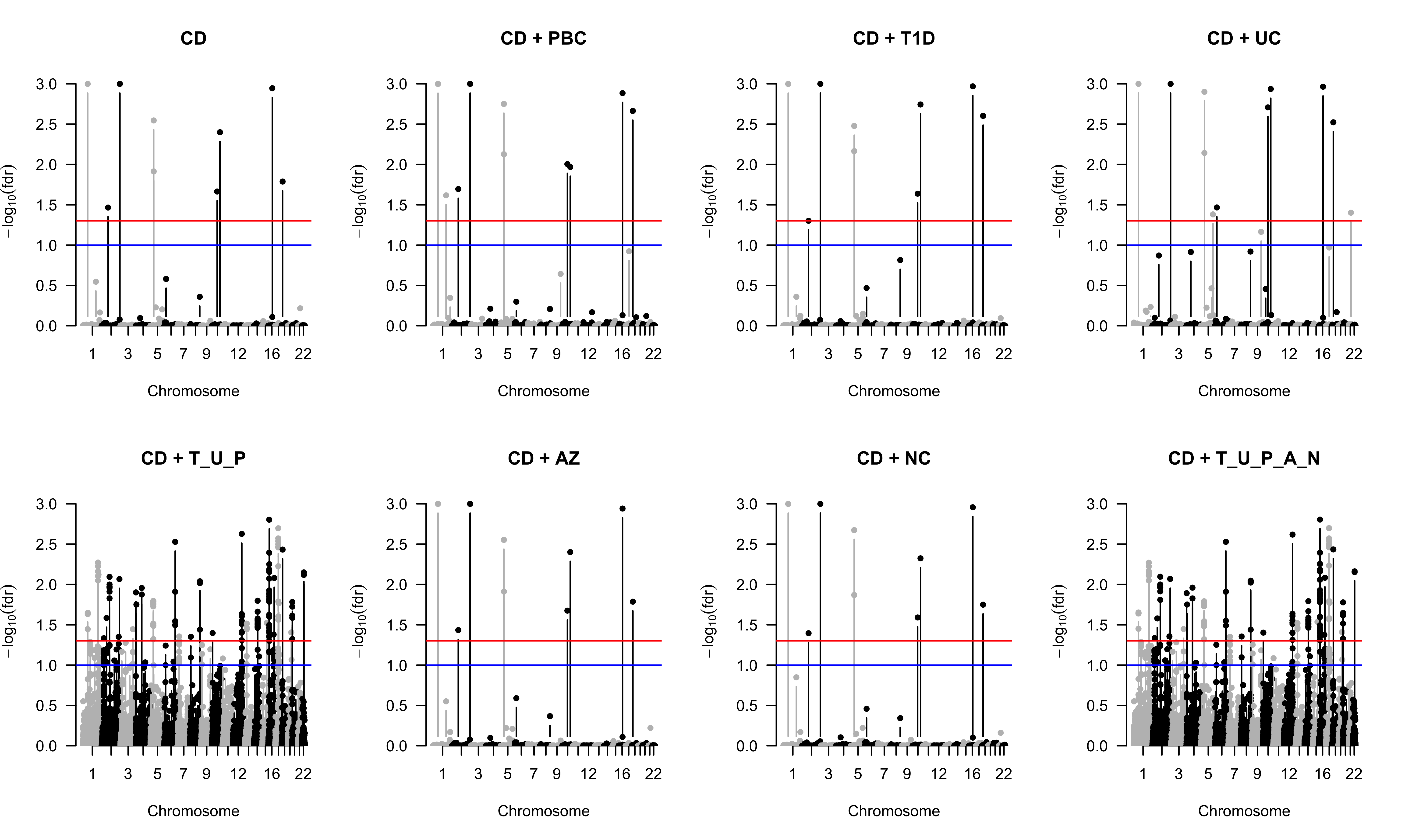
Figure 5: Manhattan plots of the analysis results of Crohn’s Disease using LEP. T$\_$U$\_$P means jointly analyzing with T1D, UC and PBC; T$\_$U$\_$P$\_$A$\_$N means jointly analyzing with T1D, UC, PBC, AZ and NC. The red lines and blue lines correspond to $fdr=0.05$ and $fdr=0.1$ respectively.

In summary, all the simulation results suggest that LEP is a reliable method when incorporating information from various kinds of summary statistics. It could make the most efficient use of the information as well as control the FDR well. Moreover, it will not degenerate the performance of analyzing individual-level data even when the summary statistics are from the irrelevant studies.

3.2 Real Data Analysis

We applied LEP to analyze GWAS data of Crohn’s disease (CD) with summary statistics from some other autoimmune diseases. The individual-level data is from the Welcome Trust Case Control Consortium (WTCCC) (Burton et al., 2007). There are 5,009 samples, of which 2,005 are cases and 3,004 are controls. The summary-level datasets are for Ulcerative colitis (UC), Primary biliary cirrhosis (PBC), Type 1 diabetes (T1D), three autoimmune-type diseases, are expected to be helpful in jointly analyzing with CD. In order to demonstrate the robustness of LEP on real data analysis, we selected two GWASs for Alzheimer (AZ), Neuroticism (NC), which were not relevant to CD by our common sense.

Table 1: Pleiotropy for the five data set with u,v

	GWAS	u	v
1	Ulcerative Colitis	1.0000	0.9260
2	Primary biliary cirrhosis	0.9998	0.9744
3	Type 1 diabetes	0.9986	0.9176
4	Alzheimer	2.72e-05	0.9325
5	Neuroticism	2.32e-03	0.7759

3.2.1 Quality Control on the individual-level data

The strict quality control (QC) on the individual-level data from WTCCC was performed by using PLINK (Purcell et al., 2007) and GCTA (Yang et al., 2011). First, we removed the individuals that has more than 2% missing genotypes; Before combining the CD dataset and the two control datasets, the SNPs with MAFs $<$ 0.05 and those with missing rate $>1\%$ were removed. Then we removed the SNPs with $p$-value $<0.0001$ in Hardy-Weinberg equilibrium test and kept one of the relatives with estimated relatedness $>0.025$ identified by GCTA (Yang et al., 2011) on the combined dataset. After QC, there were 1,656 cases and 2,880 controls remaining with 308,950 SNPs.

3.2.2 Summary-statistic data preprocessing

The details of the summary-level data were listed in Table S1 in Supplementary document. Taking overlapped SNPs among individual-level data and all the five phenotypes led to the individual-level data ${\mathbf{X}}\in\mathbb{R}^{N\times M},{\mathbf{y}}\in\mathbb{R}^{N\times 1}$ and a $p$-value matrix ${\mathbf{P}}\in\mathbb{R}^{M\times K}$ , where $N=4,536$, $M=194,782$ and $K=5$.

3.2.3 Analysis of pleiotropy with each single phenotype

We applied LEP to analyze the individual-level data for Crohn’s Disease with each of the five phenotypes. The results are listed in Table 1. The greater value of $u$ indicates a stronger pleiotropic relationship between the corresponding disease and the Crohn’s Disease. The values $\{u,v\}$ for Alzheimer and Neuroticism indicate that they almost share no associated variants with Crohn’s disease.

3.2.4 Analysis result of Crohn’s Disease

After analyzing the pleiotropy of each dataset with summary statistics, we then applied LEP to analyze CD with the selected summary statistics of PBC, T1D, UC, AZ and NC. The results for prediction accuracy and Manhattan plots of genome-wide hits are shown in Fig. 4 and Fig. 5, respectively.

The Manhattan plots in Fig. 5 indicate that it is more effective in identifying risk variants for CD by integrating the summary statistics from auto-immune diseases, i.e. UC, PBC and T1D, especially for combining them all. The irrelevant traits AZ, NC did not degenerate the performance of LEP in terms of identifying risk causal variants.

The results in Fig. 4 imply that the summary statistics of PBC, T1D and UC offer different degrees of relevant information, improving prediction accuracy (measured by AUC) from 63.39% ($\pm$0.58%) (only CD) to 65.66% ($\pm$0.44%) (with UC), and combining them all together could improve the prediction accuracy to 68.33% ($\pm$0.32%). These results suggested that information from diseases of a pleiotropic relationship could indeed substantially contribute to genetic prediction accuracy.

To demonstrate the robustness of LEP on the real data, we applied LEP on the individual-level data with each of them, their performance (63.34% ($\pm$0.53%), 63.40% ($\pm$0.54%)) was comparable with that of working on individual-level data alone (63.39% ($\pm$0.58%)). We also applied LEP with all the original summary statistics PBC, T1D, UC, AZ and NC, the performance slightly degraded from 68.33% ($\pm$0.32%) to 68.05% ($\pm$0.34%) suggesting the robustness of LEP when irrelevant summary-level datasets were included.

4 Conclusion

Restricted access to the individual-level data and the advantages of using summary-level data motivate the recent development of many new methods for further analyzing summary-level data. Working with the available but limited individual-level data and the abundant summary-level data is a promising direction to make the most efficient use of existing data resources. In this study, we propose a statistical approach, LEP, to integrating data at both the individual-level and summary-level, and the proposed method build a bridge from the individual-level data to summary-level data by modeling the pleiotropy. The implemented variational inference makes LEP scalable to genome-wide data analysis. The comprehensive simulations and real data analysis demonstrate the advantages of LEP and its wide applicabilities in practice. LEP will serve as a powerful tool for jointly analyzing individual-level data and summary statistics.

5 Appendix

5.1 Variational Expectation-Maximization Algorithm

5.1.1 E-Step

The joint probability for the LEP model could be rewritten as , let $\theta=\{\sigma^{2}_{\beta},\sigma^{2}_{e},\pi,\{\alpha_{k}\}_{k=1}^{K}\}$ be the collection of model parameters.

$${}\begin{split}&\mathrm{Pr}({\mathbf{y}},\tilde{\bm{\beta}},\bm{\gamma},\bm{\Gamma},{\mathbf{P}}|{\mathbf{X}};\bm{\theta})\\ =&\mathrm{Pr}({\mathbf{y}}|\tilde{\bm{\beta}},\bm{\gamma},{\mathbf{X}};\bm{\theta})\mathrm{Pr}(\tilde{\bm{\beta}};\bm{\theta})\mathrm{Pr}(\bm{\gamma}|\bm{\theta})\mathrm{Pr}(\mathbf{P}|\bm{\Gamma};\bm{\theta})\mathrm{Pr}(\bm{\Gamma}|\bm{\gamma}).\\ \end{split}$$ (15)

We model the relationship between $\gamma_{j}$ and $\Gamma_{jk}$ as

$$\begin{split}u_{k}:=\mathrm{Pr}(\Gamma_{jk}=1|\gamma_{j}=1),\\ v_{k}:=\mathrm{Pr}(\Gamma_{jk}=0|\gamma_{j}=0).\\ \end{split}$$ (16)

For the clarity of expression, we divide the joint probability into two parts, $\mathrm{Pr}({\mathbf{y}}|\tilde{\bm{\beta}},\bm{\gamma},{\mathbf{X}};\bm{\theta})\mathrm{Pr}(\tilde{\bm{\beta}};\bm{\theta})\mathrm{Pr}(\bm{\gamma}|\bm{\theta})$, for the individual-level data and $\mathrm{Pr}(\mathbf{P}|\bm{\Gamma};\bm{\theta})\mathrm{Pr}(\bm{\Gamma}|\bm{\gamma})$ for the summary-level data. We expanded them in the following form,

$$\mathrm{Pr}({\mathbf{y}}|\tilde{\bm{\beta}},\bm{\gamma},{\mathbf{X}};\bm{\theta})\mathrm{Pr}(\tilde{\bm{\beta}};\bm{\theta})\mathrm{Pr}(\bm{\gamma}|\bm{\theta})=N({\mathbf{y}}|\sum_{j}{\mathbf{x}}_{j}\tilde{\beta}_{j}\gamma_{j},\sigma^{2}_{e}\mathrm{I})\prod_{j=1}^{M}N(\tilde{\beta}_{j}|0,\sigma^{2}_{\beta})\pi^{\gamma_{j}}(1-\pi)^{1-\gamma_{j}}$$ (17)

and

$$\begin{split}\mathrm{Pr}(\mathbf{P}|\bm{\Gamma};\bm{\theta})\mathrm{Pr}(\bm{\Gamma}|\bm{\gamma})&=\prod_{j=1}^{M}\left(\prod_{k=1}^{K}\left(\mathrm{Pr}(p_{jk}|\Gamma_{jk}=1)\mathrm{Pr}(\Gamma_{jk}=1|\gamma_{j}=1)\right)^{\Gamma_{jk}}\left(\mathrm{Pr}(p_{jk}|\Gamma_{jk}=0)\mathrm{Pr}(\Gamma_{jk}=0|\gamma_{j}=1)\right)^{1-\Gamma_{jk}}\right)^{\gamma_{j}}\\ &\left(\prod_{k=1}^{K}\left(\mathrm{Pr}(p_{jk}|\Gamma_{jk}=1)\mathrm{Pr}(\Gamma_{jk}=1|\gamma_{j}=0)\right)^{\Gamma_{jk}}\left(\mathrm{Pr}(p_{jk}|\Gamma_{jk}=0)\mathrm{Pr}(\Gamma_{jk}=0|\gamma_{j}=0)\right)^{1-\Gamma_{jk}}\right)^{1-{\gamma_{j}}}\\ &=\prod_{j=1}^{M}\left(\prod_{k=1}^{K}(\alpha_{k}p_{jk}^{\alpha_{k}-1}u_{k})^{\Gamma_{jk}}(1-u_{k})^{1-\Gamma_{jk}}\right)^{\gamma_{j}}\left(\prod_{k=1}^{K}(\alpha_{k}p_{jk}^{\alpha_{k}-1}(1-v_{k}))^{\Gamma_{jk}}(v_{k})^{1-\Gamma_{jk}}\right)^{1-\gamma_{j}}.\\ \end{split}$$ (18)

The logarithm of the marginal likelihood is

$${}\begin{split}\log\mathrm{Pr}({\mathbf{y}},\mathbf{P}|{\mathbf{X}};\bm{\theta})&=\log\sum_{\bm{\gamma}}\sum_{\bm{\Gamma}}\int_{\tilde{\bm{\beta}}}\mathrm{Pr}({\mathbf{y}},\mathbf{P},\tilde{\bm{\beta}},\bm{\gamma},\bm{\Gamma}|{\mathbf{X}},\bm{\theta})d\tilde{\bm{\beta}}\\ &\geq\sum_{\bm{\gamma}}\sum_{\bm{\Gamma}}\int_{\tilde{\bm{\beta}}}q(\tilde{\bm{\beta}},\bm{\gamma},\bm{\Gamma})\log\frac{\mathrm{Pr}({\mathbf{y}},\tilde{\bm{\beta}},\mathbf{P},\bm{\gamma},\bm{\Gamma}|{\mathbf{X}},\bm{\theta})}{q(\tilde{\bm{\beta}},\bm{\gamma},\bm{\Gamma})}d\tilde{\bm{\beta}}\\ &=\mathbb{E}_{q}[\log\mathrm{Pr}({\mathbf{y}},\mathbf{P},\tilde{\bm{\beta}},\bm{\gamma},\bm{\Gamma}|{\mathbf{X}};\bm{\theta})-\log q(\tilde{\bm{\beta}},\bm{\gamma},\bm{\Gamma})]\\ &:=\mathcal{L}(q),\end{split}$$ (19)

where $\mathcal{L}(q)$ is the lower bound implied by Jensen’s inequality and the equality holds if and only if $q(\tilde{\bm{\beta}},\bm{\gamma},\bm{\Gamma})$ is the true posterior $\mathrm{Pr}(\tilde{\bm{\beta}},\bm{\gamma},\bm{\Gamma}|{\mathbf{y}},{\mathbf{P}},{\mathbf{X}};\bm{\theta})$. Instead of working with the marginal likelihood, we iteratively maximizing $\mathcal{L}(q)$. As it is stated in the main text, we employ the following variational distribution to make it feasible to evaluate the lower bound,

$$q(\tilde{\bm{\beta}},\bm{\gamma},\bm{\Gamma})=\prod_{j=1}^{M}q_{j}(\tilde{\bm{\beta}}_{j},\gamma_{j},\bm{\Gamma}_{j}),$$ (20)

where $\bm{\Gamma}_{j}=\{\Gamma_{j1},\ldots,\Gamma_{jK}\}$. According to the nice property of factorized distributions in variational inference, we can obtain the best approximation as

$${}\log q_{j}(\tilde{\beta}_{j},\gamma_{j},\bm{\Gamma}_{j})=\mathbb{E}_{i\neq j}[\log\mathrm{Pr}({\mathbf{y}},{\mathbf{P}},\tilde{\bm{\beta}},\bm{\gamma},\bm{\Gamma}|{\mathbf{X}};\bm{\theta})]+\mathrm{Const},$$ (21)

where the expectation is taken with respect to all of the other factors $\{q_{i}(\tilde{\beta}_{i},\gamma_{i},\bm{\Gamma}_{i})\}$ for $i\neq j$.

The logarithm of the joint probability function is

$${}\begin{split}\log\mathrm{Pr}({\mathbf{y}},{\mathbf{P}},\tilde{\bm{\beta}},\bm{\gamma},\bm{\Gamma}|{\mathbf{X}};\bm{\theta})&=-\frac{N}{2}\log(2\pi\sigma^{2}_{e})-\frac{{\mathbf{y}}^{T}{\mathbf{y}}}{2\sigma^{2}_{e}}\\ &\quad+\frac{\sum_{j=1}^{M}\gamma_{j}\tilde{\beta}_{j}{\mathbf{x}}^{T}_{j}{\mathbf{y}}}{\sigma^{2}_{e}}-\frac{1}{2\sigma^{2}_{e}}\sum_{j=1}^{M}\left((\gamma_{j}\tilde{\beta}_{j})^{2}{\mathbf{x}}_{j}^{T}{\mathbf{x}}_{j}\right)\\ &\quad-\frac{1}{2\sigma^{2}_{e}}\left(\sum_{j=1}^{M}\sum_{j^{\prime}\neq j}^{M}\gamma_{j}\tilde{\beta}_{j}\gamma_{j^{\prime}}\tilde{\beta}_{j^{\prime}}{\mathbf{x}}_{k}{\mathbf{x}}_{k}\right)\\ &\quad-\frac{M}{2}\log(2\pi\sigma^{2}_{\beta})-\frac{1}{2\sigma^{2}_{\beta}}\sum_{j=1}^{M}\tilde{\beta}_{j}^{2}\\ &\quad+\log\pi\sum_{j}\gamma_{j}+\log(1-\pi)\sum_{j}(1-\gamma_{j})\\ &+\sum_{j=1}^{M}\gamma_{j}\sum_{k=1}^{K}\Gamma_{jk}\log(\alpha_{k}p_{jk}^{\alpha_{k}-1}u_{k})+(1-\Gamma_{jk})\log(1-u_{k})\\ &+\sum_{j=1}^{M}(1-\gamma_{j})\sum_{k=1}^{K}\Gamma_{jk}\log(\alpha_{k}p_{jk}^{\alpha_{k}-1}(1-v_{k}))+(1-\Gamma_{jk})\log(v_{k}).\end{split}$$ (22)

Before proceeding, we should keep several things in our mind. First, $q(\tilde{\bm{\beta}},\bm{\gamma},\bm{\Gamma})$ is the variational approximation to the posterior $\mathrm{Pr}(\tilde{\bm{\beta}},\bm{\gamma},\bm{\Gamma}|{\mathbf{y}},{\mathbf{X}};\bm{\theta})$. Second, we assumed $q(\tilde{\bm{\beta}},\bm{\gamma},\bm{\Gamma})=\displaystyle\prod_{j=1}^{M}q(\tilde{\beta}_{j},\gamma_{j},\bm{\Gamma}_{j})$. Third, $q(\tilde{\beta}_{j},\gamma_{j},\bm{\Gamma}_{j})=q(\tilde{\beta}_{j}|\gamma_{j})q(\bm{\Gamma}_{j}|\gamma_{j})q(\gamma_{j})$.

To take the expectation in (21), we rearrange (22) into the terms with and without index $j$

$${}\begin{split}\log\mathrm{Pr}({\mathbf{y}},{\mathbf{P}},\tilde{\bm{\beta}},\bm{\gamma},\bm{\Gamma}|{\mathbf{X}};\bm{\theta})&=-\frac{N}{2}\log(2\pi\sigma^{2}_{e})-\frac{{\mathbf{y}}^{T}{\mathbf{y}}}{2\sigma^{2}_{e}}\\ &\quad+\frac{\gamma_{j}\tilde{\beta}_{j}{\mathbf{x}}^{T}_{j}{\mathbf{y}}}{\sigma^{2}_{e}}+\frac{\sum_{k\neq j}\gamma_{k}\tilde{\beta}_{k}{\mathbf{x}}^{T}_{j}{\mathbf{y}}}{\sigma^{2}_{e}}\\ &\quad-\frac{1}{2\sigma^{2}_{e}}\left((\gamma_{j}\tilde{\beta}_{j})^{2}{\mathbf{x}}^{T}_{j}{\mathbf{x}}_{j}\right)-\frac{1}{2\sigma^{2}_{e}}\sum_{k\neq j}\left((\gamma_{k}\tilde{\beta}_{k})^{2}{\mathbf{x}}^{T}_{k}{\mathbf{x}}_{k}\right)\\ &\quad-\frac{1}{\sigma^{2}_{e}}\left(\sum_{k\neq j}^{M}\gamma_{j}\tilde{\beta}_{j}\gamma_{k}\tilde{\beta}_{k}{\mathbf{x}}^{T}_{j}{\mathbf{x}}_{k}\right)-\frac{1}{2\sigma^{2}_{e}}\left(\sum_{k\neq j}\sum_{k^{\prime}\neq j}\gamma_{k}\tilde{\beta}_{k}\gamma_{k^{\prime}}\tilde{\beta}_{k^{\prime}}{\mathbf{x}}^{T}_{k}{\mathbf{x}}_{k^{\prime}}\right)\\ &\quad-\frac{M}{2}\log(2\pi\sigma^{2}_{\beta})-\frac{1}{2\sigma^{2}_{\beta}}\tilde{\beta}_{j}^{2}-\frac{1}{2\sigma^{2}_{\beta}}\sum_{k\neq j}\tilde{\beta}_{k}^{2}\\ &\quad+\log\pi\sum_{j}\gamma_{j}+\log(1-\pi)\sum_{j}(1-\gamma_{j})\\ &+\sum_{j=1}^{M}\gamma_{j}\sum_{k=1}^{K}\Gamma_{jk}\log(\alpha_{k}p_{jk}^{\alpha_{k}-1}u_{k})+(1-\Gamma_{jk})\log(1-u_{k})\\ &+\sum_{j=1}^{M}(1-\gamma_{j})\sum_{k=1}^{K}\Gamma_{jk}\log(\alpha_{k}p_{jk}^{\alpha_{k}-1}(1-v_{k}))+(1-\Gamma_{jk})\log(v_{k}).\end{split}$$ (23)

Because

$$\mathrm{Pr}(\Gamma_{jk}|p_{jk},\gamma_{j})=\frac{\mathrm{Pr}(p_{jk}|\Gamma_{jk})\mathrm{Pr}(\Gamma_{jk}|\gamma_{j})}{\mathrm{Pr}(p_{jk}|\Gamma_{jk}=1)\mathrm{Pr}(\Gamma_{jk}=1|\gamma_{j})+\mathrm{Pr}(p_{jk}|\Gamma_{jk}=0)\mathrm{Pr}(\Gamma_{jk}=0|\gamma_{j})},$$ (24)

we have

$$\begin{split}\mathrm{Pr}(\Gamma_{jk}=1|p_{jk},\gamma_{j}=1)&=\frac{\alpha_{k}p^{\alpha_{k}-1}_{jk}u_{k}}{\alpha_{k}p^{\alpha_{k}-1}_{jk}u_{k}+(1-u_{k})}=:q^{jk}_{11},\\ \mathrm{Pr}(\Gamma_{jk}=0|p_{jk},\gamma_{j}=1)&=\frac{1-u_{k}}{\alpha_{k}p^{\alpha_{k}-1}_{jk}u_{k}+(1-u_{k})}=:q^{jk}_{10},\\ \mathrm{Pr}(\Gamma_{jk}=1|p_{jk},\gamma_{j}=0)&=\frac{\alpha_{k}p^{\alpha_{k}-1}_{jk}(1-v_{k})}{\alpha_{k}p^{\alpha_{k}-1}_{jk}(1-v_{k})+v_{k}}=:q^{jk}_{01},\\ \mathrm{Pr}(\Gamma_{jk}=0|p_{jk},\gamma_{j}=0)&=\frac{v_{k}}{\alpha_{k}p^{\alpha_{k}-1}_{jk}(1-v_{k})+v_{k}}=:q^{jk}_{00}.\end{split}$$ (25)

Now we can take expectation of $\log\mathrm{Pr}({\mathbf{y}},\mathrm{P},\tilde{\bm{\beta}},\bm{\gamma},\bm{\Gamma}|{\mathbf{X}};\bm{\theta})$ under the distribution $q(\tilde{\beta}_{-j},\bm{\Gamma}_{-j.},\gamma_{-j}).$ When $\gamma_{j}=1$, we have

$$\log q(\tilde{\beta}_{j}|\gamma_{j}=1)=\left(-\frac{1}{2\sigma^{2}_{e}}{\mathbf{x}}^{T}_{j}{\mathbf{x}}_{j}-\frac{1}{2\sigma^{2}_{\beta}}\right)\tilde{\beta}^{2}_{j}+\frac{{\mathbf{x}}^{T}_{j}{\mathbf{y}}-\displaystyle\sum_{k\neq j}^{M}\mathbb{E}_{k}[\gamma_{k}\tilde{\beta}_{k}]{\mathbf{x}}^{T}_{j}{\mathbf{x}}_{k}}{\sigma^{2}_{e}}\tilde{\beta}_{j}+\mathrm{Const}$$ (26)

and

$$q(\Gamma_{jk}|\gamma_{j}=1)=(q_{11}^{jk})^{\Gamma_{jk}}(q^{jk}_{10})^{1-\Gamma_{jk}}.$$ (27)

Because $\log q(\tilde{\beta}_{j}|\gamma_{j}=1)$ is a quadratic form, we know $q(\beta_{j}|\gamma_{j}=1)=N(\beta_{j}|\mu_{j},s^{2}_{j})$, where

$${}\begin{split}s^{2}_{j}&=\frac{\sigma^{2}_{e}}{{\mathbf{x}}^{T}_{j}{\mathbf{x}}_{j}+\frac{\sigma^{2}_{e}}{\sigma^{2}_{\beta}}},\\ \mu_{j}&=\frac{{\mathbf{x}}^{T}_{j}{\mathbf{y}}-\sum_{k\neq j}\mathbb{E}_{k}[\gamma_{k}\beta_{k}]{\mathbf{x}}^{T}_{j}{\mathbf{x}}_{k}}{{\mathbf{x}}^{T}_{j}{\mathbf{x}}_{j}+\frac{\sigma^{2}_{e}}{\sigma^{2}_{\beta}}}.\end{split}$$ (28)

Similarly, when $\gamma_{j}=0$, we have

$$\log q(\tilde{\beta}_{j}|\gamma_{j}=0)=-\frac{1}{2\sigma^{2}_{\beta}}\tilde{\beta}^{2}_{j}+\mathrm{Const}$$ (29)

and

$$q(\Gamma_{jk}|\gamma_{j}=0)=(q_{01}^{jk})^{\Gamma_{jk}}(q^{jk}_{00})^{1-\Gamma_{jk}}.$$ (30)

According to Eq. (29), we know $q(\tilde{\beta}_{j}|\gamma_{j}=0)=N(\tilde{\beta}_{j}|0,\sigma^{2}_{\beta})$. This is a very good property as it says that the posterior distribution of $\tilde{\beta}_{j}$ will be the same as its prior if this variable is irrelevant ( $\gamma_{j}=0$ ). Note that $\gamma_{j}$ is a binary variable and then denote $\pi_{j}=q(\gamma_{j}=1).$ Therefore we have

$$q(\tilde{\beta}_{j},\gamma_{j},\bm{\Gamma}_{j})=\left(\pi_{j}N(\mu_{j},s^{2}_{j})\prod_{k=1}^{K}q(\Gamma_{jk}|r_{j}=1)\right)^{\gamma_{j}}\left((1-\pi_{j})N(0,\sigma^{2}_{\beta})\prod_{k=1}^{K}q(\Gamma_{jk}|r_{j}=0)\right)^{1-\gamma_{j}}.$$ (31)

Now we evaluate the variational lower bound $\mathcal{L}(q)$ (19).

$$\begin{split}\mathcal{L}(q)=\mathbb{E}_{q}[\log\mathrm{Pr}({\mathbf{y}},\mathbf{P},\tilde{\bm{\beta}},\bm{\gamma},\bm{\Gamma}|{\mathbf{X}};\bm{\theta})]-\mathbb{E}_{q}[\log q(\tilde{\bm{\beta}},\bm{\gamma},\bm{\Gamma})].\\ \end{split}$$ (32)

The first part of Eq. (32) could be written as

$$\begin{split}&\quad\mathbb{E}_{q}[\log\mathrm{Pr}({\mathbf{y}},\mathbf{P},\tilde{\bm{\beta}},\bm{\gamma},\bm{\Gamma}|{\mathbf{X}};\theta)]\\ &=-\frac{N}{2}\log(2\pi\sigma^{2}_{e})-\frac{{\mathbf{y}}^{T}{\mathbf{y}}}{2\sigma^{2}_{e}}\\ &+\frac{\displaystyle\sum_{j=1}^{M}\mathbb{E}[\gamma_{j}\tilde{\beta}_{j}]{\mathbf{x}}^{T}_{j}{\mathbf{y}}}{\sigma^{2}_{e}}\\ &-\frac{1}{2\sigma^{2}_{e}}\sum_{j=1}^{M}\left(\mathbb{E}[(\gamma_{j}\tilde{\beta}_{j})^{2}]{\mathbf{x}}^{T}_{j}{\mathbf{x}}_{j}\right)\\ &-\frac{1}{2\sigma^{2}_{e}}\left(\sum_{j=1}^{M}\sum_{j^{\prime}\neq j}^{M}\mathbb{E}[\gamma_{j}\tilde{\beta}_{j}]\mathbb{E}[\gamma_{j^{\prime}}\tilde{\beta}_{j^{\prime}}]{\mathbf{x}}^{T}_{j}{\mathbf{x}}_{j^{\prime}}\right)\\ &-\frac{M}{2}\log(2\pi\sigma^{2}_{\beta})-\frac{1}{2\sigma^{2}_{\beta}}\sum_{j=1}^{M}\mathbb{E}[\tilde{\beta}_{j}^{2}]\\ &+\log\pi\sum_{j}\mathbb{E}[\gamma_{j}]+\log(1-\pi)\sum_{j}\mathbb{E}[1-\gamma_{j}]\\ &+\sum_{j=1}^{M}\pi_{j}\sum_{k=1}^{K}q_{11}^{k}(\log(\alpha_{k}p_{jk}^{\alpha_{k}-1}u_{k}))+q_{10}^{k}\log(1-u_{k})\\ &+\sum_{j=1}^{M}(1-\pi_{j})\sum_{k=1}^{K}q_{01}^{k}(\log(\alpha_{k}p_{jk}^{\alpha_{k}-1}(1-v_{k}))+q_{00}^{k}\log(v_{k}).\end{split}$$ (33)

Because $q(\tilde{\bm{\beta}},\bm{\gamma},\bm{\Gamma})=q(\tilde{\bm{\beta}}|\bm{\gamma})q(\bm{\gamma})q(\bm{\Gamma}|\bm{\gamma})$, the second term of Eq. (32) could be written as

$$-\mathbb{E}_{q}[\log q(\tilde{\bm{\beta}},\bm{\gamma},\bm{\Gamma})]=-\mathbb{E}_{q}[\log q(\tilde{\bm{\beta}},\bm{\gamma})]-\mathbb{E}_{q}[\log q(\bm{\Gamma}|\bm{\gamma})].$$ (34)

The two terms of Eq. (34) could be evaluated respectively, we have

$$\begin{split}-\mathbb{E}_{q}[\log q(\tilde{\bm{\beta}},\bm{\gamma})]&=\frac{M}{2}\log\sigma^{2}_{\beta}+\sum_{j}\frac{1}{2}\pi_{j}(\log s^{2}_{j}-\log\sigma^{2}_{\beta})\\ &\quad-\sum_{j}(\pi_{j}\log\pi_{j}+(1-\pi_{j})\log(1-\pi_{j}))\\ \end{split}$$ (35)

and

$$\begin{split}q(\bm{\Gamma}|\gamma)&=\prod_{j=1}^{M}\left(\prod_{k=1}^{K}\left(\frac{\alpha_{k}p^{\alpha_{k}-1}_{jk}u_{k}}{\alpha_{k}p^{\alpha_{k}-1}_{jk}u_{k}+(1-u_{k})}\right)^{\Gamma_{jk}}\left(\frac{1-u_{k}}{\alpha_{k}p^{\alpha_{k}-1}_{jk}u_{k}+(1-u_{k})}\right)^{1-\Gamma_{jk}}\right)^{\gamma_{j}}\\ &\left(\prod_{k=1}^{K}\left(\frac{\alpha_{k}p^{\alpha_{k}-1}_{jk}(1-v_{k})}{\alpha_{k}p^{\alpha_{k}-1}_{jk}(1-v_{k})+v_{k}}\right)^{\Gamma_{jk}}\left(\frac{v_{k}}{\alpha_{k}p^{\alpha_{k}-1}_{jk}(1-v_{k})+v_{k}}\right)^{1-\Gamma_{jk}}\right)^{1-\gamma_{j}}\\ &=\prod_{j=1}^{M}\left(\prod_{k=1}^{K}(q^{jk}_{11})^{\Gamma_{jk}}(q^{jk}_{10})^{1-\Gamma_{jk}}\right)^{\gamma_{j}}\left(\prod_{k=1}^{K}(q^{jk}_{01})^{\Gamma_{jk}}(q^{jk}_{00})^{1-\Gamma_{jk}}\right)^{1-\gamma_{j}},\\ \end{split}$$ (36)

then

$$-\mathbb{E}_{q}[\log q(\bm{\Gamma}|\gamma)]=-\left(\sum_{j=1}^{M}\pi_{j}\left(\sum_{k=1}^{K}q_{11}^{jk}\log q^{jk}_{11}+q_{10}^{jk}\log q^{jk}_{10}\right)+(1-\pi_{j})\left(\sum_{k=1}^{K}q_{01}^{jk}\log q^{jk}_{01}+q_{00}^{jk}\log q^{jk}_{00}\right)\right).$$ (37)

Now we substitute $\mathbb{E}[\gamma_{j}\tilde{\beta}_{j}]=\pi_{j}\mu_{j}$, $\mathbb{E}[(\gamma_{j}\tilde{\beta}_{j})^{2}]=\pi_{j}(s^{2}_{j}+\mu^{2}_{j})$, $\mathbb{E}[\tilde{\beta}_{j}^{2}]=\pi_{j}(s^{2}_{j}+\mu^{2}_{j})+(1-\pi_{j})\sigma^{2}_{\beta}$, $\mathbb{E}[\gamma_{j}]=\pi_{j}$ and $\mathbb{E}[1-\gamma_{j}]=1-\pi_{j}.$

We rearrange the lower bound

$$\begin{split}\mathcal{L}(q)&=\mathbb{E}_{q}[\log\mathrm{Pr}({\mathbf{y}},{\mathbf{P}},\tilde{\bm{\beta}},\bm{\gamma}|{\mathbf{X}},\theta)]-\mathbb{E}_{q}[\log q(\tilde{\bm{\beta}},\bm{\gamma},\bm{\Gamma})]\\ &=-\frac{N}{2}\log(2\pi\sigma^{2}_{e})-\frac{\|{\mathbf{y}}-\sum_{j}\pi_{j}\mu_{j}{\mathbf{x}}_{j}\|^{2}}{2\sigma^{2}_{e}}-\frac{1}{2\sigma^{2}_{e}}\sum_{j=1}^{M}[\pi_{j}(s^{2}_{j}+\mu^{2}_{j})-(\pi_{j}\mu_{j})^{2}]{\mathbf{x}}^{T}_{j}{\mathbf{x}}_{j}\\ &\quad-\frac{M}{2}\log(2\mathrm{\pi})-\frac{1}{2\sigma^{2}_{\beta}}\sum_{j=1}^{M}[\pi_{j}(\mu^{2}_{j}+s^{2}_{j})+(1-\pi_{j})\sigma^{2}_{\beta}]\\ &\quad+\sum_{j}\pi_{j}\log(\frac{\pi}{\pi_{j}})+\sum_{j}(1-\pi_{j})\log(\frac{1-\pi}{1-\pi_{j}})\\ &\quad+\sum_{j}\frac{1}{2}\pi_{j}(\log s^{2}_{j}-\log\sigma^{2}_{\beta})\\ &+\sum_{j=1}^{M}\pi_{j}\sum_{k=1}^{K}q_{11}^{jk}\log(\alpha_{k}p_{jk}^{\alpha_{k}-1}u_{k})+q_{10}^{jk}\log(1-u_{k})\\ &+\sum_{j=1}^{M}(1-\pi_{j})\sum_{k=1}^{K}q_{01}^{jk}(\log(\alpha_{k}p_{jk}^{\alpha_{k}-1}(1-v_{k}))+q_{00}^{jk}\log(v_{k})\\ &-\left(\sum_{j=1}^{M}\pi_{j}\left(\sum_{k=1}^{K}q_{11}^{jk}\log q^{jk}_{11}+q_{10}^{jk}\log q^{jk}_{10}\right)+(1-\pi_{j})\left(\sum_{k=1}^{K}q_{01}^{jk}\log q^{jk}_{01}+q_{00}^{jk}\log q^{jk}_{00}\right)\right),\\ \end{split}$$ (38)

simplifying the last three rows of Eq. (38), we could get the following equation,

$$\begin{split}&\sum_{j=1}^{M}\pi_{j}\sum_{k=1}^{K}q_{11}^{jk}\log(\alpha_{k}p_{jk}^{\alpha_{k}-1}u_{k})+q_{10}^{jk}\log(1-u_{k})\\ &+\sum_{j=1}^{M}(1-\pi_{j})\sum_{k=1}^{K}q_{01}^{jk}(\log(\alpha_{k}p_{jk}^{\alpha_{k}-1}(1-v_{k}))+q_{00}^{jk}\log(v_{k})\\ &-\left(\sum_{j=1}^{M}\pi_{j}\left(\sum_{k=1}^{K}q_{11}^{jk}\log q^{jk}_{11}+q_{10}^{jk}\log q^{jk}_{10}\right)+(1-\pi_{j})\left(\sum_{k=1}^{K}q_{01}^{jk}\log q^{jk}_{01}+q_{00}^{jk}\log q^{jk}_{00}\right)\right)\\ &=\sum_{j=1}^{M}\pi_{j}\sum_{k=1}^{K}\log(\alpha_{k}p_{jk}^{\alpha_{k}-1}u_{k}+1-u_{k})+\sum_{j=1}^{M}(1-\pi_{j})\sum_{k=1}^{K}\log(\alpha_{k}p_{jk}^{\alpha_{k}-1}(1-v_{k})+v_{k}).\end{split}$$ (39)

To get $\pi_{j}$, we set $\frac{\partial\mathcal{L}(q)}{\partial\pi_{j}}=0$, yielding

$$\pi_{j}=\frac{1}{1+\exp(-w_{j})},\mathrm{where}~{}w_{j}=\log\frac{\pi}{1-\pi}+\frac{1}{2}\log\frac{s^{2}_{j}}{\sigma^{2}_{\beta}}+\frac{\mu_{j}^{2}}{2s^{2}_{j}}+\sum_{k=1}^{K}\log\frac{\alpha_{k}p_{jk}^{\alpha_{k}-1}u_{k}+1-u_{k}}{\alpha_{k}p_{jk}^{\alpha_{k}-1}(1-v_{k})+v_{k}}.$$ (40)

5.1.2 M-Step

We will update the model parameters $\bm{\theta}=\{\sigma^{2}_{\beta},\sigma^{2}_{e},\pi,\{\alpha_{k}\}_{k=1}^{K}\}$ sequentially by maximizing the lower bound $\mathcal{L}(q)$.
To get $\sigma^{2}_{\beta}$, we set

$$\begin{split}\frac{\partial\mathcal{L}(q)}{\partial\sigma^{2}_{\beta}}&=\frac{\partial\mathbb{E}_{q}[\log\mathrm{Pr}({\mathbf{y}},\tilde{\bm{\beta}},\bm{\gamma},{\mathbf{P}}|{\mathbf{X}},\bm{\theta})]}{\partial\sigma^{2}_{\beta}}=0,\\ \end{split}$$ (41)

yielding

$$\sigma^{2}_{\beta}=\frac{\sum_{j}\pi_{j}(\mu^{2}_{j}+s^{2}_{j})}{\sum_{j}\pi_{j}}.$$ (42)

To get $\sigma^{2}_{e}$, we set

$$\begin{split}\frac{\partial\mathcal{L}(q)}{\partial\sigma^{2}_{e}}=\frac{\partial\mathbb{E}_{q}[\log\mathrm{Pr}({\mathbf{y}},\tilde{\bm{\beta}},\bm{\gamma},{\mathbf{P}}|{\mathbf{X}},\bm{\theta})]}{\partial\sigma^{2}_{e}}&=-\frac{N}{2}\frac{1}{\sigma^{2}_{e}}+\frac{{\mathbf{y}}^{T}{\mathbf{y}}}{2\sigma^{4}_{e}}\\ &-\frac{\sum_{j}\mathbb{E}[\gamma_{j}\tilde{\beta}_{j}]{\mathbf{x}}^{T}_{j}{\mathbf{y}}}{\sigma^{4}_{e}}\\ &+\frac{1}{2\sigma^{4}_{e}}\sum_{j=1}^{M}(\mathbb{E}[(\gamma_{j}\tilde{\beta}_{j})^{2}]{\mathbf{x}}^{T}_{j}{\mathbf{x}}_{j})\\ &+\frac{1}{2\sigma^{4}_{e}}\left(\sum_{j=1}^{M}\sum_{j^{\prime}\neq j}^{M}\mathbb{E}[\gamma_{j}\tilde{\beta}_{j}]\mathbb{E}[\gamma_{j^{\prime}}\tilde{\beta}_{j^{\prime}}]{\mathbf{x}}^{T}_{j}{\mathbf{x}}_{j^{\prime}}\right)=0,\end{split}$$ (43)

yielding

$$\begin{split}\sigma^{2}_{e}&=\frac{1}{N}\left({\mathbf{y}}^{T}{\mathbf{y}}-2\sum_{j}\mathbb{E}[\gamma_{j}\tilde{\beta}_{j}]{\mathbf{x}}^{T}_{j}{\mathbf{y}}+\sum_{j=1}^{M}(\mathbb{E}[(\gamma_{j}\tilde{\beta}_{j})^{2}]{\mathbf{x}}^{T}_{j}{\mathbf{x}}_{j})+\sum_{j=1}^{M}\sum_{j^{\prime}\neq j}^{M}\mathbb{E}[\gamma_{j}\tilde{\beta}_{j}]\mathbb{E}[\gamma_{j^{\prime}}\tilde{\beta}_{j^{\prime}}]{\mathbf{x}}^{T}_{j}{\mathbf{x}}_{j^{\prime}}\right)\\ &=\frac{1}{N}\left({\mathbf{y}}^{T}{\mathbf{y}}-2\sum_{j}\mathbb{E}[\gamma_{j}\tilde{\beta}_{j}]{\mathbf{x}}^{T}_{j}{\mathbf{y}}+\sum_{j=1}^{M}\sum_{j^{\prime}=1}^{M}\mathbb{E}[\gamma_{j}\tilde{\beta}_{j}]\mathbb{E}[\gamma_{j^{\prime}}\tilde{\beta}_{j^{\prime}}]{\mathbf{x}}^{T}_{j}{\mathbf{x}}_{j^{\prime}}+\sum_{j=1}^{M}(\mathbb{E}[(\gamma_{j}\tilde{\beta}_{j})^{2}]{\mathbf{x}}^{T}_{j}{\mathbf{x}}_{j})-\sum_{j=1}^{M}(\mathbb{E}[\gamma_{j}\tilde{\beta}_{j}])^{2}{\mathbf{x}}_{j}^{T}{\mathbf{x}}_{j}\right)\\ &=\frac{1}{N}\left(\|{\mathbf{y}}-\sum_{j}\pi_{j}\mu_{j}{\mathbf{x}}_{j}\|^{2}+\sum_{j=1}^{M}(\pi_{j}(s_{j}^{2}+\mu_{j}^{2})-(\pi_{j}\mu_{j})^{2}){\mathbf{x}}_{j}^{T}{\mathbf{x}}_{j}\right).\end{split}$$ (44)

To get $\pi$, we set $\frac{\partial\mathcal{L}(q)}{\partial\pi}=0$, yielding

$$\pi=\frac{1}{M}\sum_{j}\pi_{j}.$$ (45)

The parameter of the beta distribution, $\alpha_{k}$, could be obtained by maximizing $\mathcal{L}(q)$,

$$\alpha_{k}=\frac{\displaystyle\sum_{j=1}^{M}\pi_{j}q^{jk}_{11}+(1-\pi_{j})q^{jk}_{01}}{\displaystyle\sum_{j=1}^{M}\left(\pi_{j}q^{jk}_{11}+(1-\pi_{j})q^{jk}_{01}\right)(-\log(p_{jk}))}.$$ (46)

The parameters $u_{k}$ and $v_{k}$ could also be obtained by maximizing $\mathcal{L}(q)$, we have

$$u_{k}=\frac{\sum_{j=1}^{M}\pi_{j}q^{jk}_{11}}{\sum_{j=1}^{M}\pi_{j}},$$ (47)

$$v_{k}=\frac{\sum_{j=1}^{M}(1-\pi_{j})q^{jk}_{00}}{\sum_{j=1}^{M}(1-\pi_{j})}.$$ (48)

5.2 ALGORITHMS

5.2.1 Basic Algorithm Steps

Now we describe an algorithm:

• $\mathrm{Initialize}$ $\{\pi_{j},\mu_{j}\}_{j=1}^{M},\sigma^{2}_{\beta},\sigma^{2}_{e},\{\alpha_{k}\}_{k=1}^{K},\{q_{00}^{jk}\},\{q_{11}^{jk}\}$. Let $\tilde{{\mathbf{y}}}=\sum_{j}\pi_{j}\mu_{j}{\mathbf{x}}_{j}.$

• $\mathrm{E-Step}$: For $j=1,\ldots,M$, first obtain

  $${}\tilde{{\mathbf{y}}}_{j}=\tilde{{\mathbf{y}}}-\pi_{j}\mu_{j}{\mathbf{x}}_{j},$$ (49)

  and then update $\mu_{j},s^{2}_{j},\pi_{j}$ and $\tilde{{\mathbf{y}}}$ as follows

  $$s^{2}_{j} =\frac{\sigma^{2}_{e}}{{\mathbf{x}}^{T}_{j}{\mathbf{x}}_{j}+\sigma^{2}_{e}/\sigma^{2}_{\beta}},$$ (50)

  $$\mu_{j} =\frac{{\mathbf{x}}^{T}_{j}({\mathbf{y}}-\tilde{{\mathbf{y}}}_{j})}{{\mathbf{x}}^{T}_{j}{\mathbf{x}}_{j}+\sigma^{2}_{e}/\sigma^{2}_{\beta}},$$ (51)

  $$\pi_{j} =\frac{1}{1+\exp(-w_{j})},\mathrm{where}~{}w_{j}=\log\frac{\pi}{1-\pi}+\frac{1}{2}\log\frac{s^{2}_{j}}{\sigma^{2}_{\beta}}+\frac{\mu_{j}^{2}}{2s^{2}_{j}}+\sum_{k=1}^{K}\log\frac{\alpha_{k}p_{jk}^{\alpha_{k}-1}u_{k}+1-u_{k}}{\alpha_{k}p_{jk}^{\alpha_{k}-1}(1-v_{k})+v_{k}},$$ (52)

  $$\tilde{{\mathbf{y}}} =\tilde{{\mathbf{y}}}_{j}+\pi_{j}\mu_{j}{\mathbf{x}}_{j}.$$ (53)

• $\mathrm{M-Step}$

  $$\begin{split}\sigma^{2}_{e}&=\left(\|{\mathbf{y}}-\tilde{{\mathbf{y}}}\|^{2}+\sum_{j=1}^{M}(\pi_{j}(s_{j}^{2}+\mu_{j}^{2})-(\pi_{j}\mu_{j})^{2}){\mathbf{x}}_{j}^{T}{\mathbf{x}}_{j}\right)/N,\\ \alpha_{k}&=\frac{\displaystyle\sum_{j=1}^{M}\pi_{j}q^{jk}_{11}+(1-\pi_{j})q^{jk}_{01}}{\displaystyle\sum_{j=1}^{M}\left(\pi_{j}q^{jk}_{11}+(1-\pi_{j})q^{jk}_{01}\right)(-\log(p_{jk}))},\\ u_{k}&=\frac{\sum_{j=1}^{M}\pi_{j}q^{jk}_{11}}{\sum_{j=1}^{M}\pi_{j}},\\ v_{k}&=\frac{\sum_{j=1}^{M}(1-\pi_{j})q^{jk}_{00}}{\sum_{j=1}^{M}(1-\pi_{j})},\\ \sigma^{2}_{\beta}&=\frac{\sum_{j}\pi_{j}(\mu_{j}^{2}+s^{2}_{j})}{\sum_{j}\pi_{j}},\\ \pi&=\frac{1}{M}\sum_{j}\alpha_{j}.\end{split}$$ (54)

• Evaluate the lower bound $\mathcal{L}(q)$, check the stop criteria.

According to the definition, we could update $q_{11}^{jk},q_{00}^{jk}$ by

$$\begin{split}q^{jk}_{11}&=\frac{\alpha_{k}p^{\alpha_{k}-1}_{jk}u_{k}}{\alpha_{k}p^{\alpha_{k}-1}_{jk}u_{k}+(1-u_{k})},\\ q^{jk}_{00}&=\frac{v_{k}}{\alpha_{k}p^{\alpha_{k}-1}_{jk}(1-v_{k})+v_{k}}.\end{split}$$ (55)

5.3 Condition of irrelevance between the individual-level data and summary-level data

If the association status for the individual-level data and the $k$-th trait are irrelevant, the following equation holds,

$$\Pr(\gamma_{j}=1,\Gamma_{jk}=1)=\Pr(\gamma_{j}=1)\Pr(\Gamma_{jk}=1).$$ (56)

As defined in the main text, $s=\mathrm{Pr}(\gamma_{j}=1),u_{k}=\Pr(\Gamma_{jk}=1|\gamma_{j}=1)$, the left side of Eq.(56) could be written as

$$\Pr(\gamma_{j}=1,\Gamma_{jk}=1)=\Pr(\Gamma_{jk}=1|\gamma_{j}=1)\mathrm{Pr}(\gamma_{j}=1)=u_{k}s.$$ (57)

As

$$\begin{split}\mathrm{Pr}(\Gamma_{jk}=1)&=\mathrm{Pr}(\Gamma_{jk}=1|\gamma_{j}=1)\mathrm{Pr}(\gamma_{j}=1)+\mathrm{Pr}(\Gamma_{jk}=1|\gamma_{j}=0)\mathrm{Pr}(\gamma_{j}=0)\\ &=u_{k}s+(1-v_{k})(1-s),\end{split}$$ (58)

When Eq.(56) holds, we have

$$u_{k}s=s(u_{k}s+(1-v_{k})(1-s)).$$ (59)

We could easily get the irrelevant condition for the $k$-th trait with Trait T as

$$u_{k}+v_{k}=1.$$ (60)

5.4 MORE RESULTS IN THE SIMULATION EXPERIMENTS

In this section, we present more simulation results to the demonstrate the effectiveness of LEP. The results contains four parts, (1) Performance of FDR control under different pleiotropy settings; (2) Performance of FDR control with different number of summary-level datasets; (3) Performance of risk variant identification and risk prediction under homogeneous assumption; (4) The results for the case-control studies. As in the main text, the number of samples and the number of variants were set to be $N=2,000$ and $M=10,000$, respectively. The heritability was pre-specified at 0.5 with the sparsity-level $s=0.05$.

5.4.1 Performance of FDR control under different pleiotropy settings

In the main text, we have compared LEP with BVSR, GPA and IGESS in terms of risk variants identification (AUC) and risk prediction under different pleiotropy settings (varying $u$ at 0.05, 0.3, 0.7, 0.9), in this sub section, we list the results of FDR (False Discovery Rate) control. All the datasets in this sub section are simulated under different LD setting, $\rho=\{0,0.2,0.4,0.6,0.8\}$, and the results are based on 50 replications.

As the results shown Fig. 6, LEP could control FDR well with small or moderate LD as $\rho=\{0.2,0.4,0.6\}$, we have observed slightly inflated FDR when $\rho=0.8$.

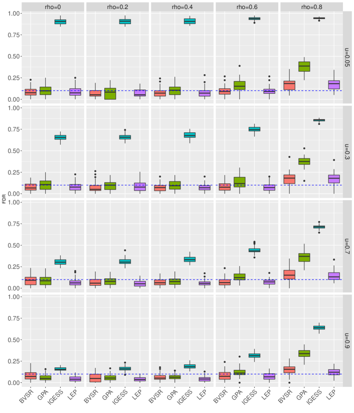
Figure 6: Performance of False Discovery Rate (FDR) Control at pre-specified level FDR$=0.1$ under different pleiotropy settings and different LD. $K=1$.

5.4.2 Performance of FDR control with different number of summary-level datasets

In the main text, we have compared LEP with BVSR, GPA and IGESS in terms of variants risk identification(AUC) and risk prediction with different number of summary-level datasets, in this sub section, we evaluate the performance of FDR control.

According to the results in Fig. 7, LEP could also control the FDR at the pre-specified level FDR=$0.1$ when $\rho=\{0,0.2,0.4,0.6\}$. We have observed slightly inflated FDR when $\rho=0.8$.

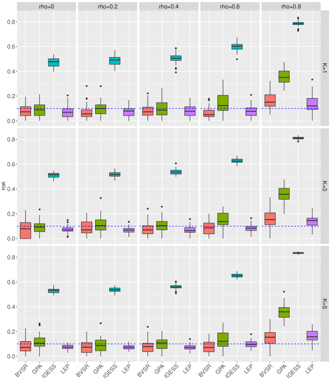
Figure 7: Performance of False Discovery Rate (FDR) Control at pre-specified level $FDR=0.1$ under different pleiotropy settings and different LD. Here $u=0.5$

5.4.3 Results for the homogeneous assumption

We considered an extreme situation with a homogeneous assumption (the assumption of IGESS), $\Gamma_{j1}=\ldots=\Gamma_{jK}=\bm{\Gamma}_{j}$, according to the results in Fig. 8, we could see LEP has comparable performance with IGESS, LEP and IGESS all outperform BVSR and Lasso as they take in more information in the analysis effectively.

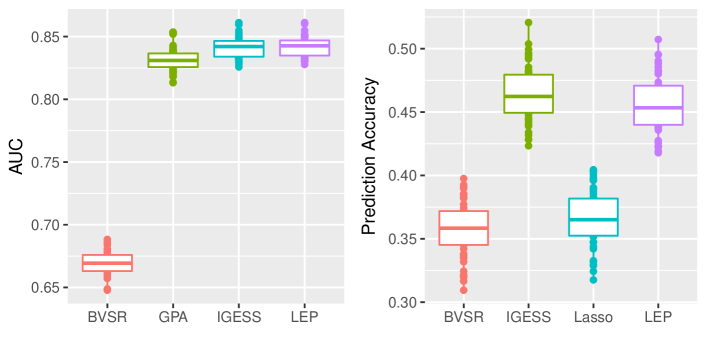
Figure 8: Comparison of BVSR, GPA, IGESS and Lasso. Performance of risk variant identification measured by AUC and Prediction Accuracy with a homogeneous assumption. The autoregressive correlation $\rho=0$ and the number of summary statistics data sets $K=1$. All the results are summarized based on 50 replications.

5.4.4 Case-Control Studies

In this sub section, we evaluate the performance of the case-control studies. Fig. 9 to Fig. 11 list the results of risk variants identification measured by AUC, classification accuracy, and False Discovery Rate (FDR) respectively. We fix $K=1$ and varies $u$ at $\{0.05,0.3,0.7,0.9\}$ to mimic the different pleiotropy settings. All the results are summarized based on 50 replications. They take autoregressive correlation $\rho=\{0,0.2,0.4,0.6,0.8\}$ respectively.

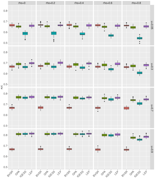
Figure 9: Performance of risk variants identification measured by AUC for the case-control studies

Fig. 9 indicate that LEP and GPA have comparable performances in terms of risk variants identification, they all outperform IGESS and BVSR.

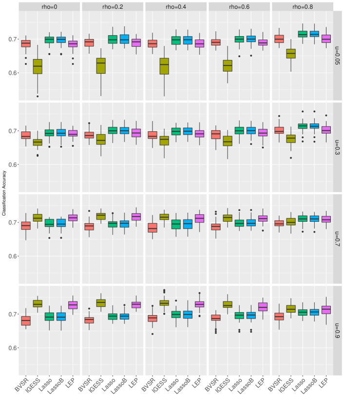
Figure 10: Performance of classification accuracy, which is measured by AUC evaluated on the observed phenotype values and the predicted values, Lasso corresponds to Lasso of Gaussian type, LassoB corresponds to Lasso of Binomial type. Lasso and LassoB have very similar performances.

Fig. 10 shows that LEP has comparable performance with BVSR where the summary-level data is irrelevant, LEP outperforms BVSR under all other settings which shows that the information from the summary-level data has been utilized effectively, and LEP outperforms Lasso and LassoB with low LD ($\rho=\{0,0.2,0.4,0.6\}$) and higher pleiotropy effects ($u=\{0.7,0.9\}.$)

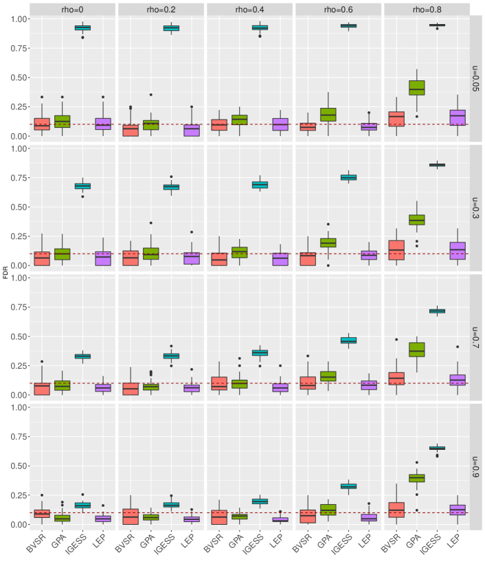
Figure 11: Performance of False Discovery Rate (FDR) Control at pre-specified level $FDR=0.1$ for the case-control studies

As the results shown Fig. 11, LEP could control FDR well with small or moderate LD as $\rho=\{0.2,0.4,0.6\}$, we have observed slightly inflated FDR when $\rho=0.8$ in the case-control studies.

5.5 The source of the five GWAS of Summary Statistics

We list the information in Table 2 for the summary statistics in the real data analysis, the information contains their associated sample size , their corresponding number of SNPs, their original paper and the link for downloading the datasets.

	N	M	Souce
Alzheimer	54,162	1,136,071	Lambert et al., 2013, Nature Genetics. https://data.broadinstitute.org/alkesgroup/sumstats_formatted/
Neuroticism	170,911	1,115,394	Okbay et al., 2016a, Nature Genetics. http://ssgac.org/documents/Neuroticism_Full.txt.gz
Type 1 Diabetes	26,890	915,518	Bradfield et al., 2011, PLoS Genetics. https://www.immunobase.org/downloads/protected_data/GWAS_Data
Ulcerative Colitis	27,432	1,076,835	Jostins et al., 2012, Nature. https://data.broadinstitute.org/alkesgroup/sumstats_formatted/
Primary Biliary Cirrhosis	13,239	525,775	Cordell et al., 2015, Nature Communications https://www.immunobase.org/downloads/protected_data/GWAS_Data/

Table 2: Basic information for the summary statistics for Alzheimer, Neuroticism, Type 1 diabetes, Ulcerative Colitis, Primary Biliary Colitis

Funding

This work was supported in part by grant NO. 61501389 and No. 11501440 from National Science Funding of China, grants NO. 12202114, NO. 22302815 and NO. 12316116 from the Hong Kong Research Grant Council, and Initiation Grant NO. IGN17SC02 from University Grants Committee, startup grant R9405 from The Hong Kong University of Science and Technology, ITF391/15FX (P0162) from innovative technology funding of Hong Kong, Duke-NUS Medical School WBS: R-913-200-098-263, MOE2016-T2-2-029 from Ministry of Eduction, Singapore and Shenzhen Fundamental Research Fund under Grant No. KQTD2015033114415450.

References

• Begovich et al. (2004) Begovich, A. B., Carlton, V. E., Honigberg, L. A., Schrodi, S. J., Chokkalingam, A. P., Alexander, H. C., Ardlie, K. G., Huang, Q., Smith, A. M., Spoerke, J. M., et al. (2004). A missense single-nucleotide polymorphism in a gene encoding a protein tyrosine phosphatase (PTPN22) is associated with rheumatoid arthritis. The American Journal of Human Genetics, 75(2), 330–337.
• Bishop (2006) Bishop, C. M. (2006). Pattern recognition and machine learning. Springer.
• Burton et al. (2007) Burton, P. R., Clayton, D. G., Cardon, L. R., Craddock, N., Deloukas, P., Duncanson, A., Kwiatkowski, D. P., McCarthy, M. I., Ouwehand, W. H., Samani, N. J., et al. (2007). Genome-wide association study of 14,000 cases of seven common diseases and 3,000 shared controls. Nature, 447(7145), 661–678.
• Carbonetto and Stephens (2012) Carbonetto, P. and Stephens, M. (2012). Scalable variational inference for bayesian variable selection in regression, and its accuracy in genetic association studies. Bayesian analysis, 7(1), 73–108.
• Chung et al. (2014) Chung, D., Yang, C., Li, C., Gelernter, J., and Zhao, H. (2014). GPA: a statistical approach to prioritizing GWAS results by integrating pleiotropy and annotation. PLoS genetics, 10(11), e1004787.
• Cotsapas et al. (2011) Cotsapas, C., Voight, B. F., Rossin, E., Lage, K., Neale, B. M., Wallace, C., Abecasis, G. R., Barrett, J. C., Behrens, T., Cho, J., et al. (2011). Pervasive sharing of genetic effects in autoimmune disease. PLoS genetics, 7(8), e1002254.
• Cross-Disorder Group of the Psychiatric Genomics Consortium (2013) Cross-Disorder Group of the Psychiatric Genomics Consortium (2013). Identification of risk loci with shared effects on five major psychiatric disorders: a genome-wide analysis. The Lancet, 381(9875), 1371–1379.
• Dai et al. (2017) Dai, M., Ming, J., Cai, M., Liu, J., Yang, C., Wan, X., and Xu, Z. (2017). IGESS: a statistical approach to integrating individual-level genotype data and summary statistics in genome-wide association studies. Bioinformatics, 33(18), 2882–2889.
• Efron (2010) Efron, B. (2010). Large-scale inference: empirical Bayes methods for estimation, testing, and prediction, volume 1. Cambridge University Press.
• Flannick and Florez (2016) Flannick, J. and Florez, J. C. (2016). Type 2 diabetes: genetic data sharing to advance complex disease research. Nature Reviews Genetics, 17(9), 535.
• Kang et al. (2010) Kang, H. M., Sul, J. H., Service, S. K., Zaitlen, N. A., Kong, S.-y., Freimer, N. B., Sabatti, C., Eskin, E., et al. (2010). Variance component model to account for sample structure in genome-wide association studies. Nature genetics, 42(4), 348–354.
• Khera and Kathiresan (2017) Khera, A. V. and Kathiresan, S. (2017). Genetics of coronary artery disease: discovery, biology and clinical translation. Nature Reviews Genetics, 18(6), 331.
• Li et al. (2014) Li, C., Yang, C., Gelernter, J., and Zhao, H. (2014). Improving genetic risk prediction by leveraging pleiotropy. Human genetics, 133(5), 639–650.
• Liu et al. (2016) Liu, J., Wan, X., Ma, S., and Yang, C. (2016). EPS: an empirical Bayes approach to integrating pleiotropy and tissue-specific information for prioritizing risk genes. Bioinformatics, 32(12), 1856–1864.
• Liu et al. (2017) Liu, J., Wan, X., Wang, C., Yang, C., Zhou, X., and Yang, C. (2017). LLR: a latent low-rank approach to colocalizing genetic risk variants in multiple GWAS. Bioinformatics, 33(24), 3878–3886.
• Mak et al. (2017) Mak, T. S. H., Porsch, R. M., Choi, S. W., Zhou, X., and Sham, P. C. (2017). Polygenic scores via penalized regression on summary statistics. Genetic epidemiology, 41(6), 469–480.
• Mitchell and Beauchamp (1988) Mitchell, T. J. and Beauchamp, J. J. (1988). Bayesian variable selection in linear regression. Journal of the American Statistical Association, 83(404), 1023–1032.
• Pasaniuc and Price (2017) Pasaniuc, B. and Price, A. L. (2017). Dissecting the genetics of complex traits using summary association statistics. Nature Reviews Genetics, 18(2), 117.
• Purcell et al. (2007) Purcell, S., Neale, B., Todd-Brown, K., Thomas, L., Ferreira, M. A., Bender, D., Maller, J., Sklar, P., De Bakker, P. I., Daly, M. J., et al. (2007). PLINK: a tool set for whole-genome association and population-based linkage analyses. The American Journal of Human Genetics, 81(3), 559–575.
• Purcell et al. (2009) Purcell, S. M., Wray, N. R., Stone, J. L., Visscher, P. M., O’donovan, M. C., Sullivan, P. F., Sklar, P., Ruderfer, D. M., McQuillin, A., Morris, D. W., et al. (2009). Common polygenic variation contributes to risk of schizophrenia and bipolar disorder. Nature, 460(7256), 748–752.
• Shi et al. (2016) Shi, J., Park, J.-H., Duan, J., Berndt, S. T., Moy, W., Yu, K., Song, L., Wheeler, W., Hua, X., Silverman, D., et al. (2016). Winner’s curse correction and variable thresholding improve performance of polygenic risk modeling based on genome-wide association study summary-level data. PLoS genetics, 12(12), e1006493.
• Sivakumaran et al. (2011) Sivakumaran, S., Agakov, F., Theodoratou, E., Prendergast, J. G., Zgaga, L., Manolio, T., Rudan, I., McKeigue, P., Wilson, J. F., and Campbell, H. (2011). Abundant pleiotropy in human complex diseases and traits. The American Journal of Human Genetics, 89(5), 607–618.
• Stearns (2010) Stearns, F. W. (2010). One hundred years of pleiotropy: a retrospective. Genetics, 186(3), 767–773.
• Tibshirani (1996) Tibshirani, R. (1996). Regression shrinkage and selection via the lasso. Journal of the Royal Statistical Society. Series B (Methodological), pages 267–288.
• Turley et al. (2018) Turley, P., Walters, R. K., Maghzian, O., Okbay, A., Lee, J. J., Fontana, M. A., Nguyen-Viet, T. A., Wedow, R., Zacher, M., Furlotte, N. A., et al. (2018). Multi-trait analysis of genome-wide association summary statistics using MTAG. Nature genetics, 50, 229–237.
• Visscher et al. (2017) Visscher, P. M., Wray, N. R., Zhang, Q., Sklar, P., McCarthy, M. I., Brown, M. A., and Yang, J. (2017). 10 years of gwas discovery: biology, function, and translation. The American Journal of Human Genetics, 101(1), 5–22.
• Welter et al. (2014) Welter, D., MacArthur, J., Morales, J., Burdett, T., Hall, P., Junkins, H., Klemm, A., Flicek, P., Manolio, T., Hindorff, L., et al. (2014). The NHGRI GWAS Catalog, a curated resource of SNP-trait associations. Nucleic Acids Research, 42(D1), D1001–D1006.
• Yang et al. (2015) Yang, C., Li, C., Wang, Q., Chung, D., and Zhao, H. (2015). Implications of pleiotropy: challenges and opportunities for mining big data in biomedicine. Frontiers in genetics, 6, 229.
• Yang et al. (2016) Yang, C., Wan, X., Liu, J., and Ng, M. (2016). Introduction to statistical methods for integrative data analysis in genome-wide association studies. In Big Data Analytics in Genomics, pages 3–23. Springer.
• Yang et al. (2011) Yang, J., Lee, S. H., Goddard, M. E., and Visscher, P. M. (2011). GCTA: a tool for genome-wide complex trait analysis. The American Journal of Human Genetics, 88(1), 76–82.
• Zhu et al. (2015) Zhu, X., Feng, T., Tayo, B. O., Liang, J., Young, J. H., Franceschini, N., Smith, J. A., Yanek, L. R., Sun, Y. V., Edwards, T. L., et al. (2015). Meta-analysis of correlated traits via summary statistics from GWASs with an application in hypertension. The American Journal of Human Genetics, 96(1), 21–36.