Wind and nebula of the M 33 variable GR 290 (WR/LBV)

Context: GR 290 (M 33/V532=Romano’s Star) is a suspected post-LBV (Luminous Blue Variable) star located in M 33 galaxy that shows a rare Wolf–Rayet (WR) spectrum during its minimum light phase. In spite of many studies, its atmospheric structure, its circumstellar environment and its place in the general context of massive stars evolution is poorly known.
Aims: Detailed study of its wind and mass loss, and study of the circumstellar environment associated to the star.
Methods: Long-slit spectra of GR 290 were obtained during its present minimum luminosity phase with the Gran Telescopio Canario covering the $\sim 3600-7500$ ÅÅ wavelength range together with contemporaneous BVRI photometry. The data were compared with non-local thermodynamical equilibrium (non-LTE) model atmosphere synthetic spectra computed with CMFGEN and with CLOUDY models for ionized interstellar medium regions.
Results: The current $m_{V}=18.8$ mag, is the faintest at which this source has ever been observed. The non-LTE models indicate effective temperature $T_{eff}=27000-30000$ K at radius $R_{2/3}=27-21$ ${\rm R_{\odot}}$ and mass loss rate $\dot{M}$=1.5$\times$10^-5 ${\rm M_{\odot}yr^{-1}}$. The terminal wind speed ${\mathrm{v}}_{\infty}$=620 ${\rm km\leavevmode\nobreak\ s^{-1}}$ is faster than ever before recorded while the current luminosity $L_{*}=(3.1-3.7)\times$10⁵ ${\rm L_{\odot}}$ is the lowest ever deduced. It is overabundant in He and N and underabundant in C and O. It is surrounded by an unresolved compact H II region with dimensions $\leq$4 pc, from where H-Balmer, He i lines and $[{O\textsc{III}}]$ and $[{N\textsc{II}}]$ are detected. In addition, we find emission from a more extended interstellar medium (ISM) region which appears to be asymmetric, with a larger extent to the East ($16-40$ pc) than to the West.
Conclusions: In the present long lasting visual minimum, GR 290 is in a lower bolometric luminosity state with higher mass loss rate. The nearby nebular emission seems to suggest that the star has undergone significant mass loss over the past $10^{4}-10^{5}$ years and is nearing the end stages of its evolution.

1 Introduction

Luminous Blue variables (LBVs) are relatively short evolutionary stage in life of massive stars. During this phase they lose significant mass through strong stellar winds and occasional giant eruptive events. As result, they shed their outer layers and eventually become hydrogen-deficient Wolf–Rayet (WR) stars (Langer et al. 1994; Humphreys & Davidson 1994; Ekström et al. 2012; Groh et al. 2013b).

LBVs show both short timescale stochastic variability with amplitude up to few tenths of mag (Humphreys & Davidson 1994; Abolmasov 2011) and long-term variability, so-called S Dor cycle (Humphreys & Davidson 1994; Vink 2012; Humphreys et al. 2016). Typically S Dor cycles last for several years and their amplitude is $1-3$ mags. During S Dor cycle photometric variability is always accompanied by changes in effective temperature, i.e. their spectral type changes in the range from B supergiants or late Of/WN stars to A-supergiants. At the same time, the bolometric luminosity remains approximately constant (Wolf 1989; Humphreys & Davidson 1994) or may even decrease during the visual maximum (Groh et al. 2009). Moreover, Galactic objects $\eta$ Car and P Cyg have shown another kind of outbursts, so-called giant eruptions – huge increase of bolometric luminosity simultaneously with an increase of visual brightness (Humphreys & Davidson 1994).

LBVs are divided into two subclasses: low luminosity LBVs and classical LBVs (Humphreys et al. 2016). The former ones originate from stars with $M_{*}\approx 25-40\,\rm M_{\odot}$ reaching LBV stage after being red supergiants (RSG) (Humphreys et al. 2016; Meynet & Maeder 2005). Groh et al. (2013a) demonstrated that low luminosity LBVs could be progenitors of Supernovae (SN) IIb. Thus low luminosity LBVs are final stage of stellar evolution, rather than a transitory evolutionary phase between RSG and WR as was suggested earlier (Meynet & Maeder 2005).

Classical LBVs originate from more massive stars ($M_{*}\approx 40-60\,\rm M_{\odot}$) moving off the Main Sequence (MS) and evolving towards the WR stage via blue supergiant (BSG) and LBV phases (Meynet & Maeder 2005; Meynet et al. 2011). According to Groh et al. (2014), stars with $60\,\rm M_{\odot}$ are spending $2\cdot 10^{5}$ years in LBVs phase, i.e., only 5% of their lifetime. Consideration of the initial mass function (IMF) leads to conclude that LBV stars are extremely rare and there should be no more than a few dozens such objects in the Galaxy. Clues to the mechanisms by which transition from O-type stars and WR stars occurs may be gleaned from a handful of objects that have been observed to display both WR and LBV characteristics. Examples of these rare objects include AG Car in our Galaxy (Groh et al. 2009), R 127 and HDE 269582 in Large Magellanic Cloud (Walborn et al. (2017) and references therein), HD 5980 in Small Magellanic Cloud (Koenigsberger et al. 2014) and GR 290 in M 33 (Polcaro et al. (2016), and references therein).

GR 290 (M 33-V532=Romano’s Star) is located in a relatively empty field in the outskirts of M 33 galaxy. It was first classified as a Hubble-Sandage variable by Romano (1978) and then became an LBV candidate (Humphreys & Davidson 1994; Szeifert 1996) after introduction of this class of objects by Peter Conti (1984). Spectral variations from a B-supergiant type spectrum to that of a WR of the nitrogen sequence (WN), photometric variability (Kurtev et al. 2001) as well as a large bolometric luminosity (Polcaro et al. 2003) are the reasons that led to the promotion of GR 290 from a LBV candidate to bona fide LBV (see Kurtev et al. (2001); Polcaro et al. (2003) and Fabrika et al. (2005)). Later, Polcaro et al. (2011) concluded that GR 290’s bolometric luminosity has significantly changed during the minimum phase of the 2008 year and suggested that Romano’s star has already passed through the LBV phase, i.e. that it is a post-LBV. Humphreys et al. (2014) noted that the star does not exhibit S Dor transitions to the cool, dense wind state – instead, it varies between two hot states on the Hertzsprung–Russell diagram, characterized by WN spectroscopic features (Humphreys et al. 2014). Humphreys et al. (2014) also, like Polcaro et al. (2011) earlier, suggested that Romano’s star is likely in a post-LBV state.

The photometric investigation initiated by Romano (1978) was followed by that of Kurtev et al. (2001), who reported the photometry obtained over 1982-1990. They concluded that the eruption time-scales are $\sim$20 years and that shorter timescale oscillations of $\sim$270 days or $\sim$320 days with amplitude of 0.5 mag are also present. Zharova et al. (2011) investigated photometric variability of GR 290 using both the Moscow collection of photographic plates, their own data, and the data published earlier (Romano 1978; Humphreys & Sandage 1980; Sholukhova et al. 2002; Viotti et al. 2006), thus constructing the most comprehensive light curve covering half a century. This light curve shows that GR 290 exhibits irregular brightness variations with different amplitudes and time scales, and where the large amplitude and complex wave-like variations on the scale of several years are the most prominent. Polcaro et al. (2016) were able to further extend this light curve to the beginning of 20th century and demonstrated that GR 290 did not display any significant eruptions between 1901 and the 1960s.

Studies of GR 290 devoted to spectral variability show that its spectral type changes between WN11 and WN8 (Maryeva & Abolmasov 2010; Polcaro et al. 2011; Sholukhova et al. 2011). Since the beginning of 2000s it has made this transition twice (Polcaro et al. 2016). Viotti et al. (2006, 2007) first described an anticorrelation between emission line strength and brightness. Then Maryeva & Abolmasov (2010) found a correlation of spectral changes and the visual brightness typical for LBVs: the brighter it is, the cooler the spectral type. However, among all known LBVs only HD 5980 convincingly shows a hotter spectrum in the minimum of brightness.

The models of GR 290 atmosphere have been constructed for three states – luminosity maximum of 2005 and the minimum of brightness in 2008 (Maryeva & Abolmasov 2012), and at the moderate luminosity maximum of 2010 (Clark et al. 2012). Polcaro et al. (2016) built nine models for the most representative spectra acquired between 2002 and 2014 and demonstrated how the GR 290 wind structure varies correlated with brightness changes – the slow and dense wind at brightness maxima becomes faster and thinner at minima. Similar correlations appear also in HD 5980 (Georgiev et al. 2011) and provide clues to the mechanisms that drive the spectral transitions. However, due to its faintness in recent years, it has been challenging to obtain the spectra of GR 290 with high enough quality for wind speeds to be adequately estimated.

Many LBVs are surrounded by small nebulae whose structure and chemical composition have been studied in order to investigate their past history (e.g. Martayan et al. (2016) and references therein). In this regard, Fabrika et al. (2005) claimed a marginal detection, in an H$\beta$ image, of a compact elongated nebula around GR 290. But no detailed spectrophotometric study of the nebular emission near GR 290 has been so far carried out.

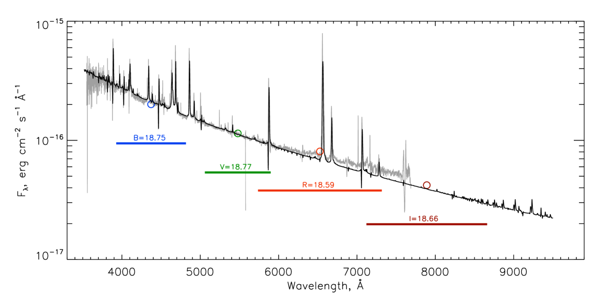
Figure 1: Flux-calibrated spectrum of GR 290 (grey line) compared with the best-fit $\beta$=2 CMFGEN model (black line). Measured photometric magnitudes and corresponding bandwidths are indicated. The model spectrum is scaled for the distance to the M 33 and the interstellar extinction ($E_{(B-V)}=0.06$) is applied to it. The adopted distance to M 33 is 847$\pm$61 kpc (distance module 24.64 $\pm$0.15) from Galleti et al. (2004).

In this paper we present the results of our ongoing spectral and photometric monitoring of GR 290. We report the results of observations performed in 2016 with one of the best spectral resolutions and signal-to-noise ratio ever obtained for this object. We are particularly targeting the information on the circumstellar emission around GR 290 that may be extracted from these spectra, which may give us some knowledge on the mass loss during previous stages of the star’s life.

In section 2 we describe the observations; in section 3 the current spectral characteristics and deduced parameters from CMFGEN fits; in section 4 the spectral characteristics of the interstellar medium and OB-star regions in the neighborhood of GR 290. In section 5 we present the conclusions.

2 Observations

GR 290 was observed with the OSIRIS spectrograph on the Gran Telescopio Canarias (GTC) on 2016 July 30 and August 27 (MJD 57599.1569, 57627.073, respectively) in Service Observing mode using the R2500-set of gratings and the long slit (7.4’) with a slit width of 0.6”. These gratings cover the ultraviolet ($U$), visual ($V$) and red ($R$) wavelength intervals as defined in the third column of Table 1. This table also lists the filter ID, the exposure time, the range in signal-to-noise (S/N), the spectral dispersion and the resolution for each of the observations. Position angles were $94.75\deg$ and $95.2\deg$, respectively.

Table 1: Spectroscopic observations 2016 July and August.

MJD	Filter ID	$\lambda$-range	$t_{exp}$	S/N	Å/pix	Res.
		(Å)	(s)
57599.16	R2500U	3440 - 4610	1200	40-50	0.62	2555
57627.07	”	”	1200	20-40	”	”
57599.17	R2500V	4500 - 6000	900	25-46	0.80	2515
57627.09	”	”	900	25-50	”	”
57599.18	R2500R	5575 - 7685	600	30-37	1.04	2475
57627.10	”	”	600	20-27	”	”

The spectra were pre-processed by the standard GTC/OSIRIS pipeline (Ederoclite & Cepa 2010). The data were then reduced using the standard IRAF procedures , which included the bias and flat field corrections as well as the wavelength calibration. The rms of the fit for the wavelength calibration on the comparison lamps is 0.032 Å in the red and 0.015 Å in visual and blue spectra. Lines lying on overlapping segments obtained from the 3 filters were checked for relative shifts. These lines are He i 4471 Å which appears in both the $U$ and the $V$ segments and the He i 5876 Å which appears in the $V$ and $R$ segments. Both lines have P Cyg profiles and we measured the emission and the absorption components separately as individual features, for the purpose of verifying the wavelength calibration. We find that the $U$ and $V$ segments overlap to within $\pm$0.2 Å at $\lambda$4471 in both the July and August observations. The $V$ and $R$ segments overlap to within $\pm$0.3 Å in the August observation. However, He i 5876 Å line in the $R$ segment in the July observation is shifted by about $-1$ Å  the source of which we are unable to ascertain. Although such a significant shift is not present in other lines of this R segment, we deem the RVs from this segment to be less reliable than those in the others.

The flux calibration was performed using standard routines in IRAF, as well as IDL procedures originally written for SCORPIO data reduction. The resulting flux-calibrated spectra, however, still suffer from the following limitations: 1) the lack of an accurate and updated extinction curve of the site, mainly in the red and 2) the fact that the standard star that was used is more than 10 magnitudes brighter than GR 290 so that the instrument was de-focused in order to avoid saturation. The absolute fluxes (shown in Fig. 1) are thus to be considered only approximate.

Table 2: Photometry obtained on 2016 Jul 31 using the Johnson-Cousins filters.

Band	magnitude	$\pm$	S/N	UT
V	18.77	0.04	71	01:44:14
R	18.59	0.04	72	01:53:10
I	18.66	0.05	46	02:00:57
B	18.75	0.03	99	02:10:43

Photometric observations in the Johnson-Cousins filters were obtained using the 1.52-m Cassini Telescope run by INAF-Osservatorio Astronomico di Bologna in Loiano on 2016 July 31, providing a photometric reference for the GTC July 30 observation. Table 2 lists in column 1 the wavelength band, in column 2 the magnitude value, in column 3 and 4 the measurement uncertainty and the S/N, respectively, and in column 5 the Universal Time (UT) of the observations. With $m_{V}=18.8\,{\rm mag}$, GR 290 is currently at its faintest since the beginning of the 20th century (see Polcaro et al. (2016) for the photometric history).

Table 3: Emission line radial velocity, FWHM and equivalent width measurements.

		—- July —-		—- August —		———– Average ————-
ID		RV	FWHM	RV	FWHM	RVem	-EW	Vabs	$V_{edge}$
He I	3704.00?	-15.	332.	-56.	307.	135	1.1	-210	-250
H I	3750.20	-129.	328.	…	…	16	0.6	-172	-283:
H I	3770.60	-102.	358.	-85.	374.	75	1.8	-258	-400:
H I	3797.90	-105.	308.	…	…	-10	0.4	-221	-310
He I	3819.60*	-178.	361.	-136.	228.	17	1.2	-252	-530
H I	3835.40*	-147.	320.	-104.	461.	32	1.2	-201	-370:
He I	3888.65	-149	457	-183	485:	20	10.4	-350	-660
H I	3970.10*	-124.	325.	-149.	310.	18	2.2	-193	…
He I	4026.20*	-149.	342.	-152.	342.	10	2.4	-248	-550
N IV	4057.76	-223.	273.	-164.	148.	-10	0.5	…	…
Si IV	4088.70*	-182.	213.	-173.	198.	2	1.7	…	…
N III	4097.30	-200.	154.	-190.	…	-4	2.0:	-230	-438
H I	4101.74	-67.	373.	-51.	285.	121:	5.2	…	…
Si IV	4116.10*	-228.	364.	-211.	233.	-32	2.8	…	…
N III	4195.76	-234.	141.	-266.	164.	-66:	0.2	…	…
N III	4200.10	-162.	206.	-165.	142.	13	0.6	-159:	-260:
H I	4340.50*	-149.	380.	-119.	366.	42	7.9	…	…
N III	4379.20*	-186.	260.	-164.	226.	-7	1.0	…	…
He I	4387.90*	-198.	301.	-135.	246.	13	1.6	…	…
He I	4471.50*	-149.	389.	-127.	362.	28	4.9	-275	-630
N III	4534.60*	-194.	178.	-149.	165.	-22	0.4:	-233:	-280:
He II	4541.60	-145.	145.	…	…	29:	2.0:	-182	-300:
N III	4634.14	-183	256	-188	252	-9	5.5	…	…
N III	4640.64	-197.	252.	-195.	258.	-16	9.4	…	…
He II	4685.6 *	-176.	333.	-174.	326.	7	17.4	…	…
He I	4713.1 *	-146.	197.	-130.	407.	28	1.6:	-291	-500:
H I	4861.3 *	-171.	395.	-167.	401.	11	18.2	…	…
He I	4921.9 *	-185.	335.	-174.	371.	4	4.3	…	…
He I	5015.7 *	-162.	275.	-149.	287.	15	1.7	-200:	…
He I	5047.7 *	-174.	184.	-143.	237.	41	0.6	…	…
He II	5411.52	-150.	260.	-169.	294.	15	1.9	-217	-433
He I	5875.66*	-175.	444.	-171.	464.	5	24.5	-304	-655
H I	6562.80	-184.	301.	-176.	269.	-1	…	…	…
H I	6562.80*	-181.	466.	-172.	461.	8	68.0	…	…
He I	6678.15*	-176.	417.	-185.	395.	-6	18.0	…	…
He I	7065.20*	-152.	467.	-157.	450.	13	18.1	-306	-560
N IV	7109.35	-169.	181.	…	…	8	0.2:	…	…
N IV	7122.98	-160.	231.	…	…	…	0.3	…	…

Notes: Columns: 1 lists the primary atomic identification and corresponding laboratory wavelength in Å; 2 and 4 list the RVs for, respective, the July and the August observations after applying the heliocentric corrections of $+27\leavevmode\nobreak\ {\rm km\leavevmode\nobreak\ s^{-1}}$ for July and $+24\leavevmode\nobreak\ {\rm km\leavevmode\nobreak\ s^{-1}}$ for of August; 3 and 5 are the corresponding full-widths at half maximum intensity. Columns 6-9 list measurements performed on the combined July+August spectrum after correcting for the adopted -179 ${\rm km\leavevmode\nobreak\ s^{-1}}$ systemic velocity of M 33. Column 6 is the RV of the emission lines; column 7 is the corresponding equivalent width; column 8 is the centroid of the P Cyg absorption component when present; and column 9 is the velocity of the P Cyg absorption edge (i.e., the location where the absorption reaches the continuum). RVs and FWHM’s are in units of ${\rm km\leavevmode\nobreak\ s^{-1}}$; EWs are in units of Å, and the negative sign in the column heading indicates emission. Asterisk indicates the line was used to determine the RV of the system.

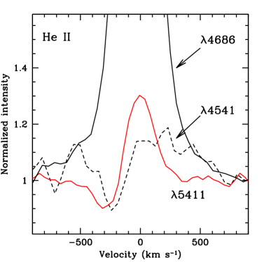
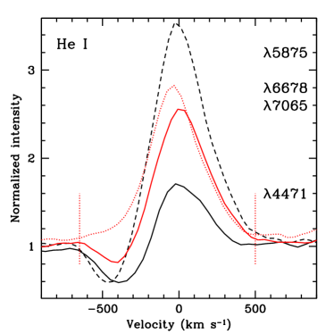
Figure 2: Left: Line profiles of He ii plotted on a velocity scale corrected for the adopted -179 ${\rm km\leavevmode\nobreak\ s^{-1}}$ systemic velocity. The continuous line shows the strong $\lambda$4686, with its extended electron scattering wings and $\lambda$5411 with its strong P Cyg absorption. The dash line is $\lambda$4541 which is contaminated on the blue wing with N III. Right: He i lines profiles of $\lambda$4471 (continuous, black), $\lambda$5876 (dash, black), $\lambda$6678 (dot, red) and $\lambda$7065 (continuous, red). The vertical lines indicate the approximate locations where the line meets the continuum level.

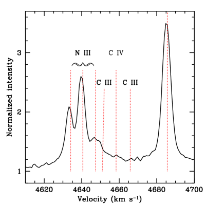
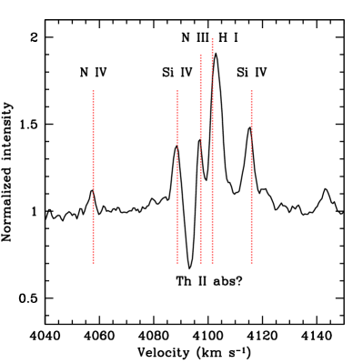
Figure 3: Line profiles on a wavelength scale corrected for the adopted -179 ${\rm km\leavevmode\nobreak\ s^{-1}}$ systemic velocity of M 33. Left: N III 4634-41 and He ii 4686 emission lines. Note the possible contribution of C IV. Right: N IV 4058 and the 4100 Å blend that includes Si IV, N III and H I lines. Vertical lines indicate the laboratory wavelength of the transitions.

3 Spectrum of GR 290

The flux calibrated spectrum of GR 290 is characterized by a blueward rising continuum and strong emission lines, as illustrated in Fig. 1. In addition to H$\alpha$ and H$\beta$, the spectrum is dominated by lines from He i, He ii and N III. The P Cyg absorption components of the He i triplet lines are enhanced, with respect to the singlets, due to the overpopulation with respect to LTE of the low-lying triplet levels in the low density stellar wind. The He II Paschen-like line at 4686 Å (3-4) is observed in emission, as in earlier spectra, while the multiplet 2 Brackett-like lines at 5411 Å (4-7) and 4541 Å (4-9) have P Cyg profiles and are now stronger than in earlier spectra. The He ii line from this same series at 4199 Å (4-11) (blended with N III) also displays a P Cyg profile. The profiles of some of the He ii lines are illustrated in Fig. 2.

The strongest N III lines are those at 4634-41 Å, which are partially resolved (Fig. 3, left). There is a prominent absorption blueward of N III 4097 Å suggesting that this line also has a P Cyg profile. The N III 4196, 4200 and 4379 Å are also now present, consistent with a higherd egree of ionization in the wind suggested by the increased strength of He ii 5411.

Most importantly, we note the presence for the first time of N IV 4058 Å in Fig. 3 (right). It is clearly present in both the July and the August spectra and has an equivalent width of 0.5 Å on the combined spectrum. The N IV lines at 7109 and 7122 Å appear to also be weakly present.

The primary indicator of ionization classification given by Smith et al. (1996) is the ratio of equivalent widths (EW) of He II 5411/He I 5876 Å. We find that this ratio is $\leq$0.1, implying a degree of ionization corresponding to WN8. The earlier criteria of van der Hucht et al. (1981),which are based on the Smith (1968) system, rely on the ratios of N III/N IV/N V 4634-4641, 4057 and 4604-4620 Å, respectively. The fact that EW(N III) $\gg$ EW(N IV) is consistent with WN8 or cooler (see Table 3).

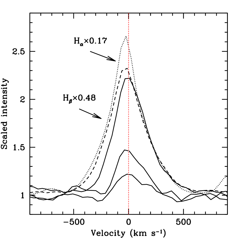
Figure 4: Line profiles of the Balmer-H sequence plotted on a velocity scale corrected for the adopted -179 ${\rm km\leavevmode\nobreak\ s^{-1}}$ systemic velocity. The lines of H$\alpha$ and H$\beta$ are scaled by factors of 0.17 and 0.48, respectively, so as to align the red wings with that of H$\gamma$. The continuous lines show H$\gamma$, H$\epsilon$ and H I 3835 Å. The progressive red-shift at shorter wavelengths appears to be a consequence of the increasing strength of the blue-shifted absorption which, in the helium lines, takes on the form of P Cyg absorption. This effect is explained by the fact that the optical depth of the wind is highest for H$\alpha$ and H$\beta$ and decreases for lines having smaller transition probabilities.

3.1 Radial Velocities

The radial velocity (RV) and full-width at half maximum intensity (FWHM) was obtained through a Gaussian fit to individual line profiles or, in the case of overlapping lines and P Cyg profiles, through simultaneous multiple Gaussian fits. Table 3 contains the results of our measurements. Columns 1 and 2 list the primary atomic identification and corresponding laboratory wavelength, Columns 3 and 5 list the heliocentric RV of the line centroid for, respective, the July and the August observations. The corresponding heliocentric corrections are $+27\leavevmode\nobreak\ {\rm km\leavevmode\nobreak\ s^{-1}}$ for July and $+24\leavevmode\nobreak\ {\rm km\leavevmode\nobreak\ s^{-1}}$ for August. Columns 4 and 6 list the corresponding values of the FWHM.

In order to obtain the velocity of GR 290 with respect to M 33, we averaged the RVs of the lines in Table 3 marked with an asterisk. The selection of these lines is based on the following criteria: 1) relatively unblended line; 2) relatively good S/N; 3) little or no ambiguity in the identification. We find average RV(July)=-171$\pm$22 (s.d.) ${\rm km\leavevmode\nobreak\ s^{-1}}$ and RV(August)=-155$\pm$24 (s.d.) ${\rm km\leavevmode\nobreak\ s^{-1}}$. Averaging the RVs of July and August yields RV(GR 290)=-163$\pm$32 ${\rm km\leavevmode\nobreak\ s^{-1}}$. The three averages are consistent, within the uncertainties, with each other and with the heliocentric velocity -179$\pm$3 ${\rm km\leavevmode\nobreak\ s^{-1}}$ of M 33 . We thus adopt this latter value for the systemic velocity of GR 290 in the remainder of this paper. The standard deviations are of similar value to our estimated measurement uncertainty of $\pm$30 ${\rm km\leavevmode\nobreak\ s^{-1}}$.

Since we do not detect variability in our two spectra that is larger than the uncertainty discussed above, we combined the July and August spectra, shifted the average by +179 ${\rm km\leavevmode\nobreak\ s^{-1}}$ and remeasured the lines. We list in Table 3 the RV of the emission in Column 7, the equivalent width in Column 8, the RV of the absorption component in the case of P Cyg profiles in Column 9, and the intersection of the P Cyg absorption with the continuum level in Column 10. The measurements for P Cyg profiles were performed with two-Gaussian fits. We note that the contribution of nebular emission affects the FWHM. For example, in the case of $H\alpha$, we measure FWHM=6.6 Å if the line is fit with a single Gaussian while FWHM=10.2 Å if the line is treated as a blend of a broad stellar line and a narrow superposed nebular emission. Despite this large difference in FWHM, the RV in both cases is nearly the same.

The average $V_{edge}$=-400$\pm$144 ${\rm km\leavevmode\nobreak\ s^{-1}}$, is similar to the value of ${\mathrm{v}}_{\infty}$ listed in Polcaro et al. (2016) for recents spectra. However, the He I lines have $V_{edge}\simeq$620 ${\rm km\leavevmode\nobreak\ s^{-1}}$, implying wind speeds that are faster than ever before observed.

The Balmer-H lines also show the signs of a relatively fast outflow, as can be seen from the growing asymmetry in the blue wing of the higher excitation lines of this series. This is illustrated in Fig. 4 where H$\alpha$ and H$\beta$ were scaled in intensity so as to align the red wings with that of H$\gamma$. The other lines plotted are H$\epsilon$ and H i 3835 Å. This asymmetry results from the same process that leads to P Cyg absorptions in He i but because of the large optical depth of the H-lines, a fully developed absorption component is not visible.

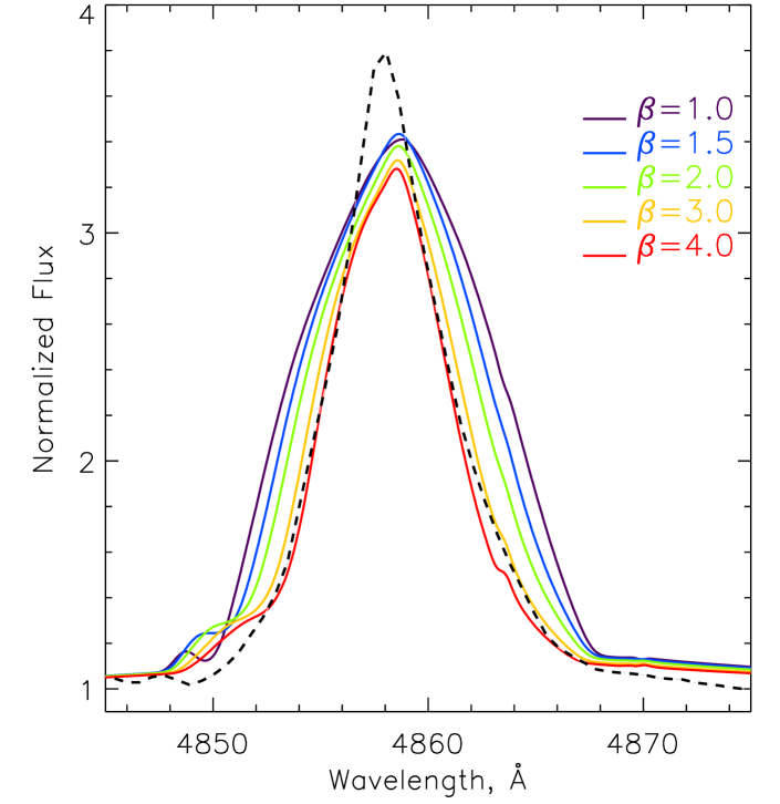
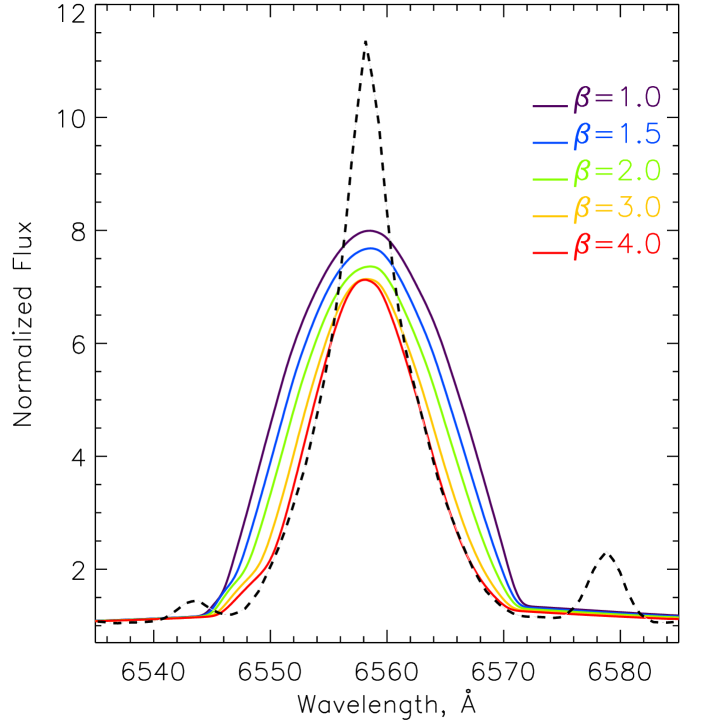
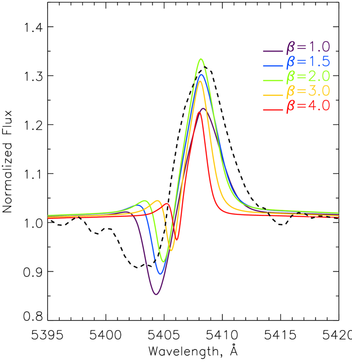
Figure 5: The effect of increasing $\beta$-parameter in the velocity law on spectral line profiles. From left to right – modeled profiles of H$\beta$, H$\alpha$ and He II 5411. For comparison, the actual profiles observed in the spectrum of GR 290 are shown by black dashed line.

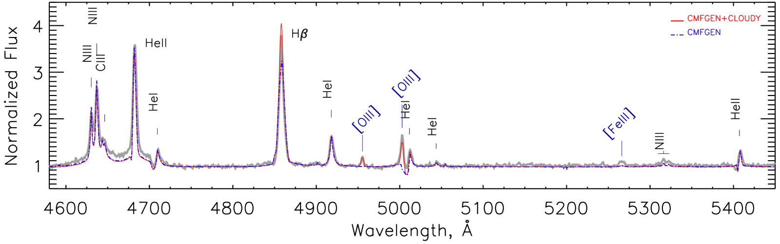
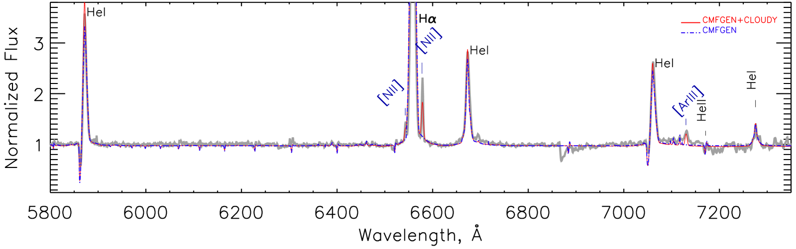
Figure 6: Normalized optical spectrum of GR 290 (grey line) compared with the best-fit CMFGEN model with $\beta=2$ (blue dash-dotted line). Red solid line shows the sum of CMFGEN (stellar atmosphere) and CLOUDY (surrounding nebula) models. The CLOUDY model has increased value of oxygen abundance (in comparison with the CMFGEN model), which we discuss in the text.

Table 4: Chemical abundances in the CMFGEN model.

Species	Rel. Num. Frac.	Mass Frac	NH	$Z/Z_{\odot}$
H	2.2	0.35	12	0.5
He	1.0	0.64	11.66	2.3
C	$1\times 10^{-4}$	$2\times 10^{-4}$	7.66	0.06
N	$1.5\times 10^{-3}$	$3.5\times 10^{-3}$	8.83	3.0
O	$1\times 10^{-4}$	$2.5\times 10^{-4}$	7.66	0.03
Ne	$2.4\times 10^{-4}$	$7.8\times 10^{-4}$	8.04	0.45
Mg	$5.0\times 10^{-5}$	$2.0\times 10^{-4}$	7.37	0.3
Al	$8.4\times 10^{-6}$	$3.7\times 10^{-5}$	6.58	0.65
Si	$3.0\times 10^{-5}$	$1.4\times 10^{-4}$	7.14	0.2
S	$2.3\times 10^{-5}$	$1.2\times 10^{-4}$	7.02	0.32
Ar	$6.5\times 10^{-6}$	$4.2\times 10^{-5}$	6.47	0.4
Ca	$4.2\times 10^{-6}$	$2.7\times 10^{-5}$	6.28	0.4
Fe	$4.9\times 10^{-5}$	$4.4\times 10^{-4}$	7.4	0.32

3.2 Stellar wind models

We used the CMFGEN atmospheric modeling code (Hillier & Miller 1998) in order to estimate the current stellar parameters of GR 290. This code solves the radiative transfer equation for objects with spherically symmetric extended outflows using either the Sobolev approximation or the full comoving-frame solution of the radiative transfer equation. CMFGEN incorporates line blanketing, the effect of Auger ionization and clumping, which is parametrized by the volume filling factor $f=\bar{\rho}/\rho(r)$, where $\bar{\rho}$ is the homogeneous (unclumped) wind density and ${\rho}$ is the density inside clumps assumed to be optically thin to radiation, while the interclump medium is void (Hillier & Miller 1999). Every model is defined by a hydrostatic stellar radius $R_{*}$, luminosity $L_{*}$, mass-loss rate $\dot{M}$, filling factor $f$,wind terminal velocity ${\mathrm{v}}_{\infty}$, stellar mass $M$ and by the abundances $Z_{i}$ of the chemical elements that are included. LBVs may have inflated radii and pseudophotospheres (Gräfener et al. 2012), which may cause large uncertainties in the the $R_{*}$ value derived from CMFGEN. Thus, hydrodynamical models need to be used to compute the hydrostatic radius and when discussing the evolutionary status of these objects, which goes beyond the scope of our current investigation.

The CMFGEN models were computed in an iterative manner, starting from an initial model and then adjusting parameters until a reasonable match between the model and observed spectra was attained. The temperature $T_{\rm{eff}}$ was first adjusted by using the ratios of He II/He I and N II/N III/N IV. Then the luminosity was adjusted by comparing with the contemporary $V$-band and $B-V$ photometry (see Table 2). The value of $\dot{M}$ was obtained from the line intensities, and the ${\mathrm{v}}_{\infty}$ from the P Cyg profile shapes. The filling factor $f$=0.15 was determined by fitting emission line profiles.

The abundances of chemical elements used in the models are listed in Table 4. The relative number fraction is given in column 2, the corresponding mass fraction in column 3,the adopted solar abundance in column 4 and the model abundance relative to the solar abundance in column 5. The abundances of H, He, C, N, and O were estimated from the model, while for the abundances of Ar, S and Ne we used those of M 33 from Magrini et al. (2010). For the abundances of other elements (Mg, Al, Si, Ca and Fe) we assumed a values of half solar as the metallicity of the outer regions of M 33 is low.

Beta velocity law ${\mathrm{v}}(r)={\mathrm{v}}_{\infty}\left(1-\frac{R_{*}}{r}\right)^{\beta}$ approximation is one of the basic simplifications typically adopted while constructing atmospheric models of hot stars. Radiation-driven wind theory (Puls et al. 1996; Lamers & Cassinelli 1999) predicts the values of $\beta=$ 0.5-1, while more hydrodynamically consistent numerical models favor $\beta=2.4$ for inner parts of the wind, and $\beta=0.9$ – for the outer ones (Sander et al. 2017). In our previous paper by Polcaro et al. (2016) we built the models assuming $\beta=1$, as our main goal was to compare the spectra acquired with different spectral resolutions and covering different spectral ranges in order to track the evolution of temperature, luminosity and mass loss rate over time. In the present article we are studying the spectrum with much better resolution covering the whole visible range, and immediately after starting the modeling process we have found that the profiles of hydrogen emission lines are not consistent with $\beta=1$. Therefore we had to build the models for several $\beta$ values. Fig. 5 illustrates the changes of lines’ profile with increasing $\beta$.

Table 5: CMFGEN model fit results.

Quantity	Model 1	Model 2	Note
${\rm L_{*}/10^{5}\times\,L_{\odot}}$	$(3.7\pm 0.2)$	$(3.1\pm 0.2)$
${\rm log(L_{*}/L_{\odot})}$	$5.57\pm 0.03$	$5.49\pm 0.03$
${\rm\dot{M}/10^{-5}\times\,M_{\odot}\leavevmode\nobreak\ yr^{-1}}$	$(1.5\pm 0.2)$	$(1.4\pm 0.2)$
${\rm R_{*}/R_{\odot}}$	$15-16.5$	$13.5-15.2$	(a)
${\rm T_{*}/K}$	$36000\pm 500$	$36000\pm 500$	(a)
${\rm R_{2/3}/R_{\odot}}$	$21-24.2$	$22.6-26.6$	(b)
${\rm T_{\rm eff}/K}$	$30000\pm 700$	$27500\pm 700$	(b)
${\rm{\mathrm{v}}_{\infty}/km\,s^{-1}}$	$620\pm 50$	$620\pm 50$
${\rm\beta}$	$2.0$	$3.0$

Notes: (a) The radius and temperature at the bottom of the wind where $\tau=18.7$; (b) The temperature and radius at $\tau=2/3$.

The models with $\beta=2$ and $\beta=3$ are closest to reproducing the observed spectrum. Both models provide a satisfactory fit to the overall spectral energy distribution and results of multicolor photometry as seen in Fig. 1, where the apparent discrepancy to the right of $\sim$6300 Å is caused by the uncertainties in the flux calibration and the adopted reddening correction, as well as the strong emission line here. The detailed comparison of observed spectrum with the best model with $\beta=2$ is shown in Fig. 6. The Fig. 7 clearly demonstrates that some lines are better described with $\beta=2$, while others – with $\beta=3$.

The models coincide relatively well with the broad portion of the H$\alpha$, H$\beta$ profiles, lying below the observed line maximum. This is consistent with the fact that GR 290 lies within a nebular region from which significant H-Balmer emission arises and which is responsible for the sharp superposed emission in these lines (see Sect. 4 below). The emission component of the He i P Cyg lines is well-reproduced by the models, but not so the absorption component which tends to be weaker than predicted. None of the models reproduces the profile shape of the high-excitation He II 5411 Å line, and this constitutes the largest discrepancy between the models and the observation. The model emission-line profile is a factor of $\sim$2 narrower and the absorption component is significantly less extended than the observations. Because of its high excitation, this line generally originates close to the hydrostatic photosphere where the wind is still accelerating. This discrepancy suggests that the emission-line forming region in GR 290 may be more complex than assumed in the model. That is, it may not be spherically symmetrical, or portions of the wind emission may be dominated by shock emission, factors which are not incorporated in the current CMFGEN model.

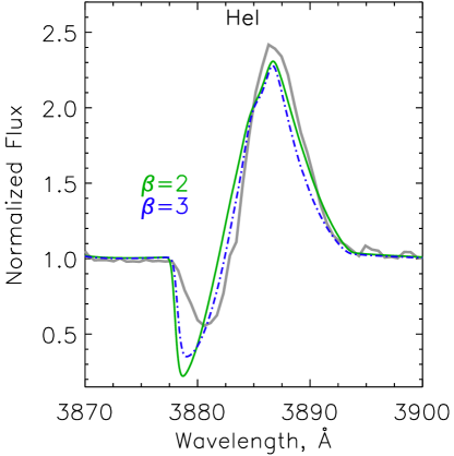
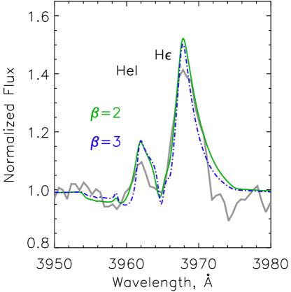
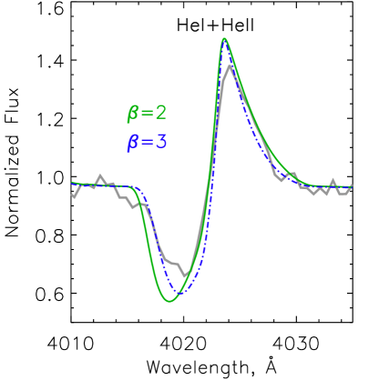
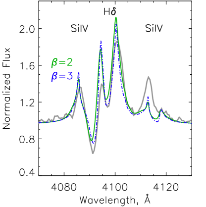
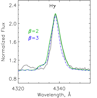
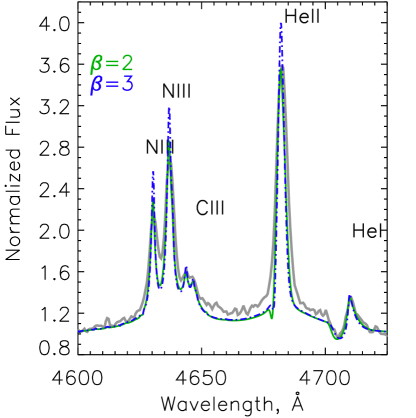
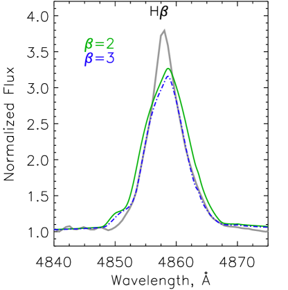
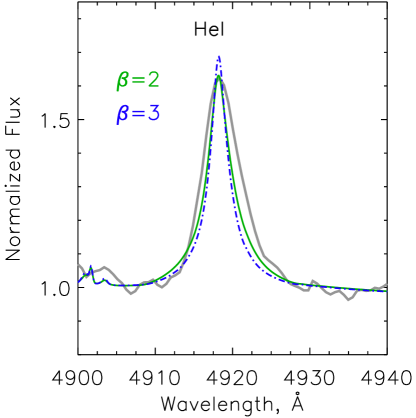
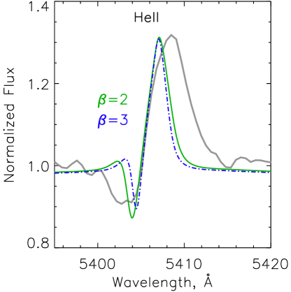
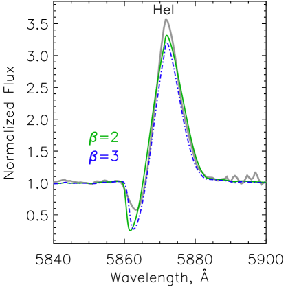
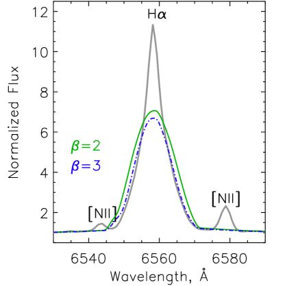
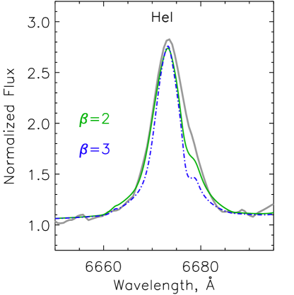
Figure 7: Comparison of the profiles of selected lines with the best model spectra.

4 The nebula surrounding GR 290

Circumstellar gaseous nebulae are formed around massive stars during BSG (Lamers et al. 2001) and LBV stages (Weis 2012). The sizes of these nebulae significantly increase under effect of fast stellar wind when the central stars transit to WR stage. Nebulae can tell us the history of its stars’ formation, ages, masses of ejected material. The presence of forbidden lines in the spectra of GR 290 indicates that it has a nebula, but the large distance prevents its detection on direct images. Below we investigate the structure of GR 290’s nebula using its two-dimensional spectrum.

The two-dimensional spectral image obtained with GTC contains information on the interstellar medium in the neighborhood of GR 290. The long OSIRIS slit was oriented in the East-West direction and in addition to GR 290, crosses the nearby OB88 and OB89 associations (Humphreys & Sandage 1980; Ivanov et al. 1993; Massey et al. 1995). OB89 and OB88 lie west of GR 290.

Figure 8 illustrates the tracing in the spatial dimension along the H$\alpha$ emission line. GR290 is at the origin of coordinates and appears sharp and narrow, compared to the other features in this tracing. From an analogous tracing at [N ii] 6548 Å  the spatial resolution is estimated to be $\sim$4 pixels, which is approximately 4 pc assuming a M 33 distance of 847 kpc. This is consistent with the limit imposed by the “seeing” of the observations: $\sim$1.2” in July and $\sim$1.6” in August.

A Gaussian fit to the sharp stellar emission peak indicates that there is considerable H$\alpha$ emission excess outside the wings of this fit, which can be associated with interstellar (ISM) emission. Specifically, the H$\alpha$ emission appears to extend for 9 pixels on the eastern side of the star but only for $\sim$4 pixels on the western side.

Table 6: Heliocentric radial velocities of nebular lines ($\rm{km\leavevmode\nobreak\ s^{-1}}$) August spectrum.

Position:	1	2	3
Line	GR 290	M 33-back	OB89
$[{S\textsc{II}}]\ 6716.44$	…	-208	-223
$[{S\textsc{II}}]\ 6730.82$	…	…	-226
$[{N\textsc{II}}]\ 6548.01$	-188	-147:	-180:a
$[{N\textsc{II}}]\ 6583.45$	-189	-233	-211
$H\alpha\ 6562.83$	-179	-194	-200
$[{O\textsc{III}}]\ 4958.90$	-206	…	…
$[{O\textsc{III}}]\ 5006.84$	-201b	…	…

Notes: ^a The [N ii]6548 Å line is significantly weaker than [N ii]6583 and is partially blended with the $H\alpha$ emission line. For this reason, we consider this measurement to have a larger uncertainty in RV than the rest, which is indicated with a colon (:) in the table; ^b [O iii]5007 was measured on the one-dimensional spectrum with a three-Gaussian fit to correct for the presence of the neighboring He i5015 Å line whose P Cyg absorption component overlaps its red wing.

The RVs of the more prominent ISM lines in the two-dimensional image are listed in Table 6. The measurements were performed at three locations along the spatial resolution axis. Position 1: centered on GR 290; Position 2: on the background close to GR 290, which provides information on the diffuse component of M 33 in the neighborhood of GR 290; and Position 3: centered on the OB89 cluster. Column 1 lists the principal emission line identification with its corresponding laboratory wavelength (Å); and columns 2-4 list the heliocentric RVs of the lines at Positions 1, 2 and 3, respectively. The averages ($\pm$ s.d.) of the lines at the three positions are, respectively -195 $\pm$14, -196$\pm$36 and -208$\pm$19 ${\rm km\leavevmode\nobreak\ s^{-1}}$, all consistent within the uncertainties with each other and with the systemic speed of M 33. The [N ii]6548 is quite extended and weak in the M 33-background surrounding GR 290 rendering its RV more uncertain than the rest. If we eliminate this line, the average RV for this region is -211$\pm$20 ${\rm km\leavevmode\nobreak\ s^{-1}}$.

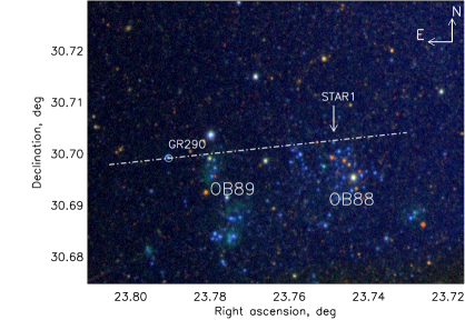
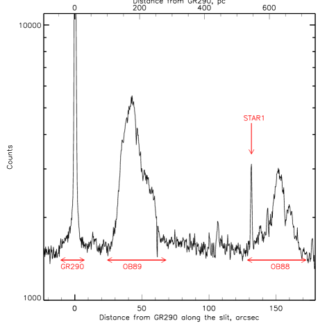
Figure 8: Upper panel: identification chart for GR290. Dash-dotted line shows the slit position during July observations. Lower panel: tracing of the 2-dimensional spectral image obtained of GR 290 in July 2017 along the spatial direction centred on the H$\alpha$ emission line. GR 290 is located at zero point and has a strong and sharply-peaked H$\alpha$ line with asymmetrically extended wings.

H$\alpha$ is present at all three positions. The [S ii] 6717, 6731 Å  lines are absent at Position 1 and the [O iii] 4959, 5007 Å lines are absent at Positions 2 and 3. He i is not detected at Position 2. The spectrum at Position 1 also displays lines of [Fe iii]5270 and [Ar iii]7136.

We used the CLOUDY (version 17.00) photoionization code Ferland et al. (1998, 2017) for revealing the properties of the nebula surrounding the GR 290 star. More than a thousand models were computed varying chemical composition, density and outer radius of the nebula. The parameters of our best CMFGEN model were used to set the luminosity, $T_{\rm eff}$ and spectral energy distribution of the central ionizing source. We adopted a closed spherical geometry of the nebula with the same filling factor as for the star atmosphere.

Two scenarios for the nebular chemical composition were considered. It could be formed from the surrounding material, or from the LBV ejecta. For the first scenario we assumed that the chemical composition of the compact ISM region is as usually found for H II regions, scaled to the metallicity of M 33 at the galactocentric distance of GR 290 ($\mathrm{12+\log(O/H)\simeq 8.15}$, or $Z\simeq 0.3Z_{\odot}$, given the metallicity gradient derived by Rosolowsky & Simon (2008); Bresolin (2011)). We also computed the models for 0.1, 0.2, 0.4 and 0.5 $Z_{\odot}$. In the second scenario we assumed that the compact nebula was formed primarily from LBV ejecta, and we adopted the chemical composition deduced from the CMFGEN model (Table 4).

For each set of abundances, the hydrogen density was varied in the range $\log(n_{H})=1.0-3.6$ and the outer radius was varied in the $R=0.5-6$ pc. We also considered larger densities and radii, but the corresponding models failed completely to fit the observed spectrum.

The aim of the modeling was to reproduce the observed nebular emission lines that are clearly seen in observed spectrum and not predicted by the CMFGEN model ([N ii]6548, 6584; [O iii]4959, 5007; [Fe iii]5270). These lines are assumed to arise in the the circumstellar medium that is photoionized by GR 290. An additional constraint on the model is the absence of the [S ii]6717, 6731 Å. The observed and modeled fluxes of these lines were compared and a chi-square value for each model was computed. The sum of CMFGEN model and CLOUDY model spectra is presented in Fig. 6.

We find that models for a nebula having the same chemical composition as the LBV stellar atmosphere yield chi-square values that are several times smaller than the models in which the alternative set of abundances are used. This result favors the hypothesis that the nebula around GR 290 has been formed primarily from material ejected from the star. Another finding is that only relatively small outer radii yield spectra similar to that observed: for $R>4$ pc the nebular emission lines become much brighter than observed, at any density and chemical abundance. This effect is clearly seen in Fig. 9, where the chi-square distribution for different densities and radii is shown and where the abundances are held constant. Although the values of the chi-squared distribution may vary for different sets of abundances, the general trend is the same.

The minimum chi-square from all the computed models is obtained for an outer radius $R=0.8$ pc and a hydrogen density $n_{\mathrm{H}}=160\ \mathrm{cm^{-3}}$. Unfortunately, the spatial resolution of our observations is limited by the “seeing” ($\sim$1”), which at the distance of M 33 implies that we cannot resolve structures smaller than 4 pc in extension.

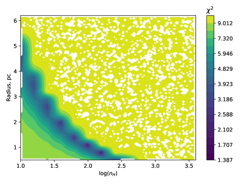
Figure 9: Chi-square distribution for the CLOUDY models with different densities and outer radii. Chemical composition here is the same as for GR 290 best-fit CMFGEN model, but with two times larger abundance of O and Fe. For clarity all values of $\chi^{2}>10$ were changed to 10 in this plot.

All the computed models reproduce approximately the observations if the radius of this nebula does not exceed 4 pc, with a preferred diameter being 2 pc. A larger nebula would produce brighter emission lines than observed, regardless of density and metallicity.

While most of the lines in the models are consistent with the observations, the [O iii]4959, 5007 ones are 2-3 times fainter than observed if we assume that N/O=15 like in the atmosphere of the star. Moreover, such high N/O ratio is inconsistent with the ones for other LBVs (Table 7). This inconsistency could be resolved if the oxygen abundance of the nebula were 3 times greater than the one implied by the CMFGEN model – i.e. if it is N/O=5 as we list in Table 7. The difference between chemical compositions of the nebula and the atmosphere does not contradict the predictions of evolutionary theory. Indeed, according to the predictions of evolutionary tracks (e.g. Groh et al. (2014)) the surface abundance of oxygen rapidly drops by about 1.5 orders of magnitude during the LBV phase, while the nitrogen abundance increases by only two times. At the same time, the nebula may be formed well before LBV stage, during the transition from main sequence towards blue supergiants (Lamers et al. 2001), and therefore may have increased nitrogen and normal (equal to surrounding metallicity) oxygen abundance.

The CLOUDY model only partially recovered the broad [Fe iii]5270 presented in the spectrum of GR 290 (Fig. 6). Probably it is related to the adopted geometry of the model that would require future investigations.

Table 7: Nebular parameters for some LBVs and of GR290.

Name	Galaxy	Type	Max.size	${n_{e}}$	N/O	N/S	(N+O)/H	Ref
			(pc)	($\mathrm{cm^{-3}}$)
AG Car	MW	bipolar	$1.4\times 2$	$820\pm 170$	$6\pm 2$	¡45	$4\times 10^{-4}$	1, 2
P Cyg	MW	spherical	0.2/0.84	600	¿0.16	33	$0.4-3\times 10^{-3}$	1, 2
WRA 751	MW	spherical/bipolar	0.6	200	$3^{+3}_{-1.5}$		$4-4.9\times 10^{-4}$	1, 3
R 127	LMC	bipolar	1.3	$720\pm 90$	$0.9\pm 0.4$	¡34	$3.2\times 10^{-4}$	1, 2
S 119	LMC	spherical/outflow	1.8	$680\pm 170$	$1.9\pm 0.5$	¡78	$3.8\times 10^{-4}$	1, 2
GR 290	M 33		0.8-4	$160^{a}$	$\leavevmode\nobreak\ 5^{b}$	65	$7.3\times 10^{-4}$	this work

Notes: Types and sizes are taken from (1) Weis (2011) while $n_{e}$ and chemical composition are taken from (2) Lamers et al. (2001) and (3) Garcia-Lario et al. (1998). ^a Here we show CLOUDY-estimated $n_{H}$ as $n_{e}$. ^b See the text for the discussion on how we estimated this quantity.

Table 7 presents the comparison of GR 290’s nebula parameters with the ones of four other LBVs belonging to our Galaxy (MW) and Large Magellanic Cloud (LMC). As we can see the sizes of all five nebulae are similar, and the one of GR 290’s nebula is in good agreement with average sizes of LBVs according to Weis (2012). However, $n_{e}$ for GR 290’s nebula is significantly lower, just like the one for WRA 751 (Garcia-Lario et al. 1998).

Fabrika et al. (2005) reported the marginal detection of a circumstellar nebula around GR 290 based on integral field spectroscopy. They found a radial velocity gradient within the nebula of $44\pm 11$ ${\rm km\leavevmode\nobreak\ s^{-1}}$ and an angular size $\sim 9$” in the NE-SW direction. The detection is classified as marginal because, their spectra did not cover the H$\alpha$ spectral region and they did not detect the [O iii] lines, so the results are based on the analysis of the H$\beta$ line profiles alone. However, if real, this region would correspond to material lying intermediate between the compact H II region that we detect (R$\leq$4 pc) in the emission-line spectrum and the material that we are able to resolve at a projected distance of 16-40 pc to the East of GR 290. If this intermediate material reflects an asymmetric ejection, it increases the possibility that the inner compact H II region is also asymmetrical. It is also interesting to note that a preliminary CLOUDY photoionization model indicates that GR 290 could be responsible for producing at least a fraction of the observed [S II] at these distances, with no [O iii]. However, a more detailed analysis of the extended regions requires observations with higher S/N than those we currently present.

5 Conclusions

We present results of long-slit observations obtained with GTC in 2016 of the LBV/WR object GR 290 (Romano’s star). GR 290 lies in a relatively external region of the M 33 galaxy, where metallicity is low compared to Solar values. Fitting CMFGEN models to the stellar spectrum we find a current effective temperature $T_{\rm eff}=27000-30000$ K at a radius $R_{2/3}=27-23{\rm R_{\odot}}$. It’s mass-loss rate is 1.5$\times$10^-5 ${\rm M_{\odot}yr^{-1}}$.

The terminal wind speed ${\mathrm{v}}_{\infty}$=620 ${\rm km\leavevmode\nobreak\ s^{-1}}$ is faster than ever before recorded while the current luminosity $L_{*}=(3.1-3.7)\times$10⁵ ${\rm L_{\odot}}$ is the lowest ever deduced. The remaining parameters of the 2016 observation fall within the ranges of values obtained at previous epochs as described in Polcaro et al. (2016) We also confirm previous conclusions that the stellar wind is overabundant in He and N and underabundant in C and O.

We find the star in GR 290 to be surrounded by an unresolved compact H II region with dimensions $\leq$4 pc, and having chemical abundances that are consistent with those derived from the stellar wind lines. Hence, this compact H II region appears to be largely composed of material ejected from the star. In addition, we find partially resolved emission from a more extended ISM region which appears to be asymmetrical, with a larger extent to the East ($16-40$ pc) than to the West. If associated with GR 290, this more extended structure would suggest that GR 290 has undergone significant mass-loss over the past 10⁴-10⁵ years.

The luminosity and effective temperature of GR 290 allow us to place it on the HRD and estimate its mass. Using the Brott et al. (2011) non-rotating evolutionary grid, $M\sim 40-50\leavevmode\nobreak\ {\rm M_{\odot}}$, while with the Chieffi & Limongi (2013) tracks its mass is $\sim$60 ${\rm M_{\odot}}$. The enhanced He and N chemical abundances, along with deficiencies in C and O derived from the CMFGEN models indicate that the surface layers of GR 290 contain significant amounts of nuclear processed material, such as would be expected for a star that has left the Main Sequence and is becoming a WR star (Langer et al. 1994). Adding this to the recent LBV-like eruptive behavior and to the presence of a compact H II region also having altered chemical abundances with respecto to typical H II regions, one is led to conclude that GR 290 is in an advanced stage of evolution, either nearing the end of its core H-burning phase or in later phases.

There are now a number of reported supernova (SNIIn) events that have been observed in extragalactic regions where there has been a massive ejection of material prior to the SN event – often within 10 years – and which is believed to have arisen in an LBV (Foley et al. 2007; Smith et al. 2007, 2011; Smith 2007; Pastorello et al. 2008; Dessart et al. 2011). Thus, given the apparent late evolutionary state of GR 290, it is a good candidate to be a progenitor of a similar event sometime in the future.

6 Acknowledgements

We dedicate this publication to the memory of our dear colleague Vito Francesco Polcaro, who passed away shortly before the final acceptance of the paper.

Dr. Vito Francesco Polcaro passed away on February 11, 2018 in Roma. Besides GR 290, Dr. Polcaro prompted many relevant investigations of hot luminous stars, X-ray counterparts, and circumstellar nebulae, best exploiting in particular the performances of medium and small telescopes. He inspired amateurs to participate in the photometric monitoring of topical objects. Last years Dr. Polcaro has been very active in the field of archeoastronomy, and organized campaigns in paleolithic sites and conferences gathering astronomers and archeologists.

We would like to thank the anonymous referee for a helpful and insightful report. We thank the GTC observatory staff for obtaining the spectra and Antonio Cabrera-Lavers for guidance in processing the observations. GK acknowledges support from CONACYT grant 252499 and thanks Ulises Amaya for computer support. OM acknowledges Russian Foundation for Basic Research grant 16-02-00148 and AV ČR project RVO:67985815. OE acknowledges Russian Foundation for Basic Research grant 18-02-00976.

References

- Abolmasov (2011) Abolmasov, P. 2011, New A, 16, 421
- Afanasiev & Moiseev (2005) Afanasiev, V. L. & Moiseev, A. V. 2005, Astronomy Letters, 31, 194
- Bresolin (2011) Bresolin, F. 2011, ApJ, 730, 129
- Brott et al. (2011) Brott, I., de Mink, S. E., Cantiello, M., et al. 2011, A&A, 530, A115
- Chieffi & Limongi (2013) Chieffi, A. & Limongi, M. 2013, ApJ, 764, 21
- Clark et al. (2012) Clark, J. S., Castro, N., Garcia, M., et al. 2012, A&A, 541, A146
- Conti (1984) Conti, P. S. 1984, in IAU Symposium, Vol. 105, Observational Tests of the Stellar Evolution Theory, ed. A. Maeder & A. Renzini, 233
- Dessart et al. (2011) Dessart, L., Hillier, D. J., Livne, E., et al. 2011, MNRAS, 414, 2985
- Ekström et al. (2012) Ekström, S., Georgy, C., Eggenberger, P., et al. 2012, A&A, 537, A146
- Fabrika et al. (2005) Fabrika, S., Sholukhova, O., Becker, T., et al. 2005, A&A, 437, 217
- Ferland et al. (2017) Ferland, G. J., Chatzikos, M., Guzmán, F., et al. 2017, Revista Mexicana de Astronomiá y Astrofiśica, 53, 385
- Ferland et al. (1998) Ferland, G. J., Korista, K. T., Verner, D. A., et al. 1998, PASP, 110, 761
- Foley et al. (2007) Foley, R. J., Smith, N., Ganeshalingam, M., et al. 2007, ApJ, 657, L105
- Galleti et al. (2004) Galleti, S., Bellazzini, M., & Ferraro, F. R. 2004, A&A, 423, 925
- Garcia-Lario et al. (1998) Garcia-Lario, P., Riera, A., & Manchado, A. 1998, A&A, 334, 1007
- Georgiev et al. (2011) Georgiev, L., Koenigsberger, G., Hillier, D. J., et al. 2011, AJ, 142, 191
- Gräfener et al. (2012) Gräfener, G., Owocki, S. P., & Vink, J. S. 2012, A&A, 538, A40
- Groh et al. (2009) Groh, J. H., Hillier, D. J., Damineli, A., et al. 2009, ApJ, 698, 1698
- Groh et al. (2013a) Groh, J. H., Meynet, G., & Ekström, S. 2013a, A&A, 550, L7
- Groh et al. (2014) Groh, J. H., Meynet, G., Ekström, S., & Georgy, C. 2014, A&A, 564, A30
- Groh et al. (2013b) Groh, J. H., Meynet, G., Georgy, C., & Ekström, S. 2013b, A&A, 558, A131
- Hillier & Miller (1998) Hillier, D. J. & Miller, D. L. 1998, ApJ, 496, 407
- Hillier & Miller (1999) Hillier, D. J. & Miller, D. L. 1999, ApJ, 519, 354
- Humphreys & Davidson (1994) Humphreys, R. M. & Davidson, K. 1994, PASP, 106, 1025
- Humphreys & Sandage (1980) Humphreys, R. M. & Sandage, A. 1980, ApJS, 44, 319
- Humphreys et al. (2014) Humphreys, R. M., Weis, K., Davidson, K., Bomans, D. J., & Burggraf, B. 2014, ApJ, 790, 48
- Humphreys et al. (2016) Humphreys, R. M., Weis, K., Davidson, K., & Gordon, M. S. 2016, ApJ, 825, 64
- Ivanov et al. (1993) Ivanov, G. R., Freedman, W. L., & Madore, B. F. 1993, ApJS, 89, 85
- Koenigsberger et al. (2014) Koenigsberger, G., Morrell, N., Hillier, D. J., et al. 2014, AJ, 148, 62
- Kurtev et al. (2001) Kurtev, R., Sholukhova, O., Borissova, J., & Georgiev, L. 2001, Rev. Mexicana Astron. Astrofis., 37, 57
- Lamers & Cassinelli (1999) Lamers, H. J. G. L. M. & Cassinelli, J. P. 1999, Introduction to Stellar Winds, 452
- Lamers et al. (2001) Lamers, H. J. G. L. M., Nota, A., Panagia, N., Smith, L. J., & Langer, N. 2001, ApJ, 551, 764
- Langer et al. (1994) Langer, N., Hamann, W.-R., Lennon, M., et al. 1994, A&A, 290, 819
- Magrini et al. (2010) Magrini, L., Stanghellini, L., Corbelli, E., Galli, D., & Villaver, E. 2010, A&A, 512, A63
- Martayan et al. (2016) Martayan, C., Lobel, A., Baade, D., et al. 2016, A&A, 587, A115
- Maryeva & Abolmasov (2010) Maryeva, O. & Abolmasov, P. 2010, Rev. Mexicana Astron. Astrofis., 46, 279
- Maryeva & Abolmasov (2012) Maryeva, O. & Abolmasov, P. 2012, MNRAS, 419, 1455
- Massey et al. (1995) Massey, P., Armandroff, T. E., Pyke, R., Patel, K., & Wilson, C. D. 1995, AJ, 110, 2715
- Meynet et al. (2011) Meynet, G., Georgy, C., Hirschi, R., et al. 2011, Bulletin de la Societe Royale des Sciences de Liege, 80, 266
- Meynet & Maeder (2005) Meynet, G. & Maeder, A. 2005, A&A, 429, 581
- Pastorello et al. (2008) Pastorello, A., Quimby, R. M., Smartt, S. J., et al. 2008, MNRAS, 389, 131
- Polcaro et al. (2003) Polcaro, V. F., Gualandi, R., Norci, L., Rossi, C., & Viotti, R. F. 2003, A&A, 411, 193
- Polcaro et al. (2016) Polcaro, V. F., Maryeva, O., Nesci, R., et al. 2016, AJ, 151, 149
- Polcaro et al. (2011) Polcaro, V. F., Rossi, C., Viotti, R. F., et al. 2011, AJ, 141, 18
- Puls et al. (1996) Puls, J., Kudritzki, R.-P., Herrero, A., et al. 1996, A&A, 305, 171
- Romano (1978) Romano, G. 1978, A&A, 67, 291
- Rosolowsky & Simon (2008) Rosolowsky, E. & Simon, J. D. 2008, ApJ, 675, 1213
- Sander et al. (2017) Sander, A. A. C., Hamann, W.-R., Todt, H., Hainich, R., & Shenar, T. 2017, A&A, 603, A86
- Sholukhova et al. (2002) Sholukhova, O., Zharova, A., Fabrika, S., & Malinovskii, D. 2002, in Astronomical Society of the Pacific Conference Series, Vol. 259, IAU Colloq. 185: Radial and Nonradial Pulsationsn as Probes of Stellar Physics, ed. C. Aerts, T. R. Bedding, & J. Christensen-Dalsgaard, 522
- Sholukhova et al. (1997) Sholukhova, O. N., Fabrika, S. N., Vlasyuk, V. V., & Burenkov, A. N. 1997, Astronomy Letters, 23, 458
- Sholukhova et al. (2011) Sholukhova, O. N., Fabrika, S. N., Zharova, A. V., Valeev, A. F., & Goranskij, V. P. 2011, Astrophysical Bulletin, 66, 123
- Smith (1968) Smith, L. F. 1968, MNRAS, 138, 109
- Smith et al. (1996) Smith, L. F., Shara, M. M., & Moffat, A. F. J. 1996, MNRAS, 281, 163
- Smith (2007) Smith, N. 2007, in American Institute of Physics Conference Series, Vol. 937, Supernova 1987A: 20 Years After: Supernovae and Gamma-Ray Bursters, ed. S. Immler, K. Weiler, & R. McCray, 163–170
- Smith et al. (2011) Smith, N., Li, W., Filippenko, A. V., & Chornock, R. 2011, MNRAS, 412, 1522
- Smith et al. (2007) Smith, N., Li, W., Foley, R. J., et al. 2007, ApJ, 666, 1116
- Szeifert (1996) Szeifert, T. 1996, in Liege International Astrophysical Colloquia, Vol. 33, Liege International Astrophysical Colloquia, ed. J. M. Vreux, A. Detal, D. Fraipont-Caro, E. Gosset, & G. Rauw, 459
- van der Hucht et al. (1981) van der Hucht, K. A., Conti, P. S., Lundstrom, I., & Stenholm, B. 1981, Space Sci. Rev., 28, 227
- Vink (2012) Vink, J. S. 2012, in Astrophysics and Space Science Library, Vol. 384, Eta Carinae and the Supernova Impostors, ed. K. Davidson & R. M. Humphreys, 221
- Viotti et al. (2007) Viotti, R. F., Galleti, S., Gualandi, R., et al. 2007, A&A, 464, L53
- Viotti et al. (2006) Viotti, R. F., Rossi, C., Polcaro, V. F., et al. 2006, A&A, 458, 225
- Walborn et al. (2017) Walborn, N. R., Gamen, R. C., Morrell, N. I., et al. 2017, AJ, 154, 15
- Weis (2011) Weis, K. 2011, in IAU Symposium, Vol. 272, Active OB Stars: Structure, Evolution, Mass Loss, and Critical Limits, ed. C. Neiner, G. Wade, G. Meynet, & G. Peters, 372–377
- Weis (2012) Weis, K. 2012, in Astronomical Society of the Pacific Conference Series, Vol. 465, Proceedings of a Scientific Meeting in Honor of Anthony F. J. Moffat, ed. L. Drissen, C. Robert, N. St-Louis, & A. F. J. Moffat, 213
- Wolf (1989) Wolf, B. 1989, A&A, 217, 87
- Zharova et al. (2011) Zharova, A., Goranskij, V., Sholukhova, O. N., & Fabrika, S. N. 2011, Peremennye Zvezdy Prilozhenie, 11, 11