Palindromic sequences of the Markov spectrum

Abstract.

We study the periods of Markov sequences, which are derived from the continued fraction expression of elements in the Markov spectrum. This spectrum is the set of minimal values of indefinite binary quadratic forms that are specially normalised. We show that the periods of these sequences are palindromic after a number of circular shifts, the number of shifts being given by Stern’s diatomic sequence.

Introduction

In this paper we state and prove a general result on the construction of palindromic sequences. These include sequences relating to the Markov spectrum. The Markov spectrum is the set of numbers

(1) $$\inf\limits_{\mathbb{Z}^{2}\setminus\{(0,0)\}}\bigg{|}\frac{\sqrt{\Delta}}{f}\bigg{|}$$

for all binary quadratic forms $f$ with positive discriminant $\Delta(f)$.

A. Markov showed in his papers [7, 8] that for any element of the Markov spectrum less than $3$ there exists a sequence of positive integers $(a_{1},\ldots,a_{2n})$ such that

(2) $$\inf\limits_{\mathbb{Z}^{2}\setminus\{(0,0)\}}\bigg{|}\frac{\sqrt{\Delta}}{f}\bigg{|}=[(a_{1},a_{2},\ldots,a_{2n})]+[0;\overline{(a_{1},\ldots,a_{2n})}],$$

where $[(a_{1},a_{2},\ldots,a_{2n})]$ is the infinite continued fraction with period $(a_{1},a_{2},\ldots,a_{2n})$. In this paper we denote the reverse of the sequence $(a_{1},\ldots,a_{2n})$ by $\overline{(a_{1},\ldots,a_{2n})}$. Equation (2) is known as the Perron identity, going back to [9].

It is known, see for example the books by T. Cusick and M. Flahive [3], and M. Aigner [1], that the numbers $a_{i}$ satisfy the following

• $a_{i}\in\{1,2\}$

• $a_{1}=a_{2}=2$, $a_{2n}=a_{2n-1}=1$

• The subsequence $w{=}(a_{3},\ldots,a_{2n-2})$ is palindromic, i.e. $w=\overline{w}$.

One can find work on Markov numbers in relation to other branches of mathematics in the following articles: [4], [11], [10], [5], [13].

The sequences for which expression (1) is less than $3$, henceforth called Markov sequences, may be constructed by concatenation of the sequences $(2,2)$, and $(1,1)$ (see Definition 1.5 below). This follows as a corollary of the work of H. Cohn [2], specifically found in [1, Theorem 4.7].

We show in Theorem 1.13 that any sequence constructed in the same way as Markov sequences are evenly palindromic, that is, after some number of circular shifts the sequence is palindromic. The number of circular shifts is given by Stern’s diatomic sequence, an exposition of which can be found in the paper of I. Urbiha, [14].

In the forthcoming paper [6], we use Theorem 1.13 to show that there is a generalisation of Markov numbers coming from the graph structure in Definition 1.5.

Organisation of the Paper

In Section 1 we give a background for Markov sequences, and give the necessary definitions for our main result, Theorem 1.13.

In Section 2 we prove Theorem 1.13.

Acknowledgements. The author is grateful to O. Karpenkov for his constant attention to this work.

1. Some history and background

In this section we give the necessary definitions and background for the main result of the paper, Theorem 1.13.

1.1. The Markov spectrum

In this subsection we define the Markov spectrum in terms of binary quadratic forms and sequences of positive integers. We start with the following definition.

Definition 1.1.

Let $f$ be a binary quadratic form with positive discriminant $\Delta$. The Markov element of $f$ is defined to be

$$M(f)=\inf\limits_{\mathbb{Z}^{2}\setminus\{(0,0)\}}\left|\frac{f}{\sqrt{\Delta}}\right|.$$

The Markov spectrum is the set of values $1/M(f)$ for all such forms $f$.

For a sequence of positive integers $a_{1},\ldots,a_{n}$, let

$$[a_{1};a_{2}:\ldots:a_{n}]$$

denote the continued fraction of $a_{1},\ldots,a_{n}$. We give an alternative definition of the Markov spectrum.

Definition 1.2.

Let $A$ be a doubly infinite sequence of positive integers

$$A=\ldots,a_{-2},a_{-1},a_{0},a_{1},a_{2},\ldots.$$

Define $M(A)$, the Markov element of $A$, by

(3) $$\frac{1}{M(A)}=\inf\limits_{i\in\mathbb{Z}}\left(a_{i}+[0;a_{i+1}:a_{i+2}:\ldots]+[0;a_{i-1}:a_{i-2}:\ldots]\right).$$

The right hand side of Equation (3) is known as the Perron identity. The set of values $1/M(A)$ for all such sequences $A$ is called the Markov spectrum.

Remark 1.3.

Definitions 1.1 and 1.1 are equivalent, see [9]. The sequences $A$ for which $M(A)>1/3$ are purely periodic and consist solely of the integers $1$, and $2$. We refer to these sequences as Markov sequences.

1.2. Graph structure of Markov sequences

We give an alternative definition of Markov sequences.

Definition 1.4.

Let $\mathbb{Z}^{\infty}$ be the set of finite sequences of integer elements. Consider the binary operation $\oplus$ on $\mathbb{Z}^{\infty}$ defined as

$$(a_{1},\ldots,a_{n})\oplus(b_{1},\ldots,b_{m})=(a_{1},\ldots,a_{n},b_{1},\ldots,b_{m}).$$

We call this the concatenation of sequences $(a_{1},\ldots,a_{n})$ and $(b_{1},\ldots,b_{m})$. Let also for $A$, $B$, $C\in\mathbb{Z}^{\infty}$

$$\mathcal{L}_{\oplus}(A,B,C)=(A,A\oplus B,B),\ \ \mathcal{R}_{\oplus}(A,B,C)=(B,B\oplus C,C).$$

Definition 1.5.

We define $\mathcal{G}(\mathbb{Z}^{\infty},\oplus,x)$ to be the directed graph whose vertices are elements in $({\mathbb{Z}^{\infty}})^{3}$, and containing the vertex $x$. The vertices $v$, $w\in{\mathbb{Z}^{\infty}}^{3}$ are connected by an edge $(v,w)$ if either

$$w=\mathcal{L}_{\oplus}(v),\ \ \ \mbox{or}\ \ \ w=\mathcal{R}_{\oplus}(v).$$

For $A$, $B\in\mathbb{Z}^{\infty}$ we write

$$\mathcal{G}(\mathbb{Z}^{\infty},\oplus,(A,A\oplus B,B)=\mathcal{G}_{A,B}.$$

Remark 1.6.

The graph $\mathcal{G}_{(1,1),(2,2)}$ is called the graph of general Markov sequences and contains all Markov sequences, see [3, 6].

Definition 1.7.

Let $v$ be the vertex $(A,A\oplus B,B))\in\mathcal{G}_{A,B}$. Let $w$ be a vertex in $\mathcal{G}_{A,B}$. We say that $(\alpha_{1},\ldots,\alpha_{2n})$ is a path from $v$ to $w$ if

$$w=\mathcal{L}_{\oplus}^{\alpha_{2n}}\mathcal{R}_{\oplus}^{\alpha_{2n-1}}\ldots\mathcal{L}_{\oplus}^{\alpha_{2}}\mathcal{R}_{\oplus}^{\alpha_{1}}(v).$$

We define the $N$-th level in $\mathcal{G}_{A,B}$ to be all vertices $w$ such that the path $(\alpha_{1},\ldots,\alpha_{2n})$ from $v$ to $w$ satisfies $\sum_{i=1}^{2n}\alpha_{i}=N.$

We give an ordering for the vertices in each level of $\mathcal{G}_{A,B}$.

Definition 1.8.

For positive integers $n$, $m$, $\alpha_{1},\ldots,\alpha_{2n}$, $\beta_{1},\ldots,\beta_{2m}$ satisfying $\sum_{i=1}^{2n}\alpha_{i}=\sum_{i=1}^{2m}\beta_{i}$, let $w_{1}$, $w_{2}$ be two vertices in $\mathcal{G}_{A,B}$ with

$$w_{1}=\mathcal{L}_{\oplus}^{\alpha_{2n}}\mathcal{R}_{\oplus}^{\alpha_{2n-1}}\ldots\mathcal{L}_{\oplus}^{\alpha_{2}}\mathcal{R}_{\oplus}^{\alpha_{1}}(v)\ \mbox{and}\ w_{2}=\mathcal{L}_{\oplus}^{\beta_{2m}}\mathcal{R}_{\oplus}^{\beta_{2m-1}}\ldots\mathcal{L}_{\oplus}^{\beta_{2}}\mathcal{R}_{\oplus}^{\beta_{1}}(v).$$

Define an ordering of vertices by

$$w_{1}\prec w_{2}$$

if either

$$\alpha_{i} =\beta_{i},\mbox{ for}\ i=1,\ldots,2k{-}1,\ k<m,n\ \mbox{and }\alpha_{2k}>\beta_{2k},\ \mbox{or}$$

$$\alpha_{i} =\beta_{i},\mbox{ for}\ i=1,\ldots,2k,\ k<m,n\ \mbox{and }\alpha_{2k+1}<\beta_{2k+1}.$$

Definition 1.9.

Let the pair $(\mathcal{G}_{A,B},\prec)$ be the graph $\mathcal{G}_{A,B}$ where each level $n$ is ordered

$$w_{1}\prec w_{2}\prec\ldots\prec w_{2^{n}}.$$

We define the sequence $(S(i))_{i=0}^{\infty}$.

Definition 1.10.

For two sequences $A$, and $B$ let

$$S(0)=A,\ \ S(1)=B\ \ S(2)=A\oplus B.$$

For $n>1$, and $1\leq i\leq 2^{n-1}$ let $S(2^{n-1}{+}i)$ be the central element of the $i$-th vertex in the $n$-th level of the ordered graph $(\mathcal{G}_{A,B},\prec)$. We call $(S(i))$ the ordered Markov sequences for $A$ and $B$.

When we want to specify the sequences $A$, and $B$ we write

$$S_{A,B}(n).$$

Example.

We have

$$S_{(a,a),(b,b)}(14)=(a,a,b,b,a,a,b,b,b,b,a,a,b,b,b,b).$$

For $(a,b)=(1,2)$ we have for all $i\geq 1$ that $M(S_{(a,a),(b,b)}(i))>1/3$.

Definition 1.11.

Let $\Lambda=(\lambda_{1},\ldots,\lambda_{2n})$, $\Gamma=(\gamma_{1},\ldots,\gamma_{2n+1})$. We call $\Lambda$ and $\Gamma$ evenly palindromic and oddly palindromic respectively if there exists $k_{1}$, $k_{2}\in\mathbb{Z}$ such that for all $i\in\mathbb{Z}$ we have

$$\lambda_{k_{1}+i\mod 2n} =\lambda_{k_{1}-i-1\mod 2n},$$

$$\gamma_{k_{2}+i+1\mod 2n+1} =\gamma_{k_{2}-i-1\mod 2n+1}.$$

Definition 1.12.

Let $d_{0}=0$ and $d_{1}=1$, and for all positive integers $n>1$ set

$$d_{2n}=d_{n},\ \ \ \ d_{2n{-}1}=d_{n}{+}d_{n{-}1}.$$

The sequence $(d_{n})_{n\geq 0}$ is called Stern’s diatomic sequence.

We give the main theorem of this paper.

Theorem 1.13.

Let $A$ and $B$ be two palindromic sequences of positive integers. Let $n$ be a positive integer, and let $N$ be the sum of powers of $A$’s and $B$’s in $S_{A,B}(n)$. Let $\Lambda_{i}\in\{A,B\}$ such that

$$S_{A,B}(n)=\Lambda_{1}\ldots\Lambda_{N}.$$

Then the following sequences are palindromic

$$\begin{cases}\Lambda_{\lceil d_{n}/2\rceil}\Lambda_{\lceil d_{n}/2\rceil+1}\ldots\Lambda_{N}\Lambda_{1}\ldots\Lambda_{\lceil d_{n}/2\rceil-1},&d_{n}\mbox{ even},\\ \lceil\Lambda_{\lceil d_{n}/2\rceil}\rceil\Lambda_{\lceil d_{n}/2\rceil+1}\ldots\Lambda_{N}\Lambda_{1}\ldots\Lambda_{\lceil d_{n}/2\rceil-1}\lfloor\Lambda_{\lceil d_{n}/2\rceil}\rfloor,&d_{n}\mbox{ odd}.\end{cases}$$

2. Proof of Theorem 1.13

In this section we prove Theorem 1.13. We start by stating Proposition 2.2, which deals with the majority of the proof. Subsections 2.1 through 2.4 deal with proving this lemma, while the final proof of Theorem 1.13 is in Subsection 2.5.

2.1. Alternative definition for $S(n)$

We state Proposition 2.2, which is central to our proof of Theorem 1.13. We then give an alternative definition for the sequences $(S(n))$ in Proposition 2.4, defining each $S(n)$ by concatenations of previous terms in $(S(n))$. We start by defining circular shifts of Markov sequences.

Definition 2.1.

Let $A=(a_{0},\ldots,a_{n})$ be a sequence of positive integers, and for each $0\leq i<n$ define the operation

$$C_{i}(A)=(a_{i},\ldots,a_{n},a_{1},\ldots,a_{i-1}).$$

Then $C_{i}(A)$ is called the $i$-th circular shift of $A$.

Proposition 2.2.

Every sequence $S(i)$ is evenly palindromic. Moreover, we have that the sequence

$$C_{d_{i}}(S(i))$$

is palindromic, where $d_{i}$ is the $i$-th element in Stern’s diatomic sequence.

Example.

$S_{(a,a),(b,b)}(3)=(a,a,a,a,b,b)$, and $d_{3}=2$. Then

$$C_{2}(S_{(a,a),(b,b)}(3))=(a,a,b,b,a,a).$$

We define a sequence $(a(j))_{j\geq 0}$ which simplifies notation of $(S(j))$.

Definition 2.3.

Let $a(1){=}a(2){=}1$, and for all positive integers $j>1$ set

$$a(2j)=a(j)\ \ \ \ a(2j{-}1)=j.$$

The sequence $(a(j))_{j\geq 0}$ is A003602 in [12]. Denote by $(a^{*}(j))$ the sequence defined

$$a^{*}(j)=\begin{cases}a(j),&\mbox{if }j>1,\\ 0,&\mbox{if }j=1.\\ \end{cases}$$

For the $a(j)$-th element in the sequence $(S(n))$, we write $S\circ a(j)$.

Example.

The first 10 elements of $(a(j))$ and $(d_{j})$ are given

$$(a(j))_{1}^{10} =(1,1,2,1,3,2,4,1,5,3),$$

$$(d_{j})_{0}^{9} =(0,1,1,2,1,3,2,3,1,4).$$

Figure 1 shows the symmetry in Stern’s diatomic sequence.

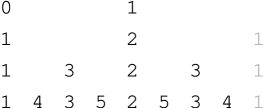
Figure 1. The first entries in Stern’s diatomic sequence.

Proposition 2.4.

Let $a>b$ be positive integers, and let

$$S(0)=A,\ \ S(1)=B,\ \ S(2)=A\oplus B.$$

The following definitions of the sequence $(S(j))_{j>2}$ are equivalent.

• For $n>1$ and $1\leq i\leq 2^{n-1}$, define $S(2^{n-1}{+}i)$ to be the central element of the $i$-th vertex in the $n$-th level of the graph

  $$\mathcal{G}(\mathbb{Z}^{\infty},\oplus,(A,A\oplus B,B).$$

• Define

  $$S(2j) =S(j)\oplus S\circ a(j),\ \mbox{and}$$

  $$S(2j{-}1) =S\circ a^{*}(j{-}1)\oplus S(j).$$

Remark 2.5.

Proposition 2.4 gives us an alternative definition for the sequences $(S(n))$.

For Proposition 2.4 we first prove the following lemma.

Lemma 2.6.

For $m=2k>2$ the following equations hold

$$S(2^{n-2}{+}k) =S(a^{*}(2^{n-1}{+}m{-}1)),\ S(2^{n-1}{+}2k)=S(2^{n-1}{+}m),$$

$$S(2(2^{n-2}{+}k)) =S(2^{n-1}{+}m),\ S(a(2^{n-2}{+}k))=S(a(2^{n-1}{+}m)).$$

For $m=2k{-}1>2$ the following equations hold

$$S(a^{*}(2^{n-2}{+}k{-}1)) =S(a^{*}(2^{n-1}{+}m{-}1)),\ S(2^{n-2}{+}k)=S(a(2^{n-1}{+}m)).$$

$$S(2(2^{n-2}{+}k){-}1) =S(2^{n-1}{+}m),\ \ S(2(2^{n-2}{+}k){-}1)=S(2^{n-1}{+}m),$$

Proof.

For each case the equations follow from direct application of Definition 2.3. ∎

Proof of Proposition 2.4.

We prove this by induction on the levels of the graph of Markov sequences. The base of induction is given by

$$S(3) =S(0)\oplus S(2)=S\circ a^{*}(1)\oplus S(2),\ \mbox{and}$$

$$S(4) =S(2)\oplus S(1)=S(2)\oplus S\circ a(2).$$

Next we assume that the hypothesis is true for every $S(j)$ up the $n{-}1$-th level, that is to say, we have for $i=1,\ldots,2^{n-1}$ that

(4) $$S(2^{n-1}{+}i)=\begin{cases}S(2(2^{n-2}{+}k)),&\mbox{if }i=2k,\\ S(2(2^{n-2}{+}k){-}1),&\mbox{if }i=2k-1.\end{cases}$$

By definition of $(S(j))$ we have that

$$S(2(2^{n-2}{+}k))=S(2^{n-2}{+}k)\oplus S\circ a(2^{n-2}{+}k),\ \ \mbox{and}$$

$$S(2(2^{n-2}{+}k){-}1)=S\circ a^{*}(2^{n-2}{+}k{-}1))\oplus S(2^{n-2}{+}k).$$

From the induction hypothesis we have

$$S(2(2^{n-1}{+}m)) =S(2^{n-1}{+}m)\oplus S\circ a(2^{n-1}{+}m),$$

$$S(2(2^{n-1}{+}m){-}1) =S\circ a^{*}(2^{n-1}{+}m{-}1)\oplus S(2^{n-1}{+}m).$$

We take both an $\mathcal{L}_{\oplus}$ and an $\mathcal{R}_{\oplus}$ operation on either case in Equation (4). For $i=2k$ we have from Lemma 2.6 that

$$\mathcal{L}_{\oplus}(S(2^{n-1}{+}i)) =S(2^{n-2}{+}k)\oplus S(2^{n-1}{+}2k)$$

$$=S\circ a^{*}(2^{n-1}{+}m{-}1)\oplus S(2^{n-1}{+}m),$$

$$\mathcal{R}_{\oplus}(S(2^{n-1}{+}i)) =S(2(2^{n-2}{+}k))\oplus S\circ a(2^{n-2}{+}k)$$

$$=S(2^{n-1}{+}m)\oplus S\circ a(2^{n-1}{+}m).$$

For the case where $i=2k-1$ is similar after application of Lemma 2.6. All cases for the element in the $n$-th level coming from Equation (4) are covered, completing the proof. ∎

Definition 2.7.

The length of the sequence $S(n)$ is denoted $|S(n)|$.

Remark 2.8.

From Proposition 2.4 we have since $|S(0)|=|S(1)|$ that

$$|S(2n)| =|S(n)|+|S\circ a(n)|,\ \mbox{and}$$

$$|S(2n{-}1)| =|S(a(n{-}1))|+|S(n)|.$$

2.2. Symmetry of construction of sequences $S((n))$

We use the symmetry of the graph $\mathcal{G}_{a,b},\prec$ and of Stern’s diatomic sequence to prove Lemma 2.12 that significantly shortens the proof of Proposition 2.2. For this we need the following short lemmas.

Lemma 2.9.

For $k\geq 2$ we have

$$|S(k)|=|S\circ a(k)|+|S\circ a(k{-}1)|.$$

Proof.

We prove this lemma by induction. First we have

$$|S(2)|=4=2|S(1)|=|S\circ a(2)|+|S\circ a(1)|.$$

Assume $|S(k)|=|S\circ a(k)|{+}|S\circ a(k{-}1)|$ for all $k=2,\ldots,N{-}1$, for some $N\in\mathbb{Z}$. We have two cases:

• If $N=2m$, then

  $$|S(2m)| =|S(m)|+|S\circ a(m)|$$

  $$=|S\circ a(2m{-}1)|+|S\circ a(2m)|$$

  $$=|S\circ a(N{-}1)|+|S\circ a(N)|.$$

• The $N=2m-1$ case is similar. This concludes the proof.

∎

Lemma 2.10.

For $k\geq 1$ we have that

$$|S\circ a(k)|=2d_{k}.$$

Proof.

We prove this by induction again. First we have

$$|S\circ a(2)|=|S\circ a(1)|=2=2d_{1}=2d_{2}.$$

Assume $|S\circ a(k)|=2d_{k}$ for all $k=1,\ldots,N{-}1$, for some positive integer $N$. We have two cases:

• If $N=2m$, then $d_{2m}=d_{m}$, and $|S\circ a(2m)|=|S\circ a(m)|$. So

  $$2d_{N}=|S\circ a(N)|,$$

  which happens if and only if

  $$2d_{m}=|S\circ a(m)|.$$

• The $N=2m{-}1$ case is proved similarly. This concludes the proof.

∎

Lemma 2.11.

For a positive odd integer $k=k_{1}$, let $i\in\mathbb{Z}$ be such that the numbers

$$k_{j}=\frac{k_{j-1}+1}{2},\ j=1,\ldots,i,$$

are positive integers, with $k_{i}$ even. Let $k_{i+1}=k_{i}/2$. Then

$$\frac{|S(k_{i+1})|}{2}=d_{k{-}1}.$$

Proof.

From Definition 2.3 and Lemma 2.10 we have $a(2k_{i+1}{-}1){=}k_{i+1}$, $a(k_{i}{-}1){=}k_{i+1}$, and $d_{k_{i}{-}1}{=}d_{k_{2}{-}1}{=}\ldots{=}d_{k_{i}{-}1}$. Hence $S(k_{i+1}){=}S\circ a(k_{i}{-}1)$ and so

$$|S\circ a(k_{i}{-}1)|=2d_{k{-}1}.$$

∎

Lemma 2.12.

Let $n>1$. For $i=1,\ldots,2^{n-1}$ define the integers

$$k^{\prime}=6\cdot 2^{n-2}{+}i{-}1\ \mbox{ and }\ k^{\prime\prime}=6\cdot 2^{n-2}{-}i{+}1.$$

Then we have

$$\frac{\left|S(k^{\prime}+1)\right|}{2}-d_{k^{\prime}+1}=d_{k^{\prime\prime}}.$$

Remark 2.13.

Let $f$ be a function taking a sequence $S_{A,B}(k)$ to $S_{B,A}(k)$. Due to the symmetry of the Definition 1.10 we have that, for every $k>2$, there is a number $l$ such that

$$S(k)=\overline{f(S(m))}.$$

Lemma 2.12 says that if $k=6\cdot 2^{n-2}+i$ for positive integers $n$ and $i=1,\ldots,2^{n-1}$, then

$$m=6\cdot 2^{n-2}-i+1.$$

Proof of Lemma 2.12.

We have that $k^{\prime}{+}1=a(2(k^{\prime}{+}1){-}1)$ from Definition 2.3. Using Lemma 2.10 we then have

$$\frac{|S(k^{\prime}+1)|}{2}=\frac{|S\circ a(2(k^{\prime}+1)-1)|}{2} =d_{2(k^{\prime}+1)-1}$$

$$=d_{k^{\prime}+1}+d_{k^{\prime}}.$$

It remains to show that

$$d_{k^{\prime}}=d_{k^{\prime\prime}},$$

but this follows from the symmetry seen in Figure 1. ∎

2.3. Alternate form for Markov sequences

In the proof of Proposition 2.2 we will use different formulae for Markov sequences than in Proposition 2.4, and we set these down in the following two Lemmas.

Lemma 2.14.

For a positive even integer $k=k_{1}$, let $i\in\mathbb{Z}$ be such that the numbers

$$k_{j}=\frac{k_{j-1}}{2},\ j=1,\ldots,i,$$

are positive integers, and $k_{i}$ is odd. Let $k_{i+1}=(k_{i}{+}1)/2$. Then

$$S(k)=S\circ a^{*}(k_{i+1}{-}1)\oplus S(k_{i+1})^{i},$$

where the power $i$ indicates a sequence concatenated $i$ times.

Proof.

Through application of Proposition 2.4 we have that

$$S(k)=S(k_{2})\oplus S\circ a(k_{2})=S(k_{i})\oplus S\circ a(k_{i})^{i-1}.$$

Since $k_{i}=2k_{i+1}{-}1$, we have that

$$S(k_{i})=S\circ a^{*}(k_{i+1}{-}1)\oplus S(k_{i+1}).$$

and so

$$S(k)=S\circ a^{*}(k_{i+1}{-}1)\oplus S(k_{i+1})^{i},$$

proving the lemma. ∎

Lemma 2.15.

For a positive odd integer $k=k_{1}$, let $i\in\mathbb{Z}$ be such that the numbers

$$k_{j}=\frac{k_{j-1}+1}{2},\ j=1,\ldots,i,$$

are positive integers, and $k_{i}=(k_{i-1}{+}1)/2$ is even. Let $k_{i+1}=k_{i}/2$. Then

$$S(k)=\begin{cases}S(k_{i+1})^{i}\oplus S\circ a(k_{i+1}),&\mbox{if }k_{i}>2,\\ S(0)^{i}\oplus S(1),&\mbox{if }k_{i}=2.\end{cases}$$

Proof.

Similar to Lemma 2.14 the proof follows from application of Proposition 2.4. ∎

Remark 2.16.

We are never in a situation where

$$S(k)=S(p)^{\lambda}\oplus S(q)^{\rho},$$

where $\lambda=\rho=1$, since if $k$ is even and $k/2$ is odd, then $i=2$, and

$$S(k)=S\circ a^{*}(k_{i+1}{-}1)\oplus S(k_{i+1})^{2}.$$

A similar statement holds if $k$ is odd.

Now we give the final lemma for Proposition 2.2.

Lemma 2.17.

Assume the $d_{n}$-th circular shift of $S(n)$ is palindromic for all $n=1,\ldots,k_{1}{-}1\in\mathbb{Z}$, and define $L=d_{k_{2}}$.

• Let $k=k_{1},\ldots,k_{i+1}$ be as in Lemma 2.14, for some positive integer $i$, and let

  $$R=L+\frac{|S\circ a(k_{i+1}{-}1)|+(i{-}1)|S(k_{i+1})|}{2}.$$

  Then $R>|S\circ a(k_{i+1}{-}1)|$.

• Let $k=k_{1},\ldots,k_{j+1}$ be as in Lemma 2.15, for some positive integer $j$, and let

  $$R=L+\frac{|S(k_{2})|}{2}.$$

  Then $L<(j{-}1)|S(k_{j+1})|$.

Proof.

(i) If $R>|S\circ a(k_{i+1}{-}1)|$ when $i=2$ then it is true for all $i>2$. So let $i=2$. We want to show

(5) $$d_{k_{2}}+\frac{|S\circ a(k_{3}{-}1)|+|S(k_{2})|}{2}>|S\circ a(k_{3}{-}1)|.$$

Since $|S\circ a(k_{2})|/2=d_{k_{2}}$ from Lemma 2.9, and Lemma 2.10, we get that Equation (5) becomes

$$2|S\circ a(k_{2})|+|S\circ a(k_{2}{-}1)|>|S\circ a(k_{3}{-}1)|,$$

which is true, since

$$a(k_{3}{-}1)=a(\tfrac{k_{2}+1}{2}{-}1)=a(\tfrac{k_{2}-1}{2})=a(k_{2}{-}1).$$

(ii) Consider the case were $k=k_{1},\ldots,k_{j+1}$ are as in Lemma 2.15. Let $k^{*}_{1}$,…,$k_{j}^{*}$ be as in Lemma 2.15, with $k_{j}^{*}=k_{2}$, and $k^{*}_{j-1}=k$. Since $k$ is odd, if $L<|S(k_{2}/2)|$ then

$$L<|S(k_{2}/2)|<(j-1)|S(k_{2}/2)|=(j-1)|S(k_{j}^{*}/2)|.$$

Let $k_{3}=k_{2}/2$. From Lemmas 2.9 and 2.10 we have that

$$L=d_{k_{2}}=\frac{|S\circ a(k_{3})|}{2},\quad\mbox{and}\quad|S(k_{3})|=|S\circ a(k_{3})|+|S\circ a(k_{3}{-}1)|.$$

From these two facts, we get

$$L=\frac{|S\circ a(k_{3})|}{2}<|S\circ a(k_{3})|<|S\circ a(k_{3})|{+}|S\circ a(k_{3}-1)|=|S(k_{3})|,$$

as required. ∎

2.4. Proof of Proposition 2.2

We give the proof of Proposition 2.2.

Proof of Proposition 2.2.

We prove this Proposition by induction on $n$. We must show two things: Firstly, that $S_{(a,,a),(b,b)}(n)$ is evenly palindromic, and secondly that $C_{d_{n}}(S(n))$ is palindromic.

It is clear that the statement holds for $n=0,1,2$. Assume the statement is true for all $n=3,\ldots,k{-}1$, for some $k>3$. We have two cases, for when $k$ is either even or odd. In either case, we denote the elements of the sequence $S(k)$ by $\lambda$’s, so

$$S(k)=(\lambda_{1},\ldots,\lambda_{|S(k)|}).$$

(i) Let $k=k_{1}$ be even. Let $i\in\mathbb{Z}$ be such that the numbers

$$k_{j}=\frac{k_{j-1}}{2},\ j=1,\ldots,i,$$

are positive integers, and $k_{i}$ is odd. Let $k_{i+1}=(k_{i}+1)/2$. Let $N$ and $M$ be the lengths of the sequences $S\circ a^{*}(k_{i+1}{-}1)$ and $S(k_{i+1})$ respectively. Then $S(k)=S\circ a^{*}(k_{i+1}{-}1)\oplus S(k_{i+1})^{i}=(\lambda_{1},\ldots,\lambda_{N{+}iM})$.

By the induction hypothesis we have that $C_{d_{k_{2}}}(S(k_{2}))$ is palindromic. Recall that $S(k)=S(k_{2})\oplus S(k_{i+1})$.

Let $L=d_{k_{2}}$, and set

$$R=L+\frac{N+(i-1)M}{2}.$$

Using the fact that $R>N$ from Lemma 2.17, we already have the following relations for the elements of $S(k_{2})$

$$\lambda_{L}=\lambda_{L+1},\ldots,\lambda_{R}=\lambda_{R+1},$$

and from this we derive the following relations for the elements of $S(k)$

$$\lambda_{L}=\lambda_{L+1},\ldots,\lambda_{R}=\lambda_{R+M+1}.$$

We must show the following condition

$$\lambda_{R}=\lambda_{R+M+1},\ldots,\lambda_{R+M/2}=\lambda_{R+M/2+1}.$$

To do this we note that, with $R{>}N$, we can ignore the sequence $S\circ a^{*}(k_{i+1}{-}1)$ at the start of $S(k)$, remove any excess copies of the sequence $S(k_{i+1})$, and get that this condition is equivalent to having

(6) $$R{+}\frac{M}{2}{-}N\mod{M}=\begin{cases}d_{k_{i+1}},&\mbox{if }i\mbox{ is even},\\ d_{k_{i+1}}+\frac{|S(k_{i+1})|}{2},&\mbox{if }i\mbox{ is odd}.\end{cases}$$

Substituting in for $R$, $M$, and $N$, the left hand side of Equation (6) becomes

$$d_{k_{2}}{+}\frac{|S(k_{2})|}{2}{+}\frac{|S(k_{i+1})|}{2}{-}|S\circ a(k_{i+1}{-}1)|\mod{|S(k_{i+1})|}.$$

Recall that $d_{k_{2}}=\ldots=d_{2k_{i}-1}=d_{k_{i+1}}{+}d_{k_{i+1}{-}1}$ and

$$|S(k_{2})|=|S\circ a(k_{i+1}{-}1)|+(i{-}1)|S(k_{i+1})|,$$

and so

$$R{+}\frac{M}{2}{-}N\mod{M}=$$

$$d_{k_{i+1}}+d_{k_{i+1}{-}1}+\frac{i|S(k_{i+1})|}{2}-\frac{|S\circ a(k_{i+1}{-}1)|}{2}\mod{M}.$$

If $i$ is even then this becomes

$$d_{k_{i+1}}+d_{k_{i+1}{-}1}-\frac{|S\circ a(k_{i+1}-1)|}{2}\equiv d_{k_{i+1}}\mod{|S(k_{i+1})|},$$

which is true by Lemma 2.10.

If $i$ is odd, then we have

$$d_{k_{i+1}}+d_{k_{i+1}{-}1}+\frac{|S(k_{i+1})|}{2}-\frac{|S\circ a(k_{i+1}-1)|}{2}\equiv$$

$$d_{k_{i+1}}+\frac{|S(k_{i+1})|}{2}\mod{|S(k_{i+1})|},$$

which is again true by Lemma 2.10. So we have that the $d_{k}$-th circular shift of $S(k)$ is palindromic, and the induction holds.

(ii) The proof for the case when $k=k_{1}$ is odd is equivalent to the even case by Lemma 2.12, and Remark 2.13,

This concludes the proof of Proposition 2.2.

∎

2.5. Final proof of Theorem 1.13

In this subsection we finalise the proof of Theorem 1.13. We start with the following Lemma, coming from [3].

Lemma 2.18.

For each $k>1$ we have some $n$ such that

$$S_{A,B}(k)=A^{\alpha_{1}}B^{\beta_{1}}\ldots A^{\alpha_{n}}B^{\beta_{n}}.$$

From [3] we have that if $A=(a,a)$ and $B=(b,b)$ then either $\alpha_{i}=1$ and $\beta_{i}\geq 1$ for all $i$, with at least one $\beta_{i}>1$, or the opposite.

Definition 2.19.

Let $\Lambda=\overline{\Lambda}=(\lambda_{1},\ldots,\lambda_{m})$ for some positive $m$. Define the half sequences $\lfloor\Lambda\rfloor$ and $\lceil\Lambda\rceil$ by

$$\lfloor\Lambda\rfloor=(\lambda_{1},\ldots,\lambda_{\lfloor m/2\rfloor})\ \ \mbox{and}\ \ \lceil\Lambda\rceil=(\lambda_{\lceil m/2\rceil},\ldots,\lambda_{m}).$$

Remark 2.20.

Clearly, $\overline{\lfloor\Lambda\rfloor}=\lceil\Lambda\rceil$.

Proof of Theorem 1.13.

Let $d_{n}$ be odd. For $A=(a,a)$, $B=(b,b)$, and $\lambda_{1}=\lambda_{2}\in\{a,b\}$ we have that $(\lambda_{1})\Lambda_{\lceil d_{n}/2\rceil+1}\ldots\Lambda_{\lfloor d_{n}/2\rfloor-1}(\lambda_{2})$ is palindromic by Lemma 2.18 and Proposition 2.2. Replacing $A$ and $B$ in $\Lambda_{\lceil d_{n}/2\rceil+1}\ldots\Lambda_{\lfloor d_{n}/2\rfloor-1}$ with any two palindromic sequences does not change this fact, neither does letting $\lambda_{1}=\lceil\Lambda\rceil$, $\lambda_{2}=\lfloor\Lambda\rfloor$ for any palindromic $\Lambda$.

If $d_{n}$ is even, then $\Lambda_{d_{n}/2}=\Lambda_{-1+d_{n}/2}$, by Lemma 2.18 and Proposition 2.2. The result follows as a corollary of Lemma 2.18. ∎

References

- [1] M. Aigner. Markov’s theorem and 100 years of the uniqueness conjecture. Springer, 2015.
- [2] H. Cohn. Approach to Markoff’s minimal forms through modular functions. Annals of Math., 61:1–12, 1955.
- [3] T. Cusick and M. Flahive. The Markoff and Lagrange Spectra. American Mathematical Society, 1989.
- [4] O. Karpenkov. Geometry of Continued Fractions. Springer, 2013.
- [5] O. Karpenkov and M. Van Son. Perron identity for arbitrary broken lines. arXiv:1708.07396v2, 2017.
- [6] O. Karpenkov and M. Van Son. Generalised Markov numbers. Preprint, 2018.
- [7] A. Markoff. Sur les formes quadratiques binaires indéfinies. Mathematische Annalen, 15:381–407, 1879.
- [8] A. Markoff. Sur les formes quadratiques binaires indéfinies. (second mémoire). Mathematische Annalen, 17:379–399, 1880.
- [9] O. Perron. Über die Approximation irrationaler Zahlen durch rationale, II. Heidelberger Akademie der Wissenschaften, 1921.
- [10] C. Reutenauer. Christoffel Words and Markoff Triples. Integers., 9:327–332, 2009.
- [11] C. Series. The Geometry of Markoff Numbers. The Mathematical Intelligencer, 7:20–29, 1985.
- [12] N. J. A. Sloane. The On-Line Encyclopedia of Integer Sequences, (accessed July 06, 2018). https://oeis.org.
- [13] K. Spalding and A. P. Veselov. Lyapunov spectrum of Markov and Euclid trees. Nonlinearity, 30(12):4428, 2017.
- [14] I. Urbiha. Some properties of a function studied by De Rham, Carlitz and Dijkstra and its relation to the (Eisenstein–) Stern’s diatomic sequence. Math. Commun., 6:181–198, 2001.