A Cost-Sensitive Deep Belief Network for Imbalanced Classification

Abstract

Imbalanced data with a skewed class distribution are common in many real-world applications. Deep Belief Network (DBN) is a machine learning technique that is effective in classification tasks. However, conventional DBN does not work well for imbalanced data classification because it assumes equal costs for each class. To deal with this problem, cost-sensitive approaches assign different misclassification costs for different classes without disrupting the true data sample distributions. However, due to lack of prior knowledge, the misclassification costs are usually unknown and hard to choose in practice. Moreover, it has not been well studied as to how cost-sensitive learning could improve DBN performance on imbalanced data problems. This paper proposes an evolutionary cost-sensitive deep belief network (ECS-DBN) for imbalanced classification. ECS-DBN uses adaptive differential evolution to optimize the misclassification costs based on training data, that presents an effective approach to incorporating the evaluation measure (i.e. G-mean) into the objective function. We first optimize the misclassification costs, then apply them to deep belief network. Adaptive differential evolution optimization is implemented as the optimization algorithm that automatically updates its corresponding parameters without the need of prior domain knowledge. The experiments have shown that the proposed approach consistently outperforms the state-of-the-art on both benchmark datasets and real-world dataset for fault diagnosis in tool condition monitoring.

I Introduction

Class imbalance with disproportionate number of class instances commonly affects the quality of learning algorithms. Multifarious imbalanced data problems exist in numerous real-world applications, such as fault diagnosis [1], recommendation systems, fraud detection [2], risk management [3], tool condition monitoring [4, 5, 6] and medical diagnosis [7], brain computer interface (BCI) [8, 9], data visualization [10], etc. As a result of the equal misclassification costs or balanced class distribution assumption, the traditional learning algorithms are prone to the majority class when dealing with complicated classification problems that have skewed class distribution. Such imbalanced data often lead to degradation of performance in learning and classification systems. Typically, imbalance learning can be categorized into two conventional approaches, namely data level approaches and algorithm level approaches [11]. The typical data level approaches are based on resampling approaches [12, 13, 14, 15, 16, 17]. Some well-known resampling based approaches include synthetic minority over-sampling technique (SMOTE) [12] and adaptive synthetic sampling approach (ADASYN) [13], etc. SMOTE [12] is an oversampling technique that generates synthetic samples of minority class. ADASYN [13] uses a weighted distribution for different minority class according to their level of difficulty in learning and more synthetic data for minority class. A typical algorithm level approach is called cost-sensitive learning [18, 19, 20, 21, 22]. We focus the study of algorithm level approach in this paper.

Resampling approaches attempt to manually rebalance dataset by oversampling minority samples and/or under-sampling majority samples. Unfortunately, such approaches may, on one hand miss out potentially useful data, on the other hand add the computational burden with the redundant samples. Essentially, resampling-based approaches would alter the original distribution of classes. In practice, the assumption that all misclassification errors have equal costs is not true in real-world applications. There could be large differences in terms of costs between different misclassification errors. For instance, in fault diagnosis of tool condition, if we are detecting the healthy state versus failure state of a machine, we know that missing the detection of a failure state may cause a catastrophic accident which costs much higher than the others.

Many conventional approaches presume equal costs for all the classification errors and this assumption usually does not hold in practice. Some real-world problems have drastically various costs for different classes, for example, between failure state and healthy state of a machine. Cost-sensitive learnings are popular methods that deal with imbalanced classification problems with unknown and unidentical costs on algorithmic level. The intuition of cost-sensitive learning is to assign misclassification costs for each class appropriately. We have seen studies in cost-sensitive neural networks [18], cost-sensitive decision trees [23], cost-sensitive extreme learning machine [20], etc. However, there are few studies on cost-sensitive deep belief networks. Deep belief network (DBN) [24, 25], a generative model stacked with several Restricted Boltzmann Machines (RBMs), has drawn tremendous attention recently. It has shown promising results in classification tasks such as, image identification, speech recognition [26], and natural language processing [27]. DBN is known for its extraordinary end-to-end feature learning and classification characteristics. However, it has not been investigated as to how cost-sensitive learning could enhance DBN to deal with imbalanced data problems.

A key issue in cost-sensitive learning is to estimate the costs associated with data classes in different problems. The generic population-based evolutionary algorithms, that successfully deal with multi-model optimization problems [28, 29, 30, 31], offers a solution to addressing the issue. Differential evolution (DE) is a popular variant of EAs. DE optimizes an optimization problem by iteratively searching for a solution given an evaluation metric. Basically, DE moves the candidate solutions around the search space by using simple mathematical formulae to combine the positions of existing solutions. In this way, if a new position gives improvement, an old position is replaced, otherwise, the new position is discarded. It solves non-separable multi-model (i.e. has many local optima) problems and avoids local optima. In comparison with other variants of EAs, DE has better exploration capability with fewer parameters. It is also easy to implement. However, the exploration and exploitation capabilities of DE are mainly controlled by two key parameters, i.e. the mutation factor and crossover probability. Traditional DEs use fixed parameters which are not suitable for different problems and hard to tune. Adaptive DE [30] automatically updates the parameters according to the probability matching, that can be easily implemented. Therefore, it becomes a logical choice in solving practical problems.

The above observations have promoted us to study an Evolutionary Cost-Sensitive Deep Belief Network (ECS-DBN) to deal with the imbalanced data problems, where we find ways to assign differential misclassification costs to the classes, that we also call class-dependent misclassification costs. The misclassification costs are optimized by adaptive differential evolution (DE) algorithm [30]. We consider that such a study could help to identify methods to heuristically optimize misclassification costs. In the rest of the paper, we presume positive label for the minority class and negative label for the majority class.

The contributions of this paper are summarized as follows.

1. We formulate a novel learning algorithm for classification prediction of DBN that handles imbalanced data classification;

2. We show how ECS-DBN works by assigning appropriate misclassification costs and incorporating cost-sensitive learning with deep learning.

3. We show that ECS-DBN allows us to determine the unknown misclassification costs without prior domain knowledge.

4. We show that ECS-DBN offers an effective solution of good performance to imbalanced classification problems. The proposed approach can automatically work for both binary and multiclass classification problems.

The rest of the paper is organized as follows. Section II reviews current related literature. Section III and Section IV introduce cost-sensitive deep belief network and present the proposed ECS-DBN, respectively. Section V compares the proposed approach and other state-of-the-art methods on 58 benchmark datasets. Section VI reports the experiments on a real-world dataset of fault diagnosis in tool condition monitoring on gun drilling. Finally, Section VII concludes the discussion and highlights some potential research directions.

II Literature Reviews

II-A Cost-sensitive Learning

Cost-sensitive learning method [32] is a learning paradigm that assigns differential misclassification costs to the classes involved in a classification task.

Datta et al. [19] investigated Near-Bayesian Support Vector Machines (NBSVM) for imbalanced classification with equal or unequal misclassification costs for multi-class scenario. Zong et al. [20] proposed a weighted extreme learning machine (WELM) for imbalance learning. The approach benefits from the idea of original extreme learning machine (ELM) which is simple and convenient to implement. It can be applied directly into multiclass classification tasks. The WELM is capable of dealing with imbalanced class distribution. The weights are assigned for each example according to users’ needs. Krempl et al. [22] proposed OPAL which is a fast, non-myopic and cost-sensitive probabilistic active learning approach. However, such approaches cannot determine the optimal misclassification loss without the need of prior domain knowledge. Castro et al. [21] proposed a cost-sensitive algorithm (CSMLP) using a single cost parameter to differentiate misclassification errors to improve the performances of MLPs on binary imbalanced class distributions. ABMODLEM [33] addressed imbalanced data with argument based rule learning. By using the expert knowledge, CSMLP and ABMODLEM improve learning rules from imbalanced data. With argument based rule induction, such approaches is convenient for domain experts to describe reasons for specific classes.

There are many studies related to neural networks over imbalanced learning. Zheng [34] proposed cost-sensitive boosting neural networks which incorporate the weight updating rule of boosting procedure to associate samples with misclassification costs. Bertoni et al. [35] proposed a cost-sensitive neural network for semi-supervised learning in graphs. Cost-sensitive SVM (CS-SVM) [36] was discussed with model selection via global minimum cross validation error. Tan et al. [37] proposed an evolutionary fuzzy ARTMAP (FAM) neural network using adaptive incremental learning method to overcome the stability-plasticity dilemma on stream imbalanced data. A cost-sensitive convolutional neural network [38] was proposed for imbalanced image classification. Despite many studies on imbalanced learning, the potential benefits through DBN with imbalanced learning have not been fully explored yet.

II-B Evolutionary Algorithm (EA)

We note that it is possible to decide misclassification costs either by trial and error [39, 18] or EAs [37, 40, 41]. Inspired by the biological evolution process, EA is a meta-heuristic optimization method, which attracts significant attention when learning from imbalanced data. EA based studies on optimizing imbalanced classification can be broadly grouped into two categories.

In the first category, one can implement EA to optimize the dataset for training classifiers. Early studies are focused on using EA to drive the sampling process of the training dataset. Such approaches [15, 42, 43] represent data by expressing the chromosome with binary representation. However, these approaches have poor scaling ability for large datasets as the chromosome expands proportionally with the size of the dataset, resulting in a cumbersome and time consuming evolutionary process. Recent methods (e.g. [16]) attempt to circumvent this problem by employing EA to sample smaller subsets of data to represent the imbalanced dataset. Another idea [44] is to use EA to carry out random under-sampling by determining the optimal regions in the sample space. Recent trends incorporating EA into sample space are limited to repetitive sampling-based solutions. ECO-ensemble [17] incorporates synthetic data generation within an ensemble framework optimized by EA simultaneously. Although this approach integrates EA into the whole framework from sample space to model space, the computational complexity also increases accordingly. These data-level approaches are dreadfully sensitive to the quality of imbalanced data (i.e. outliers, sparse data and small disjuncts). The use of synthetic data may change the true distribution of the original dataset therefore do more harm than good to the classifier.

In the second category, one can implement EA by optimizing classifiers for imbalanced classification at algorithmic level. Such approaches [45] optimize the classifier in the model space by using EA. Some studies [46, 47, 48] implement EAs to enhance rule-based classifiers. Genetic programming has been utilized to acquire sets of optimized classifiers such as negative correlated learning [49, 50, 51]. Perez et al. [52] integrates an evolutionary cooperative-competitive algorithm to obtain a set of simple and accurate radial basis function networks. Due to lack of sufficient domain knowledge, the costs of misclassification in cost-sensitive methods are usually hard to determine. In the literature, we note that the present studies are focused very much on traditional simple network models [18, 40, 37]. To our best knowledge, there is no reported work on the study of EA in cost sensitive deep learning. In this paper, we study how to estimate the misclassification costs automatically to improve the performance of cost-sensitive deep belief network.

III Technical Details of Deep Belief Network with Cost-sensitive Learning

III-A Deep Belief Network

Deep Belief Network (DBN) is a probabilistic generative model stacked with several Restricted Boltzmann Machines (RBMs). DBN is trained by greedy unsupervised layer-wise pre-training and discriminative supervised fine-tuning. The weight connections in DBN are between contiguous layers, there is no connections between the hidden neurons within the same layer.

The fundamental building block of DBN is an RBM which consists of one visible layer and one hidden layer. To construct a DBN, the hidden layer of previous RBM is regarded as the visible layer of its subsequent RBM in the deep structure. To train a DBN, typically each RBM is pre-trained initially from the bottom to the top in a layer-wise manner and subsequently the whole network is fine-tuned with supervised learning methods. Ultimately, the hypothesized prediction is obtained in the output layer based on the posterior probability distribution obtained from the penultimate layer.

DBN is usually trained by progressively untying the weights in each layer from the weights in higher layers [53]. The pre-training is carried out by alternating Gibbs sampling from the true posterior distribution over all the hidden layers between a data sample on the visible variables and the transposed weight matrices to infer the factorial distributions over each hidden layer. All the variables in one layer are updated in parallel via Markov chain until they reach their stationary equilibrium distribution. The log posterior probability of the data is maximized by this training procedure. While the posterior distribution is created by the likelihood term coming from the data [24]. Factorial approximations is used in DBN to replace the intractable true posterior distribution. By implementing a complementary prior, the true posterior is exactly factorial.

The posterior in each layer is approximated by a factorial distribution of independent variables within a layer given the values of the variables in the previous layer. Based on wake-sleep algorithm proposed in Hinton et al. [54], the weights on the undirected connections at the top level are learned by fitting the top-level RBM to the posterior distribution of the penultimate layer. The fine-tuning starts with a state of the top-level output layer and uses the top-down generative connections to stochastically activate each lower layer in turn. So a DBN can be viewed as an RBM that defines a prior over the top layer of hidden variables in a directed belief net, combined with a set of “recognition” weights to perform fast approximate inference.

The architecture of DBN makes it possible to abstract higher level features through layer conformation [25]. Each layer of hidden variables learns to represent features that capture higher order correlations in the original input data. Applying DBNs to a classification problem, feature vectors from data samples are used to set the states of the visible variables of the lower layer of the DBN. The DBN is then trained to produce a probability distribution over the possible labels of the data based on posterior probability distribution of the data samples.

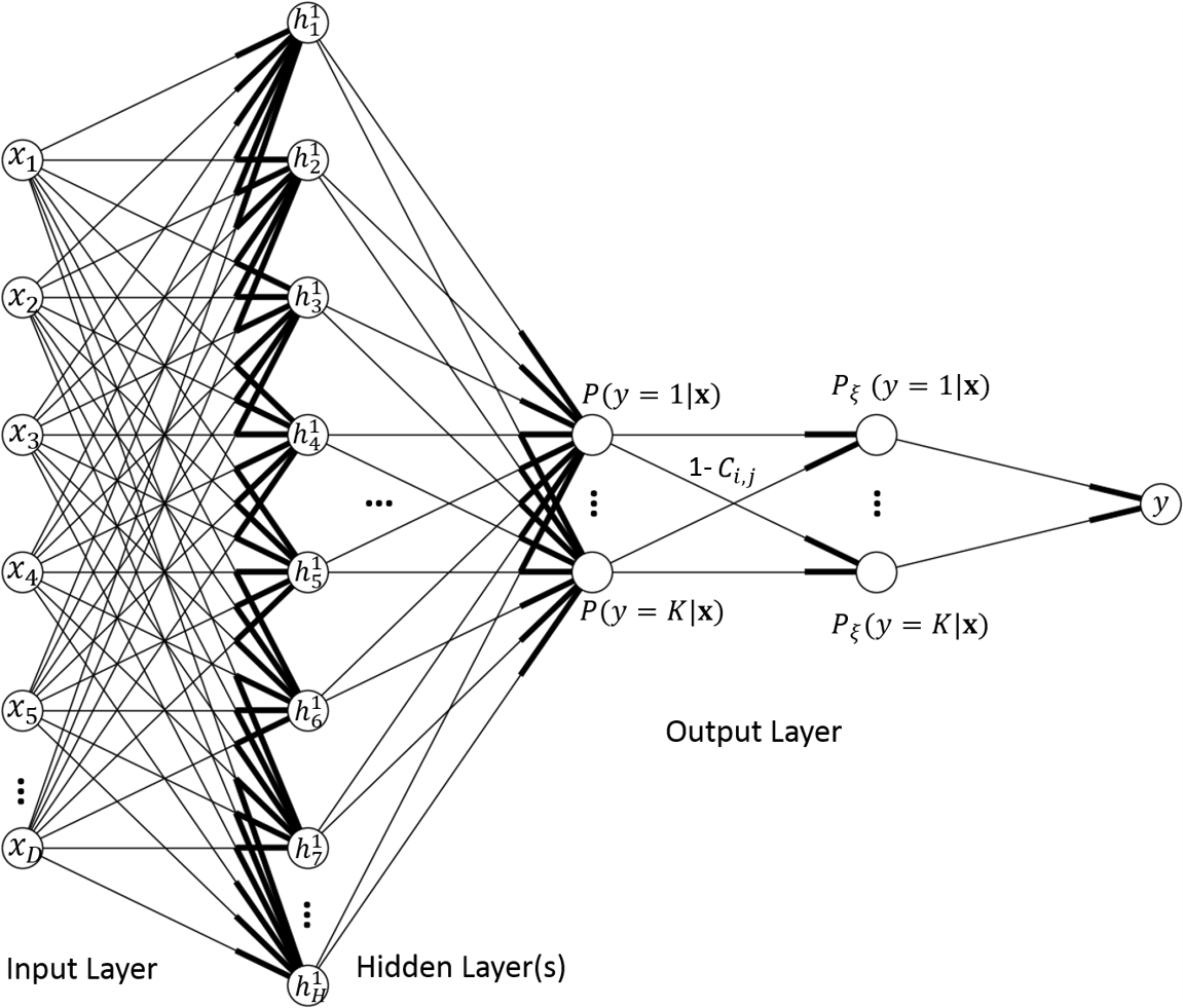
Figure 1: Schematic diagram of a cost-sensitive deep belief network (CSDBN) with misclassification costs for different classes in the output layer.

Suppose a dataset $S=\{\{\mathbf{x}_{1},y_{1}\},\{\mathbf{x}_{2},y_{2}\},\cdots,\{\mathbf{x}_{N},y_{N}\}\}$ contains a total number of $N$ data sample pairs $\{\mathbf{x}_{n},y_{n}\}$, where $\mathbf{x}_{n}$ is the $n$th data sample, $y_{n}$ is the corresponding $n$th target label. Assume a DBN consists of $H$ hidden layer and the parameters of each layer $i\in\{1,\cdots,H\}$ by $\theta_{i}=\{\mathbf{W}_{i},\mathbf{b}_{i}\}$. Given an input data sample $\mathbf{x}$ from the dataset, the DBN with $H$ hidden layer(s) presents a complex feature mapping function. After feature transformation, softmax layer serves as the output layer of DBN to perform classification predictions as parameterized by $\theta_{s}=\{\mathbf{W}_{s},\mathbf{b}_{s}\}$. Suppose there are $K$ neurons in the softmax layer, where the $j$-th neuron is responsible for estimating the prediction probability of class $j$ given input of ${\color[rgb]{0,0,0}\mathbf{x}_{H}}$ which is the output of the previous layer and associated with weights $\mathbf{W}_{s}^{(j)}$ and bias $\mathbf{b}_{s}^{(j)}$：

$$P(y=j|\mathbf{x})=\frac{exp(\mathbf{b}_{s}^{(j)}+{\color[rgb]{0,0,0}\mathbf{x}_{H}}^{T}\mathbf{W}_{s}^{(j)})}{\sum_{k=1}^{K}exp(\mathbf{b}_{s}^{(k)}+{\color[rgb]{0,0,0}\mathbf{x}_{H}}^{T}\mathbf{W}_{s}^{(k)})},$$ (1)

where ${\color[rgb]{0,0,0}\mathbf{x}_{H}}$ is the output of the previous layer. Based on the probability estimation, the trained DBN classifier provides a prediction as

$$f(\mathbf{x})=\arg\max_{1\leq j\leq K}P(y=j|\mathbf{x}).$$ (2)

In practice, the parameters $\{\theta_{1},\theta_{2},\cdots,\theta_{H},\theta_{s}\}$ of DBN are massively optimized by statistic gradient descent with respect to the negative log-likelihood loss over the training set $S_{t}$.

III-B Cost-sensitive Deep Belief Network

The concept of cost-sensitive learning is to minimize the overall cost (e.g. Bayes conditional risk [55]) on the training data set.

Assume the total number of classes is $K$, given a sample data $\mathbf{x}$, $C_{i,j}\in[0,1]$ denotes the cost of misclassifying $x$ as class $j$ when $x$ actually belongs to class $i$. In addition, $C_{i,j}=0$, when $i=j$, which indicates the cost for correct classification is 0.

Given the misclassification costs $C_{i,j}$, a data sample should be classified into the class that has the minimum expected cost. Based on decision theory [56], the decision rule minimizing the expectation cost $\mathcal{R}(i|\mathbf{x})$ of classifying an input vector $\mathbf{x}$ into class $i$ can be expressed as:

$$\mathcal{R}(i|\mathbf{x})=\sum_{j=1,j\neq i}^{K}P(j|\mathbf{x})C_{i,j}~{},$$ (3)

where $P(j|\mathbf{x})$ is the posterior probability estimation of classifying a data sample into class $j$. Given the prior probability $P(\mathbf{x}_{n})$, the general decision rule indicates which action to take for each data sample $\mathbf{x}_{n}$, thus the overall risk $\mathcal{R}$ is

$$\mathcal{R}=\sum_{n=1}^{N}\sum_{i=1}^{K}\mathcal{R}(i|\mathbf{x}_{n})P(\mathbf{x}_{n})$$ (4)

According to the Bayes decision theory, an ideal classifier will give a decision by computing the expectation risk of classifying an input to each class and predicts the label that reaches the minimum overall expectation risk. Misclassification costs represent penalties for classification errors. In cost-sensitive learning, all misclassification costs are essentially non-negative.

Mathematically, the probability that a sample data $\mathbf{x}\in S$ belongs to a class $j$, a value of a stochastic variable $y$, can be expressed as :

$$\begin{array}[]{rcl}P(y=j|\mathbf{x})&=&softmax_{j}(\mathbf{b}+\mathbf{W}\mathbf{x})\\ &=&\frac{exp({\mathbf{b}_{j}+\mathbf{W}_{j}x})}{\sum_{i}exp({\mathbf{b}_{i}+\mathbf{W}_{i}x})},\end{array}$$ (5)

The misclassification threshold values are introduced to turn posterior probabilities into class labels such that the misclassification costs are minimized. Implementing the misclassification threshold value $1-C_{i,j}$ on the obtained posterior probability $P(y=j|\mathbf{x})$, one can obtain the new probability $P_{\xi}$:

$$P_{\xi}(y=j|\mathbf{x})={\color[rgb]{0,0,0}P(y=j|\mathbf{x})}\cdot(1-C_{i,j}).$$ (6)

Generally, the misclassification threshold values for minority classes are larger than those of majority classes. The hypothesized prediction $f(\mathbf{x})$ of the sample $\mathbf{x}$ is the member of the maximum probability among classes, can be obtained by using the following equation:

$$F(\mathbf{x})=arg\max_{j}P_{\xi}(y=j|\mathbf{x}).$$ (7)

The proposed cost-sensitive learning method only concerns the output layer of a DBN. In this paper, we follow the same pre-training and fine-tuning procedures as in [24].

For imbalanced classification problems, the prior probability distribution of different classes is essentially imbalanced or non-uniform. To reflect class imbalance, there is a need to introduce the misclassification cost at the output layer to reflect the imbalanced class distributions. In addition, traditional training algorithms generally assume uniform class distribution with equal misclassification costs, i.e. $\forall i,j\in[1,2,\cdots,K]$, if $i=j,C_{i,j}=0$, if $i\neq j,C_{i,j}=1$, 　which is not true in many real-world applications.

In many real-world applications, the misclassification costs are essentially unknown and they vary across various classes. The current studies [55] usually attempt to determine misclassification costs by trial and error which generally does not lead to an optimal solution. Some studies [39] have devised mechanisms to update misclassification costs based on the number of samples in different classes. However, such methods may not be suitable for the cases where the classes are important but rare, such as some rare fatal diseases. To avoid hand tuning of misclassification costs, adaptive differential evolution algorithm [30] is implemented in this paper. Adaptive differential evolution algorithm is a simple effective and efficient evolutionary algorithm which could obtain optimal solution by evolving and updating a population of individuals during several generations. It attempts to adaptively self-update the control parameters without the need of prior knowledge.

IV Evolutionary Cost-Sensitive Deep Belief Network (ECS-DBN)

As discussed in Section II-B, evolutionary algorithm (EA) is a widely used optimization algorithm which is motivated by the biological evolution process. The EA algorithm can be designed to optimize the misclassification costs that are unknown in practice. In this paper, we propose an Evolutionary Cost-Sensitive Deep Belief Network (ECS-DBN) by incorporating cost-sensitive function directly into its classification paradigm with the misclassification costs being optimized through adaptive differential evolution [30, 57]. The main idea of this cost-sensitive learning technique is to assign class-dependent costs. Fig. 1 shows the schematic diagram of a cost-sensitive deep belief network.

The procedure of training the proposed ECS-DBN can be summarized in Table I. Firstly, a population of misclassification costs are randomly initialized. We then train a DBN with the training dataset. After applying misclassification costs on the outputs of the DBN, we evaluate the training error based on the performance of the corresponding cost-sensitive hypothesized prediction. According to the evaluation performance on training dataset, proper misclassification costs are selected to generate the population of next generation. In the next generation, mutation and crossover operators are employed to evolve a new population of misclassification costs. Adaptive differential evolution (DE) algorithm will proceed to next generation and continuously iterate between mutation and selection to reach the maximum number of generations. Eventually, the best found misclassification costs are obtained and applied to the output layer of DBN to form ECS-DBN as shown in Fig. 1. At run-time, we test the resulting ECS-DBN with test dataset to report the performance. The practical steps of ECS-DBN is summarized in Algorithm 1, and discussed next.

TABLE I: The training process of an Evolutionary Cost-Sensitive Deep Belief Network (ECS-DBN).

Pre-Training Phase:
1. Let $S_{t}$ be the training set.
2. Pre-train DBN using greedy layer-wise training algorithm with $S_{t}$.
Fine-Tuning Phase:
1. Randomly initialize a population of misclassification costs.
2. Generate a new population of misclassification costs via mutation and crossover based on differential operator.
3. Multiply the corresponding misclassification costs on training output and evaluate the error on training data.
4. According to evaluation performance, select appropriate misclassification costs and discard inappropriate ones in order to evolve next generation.
5. Continuously iterate between mutation and selection to reach the maximum number of generations.

Algorithm 1 Procedure of ECS-DBN

0:    $\mathbf{X}$: Imbalanced data samples$Y$: Class labels$N$: Population size$G$: Maximum number of generations (i.e. stopping criterion)$F$: Mutation factor$Cr$: Crossover probability$D$: Dimension of solution space$range=(\mathbf{c}_{min},\mathbf{c}_{max})$: Range of values for chromosome.Set $\mu_{Cr}=0.5,\mu_{F}=0.5,A=\emptyset,\beta=0.5.$

  Step 1) Initialization: Generate an initial population $\{\mathbf{c}_{0}^{1},\dots,\mathbf{c}_{0}^{N}\}$ via uniformly random sampling in solution space. The initial value of $i$th individual is generated as $\mathbf{c}_{0}^{i}=\mathbf{c}_{min}+rand(0,1)\cdot(\mathbf{c}_{max}-\mathbf{c}_{min})$. And evaluate each candidate solution $\mathbf{c}_{0}^{i}$ ($i=1,\cdots,N$) in the initial population via its corresponding trained $DBN(\mathbf{x}\in S_{t},y|\mathbf{c})$ to obtain a vector representing the fitness functions $F(\mathbf{c}_{0}^{i})$ which is G-mean of training dataset in this paper.

  Step 2) Evolution:

  for $g=1,\cdots,G$ do

     Set the set of all successful mutation factor $F_{i}$ at each generation $S_{F}=\emptyset;$

     Set the set of all successful crossover probabilities $Cr_{i}$ at each generation $S_{Cr}=\emptyset;$

     for $i=1,\cdots,N_{p}$ do

        Generate $Cr_{i}=randn(\mu_{Cr},0.1),F_{i}=randc_{i}(\mu_{F},0.1)$.

        Step 2.1) Mutation: Randomly select two indices $j$ and $k$ from population, then generate a new candidate solution $\mathbf{c}_{g}^{i^{\prime}}$ from $\mathbf{c}_{g}^{i}$, $\mathbf{c}_{g}^{j}$ and $\mathbf{c}_{g}^{k}$ by $\mathbf{c}_{g}^{i^{\prime}}$=$\mathbf{c}_{g}^{i}+F_{i}\cdot(\mathbf{c}_{g}^{j}-\mathbf{c}_{g}^{k})$, which is a DE operator.Generate $i_{rand}=randint(1,D)$

        Step 2.2) Crossover:

        if $i=i_{rand}$ or $rand(0,1)<Cr_{i}$ then

           $\mathbf{u}_{g}^{i}=\mathbf{c}_{g}^{i^{\prime}}$

        else

           $\mathbf{u}_{g}^{i}=\mathbf{c}_{g}^{i}$

        end if

        Step 2.3) Selection:

        if $F(\mathbf{c}_{g}^{i})\geq F(\mathbf{u}_{g}^{i})$ then

           $\mathbf{c}_{g+1}^{i}=\mathbf{c}_{g}^{i}$

        else

           $\mathbf{c}_{g+1}^{i}=\mathbf{u}_{g}^{i},\mathbf{c}_{g}^{i}\rightarrow A,Cr_{i}\rightarrow S_{Cr},F_{i}\rightarrow S_{F}$

        end if

        Randomly remove solutions from A so that $|A|\leq N$

        Step 2.4) Parameter Adaptation:

        $\mu_{Cr}=(1-\beta)\cdot\mu_{Cr}+\beta\cdot mean(S_{CR})$

        $\mu_{F}=(1-\beta)\cdot\mu_{F}+\beta\cdot mean(S_{F})$

     end for

  end for

  Step 3) ECS-DBN Creation: Generate an ECS-DBN with the best individual $\mathbf{c}_{best}$ obtained from the training dataset $S_{t}$ as the misclassification cost.

  Step 4) Run-time Evaluation: Evaluate ECS-DBN on test dataset $S_{test}$.

IV-A Chromosome Encoding

Chromosome encoding is an important step in evolutionary algorithms which aims at effectively representing important variables for better performance. In many real-world applications, misclassification costs in cost-sensitive deep belief network are usually unknown. In order to obtain appropriate costs, in our proposed approach each chromosome represents misclassification costs for different classes, and the final evolved best chromosome is chosen as the misclassification costs for ECS-DBN. The chromosome encoding here directly encodes the misclassification costs as values in the chromosome with numerical type and value range of $[0,1]$. Fig. 2 illustrates of chromosome encoding and evolution process in ECS-DBN.

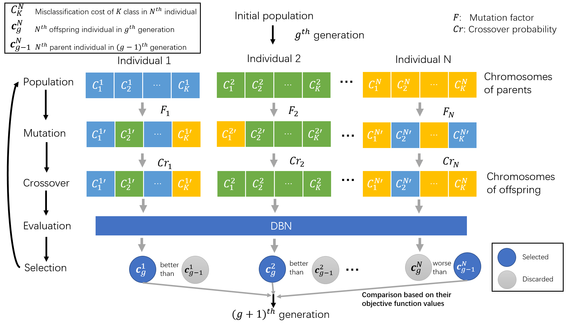
Figure 2: Illustration of chromosome encoding and evolution process in ECS-DBN. The chromosome is encoded with the misclassification costs of different classes in numerical type. The evolution process mainly includes mutation, crossover, evaluation and selection. The population is iteratively evolved via evolution process in each generation.

IV-B Population Initialization

The initial population is obtained via uniformly random sampling in feasible solution space for each variable within the specified range of the corresponding variable. The population is to hold possible misclassification costs and forms the unit of evolution. The evolution of the misclassification costs is an iterative process with the population in each iteration called a generation.

IV-C Adaptive DE Operators

After initialization, adaptive differential evolution evolves the population with a sequence of three evolutionary operations, i.e. mutation, crossover, and selection, generation by generation. Mutation is carried out with DE mutation strategy to create mutation individuals based on the current parent population as shown in Step 2.1 of Algorithm 1. After mutation, a binomial crossover operation is utilized to generate the final offspring as shown in Step 2.2 of Algorithm 1. In adaptive DE, each individual has its associated crossover probability instead of a fixed value. The selection operation selects the best one from the parent individuals and offspring individuals according to their corresponding fitness values as shown in Step 2.3 of Algorithm 1. Parameter adaptation is conducted at each generation. In this way, the control parameters are automatically updated to appropriate values without the need of prior parameter setting knowledge in DE. The crossover probability of each individual is generated independently based on a normal distribution with mean $\mu_{Cr}$ and standard deviation 0.1. Similarly, the mutation factor of each individual is generated independently based on a Cauchy distribution with location parameter $\mu_{F}$ and scale parameter 0.1. Both the mean $\mu_{Cr}$ and the location parameter $\mu_{F}$ are updated at the end of each generation as shown in Step 2.4 of Algorithm 1.

IV-D Fitness Evaluation

Fitness evaluation allows us to choose the appropriate misclassification costs. In the proposed method, each individual chromosome is introduced into individual DBN as misclassification costs. We generate suitable misclassification costs for DBN using the training set. G-mean of training set is chosen as the objective function for the optimization.

IV-E Termination Condition

Evolutionary algorithms are designed to evolve the population generation by generation and maintain the convergence as well as diversity characteristics within the population. A maximum number of generations is set to be a termination condition of the algorithm. In this implementation, we consider the solutions converged when the best fitness value remains unchanged over the past 30 generations [17]. The algorithm terminates either when it reaches the maximum number of generations or when it meets the convergence condition.

IV-F ECS-DBN Creation

Eventually, the optimization process ends with the best individual which is used as misclassification costs to form an ECS-DBN. The best individual is obtained from the last generation.

V Evaluation On Benchmark Datasets

In this section, the proposed ECS-DBN approach is evaluated on 58 popular KEEL benchmark datasets.

V-A Nomenclature

ADASYN, SMOTE and its various resampling methods are applied with DBN to generate synthetic minority data on the imbalanced datasets. The nomenclature convention used in labeling the imbalance learning methods are as follows: the prefix letters “ADASYN”, “SMOTE”, “SMOTE-SVM”, “SMOTE-borderline1”, and “SMOTE-borderline2” respectively, represent the adaptive synthetic sampling approach [13], Synthetic Minority Over-sampling Technique [12], Support Vectors SMOTE [58], and Borderline SMOTE of types 1 and 2 [14]. The suffix “-DBN” represents deep belief network.

V-B Benchmark Datasets

In this paper, benchmark datasets are selected from KEEL (Knowledge Extraction based on Evolutionary Learning) dataset repository [59]. The details specification of 58 binary-class imbalanced datasets are shown in Table II. All datasets are downloaded from KEEL website. They are known to have a high imbalance ratio between the majority and minority classes.

The imbalance ratio (IR) is the number of data samples in majority class divided by that in minority class which is described by (8).

$$\scriptsize IR=\frac{\#~{}majority}{\#~{}minority}$$ (8)

TABLE II: A summary of the KEEL binary-class imbalanced benchmark datasets. The details of each dataset includes its imbalance ratio, number of attributes, number of training data and number of test data. A total of 58 datasets used in this paper are listed below.

Datasets	Imbalance Ratio(IR)	Attributes	TrainData	TestData
abalone9-18	16.40	8	585	146
cleveland-0-vs-4	12.62	13	142	35
ecoli-0-1-3-7-vs-2-6	39.14	7	225	56
ecoli-0-1-4-6-vs-5	13.00	6	224	56
ecoli-0-1-4-7-vs-2-3-5-6	10.59	7	269	67
ecoli-0-1-4-7-vs-5-6	12.28	6	266	66
ecoli-0-1-vs-2-3-5	9.17	7	195	49
ecoli-0-1-vs-5	11.00	6	192	48
ecoli-0-2-3-4-vs-5	9.10	7	162	40
ecoli-0-2-6-7-vs-3-5	9.18	7	179	45
ecoli-0-3-4-6-vs-5	9.25	7	164	41
ecoli-0-3-4-7-vs-5-6	9.28	7	206	51
ecoli-0-3-4-vs-5	9.00	7	160	40
ecoli-0-4-6-vs-5	9.15	6	162	41
ecoli-0-6-7-vs-3-5	9.09	7	178	44
ecoli-0-6-7-vs-5	10.00	6	176	44
ecoli3	8.6	7	269	67
glass-0-1-2-3-vs-4-5-6	3.2	9	171	43
glass-0-1-4-6-vs-2	11.06	9	164	41
glass-0-1-5-vs-2	9.12	9	138	34
glass-0-1-6-vs-2	10.29	9	153	39
glass-0-1-6-vs-5	19.44	9	147	37
glass-0-4-vs-5	9.22	9	74	18
glass-0-6-vs-5	11.00	9	86	22
glass0	2.06	9	171	43
glass1	1.82	9	171	43
glass2	11.59	9	171	43
glass4	15.47	9	171	43
glass5	22.78	9	171	43
glass6	6.38	9	171	43
haberman	2.78	3	245	61
iris0	2	4	120	30
led7digit-0-2-4-5-6-7 -8-9-vs-1	10.97	7	354	89
new-thyroid1	5.14	5	172	43
newthyroid2	5.14	5	172	43
page-blocks-1-3-vs-4	15.86	10	378	94
page-blocks0	8.79	10	4378	1094
pima	1.87	8	614	154
segment0	6.02	19	1846	462
shuttle-c0-vs-c4	13.87	9	1463	366
shuttle-c2-vs-c4	20.50	9	103	26
vehicle0	3.25	18	677	169
vowel0	9.98	13	790	198
wisconsin	1.86	9	546	137
yeast-0-2-5-6-vs-3-7-8-9	9.14	8	803	201
yeast-0-2-5-7-9-vs-3-6-8	9.14	8	803	201
yeast-0-3-5-9-vs-7-8	9.12	8	405	101
yeast-0-5-6-7-9-vs-4	9.35	8	422	106
yeast-1-2-8-9-vs-7	30.57	8	757	188
yeast-1-4-5-8-vs-7	22.1	8	554	139
yeast-1-vs-7	14.30	7	367	92
yeast-2-vs-4	9.08	8	411	103
yeast-2-vs-8	23.10	8	385	97
yeast1	2.46	8	1187	297
yeast3	8.1	8	1187	297
yeast4	28.10	8	1187	297
yeast5	32.73	8	1187	297
yeast6	41.40	8	1187	297

V-C Implementation Details

The learning rates of both pre-training and fine-tuning are 0.01. The number of pre-training and fine-tuning iterations are 100 and 300 respectively. The range of hidden neuron number is $[5,50]$. The hidden neuron number of the networks are randomly selected from the range of hidden neuron number. Generally speaking, there are two key parameters that affect DE process namely mutation factor $F$ and crossover probability $Cr$. A larger $F$ enables DE of better exploration ability. A smaller $F$ allows DE to have better exploitation ability. DE with better exploitation ability leads to better convergence. DE with better exploration ability avoids local optima better, but it may result in slower convergence. Crossover probability affects the diversity of populations. A larger $Cr$ enables DE of better exploitation ability while a smaller $Cr$ enables DE of better exploration ability. We set the parameters empirically [30] to ensure that DE generally converges. All the codes of resampling methods for comparison in this paper are from [60] in Python and their corresponding parameters are set as default. All the simulation results are obtained with 5-fold cross validation over 10 trials. All of the simulations are done on an Intel Core i5 3.20GHz machine with 16 GB RAM and NVIDIA GeForce GTX 980.

V-D Evaluation Metrics

As in [32, 17, 13, 12, 14, 44, 58], accuracy, G-mean, F1-score, recall, precision are the most commonly used evaluation metrics. Considering an imbalance binary-class classification problem, let TP, FP, FN, TN represent true positive, false positive, false negative and true negative, respectively. To evaluate the performance of a classifier, it is common to use the overall accuracy that is formulated in (9).

$$Accuracy=\frac{TP+TN}{TP+TN+FP+FN}$$ (9)

In this section, both accuracy and G-mean are used. We use G-mean (10) because it evaluates the degree of inductive bias which considers both positive and negative accuracy. The higher G-mean values represent the classifier could achieve better performance on both minority and majority classes. G-mean is less sensitive to data distributions that is given as follows,

$$G\text{-}mean=\sqrt{\frac{TP}{TP+FN}\times\frac{TN}{TN+FP}}$$ (10)

V-E Results of ECS-DBN

In this section, we investigate the performance of DBN in different settings that include ECS-DBN, DBN, ADASYN-DBN, SMOTE-DBN, SMOTE-borderline1-DBN, SMOTE-borderline2-DBN and SMOTE-SVM-DBN. We report the results over a total of runs on 58 KEEL benchmark datasets in terms of test accuracy and test G-mean, respectively. A detailed summary can be found at Tables AI and AII in Annex, with the best results being highlighted in boldface. To visualize, Fig. 3 illustrates the overall performances of the 7 variations of DBN algorithms on 58 benchmark datasets. It is clear that ECS-DBN stands out from the rest.

From the simulation results, the proposed ECS-DBN exhibits superior overall performance, especially in terms of G-mean. From Table AII, we observe that ECS-DBN excels in 34 out of 58 benchmark datasets in terms of accuracy. As there are many more samples in majority class than minority class, a classifier can bias to the majority class yet achieve a high accuracy. We also report results in G-mean, that G-mean takes both performance of majority class and minority class into account. If some methods give a highly biased performance, their G-mean values will be close to 0. It is worth noting that ECS-DBN outperforms on 52 out of 58 benchmark datasets in terms of G-mean as shown in Table AII. We may attribute this to the fact that ECS-DBN has been optimized using evolutionary algorithm with maximized G-mean objective. Therefore, the proposed ECS-DBN can provide better performances on minority class as well as those on majority class.

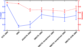
Figure 3: Comparison of the overall G-mean and accuracy across 7 algorithms, i.e. ECS-DBN, DBN, ADASYN-DBN, SMOTE-DBN, SMOTE-borderline1-DBN, SMOTE-borderline2-DBN and SMOTE-SVM-DBN, on 58 benchmark datasets. ECS-DBN has higher average values and lower variance for both G-mean and accuracy than other competing methods.

V-F Computational Time Analysis

The computing of ECS-DBN at run-time is closely related to the DBN network complexity. The larger and deeper network size of DBN, the more computing is required. Table III reports the average computational time of ECS-DBN with 5-fold cross validation over 10 trials on the overall 58 benchmark datasets. In order to make a fair and clear comparison between different imbalance learning methods, the average computational time at run-time testing is summarized in Table III. ECS-DBN shows a higher computational cost that is mainly due to the evolutionary algorithm. We note that the resampling methods are a little bit faster than ECS-DBN due to the small data size of KEEL benchmark datasets.

TABLE III: Comparison of the average computational time across 7 algorithms (i.e. ECS-DBN, DBN, ADASYN-DBN, SMOTE-DBN, SMOTE-borderline1-DBN, SMOTE-borderline2-DBN and SMOTE-SVM-DBN) with 5-fold cross validation on the overall 58 benchmark datasets over 10 trials.

Model Name	Average Computational Time(s)	Average Computational Time without DBN training time(s)
ECS-DBN	26.64 $\pm$ 1.50	18.23
ADASYN-DBN	22.97 $\pm$ 3.95	14.56
SMOTE-SVM-DBN	24.03 $\pm$ 2.33	15.62
SMOTE-borderline2-DBN	24.53 $\pm$ 2.14	16.12
SMOTE-borderline1-DBN	25.52 $\pm$ 2.59	17.11
SMOTE-DBN	25.81 $\pm$ 3.10	17.40
DBN	8.41 $\pm$ 1.28	-

V-G Statistical Tests for Evaluating Imbalance Learning

Statistical tests provide evidence to ascertain the claim that the ECS-DBN outperforms other competitive methods. It is noted that three common statistical tests  [16, 61, 62, 21, 63, 17], can serve our purpose. Wilcoxon paired signed-rank test is adopted for pairwise comparisons between algorithms. Alternatively for comparison between $\xi$ multiple algorithms, a Holm post-hoc test can be utilized to conduct a $1\times\xi$ posteriori tests between the control algorithm and the rest subgroups of algorithms. Average rank is also implemented for fair comparison.

V-G1 Wilcoxon Paired Signed-Rank Test

In order to substantiate whether the results of ECS-DBN and other kinds of imbalance learning methods differ in a statistically significant way, a nonparametric statistical test known as Wilcoxon paired signed-rank test is conducted at the 5% significance level. The Wilcoxon paired signed-rank test is employed separately between pairs of algorithms for each dataset. The entries which are significantly better than all the counterparts are marked with ${\dagger}$ in Tables AI and AII. The total number of win-lose-draw between the proposed method and its counterparts are then reckoned. The pairwise comparisons of the proposed ECS-DBN method against other kinds of methods in terms of accuracy and G-mean are shown in Tables AI and AII, respectively. In most cases, the proposed ECS-DBN method outperforms other state-of-the-art resampling methods, i.e. ADASYN, SMOTE, SMOTE-borderline1, SMOTE-borderline2 and SMOTE-SVM.

V-G2 Holm post-hoc Test

For multiple comparisons, different algorithms are compared using the Holm post-hoc test to detect statistical differences among them. The proposed ECS-DBN is chosen as the control algorithm for comparison. Then Holm post-hoc test is implemented on the results of the method for all datasets in terms of accuracy and G-mean as shown in Tables AI and AII, respectively. The $p$-values from Holm post-hoc test shown in Tables AI and AII indicates that the proposed ECS-DBN method statistically outperforms other methods with significant statistical differences based on the results of all 58 datasets. In Holm post-hoc test, ECS-DBN outperforms others.

V-G3 Average Rank

Average rank is the mean of the ranks of individual method on all the datasets. Average ranks provide a fair comparison in terms of accuracy and G-mean of different methods as shown in Tables AI and AII. Based on the average ranks in terms of both accuracy and G-mean on all datasets, the proposed ECS-DBN ranked first in the majority of the datasets. The results indicate that ECS-DBN outperforms other competing methods and excels especially in terms of G-mean. For a better illustration, the average rank of different algorithms in terms of G-mean and accuracy is shown in Fig. 4. It is apparent that ECS-DBN outranks others in terms of G-mean and accuracy.

In sum, the results show that ECS-DBN method significantly outperforms other competing methods. First of all, according to the Wilcoxon paired signed-rank test, ECS-DBN outperforms other methods in most cases. Secondly, the $p$-values from the Holm post-hoc test suggest that ECS-DBN achieves a statistically significant improvement over other competing methods. Thirdly, average ranks show that ECS-DBN is ranked first across most of the benchmark datasets. The fact that ECS-DBN outperforms DBN validates the need for cost-sensitive learning. Finally, the significant improvement of ECS-DBN over some other methods manifests the effectiveness of optimization.

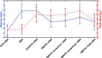
Figure 4: The average rank of 7 different algorithms, i.e. ECS-DBN, DBN, ADASYN-DBN, SMOTE-DBN, SMOTE-borderline1-DBN, SMOTE-borderline2-DBN and SMOTE-SVM-DBN, in terms of G-mean and accuracy on 58 KEEL benchmark datasets. ECS-DBN ranks first over other competing methods.

VI Evaluation On A Real-World Dataset

VI-A Overview of the Imbalanced Gun Drilling Dataset

We report the experiment results on gun drilling dataset collected from a UNISIG USK25-2000 gun drilling machine in Advanced Manufacturing Lab at the National University of Singapore, Singapore, in collaboration with SIMTech-NUS joint lab.

VI-B Experimental Setup

In the experiments, an Inconel 718 workpiece with the size of $1000mm*100mm*100mm$ is machined using gun drills. The tool diameter of gun drills is $8mm$. The detailed tool geometry of the tools are shown in Table VI. Four vibration sensors (Kistler Type 8762A50) are mounted on the workpiece in order to measure the vibration signals in three directions (i.e. $x$, $y$ and $z$) during the gun drilling process. The details about sensor types and measurements are shown in Table IV. The sensor signals are acquired via a NI cDAQ-9178 data acquisition device and logged on a laptop.

In data acquisition, 14 channels of raw signals belonging to three types are logged. The measured signals include force signal, torque signal, and 12 vibration signals (i.e. acquired by 4 accelerometers in $x,y,z$ directions). The tool wears have been measured using Keyence VHX-5000 digital microscope. In this paper, the maximum flank wear which is most widely used in literature [64, 5, 65, 66, 67, 6] has been used as the health indicator of the tool. In this dataset, it is found 3 out of 20 tools are broken, 6 out of 20 tools have chipping at final state and 11 out of 20 tools are worn after gun drilling operations.

TABLE IV: A summary of the 3 different types of sensors (i.e. accelerometer, dynamometer and microscope) used in the gun drilling experiments and the obtained measurements including vibration, force, torque and tool wear.

Sensor type	Vibration Sensor	Force Torque Sensor	Microscope
Description	Kistler 50g 3-axis accelerometer Type 8762A50	Dynamometer embedded in USK25-2000 machine	Keyence VHX-5000 Digital Microscope
# Sensors	4	1	-
# Channels per sensors	3	2	-
Total number of channels	12	2	-
Measurements	Vibration X,Y,Z	Thrust force, torque	Tool wear
Sampling frequency (Hz)	20,000	100	-

TABLE V: Detailed number of data samples and imbalance ratio of the imbalanced gun drilling dataset.

Number of Signal Channels	14
Total Number of Data Samples	19,712,414
Number of Training Samples	13,798,690
Number of Testing Samples	5,913,724
Imbalance Ratio	10

The machining operation is carried out with the detailed hole index, drill depth, tool geometry, tool diameter, feed rates, spindle speeds, machining times and tool final states are shown in Table VI. The drilling depth is 50 mm in $z$-axis direction. The tool wear is captured and measured by Keyence digital microscope. The tool wear is measured after each drill during gun drilling operations.

TABLE VI: Detailed real-world high aspect ratio deep hole gun drilling experimental conditions include tool diameter, spindle speed, feed rate and machining time for 20 drilling inserts with 6 different tool geometries.

Hole Index	Drill Depth (mm)	Tool Geometry	Tool Diameter (mm)	Spindle Speed (rpm)	Feed Rate ($\mu m$/rev)	Machining Time(s)
H1_01	50	1450mm_N4_R9	8.05	1200	20	125.00
H1_02	50		8.05	1200	20	125.00
H2_01	50	1450mm_N4_R1	8.05	800	20	187.50
H2_02	50	1450mm_N4_R1	8.05	800	20	187.50
H2_03	50	1650mm_N8_R1	8.02	1650	16	113.64
H3_01	50	1450mm_N8_R9	8.05	1650	16	113.64
H3_02	50		8.05	1650	16	113.64
H3_03	50		8.05	1650	16	113.64
H3_04	50	1450mm_N8_R9	8.05	1650	16	113.64
H3_05	50		8.05	1650	16	113.64
H3_06	50	1650mm_N8_R9	8.02	1650	16	113.64
H3_07	50		8.02	1650	16	113.64
H3_08	50	1650mm_N8_R9	8.02	1650	16	113.64
H3_09	50		8.02	1650	16	113.64
H3_10	50	1650mm_N8_R1	8.02	1650	16	113.64
H4_01	50	1219mm_N8_R9	8.08	1650	16	113.64
H4_02	50		8.08	1650	16	113.64
H4_03	50		8.08	1650	16	113.64
H5_01	50	1450mm_N8_R9	8.045	1650	16	113.64
H5_02	50	1450mm_N8_R9	8.045	1650	16	113.64

Table V lists the details of the imbalanced gun drilling dataset. The imbalanced gun drilling dataset is selected from the raw experimental data by discarding lousy noise data samples. The total number of data samples in the imbalanced gun drilling dataset is 19,712,414. The number of training data samples and test data samples are 13,798,690 and 5,913,724 respectively. The data has been labeled into healthy (i.e. maximum flank wear of the tool $<300\mu m$) and faulty (i.e. maximum flank wear of the tool $\geq 300\mu m$) two classes. The imbalance ratio (IR) of this dataset is 10. The data preprocessing and time window process are the same with [5].

TABLE VII: Comparing the performance of between Deep Belief Network (DBN) and Support Vector Machine (SVM), Multilayer Perceptron (MLP), K-Nearest Neighbor Classifier (KNN), Gradient Boosting (GB), Logistic Regression (LR), AdaBoost classifier, Lasso, and SGD different machine learning algorithms on gun drilling imbalanced dataset in terms of accuracy, G-Mean, AUC, precision, F1-score. DBN outperforms other competing methods in terms of all evaluation metrics.

Model Name	Accuracy	G-mean	AUC	Precision	F1-score
DBN	0.9954 $\pm$ 0.0006	0.9830 $\pm$ 0.0027	0.9831 $\pm$ 0.0027	0.9968 $\pm$ 0.0005	0.9975 $\pm$ 0.0003
SVM	0.9894 $\pm$ 0.0103†	0.8943 $\pm$ 0.3143	0.9443 $\pm$ 0.1562	0.9898 $\pm$ 0.0284	0.9944 $\pm$ 0.0148
MLP	0.9683 $\pm$ 0.0064	0.8492 $\pm$ 0.0350†	0.8601 $\pm$ 0.0296†	0.9733 $\pm$ 0.0056	0.9827 $\pm$ 0.0035
KNN	0.9733 $\pm$ 0.0026	0.8460 $\pm$ 0.0214†	0.8579 $\pm$ 0.0181†	0.9725 $\pm$ 0.0035	0.9855 $\pm$ 0.0014†
GB	0.9821 $\pm$ 0.0353	0.8088 $\pm$ 0.3910†	0.9025 $\pm$ 0.1947†	0.9822 $\pm$ 0.0354	0.9906 $\pm$ 0.0185†
LR	0.9412 $\pm$ 0.0096	0.5903 $\pm$ 0.1058†	0.6791 $\pm$ 0.0545†	0.9398 $\pm$ 0.0095	0.9687 $\pm$ 0.0049†
AdaBoost	0.9361 $\pm$ 0.0126	0.5362 $\pm$ 0.1246†	0.6510 $\pm$ 0.0719†	0.9349 $\pm$ 0.0127	0.9661 $\pm$ 0.0065
Lasso	0.9523 $\pm$ 0.0414	0.5065 $\pm$ 0.4817†	0.7401 $\pm$ 0.2303†	0.9524 $\pm$ 0.0416	0.9749 $\pm$ 0.0216†
SGD	0.9258 $\pm$ 0.0169†	0.3860 $\pm$ 0.2692†	0.6098 $\pm$ 0.0894†	0.9281 $\pm$ 0.0162	0.9606 $\pm$ 0.0095†

${\dagger}$ indicates that the difference between marked algorithm and the proposed algorithm is statistically significant using Wilcoxon rank sum test at the $5\%$ significance level.

TABLE VIII: Comparing the performance of ECS-DBN, CSDBN, SMOTE-SVM-DBN, ADASYN-DBN, SMOTE-borderline1-DBN, SMOTE-borderline2-DBN, SMOTE-DBN, DBN, weighted extreme learning machine (WELM) and ECO-ensemble on gun drilling imbalanced dataset in terms of accuracy, G-mean, AUC, precision, F1-score. ECS-DBN shows better performance in terms of G-mean, AUC and precision.

Model Name	Accuracy	G-mean	AUC	Precision	F1-score
ECS-DBN	0.9960 $\pm$ 0.0002	0.9946 $\pm$ 0.0011	0.9946 $\pm$ 0.0011	0.9996 $\pm$ 0.0002	0.9978 $\pm$ 0.0001
CSDBN	0.9957 $\pm$ 0.0012	0.9916 $\pm$ 0.0026	0.9916 $\pm$ 0.0025	0.9987 $\pm$ 0.0007	0.9977 $\pm$ 0.0006
SMOTE-SVM-DBN	0.9961 $\pm$ 0.0003	0.9858 $\pm$ 0.0011	0.9859 $\pm$ 0.0011	0.9974 $\pm$ 0.0002†	0.9978 $\pm$ 0.0002
ADASYN-DBN	0.9964 $\pm$ 0.0004	0.9857 $\pm$ 0.0016	0.9858 $\pm$ 0.0016†	0.9973 $\pm$ 0.0003	0.9980 $\pm$ 0.0002
SMOTE-borderline2-DBN	0.9962 $\pm$ 0.0001	0.9852 $\pm$ 0.0010†	0.9853 $\pm$ 0.0010	0.9972 $\pm$ 0.0002	0.9979 $\pm$ 0.0001
SMOTE-borderline1-DBN	0.9958 $\pm$ 0.0003	0.9837 $\pm$ 0.0021	0.9838 $\pm$ 0.0020	0.9969 $\pm$ 0.0004	0.9977 $\pm$ 0.0002
SMOTE-DBN	0.9959 $\pm$ 0.0001	0.9837 $\pm$ 0.0010†	0.9838 $\pm$ 0.0010	0.9969 $\pm$ 0.0002†	0.9978 $\pm$ 0.0001†
DBN	0.9954 $\pm$ 0.0006	0.9830 $\pm$ 0.0027	0.9831 $\pm$ 0.0027†	0.9968 $\pm$ 0.0005	0.9963 $\pm$ 0.0003†
WELM	0.7397 $\pm$ 0.0177†	0.7532 $\pm$ 0.0170†	0.7841 $\pm$ 0.0159†	0.6274 $\pm$ 0.0202†	0.7261 $\pm$ 0.0148†
ECO-ensemble	0.9895 $\pm$ 0.0014†	0.9713 $\pm$ 0.0133†	0.9694 $\pm$ 0.0185†	0.9836 $\pm$ 0.0105†	0.9925 $\pm$ 0.0042†

${\dagger}$ indicates that the difference between marked algorithm and the proposed algorithm is statistically significant using Wilcoxon rank sum test at the $5\%$ significance level.

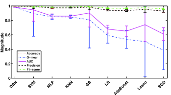
Figure 5: Illustration of the performance between different machine learning algorithms, i.e. DBN and SVM, MLP, KNN, GB, LR, AdaBoost, Lasso, and SGD, on gun drilling imbalanced dataset in terms of accuracy, G-Mean, AUC, precision, F1-score. DBN provides higher average values on all evaluation metrics than other methods.

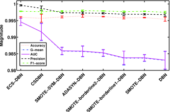
Figure 6: Illustration the performance of between different imbalance learning methods, i.e. ECS-DBN, CSDBN, SMOTE-SVM-DBN, ADASYN-DBN, SMOTE-borderline1-DBN, SMOTE-borderline2-DBN, SMOTE-DBN and baseline DBN, on gun drilling imbalanced dataset in terms of accuracy, G-Mean, AUC, precision, F1-score. ECS-DBN shows better performance than other resampling methods in terms of G-mean, AUC and precision.

The details of the gun drilling cycle are as follows.

1. Machine startup.

2. Feed internal coolant through coolant hole of gun drill.

3. Start to drill through the workpiece.

4. Finish drilling and pull the tool back.

5. Machine shutdown.

The internally-fed coolant will exhaust the heat generated during gun drilling process and give high accuracy and precision performance.

Figure 7: The procedure of gun drilling experiments includes 5 steps, namely start machine, feed coolant, start gun grilling in the workpiece, finish drilling & pull back the drill and finally shutdown the machine.

VI-C Evaluation Metrics

In this section, despite the evaluation metrics used in Section V-D, AUC, precision and F1-Score are introduced to evaluate the methods. The formulation of those metrics are listed below:

$$Precision=\frac{TP}{TP+FP}$$ (11)

$$Recall=\frac{TP}{TP+FN}$$ (12)

$$F1\textendash score=2\cdot\frac{precision\times recall}{precision+recall}$$ (13)

Precision (11) is a measure of a classifiers exactness. For this real-world application, exactness of classifier is an important indicator. F1-score (13) is a weighted average of precision and recall. The reason for choosing F1-score in this real-world application is that F1-score is used to evaluate the performance of the minority class (i.e. faulty) which is very important in this application. G-mean and F1-score incorporate both to express their tradeoff [32] and indicate the overall performance. AUC is used to evaluate the overall performance of the method on both classes. Recall is also known as the true positive rate, which signifies a measure of completeness.

VI-D Experiment Results

In this section, all the parameters of DBN and adaptive DE are the same with those in Section V. All conventional machine learning algorithms for comparison purpose in this paper are from [68] and their corresponding parameters are set as default. The resampling methods for comparison in this section are the same with Section V. Since there is only one real-world dataset, only Wilcoxon paired signed-rank test has been implemented in this section.

The simulation results of imbalanced gun drilling dataset with DBN, multi-layer neural network (MLP), support vector machine (SVM), K-nearest neighbors (KNN), linear classifier with stochastic gradient descent (SGD) training, logistic regression (LR), gradient boosting (GB), AdaBoost classifier, Lasso are shown in Table VII in terms of classification accuracy, G-means, Precision and F1-score on test data. For better illustration, Fig. 5 presents the errorbar plot of the performance between different algorithms evaluated with different metrics. All the simulation results include the average performances and the corresponding standard deviation values. The simulation results are obtained on test data. Based on the simulation results, it is obvious that DBN outperforms other 9 conventional machine learning algorithms. This could contribute to the strong feature learning ability of DBN. Therefore, with its automatically hierarchical feature learning ability, DBN is chosen as the base classifier for this real-world application.

Table VIII presents the comparison between ECS-DBN, CSDBN, weighted extreme learning machine (WELM), ECO-ensemble and various resampling methods including ADASYN, SMOTE, SMOTE-borderline1, SMOTE-borderline2 and SMOTE-SVM in terms of accuracy, G-mean, Precision, F1-score. For clear illustration, Fig. 6 shows the errorbar plot comparison of the performance between ECS-DBN and different resampling methods with different evaluation metrics. WELM [20] is a state-of-the-art cost-sensitive extreme learning machine. ECO-ensemble [17] incorporates synthetic data generation within an ensemble framework optimized by EA simultaneously. The experiment results show that ECS-DBN outperforms WELM and ECO-ensemble. By comparing with other resampling methods, ECS-DBN outperforms on G-mean and precision metrics. Especially on G-mean, ECS-DBN generates a significant performance improvement over the others.

As an example, we illustrate the G-mean and precision between ECS-DBN and the grid search of misclassification costs of DBN in Fig. 8. It is clear that the proposed ECS-DBN benefits from the well optimized misclassification costs to achieve better performance. In terms of accuracy and F1-score, ECS-DBN can also provide comparable performance. The performance improvement of ECS-DBN over DBN and CSDBN with randomly generated cost values on many performance metrics further illustrates the need for cost-sensitive learning and the effectiveness of optimization. Therefore, ECS-DBN could generate comparable performance not only on benchmark dataset but also on real-world application.

We further examine the effect of the proposed ECS-DBN over majority verse minority classes. Fig. 9 shows that ECS-DBN benefits from more suitable misclassification costs and improves the accuracy of minority class. Fig. 8 and Fig. 9 validate the ability of ECS-DBN of finding suitable misclassification costs via evolutionary algorithm that improves the accuracy of minority class, thus the overall performance. How ECS-DBN may impact on the majority class depends on the way we define the objective functions. While ECS-DBN improves the overall performance, it also provides a mechanism to trade off the performance between the majority class and the minority class.

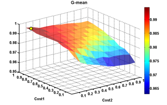
(a) G-mean

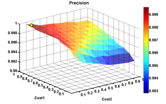
(b) Precision

Figure 8: Illustration of the comparison between the performance of the proposed ECS-DBN and grid search of misclassification costs on DBN in terms of G-mean and Precision. Note that the solid yellow circle represents the performance of ECS-DBN. This example indicates the proposed ECS-DBN can obtain better performance by finding suitable misclassification costs.

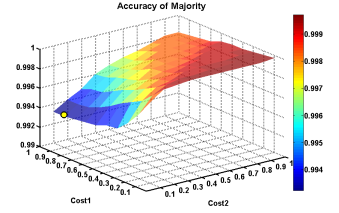
(a) Accuracy of majority class

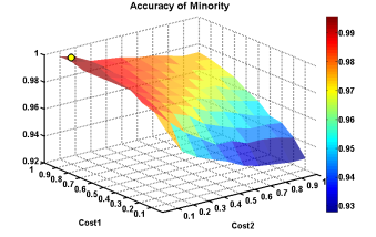
(b) Accuracy of minority class

Figure 9: Illustration of the comparison between the accuracy of majority class and minority class respectively with the proposed ECS-DBN and grid search of misclassification costs on DBN. Note that the solid yellow circle denotes the performance of ECS-DBN.

VI-E Computational Cost

Average computational time of ECS-DBN, DBN, ADASYN-DBN, SMOTE-DBN, SMOTE-borderline1-DBN, SMOTE-borderline2-DBN and SMOTE-SVM-DBN on the gun drilling imbalanced dataset are presented in Table IX. It is obvious that ECS-DBN consumes less average computational time than other competing methods. In comparison with the KEEL benchmark datasets, the gun drilling imbalanced dataset has a much larger size of data samples which increases the computational complexity for resampling methods. Hence, the proposed ECS-DBN is more efficient than some resampling methods to large dataset. If we compare the computational time required between the evolutionary algorithm to estimate the misclassification cost, and the DBN training, the former is very small and negligible. In short, the proposed ECS-DBN approach is both efficient and effective.

TABLE IX: Comparison of the average computational time across 7 algorithms (i.e. ECS-DBN, DBN, ADASYN-DBN, SMOTE-DBN, SMOTE-borderline1-DBN, SMOTE-borderline2-DBN and SMOTE-SVM-DBN) with 5-fold cross validation on the gun drilling imbalanced dataset over 10 trials.

Model Name	Average Computational Time(s)	Average Computational Time without DBN training time(s)
ECS-DBN	9977.39 $\pm$ 148.55	1280.28
ADASYN-DBN	12697.79 $\pm$ 1287.39	4000.68
SMOTE-DBN	13992.46 $\pm$ 1772.37	5295.35
SMOTE-borderline1-DBN	14031.35 $\pm$ 1135.55	5334.24
SMOTE-borderline2-DBN	14310.19 $\pm$ 764.11	5613.08
SMOTE-SVM-DBN	20942.94 $\pm$ 6609.65	12245.83
DBN	8697.11 $\pm$ 8308.22	-

VII Conclusion

In this paper, an evolutionary cost-sensitive deep belief network (ECS-DBN) is proposed for imbalanced classification problem. We have shown that ECS-DBN significantly outperforms other competing techniques on 58 benchmark datasets and a real-world dataset. The proposed ECS-DBN improves DBN by applying cost-sensitive learning strategy. To tackle with unknown misclassification costs in practice, adaptive differential evolution algorithm has been utilized to find the misclassification costs. Since many real-world data are naturally imbalanced, therefore, the misclassification costs of different classes are usually unknown, ECS-DBN offers an effective solution. ECS-DBN is also computationally more efficient than some popular resampling methods on large scale datasets. It can also be easily implemented on multi-class scenarios. In this paper, we only incorporate the cost-sensitive learning technique on algorithmic level. However, the imbalanced distribution in feature space may also impact the performance of learning models. In the future, we consider that cost-sensitive methods could also be applied to high dimensional data and dynamic data. Furthermore, online learning usually suffers from concept drift with different imbalance ratio over time. ECS-DBN can be further extended for online imbalanced classification problems with some online learning strategies. The proposed approach can also be applied to other deep learning models such as convolutional neural network, etc.

Chong Zhang received the B.Eng. degree in Engineering from Harbin Institute of Technology, China, and the M.Sc. degree from National University of Singapore in 2011 and 2012, respectively. She is currently a Ph.D. student as well as a research engineer in Department of Electrical and Computer Engineering at National University of Singapore. Her research interests include computational intelligence, machine learning/deep learning, data science and their applications in big data analytics, diagnostics, prognostics, health condition monitoring, voice conversion, etc.

Kay Chen Tan (SM’08–F’14) is a full Professor with the Department of Computer Science, City University of Hong Kong. He is the Editor-in-Chief of IEEE Transactions on Evolutionary Computation, was the EiC of IEEE Computational Intelligence Magazine (2010-2013), and currently serves on the Editorial Board member of 20+ journals. He is an elected member of IEEE CIS AdCom (2017-2019). He has published 200+ refereed articles and 6 books. He is a Fellow of IEEE.

Haizhou Li (M’91–SM’01–F’14) received the B.Sc., M.Sc., and Ph.D degree in electrical and electronic engineering from South China University of Technology, Guangzhou, China in 1984, 1987, and 1990 respectively. Dr Li is currently a Professor at the Department of Electrical and Computer Engineering, National University of Singapore (NUS). He is also a Conjoint Professor at the University of New South Wales, Australia. His research interests include automatic speech recognition, speaker/language recognition, and natural language processing. Prior to joining NUS, he taught in the University of Hong Kong (1988-1990) and South China University of Technology (1990-1994). He was a Visiting Professor at CRIN in France (1994-1995), Research Manager at the Apple-ISS Research Centre (1996-1998), Research Director in Lernout & Hauspie Asia Pacific (1999-2001), Vice President in InfoTalk Corp. Ltd. (2001-2003), and the Principal Scientist and Department Head of Human Language Technology in the Institute for Infocomm Research, Singapore (2003-2016). Dr Li is currently the Editor-in-Chief of IEEE/ACM Transactions on Audio, Speech and Language Processing (2015-2018), a Member of the Editorial Board of Computer Speech and Language (2012-2018). He was an elected Member of IEEE Speech and Language Processing Technical Committee (2013-2015), the President of the International Speech Communication Association (2015-2017), the President of Asia Pacific Signal and Information Processing Association (2015-2016), and the President of Asian Federation of Natural Language Processing (2017-2018). He was the General Chair of ACL 2012 and INTERSPEECH 2014. Dr Li is a Fellow of the IEEE. He was a recipient of the National Infocomm Award 2002 and the President’s Technology Award 2013 in Singapore. He was named one of the two Nokia Visiting Professors in 2009 by the Nokia Foundation.

Geok Soon Hong received the B.Eng. degree in Control Engineering in 1982 from University of Sheffield, UK. He was awarded a university scholarship to further his studies and obtained a Ph.D. degree in control engineering in 1987. The topic of his research was in stability and performance analysis for systems with multi-rate sampling problems. He is now an Associate Professor at the Department of Mechanical Engineering, National University of Singapore (NUS), Singapore. His research interests are in Control Theory, Multirate sampled data system, Neural network Applications and Industrial Automation, Modeling and control of Mechanical Systems, Tool Condition Monitoring, AI techniques in monitoring and Diagnostics.

Annex

TABLE AI: Summary of the test accuracy across 7 different algorithms, i.e. ECS-DBN, DBN and a group of resampling methods including ADASYN-DBN, SMOTE-DBN, SMOTE-borderline1-DBN, SMOTE-borderline2-DBN, SMOTE-SVM-DBN, on 58 KEEL benchmark datasets. ECS-DBN outperforms DBN and a group of resampling methods on 34 out of 58 benchmark datasets.

Datasets	ECS-DBN	DBN	Resampling Methods
			ADASYN-DBN	SMOTE-DBN	SMOTE -borderline1 -DBN	SMOTE-borderline2 -DBN	SMOTE-SVM -DBN
abalone9-18	0.9307$\pm$0.0048	0.9403$\pm$0.0045	0.7674$\pm$0.0061	0.6510$\pm$0.0457	0.7217$\pm$0.0754	0.7014$\pm$0.0954	0.7033$\pm$0.0177
cleveland-0_vs_4	0.9858$\pm$0.0115	0.9467$\pm$0.0115	0.6939$\pm$0.1419	0.7585$\pm$0.2254	0.8317$\pm$0.1145	0.7915$\pm$0.1242	0.8293$\pm$0.1698
ecoli-0-1-3-7_vs_2-6	0.9697$\pm$0.0001	0.9859$\pm$0.0052	0.9031$\pm$0.0966	0.8482$\pm$0.1337	0.8438$\pm$0.1397	0.7810$\pm$0.1407	0.9188$\pm$0.0744
ecoli-0-1-4-6_vs_5	0.9582$\pm$0.0001	0.9729$\pm$0.0146	0.7273$\pm$0.0000	0.8454$\pm$0.1201	0.6092$\pm$0.1756	0.7354$\pm$0.1552	0.8500$\pm$0.1328
ecoli-0-1-4-7_vs_2-3-5-6	0.9512$\pm$0.0005	0.9647$\pm$0.0000	0.6148$\pm$0.0518	0.7260$\pm$0.1890	0.8909$\pm$0.1020	0.7253$\pm$0.1524	0.7188$\pm$0.2138
ecoli-0-1-4-7_vs_5-6	0.9622$\pm$0.0002	0.9560$\pm$0.0218	0.6661$\pm$0.1150	0.7773$\pm$0.1822	0.7929$\pm$0.1830	0.8714$\pm$0.0674	0.8019$\pm$0.1890
ecoli-0-1_vs_2-3-5	0.9750$\pm$0.0042	0.9689$\pm$0.0000	0.7143$\pm$0.0502	0.6491$\pm$0.1826	0.7209$\pm$0.1478	0.6209$\pm$0.1444	0.6782$\pm$0.2011
ecoli-0-1_vs_5	0.9498$\pm$0.0049	0.9686$\pm$0.0058	0.7200$\pm$0.0000	0.8318$\pm$0.1031	0.8091$\pm$0.1695	0.7236$\pm$0.1463	0.8900$\pm$0.1042
ecoli-0-2-3-4_vs_5	0.9730$\pm$0.0051†	0.9029$\pm$0.0101	0.6613$\pm$0.0000	0.7253$\pm$0.2016	0.5527$\pm$0.1755	0.5560$\pm$0.1098	0.7582$\pm$0.1888
ecoli-0-2-6-7_vs_3-5	0.9475$\pm$0.0067	0.9772$\pm$0.0186	0.6049$\pm$0.0000	0.5040$\pm$0.1659	0.3851$\pm$0.0189	0.3832$\pm$0.0219	0.5505$\pm$0.2114
ecoli-0-3-4-6_vs_5	0.9441$\pm$0.0009	0.9596$\pm$0.0284	0.6719$\pm$0.0000	0.6860$\pm$0.2410	0.6774$\pm$0.1987	0.4785$\pm$0.0913	0.6860$\pm$0.2461
ecoli-0-3-4-7_vs_5-6	0.9358$\pm$0.0079	0.9477$\pm$0.0212	0.6158$\pm$0.0832	0.6526$\pm$0.1581	0.7155$\pm$0.2012	0.6534$\pm$0.1423	0.7250$\pm$0.1821
ecoli-0-3-4_vs_5	0.9480$\pm$0.0094	0.9007$\pm$0.0079	0.6774$\pm$0.0000	0.7344$\pm$0.1932	0.7767$\pm$0.1818	0.5689$\pm$0.1526	0.8133$\pm$0.1103
ecoli-0-4-6_vs_5	0.9741$\pm$0.0253†	0.9431$\pm$0.0326	0.6984$\pm$0.0000	0.6641$\pm$0.1879	0.6391$\pm$0.1857	0.5174$\pm$0.1388	0.7391$\pm$0.1852
ecoli-0-6-7_vs_3-5	0.9564$\pm$0.0100	0.9696$\pm$0.0121	0.6000$\pm$0.0651	0.6300$\pm$0.2025	0.5010$\pm$0.1641	0.4720$\pm$0.1193	0.7270$\pm$0.1862
ecoli-0-6-7_vs_5	0.8664$\pm$0.0077	0.9636$\pm$0.0000	0.6184$\pm$0.0000	0.5980$\pm$0.1729	0.5470$\pm$0.1443	0.4980$\pm$0.1305	0.5730$\pm$0.1939
ecoli3	0.9567$\pm$0.0050†	0.8936$\pm$0.0082	0.5920$\pm$0.0000	0.7212$\pm$0.1748	0.7245$\pm$0.1734	0.7033$\pm$0.1344	0.8252$\pm$0.1220
glass-0-1-2-3_vs_4-5-6	0.9597$\pm$0.0074	0.9815$\pm$0.0136	0.5795$\pm$0.1187	0.7415$\pm$0.1704	0.5402$\pm$0.1153	0.4829$\pm$0.0427	0.7768$\pm$0.2115
glass-0-1-4-6_vs_2	0.9890$\pm$0.0038†	0.9038$\pm$0.0000	0.7286$\pm$0.0000	0.4915$\pm$0.0580	0.4872$\pm$0.0551	0.4777$\pm$0.0498	0.6667$\pm$0.0000
glass-0-1-5_vs_2	0.9356$\pm$0.0214†	0.8864$\pm$0.0000	0.6066$\pm$0.0000	0.5154$\pm$0.0426	0.5128$\pm$0.0472	0.4974$\pm$0.0132	0.7193$\pm$0.0000
glass-0-1-6_vs_2	0.6711$\pm$0.0002	0.8980$\pm$0.0000	0.6667$\pm$0.0000	0.4795$\pm$0.0407	0.5273$\pm$0.0398	0.5170$\pm$0.0497	0.6377$\pm$0.0000
glass-0-1-6_vs_5	0.6761$\pm$0.0110	0.9364$\pm$0.0000	0.5325$\pm$0.0551	0.6432$\pm$0.2084	0.6261$\pm$0.2060	0.7011$\pm$0.1824	0.7627$\pm$0.0000
glass-0-4_vs_5	0.9346$\pm$0.0001†	0.8763$\pm$0.0067	0.6000$\pm$0.0935	0.5524$\pm$0.1713	0.5286$\pm$0.1475	0.5000$\pm$0.0502	0.5738$\pm$0.2204
glass-0-6_vs_5	0.9636$\pm$0.0288†	0.8941$\pm$0.0329	0.6409$\pm$0.0144	0.5000$\pm$0.0422	0.5760$\pm$0.1632	0.5600$\pm$0.1323	0.6180$\pm$0.1153
glass0	0.9513$\pm$0.0175†	0.6664$\pm$0.0250	0.5231$\pm$0.0000	0.5542$\pm$0.0963	0.5347$\pm$0.0672	0.4681$\pm$0.0262	0.5597$\pm$0.0980
glass1	0.7196$\pm$0.0282†	0.6487$\pm$0.0527	0.4444$\pm$0.0000	0.5145$\pm$0.0765	0.4986$\pm$0.0730	0.5101$\pm$0.0658	0.5246$\pm$0.0482
glass2	0.9721$\pm$0.0001†	0.9091$\pm$0.0000	0.6216$\pm$0.0000	0.4485$\pm$0.0630	0.4768$\pm$0.0916	0.4424$\pm$0.0506	0.7538$\pm$0.0000
glass4	0.9717$\pm$0.0088†	0.9276$\pm$0.0103	0.6024$\pm$0.0151	0.6851$\pm$0.2207	0.6733$\pm$0.2186	0.6495$\pm$0.2120	0.7667$\pm$0.0205
glass5	0.9680$\pm$0.0002	0.9455$\pm$0.0088	0.6000$\pm$0.0000	0.6058$\pm$0.1948	0.6330$\pm$0.1653	0.6495$\pm$0.1836	0.7671$\pm$0.0000
glass6	0.9732$\pm$0.0002†	0.8613$\pm$0.0077	0.6821$\pm$0.0622	0.7570$\pm$0.1686	0.7118$\pm$0.2084	0.7237$\pm$0.1157	0.7656$\pm$0.1745
haberman	0.9821$\pm$0.0001†	0.7301$\pm$0.0041	0.6162$\pm$0.0000	0.4655$\pm$0.0385	0.4478$\pm$0.0140	0.5035$\pm$0.0450	0.4841$\pm$0.0336
iris0	0.9363$\pm$0.0050	0.7227$\pm$0.0000	0.6842$\pm$0.0000	0.9340$\pm$0.0608	0.7158$\pm$0.0999	0.7447$\pm$0.1278	0.6256$\pm$0.1913
led7digit-0-2-4-5-6-7 -8-9_vs_1	0.7385$\pm$0.0063	0.9141$\pm$0.0075	0.8211$\pm$0.0075	0.8722$\pm$0.0070	0.8877$\pm$0.1123	0.8291$\pm$0.0925	0.9034$\pm$0.0048
new-thyroid1	0.9681$\pm$0.0026†	0.8451$\pm$0.0000	0.4815$\pm$0.0000	0.6244$\pm$0.1967	0.4867$\pm$0.0729	0.4844$\pm$0.0420	0.4911$\pm$0.0491
newthyroid2	0.9870$\pm$0.0130†	0.8460$\pm$0.0000	0.4815$\pm$0.0000	0.5478$\pm$0.1106	0.5011$\pm$0.1051	0.4733$\pm$0.0375	0.5100$\pm$0.0686
page-blocks-1-3_vs_4	0.9796$\pm$0.0089†	0.9419$\pm$0.0011	0.7617$\pm$0.0673	0.6860$\pm$0.1413	0.8414$\pm$0.0687	0.7874$\pm$0.1129	0.7450$\pm$0.0213
page-blocks0	0.8639$\pm$0.0028	0.9048$\pm$0.0000	0.8312$\pm$0.0129	0.8597$\pm$0.0149	0.8059$\pm$0.0151	0.6984$\pm$0.1074	0.8499$\pm$0.0292
pima	0.9630$\pm$0.0105†	0.6555$\pm$0.0192	0.5766$\pm$0.0288	0.6188$\pm$0.0637	0.5608$\pm$0.0629	0.5232$\pm$0.0651	0.5184$\pm$0.0618
segment0	0.9546$\pm$0.0054	0.8630$\pm$0.0007	0.9197$\pm$0.0167	0.8235$\pm$0.1277	0.8776$\pm$0.1010	0.8055$\pm$0.1055	0.9385$\pm$0.0132
shuttle-c0-vs-c4	0.9175$\pm$0.0001	0.9342$\pm$0.0000	0.9389$\pm$0.0000	0.8971$\pm$0.0170	0.9391$\pm$0.0007	0.9393$\pm$0.0009	0.8998$\pm$0.0988
shuttle-c2-vs-c4	0.9701$\pm$0.0050	0.9395$\pm$0.0214	0.7180$\pm$0.0569	0.6339$\pm$0.1474	0.6032$\pm$0.2077	0.6355$\pm$0.1427	0.6875$\pm$0.0000
vehicle0	0.8968$\pm$0.0054†	0.7740$\pm$0.0066	0.7272$\pm$0.0644	0.7577$\pm$0.1420	0.7497$\pm$0.1447	0.6735$\pm$0.1276	0.7420$\pm$0.1501
vowel0	0.9311$\pm$0.0029	0.9089$\pm$0.0114	0.8935$\pm$0.0694	0.9053$\pm$0.0207	0.8323$\pm$0.1675	0.8472$\pm$0.0184	0.8976$\pm$0.0448
wisconsin	0.9716$\pm$0.0060	0.6910$\pm$0.0054	0.9683$\pm$0.0026	0.9216$\pm$0.0482	0.9266$\pm$0.0510	0.9203$\pm$0.0777	0.9743$\pm$0.0149
yeast-0-2-5-6_vs_3-7-8-9	0.9298$\pm$0.0033	0.9019$\pm$0.0028	0.6954$\pm$0.0787	0.7576$\pm$0.1378	0.7404$\pm$0.0982	0.7775$\pm$0.0075	0.8201$\pm$0.0891
yeast-0-2-5-7-9_vs_3-6-8	0.9577$\pm$0.0074	0.9047$\pm$0.0073	0.7416$\pm$0.1150	0.7945$\pm$0.1842	0.6722$\pm$0.1298	0.6667$\pm$0.1163	0.8285$\pm$0.1103
yeast-0-3-5-9_vs_7-8	0.9916$\pm$0.0083†	0.8976$\pm$0.0041	0.6725$\pm$0.0000	0.6136$\pm$0.0577	0.5952$\pm$0.1207	0.5649$\pm$0.0980	0.6333$\pm$0.0516
yeast-0-5-6-7-9_vs_4	0.7561$\pm$0.0075	0.9030$\pm$0.0055	0.6674$\pm$0.0118	0.8121$\pm$0.0260	0.8280$\pm$0.0499	0.7285$\pm$0.1245	0.8385$\pm$0.1318
yeast-1-2-8-9_vs_7	0.9279$\pm$0.0028	0.9664$\pm$0.0103	0.7098$\pm$0.0000	0.6614$\pm$0.1196	0.6963$\pm$0.0784	0.6229$\pm$0.0987	0.7111$\pm$0.0000
yeast-1-4-5-8_vs_7	0.9661$\pm$0.0001	0.9540$\pm$0.0082	0.7308$\pm$0.0000	0.5422$\pm$0.0833	0.6440$\pm$0.0705	0.5542$\pm$0.0676	0.7325$\pm$0.0000
yeast-1_vs_7	0.9715$\pm$0.0134†	0.9371$\pm$0.0013	0.6325$\pm$0.0000	0.6884$\pm$0.0385	0.7163$\pm$0.0534	0.6670$\pm$0.0699	0.7958$\pm$0.1101
yeast-2_vs_4	0.9825$\pm$0.0037†	0.9026$\pm$0.0000	0.6684$\pm$0.0054	0.8681$\pm$0.0299	0.6457$\pm$0.1348	0.6159$\pm$0.0910	0.8095$\pm$0.1702
yeast-2_vs_8	0.9598$\pm$0.0001	0.9917$\pm$0.0033	0.8243$\pm$0.0154	0.6883$\pm$0.1186	0.5320$\pm$0.0734	0.5255$\pm$0.0911	0.6662$\pm$0.0786
yeast1	0.7122$\pm$0.0107	0.7125$\pm$0.0000	0.5518$\pm$0.0107	0.5278$\pm$0.1033	0.5072$\pm$0.0544	0.4867$\pm$0.0474	0.6106$\pm$0.0916
yeast3	0.8906$\pm$0.0034	0.8911$\pm$0.0042	0.6316$\pm$0.0000	0.7808$\pm$0.1711	0.6965$\pm$0.1725	0.6321$\pm$0.1174	0.6378$\pm$0.1809
yeast4	0.9651$\pm$0.0023	0.9651$\pm$0.0028	0.8048$\pm$0.1011	0.8230$\pm$0.1177	0.8813$\pm$0.1098	0.8996$\pm$0.0027	0.9291$\pm$0.0032
yeast5	0.9704$\pm$0.0023	0.9728$\pm$0.0020	0.9606$\pm$0.0008	0.8715$\pm$0.0976	0.8703$\pm$0.0948	0.9272$\pm$0.0013	0.9238$\pm$0.0489
yeast6	0.9759$\pm$0.0042	0.9825$\pm$0.0019	0.8215$\pm$0.1405	0.8477$\pm$0.1229	0.8932$\pm$0.0389	0.8190$\pm$0.1656	0.9534$\pm$0.0019
Average Rank	1.6466	1.8190	5.0690	4.8017	5.1034	5.8448	3.7155
Win-lose-draw	-	34-4-20	50-0-8	48-0-10	48-1-9	54-0-4	44-0-14
Holm post-hoc Test	-	3.60922E-03	3.44739E-11	5.76082E-11	6.06238E-11	3.10875E-11	2.12982E-10

${\dagger}$ indicates that the difference between the proposed algorithm and all other compared algorithm is statistically significant using pair-wised Wilcoxon rank sum test at the $5\%$ significance level.

TABLE AII: Summary of test G-mean results across 7 different algorithms, i.e. ECS-DBN, DBN and a group of resampling methods including ADASYN-DBN, SMOTE-DBN, SMOTE-borderline1-DBN, SMOTE-borderline2-DBN, SMOTE-SVM-DBN, on 58 KEEL benchmark datasets. ECS-DBN outperforms DBN and a group of resampling methods on 51 out of 58 benchmark datasets.

Datasets	ECS-DBN	DBN	Resampling Methods
			ADASYN-DBN	SMOTE-DBN	SMOTE -borderline1 -DBN	SMOTE-borderline2 -DBN	SMOTE-SVM -DBN
abalone9-18	0.7236$\pm$0.0064	0.0066$\pm$0.0066	0.1422$\pm$0.1365	0.6387$\pm$0.0508	0.6638$\pm$0.2352	0.6266$\pm$0.2518	0.5989$\pm$0.0441
cleveland-0_vs_4	0.8596$\pm$0.0180	0.0222$\pm$0.0222	0.2681$\pm$0.2321	0.6411$\pm$0.2960	0.7689$\pm$0.1476	0.6946$\pm$0.3008	0.6620$\pm$0.3285
ecoli-0-1-3-7_vs_2-6	0.9927$\pm$0.0072	0.0149$\pm$0.0149	0.6970$\pm$0.2810	0.7474$\pm$0.1940	0.7419$\pm$0.2213	0.5795$\pm$0.3997	0.6626$\pm$0.3273
ecoli-0-1-4-6_vs_5	0.8944$\pm$0.0113	0.0084$\pm$0.0084	0.0000$\pm$0.0000	0.7910$\pm$0.1817	0.3182$\pm$0.3014	0.6245$\pm$0.3428	0.8010$\pm$0.1923
ecoli-0-1-4-7_vs_2-3-5-6	0.8604$\pm$0.0176	0.0189$\pm$0.0189	0.0639$\pm$0.0220	0.6336$\pm$0.3174	0.8902$\pm$0.1021	0.6303$\pm$0.3097	0.5635$\pm$0.4223
ecoli-0-1-4-7_vs_5-6	0.9076$\pm$0.0157	0.0183$\pm$0.0183	0.2073$\pm$0.2045	0.6931$\pm$0.2285	0.6988$\pm$0.3010	0.8686$\pm$0.0800	0.7035$\pm$0.2792
ecoli-0-1_vs_2-3-5	0.9129$\pm$0.0177†	0.0169$\pm$0.0169	0.1240$\pm$0.1215	0.3940$\pm$0.3252	0.5898$\pm$0.3323	0.4235$\pm$0.3268	0.4553$\pm$0.4246
ecoli-0-1_vs_5	0.8516$\pm$0.0153	0.0145$\pm$0.0145	0.0000$\pm$0.0000	0.8232$\pm$0.1246	0.7070$\pm$0.2753	0.6193$\pm$0.2982	0.8439$\pm$0.1487
ecoli-0-2-3-4_vs_5	0.8374$\pm$0.0126	0.0159$\pm$0.0159	0.0000$\pm$0.0000	0.5807$\pm$0.4091	0.2328$\pm$0.1821	0.3059$\pm$0.3039	0.6557$\pm$0.2635
ecoli-0-2-6-7_vs_3-5	0.9192$\pm$0.0170†	0.0186$\pm$0.0186	0.0000$\pm$0.0000	0.3060$\pm$0.3011	0.0534$\pm$0.0527	0.0333$\pm$0.0254	0.3763$\pm$0.3055
ecoli-0-3-4-6_vs_5	0.9324$\pm$0.0146†	0.0156$\pm$0.0156	0.0000$\pm$0.0000	0.5209$\pm$0.4542	0.5688$\pm$0.3637	0.2062$\pm$0.2060	0.5159$\pm$0.4543
ecoli-0-3-4-7_vs_5-6	0.9065$\pm$0.0117†	0.0138$\pm$0.0138	0.0801$\pm$0.0032	0.4437$\pm$0.3603	0.5069$\pm$0.4458	0.4702$\pm$0.3572	0.5618$\pm$0.4039
ecoli-0-3-4_vs_5	0.9133$\pm$0.0134	0.9098$\pm$0.0578	0.0000$\pm$0.0000	0.6126$\pm$0.3645	0.6592$\pm$0.2724	0.2383$\pm$0.1595	0.7176$\pm$0.2333
ecoli-0-4-6_vs_5	0.9746$\pm$0.0157†	0.0156$\pm$0.0156	0.0000$\pm$0.0000	0.4899$\pm$0.3660	0.4509$\pm$0.3661	0.2919$\pm$0.2219	0.6553$\pm$0.3237
ecoli-0-6-7_vs_3-5	0.9243$\pm$0.0165†	0.0169$\pm$0.0169	0.2106$\pm$0.2024	0.4873$\pm$0.3854	0.2074$\pm$0.1146	0.1794$\pm$0.1752	0.6440$\pm$0.3504
ecoli-0-6-7_vs_5	0.8926$\pm$0.0147†	0.0139$\pm$0.0139	0.0000$\pm$0.0000	0.3887$\pm$0.3800	0.2565$\pm$0.2451	0.2106$\pm$0.2069	0.3378$\pm$0.2949
ecoli3	0.7112$\pm$0.0142	0.0099$\pm$0.0099	0.0000$\pm$0.0000	0.5506$\pm$0.4043	0.5991$\pm$0.3587	0.5730$\pm$0.3270	0.7712$\pm$0.2038
glass-0-1-2-3_vs_4-5-6	0.9877$\pm$0.0084†	0.0879$\pm$0.0879	0.1851$\pm$0.1240	0.5906$\pm$0.4080	0.1368$\pm$0.0992	0.0928$\pm$0.0857	0.6528$\pm$0.3060
glass-0-1-4-6_vs_2	0.9266$\pm$0.0041†	0.0000$\pm$0.0000	0.0000$\pm$0.0000	0.0919$\pm$0.0904	0.1256$\pm$0.1057	0.0416$\pm$0.0316	0.0000$\pm$0.0000
glass-0-1-5_vs_2	0.9837$\pm$0.0044†	0.0000$\pm$0.0000	0.0000$\pm$0.0000	0.1440$\pm$0.1413	0.1048$\pm$0.1025	0.0224$\pm$0.0107	0.0000$\pm$0.0000
glass-0-1-6_vs_2	0.7030$\pm$0.0186†	0.0000$\pm$0.0000	0.0000$\pm$0.0000	0.0814$\pm$0.0734	0.2035$\pm$0.1158	0.1666$\pm$0.1261	0.0000$\pm$0.0000
glass-0-1-6_vs_5	0.6785$\pm$0.0058	0.0066$\pm$0.0066	0.1201$\pm$0.0535	0.4598$\pm$0.4051	0.3747$\pm$0.2317	0.5874$\pm$0.3625	0.0000$\pm$0.0000
glass-0-4_vs_5	0.9837$\pm$0.0083	0.8943$\pm$0.0860	0.1336$\pm$0.0977	0.1665$\pm$0.1558	0.0930$\pm$0.0841	0.0310$\pm$0.0280	0.2641$\pm$0.2267
glass-0-6_vs_5	0.9486$\pm$0.0174†	0.0187$\pm$0.0187	0.0599$\pm$0.0396	0.0000$\pm$0.0000	0.2694$\pm$0.2583	0.2103$\pm$0.1474	0.4218$\pm$0.3341
glass0	0.6785$\pm$0.0362†	0.0327$\pm$0.0327	0.0000$\pm$0.0000	0.3342$\pm$0.2762	0.1932$\pm$0.0576	0.0160$\pm$0.0106	0.2918$\pm$0.2125
glass1	0.7641$\pm$0.0139†	0.0151$\pm$0.0151	0.0000$\pm$0.0000	0.1163$\pm$0.1053	0.1322$\pm$0.1170	0.1103$\pm$0.0289	0.1810$\pm$0.1367
glass2	0.5105$\pm$0.0636†	0.0000$\pm$0.0000	0.0000$\pm$0.0000	0.0967$\pm$0.0908	0.1625$\pm$0.0684	0.0804$\pm$0.0705	0.0000$\pm$0.0000
glass4	0.9486$\pm$0.0261	0.0237$\pm$0.0237	0.0594$\pm$0.0252	0.5909$\pm$0.4081	0.5393$\pm$0.4115	0.5503$\pm$0.3909	0.1234$\pm$0.0606
glass5	0.9951$\pm$0.0019†	0.0017$\pm$0.0017	0.0000$\pm$0.0000	0.3332$\pm$0.3302	0.4054$\pm$0.3934	0.4876$\pm$0.3948	0.0000$\pm$0.0000
glass6	0.9354$\pm$0.0644	0.0624$\pm$0.0624	0.1188$\pm$0.0641	0.6041$\pm$0.3170	0.5225$\pm$0.4514	0.6703$\pm$0.2490	0.6130$\pm$0.3232
haberman	0.5105$\pm$0.0224	0.0248$\pm$0.0248	0.0000$\pm$0.0000	0.1400$\pm$0.1295	0.0746$\pm$0.0449	0.2895$\pm$0.2601	0.0959$\pm$0.0022
iris0	0.9450$\pm$0.0118	0.2006$\pm$0.2006	0.0000$\pm$0.0000	0.8882$\pm$0.1043	0.1000$\pm$0.0162	0.1957$\pm$0.1128	0.1975$\pm$0.1163
led7digit-0-2-4-5-6-7 -8-9_vs_1	0.9951$\pm$0.0043	0.9731$\pm$0.0238	0.7109$\pm$0.0184	0.8248$\pm$0.0062	0.8713$\pm$0.1263	0.8218$\pm$0.1001	0.8980$\pm$0.0048
new-thyroid1	0.7379$\pm$0.0787†	0.0784$\pm$0.0784	0.0000$\pm$0.0000	0.3671$\pm$0.3113	0.1188$\pm$0.1187	0.0202$\pm$0.0139	0.1721$\pm$0.1591
newthyroid2	0.8992$\pm$0.0841†	0.0812$\pm$0.0812	0.0000$\pm$0.0000	0.2428$\pm$0.1940	0.1434$\pm$0.0648	0.0000$\pm$0.0000	0.1773$\pm$0.1409
page-blocks-1-3_vs_4	0.9837$\pm$0.0159	0.0242$\pm$0.0242	0.6504$\pm$0.2320	0.5591$\pm$0.3259	0.8324$\pm$0.0776	0.7323$\pm$0.2629	0.7211$\pm$0.0211
page-blocks0	0.8649$\pm$0.0944	0.8595$\pm$0.0123	0.8013$\pm$0.0174	0.8593$\pm$0.0150	0.8044$\pm$0.0156	0.6339$\pm$0.2395	0.8495$\pm$0.0294
pima	0.9735$\pm$0.0204†	0.0413$\pm$0.0413	0.2468$\pm$0.1941	0.5283$\pm$0.2088	0.3099$\pm$0.2907	0.2580$\pm$0.2328	0.2581$\pm$0.2282
segment0	0.8678$\pm$0.0494	0.0503$\pm$0.0503	0.9261$\pm$0.0164	0.6752$\pm$0.3240	0.8240$\pm$0.1758	0.7582$\pm$0.2410	0.9358$\pm$0.0141
shuttle-c0-vs-c4	0.9864$\pm$0.0132	0.9837$\pm$0.0000	0.0000$\pm$0.0000	0.8000$\pm$0.1216	0.0189$\pm$0.0098	0.0378$\pm$0.0297	0.6984$\pm$0.2819
shuttle-c2-vs-c4	0.7584$\pm$0.0045†	0.0040$\pm$0.0040	0.0775$\pm$0.0449	0.4249$\pm$0.3756	0.2677$\pm$0.2328	0.4859$\pm$0.2866	0.0000$\pm$0.0000
vehicle0	0.9735$\pm$0.0196†	0.0669$\pm$0.0669	0.6686$\pm$0.2367	0.6940$\pm$0.2683	0.6598$\pm$0.3107	0.5708$\pm$0.2897	0.6381$\pm$0.3452
vowel0	0.5136$\pm$0.0231	0.0224$\pm$0.0224	0.8880$\pm$0.0780	0.9052$\pm$0.0207	0.7299$\pm$0.2572	0.8465$\pm$0.0189	0.8968$\pm$0.0448
wisconsin	0.9864$\pm$0.0114	0.1327$\pm$0.1327	0.9694$\pm$0.0035	0.8716$\pm$0.1063	0.8761$\pm$0.1084	0.8702$\pm$0.1058	0.9748$\pm$0.0150
yeast-0-2-5-6_vs_3-7-8-9	0.7584$\pm$0.0301	0.0341$\pm$0.0341	0.3035$\pm$0.2881	0.6602$\pm$0.3277	0.6855$\pm$0.2461	0.7766$\pm$0.0069	0.8042$\pm$0.1383
yeast-0-2-5-7-9_vs_3-6-8	0.9545$\pm$0.0436	0.0489$\pm$0.0489	0.5075$\pm$0.2968	0.6991$\pm$0.2477	0.5131$\pm$0.3533	0.5067$\pm$0.3512	0.8030$\pm$0.1911
yeast-0-3-5-9_vs_7-8	0.8822$\pm$0.0164†	0.0180$\pm$0.0180	0.0000$\pm$0.0000	0.4785$\pm$0.1819	0.3552$\pm$0.2588	0.2772$\pm$0.2208	0.5127$\pm$0.1803
yeast-0-5-6-7-9_vs_4	0.8944$\pm$0.0144	0.0161$\pm$0.0161	0.0552$\pm$0.0254	0.8093$\pm$0.0301	0.8197$\pm$0.0608	0.6566$\pm$0.2634	0.7896$\pm$0.1792
yeast-1-2-8-9_vs_7	0.6975$\pm$0.0003	0.0004$\pm$0.0004	0.0000$\pm$0.0000	0.5120$\pm$0.3539	0.6440$\pm$0.2282	0.4730$\pm$0.2764	0.0000$\pm$0.0000
yeast-1-4-5-8_vs_7	0.8101$\pm$0.0031†	0.0000$\pm$0.0000	0.0000$\pm$0.0000	0.2794$\pm$0.2122	0.5847$\pm$0.2132	0.3642$\pm$0.2674	0.0000$\pm$0.0000
yeast-1_vs_7	0.6323$\pm$0.0081	0.0086$\pm$0.0086	0.0000$\pm$0.0000	0.6678$\pm$0.0673	0.6861$\pm$0.0943	0.5891$\pm$0.2111	0.7442$\pm$0.2518
yeast-2_vs_4	0.8822$\pm$0.0279	0.8818$\pm$0.0180	0.0225$\pm$0.0213	0.8668$\pm$0.0308	0.4358$\pm$0.3818	0.4821$\pm$0.2760	0.7102$\pm$0.2744
yeast-2_vs_8	0.8944$\pm$0.0301†	0.0303$\pm$0.0303	0.0519$\pm$0.0341	0.5792$\pm$0.3053	0.2663$\pm$0.2344	0.2160$\pm$0.2065	0.5753$\pm$0.2132
yeast1	0.6975$\pm$0.0074†	0.0331$\pm$0.0331	0.0454$\pm$0.0049	0.2532$\pm$0.2297	0.2979$\pm$0.2633	0.2359$\pm$0.2170	0.5126$\pm$0.2635
yeast3	0.8101$\pm$0.0174	0.7992$\pm$0.0238	0.0000$\pm$0.0000	0.6761$\pm$0.2563	0.5040$\pm$0.4158	0.4681$\pm$0.3152	0.3880$\pm$0.3335
yeast4	0.6323$\pm$0.0369	0.5062$\pm$0.1069	0.5666$\pm$0.4055	0.7744$\pm$0.1721	0.8295$\pm$0.1703	0.8982$\pm$0.0024	0.9289$\pm$0.0032
yeast5	0.8537$\pm$0.0201	0.0099$\pm$0.0099	0.9654$\pm$0.0007	0.7719$\pm$0.2068	0.7815$\pm$0.1819	0.9269$\pm$0.0014	0.8734$\pm$0.1169
yeast6	0.7188$\pm$0.0360	0.0083$\pm$0.0083	0.5551$\pm$0.3778	0.7979$\pm$0.1804	0.8425$\pm$0.1560	0.7316$\pm$0.2478	0.9530$\pm$0.0020
Average Rank	1.4310	5.8103	5.8534	3.4483	3.6207	4.3879	3.4483
Win-lose-draw	-	51-0-7	52-0-6	43-3-12	45-2-11	44-4-10	44-2-12
Holm-Post hoc Test	-	1.75303E-11	4.45971E-11	3.65941E-10	2.72630E-10	2.59525E-10	4.10284E-09

${\dagger}$ indicates that the difference between the proposed algorithm and all other compared algorithm is statistically significant using pair-wised Wilcoxon rank sum test at the $5\%$ significance level.

References

- [1] C. Zhang, J. H. Sun, and K. C. Tan, “Deep belief networks ensemble with multi-objective optimization for failure diagnosis,” in IEEE Int. Conf. Syst. Man Cyb. (SMC), 2015. IEEE, Oct 2015, pp. 32–37.
- [2] T. Fawcett and F. Provost, “Adaptive fraud detection,” Data Min. Knowl. Disc., vol. 1, no. 3, pp. 291–316, 1997.
- [3] K. J. Ezawa, M. Singh, and S. W. Norton, “Learning goal oriented bayesian networks for telecommunications risk management,” in ICML, 1996, pp. 139–147.
- [4] J. Sun, M. Rahman, Y. Wong, and G. Hong, “Multiclassification of tool wear with support vector machine by manufacturing loss consideration,” Inter. J. Machine Tools Manuf., vol. 44, no. 11, pp. 1179–1187, 2004.
- [5] C. Zhang, G. S. Hong, H. Xu, K. C. Tan, J. H. Zhou, H. L. Chan, and H. Li, “A data-driven prognostics framework for tool remaining useful life estimation in tool condition monitoring,” in IEEE Int. Conf. Emerg. (ETFA), 2017. IEEE, Sept 2017, pp. 1–8.
- [6] H. Xu, C. Zhang, G. S. Hong, J. H. Zhou, J. Hong, and K. S. Woon, “Gated recurrent units based neural network for tool condition monitoring,” in IEEE Int. Joint Conf. Neural Netw. (IJCNN), 2018, accepted. IEEE, July 2018.
- [7] R. M. Valdovinos and J. S. Sanchez, “Class-dependant resampling for medical applications,” in Int. Conf. Mach. Learn. Appl., 2005. IEEE, 2005, pp. 6–pp.
- [8] S. K. Goh, H. A. Abbass, K. C. Tan, and A. Al Mamun, “Artifact removal from eeg using a multi-objective independent component analysis model,” in Int. Conf. Neur. Inform. Process. Springer, 2014, pp. 570–577.
- [9] S. K. Goh, H. A. Abbass, K. C. Tan, A. Al-Mamun, C. Guan, and C. C. Wang, “Multiway analysis of eeg artifacts based on block term decomposition,” in Int. Joint Conf. Neur. Netw. (IJCNN), 2016. IEEE, 2016, pp. 913–920.
- [10] Y. Wang, Y.-C. Wang, Q. Zhang, F. Lin, C.-K. Goh, X. Wang, and H.-S. Seah, “Histogram equalization and specification for high-dimensional data visualization using radviz,” in Proc. 34th Ann. Conf. Comput. Graphics Int. ACM, 2017.
- [11] H. He and Y. Ma, Imbalanced learning: foundations, algorithms, and applications. John Wiley & Sons, 2013.
- [12] N. V. Chawla, K. W. Bowyer, L. O. Hall, and W. P. Kegelmeyer, “Smote: synthetic minority over-sampling technique,” J. Artif. Intell. Res., vol. 16, pp. 321–357, 2002.
- [13] H. He, Y. Bai, E. A. Garcia, and S. Li, “Adasyn: Adaptive synthetic sampling approach for imbalanced learning,” in Neural Networks, 2008. IJCNN 2008.(IEEE World Congress on Computational Intelligence). IEEE International Joint Conference on. IEEE, 2008, pp. 1322–1328.
- [14] H. Han, W.-Y. Wang, and B.-H. Mao, “Borderline-smote: a new over-sampling method in imbalanced data sets learning,” Adv. Intell. Comput., pp. 878–887, 2005.
- [15] S. García and F. Herrera, “Evolutionary undersampling for classification with imbalanced datasets: Proposals and taxonomy,” Evol. Comput., vol. 17, no. 3, pp. 275–306, 2009.
- [16] S. Garcı, I. Triguero, C. J. Carmona, F. Herrera et al., “Evolutionary-based selection of generalized instances for imbalanced classification,” Knowl-based Syst., vol. 25, no. 1, pp. 3–12, 2012.
- [17] P. Lim, C. K. Goh, and K. C. Tan, “Evolutionary cluster-based synthetic oversampling ensemble (eco-ensemble) for imbalance learning,” IEEE T. Cybernetics, 2016.
- [18] Z.-H. Zhou and X.-Y. Liu, “Training cost-sensitive neural networks with methods addressing the class imbalance problem,” IEEE T. Knowl. Data En., vol. 18, no. 1, pp. 63–77, 2006.
- [19] S. Datta and S. Das, “Near-bayesian support vector machines for imbalanced data classification with equal or unequal misclassification costs,” Neural Networks, vol. 70, pp. 39 – 52, 2015.
- [20] W. Zong, G.-B. Huang, and Y. Chen, “Weighted extreme learning machine for imbalance learning,” Neurocomputing, vol. 101, pp. 229 – 242, 2013.
- [21] C. L. Castro and A. P. Braga, “Novel cost-sensitive approach to improve the multilayer perceptron performance on imbalanced data,” IEEE T. Neur. Net. Lear., vol. 24, no. 6, pp. 888–899, 2013.
- [22] G. Krempl, D. Kottke, and V. Lemaire, “Optimised probabilistic active learning (opal),” Mach. Learn., vol. 100, no. 2-3, pp. 449–476, 2015.
- [23] C. Drummond, R. C. Holte et al., “C4. 5, class imbalance, and cost sensitivity: why under-sampling beats over-sampling,” in Workshop on learning from imbalanced datasets II, vol. 11. Citeseer, 2003.
- [24] G. Hinton, S. Osindero, and Y.-W. Teh, “A fast learning algorithm for deep belief nets,” Neural Comput., vol. 18, no. 7, pp. 1527–1554, 2006.
- [25] G. Hinton, “A practical guide to training restricted boltzmann machines,” Momentum, vol. 9, no. 1, p. 926, 2010.
- [26] A.-r. Mohamed, G. E. Dahl, and G. Hinton, “Acoustic modeling using deep belief networks,” IEEE T. Audio Speech, vol. 20, no. 1, pp. 14–22, 2012.
- [27] A.-r. Mohamed, T. N. Sainath, G. Dahl, B. Ramabhadran, G. E. Hinton, and M. A. Picheny, “Deep belief networks using discriminative features for phone recognition,” in Proc. IEEE Int. Conf. Acoustics, Speech and Signal Process. (ICASSP). IEEE, 2011, pp. 5060–5063.
- [28] B.-Y. Qu, P. N. Suganthan, and J.-J. Liang, “Differential evolution with neighborhood mutation for multimodal optimization,” IEEE T. Evolut. Comput., vol. 16, no. 5, pp. 601–614, 2012.
- [29] X.-S. Yang, “Firefly algorithms for multimodal optimization,” in International symposium on stochastic algorithms. Springer, 2009, pp. 169–178.
- [30] J. Zhang and A. C. Sanderson, “Jade: adaptive differential evolution with optional external archive,” IEEE T. Evolut. Comput., vol. 13, no. 5, pp. 945–958, 2009.
- [31] C. Zhang, P. Lim, A. K. Qin, and K. C. Tan, “Multiobjective deep belief networks ensemble for remaining useful life estimation in prognostics,” IEEE T. Neur. Net. Lear., vol. 28, no. 10, pp. 2306–2318, Oct 2017.
- [32] H. He, E. Garcia et al., “Learning from imbalanced data,” IEEE T. Knowl. Data En., vol. 21, no. 9, pp. 1263–1284, 2009.
- [33] K. Napierała and J. Stefanowski, “Addressing imbalanced data with argument based rule learning,” Expert Syst. Appl., vol. 42, no. 24, pp. 9468 – 9481, 2015.
- [34] J. Zheng, “Cost-sensitive boosting neural networks for software defect prediction,” Expert Syst. Appl., vol. 37, no. 6, pp. 4537–4543, 2010.
- [35] A. Bertoni, M. Frasca, and G. Valentini, “Cosnet: a cost sensitive neural network for semi-supervised learning in graphs,” Mach. Learn. Knowl. Discov. Databases, pp. 219–234, 2011.
- [36] B. Gu, V. S. Sheng, K. Y. Tay, W. Romano, and S. Li, “Cross validation through two-dimensional solution surface for cost-sensitive svm,” IEEE T. Pattern Anal., vol. 39, no. 6, pp. 1103–1121, 2017.
- [37] S. C. Tan, J. Watada, Z. Ibrahim, and M. Khalid, “Evolutionary fuzzy artmap neural networks for classification of semiconductor defects,” IEEE T. Neur. Net. Lear., vol. 26, no. 5, pp. 933–950, 2015.
- [38] S. H. Khan, M. Hayat, M. Bennamoun, F. A. Sohel, and R. Togneri, “Cost-sensitive learning of deep feature representations from imbalanced data,” IEEE T. Neur. Net. Lear., 2017.
- [39] M. Kukar, I. Kononenko et al., “Cost-sensitive learning with neural networks.” in ECAI. Citeseer, 1998, pp. 445–449.
- [40] L. Zhang and D. Zhang, “Evolutionary cost-sensitive extreme learning machine,” IEEE T. Neur. Net. Lear., 2016.
- [41] J. Li, X. Li, and X. Yao, “Cost-sensitive classification with genetic programming,” in IEEE Congr. Evolut. Comput. 2005., vol. 3. IEEE, 2005, pp. 2114–2121.
- [42] D. J. Drown, T. M. Khoshgoftaar, and R. Narayanan, “Using evolutionary sampling to mine imbalanced data,” in Sixth Int. Conf. Mach. Learn. Appl. ICMLA 2007. IEEE, 2007, pp. 363–368.
- [43] S. Zou, Y. Huang, Y. Wang, J. Wang, and C. Zhou, “Svm learning from imbalanced data by ga sampling for protein domain prediction,” in The 9th Int. Conf. Young Comput. Scientists, ICYCS 2008. IEEE, 2008, pp. 982–987.
- [44] A. Ghazikhani, H. S. Yazdi, and R. Monsefi, “Class imbalance handling using wrapper-based random oversampling,” in 20th Iranian Conf. Electr. Eng. (ICEE), 2012. IEEE, 2012, pp. 611–616.
- [45] D. Y. Harvey and M. D. Todd, “Automated feature design for numeric sequence classification by genetic programming,” IEEE T. Evolut. Comput., vol. 19, no. 4, pp. 474–489, 2015.
- [46] A. Orriols-Puig and E. Bernadó-Mansilla, “Evolutionary rule-based systems for imbalanced data sets,” Soft Comput. A Fusion of Found. Method. Appl., vol. 13, no. 3, pp. 213–225, 2009.
- [47] P. Ducange, B. Lazzerini, and F. Marcelloni, “Multi-objective genetic fuzzy classifiers for imbalanced and cost-sensitive datasets,” Soft Comput., vol. 14, no. 7, pp. 713–728, 2010.
- [48] J. Luo, L. Jiao, and J. A. Lozano, “A sparse spectral clustering framework via multiobjective evolutionary algorithm,” IEEE T. Evolut. Comput., vol. 20, no. 3, pp. 418–433, 2016.
- [49] U. Bhowan, M. Johnston, M. Zhang, and X. Yao, “Evolving diverse ensembles using genetic programming for classification with unbalanced data,” IEEE T. Evolut. Comput., vol. 17, no. 3, pp. 368–386, 2013.
- [50] ——, “Reusing genetic programming for ensemble selection in classification of unbalanced data,” IEEE T. Evolut. Comput., vol. 18, no. 6, pp. 893–908, 2014.
- [51] P. Wang, M. Emmerich, R. Li, K. Tang, T. Bäck, and X. Yao, “Convex hull-based multiobjective genetic programming for maximizing receiver operating characteristic performance,” IEEE T. Evolut. Comput., vol. 19, no. 2, pp. 188–200, 2015.
- [52] M. D. Pérez-Godoy, A. Fernández, A. J. Rivera, and M. J. del Jesus, “Analysis of an evolutionary rbfn design algorithm, co 2 rbfn, for imbalanced data sets,” Patt. Recog. Lett., vol. 31, no. 15, pp. 2375–2388, 2010.
- [53] G. E. Hinton, P. Dayan, B. J. Frey, and R. M. Neal, “The” wake-sleep” algorithm for unsupervised neural networks,” Science, vol. 268, no. 5214, p. 1158, 1995.
- [54] G. E. Hinton and R. R. Salakhutdinov, “Reducing the dimensionality of data with neural networks,” Science, vol. 313, no. 5786, pp. 504–507, 2006.
- [55] C. Elkan, “The foundations of cost-sensitive learning,” in Int. Joint Conf. Artif. Intell., vol. 17, no. 1. Citeseer, 2001, pp. 973–978.
- [56] J. O. Berger, Statistical decision theory and Bayesian analysis. Springer Science & Business Media, 2013.
- [57] A. K. Qin and P. N. Suganthan, “Self-adaptive differential evolution algorithm for numerical optimization,” in Evolutionary Computation, 2005. The 2005 IEEE Congress on, vol. 2. IEEE, 2005, pp. 1785–1791.
- [58] H. M. Nguyen, E. W. Cooper, and K. Kamei, “Borderline over-sampling for imbalanced data classification,” Int. J. Knowl. Eng. Soft Data Paradigms, vol. 3, no. 1, pp. 4–21, 2011.
- [59] J. Alcala-Fdez, L. Sanchez, S. Garcia, M. J. del Jesus, S. Ventura, J. Garrell, J. Otero, C. Romero, J. Bacardit, V. M. Rivas et al., “Keel: a software tool to assess evolutionary algorithms for data mining problems,” Soft Comput., vol. 13, no. 3, pp. 307–318, 2009.
- [60] G. Lemaître, F. Nogueira, and C. K. Aridas, “Imbalanced-learn: A python toolbox to tackle the curse of imbalanced datasets in machine learning,” J. Mach. Learn. Res., vol. 18, no. 17, pp. 1–5, 2017.
- [61] M. Galar, A. Fernandez, E. Barrenechea, H. Bustince, and F. Herrera, “A review on ensembles for the class imbalance problem: bagging-, boosting-, and hybrid-based approaches,” IEEE T. Syst. Man Cy. C, vol. 42, no. 4, pp. 463–484, 2012.
- [62] M. Lin, K. Tang, and X. Yao, “Dynamic sampling approach to training neural networks for multiclass imbalance classification,” IEEE T. Neur. Net. Lear., vol. 24, no. 4, pp. 647–660, 2013.
- [63] B. Wang and J. Pineau, “Online bagging and boosting for imbalanced data streams,” IEEE T. Knowl. Data En., vol. 28, no. 12, pp. 3353–3366, 2016.
- [64] C. Zhang, X. Yao, J. Zhang, and H. Jin, “Tool condition monitoring and remaining useful life prognostic based on a wireless sensor in dry milling operations,” Sensors, vol. 16, no. 6, p. 795, 2016.
- [65] Y. Wang, W. Jia, and J. Zhang, “The force system and performance of the welding carbide gun drill to cut aisi 1045 steel,” Inter. J. Adv. Manuf. Technol., vol. 74, no. 9-12, pp. 1431–1443, 2014.
- [66] D. Biermann and M. Kirschner, “Experimental investigations on single-lip deep hole drilling of superalloy inconel 718 with small diameters,” J. Manuf. Processes, vol. 20, pp. 332–339, 2015.
- [67] J. Hong, J. Zhou, H. L. Chan, C. Zhang, H. Xu, and G. S. Hong, “Tool condition monitoring in deep hole gun drilling: a data-driven approach,” in IEEE Int. Conf. Ind. Eng. Eng. Manage. (IEEM), 2017. IEEE, Dec 2017, pp. 2148–2152.
- [68] F. Pedregosa, G. Varoquaux, A. Gramfort, V. Michel, B. Thirion, O. Grisel, M. Blondel, P. Prettenhofer, R. Weiss, V. Dubourg, J. Vanderplas, A. Passos, D. Cournapeau, M. Brucher, M. Perrot, and E. Duchesnay, “Scikit-learn: Machine learning in Python,” J. Mach. Learn. Res., vol. 12, pp. 2825–2830, 2011.