The Poisson brackets of free null initial data for vacuum general relativity

Abstract

A hypersurface composed of two null sheets, or ”light fronts”, swept out by the two congruences of future null normal geodesics emerging from a spacelike 2-disk can serve as a Cauchy surface for a region of spacetime. Already in the 1960s free (unconstrained) initial data for vacuum general relativity were found for hypersurfaces of this type. Here the Poisson brackets of such free initial data are calculated from the Hilbert action. The brackets obtained can form the starting point for a constraint free canonical quantization of general relativity and may be relevant to holographic entropy bounds for vacuum gravity. Several of the results of the present work have been presented in abreviated form in the letter [Rei08].

1 Introduction

Initial data for general relativity (GR) is usually subject to constraints. That is, not all valuations of the initial data correspond to solutions of the field equations, only those that satisfy the constraint equations do. This complicates canonical formulations of GR in terms of initial data, which is reflected, for instance, in canonical approaches to quantizing gravity. It seems fair to say that at present the handling of constraints absorbs most of the effort invested in canonical quantum gravity.

Instead of working with constrained data one can look for free data. Such data are not subject to constraints: all valuations correspond to solutions of the field equations. In the 1960s complete free initial data were identified on certain piecewise null hypersurfaces [Sac62, Dau63, Pen63]. In particular Sachs [Sac62] and Dautcourt [Dau63] found free initial data for vacuum GR on what we call a double null sheet, illustrated in Fig. 1. This is a compact hypersurface ${\cal N}$, consisting of two null branches, ${\cal N}_{L}$ and ${\cal N}_{R}$, that meet on a spacelike 2-disk $S_{0}$. The branches are swept out by the two congruences of future directed normal null geodesics from $S_{0}$ (called generators), and are truncated on disks $S_{L}$ and $S_{R}$ respectively before these geodesics form caustics or cross. These data on ${\cal N}$ determine a solution to the Einstein field equations in a portion of spacetime to the future of ${\cal N}$ [Ren90].

Figure 1: A double null sheet in 2+1 dimensional spacetime. In 3+1 dimensions $S_{0}$ is a disk instead of a line segment, and ${\cal N}_{L}$ and ${\cal N}_{R}$ are solid cylinders instead of 2-surfaces.

In the present work a Poisson bracket corresponding to the Einstein-Hilbert action is obtained for a complete set of free initial equivalent to that of Sachs and Dautcourt. An abreviated presentation of these brackets has appeared in the letter [Rei08], and a preliminary form of their calculation can be found in the e-print [Rei07]. The first half of the calculation, expressing the symplectic form in terms of the free data on ${\cal N}$, is reported in [Rei13]. Here we complete the calculation, obtaining the brackets from the symplectic form.

A canonical formulation of GR in terms of free null data, that is “physical degrees of freedom”, should be useful in the analytical and numerical study of classical solutions, and of course it constitutes a new avenue for the canonical quantization of GR, free of the difficulties associated with constraints. (See [FR17] for steps in the latter direction.) A particularly interesting issue that such a theory seems well suited to clarify is the conjectured holographic entropy bound [Bec73, tHoo93, Sus95, Bou99, BCFM14] in the case of full, non-linear, vacuum gravity. In Bousso’s formulation this bound limits entropy on “light sheets”, and the null branches ${\cal N}_{A}$ ($A=L\ \mbox{or}\ R$) of ${\cal N}$ are light sheets in Bousso’s sense, provided their generators do not diverge at $S_{0}$.

Given that free null initial data for GR has been available for such a long time the question arises as to why a canonical framework based on such data was not developed sooner. In fact canonical formulations of GR in terms of constrained data on null hypersurfaces has been developed by several researchers. See for example [Tor85, GRS92, GS95, d’ILV06, AS15, HF17]. Several partial results on the Poisson brackets of free null initial have also been published [GR78, GS95]. In [GR78] Gambini and Restuccia express the bracket of the so called conformal 2-metric on ${\cal N}$ with itself in terms of a perturbation series in Newton’s constant. The conformal 2-metric, which encodes the conformal geometry of ${\cal N}$ induced by the spacetime metric, is one of the free inital data in our formalism, and the only one among these that is set on all of ${\cal N}$. Gambini and Restuccia do not consider the remaining free data, which are set on the intersection 2-surface $S_{0}$. However, their result was essential for the genesis of the present work. The bracket of the conformal 2-metric presented in [Rei07] (and with a slight modification here and in [Rei08]) was first obtained by summing the series of [GR78] in closed form, before being derived more systematically from the symplectic form. Finally, in [GS95] Goldberg, Robinson and Soteriou present distinct free data in place of the conformal 2-metric, which are claimed to form a canonically conjugate pair on the basis of a machine calculation of their Dirac brackets. It would be interesting to see if these data are also conjugate according to the Poisson structure obtained here.

Nevertheless there are conceptual problems which must be overcome in order to develop a null canonical formalism for gravity, and which may have slowed this development. First and foremost is the problem of caustics and generator crossings: Generically the generators of a null hypersurface will cross and enter the chronological future of the hypersurface (see [Wald84] theorem 9.3.8). To have an achronal initial data surface it is necessary to truncate the generators at or before the crossings. One must then deal either with a non-smooth initial data surface, or - as is done here - with one having boundaries. Moreover, the truncation of the generators at or before crossings must somehow be expressed as a limitation on the allowed initial data.

A second problem arises because a null hypersurface for one solution to the field equations is in general not null for an even slightly different solution. Thus, for instance only a special class of solutions can be represented by our null initial data on a hypersurface ${\cal N}$ fixed in spacetime, namely those that make ${\cal N}$ a double null sheet. To represent other solutions by these data one has to move ${\cal N}$ to coincide with one of their double null sheets, and provide additional data that specifies this displacement. This complication is of course greatly reduced by the diffeomorphism gauge invariance of general relativity, but, as is well known in the case of asymptotically flat canonical gravity, not all diffeomorphisms are gauge when the initial data hypersurface has boundaries, and this issue is not trivial here.

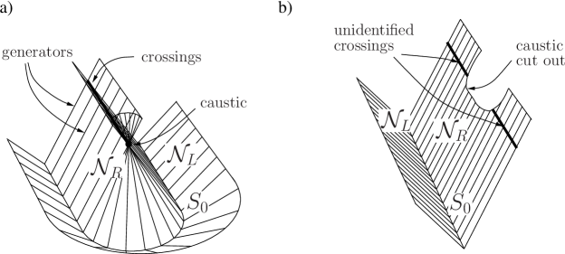
Figure 2: Panel a) shows a simple example of a caustic and intersections of generators in $2+1$ Minkowski space: $S_{0}$ is a spacelike curve having the shape of a half racetrack - a semicircle extended at each end by a tangent straight line. The congruence of null geodesics normal to $S_{0}$ and directed inward and to the future sweep out ${\cal N}_{R}$, which takes the form of a ridge roof, terminated by a half cone over the semicircle. The generators from the semicircle form a caustic at the vertex of the cone. There neighbouring generators intersect. On the other hand generators from the two straight segments of $S_{0}$ cross on a line (the ridge of the roof) starting at the caustic, but the generators that cross there are not neighbours at $S_{0}$. Clearly the generator segments beyond the crossing points enter the interior of the domain of dependence of ${\cal N}$. In Panel b) the double null sheet defined by $S_{0}$ in the covering space is shown, with the points that are identified in the original spacetime indicated.

The remainder of this introduction outlines how these issues are resolved, and how the Poisson bracket on initial data will be defined here. First let us consider caustics and generator crossings, two related but distinct fenomena. At a caustic point neighboring generators focus, so that the congruence of generators is singular there. This can be detected in the initial data: If the functions $\theta^{1}$ and $\theta^{2}$ on ${\cal N}$ form a chart on the disk $S_{0}$ and are constant along the generators then the matrix of components $h_{pq}$ in the $\theta$ chart of the metric induced on 2-surfaces $S\subset{\cal N}$ transverse to the generators is singular at caustic points. Caustics will be excluded from ${\cal N}$ by allowing only initial data such that $h_{pq}$ is regular everywhere on ${\cal N}$.

The problem of non-neighboring generators crossing is resolved in a completely different manner. Non-neighboring generators can cross even if there are no caustic points on ${\cal N}$. See Figure 2. But when there are no caustics on ${\cal N}$ there exists an isometric covering of a spacetime neighborhood of ${\cal N}$ by a spacetime in which no generators cross. This covering spacetime is (a subset of) the normal bundle of $S_{0}$ equipped with the metric obtained by pulling back the metric of the original spacetime using the exponential map. See [Rei07] appendix B for details. The covering spacetime of course induces the same data on ${\cal N}$ as does the original spacetime. Thus we can (and will) always suppose that the generators segment within ${\cal N}$ do not cross in the spacetimes matching the data given on ${\cal N}$, even though for some data there exist alternative matching spacetimes, obtained by identifying isometric spacetime regions, in which the generators do cross. In fact, we will impose the slightly stronger requierments that any point $p\in{\cal N}$ is causally connected only to points on the generators through $p$ and also that ${\cal N}$ is achronal, because ${\cal N}$ has these properties in the covering spacetime [Rei07] appendix B.

Now let us turn to the issue of representing variations of the solution spacetime metric in terms of the variations of null initial data on ${\cal N}$ when these variations of the spacetime metric do not preserve the nullness of ${\cal N}$. This problem is largely resolved by exploiting the diffeomorphism gauge invariance of GR: one describes a given variation of the spacetime metric by the corresponding variations of null initial data in a gauge equivalent variation of the solution metric which does preserve the nullness of the branches of ${\cal N}$.

This is relevant to the definition of the Poisson brackets of null initial data. In mechanics the Poisson bracket is the inverse of the symplectic form. That is,

$$\delta\phi=\omega[\{\phi,\cdot\},\delta]$$ (1)

for all variations $\delta$ tangent to the space of solutions and all functions $\phi$ on this space. Here $\{\cdot,\cdot\}$ is the Poisson bracket and $\omega$ is the symplectic form, a 2-form on the space of solutions defined in Section 2. (See [LW90].) The definition (1) works also when the system has gauge symmetries, that is when $\omega$ is degenerate [LW90], provided $\phi$ is restricted to gauge invariant functions on the space of solutions. It then defines the Poisson bracket between such gauge invariant functions.

Proceeding analogously in the case of vacuum GR one fixes the diffeomorphism gauge freedom of solutions by requiering that a given hypersurface ${\cal N}$ is always a double null sheet, and imposing further conditions until no diffeomorphism gauge freedom remains, that is, each gauge equivalence class is represented by precisely one allowed solution. The solutions will then always induce null data on ${\cal N}$ and these are, moreover, gauge invariant functions on the space of solutions. (1) defines the Poisson bracket between these gauge fixed data.

In fact not all diffeomorphisms are gauge in the sense of being generated by null vectors of the symplectic form (see (11)). And in particular it is not clear that all variations of the metric are gauge equivalent to variations that preserve the double null sheet character of ${\cal N}$. In other words, the gauge fixing imagined above may be impossible.

To proceed we adopt an apparently completely different approach, based on Peierls’ definition of the Poisson bracket, which in the end leads us back to an equation for the Poisson bracket which is simply a slightly weaker version of the condition (1). The Peierls bracket $\{A,B\}$ between two functions, $A$ and $B$ on the space of solutions is the retarded perturbation in $B$ due to the addition of $\gamma A$ to the action, calculated to first order in the parameter $\gamma$, minus the analogous first order advanced perturbation [Pei52]. It provides an expression for the Poisson bracket in terms of advanced and retarded Green’s functions which does not involve the symplectic form or Cauchy surfaces. It’s simplicity gives it a good claim to being a more fundamental definition than (1) in terms of the symplectic form. Furthermore it agrees with the latter definition when both are defined [Pei52, DeW03].

The Peierls bracket does not provide the Poisson bracket between initial data on ${\cal N}$ directly. It is ambiguous on these data because the advanced and retarded Green’s functions between two points are discontinuous when these points are lightlike separated. However the Peierls bracket is well defined on what we call ”observables”, diffeomorphism invariant functionals $F[g]$ of the metric, with smooth functional derivatives $\delta F/\delta g_{ab}$ of compact support (called the domain of sensitivity of the observable and denoted $\sigma_{F}$). Our approach [Rei08, Rei07] is to look for a Poisson bracket $\{\cdot,\cdot\}_{\bullet}$ on initial data that reproduces the Peierls brackets between observables having domains of sensitivity in the interior of the the causal domain of dependence of ${\cal N}$.

The construction of such observables in vacuum GR is not easy in general, but can be done in principle in most vacuum spacetimes. On generic spacetimes charts can be formed from scalar contractions of the Weyl tensor. If ${\cal N}$ is chosen so that $D[{\cal N}]$ is small enough that it can be covered by an atlas of such charts then it is clear that observables in our sense can be defined in terms of the metric components in this chart, and that these characterize the geometry of the interior, $D[{\cal N}]^{\circ}$, of $D[{\cal N}]$ completely. See [Ko58][BK60] for an approach to observables along these lines. Of course each such observable will work, that is satisfy the definition of observable, only on a limited subset of the space of solutions (see [Kha15] for a discussion), but this is the case for almost all physical observables we know, so it does not disqualify them. Note that the role of observables

Note that observables will ultimately play no direct role in the calculation of the Poisson brackets between initial data presented here. Their role is to motivate the definition adopted for this bracket. The existence of a rich set of observables in generic vacuum spacetimes suffices for this purpose.

Another aspect of the motivating framework that is ultimately not used in obtaining our results is the existence and uniqueness of solutions of the Einstein field equations corresponding to the Sachs/Dautcourt initial data. The expression for the symplectic form in terms of initial data was obtained in [Rei13] without invoking this result, and in the present work it is again unnecessary. In fact, both the symplectic form and the Peierls bracket at a given solution metric $g$ are features of the theory linearized about $g$. Thus only properties of GR linearized about $g$ are needed.

We will see that a Poisson bracket $\{\cdot,\cdot\}_{\bullet}$ on the free null initial data on ${\cal N}$ reproduces the Peierls bracket on observables of the interior of $D[{\cal N}]$ if for any such observable $A$ expressed in terms of the initial data

$$\delta A=\omega_{\cal N}[\{A,\cdot\}_{\bullet},\delta],$$ (2)

for any $\delta$ in the space $L_{g}^{0}$ of smooth variations which satisfy the field equations linearized about $g$ and vanish in a spacetime neighbourhood of $\partial{\cal N}$.

This is just a weakened version of the condition (1) that the Poisson bracket be inverse to the symplectic form. But the restriction that the variations $\delta g_{ab}$ vanish in a neighborhood of $\partial{\cal N}$ makes it possible to express both sides of this equation purely in terms of the free null initial data on ${\cal N}$ and their variations, despite the fact that not all diffeomorphisms are gauge. Specifically, one may add any diffeomorphism generator that vanishes in a neighborhood of $\partial{\cal N}$ to $\delta$ and any diffeomorphism generator at all to $\{A,\cdot\}_{\bullet}$ without changing the value of either side of the equation. This allows one to restrict both arguments of $\omega_{\cal N}$ in (2) to what are called “admissible variations“ in [Rei13]; in the case of $\delta$, without weakening the condition it imposes on $\{A,\cdot\}_{\bullet}$, and in the case of $\{A,\cdot\}_{\bullet}$ without leaving the space of solutions to this condition.

Admissible variations are smooth variations of the spacetime metric, satisfying the linearized field equations, that leave the branches ${\cal N}_{A}$ swept out by the generators in spacetime invariant (and also satisfy further conditions detailed in A). Admissible variations therefore correspond to variations of null initial data on a fixed hypersurface ${\cal N}$. In fact within $D[{\cal N}]$ they are determined, modulo diffeomorphism generators, by these variations and the Green’s functions for the linearized field equations. See A or [Rei07] Appendix C. It therefore becomes possible to write (2) entirely in terms of null initial data turning it into a condition on the $\bullet$ Poisson brackets of these data:

$$\delta A=\omega_{\cal N}[\{A,\cdot\}_{\bullet},\delta]\ \ \ \forall\>A\ \mbox{observable},\>\delta\in{\cal B}$$ (3)

where ${\cal B}$ is the set of variations of the initial data corresponding to admissible variations in $L_{g}^{0}$, i.e. that vanish in a spacetime neighborhood of $\partial{\cal N}$. The observable $A$ enters (3) only through its linearization about the spacetime metric $g$, $\Delta A=\int_{\sigma_{A}}\delta A/\delta g^{ab}\Delta g^{ab}\varepsilon$ for any solution $\Delta g^{ab}$ to the linearized field equations. (Here $\varepsilon$ is the spacetime metric volume form.) Linearized observables can in turn be expressed as smeared variations of the initial data, with a particular class of smooth smearing functions.

This condition is almost what we need. It is a condition directly on the $\bullet$ bracket of the initial data, but the set ${\cal B}$ of variations of the initial data is not at all easy to characterize, nor is the set of smearing functions on the initial data that correspond to linearized observables. It would be better to have a simpler condition to define $\{\cdot,\cdot\}$.

Another weakness of (3) is that it does not guarantee that the $\bullet$ bracket satisfies the Jacobi relations. If the Poisson bracket is defined as the inverse of the symplectic 2-form then the Jacobi relations follow as a consequence of the fact that the symplectic form is closed, but (3 is weaker than demanding that $\{\cdot,\cdot\}_{\bullet}$ be inverse to $\omega_{\cal N}$. If one solves (3) as a linear equation for the $\bullet$ brackets between the initial data, assuming that $\{\cdot,\cdot\}_{\bullet}$ is a derivation in each of its arguments but not that it satisfies the Jacobi relations, then the result is not unique, and in general does not satisfy the Jacobi relations. For example, the “pre-Poisson bracket” $\{\cdot,\cdot\}_{\circ}$ of [Rei07] satisfies (3) but violates the Jacobi relations.

For these reasons (2) will be replaced by a simpler and stronger set of conditions which implies the original condition as a corollary, and thus that the $\bullet$ bracket reproduces the Peierls bracket on observables, and also yields a unique solution which satisfies the Jacobi relation.

In these new conditions determining the $\bullet$ bracket the set of linearized observables is replaced by a larger set $\Phi$ of smeared initial data, defined by simple smoothness and boundary conditions on the weighting functions; The set of variations ${\cal B}$ is replaced by a larger set ${\cal C}$ of variations of the data, also satisfying simple smoothness and boundary conditions; And finally it will be required that also the variations $\{\varphi,\cdot\}_{\bullet}$ generated by smeared initial data $\varphi$ via the bracket, lie in ${\cal C}$, so that the $\bullet$ bracket in fact is inverse to $\omega_{\cal N}$ restricted to ${\cal C}$. Thus we require that for all $\varphi\in\Phi$

$$\delta\varphi=\omega_{\cal N}[\{\varphi,\cdot\}_{\bullet},\delta]\ \ \ \forall\>\delta\in{\cal C},$$ (4)

and

$$\{\varphi,\cdot\}_{\bullet}\in{\cal C}.$$ (5)

The fact that the bracket thus defined on smeared initial data in $\Phi$ is unique will be demonstrated in Section 6, and that it satisfies the Jacobi relation will proved in Section 2. There is, however, one apparent problem with the system (4, 5): (3 guarantees that the $\bullet$ bracket reproduces the Peierls bracket on observables if $\{A,\cdot\}_{\bullet}$ is admissible for all observables $A$. But all that is obvious from (4, 5) is that $\{A,\cdot\}_{\bullet}\in{\cal C}$, and ${\cal C}$ is not contained in the set ${\cal A}$ of admissible variations of the initial data.

In fact $\{A,\cdot\}_{\bullet}$ is admissible for all observables $A$. To prove this it is enough to show that (5) and the slightly weakened form of (4),

$$\delta\varphi=\omega_{\cal N}[\{\varphi,\cdot\}_{\bullet},\delta]\ \ \ \forall\>\delta\in{\cal C}\cap{\cal A},$$ (6)

suffice to determine $\varphi,\cdot\}_{\bullet}$. Then, we shall see, that there exists for each observable $A$ a manifestly admissible variation of the initial data which satisfies the same conditions as $\{A,\cdot\}_{\bullet}$ and is hence equal to it. One could therefore say that the $\bullet$ bracket is defined by (6) and (5), but it also satisfies (4), which permits an easy proof of the Jacobi relations.

The brackets obtained from these conditions are stated in Section 5. They are identical to the ones anounced in [Rei08].

Notice that while the requierment that the $\bullet$ bracket reproduces the Peierls bracket on observables was used to motivate the conditions (4), (5), and (6), the conditions themselves do not involve the observables. They are simply modified versions of the standard requierment that Poisson bracket be inverse to the symplectic form.

Of course the question arises: To what extent is the $\bullet$ bracket determined by the requierment that it matches the Peierls bracket on observables, and to what extent is it determined by the additional conditions placed on it to arrive at (4, 5)? We will see that the brackets of certain data, the so called ”diffeomorphism data“ (see Section 3), are not determined by the matching to the Peierls brackets of observables of the interior of the domain of dependence at all because these observables not depend on the diffeomorphism data. On the other hand, experience solving weaker forms of the condition (4) suggests that the brackets of the remaining data, the ”geometrical data“ are essentially uniquely determined by the matching. That is, if one assumes a priori that the $\bullet$ bracket has the properties of a Poisson bracket, including the Jacobi relations, then (3) suffices to determine it uniquely on these data. Note, however, that this is not proved.

The $\bullet$ bracket that we obtain (see Section 5) has one strange property. It does not preserve the reality of the metric. That is, the Hamiltonian flow generated by smeared data that is real on real solutions generates an imaginary component of the metric. This is, however, much less serious than it seems at first because the imaginary mode generated in the initial data does not affect observables. It is a shock wave that skims along a branch of ${\cal N}$ without entering the interior of the domain of dependence. See Subsection 5.1.2. Such a shock wave mode is not seen in the analyses of the initial value problem of [Sac62] and [Dau63] because it is excluded by continuity conditions on the data at $S_{0}$ which are, however, not natural for the Poisson bracket on initial data. It is thus interesting that in [FR17] alternative data is found that captures all the information of the data used here, except this mode.

The remainder of the paper is organized as follows: The next section provides the technical underpinning of part of the preceding discussion. The Peierls bracket and the symplectic form are defined and related to each other, and the Jacobi relation is established for brackets satisfying (4, 5). In Section 3 free initial data that will be used are presented, and the spaces of variations ${\cal C}$ and smeared data $\Phi$ are defined. In Section 4 the symplectic form on admissible variations is expressed in terms of the initial data and their variations. This completes the preparation for the calculation of the $\bullet$ brackets of the data. In Section 5 the result of this calculation is presented and discussed. The calculation that leads to these brackets is presented in detail in Section 6. The article closes with reflections on the results obtained.

2 The Peierls bracket on observables and the definition of the Poisson bracket on initial data

Unless otherwise indicated the solution spacetimes we consider will always be smooth ($C^{\infty}$). The double null sheet ${\cal N}$ will also be smooth in the sense that $S_{0}$, ${\cal N}_{L}$, and ${\cal N}_{R}$ are smoothly embedded. (The smoothness of ${\cal N}_{L}$ and ${\cal N}_{R}$ actually follows from the smoothness $S_{0}$ and the spacetime metric, together with the assumptions that ${\cal N}$ is compact and contains neither caustics nor intersections of generators.)

The solution spacetime will also be assumed to be globally hyperbolic. This is not a very strong restriction because we may take as our spacetime a small neighborhood about ${\cal N}$.

At a solution $g$ the Peierls bracket [Pei52] between two observables $A$ and $B$ is

$$\{A,B\}=\Delta_{A}B$$ (7)

where $\Delta_{A}=\delta^{+}_{A}-\delta^{-}_{A}$, and $\delta^{\pm}_{A}$ is the retarded ($+$)/advanced ($-$) first order perturbation of $g$ due to the addition of a source term $\gamma A$ to the action, with $\gamma$ the perturbation parameter. That $\delta^{+}_{A}$ is retarded means that the support of $\delta^{+}_{A}g_{ab}$ is contained in the causal future $J^{+}[\sigma_{A}]$ of the domain of sensitivity $\sigma_{A}$ of $A$, and similarly the advanced perturbation is supported in the causal past $J^{-}[\sigma_{A}]$ of $\sigma_{A}$.

$\delta^{\pm}_{A}g_{ab}$ are solutions to the linearized field equation with source $\delta A/\delta g_{cd}$, and may be obtained from the retarded/advanced Green’s function. The definition of $\delta^{\pm}_{A}g_{ab}$ requiers the choice of a gauge, which we will take to be de Donder gauge, but the Peierls brackets of observables are independent of this choice. The Peierls bracket is well defined between all observables of $D[{\cal N}]$ and has all the properties of a Poisson bracket [DeW03].

Note that since spacetime is assumed to be globally hyperbolic with a smooth metric, and the linearized vacuum Einstein equations in de Donder gauge are normally hyperbolic $\delta^{\pm}_{A}g_{ab}$ amd $\Delta_{A}g_{ab}$ are smooth [BGP07].

Note also that these perturbations, and thus the Peierls bracket, depends only on the linearized field equations and the linearized observables, or equivalently the functional derivatives $\delta A/\delta g_{cd}$ of the observables. The definition of the Peierls bracket and the general properties we have mentioned require only that these functional derivatives be smooth, compactly supported, symmetric tensor fields with vanishing divergence, $\nabla_{a}\delta F/\delta g_{ab}=0$ (the latter being a consequence of the diffeomorphism invariance of $F$). They are therefore valid not only for observables, but for all linear observables, functionals of the variations $\delta g^{ab}$ of the metric about $g$ of the form $\int\theta^{ab}\delta g^{ab}\varepsilon$, with $\theta^{ab}$ a smooth, compactly supported, symmetric tensor field with vanishing divergence.

This will apply quite generally to all our results involving observables: they hold just as well if we replace the set of observables with the set of linear observables. Linear observables, which include the linearizations of the full observables as a subset, may be thought of as the observables of the linearized theory.

The symplectic form is determined by the action. We shall adopt the Hilbert action,

$$I=\frac{1}{16\pi G}\int_{Q}R\varepsilon,$$ (8)

where $Q$ is the chosen domain of integration and $\varepsilon$ is the metric spacetime volume form. The sign conventions for the curvature tensor and scalar are those of [Wald84], that is, $R=R_{ab}{}^{ab}$ with $[\nabla_{a},\nabla_{b}]\beta_{c}=R_{abc}{}^{d}\beta_{d}$ for any 1-form $\beta$.

The variation of the action due to a variation $\delta$ of the metric consists of a bulk term, which vanishes on solutions, and a boundary term

$$\phi[\delta]=-\frac{1}{8\pi G}\int_{\partial Q}\delta\Gamma^{[c}_{cb}g^{a]b}\varepsilon_{a\cdot\cdot\cdot},$$ (9)

where the dots represent uncontracted abstract indices, that is, the integrand is a 3-form. Restricting this boundary integral to a portion $\Sigma$ of $\partial Q$ one obtains the symplectic potential, $\Theta_{\Sigma}[\delta]$, of $\Sigma$. We will be interested in the case in which $\Sigma$ is the double null sheet ${\cal N}$.

The presymplectic form on field histories, evaluated on a pair of variations $\delta_{1}$ and $\delta_{2}$, is

$$\Omega_{\Sigma}[\delta_{1},\delta_{2}] \equiv \delta_{1}\Theta_{\Sigma}[\delta_{2}]-\delta_{2}\Theta_{\Sigma}[\delta_{1}]-\Theta_{\Sigma}[[\delta_{1},\delta_{2}]]$$

$$= -\frac{1}{8\pi G}\int_{\Sigma}\delta_{2}\Gamma^{[c}_{cb}\delta_{1}(g^{a]b}\varepsilon_{a\cdot\cdot\cdot})-(1\leftrightarrow 2)$$

[CW87]. $\Omega_{\Sigma}$ can be interpreted as the curl (exterior derivative) of $\Theta_{\Sigma}$ in the space of metric fields, contracted with two tangent vectors, $\delta_{1}$ and $\delta_{2}$, to this space. (See [AMR03] for the definition of exterior differentiation in the infinite dimensional context.)

The field histories on which $\Omega_{\Sigma}$ is defined need not satisfy the field equations, nor need the variations preserve these field equations. Restricting $\Omega_{\Sigma}$ to metrics that satisfy the field equation and variations $\delta_{1}$, $\delta_{2}$ that satisfy the linearized field equations one obtains $\omega_{\Sigma}$, the presymplectic form on the space of solutions. Here the space $L_{g}$ of smooth solutions to the field equations linearized about the metric $g$ plays the role played by the tangent space to the phase space in the definition of the presymplectic form in finite dimensional mechanics.

The degeneracy vectors of the presymplectic form on the space of solutions are variations $\gamma$ such that $\omega_{\Sigma}[\cdot,\gamma]=0$. These generate the gauge transformations of the system in the domain of dependence of $\Sigma$ [LW90]. Lie derivatives, which generate diffeomorphisms, are degeneracy vectors of the presymplectic form on the space of solutions of vacuum gravity defined by 2. Suppose $\delta$ is an arbitrary variation in $L_{g}$ and $\xi$ is a smooth vector field then $\pounds_{\xi}\in L_{g}$, because the space of solutions is diffeomorphism invariant, and [Rei13]

$$\omega_{\cal N}[\pounds_{\xi},\delta]=\frac{1}{16\pi G}\int_{\partial{\cal N}}3\xi^{[a}\delta\Gamma^{c}_{cd}g^{b]d}\varepsilon_{ab\cdot\cdot}+\delta[g^{ca}\varepsilon_{ab\cdot\cdot}]\nabla_{c}\xi^{b}.$$ (11)

It follows that any $\xi$ that vanishes on $\partial{\cal N}$ and has vanishing derivatives there generates gauge diffeomorphisms, but some other diffeomorphisms, generated by $\xi$ which have non-zero values or derivatives on ${\cal N}$ are not gauge.

The preceding results apply to more or less arbitrary compact hypersurfaces with boundary, $\Sigma$, in spacetime, and in particular to the case that $\Sigma$ is a double null sheet ${\cal N}$. Equation (11) therefore demonstrates the equivalence of (2) and (3) because $\omega_{\cal N}[\pounds_{\xi},\delta]=0$ for any $\delta\in L_{g}$ if $\xi=0$ in a neighborhood of $\partial{\cal N}$, and for any $\xi$ if $\delta\in L_{g}^{0}$.

In standard terminology a symplectic form is a presymplectic form that has no non-zero degeneracy vectors. But of course whether or not it has non-zero degeneracy vectors depends on the variables used to describe the system. Since it is always in a sense “the same” object the author prefers to refer to it from here on as the symplectic form of the system, independently of the variables used and whether or not it has degeneracy vectors.

Note that in the calculation of the symplectic form no boundary term has been added to the Hilbert action because such a boundary term would not affect the Peierls bracket, since it does not affect the advanced and retarded Green’s functions. At first sight it also seems that it would not affect the symplectic form either because it contributes only a total variation to the boundary term $\phi[\delta]$ in the variation of the action, and thus, apparently, to the symplectic potential. However, $\phi[\delta]$ determines its integrand only up to an exact form, and thus the symplectic potential $\Theta_{\cal N}$ only up to a $\partial{\cal N}$ boundary term. Depending on the prescription chosen for determining the integrand of $\phi[\delta]$ a boundary term in the action may or may not contribute a boundary term to $\omega_{\cal N}$ [LW90]. A change in $\omega_{\cal N}$ could in turn affect the $\bullet$ bracket on initial data since this bracket will ultimately be defined by the symplectic form, via conditions (4) and (5). However, whatever the boundary term in the action and whatever the prescription used to determine the integrand of $\phi[\delta]$, the $\bullet$ bracket we obtain will reproduce the same Peierls bracket. Since this is all that is required of the $\bullet$ bracket the simplest option is adopted: no boundary term is added to the Hilbert action, and the integrand of $\phi[\delta]$ is as indicated in (9).

The symplectic form is closely related to the Peierls bracket. Let $A$ and $B$ be two (full or linear) observables of the interior of the domain of dependence of ${\cal N}$, that is, having domains of sensitivty in $D[{\cal N}]^{\circ}$, and let us choose the domain of integration $Q$ of the action so that it is bounded to the past by ${\cal N}$ and to the future by another achronal hypersurface, and contains the domains of sensitivity of $A$ and $B$ in its interior. At stationary points of the action $\delta I-\phi[\delta]=0$ for any variation $\delta$. (In vacuum GR this is $G_{ab}\delta g^{ab}=0$, with $G$ the Einstein curvature.) Thus, if a variation $\delta_{0}$ preserves the field equations then

$$\delta_{0}\delta I=\delta_{0}\phi[\delta],$$ (12)

which is equivalent to the linearized field equation $\delta_{0}G_{ab}=0$.

Now consider the perturbed action $I+\gamma A$. If there were an exact power series solution $g+\gamma\delta_{A}g+...$ of the corresponding field equations, then at the first order aproximate solution $g+\gamma\delta_{A}g$

$$\delta I+\gamma\delta A-\phi[\delta]=o(\gamma)$$ (13)

for any variation $\delta$, where $o(\gamma)$ vanishes more rapidly than $\gamma$ as $\gamma\rightarrow 0$. Note that the boundary term $\phi[\delta]$ in the variation is the same as for the unperturbed action since $\delta A/\delta g_{ab}$ vanishes in a neighborhood of $\partial Q$.

This equation is taken as the definition of first order solutions, even when no corresponding exact power series solution exists. It is equivalent to an order zero equation obtained by setting $\gamma=0$, which requires $g$ to be a stationary point of the unperturbed action, and an order one equation obtained by taking the derivative in $\gamma$ at $\gamma=0$:

$$\delta_{A}\delta I+\delta A-\delta_{A}\phi[\delta]=0.$$ (14)

This is just the linearized field equation with a source term, $[16\pi G]^{-1}\delta_{A}G_{ab}+\delta A/\delta g^{ab}=0$.

Putting $\delta=\delta_{0}$ in (14) and $\delta=\delta_{A}$ in (12), and subtracting the two one obtains

$$\delta_{0}A=\delta_{A}\phi[\delta_{0}]-\delta_{0}\phi[\delta_{A}]-\phi[[\delta_{A},\delta_{0}]].$$ (15)

This equation applies in particular to the retarded and advanced parturbations $\delta^{\pm}_{A}$ that appear in the definition of the Peierls bracket. But $\delta^{+}_{A}$, being retarded, vanishes on ${\cal N}$, while the support of $\delta^{-}_{A}$ on $\partial Q$ is contained in $J^{-}[\sigma_{A}]\cap\partial Q$ which lies entirely in the interior of ${\cal N}$ [Rei07] (prop. B.21). Consequently $\Omega_{{\cal N}}[\delta^{+}_{A},\delta_{0}]=0$ and

$$\delta^{-}_{A}\phi[\delta_{0}]-\delta_{0}\phi[\delta^{-}_{A}]-\phi[[\delta^{-}_{A},\delta_{0}]]=-(\delta^{-}_{A}\Theta_{{\cal N}}[\delta_{0}]-\delta_{0}\Theta_{{\cal N}}[\delta^{-}_{A}]-\Theta_{{\cal N}}[[\delta^{-}_{A},\delta_{0}]])=-\Omega_{{\cal N}}[\delta^{-}_{A},\delta_{0}],$$ (16)

where the minus arises because we take ${\cal N}$ to be future oriented, while $\partial Q$ is past oriented where it coincides with ${\cal N}$. Thus (15) implies

$$\delta_{0}A=\Omega_{{\cal N}}[\delta^{+}_{A},\delta_{0}]-\Omega_{{\cal N}}[\delta^{-}_{A},\delta_{0}]=\omega_{\cal N}[\Delta_{A},\delta_{0}],$$ (17)

an equation valid for $\delta_{0}$ any solution to the linearized field equations. Note that by (14) $\Delta_{A}=\delta^{+}_{A}-\delta^{-}_{A}$ also satisfies the linearized field equation (12).

We are now in a position to demonstrate that (2) is sufficient to ensure that the $\bullet$ bracket reproduces the Peierls bracket on observables. Suppose $\{\cdot,\cdot\}_{\bullet}$ is a Poisson bracket on the free null initial data such that for any observable $B$, expressed in terms of initial data, the variation of initial data $\{B,\cdot\}$ corresponds to a smooth solution of the linearized field equations, which will also be denoted $\{B,\cdot\}$. Then (17), and the antisymmetry of the $\bullet$ Poisson bracket and the symplectic form, imply that

$$\{A,B\}_{\bullet}=-\{B,A\}_{\bullet}=-\omega_{\cal N}[\Delta_{A},\{B,\cdot\}_{\bullet}]=\omega_{\cal N}[\{B,\cdot\}_{\bullet},\Delta_{A}].$$ (18)

for all observables $A$ and $B$.

On the other hand, by definition the Peierls bracket is $\{A,B\}=\Delta_{A}B$, so the $\bullet$ bracket reproduces the Peierls bracket on observables if and only if

$$\Delta_{A}B=\omega_{\cal N}[\{B,\cdot\}_{\bullet},\Delta_{A}].$$ (19)

But $\Delta_{A}\in L_{g}^{0}$, since the support of $\delta^{\pm}_{A}$, contained in $J^{\pm}[\sigma_{A}]$, is disjoint from a neighborhood of $\partial{\cal N}$ [Rei07] (prop. B.21). It follows that (2) implies (19).

Note that the preceding argument only involves the linearizations of the observables. The result applies to all linear observables which can be expressed in terms of the variations of the initial data about those of the reference solution $g$: For any pair of such linear observables (2) guarantees that $\{A,B\}_{\bullet}=\{A,B\}$.

In fact, all linear observables of $D[{\cal N}]^{\circ}$ may be expressed in terms of the variations of the initial data. For $A$ any such linear observable $\Delta_{A}$ lies in $L_{g}^{0}$, so it can be made admissible by a suitable adjustment of gauge, specifically, by addition of a diffeomorphism generator that vanishes in a neighborhood of $\partial{\cal N}$. (See A.) Let us suppose from here on that this has been done. This of course leaves (17) unchanged. If $\delta_{0}$ is also required to be admissible, then the right side of (17) is expressible in terms of the free initial data and their variations. Indeed, (17) becomes the sought for expression for the linear observable $A[\delta]\equiv\delta A$ in terms of the variations of the initial data. It is valid on the set ${\cal A}$ of variations of the initial data that correspond to admissible variations, described in detail in A.

This also allows us to verify that the linear observable $A$ is contained in the space $\Phi$ of smeared data. Since $\Delta_{A}$ is admissible and vanishes in a neighborhood of $\partial{\cal N}$ the variation of the initial data it defines belongs to ${\cal B}\subset{\cal A}$. It thus satisfies all the smoothness conditions of variations in ${\cal A}$ described in A and also vanishes in a neighborhood of $\partial{\cal N}$ in ${\cal N}$. It is then straightfoward to check that $\omega_{\cal N}[\Delta_{A},\delta]$, for $\delta$ admissible, is a smearing of the variations under $\delta$ of the initial data with weighting functions that satisfy the smoothness and boundary conditions that define $\Phi$, given in Definition 2.

Now let us consider the conditions (6) and (5). In the Introduction these were presented as the last in a chain of sufficient conditions for the agreement on observables between the $\bullet$ bracket and the Peierls bracket, starting with (2), in order to introduce the ideas one at a time. It is not difficult to show that (6) and (5) imply the other sufficient conditions in the chain, but it is easier still to show directly that they imply the matching of $\bullet$ and Peierls brackets.

The key result is that if $\{\cdot,\cdot\}_{\bullet}$ satisfies (6) and (5) for all $\varphi\in\Phi$ then for all linear observables $A$

$$\{A,\cdot\}_{\bullet}=\Delta_{A}$$ (20)

on initial data. In Section 6 it is shown that (6) and (5) define $\{\varphi,\cdot\}_{\bullet}$ uniquely for all $\varphi\in\Phi$ and thus in particular they define $\{A,\cdot\}_{\bullet}$ uniquely. On the other hand $\Delta_{A}$ satisfies the same conditions as $\{A,\cdot\}_{\bullet}$: ${\cal B}$ is a subset of ${\cal C}$ as can be seen from the definition of ${\cal C}$ in Subsection 3.6, so $\Delta_{A}$ satisfies(6) and (5) (5), and by (17) it also satisfies (6). This establishes (20).

The result (20) shows that $\{A,\cdot\}_{\bullet}\in{\cal A}$, as claimed in the Introduction. It also shows immediately that the $\bullet$ bracket reproduces the Peierls bracket on observables: $\{A,B\}\equiv\Delta_{A}B=\{A,B\}_{\bullet}$ for all linear observables $A$, $B$ (and thus a fortiori for all full observables).

In Section 6 it is also demonstrated that the bracket that satisfies (6) and (5) for all $\varphi\in\Phi$ satisfies (4) as well for all these $\varphi$. This makes it easy to prove that the $\bullet$ bracket satisfies the Jacobi relations

$$\{\alpha,\{\beta,\gamma\}_{\bullet}\}_{\bullet}+\{\gamma,\{\alpha,\beta\}_{\bullet}\}_{\bullet}+\{\beta,\{\gamma,\alpha\}_{\bullet}\}_{\bullet}=0\ \ \ \forall\>\alpha,\beta,\gamma\in\Phi$$ (21)

In finite dimensional mechanics the Poisson bracket $\{\phi,\theta\}$ is a bilinear on the differentials $d\phi$, $d\theta$ of its arguments (or equivalently a derivation on each argument) and inverse to the symplectic form, which is closed, and this implies that it satisfies the Jacobi relation. The following proposition provides an analogous result for a bracket $\{\cdot,\cdot\}_{\bullet}$ satisfying (4) and (5).

Proposition 1

If $\{\cdot,\cdot\}_{\bullet}$ is a derivation on each of its arguments defined on a domain that includes $\Phi$ and also $\{\varphi_{1},\varphi_{2}\}_{\bullet}$ for all $\varphi_{1},\varphi_{2}\in\Phi$, and

$$\delta\varphi=\omega_{\cal N}[\{\varphi,\cdot\}_{\bullet},\delta]\ \ \ \ \mbox{and}\ \ \ \{\varphi,\cdot\}_{\bullet}\in{\cal C}\ \ \forall\>\delta\in{\cal C},\varphi\in\Phi.$$ (22)

then $\{\cdot,\cdot\}_{\bullet}$ satisfies the Jacobi relations.

Proof: By (22) $\{\varphi_{1},\varphi_{2}\}_{\bullet}=-\omega_{\cal N}[\{\varphi_{1},\cdot\}_{\bullet},\{\varphi_{2},\cdot\}_{\bullet}\}]$. On the other hand (2) restricted to variations in ${\cal C}$ implies that $\vtop{\halign{#\cr$\textstyle{\rm Cyc}$\crcr\kern-1.72218pt\nointerlineskip\cr{\tiny i,j,k}\crcr}}\ \delta_{i}\omega_{\cal N}[\delta_{j},\delta_{k}]=\vtop{\halign{#\cr$\textstyle{\rm Cyc}$\crcr\kern-1.72218pt\nointerlineskip\cr{\tiny i,j,k}\crcr}}\ \omega_{\cal N}[[\delta_{i},\delta_{j}],\delta_{k}]$ for all $\delta_{1},\delta_{2},\delta_{3}\in{\cal C}$, where Cyc indicates a cyclic sum. (In differential terms, $\omega_{\cal N}$ is a closed form because it is the curl of $\Theta_{\cal N}$.) Thus, letting $X=\vtop{\halign{#\cr$\textstyle{\rm Cyc}$\crcr\kern-1.72218pt\nointerlineskip\cr{\tiny i,j,k}\crcr}}\ \{\varphi_{i},\{\varphi_{j},\varphi_{k}\}_{\bullet}\}_{\bullet}$ and $\Delta_{i}=\{\varphi_{i},\cdot\}_{\bullet}$ for $i=1,2,3$,

$$X = -\vtop{\halign{#\cr$\textstyle{\rm Cyc}$\crcr\kern-1.72218pt\nointerlineskip\cr{\tiny i,j,k}\crcr}}\ \Delta_{i}\omega_{\cal N}[\Delta_{j},\Delta_{k}]=-\vtop{\halign{#\cr$\textstyle{\rm Cyc}$\crcr\kern-1.72218pt\nointerlineskip\cr{\tiny i,j,k}\crcr}}\ \omega_{\cal N}[[\Delta_{i},\Delta_{j}],\Delta_{k}]$$ (30)

$$=\vtop{\halign{#\cr$\textstyle{\rm Cyc}$\crcr\kern-1.72218pt\nointerlineskip\cr{\tiny i,j,k}\crcr}}\ [\Delta_{i},\Delta_{j}]\varphi_{k}.$$

But then $X=\vtop{\halign{#\cr$\textstyle{\rm Cyc}$\crcr\kern-1.72218pt\nointerlineskip\cr{\tiny i,j,k}\crcr}}\ \{\varphi_{i},\{\varphi_{j},\varphi_{k}\}_{\bullet}\}_{\bullet}-\{\varphi_{j},\{\varphi_{i},\varphi_{k}\}_{\bullet}\}_{\bullet}=2X$, so $X=0$, which is precisely the Jacobi relation. 

Notice that the first equation in the proof, $\{\chi,\varphi\}_{\bullet}=\omega_{\cal N}[\{\varphi,\cdot\}_{\bullet},\{\varphi,\cdot\}_{\bullet}]$ shows that the $\bullet$ bracket is antisymmetric as a consequence of (4, 5), so a biderivation satisfying (4) and (5) automatically has all the properties of a Poisson bracket.

3 The free data

The data will be referred to charts $(v_{A},\theta^{1},\theta^{2})$ constructed on each branch ${\cal N}_{A}$ of ${\cal N}$ from a common smooth chart $(\theta^{1},\theta^{2})$ on $S_{0}$: The coordinates $\theta^{1}$ and $\theta^{2}$ are extended to ${\cal N}_{A}$ by holding them constant along the generators, and the coordinate $v_{A}$ parametrizes each generator. Since $\partial_{v_{A}}$ is then tangent to the generators and hence null, and also normal to ${\cal N}_{A}$ (see [Rei13] for a proof), the line element on ${\cal N}_{A}$ takes the form

$$ds^{2}=h_{pq}d\theta^{p}d\theta^{q}$$ (31)

with no $dv$ terms. $v_{A}$ is taken to be proportional to the square root of $\rho\equiv\sqrt{\det h}$, the area density in $\theta$ coordinates on two dimensional cross sections of ${\cal N}_{A}$, and normalized to $1$ at $S_{0}$. Thus $\rho(v_{A},\theta^{1},\theta^{2})=\rho_{0}(\theta^{1},\theta^{2})v_{A}^{2}$, with $\rho_{0}$ the area density on $S_{0}$. The coordinate $v$ will be called the area parameter. (The index $A$ specifying the branch ${\cal N}_{A}$ that a quantity pertains to will often be dropped when there is little risk of confusion.)

3.1 Geometrical data

The free initial data we will use consists of geometrical data and diffeomorphism data. The geometrical data are:

1. The conformal 2-metric $e_{pq}=h_{pq}/\rho$ given as a function of the $v\theta$ chart on ${\cal N}_{L}$ and ${\cal N}_{R}$. $e$ is a unit determinant, symmetric, $2\times 2$ matrix, which captures the equivalence class with respect to local rescalings of the induced metric $h_{pq}$ on the branches of ${\cal N}$. It is the only datum which is given on all of ${\cal N}$.

2. Three fields specified on $S_{0}$ only, as functions of $(\theta^{1},\theta^{2})$:

   • $\rho_{0}$,

   • $\lambda=-\ln|n_{L}\cdot n_{R}|$,

   and

   • the twist

     $$\tau_{p}=\frac{n_{L}\cdot\nabla_{p}n_{R}-n_{R}\cdot\nabla_{p}n_{L}}{n_{L}\cdot n_{R}}.$$ (32)

   Here $n_{A}=\partial_{v_{A}}$ is the tangent to the generators of ${\cal N}_{A}$, and inner products ($\cdot$) are taken with respect to the spacetime metric.

An advantage of using $v\equiv\sqrt{\rho/\rho_{0}}$ as the parameter along generators is that it makes excluding caustics easy. It suffices to require that $e_{pq}$ be non-singular and $v>0$ on ${\cal N}$. For then $h_{pq}=\rho_{0}v^{2}e_{pq}$ is non-singular on ${\cal N}$. ($\rho_{0}>0$ is a consequence of $S_{0}$ being spacelike and $(\theta^{1},\theta^{2})$ being a good chart.)

But $v$ is not always a good parameter on generators. For instance, it fails in the important special case in which ${\cal N}_{A}$ is a null hyperplane in Minkowski space, because the generators neither converge nor diverge, resulting in a $v$ that is constant on each generator. On the other hand, it is a good parameter in several important cases: In the case of greatest interest from the point of view of the holographic entropy bound, in which the generators of ${\cal N}_{A}$ are converging everywhere on $S_{0}$ ($dv_{A}$ negative along the generators in direction toward $S_{A}$), the vacuum field equations guarantee that $v_{A}$ continues to decrease right up to the trunction surface $S_{A}$. (See [Wald84] Section 9.2.)

The area parameter $v$ is also a good parameter if the generators are all diverging at $S_{0}$, provided the generators are truncated before they stop diverging. Finally, even if the expansion of the generators has a definite sign only on a patch of $S_{0}$ one can define a new, smaller double null sheet formed by the generators through this patch, and thus define the $\bullet$ bracket on these generators. This is more significant than it might seem because all the brackets between data living on different generators are expected to vanish. This expectation comes from the micro-causality principle, which requires the bracket between fields at causally unconnected points to commute, and the fact that on ${\cal N}$ only points lying on the same generator are causally connected, points on different generators being spacelike to each other. (see [Rei07] prop. B.7.) Micro-causality is an important property of commutators in quantum field theory, and the Peierls bracket also satisifies it in the sense that only observables with causally connected domains of sensitivity have non-zero Peierls bracket. And in fact, the $\bullet$ bracket does satisfy micro-causality on those double null sheets for which it has been calculated, that is, those on which $v$ is a good parameter.

It is therefore without too great a loss of generality that we limit attention to double null sheets consisting of branches on which $v_{A}$ is everywhere increasing, or everywhere decreasing as one moves away from $S_{0}$ along the generators.

Sachs [Sac62] and Dautcourt [Dau63] have argued that a set of data quite similar to our geometrical data is free, and complete in the sense that any valuation of their data determines a matching solution metric uniquely up to diffeomorphisms. In fact it has been proved by Rendall that any smooth Sachs Dautcourt (SD) data matches a unique smooth solution in some neighbourhood of $S_{0}$ [Ren90], and, by the arguments of [Sac62] and [Dau63] it is a reasonable conjecture that it matches a unique smooth solution on all of ${\cal N}$, provided ${\cal N}$ is free of caustics.

In [Rei13] it is demonstrated that if our geometrical data are smooth on their domains, with $e$ continuous at $S_{0}$, then they are equivalent to similarly smooth valuations of the SD data, in the sense that a solution matches our data if and only if it matches the corresponding SD data. Our geometrical data are thus as free and complete as the SD data.

3.2 Diffeomorphism data

In addition to the geometrical data there are diffeomorphism data. As mentioned earlier, not all diffeomorphisms are gauge in canonical GR on ${\cal N}$. Some infinitesinmal diffeomorphisms which are non-trivial at the boundary $\partial{\cal N}$ are not degeneracy vectors of the symplectic form (see (11)). It should thus come as no surprise that some diffeomorphism data, that measure these non-gauge diffeomorphisms, are needed to express the symplectic 2-form. These are

• $s_{A}^{k}$, $A\in\{L,R\},k\in\{1,2\}$ given as a function of the $\theta$ chart. $s_{A}^{k}(\theta)$ is the position of the end point on $S_{A}$ of the generator labeled by $(\theta^{1},\theta^{2})$ in fixed, smooth coordinates $y^{k}_{A}$ on $S_{A}$. That is, it is the transformation from the $\theta$ chart to the $y_{A}$ chart.

A fixed chart is one that is, so to speak, “painted on the manifold”, unlike moving charts like Riemann normal coordinates or our $v\theta$ chart, which change at a given point when the metric field changes. Recall that a manifold consists of a set of a priori identifiable points and an atlas of charts on these. These charts are the fixed charts. For any given metric field the moving charts are also identified with elements of this atlas, but the element depends on the metric. Fixed charts are important for the concept of the variation of a field, since they facilitate the comparison of different valuations of a field at the same point, and of course they are necessary for the description of the gauge equivalence classes of solutions if not all diffeomorphisms are gauge. See the appendix of [Rei13] for a more detailed discussion of fixed and moving charts.

The $s_{A}^{k}$ are independent of of each other and of the geometrical data: Imagine that the spacetime metric is acted on by a diffeomorphism that leaves a neighborhood of $S_{0}$ fixed. This leaves the geometrical data, given as functions of the $v\theta$ charts, unchanged. But the congruences of null geodesics normal to $S_{0}$ are carried along by the diffeomorphism of the metric, so the $s_{A}^{k}(\theta)$ can be changed to any desired value by means of such a diffeomorphism.

The data $s_{A}$ are not enough to specify all the non-gauge diffeomorphism degrees of freedom. But recall that in equation 2, which assures that the $\bullet$ bracket on the data reproduces the Peierls bracket on observables, the variations can be restricted to only admissible ones. The non-gauge diffeomorphism generators in this space are determined by $s_{A}^{k}$, the geometric data, and their variations, as can be seen from the fact that the symplectic form on admissible variations can be expressed entirely in terms of the variations of $s_{A}^{k}$ and of the geometric data [Rei13]. (See equations (45 - 47).)

The diffeomorphism equivalence class of the solution to the field equations corresponding to the data is independent of the diffeomorphism data, and so are, therefore, the diffeomorphism invariant observables. The condition that the $\bullet$ bracket reproduces the Peierls brackets of the observables thus does not involve the diffeomorphism data at all. This means that (2) cannot tell us anything about the brackets of $s^{k}_{A}$. The fact that our calculation nevertheless fixes the brackets of $s^{k}_{A}$ with all the data is due to the fact that we strengthen (2) to get a definite solution. It also means that the conditions that (2) places on the brackets of the geometric data cannot involve the diffeomorphism data. In fact, under the $\bullet$ bracket we obtain the geometrical data form a closed Poisson algebra among themselves: the brackets between the geometrical data do not depend on $s^{k}_{A}$. This closed subalgebra is the main result derived in the present paper.

Should the diffeomorphism data then be discarded as irrelevant? If we take the point of view that the observables, or the geometry, of the interior of the domain of dependence is all that is “physical” then the datum $s^{k}_{A}$, and its $\bullet$ bracket are indeed superfluous. Only the geometrical data and their brackets matter. But the diffeomorphism data ought to be important when a wider context than just the interior of the domain of dependence is considered, because they encode non-gauge information about the boundary of ${\cal N}$. Their role may be analogous to that of the center of mass coordinates in an isolated mechanical system, which are not gauge but are superfluous to a description of the internal dynamics of the system. In fact the author expects that the non-gauge diffeomorphism degrees of freedom will be associated to quasi-local charges, such as linear and angular momentum, for ${\cal N}$.

Here the data $s_{A}^{k}$ will be retained because this is natural in our formalism. They play a central role in the calculation of the symplectic form in [Rei13] and also in the calculation of the $\bullet$ bracket here, even though they ultimately play no role in the brackets of the geometrical data.

One more pair of data fields is needed to express the symplectic form on admissible variations, namely

• $\dot{v}_{A}(\theta^{1},\theta^{2})$, $A=L,R$, the value of $v$ on the truncating surfaces of the two branches.

Under admissible variations $\dot{v}_{A}$ can vary, but its variation is determined by those of the other data because admissible variations maintain $\dot{\rho}_{A}$, the $y_{A}$ chart area density on $S_{A}$, invariant (see A), and

$$\dot{v}_{A}(\theta)=\sqrt{\frac{\dot{\rho}_{A}(s_{A}(\theta))|\det[\partial s_{A}/\partial\theta]|}{\rho_{0}}}.$$ (33)

It is therefore possible, and in fact natural, to write the symplectic form on admissible variations without the appearance of variations of $\dot{v}$.

$\dot{v}_{A}$, like $s_{A}^{k}$, does not affect the spacetime geometry, although it does affect the shape of the domain of dependence of ${\cal N}$ in spacetime. It is really another diffeomorphism degree of freedom which, like the other data, can be specified freely, but since it is equivalent to $\dot{\rho}_{A}$, which is frozen, it does not vary independently of these under admissible variations. $\bullet$ brackets for $\dot{v}_{A}$ can be calculated from (33) and the brackets of the other data, but it is not clear what the significance of these brackets is.

3.3 Summary of free data and smoothness conditions

These are all our free initial data. To summarize, they consist of

• 10 real $C^{\infty}$ functions, $\rho_{0}$, $\lambda$, $\tau_{p}$, $\dot{v}_{A}$, and $s_{A}^{k}$, on a domain $D\in\mathbb{R}^{2}$ having the topology of a closed disk, with $\rho_{0}>0$ and $\dot{v}_{A}>0$ and $\neq 1$

• two $C^{\infty}$, real, symmetric, unit determinant $2\times 2$ matrix valued functions ($e_{pq}$ on ${\cal N}_{L}$ and ${\cal N}_{R}$) on the domains $\{(v_{a},\theta^{1},\theta^{2})\in\mathbb{R}^{3}|\theta\in D,\min(1,\dot{v}_{A}(\theta))\leq v_{A}\leq\max(1,\dot{v}_{A}(\theta))\}$, $A=L,R$ which match at $v_{L}=v_{R}=1$ (i.e. on $S_{0}$).

Our phase space is the space of valuations of these data.

The smoothness and continuity conditions on the data, and the inequalities on $\rho_{0}$ and $\dot{v}$, “regularity” conditions for short, follow from the assumed properties of the spacetime geometry, of ${\cal N}$ and its generators, and of the charts used: $\rho_{0}(\theta)$ is $>0$ and smooth because $S_{0}$ is spacelike and smooth in a smooth spacetime geometry, and $\theta$ is a smooth chart on $S_{0}$. The fact that in a smooth geometry a point on a geodesic depends smoothly on the starting point and tangent of the geodesic, and on the corresponding affine parameter ([HE73] p. 33) ensures that the induced 2-metric components $h_{pq}$ on ${\cal N}$ is a smooth function of $\theta^{1}$, $\theta^{2}$ and an affine parameter on the congruence of generators. It follows that $v=\sqrt{\rho/\rho_{0}}$ is also smooth, which together with the assumed non-stationarity of $v$ along the generators along the generators ensures that the remaining geometrical data on $S_{0}$ is smooth. As to $e$, the non-stationarity of $v$ implies that the induced metric is smooth in $(v,\theta^{1},\theta^{2})$. The absence of caustics on ${\cal N}$ implies that the matrix $h_{pq}$ is everywhere invertible, so $\rho>0$, and thus that $e_{pq}$ is smooth. Finally, the smoothness of $\dot{v}_{A}$ and of $s_{A}$ follows from that of $S_{A}$ and of the fixed chart $y_{A}$, and $\dot{v}\neq 1$ and $\dot{v}>0$ follow from the nonstationarity of $v$ and $\rho>0$ respectively.

Conversely, suppose a model ${\cal N}$ of a double null sheet is chosen in $\mathbb{R}^{4}$, satisfying all the smoothness conditions, and equipped with smooth charts $\theta$, $y_{L}$ and $y_{R}$ on $S_{0}$, $S_{L}$ and $S_{R}$ respectively, and suppose smooth charts $(v_{A},\theta^{1},\theta^{2})$ are chosen such that the $\theta^{p}$ constant curves remain in ${\cal N}_{A}$ from $S_{0}$ to $S_{A}$, and $v_{A}=\dot{v}_{A}(\theta)$ and $y_{A}^{k}=s_{A}^{k}(\theta)$ on $S_{A}$. If regular geometrical data are set on ${\cal N}$ according to these coordinates then in any $C^{1}$ Lorentzian metric spacetime geometry matching the data $S_{0}$ is spacelike because $\rho_{0}e_{pq}$ is a positive definite metric, and ${\cal N}$ is a double null sheet with the predetermined generators, the constant $\theta$ curves, because the tangents to these are null vectors orthogonal to ${\cal N}$ and the vanishing of the torsion of the metric connection implies that their integral curves are geodesics: If $f$ is a smooth function on an open domain in spacetime which vanishes on ${\cal N}$ and $k\equiv df$ is non-zero there then $k^{a}$ is orthogonal to ${\cal N}$ and thus tangent to the generators, and

$$0=2k^{a}\nabla_{[a}\nabla_{b]}f=\nabla_{k}k_{b}-k^{a}\nabla_{b}k_{a}=\nabla_{k}k_{b}-\frac{1}{2}\nabla_{b}k^{2}=\nabla_{k}k_{b},$$ (34)

establishing the claim.

It remains to see whether a spacetime metric matching the data that satisfies the vacuum field equations is necessarily smooth. In [Rei13] it is demonstrated that regular valuations of our geometrical data are equivalent to similarly smooth Sachs Dautcourt data and Rendall has proved that any smooth SD data matches a unique smooth solution in some neighbourhood of $S_{0}$ [Ren90], and, as we said earlier, it is a reasonable conjecture that it matches a unique smooth solution on all of ${\cal N}$. If the conjecture is valid then the regularity of the data implies the smoothness of the spacetime geometry. Thus, modulo this last conjectural element, a complete correspondence has been established between our initial data and a the set of spacetime solution metrics, equipped with double null sheets and $\theta$ and $y$ charts, modulo certain diffeomerphisms.

Note that we will not actually need all of this correspondence, in particular not the conjectured exitence of and uniqueness of smooth solutons matching the data on all of ${\cal N}$. We are calculating the Poisson brackets of the data

3.4 $\theta$ gauge diffeomorphisms and the extension of the phase space

The conditions (4) and (5) define a bracket only between gauge invariant smeared data, or more precisely, on smeared data that are invariant under any degeneracy vector of the restriction of the symplectic form to ${\cal C}$. If $\varphi$ is not gauge invariant in this sense (4, 5) have no solution $\{\varphi,\cdot\}_{\bullet}$, and if it is invariant then $\{\varphi,\cdot\}_{\bullet}$ is determined only up to the addition of degeneracy vectors, so $\{\varphi,\chi\}_{\bullet}$ is defined only if $\chi$ is also gauge invariant.

The geometric data are largely diffeomorphism invariant. They depend on the diffeomorphism equivalence class of the spacetime metric and on a point on $S_{0}$. Admissible diffeomorphisms, that is, diffeomorphisms generated by admissible variations, map ${\cal N}$ and its parts $S_{0}$, $S_{L}$ and $S_{R}$ to themselves, and the effect on the geometric data of such a diffeomorphism of the metric field is equivalent to a change of the $\theta$ chart. The diffeomorphism data $s_{A}$ are affected by both the action of the diffeomorphism on $S_{0}$ and by its action on $S_{A}$, equivalent to an independent change of the $y_{A}$ chart. A change of the $\theta$ chart, suitably restricted on $\partial S_{0}$, can always be produced by a spacetime diffeomorphism that vanishes and has zero gradient at $\partial{\cal N}$, and therefore is gauge according to (11). Indeed it will turn out that any generator of diffeomorphisms of the $\theta$ chart is a degeneracy vector of $\omega_{\cal N}$ restricted to ${\cal C}$. Furthermore, these are the only degeneracy vectors, for once this gauge freedom is fixed, by fixing the $\theta$ chart to the $y_{L}$ chart by setting $s_{L}=id$, the symplectic form $\omega_{\cal N}|_{{\cal C}}$ becomes non-degenerate, as is shown by the existence of a Poisson bracket for the data in precisely this gauge. See Subsection 5.2.

However the gauge fixing $s_{L}=id$ is awkwardly asymmetric between the two branches. A nice, natural, and symmetric gauge fixing of the $\theta$ chart is obtained by setting $e_{pq}=\delta_{pq}$ on $S_{0}$, i.e. setting the $\theta^{p}$ to be “isothermal coordinates”, but this leads to Poisson brackets that are non-local in $\theta$. We adopt a third way: we do not gauge fix the $\theta$ chart, nor eliminate the $\theta$ dependence from the data. Instead an extended phase space is used in which the symplectic form is non-degenerate: $\tau$ is replaced by two independent fields,

$$\mbox{{t}}_{R} = \rho_{0}[d\lambda-\tau],$$ (35)

$$\mbox{{t}}_{L} = \rho_{0}[d\lambda+\tau],$$ (36)

with the original phase space corresponding to the constraint surface defined by

$$0=2\rho_{0}d\lambda-\mbox{{t}}_{L}-\mbox{{t}}_{R}.$$ (37)

This constraint also generates the transformations of the $\theta$ chart, as will be shown in Subsection 4.1.

Introducing a constraint is of course a step backward if our aim is to eliminate all constraints and work with completely free data. But it leads to a formalism in which the two branches of ${\cal N}$ enter symmetrically and are almost independent, and in which the $\bullet$ bracket is local in $\theta$ in the sense that only data at equal $\theta$, in fact, on the same generator, have non-zero brackets. Moreover, the somewhat asymetric completely constraint free canonical formalism corresponding to imposing the constraint and the gauge fixing $s_{L}=id$ is easily recovered from the extended phase space $\bullet$ bracket, because the Dirac bracket corresponding to this constraint and gauge fixing is easily calculated, as is done in Subsection 5.2.

In the remainder of the paper we will mostly use the fields $\tilde{\tau}_{A\,k}=\mbox{{t}}_{A\,p}{[\partial s_{A}/\partial\theta]^{-1}}^{p}_{k}$ in place of $\mbox{{t}}_{A}$, because this simplifies the statement of the symplectic form somewhat. $\tilde{\tau}_{A\,k}$ is canonically conjugate to $s_{A}^{k}$.

3.5 The Beltrami coefficients $\mu$ and $\bar{\mu}$

Let us complete the presentation of the initial data by defining an alternative representation of the conformal 2-metric $e_{pq}$ which we will use extensively. This representation can be obtained by expressing the degenerate line element (31) on ${\cal N}$ in terms the complex coordinate $z=\theta^{1}+i\theta^{2}$:

$$ds^{2}=h_{pq}d\theta^{p}d\theta^{q}=\rho(1-\mu\bar{\mu})^{-1}[dz+\mu\,d\bar{z}][d\bar{z}+\bar{\mu}\,dz].$$ (38)

with $\mu$ a complex number valued field of modulus less than 1, called the Beltrami coefficient. $\mu$ encodes the two real degrees of freedom of $e_{pq}=h_{pq}/\rho$. In terms of $\mu$ and $\bar{\mu}$ the $\theta$ chart components of $e$ are

$$e_{pq}=\frac{1}{1-\mu\bar{\mu}}\left[\begin{array}[]{cc}(1+\mu)(1+\bar{\mu})&-i(\mu-\bar{\mu})\\ -i(\mu-\bar{\mu})&(1-\mu)(1-\bar{\mu})\end{array}\right].$$ (39)

Conversely

$$\mu=\frac{\bm{\epsilon}\>e\>\bm{\epsilon}^{T}}{2+\mathrm{tr}\,e}$$ (40)

where $\bm{\epsilon}$ is the row vector $[1,i]$.

Under an orientation preserving transformation of coordinates $\theta\rightarrow\theta^{\prime}$ the components of $e$, which is a tensor density of weight $-1$, transform according to

$$e^{\prime}_{rs}=\frac{\partial\theta^{p}}{\partial\theta^{\prime r}}\frac{\partial\theta^{q}}{\partial\theta^{\prime s}}det\left[\frac{\partial\theta^{\prime}}{\partial\theta}\right]e_{pq},$$ (41)

and the corresponding transformation of the Beltrami coefficient is

$$\mu\rightarrow\mu^{\prime}=\frac{\bar{\beta}+\mu\bar{\alpha}}{\alpha+\mu\beta},$$ (42)

with $\alpha=\frac{\partial z}{\partial z^{\prime}}$ and $\beta=\frac{\partial\bar{z}}{\partial z^{\prime}}$.

Although the metric is real in models of the real world, complex metrics will play a role in the present work. The parametrization (38, 39) of $e_{pq}$ still works when $e_{pq}$ is complex, with $\mu$ given by (40) and $\bar{\mu}$ by the same formula with $\bar{\bm{\epsilon}}=[1,-i]$ in place of $\bm{\epsilon}$, but if $e$ is not real $\mu$ and $\bar{\mu}$ are not conjugate. That is, $\bar{\mu}=\mu^{*}$ if and only if $e_{pq}$ is real, where the superscript $*$ indicates complex conjugation.

The conformal metric $e$ is not real when $\bar{\mu}\neq\mu^{*}$, but it is still equal to its formal complex conjugate. The formal complex conjugate of a function (or functional) $f$ of $\mu$ and $\bar{\mu}$ is

$$\bar{f}(\mu,\bar{\mu})\equiv[f(\bar{\mu}^{*},\mu^{*})]^{*}.$$ (43)

If $f$ is a polynomial then formal complex conjugation replaces the coefficients by their complex conjugates and excahnges $\mu$ and $\bar{\mu}$. This amounts to taking the complex conjugate “as if” $\bar{\mu}$ were the conjugate of $\mu$ - hence the name. Note that, unlike the ordinary complex conjugate $f^{*}$, the formal complex conjugate at a particular point $(\mu,\bar{\mu})$ is not a function of the value of $f$ at the same point but rather depends on the value of $f$ at a, generally, different point $(\bar{\mu}^{*},\mu^{*})$.

Clearly $\bar{f}=f^{*}$ when $\bar{\mu}=\mu^{*}$, so for instance the fact that $\bar{e}_{pq}=e_{pq}$ implies that $e_{pq}$ is real when $\bar{\mu}=\mu^{*}$. This statement has a partial converse: If $f$ is a real valued, real analytic function of $R=\Re\mu$ and $I=\Im\mu$ on some range of values of these variables then there is a unique analytic extension of this function to complex $R$ and $I$, or equivalently, independent variables $\mu=R+iI$ and $\bar{\mu}=R-iI$, and this extension is equal to its formal complex conjugate. The expression (39) provides such an extension, analytic for all $(\mu,\bar{\mu})\in\mathbb{C}^{2}$ save where $\bar{\mu}=1/\mu$, of the real conformal 2-metrics $e_{pq}$ as a function of $\mu$.

Note that equation (40) and the invariance of $e$ under functional complex conjugation implies that the formal complex conjugate of (42) provides the correct transformation law for $\bar{\mu}$ under transformations of the $\theta$ coordinates.

3.6 The spaces ${\cal A}$, ${\cal B}$ and ${\cal C}$ of variations of the data, and the space $\Phi$ of smeared data

In (3) the condition, $\delta A=\omega_{\cal N}[\{A,\cdot\}_{\bullet},\delta]$, is imposed for all $\delta$ in ${\cal B}$, the set of variations of the initial data corresponding to admissible variations in $L_{g}^{0}$. The set of variations of the initial data corresponding to admissible variations, ${\cal A}$, is described in Definition 4 of A. The variations of all data living on $S_{0}$ are real and smooth, $\delta\mu$ and $\delta\bar{\mu}$ are complex conjugates and smooth on ${\cal N}_{L}$ and ${\cal N}_{R}$ (and thus continuous at $S_{0}$). Finally, $\delta s_{A}=0$ on $\partial S_{0}$ and $\delta\dot{\rho}_{A}$ vanishes on $S_{A}$ on both branches, so that $\delta\dot{v}_{A}$ is determined by the variations of $\rho_{0}$ and $s_{A}$.

That $\delta$ lies in $L_{g}^{0}$ places many further restrictions on the variations of the data. $\delta\in L_{g}^{0}$ requires that $\delta g_{ab}=0$ in a spacetime neighborhood of $\partial{\cal N}$, so the $a_{A}$ charts are fixed in neighborhoods of $\partial{\cal N}_{A}-S_{0}$, and the variations of the $a_{A}$ chart components $e_{ij}$ of the conformal 2-metric must also vanish in neighborhoods of $\partial{\cal N}_{A}-S_{0}$ in ${\cal N}_{A}$. Since $\theta$ is a fixed chart on $S_{0}$ the variations of $\rho_{0}$, $\lambda$, $\tilde{\tau}_{L}$, $\tilde{\tau}_{L}$, $s_{L}$, and $s_{R}$ must vanish in a neigborhood of $\partial S_{0}$ in $S_{0}$. These conditions are necessary but not sufficient to ensure that $\delta g_{ab}=0$ in a spacetime neighborhood of $\partial{\cal N}$, i.e. also off ${\cal N}$. This places an infinity of further conditions on the variations of the data in ${\cal B}$ which we will not work out here.

The set of variations ${\cal C}$ is larger, and more easily characterized, than ${\cal B}$.

Definition 1

${\cal C}$ is the set of complex variations of the initial data such that:

• The variations of the data $\rho_{0}$, $\lambda$, $\tilde{\tau}_{L}$, $\tilde{\tau}_{L}$, $s_{L}$, and $s_{R}$ set on $S_{0}$ are smooth on $S_{0}$. $\delta\bar{\mu}$ is smooth on ${\cal N}_{L}$ and ${\cal N}_{R}$. $\delta\mu$ is smooth on ${\cal N}-S_{0}$ with possible jump discontinuities at $S_{0}$: On each branch $\delta\mu$ is equal except at $S_{0}$ to a function that has a smooth extension to all of ${\cal N}_{A}$. On $S_{0}$ itself $\delta\mu$ is smooth and has smooth limiting values from ${\cal N}_{L}$ or ${\cal N}_{R}$, but none of the three need agree.

• On the truncation surface $S_{A}$ of each branch the variations of both $\dot{\mu}_{A}$, the Beltrami coefficient corresponding to the complex chart $y^{1}_{A}+iy^{2}_{A}$, and $\dot{\rho}_{A}$, the $y_{A}$ chart area density, vanish.

• $\delta s_{A}=0$ on $\partial S_{0}$.

Note that $\dot{\bar{\mu}}_{A}$ is not required to be invariant on $S_{A}$.

The space $\Phi$ of smeared data for which we will solve (4) and (5) is defined as follows.

Definition 2

A smeared datum $\varphi\in\Phi$ is a sum of integrals of the free null initial data (not including $\dot{v}_{A}$)) over their domains weighted by weighting functions which satisfy the conditions:

• The weighting functions of $\mu$ and $\bar{\mu}$ on ${\cal N}_{L}$, ${\cal N}_{R}$, and $S_{0}$ are smooth on each of these domains, but are independent of each other and need not satisfy any boundary conditions.

• The weighting functions of all the data living on $S_{0}$ are also required to be smooth, and are not subject to boundary conditions except in the case of the weighting functions $f_{A}^{k}$ of $\tilde{\tau}_{A\,k}$, which vanish on $\partial S_{0}$.

As we saw in Section 2 this set $\Phi$ includes the linearizations about $g$ of all the observables.

The particular spaces ${\cal C}$ and $\Phi$ adopted were found partly by trial and error. ${\cal C}$ and $\Phi$ should be large enough so that (4, 5) implies (3) so ${\cal C}$ should contain ${\cal B}$, and $\Phi$ should contain the linearized observables. In addition it was required that the weighting functions in $\Phi$ include at least all $C^{\infty}$ test functions that are compactly supported in the interior of the domain in ${\cal N}$ on which the corresponding datum is set, to ensure that the $\bullet$ brackets of all the data are defined at least as distributions. In order that (4, 5) have a solution it is then necessary that the set $\omega_{\cal N}[{\cal C},\cdot]$ of linear functions on ${\cal C}$ obtained by acting with $\omega_{\cal N}$ on ${\cal C}$, contains the data smeared with these test functions. Because of the form of $\omega_{\cal N}$ this requires that the variations in ${\cal C}$ satisfy boundary conditions. On the other hand ${\cal C}$ cannot be too small because it must contain $\{\Phi,\cdot\}_{\bullet}$. These requierments seem to oblige us to use our complex space of variations ${\cal C}$. But at present this is not proved.

4 The symplectic form in terms of free null initial data

In [Rei13] the symplectic form corresponding to the Hilbert action (without boundary term) was evaluated on admissible variations in terms of the free initial data and their variations. The result is a sum of contributions, $\omega_{L}$ and $\omega_{R}$, from the two branches of ${\cal N}$, each of which is in turn a sum of three terms:

$$\omega_{A}=\frac{1}{16\pi G}(A_{A}+B_{A}+C_{A})$$ (44)

with

$$A_{A}[\delta_{1},\delta_{2}] = \int_{S_{0}}\delta_{1}\lambda\,\delta_{2}\rho_{0}+\delta_{1}\tilde{\tau}_{A\,k}\,\delta_{2}s_{A}^{k}\>d^{2}\theta-(1\leftrightarrow 2),$$ (45)

$$B_{A}[\delta_{1},\delta_{2}] = \frac{1}{4}\int_{S_{0}}\delta_{1}^{y}\rho_{0}\,\partial_{v}e_{pq}\,\delta^{y}_{2}e^{pq}\>d^{2}\theta-(1\leftrightarrow 2),$$ (46)

$$C_{A}[\delta_{1},\delta_{2}] = \frac{1}{2}\int_{S_{0}}\int_{1}^{\dot{v}}v^{2}\delta^{\circ}_{1}e^{pq}\,\partial_{v}\delta^{\circ}_{2}e_{pq}\>dv\>\rho_{0}d^{2}\theta-(1\leftrightarrow 2).$$ (47)

Here $\delta^{y}=\delta-{\pounds}_{\xi_{\perp}}$, where $\xi_{\perp}=\delta s_{A}^{k}\partial_{y_{A}^{k}}$ and the partial derivative $\partial_{y_{A}^{k}}$ is taken at constant $v$, and

$$\delta^{\circ}e=\delta^{y}e-\frac{1}{2}\delta^{y}\ln\rho_{0}\,v\partial_{v}e.$$ (48)

The data in (45 - 47) are all represented by their components in the chart $(v,\theta^{1},\theta^{2})$ and expressed as functions of this chart. The variations $\delta$, $\delta^{y}$, and $\delta^{\circ}$ have the following significance: If $f$ is a data field then $\delta f(v,\theta^{1},\theta^{2})=\delta[f(v,\theta^{1},\theta^{2})]$, that is, the value of $\delta f$ at $(v,\theta^{1},\theta^{2})$ is the variation $\delta$ of $f(v,\theta^{1},\theta^{2})$. Put another way, the variation $\delta f$ is calculated holding the coordinates $(v,\theta^{1},\theta^{2})$ fixed. The variation $\delta^{y}f(v,\theta^{1},\theta^{2})$, on the other hand, is obtained by transforming $f$ to the chart $(v,y^{1},y^{2})$, applying the variation $\delta$ to $f$ holding these coordinates fixed, and then transforming the variation back to the chart $(v,\theta^{1},\theta^{2})$. Finally $\delta^{\circ}f$ is obtained by transforming to the chart $(v/{\dot{v}},y^{1},y^{2})$, varying, and transforming back. ($(v/{\dot{v}},y^{1},y^{2})$ is the restriction of the $a_{A}$ chart to ${\cal N}_{A}$. For this reason $\delta^{\circ}$ is denoted $\delta^{a}$ in [Rei13].)

The diferences between these variations arise because the transition functions between the charts are field dependent, and thus vary along with the data. See [Rei13] for a detailed discussion.

4.1 The constraint $\kappa$ generates $\theta$ diffeomorphisms

Now let us verify the claim that the constraint (37) generates diffeomorphisms of the $\theta$ chart. Let $\kappa[\eta]$ be the constraint smeared with a smooth (data independent) vector field $\eta$ tangent to $S_{0}$, and to $\partial S_{0}$ at $\partial S_{0}$:

$$\kappa[\eta]\equiv\frac{1}{16\pi G}\int_{S_{0}}\eta^{p}[2\rho_{0}\partial_{p}\lambda-\tilde{\tau}_{R\,i}\partial_{p}s_{R}^{i}-\tilde{\tau}_{L\,m}\partial_{p}s_{L}^{m}]\,d^{2}\theta$$ (49)

The claim is that $\{\kappa[\eta],f\}_{\bullet}=\pounds_{\eta}f$ for all data $f$, where the Lie derivative acts only on the $\theta$ dependence of the data; or equivalently, that

$$\{\kappa[\eta],\varphi\}_{\bullet}=\pounds_{\eta}\varphi$$ (50)

for all smeared data $\varphi$, where $\pounds_{\eta}$ still acts acts only on the $\theta$ dependence of the data and not on the weighting functions against which they are smeared.

To establish this we first show that $\delta\kappa[\eta]=-\omega_{{\cal N}}[\delta,\pounds_{\eta}]$ for any variation $\delta\in{\cal C}$. (Note that $\delta$ acts only on the data and not on the vector field $\eta$.) We start with the first term in the integrand of (49). Since $\lambda$ is a scalar field $\eta^{p}\rho_{0}\partial_{p}\lambda=\rho_{0}\pounds_{\eta}\lambda$ so the variation of this term is

$$\delta[\rho_{0}\pounds_{\eta}\lambda]=\delta\rho_{0}\pounds_{\eta}\lambda+\rho_{0}\pounds_{\eta}\delta\lambda=\pounds_{\eta}[\rho_{0}\delta\lambda]+\delta\rho_{0}\pounds_{\eta}\lambda-\pounds_{\eta}\rho_{0}\delta\lambda.$$ (51)

Because $\eta$ is tangent to $\partial S_{0}$ the integral over $S_{0}$ of $\pounds_{\eta}[\rho_{0}\delta\lambda]$, the $\eta$ Lie derivative of a scalar density, vanishes. The integral of the variation of the first term in $\kappa[\eta]$ is thus

$$\frac{1}{8\pi G}\int_{S_{0}}\delta\rho_{0}\pounds_{\eta}\lambda-\pounds_{\eta}\rho_{0}\delta\lambda\,d^{2}\theta,$$ (52)

which is a term in $-\omega_{{\cal N}}[\delta,\pounds_{\eta}]$. Since $s_{R}^{i}$ and $s_{L}^{m}$ transform as scalar fields like $\lambda$, and the $\tilde{\tau}_{A\,k}$ transform as scalar densities like $\rho_{0}$, under diffeomorphisms of the $\theta$ chart, the second and third terms in the integrand can be treated in the same way, and we conclude that

$$\delta\kappa[\eta]=-\frac{1}{16\pi G}(A_{R}[\delta,\pounds_{\eta}]+A_{L}[\delta,\pounds_{\eta}])$$ (53)

The remaining, $B$ and $C$, terms of $\omega_{{\cal N}}[\delta,\pounds_{\eta}]$ must vanish because they can be expressed in terms of fields that do not depend on the $\theta$ chart [Rei13]. Indeed, they are zero since the $y$ projection of the variation $\pounds_{\eta}$, $\pounds^{y}_{\eta}\equiv\pounds_{\eta}-\pounds_{\xi_{\perp}}$, vanishes because the vector field $\xi_{\perp}$ corresponding to the variation $\pounds_{\eta}$ is $\pounds_{\eta}s_{A}^{k}\partial_{y_{A}^{k}}=\eta$. Thus, as promised,

$$\delta\kappa[\eta]=-\omega_{{\cal N}}[\delta,\pounds_{\eta}]$$ (54)

for all $\delta\in{\cal C}$.

Applying this result to $\delta=\{\varphi,\cdot\}_{\bullet}$ (which lies in ${\cal C}$ by (5)) one finds by (4) that

$$\{\varphi,\kappa[\eta]\}_{\bullet}=\omega_{{\cal N}}[\{\varphi,\cdot\}_{\bullet},\pounds_{\eta}]=-\pounds_{\eta}\varphi.$$ (55)

The constraint (37) indeed generates diffeomorphisms of the $\theta$ chart.

In the last equality the fact that $\pounds_{\eta}$ lies in ${\cal C}$ has been used. Clearly $\pounds_{\eta}\mu$ and $\pounds_{\eta}\bar{\mu}$ satisfy the smoothness requierments of variations in ${\cal C}$, and the boundary condition $\pounds_{\eta}\dot{\mu}_{A}=0$ is met because $\dot{\mu}_{A}$ does not depend on the $\theta$ chart.

4.2 The symplectic form in terms of the Beltrami coefficients $\mu$ and $\bar{\mu}$

It will be convenient to express $\omega_{\cal N}$ in terms of the Beltrami coefficients $\mu$ and $\bar{\mu}$ in place of the conformal 2-metric $e_{pq}$. A direct calculation using the expression (39) for $e_{pq}$ shows that for any variation $\Delta$

$$\Delta e_{pq}\Delta e^{pq}=-8\frac{1}{(1-\mu\bar{\mu})^{2}}\Delta\mu\Delta\bar{\mu}.$$ (56)

(This is valid even when $\bar{\mu}$ is not the complex conjugate of $\mu$ and the two are varied independently.) Substituting $\Delta_{1}+a\Delta_{2}$ for $\Delta$ in (56) and taking the part linear in the arbitrary coefficient $a$ one obtains

$$\Delta_{1}e_{pq}\Delta_{2}e^{pq}=-4\frac{1}{(1-\mu\bar{\mu})^{2}}\{\Delta_{1}\mu\Delta_{2}\bar{\mu}+\Delta_{1}\bar{\mu}\Delta_{2}\mu\}.$$ (57)

In particular, when $\Delta_{1}=\partial_{v}$ and $\Delta_{2}=\delta$

$$\partial_{v}e_{pq}\delta e^{pq}=-4\frac{1}{(1-\mu\bar{\mu})^{2}}\{\partial_{v}\mu\delta\bar{\mu}+\partial_{v}\bar{\mu}\delta\mu\}.$$ (58)

(46) may thus be rewritten as

$$B_{A}[\delta_{1},\delta_{2}] = \int_{S_{0}}\frac{1}{(1-\mu\bar{\mu})^{2}}\{\partial_{v}\mu\delta^{y}_{1}\bar{\mu}+\partial_{v}\bar{\mu}\delta^{y}_{1}\mu\}\>\delta_{2}^{y}\rho_{0}\>d^{2}\theta-(1\leftrightarrow 2).$$ (59)

Here $v$ and $y$ are of course the coordinates $v_{A}$ and $y_{A}$, associated with ${\cal N}_{A}$, a fact which will be important further on.

To obtain an expression for the integrand in $C_{A}[\delta_{1},\delta_{2}]$ one replaces $\delta$ with $\delta_{1}^{\circ}$ in (58), acts with $\delta_{2}^{\circ}$ on the resulting expression, and antisymmetrizes with respect to interchange of $\delta_{1}^{\circ}$ and $\delta_{2}^{\circ}$. In this way one obtains

$$\delta^{\circ}_{1}e^{pq}\partial_{v}\delta^{\circ}_{2}e_{pq}-(1\leftrightarrow 2)= -4\frac{1}{(1-\mu\bar{\mu})^{2}}\{\delta^{\circ}_{1}\mu\partial_{v}\delta^{\circ}_{2}\bar{\mu}+\delta^{\circ}_{1}\bar{\mu}\partial_{v}\delta^{\circ}_{2}\mu\}$$ (60)

$$-8\frac{1}{(1-\mu\bar{\mu})^{3}}[\mu\partial_{v}\bar{\mu}-\bar{\mu}\partial_{v}\mu]\delta^{\circ}_{1}\mu\delta^{\circ}_{2}\bar{\mu}-(1\leftrightarrow 2).$$

To derive this expression we do not need to assume that the commutators $[\delta_{2}^{\circ},\partial_{v}]$ and $[\delta_{2}^{\circ},\delta_{1}^{\circ}]$ vanish. The fact that they are themselves variations, that is, derivatives along one parameter families of field configurations suffices. This implies that (57) holds when $\Delta_{1}$ is a commutator, ensuring that the commutator terms cancel in the calculation.

Equation (60) can be cast in a simpler form. Let

$$\alpha(v,\bm{\theta})=\int_{1}^{v}\frac{1}{1-\mu\bar{\mu}}[\bar{\mu}\partial_{v^{\prime}}\mu-\mu\partial_{v^{\prime}}\bar{\mu}]\ dv^{\prime},$$ (62)

where the integral is taken along the generator of ${\cal N}_{A}$ identified by $\bm{\theta}$. Then

$$\delta^{\circ}_{1}e^{pq}\partial_{v}\delta^{\circ}_{2}e_{pq}-(1\leftrightarrow 2)$$

$$=-4\left\{\frac{e^{\alpha}\delta^{\circ}_{1}\mu}{1-\mu\bar{\mu}}\partial_{v}\left[\frac{e^{-\alpha}\delta^{\circ}_{2}\bar{\mu}}{1-\mu\bar{\mu}}\right]+\frac{e^{-\alpha}\delta^{\circ}_{1}\bar{\mu}}{1-\mu\bar{\mu}}\partial_{v}\left[\frac{e^{\alpha}\delta^{\circ}_{2}\mu}{1-\mu\bar{\mu}}\right]\right\}-(1\leftrightarrow 2).$$ (63)

(Note that when the metric is real, so that $\mu$ and $\bar{\mu}$ are complex conjugates, $\alpha$ is pure imaginary, and consequently $e^{\alpha}$ is a phase).

This invites us to define

$$\Box=\frac{\sqrt{\rho_{0}}ve^{\alpha}}{1-\mu\bar{\mu}}\delta^{\circ}\mu\ \ \ \ \ \tilde{\mbox{\rule{0.0pt}{7.11317pt}$\Box$}}=\frac{\sqrt{\rho_{0}}ve^{-\alpha}}{1-\mu\bar{\mu}}\delta^{\circ}\bar{\mu}.$$ (64)

Then

$$C_{A}[\delta_{1},\delta_{2}]=-2\int_{S_{0}}\int_{1}^{\dot{v}}\Box_{1}\partial_{v}\tilde{\mbox{\rule{0.0pt}{7.11317pt}$\Box$}}_{2}+\tilde{\mbox{\rule{0.0pt}{7.11317pt}$\Box$}}_{1}\partial_{v}\Box_{2}\>dvd^{2}\theta-(1\leftrightarrow 2),$$ (65)

where the $v$ coordinate and the modified variation $\delta^{\circ}$ associated with ${\cal N}_{A}$ are used. Note that as a consequence of the antisymmetrization in $\delta_{1}$ and $\delta_{2}$ moving a factor $\sqrt{\rho_{0}}v$ inside the $v$ derivatives does not affect the result.

$\tilde{\mbox{\rule{0.0pt}{7.11317pt}$\Box$}}$ is almost the formal complex conjugate of $\Box$ (obtained by substituting $\mu$ for $\bar{\mu}$ and vice versa, and replacing all other quantities by their complex conjugates). Only the variation $\delta$ itself is not conjugated in $\tilde{\mbox{\rule{0.0pt}{7.11317pt}$\Box$}}$. The conjugate variation, $\bar{\delta}$, is defined by $\bar{\delta}\beta=\overline{\delta\bar{\beta}}$ for any $\beta$. An example of a variation that turns out not to be self-conjugate is $\delta=\{\mu,\cdot\}_{\bullet}$, so the difference between $\tilde{\mbox{\rule{0.0pt}{7.11317pt}$\Box$}}$ and $\bar{\Box}$ is important.

Integrating (65) by parts gives an expression for $C_{A}$ containing no derivatives of $\delta_{1}\mu$ or $\delta_{2}\mu$:

$$C_{A}[\delta_{1},\delta_{2}]=2\int_{S_{0}}d^{2}\theta\left\{\tilde{\mbox{\rule{0.0pt}{7.11317pt}$\Box$}}_{1}\Box_{2}-\tilde{\mbox{\rule{0.0pt}{7.11317pt}$\Box$}}_{2}\Box_{1}+2\int_{1}^{\dot{v}}\Box_{2}\partial_{v}\tilde{\mbox{\rule{0.0pt}{7.11317pt}$\Box$}}_{1}-\Box_{1}\partial_{v}\tilde{\mbox{\rule{0.0pt}{7.11317pt}$\Box$}}_{2}\>dv\right\}$$ (66)

for admissible variations $\delta_{1},\delta_{2}\in{\cal C}$. The integration by parts generates a boundary term on $S_{0}$, but the corresponding boundary term at the truncation surface $S_{A}$ is absent because $\delta\dot{\mu}_{A}=0$ for variations $\delta\in{\cal C}$, and this implies that $\delta^{\circ}\mu=0$ on $S_{A}$: Recall that $\delta^{\circ}\mu$ can be calculated by transforming $\mu$ from the $v\theta$ chart to the chart $(v/\dot{v},y^{1},y^{2})$, varying with $\delta$ at fixed values of these coordinates, and then transforming back to the $v\theta$ chart. The first transformation maps $\mu$, the Beltrami coefficient for the coordinate $z=\theta^{1}+i\theta^{2}$, to $\dot{\mu}_{A}$, the corresponding Beltrami coefficient for the coordinate $z_{A}=y^{1}+iy^{2}$. By (42),

$$\mu=\frac{\bar{b}+\dot{\mu}_{A}\bar{a}}{a+\dot{\mu}_{A}b},$$ (67)

where $a=\frac{\partial z_{A}}{\partial z}$ and $b=\frac{\partial\bar{z}_{A}}{\partial z}$. Since $S_{A}$ is the surface $v/\dot{v}=1$ the variation of $\dot{\mu}_{A}$ at constant $v/\dot{v}=1$ and $y^{1},y^{2}$ is just $\delta\dot{\mu}_{A}(y^{1},y^{2})$ on $S_{A}$, which vanishes. The image $\delta^{\circ}\mu$ of this variation in the $v\theta$ chart is the variation of $\mu$ due to the variation of $\dot{\mu}_{A}$ when the transition function between the charts is held fixed. Of course this vanishes when $\delta\dot{\mu}_{A}$ vanishes. Explicitly, it follows from (67) that

$$\delta^{\circ}\mu=\frac{a\bar{a}-b\bar{b}}{(a+\dot{\mu}_{A}b)^{2}}\delta\dot{\mu}_{A}.$$ (68)

This expression can also be obtained directly from the definition (48) of $\delta^{\circ}e$, without recourse to the preceding argument.

One advantage of (66) is that it incorporates the boundary condition $\delta\dot{\mu}_{A}=0$. The other advantage is that it extends straightforwardly to all of ${\cal C}$. The expression (65) for $C_{A}$ is well defined on admissible variations, but it is ambiguous on ${\cal C}$ because ${\cal C}$ includes variations in which $\delta\mu$ has jump discontinuities at $S_{0}$ and these give rise to Dirac delta distributions in the integrand that are supported at the boundary of the domain of integration. (66) will be adopted as the definition of $C_{A}$ in (4).

[ Note that since $\delta\mu$ is defined on $S_{0}$ for all $\delta\in{\cal C}$ there is actually a natural disambiguation of (65), making it equivalent to (66) on all of ${\cal C}$: For each branch ${\cal N}_{A}$ the Dirac delta in $\partial_{v}\Box$ coming from the jump in $\delta\mu$ from $S_{0}$ to ${\cal N}_{A}-S_{0}$ is counted as lying entirely within ${\cal N}_{A}$.]

5 The $\bullet$ Poisson brackets of the free null initial data

Conditions (4) and (5) determine the Poisson brackets of the initial data $\tilde{\tau}_{R\,i}$, $\tilde{\tau}_{L\,m}$, $s_{R}^{j}$, $s_{L}^{n}$, $\lambda$, $\rho_{0}$, $\mu$, and $\bar{\mu}$ uniquely as two point distributions on ${\cal N}$ and on $S_{0}$. The brackets obtained are as follows:

$$\{\rho_{0}(\bm{\theta}_{1}),\lambda(\bm{\theta}_{2})\}_{\bullet}=8\pi G\delta^{2}(\bm{\theta}_{2}-\bm{\theta}_{1}),$$ (69)

$$\{s_{R}^{i}(\bm{\theta}_{1}),\tilde{\tau}_{R\,j}(\bm{\theta}_{2})\}_{\bullet}=16\pi G\delta_{j}^{i}\delta^{2}(\bm{\theta}_{2}-\bm{\theta}_{1}),$$ (70)

$$\{s_{L}^{m}(\bm{\theta}_{1}),\tilde{\tau}_{L\,n}(\bm{\theta}_{2})\}_{\bullet}=16\pi G\delta_{n}^{m}\delta^{2}(\bm{\theta}_{2}-\bm{\theta}_{1}),$$ (71)

where $\bm{\theta}$ denotes the pair of coordinates $(\theta^{1},\theta^{2})$. $s_{R}$, $s_{L}$ and $\rho_{0}$ commute (that is, they have vanishing $\bullet$ brackets) with everything except $\tilde{\tau}_{R}$, $\tilde{\tau}_{L}$, and $\lambda$ respectively.

The brackets between $\tilde{\tau}_{R}$, $\tilde{\tau}_{L}$, and $\lambda$ are

$$\{\lambda(\bm{\theta}_{1}),\lambda(\bm{\theta}_{2})\}_{\bullet}=0$$ (72)

$$\{\lambda(\bm{\theta}),\tau_{R}[f]\}_{\bullet}=8\pi G[\frac{1}{(1-\mu\bar{\mu})^{2}}(\partial_{v_{R}}\bar{\mu}-\partial_{v_{L}}\bar{\mu}){\pounds}_{f}\mu]_{\bm{\theta}}$$ (73)

$$\{\tau_{R}[f_{1}],\tau_{R}[f_{2}]\}_{\bullet}=-16\pi G\int_{S_{0}}\frac{1}{(1-\mu\bar{\mu})^{2}}{\pounds}_{f_{1}}\mu(\rho_{0}{\pounds}_{f_{2}}\bar{\mu}-{\pounds}_{f_{2}}\rho_{0}\partial_{v_{R}}\bar{\mu})\>d^{2}\theta-(1\leftrightarrow 2)$$ (74)

$$\{\tau_{R}[f],\tau_{L}[g]\}_{\bullet}=16\pi G\int_{S_{0}}\frac{1}{(1-\mu\bar{\mu})^{2}}{\pounds}_{f}\mu(\rho_{0}{\pounds}_{g}\bar{\mu}-{\pounds}_{g}\rho_{0}\partial_{v_{L}}\bar{\mu})\>d^{2}\theta-(f,R\leftrightarrow g,L),$$ (75)

where $\tau_{R}[f]=\int_{S_{0}}\tilde{\tau}_{R\,i}f^{i}d^{2}\theta$ with $f^{i}(\bm{\theta})$ functions independent of the data that vanish on $\partial S_{0}$, and $\tau_{L}[g]$ is defined similarly in terms of weighting functions $g^{m}$. $f^{i}$ and $g^{m}$ define vector fields $f=f^{i}\partial_{y_{R}^{i}}$ and $g=g^{m}\partial_{y_{L}^{m}}$, and thus Lie derivatives. Note that the Lie derivative of the Beltrami coefficient, determined by its transformation law under diffeomorphisms (42), is

$${\pounds}_{f}\mu=f^{z}\partial_{z}\mu+f^{\bar{z}}\partial_{\bar{z}}\mu-\mu[\partial_{z}f^{z}-\partial_{\bar{z}}f^{\bar{z}}]-\mu^{2}\partial_{z}f^{\bar{z}}+\partial_{\bar{z}}f^{z}.$$ (76)

In the $\bullet$ brackets given here this Lie derivative of $\mu$ will always be taken at constant $v$, both on $S_{0}$, in which case it just means that the derivative is taken tangent to $S_{0}$, and off $S_{0}$ as in (80).

The symmetry between ${\cal N}_{L}$ and ${\cal N}_{R}$ allows one to obtain $\{\lambda(\bm{\theta}),\tau_{L}[g]\}_{\bullet}$ and $\{\tau_{L}[g_{1}],\tau_{L}[g_{2}]\}_{\bullet}$ from (73) and (74) by exchanging $L$ and $R$.

The brackets between $\mu$ and $\bar{\mu}$ are as follows: For $p,q$ any pair of $v\theta$ coordinate grid points on ${\cal N}$

$$0=\{\mu(p),\mu(q)\}_{\bullet}=\{\bar{\mu}(p),\bar{\mu}(q)\}_{\bullet}.$$ (77)

When $p$ and $q$ lie on the same branch ${\cal N}_{A}$

$$\{\mu(p),\bar{\mu}(q)\}_{\bullet}=4\pi G\,\frac{1}{\rho_{0}}\delta^{2}(\bm{\theta}_{p}-\bm{\theta}_{q})\,H(p,q)[\frac{1-\mu\bar{\mu}}{v_{A}}]_{p}[\frac{1-\mu\bar{\mu}}{v_{A}}]_{q}\>e^{\int_{p}^{q}\frac{1}{1-\mu\bar{\mu}}(\bar{\mu}d\mu-\mu d\bar{\mu})},$$ (78)

where $H$ is a step function which is $1$ if $q=p$ or $q$ lies further than $p$ from $S_{0}$ along the same generator, and is 0 if $q$ is closer to $S_{0}$ than $p$. The integral in the exponential is evaluated along the segment of the generator from $p$ to $q$. Finally, when $p$ and $q$ lie on different branches, and neither lies on $S_{0}$, $\{\mu(p),\bar{\mu}(q)\}_{\bullet}$ vanishes.

There remain the brackets between $\mu$ and the $S_{0}$ data $\lambda$, $\tilde{\tau}_{R}$, and $\tilde{\tau}_{L}$, and also the brackets of these data with $\bar{\mu}$. For $p$ on ${\cal N}_{R}-S_{0}$ (i.e. $v_{R\,p}\neq 1$).

$$\{\mu(p),\lambda({\bm{\theta}})\}_{\bullet} = 4\pi G\frac{1}{\rho_{0}}\delta^{2}(\bm{\theta}-\bm{\theta}_{p})[v_{R}\partial_{v_{R}}\mu]_{p},$$ (79)

$$\{\mu(p),\tau_{R}[f]\}_{\bullet} = 8\pi G[2{\pounds}_{f}\mu-\frac{{\pounds}_{f}\rho_{0}}{\rho_{0}}v_{R}\partial_{v_{R}}\mu]_{p},$$ (80)

$$\{\mu(p),\tau_{L}[g]\}_{\bullet} = 0.$$ (81)

The preceding expressions do not hold for $p$ on $S_{0}$. In this case.

$$\{\mu(p),\lambda({\bm{\theta}})\}_{\bullet} = 0$$ (82)

$$\{\mu(p),\tau_{R}[f]\}_{\bullet} = 8\pi G[{\pounds}_{f}\mu]_{p},$$ (83)

$$\{\mu(p),\tau_{L}[g]\}_{\bullet} = 8\pi G[{\pounds}_{g}\mu]_{p}.$$ (84)

The brackets with $\bar{\mu}(p)$ are continuous at $p\in S_{0}$. For $p\in{\cal N}_{R}$ (including $p\in S_{0}$)

$$\{\bar{\mu}(p),\lambda(\bm{\theta})\}_{\bullet}=4\pi G\frac{1}{\rho_{0}}\delta^{2}(\bm{\theta}-\bm{\theta}_{p})\left\{[v_{R}\partial_{v_{R}}\bar{\mu}]_{p}+[\partial_{v_{L}}\bar{\mu}]_{p_{0}}\frac{1}{v_{R}(p)}e^{-2\int_{p_{0}}^{p}\frac{\mu d\bar{\mu}}{1-\mu\bar{\mu}}}\right\},$$ (85)

$$\{\bar{\mu}(p),\tau_{R}[f]\}_{\bullet}=8\pi G\left\{[2{\pounds}_{f}\bar{\mu}-\frac{{\pounds}_{f}\rho_{0}}{\rho_{0}}v_{R}\partial_{v_{R}}\bar{\mu}]_{p}-[{\pounds}_{f}\bar{\mu}]_{p_{0}}\frac{1}{v_{R}(p)}e^{-2\int_{p_{0}}^{p}\frac{\mu d\bar{\mu}}{1-\mu\bar{\mu}}}\right\},$$ (86)

$$\{\bar{\mu}(p),\tau_{L}[g]\}_{\bullet}=8\pi G[{\pounds}_{g}\bar{\mu}-\frac{{\pounds}_{g}\rho_{0}}{\rho_{0}}\partial_{v_{L}}\bar{\mu}]_{p_{0}}\frac{1}{v_{R}(p)}e^{-2\int_{p_{0}}^{p}\frac{\mu d\bar{\mu}}{1-\mu\bar{\mu}}},$$ (87)

where $p_{0}$ is the base point on $S_{0}$ of the generator through $p$. Exchanging $L$ and $R$ in (79 – 87) gives the corresponding brackets for $p$ on ${\cal N}_{L}$.

We will call equations (69 – 75) and (77 – 87), expressing the brackets of the data as functionals of the data, the structure relations of the $\bullet$ bracket.

Let us consider now the brackets of the alternative data $\mbox{{t}}_{A}$. Since $\mbox{{t}}_{A\,p}=\partial_{p}s_{A}^{k}\tilde{\tau}_{A\,k}$

$$\{s_{A}^{k}(\bm{\theta}_{1}),\mbox{{t}}_{B\,l}(\bm{\theta}_{2})\}_{\bullet}=16\pi G\partial_{p}s_{A}^{k}\delta_{AB}\delta^{2}(\bm{\theta}_{2}-\bm{\theta}_{1}).$$ (88)

The remaining brackets are best stated in terms of

$$\mbox{{t}}_{A}[{\mathfrak{f}}]=\int_{S_{0}}\mbox{{t}}_{A\,p}{\mathfrak{f}}^{\,p}d^{2}\theta=\tau_{A}[{\mathfrak{f}}^{\,p}\partial_{p}s_{A}^{k}],$$ (89)

where $\mathfrak{f}$ is a vector field with fixed (data independent) components ${\mathfrak{f}}^{\,p}$ in the $\theta$ chart. Let $f^{k}={\mathfrak{f}}^{\,p}\partial_{p}[s_{A}^{k}]_{g}$ be the $y_{A}$ chart components of ${\mathfrak{f}}$ at a particular solution metric $g$, then at this solution $\mbox{{t}}_{A}[{\mathfrak{f}}]=\tau_{A}[f]$ and

$$\{\phi,\mbox{{t}}_{A}[{\mathfrak{f}}]\}_{\bullet}=\{\phi,\tau_{A}[f]\}_{\bullet}$$ (90)

for all data $\phi$ that commute with $s_{A}$, that is, for all data save $\mbox{{t}}_{A}$, or $\tilde{\tau}_{A}$.

The only bracket that remains to be calculated is $\{\mbox{{t}}_{A}[{\mathfrak{f}}_{1}],\mbox{{t}}_{A}[{\mathfrak{f}}_{2}]\}_{\bullet}$. By (89)

$$\{\mbox{{t}}_{A}[{\mathfrak{f}}_{1}],\mbox{{t}}_{A}[{\mathfrak{f}}_{2}]\}_{\bullet}(g)] = \{\tau_{A}[f_{1}],\tau_{A}[f_{2}]\}_{\bullet}(g)]$$ (91)

$$+\tau_{A}[{\mathfrak{f}}_{1}^{\,p}\partial_{p}\{s_{A}^{k},\tau_{A}[f_{2}]\}_{\bullet}(g)+\tau_{A}[{\mathfrak{f}}_{2}^{\,p}\partial_{p}\{\tau_{A}[f_{1}],s_{A}^{k}\}_{\bullet}(g).$$

From (70, 71)

$$\{s_{A}^{k},\tau_{B}[f_{2}]\}_{\bullet}=16\pi Gf_{2}^{k},$$ (92)

so

$$\{\mbox{{t}}_{A}[{\mathfrak{f}}_{1}],\mbox{{t}}_{A}[{\mathfrak{f}}_{2}]\}_{\bullet} = -16\pi G\int_{S_{0}}\frac{1}{(1-\mu\bar{\mu})^{2}}{\pounds}_{{\mathfrak{f}}_{1}}\mu(\rho_{0}{\pounds}_{{\mathfrak{f}}_{2}}\bar{\mu}-{\pounds}_{{\mathfrak{f}}_{2}}\rho_{0}\partial_{v_{R}}\bar{\mu})\>d^{2}\theta-(1\leftrightarrow 2)$$ (93)

$$+16\pi G\>\mbox{{t}}_{A}[[{\mathfrak{f}}_{1},{\mathfrak{f}}_{2}]],$$

where $[{\mathfrak{f}}_{1},{\mathfrak{f}}_{2}]={\mathfrak{f}}_{1}^{\,p}\partial_{p}{\mathfrak{f}}_{2}^{\,q}-{\mathfrak{f}}_{2}^{\,p}\partial_{p}{\mathfrak{f}}_{1}^{\,q}$ is the Lie bracket of ${\mathfrak{f}}_{1}$ and ${\mathfrak{f}}_{2}$.

Notice that the geometrical data $\rho_{0}$, $\lambda$, $\mbox{{t}}_{A}$. $\mu$, $\bar{\mu}$ form a closed Poisson subalgebra. The Poisson brackets between these data do not depend on the diffeomorphism data. With $\tilde{\tau}_{A}$ in place of $\mbox{{t}}_{A}$ this is not the case. Since $\mu$ is a function of the $\theta$ chart, the evaluation of the Lie derivative $\pounds_{f}\mu$ that appears in brackets of $\tau_{A}[f]$, such as (74), requires the transformation of $f$, given in the basis $\partial_{y^{k}_{A}}$, to the $\theta$ chart coordinate basis $\partial_{\theta^{p}}$ (or the basis $\partial_{z},\partial_{\bar{z}}$ defined by the complex chart $z=\theta^{1}+i\theta^{2}$ that is used in (76)). This transformation is determined by $s_{A}$.

5.1 Properties of the $\bullet$ brackets

There are three important properties that the structure relations (69 – 75), (77 – 87) must have: They must be covariant under changes of the $y_{L}$, $y_{R}$ and $\theta$ charts labelling the generators of ${\cal N}$, so that the bracket they define on observables does not depend on the (arbitrary) choice of these charts; They must satisfy the Jacobi relations (21), because the $\bullet$ bracket does by Proposition 1; And finally, the $\bullet$ bracket with the constraint (37) must generate diffeomorphisms of the $\theta$ chart, as demonstrated in Subsection 4.1. These properties have been verified directly for the expressions (69 – 75) and (77 – 87) which provides a sensitive check on the rather intricate calculations that lead to these expressions.

The demonstration of the Jacobi relations from (69 – 75) and (77 – 87) is a quite long but straightforward calculation which will not be reproduced here. The demonstration that the constraint (37) generates diffeomorphisms of the $\theta$ chart according to (50) is another straightforward but considerably shorter calculation. It will not be reproduced here either, but the reader interested in verifying the result should remember that $\{\kappa[\eta],\cdot\}_{\bullet}$ acts only on the data. Thus, for instance $\{\kappa[\eta],\tau_{R}[f]\}_{\bullet}=-\tau_{R}[\eta^{p}\partial_{p}f]$ even though $\tau_{R}[f]$ is invariant under diffeomorphisms of $\theta$ when $f^{i}(\theta)$ is carried along by the diffeomorphism, precisely because $f$ is not carried along by the flow generated by $\kappa[\eta]$.

5.1.1 Covariance of the structure relations.

The equivalence of the structure relations in different charts requires that the brackets of the data, and the functions of the data that the structure relations equate these with, transform in the same way under changes of chart. The bracket acts as a variation (that is, a derivative along some vector field tangent to the phase space) on each of its arguments and variations of a phase space function transform by the linearization of the transformation of the function itself. For example, $\rho_{0}$ transforms as a scalar density under changes of the $\theta$ chart so, since this is a linear transformation law, a variation $\Delta\rho_{0}$ also transforms as a scalar density. The Beltrami coefficient $\mu$, on the other hand, transforms according to the non-linear law (42). Variations of $\mu$ transform according to the linearization of this law:

$$\Delta\mu^{\prime}=\frac{\alpha\bar{\alpha}-\beta\bar{\beta}}{(\alpha+\mu\beta)^{2}}\Delta\mu,$$ (94)

where $\alpha=\frac{\partial z}{\partial z^{\prime}}$ and $\beta=\frac{\partial\bar{z}}{\partial z^{\prime}}$.

It follows that a bracket $\{\varphi,\chi\}_{\bullet}$ between two data transforms in the same way as a product $\Delta_{1}\varphi\Delta_{2}\chi$ of two variations, the linearization of the transformation of each of the two arguments acting on the bracket simultaneously.

Let us verify the covariance of the structure relations, beginning with those, like $\{\mu(p),\mu(q)\}=0$, that set the brackets of data fields to zero. Changes of the $y$ or $\theta$ charts do not mix distinct data fields, although of course they do mix the coordinate components of a single multicomponent field, such as $\tilde{\tau}_{L}$, among themselves. Each of the distinct data fields $\mu,\bar{\mu},\lambda,\rho_{0},\tilde{\tau}_{R},s_{R},...$ therefore transforms to a function of itself, implying that the transforms of two such fields that $\bullet$ commute will also $\bullet$ commute.

Now let us consider non-zero brackets. We begin by verifying covariance under transformations of the $y$ charts. The only brackets which depend explicitly on the $y$ charts are those of $s_{A}^{i}(\theta)$, given in (70) and (71), and it follows immediately from the definitions of the data involved that both sides of these equations transform in the same way. The only other brackets in which the $y$ charts enter are those of $\tau_{R}[f]$ and $\tau_{L}[g]$. But if we transform the test fields $f^{i}(\theta)$ and $g^{m}(\theta)$ as components of vectors when the $y^{R}$ and $y^{L}$ charts are changed, then $\tau_{R}[f]$ and $\tau_{L}[g]$ are invariant under such coordinate changes, and the expressions for the brackets given on the right side of our structure relations are also invariant. This suffices to show that if the structure relations hold for all $f$ and $g$ in one choice of $y_{R}$ and $y_{L}$ charts, then they hold for all $f$ and $g$ in all choices of these charts.

Consider now transformations of the $\theta$ chart. Equations (69 – 72) are covariant under such transformations by inspection. The remaining structure relations involve $\mu$ and $\bar{\mu}$, which transform according to (42) and the formal complex conjugate (43) of this law, and the variations of which transform according to (94) and its formal complex conjugate. However the explicit forms of these transformation laws are not necessary to conclude that (79 – 84) are covariant. These relations give expressions for the brackets of $\mu(p)$ with $\lambda(\bm{\theta})$, $\tau_{R}[f]$, and $\tau_{L}[g]$. $\lambda(\bm{\theta})$ transforms as a scalar field, whereas $\tau_{R}[f]$, or $\tau_{L}[g]$ are invariant under transformations of the $\theta$ chart. Thus $\{\mu(p),\lambda(\bm{\theta})\}_{\bullet}$ transforms like a variation of $\mu(p)$ times a scalar function of $\bm{\theta}$, while the brackets of $\mu(p)$ with $\tau_{R}[f]$ and $\tau_{L}[g]$ transform simply as variations of $\mu(p)$. This is clearly also true of the expressions given for these brackets in (79 – 84).

To demonstrate the covariance of (73 – 75) we must show that the right side of (73) transforms as a scalar, and that the integrands of the right sides of (74) and (75) transform as scalar densities. These are all (sums of) expressions of the form

$$\frac{\Delta_{1}\mu\Delta_{2}\bar{\mu}}{(1-\mu\bar{\mu})^{2}},$$ (95)

with $\Delta_{1}$ and $\Delta_{2}$ being variations. Now (42) shows that

$$1-\mu^{\prime}\bar{\mu}^{\prime}=\frac{\alpha\bar{\alpha}-\beta\bar{\beta}}{(\alpha+\mu\beta)\overline{(\alpha+\mu\beta)}}(1-\mu\bar{\mu}).$$ (96)

Combining this with (94) one finds that

$$\frac{\Delta\mu^{\prime}}{1-\mu^{\prime}\bar{\mu}^{\prime}}=\frac{\overline{\alpha+\mu\beta}}{\alpha+\mu\beta}\frac{\Delta\mu}{1-\mu\bar{\mu}}.$$ (97)

The formal complex conjugate of this equation is also valid:

$$\frac{\Delta\bar{\mu}^{\prime}}{1-\mu^{\prime}\bar{\mu}^{\prime}}=\frac{\alpha+\mu\beta}{\overline{\alpha+\mu\beta}}\frac{\Delta\bar{\mu}}{1-\mu\bar{\mu}}.$$ (98)

It follows that expressions of the form (95) indeed are scalars.

To verify the covariance of equations (85 – 87) for the brackets of $\bar{\mu}$ with $\lambda(\bm{\theta})$, $\tau_{R}[f]$, and $\tau_{L}[g]$ we need to know how the exponential $\exp(-2\int_{p_{0}}^{p}\frac{\mu d\bar{\mu}}{1-\mu\bar{\mu}})$ transforms. By (98) and (42)

$$\frac{\mu^{\prime}\partial_{v}\bar{\mu}^{\prime}}{1-\mu^{\prime}\bar{\mu}^{\prime}} = \frac{\bar{\beta}+\mu\bar{\alpha}}{\overline{\alpha+\mu\beta}}\frac{\partial_{v}\bar{\mu}}{1-\mu\bar{\mu}}$$ (99)

$$= \frac{\bar{\beta}\partial_{v}\bar{\mu}}{\overline{\alpha+\mu\beta}}+\frac{\mu\partial_{v}\bar{\mu}}{1-\mu\bar{\mu}}$$ (100)

$$= \partial_{v}\ln(\overline{\alpha+\mu\beta})+\frac{\mu\partial_{v}\bar{\mu}}{1-\mu\bar{\mu}}.$$ (101)

(Note that $\alpha$ and $\beta$ are constant along the generators.) Therefore

$$\exp(-2\int_{p_{0}}^{p}\frac{\mu^{\prime}d\bar{\mu}^{\prime}}{1-\mu^{\prime}\bar{\mu}^{\prime}})=\frac{[\overline{\alpha+\mu\beta}]^{2}_{p_{0}}}{[\overline{\alpha+\mu\beta}]^{2}_{p}}\>\exp(-2\int_{p_{0}}^{p}\frac{\mu d\bar{\mu}}{1-\mu\bar{\mu}}).$$ (102)

Now recall that variations of $\bar{\mu}$ transform according to the formal complex conjugate of (94). Combining this transformation law with (102) we find that $\Delta\bar{\mu}(p_{0})\exp(-2\int_{p_{0}}^{p}\frac{\mu d\bar{\mu}}{1-\mu\bar{\mu}})$ transforms precisely like $\Delta\bar{\mu}(p)$, the value of the variation at $p$. From this the covariance of (85 – 87) is immediate.

It remains to verify the covariance of equation (78) for the bracket of $\mu(p)$ and $\bar{\mu}(q)$. By (97) and (98)

$$\frac{1}{[1-\mu^{\prime}\bar{\mu}^{\prime}]_{p}}\{\mu^{\prime}(p),\bar{\mu}^{\prime}(q)\}_{\bullet}\frac{1}{[1-\mu^{\prime}\bar{\mu}^{\prime}]_{q}}= \left[\frac{\overline{\alpha+\mu\beta}}{\alpha+\mu\beta}\right]_{p}\left[\frac{\alpha+\mu\beta}{\overline{\alpha+\mu\beta}}\right]_{q}$$ (103)

$$\times\frac{1}{[1-\mu\bar{\mu}]_{p}}\{\mu(p),\bar{\mu}(q)\}_{\bullet}\frac{1}{[1-\mu\bar{\mu}]_{q}}.$$

To complete the demonstration of the covariance of (78) we only have to show that $\exp(\int_{p}^{q}\frac{1}{1-\mu\bar{\mu}}[\bar{\mu}d\mu-\mu d\bar{\mu}])$ transforms in the same way, for then

$$\frac{1}{[1-\mu\bar{\mu}]_{p}}\{\mu(p),\bar{\mu}(q)\}_{\bullet}\frac{1}{[1-\mu\bar{\mu}]_{q}}\exp(-\int_{p}^{q}\frac{1}{1-\mu\bar{\mu}}[\bar{\mu}d\mu-\mu d\bar{\mu}])$$ (104)

transforms like a scalar, like $\frac{1}{\rho_{0}}\delta^{2}(\bm{\theta}_{p}-\bm{\theta}_{q})\,H(p,q)$. But this follows immediately from (101) and its formal complex conjugate. The covariance of the structure relations has been demonstrated.

The expression (78) for $\{\mu(p),\bar{\mu}(q)\}_{\bullet}$ has a further property. By rewriting the factor $\rho_{0}v_{A}(p)v_{A}(q)$ in the denominator as $\sqrt{\rho(p)\rho(q)}$ it may be expressed without reference to any particular parametrization of the generators. This suggests the conjecture that the bracket is given by this expression even when $v$ is not a good parameter. For instance, in flat spacetime with ${\cal N}$ swept out by parallel generators (neither diverging nor converging). The same cannot be said of all of the brackets. Some become undefined when the parametrization by $v$ breaks down. Note however that these are brackets of the data $\lambda$, $\tilde{\tau}_{L}$, and $\tilde{\tau}_{R}$, and these data themselves become undefined in this event. The brackets of a set of data, like the original Sachs data [Sac62], which do not depend on the validity of the $v$ parametrization may have a natural extension to ${\cal N}$ on which $v$ does not parameterize the generators. This seems easy enough to check, but will be left to future investigations for now. (A possibly more difficult problem is then to demonstrate that the extrapolated brackets are actually correct, that is, reproduce the Peierls bracket.) Such an extension of our bracket would be necessary in order to make a direct comparison of the present theory with canonical formulations of general relativity linearized about Minkowski space (see for instance [AG73]) in terms of data on null hyperplanes.

5.1.2 Complex metric modes generated by the $\bullet$ bracket.

A peculiar feature of the brackets is that they do not preserve the reality of the conformal 2-metric $e_{pq}$. Functionals of the data that are real on real data, like $\mu(p)+\bar{\mu}(p)$, generate complex variations of the metric via the $\bullet$ bracket.

The reality of a real metric $e_{pq}$ would be preserved by the flow $\{F,\cdot\}_{\cdot}$ generated by any formally real functional of the data, $F=\bar{F}$ if the bracket itself were real in the sense that it equals its formal complex conjugate bracket $\{\varphi,\chi\}_{\bullet c.c.}\equiv\overline{\{\bar{\varphi},\bar{\chi}\}}_{\bullet}$. But this is not the case: $\overline{\{\mu(p),\bar{\mu}(q)\}_{\bullet}}\neq\{\bar{\mu}(p),\mu(q)\}_{\bullet}$.

Taking linear combinations with the complex conjugate bracket one may resolve the $\bullet$ bracket into real and imaginary parts, $\{\cdot,\cdot\}_{\bullet}=\{\cdot,\cdot\}_{R}+i\{\cdot,\cdot\}_{I}$, and one finds that

$$\{\cdot,\cdot\}_{I}=\frac{i}{8\pi G}\sum_{A=L,R}\int_{S_{A}}\frac{\dot{\rho}_{A}}{(1-\dot{\mu}_{A}\dot{\bar{\mu}}_{A})^{2}}[\{\cdot,\dot{\bar{\mu}}_{A}\}_{\bullet}\overline{\{\dot{\bar{\mu}}_{A},\bar{\cdot}\}}_{\bullet}-\overline{\{\bar{\cdot},\dot{\bar{\mu}}_{A}\}}_{\bullet}\{\dot{\bar{\mu}}_{A},\cdot\}_{\bullet}]d^{2}y_{A}.$$ (105)

The variation $\{F,\cdot\}_{\bullet}$ consists of $\{F,\cdot\}_{R}$, which preserves the reality of the metric if $F$ is formally real, plus multiples of $\{\dot{\bar{\mu}}_{A}(q),\cdot\}_{\bullet}$ and $\overline{\{\dot{\bar{\mu}}_{A}(q),\bar{\cdot}\}}_{\bullet}$ with $q$ the endpoint(s), on $S_{L}$ or $S_{R}$, of the generator(s) through $p$.

On observables the bracket is real, as it reproduces the Peierls bracket, which is real. Indeed observables are unaffected by the modes $\{\dot{\bar{\mu}}_{A}(q),\cdot\}_{\bullet}$ and $\overline{\{\dot{\bar{\mu}}_{A}(q),\bar{\cdot}\}}_{\bullet}$. By (20), for any observable $B$ of $D[{\cal N}]^{\circ}$

$$\{\dot{\bar{\mu}}_{A}(q),B\}_{\bullet}=-\Delta_{B}\dot{\bar{\mu}}_{A}(q)=0,$$ (106)

since $\Delta_{B}$ vanishes in a neighborhood of $\partial{\cal N}$.

In fact, since (20) is valid for any linear observable, the preceding equation also applies to any linear observable $B[\delta]\equiv\int\theta^{ab}\delta g_{ab}\,\varepsilon$, and therefore

$$\int\theta^{ab}\{\dot{\bar{\mu}}_{A}(q),g_{ab}\}_{\bullet}\,\varepsilon=0$$ (107)

for any divergenceless, symmetric tensor field $\theta^{ab}$ with compact support contained in $D[{\cal N}]^{\circ}$. This condition is satisfied whenever

$$\{\dot{\bar{\mu}}_{A}(q),g_{ab}\}_{\bullet}=2\nabla_{(a}\xi_{b)}=\pounds_{\xi}g_{ab}$$ (108)

in $D[{\cal N}]^{\circ}$, that is, when $\{\dot{\bar{\mu}}_{A}(q),\cdot\}_{\bullet}$ produces at most a diffeomorphism there and thus leaves the geometry unchanged. It is tempting to conclude that all solutions to (107) are of this form, but, frustratingly, the author has not been able to prove this.

On the other hand, this result is expected on general grounds. By causality one expects $\{\dot{\bar{\mu}}_{A}(q),\cdot\}_{\bullet}$ to act trivially in $D[{\cal N}]^{\circ}$ which lies outside the causal domain of influence of $q$. Furthermore, such schock wave solutions, that skim along a branch ${\cal N}_{A}$ of ${\cal N}$, without entering $D[{\cal N}]^{\circ}$, exist in linearized GR: The retarded minus advanced Green’s function of a point on $S_{A}$ has this property. Indeed, according to Peierls’ prescription the Poisson bracket $\{\dot{\bar{\mu}}_{A}(q),g_{ab}\}$ is proportional to this difference of Green’s functions.

It may be shown directly from the field equations that the variation of initial data $\delta\mu=\{\dot{\bar{\mu}}_{A}(q),\mu\}_{\bullet}$ is precisely of the form corresponding to such a schock wave. To show this it is convenient to start in de Donder gauge. In this gauge the trace reversed metric perturbation $\bar{\gamma}_{ab}=\gamma_{ab}-1/2g_{ab}\gamma$ satisfies $\nabla^{a}\bar{\gamma}_{ab}=0$, where $\gamma_{ab}=\delta g_{ab}$ and $\gamma=g^{ab}\gamma_{ab}$. (We follow the notation of [Wald84] section 7.5. $\bar{\gamma}_{ab}$ does not denote the formal complex conjugate of $\gamma_{ab}$.) The linearized field equations reduce to

$$\nabla_{c}\nabla^{c}\bar{\gamma}_{ab}-2R^{c}{}_{ab}{}^{d}\bar{\gamma}_{cd}=0.$$ (109)

A calculation shows that two solutions to this equation (and the gauge condition) match accros ${\cal N}_{A}$ to form a weak solution if and only if the quantities

$$\nabla_{r}\gamma_{\alpha\beta}+\frac{1}{r}\gamma_{\alpha\beta}$$ (110)

and

$$\bar{\gamma}_{r\beta}$$ (111)

match across ${\cal N}_{A}$. Here these quantities have been expressed using the $a_{A}$ chart $(u,r,y^{1},y^{2})$ defined in A, the indices $\alpha$, $\beta$ being $a_{A}$ chart coordinate indices. In de Donder gauge certain non-trivial solutions to the past of ${\cal N}_{A}$ can be matched to the solution $\gamma_{ab}=0$ in $D[{\cal N}]^{\circ}$, to the future of ${\cal N}_{A}$. In these solutions (110) and (111) must vanish on ${\cal N}_{A}$.

Rather than using de Donder gauge, it will more convenient to put the variation $\{\dot{\bar{\mu}}_{A}(q),\cdot\}_{\bullet}$ into a gauge so that it preserves the $a_{A}$ chart. That is, we will represent the variation by its effect on the $a_{A}$ chart components of the metric. On a vacuum solution background $g$ de Donder gauge is reached from any other gauge by the transformation $\gamma_{ab}\rightarrow\gamma_{ab}+2\nabla_{(a}\xi_{b)}$ with $\nabla_{a}\nabla^{a}\xi_{b}=-\nabla^{a}\bar{\gamma}_{ab}$ (see [Wald84] section 7.5). This equation can always be solved with $\xi=0$ on ${\cal N}_{A}$, and in this case $\gamma_{ij}$, $\gamma_{ir}$ and $\gamma_{rr}$ are unchanged by the transformation on ${\cal N}_{A}$. Only the $u\beta$ components of $\gamma_{ab}$ are changed. $\bar{\gamma}_{ru}=1/2g^{ij}\gamma_{ij}$, $\bar{\gamma}_{rr}=\gamma_{rr}$, and $\bar{\gamma}_{ri}=\gamma_{ri}$ are also unchanged. (See (206 for the metric components in the $a_{A}$ chart.) Thus a variation in ${\cal C}$ corresponds to a de Donder gauge solution which matches the zero solution to the future of ${\cal N}_{A}$ if

$$\nabla_{r}\gamma_{ij}+\frac{1}{r}\gamma_{ij}=0$$ (112)

and

$$\bar{\gamma}_{r\beta}=0.$$ (113)

Of the remaining matching conditions $\nabla_{r}\gamma_{ir}+\frac{1}{r}\gamma_{ir}=0$ holds as a consequence of (113) and the fact that the generators are geodesics, and the matching of $\nabla_{r}\gamma_{u\beta}+\frac{1}{r}\gamma_{u\beta}=0$, which is affected by the transformation, across ${\cal N}_{A}$ partly fixes the solution $2\nabla_{(a}\xi_{b)}$ to the future of ${\cal N}_{A}$.

The variation of the $a_{A}$ chart components $\gamma_{\alpha\beta}=\delta g_{\alpha\beta}$ of the metric under $\delta\in{\cal C}$ is $\gamma_{u\beta}=\gamma_{r\beta}=0$ $\gamma_{ij}=\dot{\rho}r^{2}\delta e_{ij}$, so $\gamma=0$ and (113) holds. The matching condition (112) becomes, after some calculation,

$$\partial_{r}\delta e_{ij}+\frac{1}{r}\delta e_{ij}-\partial_{r}e_{k(i}e^{kl}\delta e_{j)l}=0.$$ (114)

Expressed in terms of $\mu$ and $\bar{\mu}$ this is

$$0 = \partial_{r}\left[\frac{r\exp[\int_{1}^{r}\frac{\bar{\mu}d\mu-\mu d\bar{\mu}}{1-\mu\bar{\mu}}]\delta^{\circ}\mu}{1-\mu\bar{\mu}}\right]$$ (115)

$$0 = \partial_{r}\left[\frac{r\exp[-\int_{1}^{r}\frac{\bar{\mu}d\mu-\mu d\bar{\mu}}{1-\mu\bar{\mu}}]\delta^{\circ}\bar{\mu}}{1-\mu\bar{\mu}}\right].$$ (116)

But by (78) these equations are satisfied by $\delta=\{\dot{\bar{\mu}}_{A}(q),\cdot\}_{\bullet}$, so this variation indeed corresponds to a shock wave that skims along ${\cal N}_{A}$ without entering $D[{\cal N}]^{\circ}$.

This calculation provides, in addition, a non-trivial, independent verification of the somewhat intricate form of the bracket (78).

5.2 $\theta$ gauge fixing and Dirac bracket on completely free data

In order to avoid gauge fixing the $\theta$ chart on $S_{0}$ we have extended the phase space by letting $\tilde{\tau}_{R}$ and $\tilde{\tau}_{L}$ be independent fields, and treating the relation (37), which may be expressed as

$$0=\frac{1}{16\pi G}[2\rho_{0}\partial_{p}\lambda-\tilde{\tau}_{R\,i}\partial_{p}s_{R}^{i}-\tilde{\tau}_{L\,m}\partial_{p}s_{L}^{m}]\equiv\kappa_{p},$$ (117)

as a constraint.

A completely constraint free theory can be obtained by solving the constraint, fixing gauge, and calculating the corresponding Dirac bracket. The Dirac bracket corresponding to the gauge condition $\theta^{1}=y_{L}^{1}$, $\theta^{2}=y_{L}^{2}$ (i.e. $s_{L}=\mbox{id}$) is easily obtained from the explicit expressions for the $\bullet$ brackets on the extended phase space. It is

$$\{\cdot,\cdot\}_{*}=\{\cdot,\cdot\}_{\bullet}-\int_{S_{0}}\frac{\partial\theta^{p}}{\partial y_{L}^{m}}\,[\{\cdot,s_{L}^{m}\}_{\bullet}\{\kappa_{p},\cdot\}_{\bullet}-\{\cdot,\kappa_{p}\}_{\bullet}\{s_{L}^{m},\cdot\}_{\bullet}]\,\>d^{2}\theta,$$ (118)

where of course, $\frac{\partial\theta^{p}}{\partial y_{L}^{m}}=\delta^{p}_{m}$ in the chosen gauge. (The same bracket can also be obtained by solving (4) and (5) imposing the constraint and gauge fixing condition on the variations in ${\cal C}$.)

According to (71) and the subsequent discussion, the only datum that has non-zero $\bullet$ bracket with $s_{L}$ is $\tilde{\tau}_{L}$. The Dirac bracket thus differs from $\bullet$ bracket only when one of the arguments depends on $\tilde{\tau}_{L}$. On the other hand neither $\tilde{\tau}_{L}$ nor $s_{L}$ are needed to coordinatize the gauge fixed constraint surface, the remaining initial data suffice. Thus the $*$ brackets of a complete set of coordinates on the physical phase space, namely our data excluding $s_{L}$ and $\tilde{\tau}_{L}$, are identical to the corresponding $\bullet$ brackets.

A disadvantage of this gauge fixing is that it introduces an artificial asymmetry between the two branches of ${\cal N}$. Extending the phase space is a simple way to treat the data on the two branches symmetrically.

6 Calculation of the brackets

How are the brackets obtained from conditions (4, 5) or (6, 5)? The following is both a derivation indicating how the brackets can be deduced from the conditions, and a proof demonstrating that the brackets presented in the last section satisfy these conditions and that they constitute the unique solution.

More precisely, it is demonstrated that these brackets satisfy (4

$$\delta\varphi=\omega_{\cal N}[\{\varphi,\cdot\}_{\bullet},\delta]\ \ \ \forall\>\delta\in{\cal C},$$ (119)

and (5),

$$\{\varphi,\cdot\}_{\bullet}\in{\cal C}.$$ (120)

for all $\varphi\in\Phi$, but that $\{\varphi,\cdot\}_{\bullet}$ is determined uniquely for each $\varphi$ already by the seemingly weaker pair of conditions (6)

$$\delta\varphi=\omega_{\cal N}[\{\varphi,\cdot\}_{\bullet},\delta]\ \ \ \forall\>\delta\in{\cal C}\cap{\cal A},$$ (121)

and (5). The two sets of conditions are thus equivalent, but the fact that (6, 5), determines $\{\varphi,\cdot\}_{\bullet}$ was used in the demonstration that the $\bullet$ bracket reproduces the Peierls bracket on observables.

We will begin by solving (6, 5) for all $\varphi$, but with $\delta$ restricted to satisfy $0=\delta e=\delta s_{L}=\delta s_{R}=\delta\rho_{0}$. This determines all the brackets with $s_{L}$, $s_{R}$, and $\rho_{0}$ as the second argument. Then it is proved that (6, 5) is equivalent to (4, 5). That is, it has a unique solution when (4, 5) does.

We then continue solving, but with (4, 5), and $\varphi=\langle\mu\rangle$, a weighted average of $\mu$ and $\delta$ restricted by $0=\delta s_{L}=\delta s_{R}=\delta\rho_{0}$. Both the case in which $\langle\mu\rangle$ is $\mu$ integrated against a weighting functions on ${\cal N}_{L}$ and ${\cal N}_{R}$ and the case in which the weighting function is supported only on $S_{0}$ will be considered.

This, together with a similar analysis of the case in which $\varphi$ is a smearing of $\bar{\mu}$, determines the brackets among $\mu$ and $\bar{\mu}$. The brackets of $\mu$ and $\bar{\mu}$ with the remaining data are obtained by once more solving (4) with $\varphi=\langle\mu\rangle$ and $\varphi=\langle\bar{\mu}\rangle$, but now without the restrictions on $\delta$. Finally, the brackets among $\lambda$, $\tilde{\tau}_{R}$, and $\tilde{\tau}_{L}$ are found by solving (4) with $\varphi$ taken to be smearings of these three data over $S_{0}$. In each step the brackets obtained in the previous steps are used.

In this procedure (4) is solved first, assuming that (5) holds, and then it is shown that the resulting bracket indeed satisfies (5):

6.1 The brackets of $s_{L}$, $s_{R}$, and $\rho_{0}$

Let us begin then by considering (4) restricted to variations $\delta$ such that $0=\delta e=\delta s_{L}=\delta s_{R}=\delta\rho_{0}$. For such variations $\xi_{\perp}=\delta s_{A}^{k}\partial_{y_{A}^{k}}$ vanishes, so $\delta^{\circ}e=\delta^{y}e=\delta e=0$. As a consequence (4) becomes

$$\delta\varphi =\omega_{\cal N}[\{\varphi,\cdot\}_{\bullet},\delta]=\frac{1}{16\pi G}A[\{\varphi,\cdot\}_{\bullet},\delta]$$ (122)

$$=-\frac{1}{16\pi G}\int_{S_{0}}2\{\varphi,\rho_{0}\}_{\bullet}\,\delta\lambda+\{\varphi,s_{R}^{i}\}_{\bullet}\,\delta\tilde{\tau}_{R\,i}+\{\varphi,s_{L}^{m}\}_{\bullet}\,\delta\tilde{\tau}_{L\,m}\>d^{2}\theta,$$

where $A=A_{L}+A_{R}$. Substituting for $\varphi$ each of the data coordinatizing the extended phase space (smeared against weighting functions on $S_{0}$, ${\cal N}_{L}$ or ${\cal N}_{R}$) one finds that the only non-zero brackets of $\rho_{0}$, $s_{R}$ and $s_{L}$ are

$$\{\lambda(\bm{\theta}_{1}),\rho_{0}(\bm{\theta}_{2})\}_{\bullet}=-8\pi G\delta^{2}(\bm{\theta}_{2}-\bm{\theta}_{1}),$$ (123)

$$\{\tilde{\tau}_{B\,i}(\bm{\theta}_{1}),s_{A}^{j}(\bm{\theta}_{2})\}_{\bullet}=-16\pi G\delta_{AB}\delta_{i}^{j}\delta^{2}(\bm{\theta}_{2}-\bm{\theta}_{1}).$$ (124)

In fact (122) determines the brackets $\{\varphi,\rho_{0}(\bm{\theta})\}_{\bullet}$ and $\{\varphi,s_{A}^{k}(\bm{\theta})\}_{\bullet}$ for all smeared data $\varphi$. All are zero except (123) and (124). Note that because of the smoothness of variations of $\rho_{0}$ and $s_{A}^{k}$ in ${\cal C}$, the requierment that $\{\varphi,\cdot\}\in{\cal C}$ implies that these brackets, for $\varphi\in\Phi$ are determined as functions, not just as distributions.

6.2 Uniqueness proof

We are now ready to show that (6) and (5) determine $\{\varphi,\cdot\}_{\bullet}$ uniquely.

The previous subsection shows that (6, 5) completely determine $\{\varphi,\rho_{0}\}_{\bullet}$ and $\{\varphi,s_{A}^{k}\}_{\bullet}$.

Let $X_{\varphi}$ be the difference between two distinct solutions $\{\varphi,\cdot\}_{\bullet}$ and $\{\varphi,\cdot\}^{\prime}_{\bullet}$ to (6, 5). Then $X_{\varphi}\in{\cal C}$ and

$$0=\omega_{\cal N}[X_{\varphi},\delta]$$ (125)

for all $dg\in{\cal C}\cap{\cal A}$. But, because the brackets with $\rho_{0}$ and $s_{A}$ are unique $X_{\varphi}\rho_{0}=X_{\varphi}s_{A}=0$. This together with the restriction $\delta\rho_{0}=\delta s_{A}=0$ implies that $A_{A}[X_{\varphi},\delta]=B_{A}[X_{\varphi},\delta]=0$, so (125) reduces to

$$0=C[X_{\varphi},\delta]$$ (126)

Setting $\delta_{1}=X_{\varphi}$ and $\delta_{2}=\delta$ in (66) one obtains

$$C[X_{\langle\mu\rangle},\delta]=4\int_{S_{0}}d^{2}\theta\left\{\tilde{\mbox{\rule{0.0pt}{7.11317pt}$\Box$}}_{1}\Box_{2}-\tilde{\mbox{\rule{0.0pt}{7.11317pt}$\Box$}}_{2}\Box_{1}+\sum_{A=L,R}\int_{1}^{\dot{v}_{A}}\Box_{2}\partial_{v_{A}}\tilde{\mbox{\rule{0.0pt}{7.11317pt}$\Box$}}_{1}-\Box_{1}\partial_{v_{A}}\tilde{\mbox{\rule{0.0pt}{7.11317pt}$\Box$}}_{2}\>d{v_{A}}\right\}.$$ (127)

(Since $\delta_{1\,R}^{\circ}=\delta_{1}=\delta_{1\,L}^{\circ}$ and $\delta_{2\,R}^{\circ}=\delta_{2}=\delta_{2\,L}^{\circ}$ the surface terms at $S_{0}$ coming from the two branches are equal.)

Under variations $\delta\in{\cal C}\cap{\cal A}$ both $\delta\mu$ and $\delta\bar{\mu}$ are smooth on ${\cal N}_{L}$ and on ${\cal N}_{R}$, and both vanish on $S_{L}$ and $S_{R}$ because admissible variations are real. It is also true that $\delta\bar{\mu}=[\delta\mu]^{*}$ in this case, but stationarity still requires stationarity with respect to independent $\delta\mu$ and $\delta\bar{\mu}$ since $\delta\mu+\delta\bar{\mu}$ and $\delta\mu-\delta\bar{\mu}$ are independent.

First let us consider $\delta\mu$ and $\delta\bar{\mu}$ which vanish at $S_{0}$. Because $X_{\varphi}\in{\cal C}$ both $X_{\varphi}\mu$ and $X_{\varphi}\bar{\mu}$ are smooth on ${\cal N}-S_{0}$, the requierment that (126) holds for such $\delta$ implies that $\Box_{1}$ and $\tilde{\mbox{\rule{0.0pt}{7.11317pt}$\Box$}}_{1}$ are constant save at $S_{0}$ on each branch. In addition $X_{\varphi}\in{\cal C}$ requires that $X_{\varphi}\dot{\mu}_{A}=0$ on each truncating surface $S_{A}$. Thus $\Box_{1}=0$ there, and therefore on all of ${\cal N}-S_{0}$. It also requires that $X_{\varphi}\bar{\mu}\}_{\bullet}$ be smooth throughout each branch. $\tilde{\mbox{\rule{0.0pt}{7.11317pt}$\Box$}}_{1}$ must therefore have a single constant value on all of ${\cal N}$. Incorporating these restrictions (127) reduces to

$$C[X_{\langle\mu\rangle},\delta]=-4\int_{S_{0}}\tilde{\mbox{\rule{0.0pt}{7.11317pt}$\Box$}}_{1}\Box_{2}+\tilde{\mbox{\rule{0.0pt}{7.11317pt}$\Box$}}_{2}\Box_{1}d^{2}\theta.$$ (128)

Demanding that this vanishes also for $\delta\in{\cal C}\cap{\cal A}$ which do not vanish on $S_{0}$ implies that $\Box_{1}$ and $\tilde{\mbox{\rule{0.0pt}{7.11317pt}$\Box$}}_{1}$ vanish on all of ${\cal N}$, establishing that $X_{\varphi}\mu=X_{\varphi}\bar{\mu}=0$. That is $\{\varphi,\mu\}_{\bullet}$ and $\{\varphi,\bar{\mu}\}_{\bullet}$ are uniquely determined by (5) and (6) restricted to test variations such that $\delta\rho_{0}=\delta s_{A}=0$.

What would we have found had we applied the condition (4) instead of (6), but also restricted to test variations such that $\delta\rho_{0}=\delta s_{A}=0$? Exactly the same result. This is easily verified explicitly and it is also a consequence of the fact that, as we shall see, (4, 5) does have a solution. Thus (6) and the apparently stronger condition (4) are equivalent when the test variations are restricted by $\delta\rho_{0}=\delta s_{A}=0$.

To apply (6) fully it remains to impose it for test variations under which only $\rho_{0}$, $s_{L}$ and $s_{R}$ vary. But for such $\delta$ (6) is again equivalent to (4) because the set of variations of this type in ${\cal C}\cap{\cal A}$ is essentially the same as in ${\cal C}$. In the first set they are required to be real, and in the second not, which makes no difference to stationarity conditions.

In sum (6, 5) is fully equivalent to (4, 5). Since, as we shall see, the second pair of conditions has a unique solution, so does the first pair.

We can now continue solving for the $\bullet$ bracket, but now using fully the conditions (4, 5). This implies, among other things, that $\{\cdot,\cdot\}_{\bullet}$ may be assumed to be antisymmetric since we already know that this is a consequence of (4, 5). (It is not an evident consequence of (6, 5) so it could not be assumed earlier without spoiling the uniqueness proof.)

Assuming the antisymmetry of the bracket allows us to conclude from Subsection 6.1 that all brackets of $\rho_{0}$, $s_{R}$ and $s_{L}$ with data other than $\lambda$, $\tilde{\tau}_{R}$, and $\tilde{\tau}_{L}$, respectively, vanish.

Since the brackets of $\rho_{0}$, $s_{R}$, and $s_{L}$ with all data have been determined, the expression $\omega_{\cal N}[\{\varphi,\cdot\}_{\bullet},\delta]$ may be evaluated for all $\delta\in{\cal C}$ if $\varphi$ is (a smearing of) $\rho_{0}$, $s_{R}$, or $s_{L}$. It is easily checked that the result is indeed $\delta\varphi$, as (4) requiers. One corollary is that the brackets found so far already ensure that $\dot{v}_{A}=(|\det\partial_{p}s_{A}^{k}|\dot{\rho}_{A}/\rho_{0})^{\frac{1}{2}}$, which depends only on $\rho_{0}$, $s_{A}^{k}$, and the constant field $\dot{\rho}_{A}$, satisfies

$$\delta\dot{v}_{A}=\omega_{\cal N}[\{\dot{v}_{A},\cdot\}_{\bullet},\delta]\ \ \ \ \forall\delta\in{\cal C},$$ (129)

a result that will be used further on.

6.3 The brackets among $\mu$ and $\bar{\mu}$

To obtain the brackets of $\mu$ with $\mu$ and $\bar{\mu}$ we solve (4) with $\varphi=\langle\mu\rangle$, a weighted average of $\mu$, and $\delta s_{L}=\delta s_{R}=\delta\rho_{0}=0$ but $\delta e$ not necessarily zero.

Averages of $\mu$ over the branches ${\cal N}_{L}$ and ${\cal N}_{R}$ as well as averages over $S_{0}$ only will be considered. A subtlety arises when treating the variations of an average $\langle\mu\rangle$ over a branch ${\cal N}_{A}$ when the weighting function does not vanish at the truncation surface $S_{A}$: The average $\langle\mu\rangle$ varies not only due to the variation of the field $\mu$ but also due to that of $\dot{v}_{A}$. This complication can be avoided by restricting attention to weighting functions that vanish at $\partial{\cal N}$, which would be sufficient for our main purpose of obtaining a bracket that correctly reproduces the Peierls brackets of observables of the interior of the domain of dependence of ${\cal N}$. Here arbitrary smooth weighting functions, which need not vanish on any part of $\partial{\cal N}$, will be allowed, because this actually implies only a small additional effort and as a consequence (4) and (5) determine the brackets of all data on ${\cal N}$ uniquely. (It must be admitted, however, that at present the physical meaning of the additional brackets obtained in this way, namely those of $\mu$ and $\bar{\mu}$ on $\partial{\cal N}$, is unclear.)

Since $\langle\mu\rangle$ depends only on $\mu$ and $\dot{v}_{A}=(|\det\partial_{p}s_{A}^{k}|\dot{\rho}_{A}/\rho_{0})^{\frac{1}{2}}$ for the two branches, it $\bullet$ commutes with $s_{L}$, $s_{R}$, and $\rho_{0}$. This, together with the conditions $\delta s_{L}=\delta s_{R}=\delta\rho_{0}=0$, implies that $A_{A}[\{\langle\mu\rangle,\cdot\}_{\bullet},\delta]$ and $B_{A}[\{\langle\mu\rangle,\cdot\}_{\bullet},\delta]$ vanish, so (4) reduces to

$$\delta\langle\mu\rangle=\omega_{\cal N}[\{\langle\mu\rangle,\cdot\}_{\bullet},\delta]=\frac{1}{16\pi G}C[\{\langle\mu\rangle,\cdot\}_{\bullet},\delta],$$ (130)

where $C=C_{L}+C_{R}$. It also follows that the variation $\Delta_{\langle\mu\rangle}\equiv\{\langle\mu\rangle,\cdot\}_{\bullet}$ generated by $\langle\mu\rangle$ satisfies $\Delta_{\langle\mu\rangle}^{\circ}=\Delta_{\langle\mu\rangle}^{y}=\Delta_{\langle\mu\rangle}$ and similarly that $\delta^{\circ}=\delta^{y}=\delta$.

Since $\dot{v}_{A}$ commutes with both $\mu$ and $\bar{\mu}$ the average $\langle\cdot\rangle$ can be moved outside the $\bullet$ brackets in $\{\langle\mu\rangle,\mu(p)\}_{\bullet}$ and $\{\langle\mu\rangle,\bar{\mu}(p)\}_{\bullet}$ for all $p\in{\cal N}$, which implies that $C[\{\langle\mu\rangle,\cdot\}_{\bullet},\delta]=\langle C[\{\mu,\cdot\}_{\bullet},\delta]\rangle$ independently of any restrictions on $\delta$ - that is, for all $\delta\in{\cal C}$. But $\langle C[\{\mu,\cdot\}_{\bullet},\delta]\rangle$ is manifestly independent of any variation of $\dot{v}_{A}$ under $\delta$ or generated by the data. It depends only on the values of $\dot{v}_{L}$ and $\dot{v}_{R}$ in the data set on which it is being evaluated. If, furthermore, $\delta$ satisfies $\delta s_{L}=\delta s_{R}=\delta\rho_{0}=0$ then $\delta\dot{v}_{A}=0$ and thus $\delta\langle\mu\rangle=\langle\delta\mu\rangle$, so (130) is equivalent to

$$\langle\delta\mu\rangle=\frac{1}{16\pi G}\langle C[\{\mu,\cdot\}_{\bullet},\delta]\rangle.$$ (131)

In other words (130) may be solved treating $\dot{v}_{A}$ as fixed.

In solving (130) we will, for the sake of clarity, temporarily abandon the approach of deriving the solutions from the equations and rather just prove that the expressions for $\{\langle\mu\rangle,\mu\}_{\bullet}$ and $\{\langle\mu\rangle,\bar{\mu}\}_{\bullet}$ determined by (77) and (78) satisfy (130) and also (5). The uniqueness proof for $\{\varphi,\mu\}_{\bullet}$ and $\{\varphi,\bar{\mu}\}_{\bullet}$ of the last subsection demonstrates that these are the only solutions. and that they are the unique expressions that do so.

Let us verify then that the brackets of $\mu$ given in (77) and (78) satisfy (130). Consider first the case in which $\mu$ is smeared over the bulk of ${\cal N}$: Let $\langle\mu\rangle_{h}=\sum_{A=L,R}\int_{S_{0}}\int_{1}^{\dot{v}_{A}}h_{A}\mu\>dv_{A}\,d^{2}\theta$, where the weighting function $h_{A}$ is smooth on ${\cal N}_{A}$ but does not necessarily match the weighting function of the other branch at $S_{0}$, and let $\delta_{1}=\{\langle\mu\rangle_{h},\cdot\}_{\bullet}$. According to (77) and (78)

$$\Box_{1}=0$$ (132)

$$\tilde{\mbox{\rule{0.0pt}{7.11317pt}$\Box$}}_{1}(p)=4\pi G\int_{1}^{v(p)}h_{A}e^{-\alpha}\frac{1-\mu\bar{\mu}}{v\sqrt{\rho_{0}}}dv$$ (133)

on each branch ${\cal N}_{A}$, where the integral is taken along the generator from $S_{0}$ to $p\in{\cal N}_{A}$. It follows that $\tilde{\mbox{\rule{0.0pt}{7.11317pt}$\Box$}}_{1}=0$ on $S_{0}$ and that

$$\partial_{v}\tilde{\mbox{\rule{0.0pt}{7.11317pt}$\Box$}}_{1}=4\pi G\,h_{A}e^{-\alpha}\frac{1-\mu\bar{\mu}}{v\sqrt{\rho_{0}}}.$$ (134)

The only non-zero term in the integrand of (66) is thus

$$\Box_{2}\partial_{v}\tilde{\mbox{\rule{0.0pt}{7.11317pt}$\Box$}}_{1}=4\pi Gh_{A}\delta^{\circ}_{2}\mu,$$ (135)

and consequently

$$C_{A}[\{\langle\mu\rangle_{h},\cdot\}_{\bullet},\delta_{2}]=16\pi G\int_{{\cal N}_{A}}h_{A}\delta_{2}^{\circ}\mu\>dv\,d^{2}\theta.$$ (136)

If $\delta_{2}=\delta$ then $\delta^{\circ}_{2}=\delta$ so, summing the contributions of the two branches, one obtains

$$\omega_{\cal N}[\{\langle\mu\rangle_{h},\cdot\}_{\bullet},\delta]=\frac{1}{16\pi G}C[\{\langle\mu\rangle_{h},\cdot\}_{\bullet},\delta]=\delta\langle\mu\rangle_{h},$$ (137)

as expected.

Notice that (136) is valid for all $\delta_{2}\in{\cal C}$. The restrictions $\delta_{2}s_{L}=\delta_{2}s_{R}=\delta_{2}\rho_{0}=0$ were used only to pass to (137). This was done so that the expression can be reused further on. For the same reason expressions (138 - 140), (142 - 145), and (152), that determine $C_{A}[\{\varphi,\cdot\}_{\bullet},\delta_{2}]$ for $\varphi=\langle\mu\rangle_{k}$, $\langle\bar{\mu}\rangle_{h}$, and $\langle\bar{\mu}\rangle_{k}$ respectively, will be calculated for unrestricted $\delta_{2}\in{\cal C}$.

Suppose $\mu$ is smeared only over $S_{0}$. Let $\langle\mu\rangle_{k}=\int_{S_{0}}k\mu\>d^{2}\theta$, with $k$ a smooth density on $S_{0}$, and let $\delta_{1}=\{\langle\mu\rangle_{k},\cdot\}_{\bullet}$. (77) and (78) then give

$$\Box_{1}=0$$ (138)

$$\tilde{\mbox{\rule{0.0pt}{7.11317pt}$\Box$}}_{1}(p)=4\pi G\left[k\frac{1-\mu\bar{\mu}}{\sqrt{\rho_{0}}}\right]_{p_{0}},$$ (139)

where $p_{0}$ is the base point on $S_{0}$ of the generator through $p$. As a consequence $\partial_{v}\tilde{\mbox{\rule{0.0pt}{7.11317pt}$\Box$}}_{1}=0$ and the only non-zero term in the integrand of (66) is

$$\tilde{\mbox{\rule{0.0pt}{7.11317pt}$\Box$}}_{1}\Box_{2}=4\pi Gk\delta^{\circ}_{2}\mu,$$ (140)

which leads once more to the result that (130) is satisfied:

$$\omega_{\cal N}[\{\langle\mu\rangle_{k},\cdot\}_{\bullet},\delta]=\delta\langle\mu\rangle_{k}.$$ (141)

It is quite easy to check that $\{\langle\mu\rangle,\cdot\}_{\bullet}$ as defined by the structure relations (77 - 84) also satisifies (5), that is $\{\langle\mu\rangle,\cdot\}_{\bullet}\in{\cal C}$. We will return to this issue at the end of this section, where it will be shown that all the variations $\{\varphi,\cdot\}_{\bullet}$ defined by the structure relations presented in Section 5 satisfy (5).

Now let us turn to the brackets of $\bar{\mu}$ with $\bar{\mu}$ and $\mu$. These are determined, much like the brackets of $\mu$, by solving (4) and (5) with $\varphi=\langle\bar{\mu}\rangle$, a smearing of $\bar{\mu}$, and $\delta$ restricted to variations such that $\delta s_{L}=\delta s_{R}=\delta\rho_{0}=0$. The uniqueness of these brackets has already been established Subsection 6.2. And the demonstration that $\dot{v}_{A}$ can be treated as constant goes over mutatis mutandis to the present case. It remains only to show that the brackets (77) and (78) indeed form a solution.

If $\delta_{1}=\{\langle\bar{\mu}\rangle_{h},\cdot\}_{\bullet}$, the variation generated by $\bar{\mu}$ smeared over the bulk of ${\cal N}$, then, by (77) and (78),

$$\tilde{\mbox{\rule{0.0pt}{7.11317pt}$\Box$}}_{1} = 0$$ (142)

$$\Box_{1} = \Box_{1}^{L}+\Box_{1}^{R},$$ (143)

where $\Box_{1}^{A}(p)=0$ if $p\in{\cal N}-{\cal N}_{A}$ and

$$\Box_{1}^{A}(p)=-4\pi G\int_{v(p)}^{\dot{v}}h_{A}e^{\alpha}\frac{1-\mu\bar{\mu}}{v\sqrt{\rho_{0}}}dv$$ (144)

if $p\in{\cal N}_{A}$, with the integral taken along the generator of ${\cal N}_{A}$ from $p$ to $S_{A}$. $\Box_{1}$ is in general discontinuous at $S_{0}$, since on $S_{0}$ (and only there) two generators pass through each point, and $\Box_{1}$ is the sum of the integrals along each of these.

The integrand $\Box_{1}\partial_{v}\tilde{\mbox{\rule{0.0pt}{7.11317pt}$\Box$}}_{2}$ in the expression (66) for $C_{A}$ is nevertheless unambiguously defined, because $\delta_{2}\bar{\mu}$ (and thus $\tilde{\mbox{\rule{0.0pt}{7.11317pt}$\Box$}}_{2}$) is smooth on ${\cal N}_{A}$ for any $\delta_{2}\in{\cal C}$. In fact, the discontinuity in $\Box_{1}$ at $S_{0}$ does not affect the integral over $v$ in (66). Changing the value of the integrand at $S_{0}$ only will not change the value of this integral, so one may replace $\Box_{1}$ by $\Box_{1}^{A}$ there. Integrating by parts one then obtains

$$C_{A}=2\int_{S_{0}}d^{2}\theta\left\{\tilde{\mbox{\rule{0.0pt}{7.11317pt}$\Box$}}_{2}(2\Box_{1}^{A}-\Box_{1})+2\int_{1}^{\dot{v}}\tilde{\mbox{\rule{0.0pt}{7.11317pt}$\Box$}}_{2}\partial_{v}\Box_{1}^{A}\>dv\right\},$$ (145)

where $\tilde{\mbox{\rule{0.0pt}{7.11317pt}$\Box$}}_{1}=0$, by (142), and $\Box_{1}=\Box_{1}^{A}=0$ on $S_{A}$, by (144), have been used. When $\delta_{2}=\delta$ the restrictions on $\delta$ imply that $\delta_{2\,L}^{\circ}=\delta_{2}=\delta_{2\,R}^{\circ}$ so the surface terms in the sum $C_{L}+C_{R}$ cancel and

$$\tilde{\mbox{\rule{0.0pt}{7.11317pt}$\Box$}}_{2}\partial_{v}\Box_{1}^{A}=4\pi Gh_{A}\delta\bar{\mu}$$ (146)

on ${\cal N}_{A}$. As a result

$$\omega_{\cal N}[\{\langle\bar{\mu}\rangle_{h},\cdot\}_{\bullet},\delta]=\frac{1}{16\pi G}C[\{\langle\bar{\mu}\rangle_{h},\cdot\}_{\bullet},\delta]=\delta\langle\bar{\mu}\rangle_{h},$$ (147)

as should be.

When $\delta_{1}=\{\langle\bar{\mu}\rangle_{k},\cdot\}_{\bullet}$, the variation generated by $\bar{\mu}$ smeared over $S_{0}$, (77) and (78) imply

$$\tilde{\mbox{\rule{0.0pt}{7.11317pt}$\Box$}}_{1}=0$$ (148)

$$\Box_{1}(p)=\left\{\begin{array}[]{cl}-4\pi G\left[k\frac{1-\mu\bar{\mu}}{\sqrt{\rho_{0}}}\right]_{p}&\mbox{if $p\in S_{0}$}\\ 0&\mbox{otherwise}\end{array}\right.$$ (151)

By (66)

$$C_{A}=-2\int_{S_{0}}\Box_{1}\tilde{\mbox{\rule{0.0pt}{7.11317pt}$\Box$}}_{2}\>d^{2}\theta=8\pi G\delta_{2\,A}^{\circ}\langle\bar{\mu}\rangle_{k}.$$ (152)

Summing the contributions from both branches, recalling $\delta_{L}^{\circ}=\delta=\delta_{R}^{\circ}$, we find that (147) holds also when the average over $S_{0}$, $\langle\bar{\mu}\rangle_{k}$, replaces $\langle\bar{\mu}\rangle_{h}$.

6.4 The brackets of $\mu$ with $\lambda$, $\tau_{R}[f]$, and $\tau_{L}[g]$

The brackets of $\mu$ with data other than $\mu$ and $\bar{\mu}$ are obtained by imposing $\delta\langle\mu\rangle=\omega_{\cal N}[\{\langle\mu\rangle,\cdot\}_{\bullet},\delta]$ for all $\delta\in{\cal C}$, using the expressions for the brackets found up to this point to simplify this condition.

Let us consider the case in which $\mu$ is smeared over the bulk of ${\cal N}$. Since the restrictions on $\delta$ have been lifted $\delta\dot{v}_{A}$ need not vanish, so $\delta\langle\mu\rangle_{h}$ may not equal $\langle\delta\mu\rangle_{h}$. Rather

$$\delta\langle\mu\rangle_{h}=\langle\delta\mu\rangle_{h}+\sum_{A=L,R}\int_{S_{A}}h_{A}\mu\delta\dot{v}_{A}\>d^{2}\theta.$$ (153)

Nevertheless, just as in our earlier considerations, the variations of $\dot{v}_{A}$ ultimately do not affect the calculation of the brackets:

$$\omega_{\cal N}[\{\langle\mu\rangle_{h},\cdot\}_{\bullet},\delta]=\langle\omega_{\cal N}[\{\mu,\cdot\}_{\bullet},\delta]\rangle_{h}+\sum_{A=L,R}\int_{S_{A}}h_{A}\,\mu\,\omega_{\cal N}[\{\dot{v}_{A},\cdot\}_{\bullet},\delta]\>d^{2}\theta,$$

and by (129) the second term is just $\sum_{A=L,R}\int_{S_{A}}h\mu\,\delta\dot{v}_{A}\>d^{2}\theta$, so (4) is equivalent to

$$\langle\delta\mu\rangle_{h}=\langle\omega_{\cal N}[\{\mu,\cdot\}_{\bullet},\delta]\rangle_{h}\ \ \ \ \forall\delta\in{\cal C},$$ (155)

an equation like (131), in which variations of $\dot{v}_{A}$ play no role.

Let us therefore solve (155). Since we no longer require that $\delta\rho_{0}$ or $\delta s_{A}$ vanish $\langle A_{A}[\{\mu,\cdot\}_{\bullet},\delta]\rangle_{h}$ and $\langle B_{A}[\{\mu,\cdot\}_{\bullet},\delta]\rangle_{h}$ might not vanish either. By (59)

$$\langle B_{A}[\{\mu,\cdot\}_{\bullet},\delta]\rangle_{h}=\int_{S_{0}}\frac{\partial_{v_{A}}\mu}{(1-\mu\bar{\mu})^{2}}\{\langle\mu\rangle_{h},\bar{\mu}\}_{\bullet}\>(\delta\rho_{0}-{\pounds}_{\xi_{\perp\,A}}\rho_{0})\>d^{2}\theta.$$ (156)

($\dot{v}$ commutes with $\bar{\mu}$ so the average $\langle\cdot\rangle_{h}$ can be taken inside the bracket.) In the present case this is zero because

$$\{\langle\mu\rangle_{h},\bar{\mu}(p)\}_{\bullet}=4\pi G\left[e^{\alpha}\frac{1-\mu\bar{\mu}}{v\rho_{0}}\right]_{p}\int_{1}^{v(p)}he^{-\alpha}\frac{1-\mu\bar{\mu}}{v^{\prime}}dv^{\prime},$$ (157)

which vanishes when $p\in S_{0}$.

By (136)

$$\langle C_{A}[\{\mu,\cdot\}_{\bullet},\delta]\rangle_{h}=16\pi G\int_{S_{0}}\int_{1}^{\dot{v}_{A}}h_{A}\delta^{\circ}_{A}\mu\>dv_{A}d^{2}\theta$$ (158)

where

$$\delta^{\circ}_{A}=\delta-{\pounds}_{\xi_{\perp\,A}}-\frac{1}{2}(\delta\ln\rho_{0}-{\pounds}_{\xi_{\perp\,A}}\ln\rho_{0})\,v_{A}\partial_{v_{A}}.$$ (159)

Adding up the $A$ and $C$ contributions from both branches (and taking into account $\xi_{\perp}=\delta s_{A}^{k}\partial_{y_{A}^{k}}$) one obtains

$$\langle\omega_{\cal N}[\{\mu,\cdot\}_{\bullet},\delta]\rangle_{h}=\langle\delta\mu\rangle_{h}+\langle E\rangle_{h},$$ (160)

with

$$E(p)= -\left[{\pounds}_{\xi_{\perp\,A}}\mu+\frac{1}{2}(\delta\ln\rho_{0}-{\pounds}_{\xi_{\perp\,A}}\ln\rho_{0})\,v_{A}\partial_{v_{A}}\mu\right]_{p}$$ (161)

$$+\frac{1}{16\pi G}\Big{(}\{\mu(p),\tau_{L}[\xi_{\perp\,L}]\}_{\bullet}+\{\mu(p),\tau_{R}[\xi_{\perp\,R}]\}_{\bullet}+2\int_{S_{0}}\{\mu(p),\lambda\}_{\bullet}\,\delta\rho_{0}\>d^{2}\theta\Big{)}$$

when $p\in{\cal N}_{A}$. The first term in $E$, equal to $\delta^{\circ}_{A}\mu-\delta\mu$ on ${\cal N}_{A}$, is ambiguous on $S_{0}$. The average $\langle E\rangle_{h}$ is a sum of an integral over ${\cal N}_{R}$ and an integral over ${\cal N}_{L}$, and the corresponding form of the first term of $E$ should be used in each. But ultimately $S_{0}$ makes no contribution to either integral since the integrand is finite there and $S_{0}$ has measure zero in the measure $h\,dv\,d^{2}\theta$ of the integral.

Equation (155) requiers $\langle E\rangle_{h}$ to vanish for all $h$, $\delta\rho_{0}$, $\delta s_{L}$, and $\delta s_{R}$ (satisfying $\delta s_{A}$ on $\partial S_{0}$), so

$$\{\mu(p),\lambda({\bm{\theta}})\}_{\bullet} = 4\pi G\frac{1}{\rho_{0}}\delta^{2}(\bm{\theta}-\bm{\theta}_{p})[v_{A}\partial_{v_{A}}\mu]_{p},$$ (162)

$$\{\mu(p),\tau_{A}[f]\}_{\bullet} = 8\pi G[2{\pounds}_{f}\mu-\frac{{\pounds}_{f}\rho_{0}}{\rho_{0}}v_{A}\partial_{v_{A}}\mu]_{p},$$ (163)

$$\{\mu(p),\tau_{-A}[g]\}_{\bullet} = 0,$$ (164)

hold as distributional equalities on ${\cal N}_{A}$ with $A=L$ or $R$ ($-A$ indicating in each case the opposite branch). The requierment, stemming from (5), that $\{\mu(p),\varphi\}_{\bullet}$ be smooth in $p$ on ${\cal N}_{A}-S_{0}$ then implies that (162 - 164) hold for all $p\in{\cal N}_{A}-S_{0}$. These expressions agree with the expressions for the same brackets given in (79 - 81).

Requiering (4) and (5) to hold for $\varphi=\langle\mu\rangle_{k}$ determines the brackets further. $B_{A}[\{\langle\mu\rangle_{k},\cdot\}_{\bullet},\delta]$ does not vanish, since by (78)

$$\{\langle\mu\rangle_{k},\bar{\mu}(p)\}_{\bullet}=4\pi G\big{[}\frac{k}{\rho_{0}}(1-\mu\bar{\mu})^{2}\big{]}_{p}$$ (165)

when $p\in S_{0}$. Rather

$$B_{A}[\{\langle\mu\rangle_{k},\cdot\}_{\bullet},\delta]=4\pi G\langle(\delta\ln\rho_{0}-{\pounds}_{\xi_{\perp\,A}}\ln\rho_{0})\partial_{v_{A}}\mu\rangle_{k}.$$ (166)

Equation (66), and (138 - 140), imply that

$$C_{A}[\{\langle\mu\rangle_{k},\cdot\}_{\bullet},\delta]=8\pi G\langle\delta^{\circ}_{A}\mu\rangle_{k},$$ (167)

so

$$\omega_{\cal N}[\{\langle\mu\rangle_{k},\cdot\}_{\bullet},\delta]=\delta\langle\mu\rangle_{k}+\langle F_{L}+F_{R}\rangle_{k},$$ (168)

where

$$F_{A}(p) = \frac{1}{16\pi G}\left\{\{\mu(p),\tau_{A}[\xi_{\perp\,A}]\}_{\bullet}+\int_{S_{0}}\{\mu(p),\lambda\}_{\bullet}\,\delta\rho_{0}\>d^{2}\theta\right\}$$ (169)

$$-\frac{1}{2}\left[{\pounds}_{\xi_{\perp\,A}}\mu+\frac{1}{2}(\delta\ln\rho_{0}-{\pounds}_{\xi_{\perp\,A}}\ln\rho_{0})\,v_{A}\partial_{v_{A}}\mu\right]_{p}$$

$$+\frac{1}{4}\left[(\delta\ln\rho_{0}-{\pounds}_{\xi_{\perp\,A}}\ln\rho_{0})\,\partial_{v_{A}}\mu\right]_{p}$$

$$= \frac{1}{16\pi G}\left\{\{\mu(p),\tau_{A}[\xi_{\perp\,A}]\}_{\bullet}+\int_{S_{0}}\{\mu(p),\lambda\}_{\bullet}\,\delta\rho_{0}\>d^{2}\theta\right\}-\frac{1}{2}{\pounds}_{\xi_{\perp\,A}}\mu(p).$$ (170)

Thus (4) requiers that $\langle F_{L}+F_{R}\rangle_{k}=0$. This leads to a rather simple result for the brackets:

$$\{\mu(p),\lambda(\bm{\theta})\}_{\bullet} = 0$$ (171)

$$\{\mu(p),\tau_{R}[f]\}_{\bullet} = 8\pi G{\pounds}_{f}\mu(p),$$ (172)

$$\{\mu(p),\tau_{L}[g]\}_{\bullet} = 8\pi G{\pounds}_{g}\mu(p),$$ (173)

in agreement with (82 - 84). Once more the smoothness requierment included in (5) implies that (171 - 173) hold not only almost everywhere but for all $p\in S_{0}$.

6.5 The brackets of $\bar{\mu}$ with $\lambda$, $\tau_{R}[f]$, and $\tau_{L}[g]$

The brackets of $\bar{\mu}$ with $\lambda$, $\tau_{R}[f]$, and $\tau_{L}[g]$ are obtained in a similar way. The calculations are a little more intricate, but on the other hand the two cases in which the average $\langle\bar{\mu}\rangle$ is taken over the bulk of ${\cal N}$ and in which it is restricted to $S_{0}$ are treated simultaneously. In the following $\langle\cdot\rangle$ will represent both $\langle\cdot\rangle_{h}$ and $\langle\cdot\rangle_{k}$.

As in the calculation of the corresponding brackets of $\mu$, (4) is equivalent to

$$\langle\delta\bar{\mu}\rangle=\langle\omega_{\cal N}[\{\bar{\mu},\cdot\}_{\bullet},\delta]\rangle.$$ (174)

(59), (77), and (78) imply that

$$\sum_{A=L,R}\langle B_{A}[\{\bar{\mu},\cdot\}_{\bullet},\delta]\rangle =\sum_{A=L,R}\int_{S_{0}}\frac{\partial_{v_{A}}\bar{\mu}}{(1-\mu\bar{\mu})^{2}}\{\langle\bar{\mu}\rangle,\mu\}_{\bullet}\>(\delta\rho_{0}-{\pounds}_{\xi_{\perp\,A}}\rho_{0})\>d^{2}\theta$$ (175)

$$=16\pi G\langle I\rangle,$$ (176)

with

$$I(p)=-\frac{1}{4}\left[e^{\alpha}\frac{1-\mu\bar{\mu}}{v}\right]_{p}\left[(\delta\ln\rho_{0}-{\pounds}_{\xi_{\perp\,L}}\ln\rho_{0})\frac{\partial_{v_{L}}\bar{\mu}}{1-\mu\bar{\mu}}\right.+\left.(\delta\ln\rho_{0}-{\pounds}_{\xi_{\perp\,R}}\ln\rho_{0})\frac{\partial_{v_{R}}\bar{\mu}}{1-\mu\bar{\mu}}\right]_{p_{0}},$$

where $p_{0}$ is the base point on $S_{0}$ of the generator through $p\in{\cal N}$.

When $\langle\cdot\rangle$ is an average over the bulk of ${\cal N}$ (143 – 145) imply that $\langle C[\{\bar{\mu},\cdot\}_{\bullet},\delta]\rangle=16\pi G\langle J\rangle$ with

$$J(p)=\delta^{\circ}_{A}\bar{\mu}(p)-\frac{1}{2}\left[e^{\alpha}\frac{1-\mu\bar{\mu}}{v_{A}}\right]_{p}\left[\frac{\delta^{\circ}_{A}\bar{\mu}-\delta^{\circ}_{-A}\bar{\mu}}{1-\mu\bar{\mu}}\right]_{p_{0}}.$$ (178)

(Once more $A$ labels the branch of $p$ while $-A$ labels the opposite branch: $-L=R$, $-R=L$). This expression is also valid when $\langle\cdot\rangle$ is an average over $S_{0}$. In that case (152) shows that $\langle C[\{\bar{\mu},\cdot\}_{\bullet},\delta]\rangle_{k}=8\pi G\langle\delta^{\circ}_{L}\bar{\mu}+\delta^{\circ}_{R}\bar{\mu}\rangle_{k}$, which coincides with $16\pi G\langle J\rangle_{k}$.

Thus

$$\langle\omega_{\cal N}[\{\bar{\mu},\cdot\}_{\bullet},\delta]\rangle=\langle I+J$$

$$\ \ \ \ \ \ \ \ \ +\frac{1}{16\pi G}\left\{\{\bar{\mu}(p),\tau_{L}[\xi_{\perp\,L}]\}_{\bullet}+\{\bar{\mu}(p),\tau_{R}[\xi_{\perp\,R}]\}_{\bullet}+2\int_{S_{0}}\{\bar{\mu}(p),\lambda\}_{\bullet}\,\delta\rho_{0}\>d^{2}\theta\right\}\rangle.$$ (179)

Equation (4) therefore requires that

$$0 = \langle-\left[{\pounds}_{\xi_{\perp\,A}}\bar{\mu}+\frac{1}{2}(\delta\ln\rho_{0}-{\pounds}_{\xi_{\perp\,A}}\ln\rho_{0})\,v_{A}\partial_{v_{A}}\bar{\mu}\right]_{p}$$ (180)

$${}+\frac{1}{2}\left[{\pounds}_{\xi_{\perp\,A}}\bar{\mu}-{\pounds}_{\xi_{\perp\,-A}}\bar{\mu}-(\delta\ln\rho_{0}-{\pounds}_{\xi_{\perp\,-A}}\ln\rho_{0})\,\partial_{v_{-A}}\bar{\mu}\right]_{p_{0}}\frac{1}{v_{A}(p)}\>e^{-2\int_{p_{0}}^{p}\frac{\mu d\bar{\mu}}{1-\mu\bar{\mu}}}$$

$${}+\frac{1}{16\pi G}\left\{\{\bar{\mu}(p),\tau_{L}[\xi_{\perp\,L}]\}_{\bullet}+\{\bar{\mu}(p),\tau_{R}[\xi_{\perp\,R}]\}_{\bullet}+2\int_{S_{0}}\{\bar{\mu}(p),\lambda\}_{\bullet}\,\delta\rho_{0}\>d^{2}\theta\right\}\rangle.$$

(Here the identity $e^{\alpha(p)}\>[1-\mu\bar{\mu}]_{p}/[1-\mu\bar{\mu}]_{p_{0}}=e^{-2\int_{p_{0}}^{p}\frac{\mu d\bar{\mu}}{1-\mu\bar{\mu}}}$ has been used.) This implies the brackets

$$\{\bar{\mu}(p),\lambda(\bm{\theta})\}_{\bullet} = 4\pi G\frac{1}{\rho_{0}}\delta^{2}(\bm{\theta}-\bm{\theta}_{p})\left\{[v_{A}\partial_{v_{A}}\bar{\mu}]_{p}+[\partial_{v_{-A}}\bar{\mu}]_{p_{0}}\frac{1}{v_{A}(p)}e^{-2\int_{p_{0}}^{p}\frac{\mu d\bar{\mu}}{1-\mu\bar{\mu}}}\right\},$$ (181)

$$\{\bar{\mu}(p),\tau_{A}[f]\}_{\bullet} = 8\pi G\left\{[2{\pounds}_{f}\bar{\mu}-\frac{{\pounds}_{f}\rho_{0}}{\rho_{0}}v_{A}\partial_{v_{A}}\bar{\mu}]_{p}-[{\pounds}_{f}\bar{\mu}]_{p_{0}}\frac{1}{v_{A}(p)}e^{-2\int_{p_{0}}^{p}\frac{\mu d\bar{\mu}}{1-\mu\bar{\mu}}}\right\},$$ (182)

$$\{\bar{\mu}(p),\tau_{-A}[g]\}_{\bullet} = 8\pi G[{\pounds}_{g}\bar{\mu}-\frac{{\pounds}_{g}\rho_{0}}{\rho_{0}}\partial_{v_{-A}}\bar{\mu}]_{p_{0}}\frac{1}{v_{A}(p)}e^{-2\int_{p_{0}}^{p}\frac{\mu d\bar{\mu}}{1-\mu\bar{\mu}}},$$ (183)

equivalent to (85-87). The smoothness of variations of $\bar{\mu}$ in ${\cal C}$ implies that these equations hold for all $p\in{\cal N}$.

6.6 The brackets between $\lambda$, $\tilde{\tau}_{R\,i}$, and $\tilde{\tau}_{L\,m}$

It remains to find the brackets between $\lambda$, $\tilde{\tau}_{R\,i}$, and $\tilde{\tau}_{L\,m}$. These will be obtained by imposing (4) with $\varphi$ taken to be smearings of each of the three data in turn. The expressions for the brackets obtained so far imply that

$$\omega_{\cal N}[\{\langle\lambda\rangle_{k},\cdot\}_{\bullet},\delta]=\delta\langle\lambda\rangle_{k}+\frac{1}{16\pi G}\langle K_{R}+K_{L}\rangle_{k},$$ (184)

where

$$K_{A}(p) = \int_{S_{0}}\{\lambda(p),\lambda\}_{\bullet}\,\delta\rho_{0}\>d^{2}\theta+\{\lambda(p),\tau_{A}[\xi_{\perp\,A}]\}_{\bullet}$$ (185)

$$+\,8\pi G\left[\frac{1}{(1-\mu\bar{\mu})^{2}}(\partial_{v_{A}}\mu\,\delta^{y_{A}}\bar{\mu}+\partial_{v_{A}}\bar{\mu}\,\delta^{y_{A}}\mu)\right]_{p}$$

$$+\int_{S_{0}}\frac{1}{(1-\mu\bar{\mu})^{2}}\{\lambda(p),\bar{\mu}\}_{\bullet}\partial_{v_{A}}\mu\,\delta^{y_{A}}\rho_{0}\>d^{2}\theta+C_{A}[\{\lambda(p),\cdot\}_{\bullet},\delta].$$

The individual terms can be simplified further. By (181)

$$\int_{S_{0}}\frac{1}{(1-\mu\bar{\mu})^{2}}\{\lambda(p),\bar{\mu}\}_{\bullet}\partial_{v_{A}}\mu\,\delta^{y_{A}}\rho_{0}\>d^{2}\theta=-4\pi G\left[\frac{\partial_{v_{R}}\bar{\mu}+\partial_{v_{L}}\bar{\mu}}{(1-\mu\bar{\mu})^{2}}\partial_{v_{A}}\mu\,\delta^{y_{A}}\ln\rho_{0}\right]_{p}.$$ (186)

$C_{A}[\{\lambda(p),\cdot\}_{\bullet},\delta]$ can be evaluated as follows: Let $\Delta_{\lambda}=\{\lambda(p),\cdot\}_{\bullet}$, then by (159)

$$\Delta^{\circ}_{\lambda}=\{\lambda(p),\cdot\}_{\bullet}+4\pi G\frac{1}{\rho_{0}}\delta^{2}(\bm{\theta}-\bm{\theta}(p))v_{A}\partial_{v_{A}}.$$ (187)

Thus by (162), (171), and (78)

$$\Delta^{\circ}_{\lambda}\mu(q) = 4\pi G\frac{1}{\rho_{0}}\delta^{2}(\bm{\theta}(q)-\bm{\theta}(p))(\partial_{v_{A}}\mu)_{p}H(q,p)$$ (188)

$$= -\left[\frac{\partial_{v_{A}}\mu}{(1-\mu\bar{\mu})^{2}}\right]_{p}\{\bar{\mu}(p),\mu(q)\}_{\bullet}.$$ (189)

(Since $p\in S_{0}$, $\delta^{2}(\bm{\theta}(q)-\bm{\theta}(p))H(q,p)$ vanishes except when $q=p$.) Similarly, by (181),

$$\Delta^{\circ}_{\lambda}\bar{\mu}(q) = -4\pi G\frac{1}{\rho_{0}}\delta^{2}(\bm{\theta}(q)-\bm{\theta}(p))\frac{1}{v_{A}(q)}e^{-2\int_{p}^{q}\frac{\mu d\bar{\mu}}{1-\mu\bar{\mu}}}(\partial_{v_{-A}}\bar{\mu})_{p}$$ (190)

$$= -\left[\frac{\partial_{v_{-A}}\bar{\mu}}{(1-\mu\bar{\mu})^{2}}\right]_{p}\{\mu(p),\bar{\mu}(q)\}_{\bullet},$$ (191)

so, by (167) and (152),

$$C_{A}[\{\lambda(p),\cdot\}_{\bullet},\delta] = -\left[\frac{\partial_{v_{-A}}\bar{\mu}}{(1-\mu\bar{\mu})^{2}}\right]_{p}C_{A}[\{\mu(p),\cdot\}_{\bullet},\delta]$$ (192)

$$-\left[\frac{\partial_{v_{A}}\mu}{(1-\mu\bar{\mu})^{2}}\right]_{p}C_{A}[\{\bar{\mu}(p),\cdot\}_{\bullet},\delta]$$

$$= {}-8\pi G\left[\frac{1}{(1-\mu\bar{\mu})^{2}}(\partial_{v_{A}}\mu\,\delta_{A}^{\circ}\bar{\mu}+\partial_{v_{-A}}\bar{\mu}\,\delta_{A}^{\circ}\mu)\right]_{p}.$$ (193)

Summing all the terms one finds that

$$\langle K_{R}+K_{L}\rangle_{k} = 2\int_{S_{0}}\{\langle\lambda\rangle_{k},\lambda\}_{\bullet}\,\delta\rho_{0}\>d^{2}\theta+\{\langle\lambda\rangle_{k},\tau_{R}[\xi_{\perp\,R}]\}_{\bullet}+\{\langle\lambda\rangle_{k},\tau_{L}[\xi_{\perp\,L}]\}_{\bullet}$$ (194)

$${}-8\pi G\langle\frac{1}{(1-\mu\bar{\mu})^{2}}(\partial_{v_{R}}\bar{\mu}-\partial_{v_{L}}\bar{\mu})({\pounds}_{\xi_{\perp\,R}}\mu-{\pounds}_{\xi_{\perp\,L}}\mu)\rangle_{k}.$$

By (4) $\langle K_{R}+K_{L}\rangle_{k}$ must vanish. Thus the coefficients of $\xi_{\perp\,R}=\delta s_{R}^{i}\partial_{y^{i}}$ and $\xi_{\perp\,L}=\delta s_{L}^{m}\partial_{y^{m}}$ in this expression must vanish, which leads immediately to the formula (73) for the bracket of $\lambda$ and $\tau_{R}[f]$, and an analogous formula for the bracket of $\lambda$ with $\tau_{L}[g]$. Only the first term on the right hand side of (194) depends on $\delta\rho_{0}$, so the bracket of $\lambda$ with $\lambda$ vanishes, in agreement with (72).

Now let us solve (4) with $\varphi=\tau_{A}[f]$. For definiteness we take $A=R$, the calculation for $A=L$ being entirely analogous.

$$\omega_{\cal N}[\{\tau_{R}[f],\cdot\}_{\bullet},\delta]=\delta\tau_{R}[f]+\frac{1}{16\pi G}M[f],$$ (195)

where

$$M[f] = 2\int_{S_{0}}\{\tau_{R}[f],\lambda\}_{\bullet}\,\delta\rho_{0}\>d^{2}\theta+\{\tau_{R}[f],\tau_{R}[\xi_{\perp\,R}]\}_{\bullet}+\{\tau_{R}[f],\tau_{L}[\xi_{\perp\,L}]\}_{\bullet}$$ (196)

$$+4\pi G\int_{S_{0}}{\pounds}_{f}\rho_{0}\,\partial_{v_{R}}e_{pq}\,\delta^{y_{R}}e^{pq}\>d^{2}\theta$$

$${}-\frac{1}{4}\int_{S_{0}}(\{\tau_{R}[f],e^{pq}\}_{\bullet}+16\pi G{\pounds}_{f}e^{pq})\partial_{v_{R}}e_{pq}\,\delta^{y_{R}}\rho_{0}\>d^{2}\theta$$

$$-\frac{1}{4}\int_{S_{0}}\{\tau_{R}[f],e^{pq}\}_{\bullet}\partial_{v_{L}}e_{pq}\,\delta^{y_{L}}\rho_{0}\>d^{2}\theta$$

$${}+C[\{\tau_{R}[f],\cdot\}_{\bullet},\delta].$$

Here the relations $\{\tau_{R}[f],s^{i}_{R}\}_{\bullet}=-16\pi Gf^{i}$ and $\{\tau_{R}[f],s^{m}_{L}\}_{\bullet}=0$ have been used. These imply that if $\Delta_{\tau_{R}}\equiv\{\tau_{R}[f],\cdot\}_{\bullet}$ then $\Delta^{y_{R}}_{\tau_{R}}=\{\tau_{R}[f],\cdot\}_{\bullet}+16\pi G{\pounds}_{f}$ and $\Delta^{y_{L}}_{\tau_{R}}=\{\tau_{R}[f],\cdot\}_{\bullet}$.

Simplifying the terms of (196) we find

$$M[f] = {}-16\pi G\int_{S_{0}}\frac{1}{(1-\mu\bar{\mu})^{2}}[\partial_{v_{R}}\bar{\mu}-\partial_{v_{L}}\bar{\mu}]{\pounds}_{f}\mu\,\delta\rho_{0}\>d^{2}\theta$$ (197)

$$+\{\tau_{R}[f],\tau_{R}[\xi_{\perp\,R}]\}_{\bullet}+\{\tau_{R}[f],\tau_{L}[\xi_{\perp\,L}]\}_{\bullet}$$

$${}-16\pi G\int_{S_{0}}\frac{1}{(1-\mu\bar{\mu})^{2}}\,{\pounds}_{f}\rho_{0}[\partial_{v_{R}}\mu(\delta\bar{\mu}-{\pounds}_{\xi_{\perp\,R}}\bar{\mu})+\partial_{v_{R}}\bar{\mu}(\delta\mu-{\pounds}_{\xi_{\perp\,R}}\mu)]\>d^{2}\theta$$

$${}-8\pi G\int_{S_{0}}\frac{1}{(1-\mu\bar{\mu})^{2}}[{\pounds}_{f}\mu\,\partial_{v_{R}}\bar{\mu}+({\pounds}_{f}\bar{\mu}-{\pounds}_{f}\ln\rho_{0}\,\partial_{v_{R}}\bar{\mu})\partial_{v_{R}}\mu$$

$$\ \ \ \ \ \ \ \ \ \ \ \ \ \ \ \ \ \ \ \ \ \ \ \ \ \ \ \ \ -2({\pounds}_{f}\mu\,\partial_{v_{R}}\bar{\mu}+{\pounds}_{f}\bar{\mu}\,\partial_{v_{R}}\mu)]\delta^{y_{R}}\rho_{0}\>d^{2}\theta$$

$${}-8\pi G\int_{S_{0}}\frac{1}{(1-\mu\bar{\mu})^{2}}[{\pounds}_{f}\mu\,\partial_{v_{L}}\bar{\mu}+({\pounds}_{f}\bar{\mu}-{\pounds}_{f}\ln\rho_{0}\,\partial_{v_{R}}\bar{\mu})\partial_{v_{L}}\mu]\delta^{y_{L}}\rho_{0}\>d^{2}\theta$$

$$+C[\{\tau_{R}[f],\cdot\}_{\bullet},\delta].$$

To evaluate $C[\{\tau_{R}[f],\cdot\}_{\bullet},\delta]$ note that the $R$ branch modified variation corresponding to $\Delta_{\tau_{R}}\equiv\{\tau_{R}[f],\cdot\}_{\bullet}$ is

$$\Delta^{\circ}_{\tau_{R}\,R}=\{\tau_{R}[f],\cdot\}_{\bullet}+16\pi G{\pounds}_{f}-8\pi G{\pounds}_{f}\ln\rho_{0}\,v_{R}\partial_{v_{R}},$$ (198)

while the $L$ branch modified variation is simply

$$\Delta^{\circ}_{\tau_{R}\,L}=\{\tau_{R}[f],\cdot\}_{\bullet}.$$ (199)

Thus

$$\begin{array}[]{ll}\Box_{\tau_{R}\,R}(p)=0&\ \ \ \forall p\in{\cal N}_{R}-S_{0}\\ \Box_{\tau_{R}\,L}(p)=0&\ \ \ \forall p\in{\cal N}_{L}-S_{0}\\ \Box_{\tau_{R}\,R}(p)=8\pi G\big{[}\frac{\sqrt{\rho_{0}}}{1-\mu\bar{\mu}}({\pounds}_{f}\mu-{\pounds}_{f}\ln\rho_{0}\,\partial_{v_{R}}\mu)\big{]}_{p}&\ \ \ \forall p\in S_{0}\\ \Box_{\tau_{R}\,L}(p)=-8\pi G\big{[}\frac{\sqrt{\rho_{0}}}{1-\mu\bar{\mu}}{\pounds}_{f}\mu\big{]}_{p}&\ \ \ \forall p\in S_{0}\\ \tilde{\mbox{\rule{0.0pt}{7.11317pt}$\Box$}}_{\tau_{R}\,R}(p)=8\pi G\big{[}\frac{\sqrt{\rho_{0}}}{1-\mu\bar{\mu}}{\pounds}_{f}\bar{\mu}\big{]}_{p_{0}}&\ \ \ \forall p\in{\cal N}_{R}\\ \tilde{\mbox{\rule{0.0pt}{7.11317pt}$\Box$}}_{\tau_{R}\,L}(p)=-8\pi G\big{[}\frac{\sqrt{\rho_{0}}}{1-\mu\bar{\mu}}({\pounds}_{f}\bar{\mu}-{\pounds}_{f}\ln\rho_{0}\,\partial_{v_{R}}\bar{\mu})\big{]}_{p_{0}}&\ \ \ \forall p\in{\cal N}_{L}\end{array}$$ (200)

Note that $\Box_{\tau_{R}}$ and $\partial_{v}\tilde{\mbox{\rule{0.0pt}{7.11317pt}$\Box$}}_{\tau_{R}}$ both vanish everywhere on ${\cal N}-S_{0}$. Thus, substituting into (66), one obtains

$$C[\{\tau_{R}[f],\cdot\}_{\bullet},\delta]=-16\pi G\int_{S_{0}} \frac{\rho_{0}}{(1-\mu\bar{\mu})^{2}}[({\pounds}_{f}\mu-{\pounds}_{f}\ln\rho_{0}\,\partial_{v_{R}}\mu)\,\delta_{R}^{\circ}\bar{\mu}-{\pounds}_{f}\bar{\mu}\,\delta_{R}^{\circ}\mu$$ (201)

$${}-{\pounds}_{f}\mu\,\delta_{L}^{\circ}\bar{\mu}+({\pounds}_{f}\bar{\mu}-{\pounds}_{f}\ln\rho_{0}\,\partial_{v_{R}}\bar{\mu})\,\delta_{L}^{\circ}\mu]\>d^{2}\theta.$$

After a rather large number of cancellations the sum of all contributions to $M[f]$ becomes

$$M[f]= \{\tau_{R}[f],\tau_{R}[\xi_{\perp\,R}]\}_{\bullet}+\{\tau_{R} [f],\tau_{L}[\xi_{\perp\,L}]\}_{\bullet}$$ (202)

$${}+16\pi G\int_{S_{0}}\frac{\rho_{0}}{(1-\mu\bar{\mu})^{2}}\big{[} {\pounds}_{f}\mu({\pounds}_{\xi_{\perp\,R}}\bar{\mu}-{\pounds}_{\xi_{\perp\,R}}\ln\rho_{0}\,\partial_{v_{R}}\bar{\mu})$$

$$-{\pounds}_{\xi_{\perp\,R}}\mu({\pounds}_{f}\bar{\mu}-{\pounds}_{f}\ln\rho_{0}\,\partial_{v_{R}}\bar{\mu})$$

$${}-{\pounds}_{f}\mu({\pounds}_{\xi_{\perp\,L}}\bar{\mu}-{\pounds}_{\xi_{\perp\,L}}\ln\rho_{0}\,\partial_{v_{L}}\bar{\mu})$$

$${}+{\pounds}_{\xi_{\perp\,L}}\mu({\pounds}_{f}\bar{\mu}-{\pounds}_{f}\ln\rho_{0}\,\partial_{v_{R}}\bar{\mu})\big{]}\>d^{2}\theta.$$

(4) requires that $M[f]=0$, so the brackets of $\tau_{R}$ with $\tau_{R}$ and $\tau_{L}$ can be read off directly from (202), and are found to coincide with (74) and (75). Repeating the calculation for $\varphi=\tau_{L}[g]$ yields analogous expressions for brackets of the twist variables with $L$ and $R$ interchanged, including an expression for $\{\tau_{L}[g],\tau_{R}[f]\}_{\bullet}$ equivalent to the one already obtained.

6.7 Verification of $\{\varphi,\cdot\}_{\bullet}\in{\cal C}$

We have now imposed (4) for all weighted averages $\varphi$ of the initial data over ${\cal N}$ or $S_{0}$, and shown that the brackets presented in (69 – 75), (77 – 87) form the unique solution to these conditions, provided (5), $\{\varphi,\cdot\}_{\bullet}\in{\cal C}$, holds for all these $\varphi$. Now we must verify that (5) in fact holds with the brackets that have been found.

This amounts to demonstrating that $\{\varphi,\dot{\mu}_{A}\}_{\bullet}=0$ and $\{\varphi,s_{A}\}_{\bullet}=0$, for $A=L,R$, that $\{\varphi,\bar{\mu}\}_{\bullet}=0$ is smooth on each branch of ${\cal N}$ and continuous at $S_{0}$, that $\{\varphi,\mu\}_{\bullet}$ is smooth on ${\cal N}_{L}-S_{0}$, ${\cal N}_{R}-S_{0}$ and $S_{0}$ with a possible step discontinuities between these three manifolds, and that the variations under $\{\varphi,\cdot\}_{\bullet}$ of the remaining data are smooth on $S_{0}$. The smoothness and continuity conditions, as well as $\{\varphi,s_{A}\}_{\bullet}=0$ follow immediately from the smoothness conditions satisfied by the weighting functions in $\Phi$ and the explicit expressions for the brackets.

As to the condition $\{\varphi,\dot{\mu}_{A}\}_{\bullet}=0$, by (68) this condition is equivalent to requiering that

$$\Delta^{\circ}_{\varphi\,A}\mu(q)=0\ \ \ \forall q\in S_{A}$$ (203)

on each of the two branches, where $\Delta^{\circ}_{\varphi\,A}$ is the modified variation corresponding to $\Delta_{\varphi}\equiv\{\varphi,\cdot\}_{\bullet}$.

For $\varphi$ a smearing of $\mu$, $\rho_{0}$, $s_{L}$, or $s_{R}$ the variation $\Delta^{\circ}_{\varphi\,A}\mu(q)$ vanishes because these data $\bullet$ commute with $\mu$, $\rho_{0}$, $s_{L}$, and $s_{R}$. The case $\varphi=\langle\bar{\mu}\rangle$ is also simple. Because $\bar{\mu}$ $\bullet$ commutes with $\rho_{0}$, $s_{L}$, and $s_{R}$ the modified variation generated by $\langle\bar{\mu}\rangle$ is just $\Delta^{\circ}_{\langle\bar{\mu}\rangle}\mu(q)=\{\langle\bar{\mu}\rangle,\mu(q)\}_{\bullet}$. But when $q\in S_{A}$ this bracket vanishes. By (78) it receives contributions only from $\bar{\mu}$ on $S_{A}$ which have zero weight in the average $\langle\bar{\mu}\rangle$. (See (144).)

There remain two non-trivial cases to consider: $\varphi=\langle\lambda\rangle_{k}$ and $\varphi=\tau_{A}[f]$. By (159)

$$\Delta^{\circ}_{\lambda\,A}=\{\lambda(p),\cdot\}_{\bullet}+4\pi G\frac{1}{\rho_{0}}\delta^{2}(\theta-\theta(p))v_{A}\partial_{v_{A}}.$$ (204)

$\Delta^{\circ}_{\lambda\,A}\mu(q)$ was calculated in (189), and is zero for $q\in S_{A}$. The bracket (162) ensures that the first and second terms in (204) cancel when applied to $\mu(q)$. Similarly, the form of $\Delta^{\circ}_{\tau_{R}}$ on each branch is given in (198) and (199), with analogous forms holding for $\Delta^{\circ}_{\tau_{L}}$, and their action on $\mu(q)$ is found to vanish for $q\in S_{A}$. (See the first two lines of (200).)

Equation (5) thus holds. This completes the demonstration that the brackets we have proposed constitute the unique solution to (4) and (5). Unlike in [Rei07] no auxiliary assumptions were made about the brackets. In particular, it was assumed in [Rei07] that the brackets respect causality, that is, that functions of the gravitational field on causally unconnected domains commute. Here this emerges as a consequence of the form of the symplectic form.

7 Discussion

One of the first thing one would want, presented with such an intricate and intricately derived result as is the Poisson bracket on free null initial data obtained here is check it on some examples to see if it is correct. This has been done in a sense in the context of cylindrical gravitational waves. Starting from standard canonical comutation relations for spacelike initial data, Korotkin and Samtleben [KS98b] obtain the Poisson brackets for an alternative complete set of data which they call the “monodromy matrix”. In [FR17] A. Fuchs and the author obtain the same Poisson brackets for these data, starting from (the cylindrically symmetric version of) the Poisson brackets on free null initial data found here.

One would also want to see what the underlying structure is that is hiding in all this apparent complexity. The monodromy matrix of [KS98b] can be regarded as null initial data, and has simpler Poisson brackets, associated with a Yangian algebra, so in the cylindrically symmetric case there are the beginnings of some understanding of the structure. In [FR17] we also point out that the monodromy matrix captures all the degrees of freedom of the conformal 2-metric except except the shock wave modes that do not propagate into the interior of the domain of dependence of ${\cal N}$. (Although we do not give a proof of this claim there). As a result the bracket on these data preserve reality in a straightforward way.

It would also be very interesting to know the extent to which the form of the $\bullet$ bracket depends on choices made in calculating them, and to what extent they are inevitable. The author believes that the brackets of the so called geometrical data are essentially fixed by general relativity, because on generic spacetimes, for sufficiently small ${\cal N}$ there exist many observables in the sense of our definition, and these fix the brackets. Another strong indication that there is little room to alter the bracket, at least the brackets among $\mu$ and $\bar{\mu}$, is the calculation in Subsection 5.1.2, which shows that the perturbation of $\mu$ and $\bar{\mu}$ by a source localized at a point on ${\cal N}_{A}$ must be of the form produced by the brackets found here. To settle this question definitively one would have to find necessary and sufficient conditions for the matching of the $\bullet$ bracket to the Peierls bracket on observables, instead of only sufficient conditions. The chief obstacle is of course that we don’t know much about the set of observables. This is probably a hard way to improve the results presented here, but characterizing the set of observables is very interesting in its own right.

A way forward that might be easier is to try to define the Poisson bracket as much as possible in the standrad way as the inverse of the symplectic form. This requires a complete characterization of the gauge and non-gauge diffeomorphisms, which in turn requires a good understanding of the boundary term $\omega_{\cal N}[\pounds_{\xi},\delta]$ (11). This is also interesting for other purposes: developing Hamiltonians to evolve the data to other double null sheets; defining quasi-local energy, momentum, and angular momentum; understanding what, if any, is the physical significance of the diffeomorphism data $s_{L}$ and $s_{R}$.

A smaller project is to find out whether, or to what extent the condition (2) and the hypothesys that $\{\cdot,\cdot\}_{\bullet}$ is a Poisson bracket, an antisymmetric biderivation satisfying the Jacobi relations, determines the $\bullet$ bracket. Here $\{\cdot,\cdot\}_{\bullet}$ has been treated as a priori simply a derivation in each of its arguments, and conditions stronger than (2) have been imposed which ensure among other things that it is a Poisson bracket. But this may be introducing arbitrariness in the calculation. In fact the bracket was originally found more or less in this way, from (2) and the Jacobi relations, but by ad hoc procedures which would have to be formalized.

One would also want to understand the appearance of the imaginary part in the bracket. As we have argued, the imaginary part of the bracket is not a problem in a theory of the interior of the domain of dependence of ${\cal N}$, but it is certainly mysterious. It does seem to be necessary though, within the present formalism, because if one simply drops the imaginary part and keeps only the real part of the bracket in the expansion (105) then one is left with the pre-Poisson bracket of [Rei07], which does not satisfy the Jacobi relations.

The Poisson bracket on free null initial data was calculated chiefly as a starting point for a canonical quantum theory of General Relativity without constraints. A promising aspect of the formalism is that a polarization of the phase space immediately suggests itself: $\mu$, $\rho_{0}$, $s_{L}$ and $s_{R}$ commute with the other half of the initial data $\bar{\rho}$, $\lambda$, $\tilde{\tau}_{L}$, and $\tilde{\tau}_{R}$. This could be the basis of quantization. In [FR17] A. Fuchs and the author have advanced in another direction, namely, importing the detailed (although incomplete) results about the quantization of cylindrical gravitational waves of [KS98b] to null canonical gravity, with and without cylindrical symmetry.

8 Acknowledgements

I thank R. Gambini and C. Rovelli for key discussions, and the institutions at which this work was carried out, CPT in Luminy, AEI in Potsdam, UNAM in Morelia, PI in Waterloo, and the Universidad de la República, for their support. I have benefitted from the questions, comments, and encouragement of J. Zapata, L. Smolin, R. Epp, P. Aichelburg, A. Perez, L. Freidel, J. Lewandowski, A. Rendall, H. Friedrich, C. Kozameh, M. Bradley, I. Bengtsson, J. Peraza, and M. Paternain among others.

This work has been supported by PAPIIT-Universidad Nacional Autónoma de México through grant IN109415.

Appendix A The $a_{A}^{\alpha}$ charts and admissible variations

In this appendix the definitions of admissible variations, and of the $a_{A}$ charts, given in [Rei13], are recalled for the convenience of the reader.

Definition 3

A variation of the spacetime metric is admissible if

• it is a real, smooth solution to the linearized field equations,

• it preserves the double null sheet ${\cal N}$. That is, the varied generators from $S_{0}$ sweep out the same null branches ${\cal N}_{A}$ in spacetime as do the original unvaried generators,

• it leaves each generator that is contained in the boundary $\partial{\cal N}$ unchanged,

• it leaves the area density $\dot{\rho}_{A}$ on the truncation surfaces $S_{A}$ unchanged in the fixed charts $y_{A}$,

and finally,

• within a spacetime neighborhood of each $S_{A}$ it leaves invariant a special metric dependent chart formed by the $a_{A}$ coordinates defined below.

In [Rei13] it is shown that one may limit the variations $\delta$ appearing in the condition (2),

$$\delta A=\omega_{\cal N}[\{A,\cdot\}_{\bullet},\delta]\ \ \ \forall\delta\in L_{g}^{0},$$ (205)

to admissible ones without weakening this condition, and that one may always chose among the variations $\{A,\cdot\}$ that satisfy this condition an admissible one. The reason is, in sum, that because of diffeomorphism gauge invariance, because $\delta$ is already limited to variations that vanish in a neighborhood of $\partial{\cal N}$, and because it is assumed that the area parameter $v$ is non-stationary along the geodesics, one may add diffeomorphism generators to both $\delta$ and $\{A,\cdot\}$ without altering either side of (2), or the condition that $\delta$ vanish near $\partial{\cal N}$, in such a way that the variations thus modified are admissible.

One may thus restrict the variations in (2) to admissible ones. Since admissible variations of the metric on ${\cal N}$ may be expressed in terms of variations of our free null initial data on ${\cal N}$ this turns into a condition on the $\bullet$ bracket of these data.

The coordinates $a_{A}^{\alpha}=(u_{A},r_{A},y_{A}^{1},y_{A}^{2})$ form a chart on a spacetime neighborhood of ${\cal N}_{A}$. On ${\cal N}_{A}$ itself $u_{A}=0$ and the $a_{A}$ chart reduces to a coordinate system $r_{A},y_{A}^{1},y_{A}^{2})$ defined in much the same way as the $v_{A}\theta$ chart, but with the truncating 2-surface $S_{A}$ playing the role of $S_{0}$: $y^{1}$ and $y^{2}$ are constant on the generators of ${\cal N}_{A}$ and coincide on $S_{A}$ with the fixed $y$ chart already introduced to define the diffeomorphism datum $s$. $r$ is an area parameter along the generators like $v$, but normalized to 1 on $S_{A}$, so $r=\sqrt{\rho_{y}/\dot{\rho}}=v/\dot{v}$, where $\rho_{y}$ is the area density on cross sections of ${\cal N}_{A}$ in the $y$ chart, and $\dot{\rho}$ is the area density on $S_{A}$ in this chart.

To obtain a chart on a four dimensional neighborhood $r$, $y^{1}$, and $y^{2}$ are extended off ${\cal N}_{A}$ by holding them constant on the null geodesics normal to the equal $r$ cross sections of ${\cal N}_{A}$ and transverse to ${\cal N}_{A}$. Finally $u$ is a parameter along these geodesics set to 0 on ${\cal N}_{A}$ and chosen such that $\partial_{u}\cdot\partial_{r}=-1$. For definiteness $u$ will be taken to be an affine parameter, but this will not affect our considerations.

In the $a$ chart the spacetime line element at ${\cal N}_{A}$ takes the simple form

$$ds^{2}=-2dudr+h_{ij}dy^{i}dy^{j}=-2dudr+r^{2}\dot{\rho}e_{ij}dy^{i}dy^{j},$$ (206)

where $e_{ij}$ are the $y$ chart components of the conformal 2-metric.

Essentially all smooth variations of the free null initial data on ${\cal N}$ correspond to admissible variations of the spacetime metric.

Definition 4

The set ${\cal A}$ of admissible variations of the data on ${\cal N}$ consists of all variations of the data such that

• $\delta e_{pq}$ is smooth on each branch of ${\cal N}$, including in each case $S_{0}$.

• $\delta\rho_{0}$, $\delta\lambda$, $\delta s_{L}$, $\delta s_{R}$, and $\delta\tau$ are smooth on $S_{0}$. As a consequence $\delta\tilde{\tau}_{A}$ and $\delta\mbox{{t}}_{A}$ for $A=L,R$ are also smooth.

• $\delta s_{L}$ and $\delta s_{R}$ vanish on $\partial S_{0}$.

• $\delta\dot{\rho}_{A}=0$ on $S_{A}$ for $A=L,R$.

The last condition only fixes $\delta\dot{v}$ as a function of the variations of the other data.

It is clear that the variations of the initial data corresponding to an admissible variation of the metric satisfies these conditions. The following is an outline of a proof that establishes that, conversely, there always exists an admissible variation of the metric matching variations of the initial data satisfying conditions 1 - 4. The non-trivial part is to establish the existence of a smooth solution, $\delta g_{ab}$, to the linearized field equation, $\delta G_{ab}=0$, matching the given variations of the initial data, which preserves ${\cal N}$ as a double null sheet. (${\cal N}$ already is a double null sheet with respect to the unperturbed metric.) Once this is done the arguments of [Rei13] show that a diffeomorphism generator $\pounds_{\xi}$ may always be added to $\delta$ so that it also leaves the $a$ charts invariant in a neighborhood of each truncations surface $S_{A}$. With that the result is established, since conditions 3 and 4 of the definition of admissible variations are equivalent to the conditions 3 and 4 above.

As preliminaries to establishing the existence of the solution recall that spacetime ${\cal M}$ is assumed to be globally hyperbolic and note that spacetime can be covered with open sets of compact closure (for instance the images of balls of $\mathbb{R}^{4}$ under the exponential map) so the compact set ${\cal N}$ has an open neighborhood $U$ of compact closure in ${\cal M}$. Finally $J^{-}[D[{\cal N}]]$, the causal past of the domain of dependence of ${\cal N}$, is cut into two disjoint pieces of by ${\cal N}$, and so is therefore $U$. Call $U_{-}$ the part to the past of ${\cal N}$ and $U_{+}$ the part to the future.

Now to the outline proof: As a first step we use the algorithm of Sachs [Sac62], or Dautcourt [Dau63], for calculating the solution metric and all its derivatives to obtain a metric perturbation $\delta g_{ab}$, and all its spacetime derivatives, on ${\cal N}$, such that the linearized field equation and all its derivatives holds on ${\cal N}$ and the double nul sheet character of ${\cal N}$ is maintained.

What remains is to extend this to a smooth solution on spacetime. To do this we use a trick used in [Ren90]. We make an arbitrary smooth extension $\delta^{\prime}g_{ab}$ of the variation of the metric on ${\cal N}$ to spacetime that matches $\delta g_{ab}$ and all its spacetime derivatives on ${\cal N}$ and has support contained in $U$. That this can be done is guaranteed by the Whitney extension theorem [Whi34] and the smoothness of the variations of the data, of the unperturbed spacetime metric, and the compactness of $S_{0}$. See [Ren90] for a discussion.

Consider now $\delta^{\prime}G_{ab}$, the variation of the Einstein tensor corresponding to $\delta^{\prime}g_{ab}$. Imposing the de Donder gauge we may solve the linearized field equations with $\delta^{\prime}G_{ab}$ as a source term by integrating it against the advanced Green’s function, recovering $\delta^{\prime}g_{ab}$ as the result. But, what if instead we set the source term to zero in the future of ${\cal N}$, and use only the restriction of $\delta^{\prime}G_{ab}$ to $U_{-}$ as a source? $\delta^{\prime}G_{ab}$ is smooth, has support only in $U$ and vanishes on ${\cal N}$. In fact all its derivatives vanish on ${\cal N}$, so replacing $\delta^{\prime}G_{ab}$ by zero in $U_{+}$ leaves a smooth function (within $J^{-}[D[{\cal N}]]$). Integrating it against the advanced Green’s function from a point $p\in{\cal N}$ reproduces $\delta g_{ab}$ on ${\cal N}$ because setting the source to zero to the future of ${\cal N}$ does not affect this integral. On the other hand, if the point $p$ lies in the interior of $D[{\cal N}]$ the result is changed, to a solution of the linearized field equation without source term to the future of ${\cal N}$. In other words, we obtain a solution of this equation matching the variations of the initial data on ${\cal N}$ and preserving the double null sheet character of ${\cal N}$. Furthermore, since the source is smooth within the support of the advanced Green’s function, which is contained in $J^{-}[D[{\cal N}]]$, and the linearized Einstein equation is normally hyperbolic [BGP07] in de Donder gauge, the resulting solution is smooth. This completes the argument.

References

• [AS15] S. Alexandrov and S. Speziale First order gravity on the light front. Phys. Rev. D, 91:064043, 2015.
• [AG73] C. Aragone and R. Gambini Nuovo Cimento, 18B:311, 1973.
• [AM03] R. Abraham, J. E. Marsden. Foundations of Mechanics. Second Edition. Addison-Wesley, Redwood City, 1978.
• [AMR03] R. Abraham, J. E. Marsden, and T. Ratiu. Manifolds, tensor analysis, and applications, Third Edition. Applied Mathematical Sciences 75, Springer, New York, 2003.
• [Bec73] J. D. Bekenstein Phys. Rev. D, 7:2333, 1973.
• [BK60] P. Bergmann and A. Komar. Poisson brackets between locally defined observables in general relativity. Phys. Rev. Lett., 4:432, 1960.
• [BBM62] H. Bondi, M. van der Burg, and A. Metzner. Gravitational waves in general relativity. VII. Waves from axi-symmetric isolated systems. Proc. Roy. Soc. London, A269:21, 1962.
• [Bou99] R. Bousso A covariant entropy conjecture. JHEP., 4:9907, 1999. hep-th/9905177
• [BCFM14] R. Bousso, H. Casini, Z. Fisher, and J. Maldacena Proof of a quantum Bousso bound. Phys. Rev. D, 90:044002, 2014. hep-th/14045635
• [Bra65] C. H. Brans Invariant pproach to the geometry of spaces in general relativity. J. Math. Phys., 6:94, 1965.
• [BGP07] C. Bär, N. Ginoux, and F. Pfäffle. Wave equations on Lorentzian manifolds and quantization. ESI Lectures in Mathematics and Physics. European Mathematical Society, Zürich, 2007.
• [CBY80] Y. Choquet-Bruhat and J. W. York. The Cauchy problem, in General Relativity and Gravitation, ed. by A. Held. Plenum Press, New York. 1980.
• [Car51] E. Cartan. Leçons sur la geómétrie des espaces de Riemann. Paris, Gauthier-Villars, 1951.
• [CW87] C. Crnković and E. Witten. Covariant description of canonical formalism in geometrical theories. in Three Hundred Years of Gravitation, ed. by S. W. Hawking and W. Israel. Cambridge University Press, Cambridge, 1987
• [Dau63] G. Dautcourt. Ann. Physik., 12:202, 1963.
• [DeW03] B. S. DeWitt. The Global Approach to Quantum Field Theory, Vol. 1. International series of monographs on physics 114, Oxford University Press, New York, 2003.
• [Epp95] R. Epp. The symplectic structure of general relativity in the double-null (2+2) formalism. gr-qc/9511060
• [FR17] A. Fuchs and M. P. Reisenberger, Integrable structures and the quantization of free null initial data for gravity Class. Quantum Grav. , 34:185003, 2017.
• [GR78] R. Gambini and A. Restuccia. Initial-value problem and the Dirac-bracket relations in null gravidynamics. Phys. Rev. D, 17:3150, 1978.
• [GRS92] J. N. Goldberg, D. C. Robinson and C. Soteriou, Null hypersurfaces and new variables Class. Quantum Grav. , 9:1309, 1992.
• [GS95] J. N. Goldberg and C. Soteriou, Canonical general relativity on a null surface with coordinate and gauge fixing. Class. Quantum Grav. , 12:2779, 1995.
• [HE73] S. W. Hawking and G. F. R. Ellis. The Large Scale Structure of Space-Time, Cambridge University Press, Cambridge. 1973.
• [HF17] F. Hopfmüller and L. Freidel, Gravity degrees of freedom on a null surface. Phys. Rev. D, 95:104006, 2017.
• [Kar80] A. Karlhede. A review of the geometrical equivalence of metrics in general relativity. Gen. Rel. Grav., 12:693, 1980.
• [Kha15] I. Khavkine. Local and gauge invariant observables in gravity. Class. Quant. Grav. , 32:185019, 2015.
• [Ko58] A. B. Komar. Construction of a complete set of independent observables in the general theory of relativity. Phys. Rev., 111:1182, 1958.
• [KS98b] D. Korotkin and H. Samtleben, Yangian symmetry in integrable quantum gravity. Nucl. Phys. B , 427:657, 1998.
• [LW90] J. Lee and R. M. Wald. Local symmetries and constraints. J. Math. Phys., 31:725, 1990.
• [Lee12] J. M. Lee. Introduction to smooth manifolds. Second edition. Graduate texts in Mathematics 218. Springer, New York. 2012.
• [Pag09] D. N. Page. Nonvanishing local scalar invariants even in VSI spacetimes with all polynomial curvature scalar invariants vanishing. Class. Quantum. Grav., 26:055016, 2009.
• [Pei52] R. E. Peierls. The commutation laws of relativistic field theory. Proc. Roy. Soc. London, A214:143, 1952.
• [Pen63] R. Penrose. Null hypersurface initial data for classical fields of arbitrary spin and general relativity. Aerospace Research Laboratories Report 63-56 ed. P. G. Bergmann. reprinted Gen. Rel. Grav. 12:225, 1980
• [Rei07] M. P. Reisenberger. The symplectic 2-form and Poisson bracket of null canonical gravity. gr-qc/0703134.
• [Rei08] M. P. Reisenberger. The Poisson bracket on free null initial data for gravity. Phys. Rev. Lett., 101:211101, 2008.
• [Rei13] M. P. Reisenberger. The symplectic 2-form for gravity in terms of free null initial data. Class. Quantum Grav., 30:155022, 2013.
• [Ren90] A. D. Rendall. Reduction of the Characteristic Initial Value Problem to the Cauchy Problem and Its Applications to the Einstein Equations Proc. Roy. Soc. London, A427:221, 1990.
• [Sac62] R. K. Sachs. On the characteristic initial value problem in gravitational theory. J. Math. Phys., 3:908, 1962.
• [SKMHHd03] H. Stephani, D. Kramer, M. MacCallum, C. Hoenselaers, and E. Hertl. Exact Solutions to Einstein’s Field Equations (2nd ed.), Cambridge University Press, Cambridge. 2003.
• [Sus95] L. Susskind. The world as a hologram. J. Math. Phys., 36:6377, 1995.
• [tHoo93] G. ’t Hooft. Dimensional reduction in quantum gravity. gr-qc/9310026
• [Tor85] C. G. Torre, Null Surface Geometrodynamics. Class. Quant. Grav.  3:773, 1986.
• [d’ILV06] R. A. d’Inverno, P. Lambert and J. A. Vickers, Hamiltonian analysis of the double null 2+2 decomposition of general relativity expressed in terms of self-dual bivectors. Class. Quant. Grav.  23:4511, 2006
• [Wald84] R. M. Wald. General Relativity, University of Chicago Press, Chicago. 1984.
• [Whi34] H. Whitney. Analytic extensions of functions defined in closed sets. Trans. Amer. Math. Soc., 36:63, 1934.