Resonant reflection of interacting electrons from an impurity in a quantum wire: interplay of Zeeman and spin-orbit effects

Abstract

A single-channel quantum wire with two well-separated Zeeman subbands and in the presence of a weak spin-orbit coupling is considered. An impurity level which is split off the upper subband is degenerate with the continuum of the lower subband. We show that, when the Fermi level lies in the vicinity of the impurity level, the transport is completely blocked. This is the manifestation of the effect of resonant reflection and can be viewed as resonant tunneling between left-moving and right-moving electrons via the impurity level. We incorporate electron-electron interactions and study their effect on the shape of the resonant-reflection profile. This profile becomes a two-peak structure, where one peak is caused by resonant reflection itself, while the origin of the other peak is reflection from the Friedel oscillations of the electron density surrounding the impurity.

I Introduction

Electron states in a ballistic wire in the presence of spin-orbit coupling became the subject of intensive theoretical, see e.g. Refs. Moroz1999, ; Pershin2004, ; Sanchez2006, ; Sanchez2008, ; Inhomogeneous, ; Sherman2017, , and experimentalGoldhaber ; InSb2016 ; InSb2017 ; InAs2018 studies almost three decades ago. Initial motivation for these studies was the proposal of a spin transistor by Das and Datta.DasDatta The motivation for the later studies was the proposalOreg ; DasSarma that, in the proximity to a superconductor, the interplay of spin-orbit coupling and Zeeman splitting can lead to the formation of zero-energy bound states at the wire ends. Yet another motivation for the research on the combined action of Zeeman and spin-orbit fields comes from the recent experiments on cold gases.Spielman2011

Nontriviality of the interplay of spin-orbit coupling and Zeeman splitting manifests itself already in the ballistic transport through the wire. It was predictedMoroz1999 ; Pershin2004 and confirmed experimentallyGoldhaber that, as a result of this interplay, the dependence of the conductance on the Fermi level can become non-monotonic. Such a “spin gap” develops when the spin-orbit minimum in energy spectrum of a free electron is comparable to the Zeeman splitting. Another nontrivial consequence of the interplay shows up when the spin-orbit coupling is inhomogeneousSanchez2006 ; Sanchez2008 ; Inhomogeneous ; Sherman2017 . Namely, a step-like inhomogeneity can lead to a full reflection of the incident electron.

The underlying physics of the full reflection is the same as the physics of the resonant reflection in the two-subband wire first studied in Refs. Levinson1993, , Stone, . It does not require either Zeeman field or spin-orbit coupling. An attractive impurity in a two-subband wire splits off an energy level from the bottom of both subbands. If the Fermi level, lying in the lower subband, coincides with the level split from the upper subband, see Fig. 1, the transport involves multiple virtual visits to this level. As it was first shown in Ref. Levinson1993, , the outcome of these visits is a reflection rather than resonant transmission as one would naively expect. In a single-channel wire the role of the size-quantization subbands is played by the spin subbands, while the visits to the split-off level are enabled by the spin-orbit coupling.

The goal of the present paper is to study the effect of electron-electron interactions on the resonant reflection. For a single-channel interacting wire it is accepted that any weak potential impurity blocks completely the zero-temperature transport through the wire. The theoriesFisherReview which capture this phenomenon are Luttinger-liquid description and backscattering by the Friedel oscillations in electron gas imposed by an impurity. In the latter case, the role of interactions is simply a conversion of the oscillations of electron density into the oscillations of the potential. As it was first pointed out in Refs. Yue1993, ; Yue1994, (see also later papers Refs. Maslov, ; Nagaev, ), the period of the Friedel oscillations matches the Bragg condition for electron at the Fermi level. Thus, the electron is scattered by a compound object consisting of the impurity itself and the oscillating potential, which it creates.

The theory of Refs. Yue1993, ; Yue1994, was later generalized to the case of a pair of impurities.Nazarov2003 ; Gornyi2003 Specifics of the pair is that electron can bounce between the constituting impurities for a long time. As a result of this bouncing, a quasi-local level degenerate with the continuum is formed. For incident electron with energy in resonance with this quasi-local level the transmission coefficient is close to $1$. Physically, the results of Refs. Nazarov2003, ; Gornyi2003, can be interpreted as follows. When the incident electron is resonantly transmitted, the Friedel oscillations do not form, so that the interactions suppress the transmission only when the Fermi level is spaced away from the resonant level.

Contrary to the resonant transmission, in the case of the resonant reflection the Friedel oscillations are the strongest when the Fermi level lies close to the impurity level. Thus, the modification of the resonant reflection profile due to interactions is also strong. This demands a more detailed treatment of partial reflection of electron on the way to the impurity than the renormalization-group scheme adopted in Refs. Yue1993, ; Yue1994, ; Maslov, ; Nagaev, ; Nazarov2003, ; Gornyi2003, . Our most spectacular finding is that, for certain phases accumulated by the electron on the way to the impurity, the resonant reflection from the bare impurity can turn into the resonant transmission.

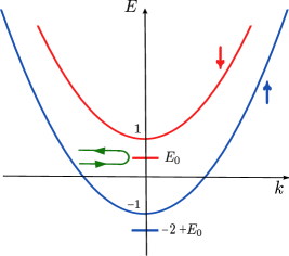
Figure 1: (Color online) Schematic illustration of the resonant reflection. An attractive impurity creates bound states under the bottoms of $\downarrow$ (red) and $\uparrow$ (blue) sub-bands. The binding energy, measured in the units of $\Delta$, is $1-E_{\scriptscriptstyle 0}$ Weak spin-orbit coupling mixes $\downarrow$ and $\uparrow$ wave functions. As a result, an incident $\uparrow$ electron undergoes a resonant scattering, illustrated by a green line. The result of the scattering is almost full reflection rather than conventional resonant transmission.

II Resonant reflection

In the presence of the Zeeman field and spin-orbit coupling, the Hamiltonian of a wire has the form

$$\hat{H}=\begin{pmatrix}-\frac{\hbar^{2}k_{x}^{2}}{2m}-\Delta&&i\gamma k_{x}\\ \\ -i\gamma k_{x}&&-\frac{\hbar^{2}k_{x}^{2}}{2m}+\Delta\end{pmatrix},$$ (1)

where $m$ is the electron mass, $2\Delta$ is the Zeeman splitting, and $\gamma$ is the spin-orbit coupling strength.

We assume that the impurity potential is short-ranged, $V(x)=V_{0}\delta(x)$. The system of coupled equations for $\uparrow$ and $\downarrow$ components of the spinor reads

$$-\frac{\hbar^{2}}{2m}\frac{\partial^{2}\psi_{1}}{\partial x^{2}}+V_{0}\delta(x)\psi_{1}-(\varepsilon+\Delta)\psi_{1}=\gamma\frac{\partial\psi_{2}}{\partial x},$$

$$-\frac{\hbar^{2}}{2m}\frac{\partial^{2}\psi_{2}}{\partial x^{2}}+V_{0}\delta(x)\psi_{2}-(\varepsilon-\Delta)\psi_{2}=-\gamma\frac{\partial\psi_{1}}{\partial x}.$$ (2)

Since the energy of the incident $\uparrow$ electron in resonance with impurity level of $\downarrow$ electron is close to $\Delta$, see Fig. 1, it is convenient to introduce the following dimensionless variables

$$z=\frac{x}{x_{0}},\hskip 28.45274ptE=\frac{\varepsilon}{\Delta},$$

$$\alpha=\left(\frac{2mx_{0}}{\hbar^{2}}\right)\gamma,~{}U_{0}=\left(\frac{2mx_{0}}{\hbar^{2}}\right)V_{0},$$ (3)

where the characteristic length,

$$x_{0}=\left(\frac{\hbar^{2}}{2m\Delta}\right)^{1/2},$$ (4)

is the de Broglie wave length of the electron with energy $\varepsilon=\Delta$. In the dimensionless variables the system Eq. (II) takes the form

$$-\frac{\partial^{2}\psi_{1}}{\partial z^{2}}+U_{0}\delta(z)\psi_{1}-(E+1)\psi_{1}=\alpha\frac{\partial\psi_{2}}{\partial z},$$

$$-\frac{\partial^{2}\psi_{2}}{\partial z^{2}}+U_{0}\delta(z)\psi_{2}-(E-1)\psi_{2}=-\alpha\frac{\partial\psi_{1}}{\partial z}.$$ (5)

Without impurity, the solutions of the system Eq. (II) in the domain $-1<E<1$ correspond to propagation of $\uparrow$ spin component and the decay of $\downarrow$ spin component, see Fig. 1. Due to spin-orbit coupling, both components of corresponding spinors are nonzero,

$$\begin{pmatrix}\psi_{1}\\ \\ \psi_{2}\end{pmatrix}=\begin{pmatrix}1\\ \\ iC\end{pmatrix}e^{iqz},~{}\begin{pmatrix}\psi_{1}\\ \\ \psi_{2}\end{pmatrix}=\begin{pmatrix}D\\ \\ 1\end{pmatrix}e^{-\kappa z},$$ (6)

where the wave vector, $q$, the decay constant, $\kappa$, and the components, $C$ and $D$, of the spinors are given by

$$q(E) = (1+E)^{1/2},~{}\kappa(E)=(1-E)^{1/2},$$

$$C = \frac{1}{2}\alpha q,~{}~{}~{}~{}D=\frac{1}{2}\alpha\kappa.$$ (7)

Coefficients $C$ and $D$ describe the admixture of the opposite spin projection due to spin-orbit coupling.

In the presence of impurity, the general solution at $z<0$ has a form

$$\begin{pmatrix}\psi_{1}\\ \\ \psi_{2}\end{pmatrix}=\begin{pmatrix}1\\ \\ iC\end{pmatrix}e^{iqz}+r_{1}\begin{pmatrix}1\\ \\ -iC\end{pmatrix}e^{-iqz}+r_{2}\begin{pmatrix}D\\ \\ 1\end{pmatrix}e^{\kappa z},$$ (8)

which is the combination of the solutions Eq. (6). First two terms describe the incident and the reflected $\uparrow$ waves, while the third term describes the solution corresponding to $\downarrow$, which decays at $z\rightarrow-\infty$.

The corresponding solution for $z>0$ reads

$$\begin{pmatrix}\psi_{1}\\ \\ \psi_{2}\end{pmatrix}=t_{1}\begin{pmatrix}1\\ \\ iC\end{pmatrix}e^{iqz}+t_{2}\begin{pmatrix}-D\\ \\ 1\end{pmatrix}e^{-\kappa z}.$$ (9)

The first term describes the transmitted $\uparrow$ wave, while the second term describes the decay of $\downarrow$ component.

Although the parameters $C$ and $D$ are proportional to $\alpha$, and thus are small due to the weakness of the spin-orbit coupling, it is these admixtures that are responsible for the resonant reflection. To capture this effect, we follow the standard procedure and calculate the reflection and transmission coefficients from the system of boundary conditions at $z=0$.

Continuity of the wave function Eqs. (8) and (9) yields two conditions

$$1+r_{1}+r_{2}D=t_{1}-t_{2}D,$$

$$iC(1-r_{1})+r_{2}=iCt_{1}+t_{2}.$$ (10)

The other two conditions come from the discontinuity of the derivatives, $\frac{\partial\psi_{1}}{\partial z}$ and $\frac{\partial\psi_{2}}{\partial z}$, at $z=0$. Integrating the system Eq. (II) near $z=0$, we get

$$iqt_{1}+\kappa t_{2}D-\Big{[}iq(1-r_{1})+\kappa r_{2}D\Big{]}=U_{0}(t_{1}-t_{2}D),$$

$$-qCt_{1}-\kappa t_{2}-\Big{[}-qC-qCr_{1}+\kappa r_{2}\Big{]}=U_{0}(iCt_{1}+t_{2}).\hskip 8.53581pt$$ (11)

Simplifying the above boundary conditions by introducing $R_{2}=Dr_{2}$, $T_{2}=Dt_{2}$, and $\lambda=CD$, we get

$$R_{2}+T_{2}=t_{1}-r_{1}-1,$$

$$R_{2}-T_{2}=i\lambda(t_{1}+r_{1}-1),$$ (12)

$$iq(t_{1}+r_{1})-U_{0}t_{1}-iq=R_{2}\kappa-(\kappa+U_{0})T_{2},$$

$$(\kappa+U_{0})T_{2}+\kappa R_{2}=-\lambda\Big{[}-it_{1}(iq-U_{0})-q(1+r_{1})\Big{]}.\hskip 8.53581pt$$ (13)

Since we are interested in the reflection and transmission coefficients, $r_{1}$ and $t_{1}$, it is convenient to express $R_{2}$ and $T_{2}$ from the system Eq. (II) and substitute them into the system Eq. (II), which assumes the form

$$t_{1}+r_{1}=\frac{\Big{[}q-\lambda(\kappa+\frac{U_{0}}{2})\Big{]}+i\frac{U_{0}}{2}}{\Big{[}q-\lambda(\kappa+\frac{U_{0}}{2})\Big{]}-i\frac{U_{0}}{2}},$$ (14)

$$t_{1}-r_{1}=\frac{\kappa+\frac{U_{0}}{2}+q\lambda-i\lambda\frac{U_{0}}{2}}{\kappa+\frac{U_{0}}{2}+q\lambda+i\lambda\frac{U_{0}}{2}}.$$ (15)

We see that the absolute values of $t_{1}+r_{1}$ and $t_{1}-r_{1}$ are equal to $1$. Then it is convenient to cast the solution of the system Eq. (14) into the form

$$|r_{1}|^{2}=\sin^{2}(\Phi_{-}-\Phi_{+}),~{}~{}|t_{1}|^{2}=\cos^{2}(\Phi_{-}-\Phi_{+}),$$ (16)

where

$$\Phi_{+}=\frac{1}{2}\tan^{-1}\frac{\frac{U_{0}}{2}}{q-\lambda(\kappa+\frac{U_{0}}{2})},$$

$$~{}\Phi_{-}=\frac{1}{2}\tan^{-1}\frac{\frac{\lambda U_{0}}{2}}{\kappa+\frac{U_{0}}{2}+q\lambda}.$$ (17)

Until now the calculation was exact. Weakness of spin-orbit coupling, quantified by the condition $\alpha\ll 1$, was used in the explicit expressions for $q$ and $\kappa$. We will now use this condition to simplify the phases $\Phi_{+}$ and $\Phi_{-}$. First, we note that the dimensionless parameter

$$\lambda=CD=\frac{1}{4}\alpha^{2}(1-E^{2})^{1/2}$$ (18)

is quadratic in spin-orbit coupling strength. This allows one to simplify $\Phi_{+}$ to $\tan^{-1}\left(\frac{U_{0}}{2q}\right)$. Then $\Phi_{+}$ can be identified with the scattering phase of $\uparrow$ electron from the impurity in the absence of spin-orbit coupling.

Turning to the phase $\Phi_{-}$, we note that the small parameter $\alpha^{2}$ in the expression for $\lambda$ allows one to neglect the term $q\lambda$ in the denominator. Then we see that, for attractive impurity, $U_{0}<0$, this denominator turns to zero at energy $E=E_{\scriptscriptstyle 0}$ determined by the condition

$$\kappa(E_{\scriptscriptstyle 0})=\frac{|U_{0}|}{2}.$$ (19)

This condition expresses the fact that in the absence of spin-orbit coupling, the energy position of the level of $\downarrow$ electron in the potential $U_{0}\delta(z)$ is $E=E_{\scriptscriptstyle 0}$, see Fig. 1.

To establish the energy width, $\Gamma$, of the resonance, we recast the expression for $\tan\Phi_{-}$ into the form

$$\tan\left[\Phi_{-}(E)\right]=\frac{1}{8}\alpha^{2}(1-E^{2})^{1/2}|U_{0}|\Bigg{[}\frac{(1-E^{2})^{1/2}+\frac{|U_{0}|}{2}}{1-E-\frac{U_{0}^{2}}{4}}\Bigg{]}.$$ (20)

Near the resonance, $E=E_{\scriptscriptstyle 0}=1-\frac{U_{0}^{2}}{4}$, the expression Eq. (20) assumes the conventional Breit-Wigner form

$$\tan\left[\Phi_{-}(E)\right]=\frac{\Gamma}{E_{\scriptscriptstyle 0}-E},$$ (21)

where $\Gamma$ is given by

$$\Gamma=\frac{\alpha^{2}}{16}|U_{0}|^{3}.$$ (22)

With binding energy of $\downarrow$ electron being $\frac{U_{0}^{2}}{4}$, we see that the width, $\Gamma$, is much smaller than this binding energy, which justifies the expansion near the resonance.

If the bound state in the potential $U_{0}\delta(z)$ is shallow, i.e. $U_{0}\ll 1$, we can replace $\tan^{-1}$ in expression for $\Phi_{+}$ by the argument. After that, the final expression for the energy-dependent reflection coefficient assumes the form

$$|r_{1}(E)|^{2} = \sin^{2}\left[\tan^{-1}\left(\frac{\Gamma}{E_{\scriptscriptstyle 0}-E}\right)-\frac{|U_{0}|}{2q}\right]$$ (23)

$$= \frac{\Big{[}\Gamma-\frac{|U_{0}|}{2q}(E_{\scriptscriptstyle 0}-E)\Big{]}^{2}}{(E_{\scriptscriptstyle 0}-E)^{2}+\Gamma^{2}}.$$

It follows from Eq. (23) that $|r_{1}(E)|^{2}$ has a characteristic Fano shapeFano . Near the resonance, $E=E_{\scriptscriptstyle 0}$, it is a Lorentzian with the width, $\Gamma$. As the energy is swept through $E_{\scriptscriptstyle 0}$, the reflection coefficient passes through zero (antiresonace) before returning to its non-resonant value $|r_{1}|^{2}=\frac{|U_{0}|^{2}}{4q^{2}}$.

III Incorporating the electron-electron interactions

As it was explained in the Introduction, the effect of interactions is more pronounced in the case of resonant reflection than in the case of resonant transmission.Nazarov2003 ; Gornyi2003 The reason is that the amplitude of the Friedel oscillations is proportional to the reflection amplitudeYue1993 ; Yue1994 which, for resonant reflection, is close to $1$. On the other hand, the Friedel oscillation of electron density creates perturbations which play the role of the “Bragg mirrors” for incident and transmitted electron waves. As a result of Friedel oscillations being strong, each Bragg mirror is highly “reflective”. This suggests to incorporate the effect of attenuation, caused by the mirrors, more accurately than in Refs. Nazarov2003, , Gornyi2003, .

The process of electron reflection from a compound object consisting of three scatterers, two Bragg mirrors and impurity between them, is illustrated in Fig. 2. The rigorous way to describe this reflection analytically is by employing the scattering matrices of each scatterer relating the amplitudes of the incoming and outgoing partial waves. These matrices are defined as follows

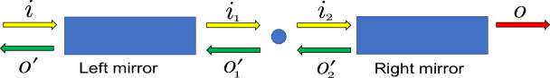
Figure 2: (Color online) Schematic illustration of the electron scattering from impurity “dressed” by Friedel oscillations, which play the role of the Bragg mirrors. The incident electron, $i$, can be reflected by the left mirror, by the impurity, or by the right mirror.

$$\begin{pmatrix}i_{1}\\ \\ o^{\prime}\end{pmatrix}=\begin{pmatrix}t_{L}&&r_{L}\\ \\ -r_{L}^{*}&&t_{L}^{*}\end{pmatrix}\begin{pmatrix}i\\ \\ o^{\prime}_{1}\end{pmatrix},~{}\begin{pmatrix}i_{2}\\ \\ o^{\prime}_{1}\end{pmatrix}=\begin{pmatrix}t_{1}&&r_{1}\\ \\ -r_{1}^{*}&&t_{1}^{*}\end{pmatrix}\begin{pmatrix}i_{1}\\ \\ o^{\prime}_{2}\end{pmatrix},~{}~{}\begin{pmatrix}o\\ \\ o^{\prime}_{2}\end{pmatrix}=\begin{pmatrix}t_{R}&&r_{R}\\ \\ -r_{R}^{*}&&t_{R}^{*}\end{pmatrix}\begin{pmatrix}i_{2}\\ \\ 0\end{pmatrix}.$$ (24)

The amplitude $r_{1}$ in Eq. (24) was found in the previous section. Two remaining amplitudes, $r_{L}$ and $r_{R}$, will be calculated later. Excluding the intermediate amplitudes, $i_{1}$, $i_{2}$, $o_{1}^{\prime}$, $o_{2}^{\prime}$ from Eq. (24), we find the expression for the net amplitude reflection coefficient of the compound scatterer

$$r_{\scriptscriptstyle eff}=-\frac{o^{\prime}}{i}=\frac{r_{L}^{*}+r_{1}^{*}+r_{R}^{*}+r_{L}^{*}r_{1}r_{R}^{*}}{1+r_{1}r_{R}^{*}+r_{L}r_{1}^{*}+r_{L}r_{R}^{*}}.$$ (25)

To analyze this expression, we express the power reflection coefficient, $|r_{\scriptscriptstyle eff}|^{2}$, via the magnitudes of the reflection coefficients $r_{1}$, $r_{L}$, and $r_{R}$ and obtain

$$|r_{\scriptscriptstyle eff}|^{2}=1-|t_{\scriptscriptstyle eff}|^{2}=1-\frac{\left(1-|r_{\textit{\tiny{Bragg}}}|^{2}\right)^{2}\left(1-|r_{1}|^{2}\right)}{\Big{(}1+|r_{\textit{\tiny{Bragg}}}|^{2}+2|r_{\textit{\tiny{Bragg}}}||r_{1}|\cos\beta\Big{)}^{2}}.$$ (26)

In Eq. (26) we took into account that, unlike Refs. Nazarov2003, , Gornyi2003, , there is a symmetry between the left and right mirrors, so that the magnitudes, $|r_{L}|$ and $|r_{R}|$ are equal to each other and are denoted with $|r_{\textit{\tiny{Bragg}}}|$. The phase, $\beta$, is the combination of the phase $\Phi_{-}$, defined by Eq. (16), and the phase, $\Phi_{\textit{\tiny{Bragg}}}$, accumulated in the course of the reflection from the mirror. We will see that this phase is big and depends strongly on the energy. Thus, we average Eq. (26) over $\beta$ using the identity

$$\Bigg{\langle}\frac{1}{(a+\cos\beta)^{2}}\Bigg{\rangle}_{\beta}=\frac{a}{(a^{2}-1)^{3/2}}.$$ (27)

The result of this averaging reads

$$\langle|r_{\scriptscriptstyle eff}|^{2}\rangle=1-\frac{\left(1-|r_{\textit{\tiny{Bragg}}}|^{2}\right)^{2}\left(1+|r_{\textit{\tiny{Bragg}}}|^{2}\right)\left(1-|r_{1}|^{2}\right)}{\Big{[}\left(1-|r_{\textit{\tiny{Bragg}}}|^{2}\right)^{2}+4|r_{\textit{\tiny{Bragg}}}|^{2}\left(1-|r_{1}|^{2}\right)\Big{]}^{3/2}}.$$ (28)

It is also instructive to express the effective power transmission coefficient via the partial transmission coefficients $|t_{1}|^{2}$ and $|t_{\textit{\tiny{Bragg}}}|^{2}$. One obtains

$$\langle|t_{\scriptscriptstyle eff}|^{2}\rangle=\frac{|t_{\textit{\tiny{Bragg}}}|^{4}\left(2-|t_{\textit{\tiny{Bragg}}}|^{2}\right)|t_{1}|^{2}}{\Big{[}|t_{\textit{\tiny{Bragg}}}|^{4}+4\left(1-|t_{\textit{\tiny{Bragg}}}|^{2}\right)|t_{1}|^{2}\Big{]}^{3/2}}.$$ (29)

Since the transmission, $|t_{\textit{\tiny{Bragg}}}|^{2}$, is strongly dependent on the position of the Fermi level, $E_{\scriptscriptstyle F}$, with respect to the resonant energy level, $E_{\scriptscriptstyle 0}$, the magnitude of $|t_{\textit{\tiny{Bragg}}}|^{2}$ falls off with increasing $(E_{\scriptscriptstyle F}-E_{\scriptscriptstyle 0})$. Then one would expect that $|t_{\scriptscriptstyle eff}|^{2}$ grows monotonically with increasing $|t_{\textit{\tiny{Bragg}}}|^{2}$ and approaches $|t_{1}|^{2}$. The reasoning behind this expectation is that the scattering by the Bragg mirrors becomes inefficient for large $(E_{\scriptscriptstyle F}-E_{\scriptscriptstyle 0})$. Remarkably, the dependence of $|t_{\scriptscriptstyle eff}|^{2}$, described by Eq. (29), is non-monotonic. As illustrated in Fig. 3, this dependence has a maximum. For small transmission of the impurity, $|t_{1}|^{2}\ll 1$, the position of maximum is easy to calculate analytically. It is $|t_{\textit{\tiny{Bragg}}}|^{4}=8t_{1}^{2}$. Note that the value $|t_{\textit{\tiny{Bragg}}}|^{4}$ has a meaning of the net transmission of two mirrors. Thus, the maximum occurs when the transmissions of the impurity and of the two mirrors are equal within numerical factor. Substituting $|t_{\textit{\tiny{Bragg}}}|^{4}=8t_{1}^{2}$ into Eq. (29), we find the maximal value of the effective power transmission

$$\left(|t_{\scriptscriptstyle eff}|^{2}\right)_{\scriptscriptstyle max}=\frac{2}{3^{3/2}}|t_{1}|.$$ (30)

We see that this value is much bigger than $|t_{1}|^{2}$.

The origin of the maximum is that the dominant contribution to the phase-averaged transmission, $\langle|t_{\scriptscriptstyle eff}|^{2}\rangle$, comes from the phases, $\beta$, in Eq. (26) for which the denominator is close to zero. In other words, while the impurity alone acts as a reflector, adding of the two Bragg mirrors can lead to the resonant transmission.

Naturally, the values of $|t_{1}|^{2}$ and $|t_{\textit{\tiny{Bragg}}}|^{2}$ are not independent. It is the reflection from the impurity that controls the magnitude of the Friedel oscillations. To analyze the behavior the effective transmission with energy, $E$, of the incident electron and with $E_{\scriptscriptstyle F}$, we need to specify the analytical form of $|t_{\textit{\tiny{Bragg}}}|^{2}$. This is done in the next section.

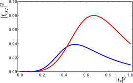
Figure 3: (Color online) Effective power transmission coefficient of the impurity dressed by the Friedel oscillations is plotted from Eq. (29) versus the transmission of the Bragg mirrors for $|t_{1}|^{2}=0.01$ (blue) and $|t_{1}|^{2}=0.04$ (red).

IV Transmission of the Bragg mirror

In the presence of electron-electron interactions, propagation of electron through the mirror is described by the Schrödinger equation

$$-\frac{\partial^{2}\psi_{1}}{\partial z^{2}}+V_{H}(z)\psi_{1}+\hat{V}_{ex}\Big{\{}\psi_{1}\Big{\}}=\left(E+1\right)\psi_{1},$$ (31)

where $V_{H}(z)$ and $\hat{V}_{ex}$ are the Hartree and the exchange terms, respectively. When the interaction is short-ranged, one can consider only the Hartree term, since the exchange term causes only a modification of the interaction constant.Yue1993 The other consequence of the interaction being short-ranged is that the Hartree potential is proportional to the modulation of the electron density created by the Friedel oscillationsYue1993 , i.e. it has the from

$$V_{H}(z)=\frac{\mu(E_{\scriptscriptstyle F})}{q_{\scriptscriptstyle F}|z|}\cos(2q_{\scriptscriptstyle F}|z|),$$ (32)

where $q_{\scriptscriptstyle F}$ is the Fermi momentum. The magnitude of the electron-electron interactions as well as the energy dependence of $|r_{1}|$, responsible for the Friedel oscillations, are encoded into the constant, $\mu$, which we will specify later. The main difference between our approach and the approach of Ref. Yue1993, is that we find an asymptotically exact solution of Eq. (31), while in Ref. Yue1993, it was solved perturbatively. The reason why asymptotically exact solution can be found is that the amplitude of $V_{H}(z)$ falls off slowly with $z$, so that the relevant values of $q_{\scriptscriptstyle F}z$ are big. This, in turn, suggests to search for $\psi_{1}(z)$ in the form

$$\psi_{1}(z)=A_{+}(z)e^{iq_{\scriptscriptstyle F}z}+A_{-}(z)e^{-iq_{\scriptscriptstyle F}z},$$ (33)

where the functions $A_{+}$ and $A_{-}$ change slowly with $z$, so that their second derivatives can be neglected. Upon substituting Eq. (33) into Eq. (31), and neglecting non-resonant terms $\exp(\pm 3iq_{\scriptscriptstyle F}z)$, we arrive to a coupled system of the first-order equations

$$-2iq_{\scriptscriptstyle F}\frac{\partial A_{+}(z)}{\partial z}+\frac{\mu}{2z}A_{-}(z)=\left(E+1-q_{\scriptscriptstyle F}^{2}\right)A_{+}(z),$$

$$2iq_{\scriptscriptstyle F}\frac{\partial A_{-}(z)}{\partial z}+\frac{\mu}{2z}A_{+}(z)=\left(E+1-q_{\scriptscriptstyle F}^{2}\right)A_{-}(z).\hskip 5.69054pt$$ (34)

It appears that this system can be solved exactly for arbitrary interaction strength, $\mu$. To see this, we first perform a rescaling

$$y=z\left(\frac{E+1-q_{\scriptscriptstyle F}^{2}}{2q_{\scriptscriptstyle F}}\right),$$ (35)

and then introduce the auxiliary functions

$$a(y)=A_{+}(y)+iA_{-}(y),~{}b(y)=A_{+}(y)-iA_{-}(y).$$ (36)

Then the system Eq. (IV) reduces to

$$\frac{\partial a}{\partial y}+\frac{\mu}{4q_{\scriptscriptstyle F}y}a(y)=ib(y),$$

$$\frac{\partial b}{\partial y}-\frac{\mu}{4q_{\scriptscriptstyle F}y}b(y)=ia(y).$$ (37)

In the rescaled form, the system contains a single dimensionless parameter, $\frac{\mu}{4q_{\scriptscriptstyle F}}$. As a next step, we substitute $b(y)$ from the first equation into the second equation and arrive to the following second-order differential equation

$$\frac{\partial^{2}a}{\partial y^{2}}+\Bigg{[}1+\frac{1-4(\frac{\mu}{4q_{\scriptscriptstyle F}}+\frac{1}{2})^{2}}{4y^{2}}\Bigg{]}a(y)=0.$$ (38)

The general solution of this equation can be presented as a linear combination

$$a(y)=y^{1/2}\Big{[}c_{\scriptscriptstyle 1}J_{\scriptscriptstyle\frac{\mu}{4q_{\scriptscriptstyle F}}+\frac{1}{2}}(y)+c_{\scriptscriptstyle 2}J_{\scriptscriptstyle-\frac{\mu}{4q_{\scriptscriptstyle F}}-\frac{1}{2}}(y)\Big{]},$$ (39)

where $J_{\scriptscriptstyle\frac{\mu}{4q_{\scriptscriptstyle F}}+\frac{1}{2}}$ and $J_{\scriptscriptstyle-\frac{\mu}{4q_{\scriptscriptstyle F}}-\frac{1}{2}}$ are the Bessel functions. At large $y$ both Bessel functions oscillate, so that the value of the transmission coefficient is governed by the ratio $c_{\scriptscriptstyle 1}/c_{\scriptscriptstyle 2}$. This ratio is determined by the condition that at small $y=y_{c}$, where the Friedel oscillations are terminated (see Appendix A), the amplitude of the reflected wave vanishes. The final expression for the transmission coefficient, reads

$$t_{\textit{\tiny{Bragg}}}=\frac{\left(2\pi y_{c}\right)^{1/2}J_{\scriptscriptstyle\frac{\mu}{4q_{\scriptscriptstyle F}}-\frac{1}{2}}(y_{c})J_{\scriptscriptstyle-\frac{\mu}{4q_{\scriptscriptstyle F}}-\frac{1}{2}}(y_{c})}{J_{\scriptscriptstyle\frac{\mu}{4q_{\scriptscriptstyle F}}-\frac{1}{2}}(y_{c})e^{i\frac{\pi\mu}{8q_{\scriptscriptstyle F}}}+J_{\scriptscriptstyle-\frac{\mu}{4q_{\scriptscriptstyle F}}-\frac{1}{2}}(y_{c})e^{-i\frac{\pi\mu}{8q_{\scriptscriptstyle F}}}}.$$ (40)

The details of the derivation are presented in the Appendix B.

The result Eq. (40) can be simplified when $y_{c}$ is small. Then we can use the small-argument asymptotes of the Bessel functions and obtain

$$t_{\textit{\tiny{Bragg}}}=\frac{1}{\cosh\left(\frac{\mu}{4q_{\scriptscriptstyle F}}\ln y_{c}\right)}.$$ (41)

In deriving this expression we took into account that the interactions are weak in the usual sense, namely that the typical interaction energy is much smaller than the Fermi energy. This condition ensures that $\frac{\mu}{q_{\scriptscriptstyle F}}$ is small.

Concerning the value of $y_{c}$, in Appendix A it is demonstrated that the Friedel oscillations are terminated at $z=z_{c}\sim\frac{q_{\scriptscriptstyle 0}}{\Gamma}$. Using the relation Eq. (35), we find that, within a numerical factor, $y_{c}$ is given by

$$y_{c}=\frac{E-E_{\scriptscriptstyle F}}{\Gamma}.$$ (42)

We see that in the interesting limit when the Fermi level is close to the resonance $y_{c}$ is indeed small.

Equations (41) and (42) describe how the transmission of the Bragg mirror evolves with energy. Indeed, the argument of the hyperbolic cosine is the product of a small factor $\frac{\mu}{4q_{\scriptscriptstyle F}}$ and a big factor $\ln y_{c}$. If this product is small, e.g. when the interactions are weak, then the transmission coefficient is close to $1$. On the contrary, if the product is big, we have

$$t_{\textit{\tiny{Bragg}}}=\left(\frac{2|E-E_{\scriptscriptstyle F}|}{\Gamma}\right)^{\frac{|\mu|}{4q_{\scriptscriptstyle F}}}\ll 1,$$ (43)

i.e. the mirror is highly reflective.

To conclude this Section, we present the microscopic expression for the parameter $\mu$ in terms of the Fourier components of the interaction potential. This expression follows from the expression for the amplitude of the oscillations of the electron density, calculated in Appendix A, and has the form

$$\mu=\frac{\nu q_{\scriptscriptstyle F}}{2}|r_{1}(E_{\scriptscriptstyle F})|^{2},$$ (44)

where $\nu$ is given by

$$\nu=\frac{V(0)-V(2q_{\scriptscriptstyle F})}{2\pi\hbar v_{\scriptscriptstyle F}}.$$ (45)

The term $V(0)$ comes from the exchange potential, while $V(2q_{\scriptscriptstyle F})$ comes from the Hartree potential; $v_{\scriptscriptstyle F}$ stands for the Fermi velocity.

Note that the transmission, $t_{\textit{\tiny{Bragg}}}$, is full not only in the absence of electron-electron interactions. If the interactions are present, but there is no reflection from the impurity, $r_{1}(E_{\scriptscriptstyle F})=0$, then transmission is also full. This is natural, since in the absence of reflection, the Friedel oscillations do not form.

V Energy dependence of the effective reflection

In Eq. (29) both $t_{1}$ and $t_{\textit{\tiny{Bragg}}}$ are the functions of energy. While $t_{1}$ is a growing function of energy, $t_{\textit{\tiny{Bragg}}}$ grows with increasing $|E-E_{\scriptscriptstyle F}|$. In addition, the power, $\frac{\mu}{4q_{\scriptscriptstyle F}}$, in Eq. (43) depends on the difference $|E_{\scriptscriptstyle 0}-E_{\scriptscriptstyle F}|$, see Appendix A.

Concerning the overall dependence $|r_{\scriptscriptstyle eff}(E)|^{2}$, the situation is most transparent when the Fermi level lies away from the resonance. Then the presence of the Bragg mirrors manifests itself only near $E=E{\scriptscriptstyle F}$. Bragg mirrors cause a spike in the reflection. When the spacing between $E_{\scriptscriptstyle F}$ and $E_{\scriptscriptstyle 0}$ is much smaller than the width of the resonance, there are two features in $|r_{\scriptscriptstyle eff}(E)|^{2}$-dependence that are present for any interaction strength. Firstly, the reflection is full for any position of the Fermi level when the energy of the incident electron is $E=E_{\scriptscriptstyle 0}$. This is because the electron is fully reflected even in the absence of the Friedel oscillations. Secondly, $|r_{\scriptscriptstyle eff}(E)|^{2}=1$ at $E=E_{\scriptscriptstyle F}$ due to full reflection from the mirror. Thus, in the domain $-E_{\scriptscriptstyle F}<E<0$, the reflection coefficient should pass through a minimum. Indeed, this minimum is present in the curves $|r_{\scriptscriptstyle eff}(E)|^{2}$ plotted from Eqs. (28) and (41) in Fig. 4.

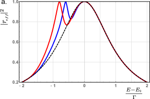
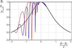
Figure 4: (Color online) (a) In the absence of interactions, the effective power reflection coefficient is a Lorentzian, $|r_{\scriptscriptstyle eff}|^{2}=\left[1+\frac{(E-E_{\scriptscriptstyle 0})^{2}}{\Gamma^{2}}\right]^{-1}$ (black dashed line). With interactions, full reflection takes place at two energies $E=E_{\scriptscriptstyle 0}$ as a result of scattering from the impurity and at $E=E_{\scriptscriptstyle F}$ as a result of scattering from the Bragg mirror. This is illustrated by red and blue curves plotted from Eqs. (28) and (41) for $(E_{\scriptscriptstyle 0}-E_{\scriptscriptstyle F})=0.8\Gamma$ and $(E_{\scriptscriptstyle 0}-E_{\scriptscriptstyle F})=0.6\Gamma$, respectively. The interaction strength in both curves is chosen to be $\frac{\mu}{4q_{\scriptscriptstyle F}}=0.4$. (b) Scattering by two Bragg mirrors can, for certain energies, transform the resonant reflection into the resonant transmission. While the plot (a) shows the average over the phase, $\beta$, the plot (b) shows the reflection profile for the same parameters prior to averaging.

VI Discussion

(i) To establish the relation between our results and those obtained within the renormalization-group approachYue1993 ; Yue1994 ; Maslov ; Nagaev ; Nazarov2003 ; Gornyi2003 we assume that the reflection of the Bragg mirrors is weak and expand Eq. (26) with respect to $|r_{\textit{\tiny{Bragg}}}|^{2}$. This yields

$$|r_{\scriptscriptstyle eff}|^{2}-|r_{1}|^{2}=4\left(1-|r_{1}|^{2}\right)\Big{[}|r_{\textit{\tiny{Bragg}}}|^{2}+|r_{1}||r_{\textit{\tiny{Bragg}}}|\cos\beta\Big{]}.$$ (46)

The second term in the brackets contains the first power of $|r_{\textit{\tiny{Bragg}}}|$, unlike the first term which contains $|r_{\textit{\tiny{Bragg}}}|^{2}$. This second term comes from interference of incident and reflected waves passing through the Bragg mirror. If we average Eq. (46) over $\beta$, the second term will disappear. Then it is the first term, $1-t_{\textit{\tiny{Bragg}}}^{2}$, that will describe the reduction of the transmission of the impurity due to electron-electron interactions. As follows from Eq. 41, $|r_{\textit{\tiny{Bragg}}}|^{2}$ is proportional to $|r_{1}|^{2}$ and contains $\mu\ln y_{c}$. Then Eq. (46) reproduces the main result of Ref. Yue1993, . In Ref. Yue1993, this result is subsequently converted to the renormalization-group equation. We studied the limit in which both $|r_{1}|$ and $|r_{\textit{\tiny{Bragg}}}|$ are close to $1$. Then the denominator in Eq. (26) is close to zero when $\cos\beta=-1$. Definitely, the expansion with respect to $|r_{\textit{\tiny{Bragg}}}|$ and subsequent summation of the leading terms, which is the essence of the renormalization-group approach, does not capture this resonant transmission.

(ii) Adopting of the renormalization group approach in Refs. Yue1993, ; Yue1994, ; Maslov, ; Nagaev, ; Nazarov2003, ; Gornyi2003, relies on the assumption that the coefficients of the expansion of $|t_{\scriptscriptstyle eff}|^{2}$ is powers of $\ln(|E-E_{\scriptscriptstyle F}|)$ fall off as $\frac{1}{n!}$. Our calculation is equivalent to the summation of all the orders of the expansion and confirms this assumption.

(iii) The form Eq. (23) of the resonant reflection is the same as for the resonant tunneling between the two electrodes via a localized state located between the electrons. This suggests the interpretation of the resonant transmission as resonant tunneling between left-moving and right-moving electrons. If this interpretation is correct, the width, $\Gamma$, calculated from the golden rule should coincide with Eq. (22), and, in particular, should be proportional to $U_{0}^{3}$. Taking into account that the normalized wave function of the localized state has the form $\psi_{2}(z)=\kappa^{1/2}\exp(-\kappa|z|)$, the matrix element of $\alpha\frac{\partial}{\partial z}$ between $\psi_{2}(z)$ and the right-moving plane wave, $\exp(iqz)$, is given by

$$i\alpha\kappa^{1/2}q\int\limits_{-\infty}^{\infty}dz\exp\Big{[}iqz-\kappa|z|\Big{]}=2i\frac{q\kappa^{3/2}}{q^{2}+\kappa^{2}}.$$ (47)

One can neglect $\kappa^{2}$ in the denominator. Then the square of the matrix element is proportional to $\kappa^{3}$ and thus to $U_{0}^{3}$, since, at resonance, $\kappa=\frac{U_{0}}{2}$.

(iv) There is a question whether the attenuation of electron wave functions upon passage of the Bragg mirrors disturbs the shape of the Friedel oscillations. It is important that this disturbance is negligible. Qualitatively, this follows from the fact that many states with $E<E_{\scriptscriptstyle F}$ are responsible for the formation of the Bragg mirrors, while only the states with $|E-E_{\scriptscriptstyle F}|\lesssim\nu\Gamma$ are strongly affected by the Bragg mirrors.

(v) Another question is why we did not take into account the Friedel oscillations originating from the electron reflection within the same sub-band. Indeed, while the Friedel oscillations caused by the resonant reflection develop at large distances $z_{c}\sim\frac{q_{0}}{\Gamma}$, “non-resonant” Friedel oscillations start at much smaller $z\sim 1$. To answer this question one should estimate the contribution to the reflection coefficient within the domain $1<z<z_{c}$, where non-resonant Friedel oscillations dominate. The amplitude of the these oscillations is $\sim\frac{U_{0}}{q_{\scriptscriptstyle F}}$ and they fall off as $1/z$. This leads to the estimate $\frac{U_{0}}{q_{\scriptscriptstyle F}}\ln(z_{c})$ as in Ref. Yue1993, . Since $\frac{U_{0}}{q_{\scriptscriptstyle F}}\ll 1$, the weakness of non-resonant reflection cannot be compensated by the logarithmically big factor $\ln\left(\frac{q_{0}}{\Gamma}\right)$, it is for this reason we have neglected the Friedel oscillations originating from the reflection within the same sub-band.

(vi) Our main finding is that, for weak transmission through a single Bragg mirror, the net transmission from two Bragg mirrors and the impurity can be close to one. This enhancement of the net transmission takes place when the “Fabry-Perot” condition $\cos\beta\approx-1$ is met. Then the denominator in Eq. (26) becomes small. This happens near certain distinct energies of incident electron. Averaging over the phase, $\beta$, employed above, requires that there are many such energies within the interval $|E_{0}-E_{\scriptscriptstyle F}|$. To verify that this is the case, consider the contribution to $\beta$ coming from the factor $\exp(iq_{\scriptscriptstyle F}z)$ in Eq. (33). As an estimate for $z$ in this factor one should take the effective length of the Bragg mirror where the reflection is formed. From Eq. (38) we see that this length is determined by the condition $y\gg 1$. At these values of $y$ the product $y^{1/2}J_{\scriptscriptstyle\frac{\mu}{4q_{\scriptscriptstyle F}}+\frac{1}{2}}(y)$ saturates meaning that the formation of the Bragg reflection is complete. The condition $y\gg 1$ transforms into the condition $z\gtrsim\frac{q_{\scriptscriptstyle F}}{E-E_{\scriptscriptstyle F}}$. Thus, the contribution to $\beta$ from the phase, $\Phi_{\textit{\tiny{Bragg}}}$, accumulation in the course of traveling through the mirror is of the order of $(E-E_{\scriptscriptstyle F})^{-1}$. In the relevant domain $|E_{0}-E_{\scriptscriptstyle F}|\lesssim\Gamma$ this phase goes through $(2n+1)\pi$ many times.

Acknowledgements

We are strongly grateful to E. G. Mishchenko for a number of illuminating discussions. The work was supported by the Department of Energy, Office of Basic Energy Sciences, Grant No. DE- FG02-06ER46313.

Appendix A Magnitude of the Friedel Oscillations

The scattering of electrons from the impurity modifies the electron densities around the impurity. In the presence of electron-electron interaction this modulation of density leads to an additional scattering, which we call “Bragg mirror” in the main text. This scattering barrier is also called Hartree potential,

$$V_{H}(z)=\int\limits_{-\infty}^{\infty}V(z-y)\delta n(y)dy,$$ (48)

where $V(z-y)$ is the interaction potential and $\delta n(y)$ is the fluctuation of the density. Assuming interaction to be short ranged, $V(z-y)=\nu~{}\delta(z-y)$, we see that the Hartree potential takes the form, $V_{H}(z)=\nu~{}\delta n(z)$. Now, the modulation of the electron density, $\delta n(z)$, which depends on the reflection coefficient, $r_{1}$, reads

$$\delta n(z)=\int\limits_{0}^{q_{\scriptscriptstyle F}}\frac{dq}{\pi}~{}2\text{Re}(r_{1}(q)~{}e^{2iqz})\\ =\int\limits_{0}^{q_{\scriptscriptstyle F}}\frac{dq}{\pi}\frac{\Gamma}{\left[\Gamma^{2}+\left(q_{\scriptscriptstyle 0}^{2}-q^{2}\right)^{2}\right]^{1/2}}\cos\left(2q|z|+\tan^{-1}\frac{\Gamma}{q_{\scriptscriptstyle 0}^{2}-q^{2}}\right),$$ (49)

where $q_{\scriptscriptstyle 0}=(1+E_{\scriptscriptstyle 0})^{1/2}$, see Eq. (II). Upon measuring $q$ from $q_{\scriptscriptstyle F}$ and introducing new variables,

$$u=2q_{\scriptscriptstyle 0}\frac{q_{\scriptscriptstyle F}-q}{\Gamma},~{}~{}u_{\scriptscriptstyle 0}=2q_{\scriptscriptstyle 0}\frac{q_{\scriptscriptstyle 0}-q_{\scriptscriptstyle F}}{\Gamma},$$ (50)

Eq. (49) assumes the form

$$\delta n(z)=\frac{\Gamma}{2\pi q_{\scriptscriptstyle 0}}\int\limits_{0}^{\frac{2q_{\scriptscriptstyle\scriptscriptstyle 0}q_{\scriptscriptstyle F}}{\Gamma}}du~{}\frac{1}{\Big{[}1+\left(u+u_{\scriptscriptstyle 0}\right)^{2}\Big{]}^{1/2}}\\ \times\cos\Bigg{[}2|z|\left(q_{\scriptscriptstyle F}-\frac{\Gamma}{2q_{\scriptscriptstyle 0}}u+\tan^{-1}\frac{1}{u+u_{\scriptscriptstyle 0}}\right)\Bigg{]}.$$ (51)

It is convenient to separate the contributions proportional to $\sin(2q|z|)$ and to $\cos(2q|z|)$. This yields

$$\delta n(z)=\frac{\Gamma}{2\pi q_{\scriptscriptstyle 0}}\int\limits_{0}^{\frac{2q_{\scriptscriptstyle\scriptscriptstyle 0}q_{\scriptscriptstyle F}}{\Gamma}}du~{}\frac{1}{1+\left(u+u_{\scriptscriptstyle 0}\right)^{2}}\times\\ \Bigg{\{}\left(u+u_{\scriptscriptstyle 0}\right)\cos\!\left[2|z|\left(q_{\scriptscriptstyle F}-\frac{\Gamma}{2q_{\scriptscriptstyle 0}}u\right)\right]-\sin\!\left[2|z|\left(q_{\scriptscriptstyle F}-\frac{\Gamma}{2q_{\scriptscriptstyle 0}}u\right)\right]\Bigg{\}}.$$ (52)

The shift, $\frac{\Gamma}{2q_{\scriptscriptstyle 0}}u$, of the arguments of both cosine and sine leads to the factors $\sin\left(\frac{\Gamma|z|}{q_{\scriptscriptstyle 0}}u\right)$ and $\cos\left(\frac{\Gamma|z|}{q_{\scriptscriptstyle 0}}u\right)$ in the numerator. For $\frac{\Gamma|z|}{q_{\scriptscriptstyle 0}}\gg 1$, both terms rapidly oscillate with $u$. Without $u$-dependence of the prefactor, the contribution from the cosine term will vanish. With the prefactor the contribution of this term remains much smaller than the contribution of the sine term. Retaining only the sine-term we get

$$\delta n(z)=\cos\left(2q_{\scriptscriptstyle F}|z|\right)\frac{\Gamma}{2\pi q_{\scriptscriptstyle 0}}\int\limits_{0}^{\frac{2q_{\scriptscriptstyle 0}q_{\scriptscriptstyle F}}{\Gamma}}du~{}\frac{\sin\left(\frac{\Gamma|z|}{q_{\scriptscriptstyle 0}}u\right)}{1+\left(u+u_{\scriptscriptstyle 0}\right)^{2}}.$$ (53)

For $\frac{\Gamma|z|}{q_{\scriptscriptstyle 0}}\gg 1$ we can replace the upper limit of the integral by infinity and neglect the $u$-dependence of the denominator. This leads to the final answer

$$\delta n(z)=\frac{|r_{1}(E_{\scriptscriptstyle F})|^{2}}{2\pi|z|}\cos\left(2q_{\scriptscriptstyle F}|z|\right),$$ (54)

where we have used the fact that $|r_{1}(E_{\scriptscriptstyle F})|^{2}$ is $(1+u_{\scriptscriptstyle 0}^{2})^{-1}$. Note that, unlike the conventional Friedel oscillationsYue1993 , Eq. (54) contains the second power of $|r_{1}(E_{\scriptscriptstyle F}|$. Extra power originates from the phase of the cosine in Eq. (51), which is strongly energy-dependent.

The most important outcome of the above analysis is that the Friedel oscillations are terminated at rather large distances $z=z_{c}\sim\frac{q_{\scriptscriptstyle 0}}{\Gamma}$. We have used this value as a cutoff of log-divergence in the main text.

Appendix B Calculation of transmission coefficient from more rigorous approach

Substituting the general form Eq. (39) of $a(y)$ in the system Eq. (IV) we find the following general form of $b(y)$

$$b(y)=-iy^{1/2}\Big{[}c_{\scriptscriptstyle 1}J_{\scriptscriptstyle\frac{\mu}{4q_{\scriptscriptstyle F}}-\frac{1}{2}}(y)-c_{\scriptscriptstyle 2}J_{\scriptscriptstyle-\frac{\mu}{4q_{\scriptscriptstyle F}}+\frac{1}{2}}(y)\Big{]}.$$ (55)

Once $a(y)$ and $b(y)$ are known, the incident amplitude, $A_{+}(y)=\frac{1}{2}[a(y)+b(y)]$, and the reflected amplitude $A_{-}(y)=\frac{1}{2i}[a(y)-b(y)]$ can be expressed as a combination of the Bessel functions

$$A_{+}=\frac{y^{1/2}}{2}\Bigg{\{}c_{\scriptscriptstyle 1}\Big{[}J_{\scriptscriptstyle\frac{\mu}{4q_{\scriptscriptstyle F}}+\frac{1}{2}}(y)-iJ_{\scriptscriptstyle\frac{\mu}{4q_{\scriptscriptstyle F}}-\frac{1}{2}}(y)\Big{]}$$

$$+c_{\scriptscriptstyle 2}\Big{[}J_{\scriptscriptstyle-\frac{\mu}{4q_{\scriptscriptstyle F}}-\frac{1}{2}}(y)+iJ_{\scriptscriptstyle-\frac{\mu}{4q_{\scriptscriptstyle F}}+\frac{1}{2}}(y)\Big{]}\Bigg{\}},$$ (56)

$$A_{-}=\frac{y^{1/2}}{2i}\Bigg{\{}c_{\scriptscriptstyle 1}\Big{[}J_{\scriptscriptstyle\frac{\mu}{4q_{\scriptscriptstyle F}}+\frac{1}{2}}(y)+iJ_{\scriptscriptstyle\frac{\mu}{4q_{\scriptscriptstyle F}}-\frac{1}{2}}(y)\Big{]}$$

$$+c_{\scriptscriptstyle 2}\Big{[}J_{\scriptscriptstyle-\frac{\mu}{4q_{\scriptscriptstyle F}}-\frac{1}{2}}(y)-iJ_{\scriptscriptstyle-\frac{\mu}{4q_{\scriptscriptstyle F}}+\frac{1}{2}}(y)\Big{]}\Bigg{\}}.$$ (57)

In the limit $y\rightarrow\infty$, the behavior of $A_{+}$ and $A_{-}$ is the following

$$A_{+}=\frac{1}{(2\pi)^{1/2}}\Big{[}c_{\scriptscriptstyle 2}e^{i\frac{\pi\mu}{8q_{\scriptscriptstyle F}}}-ic_{\scriptscriptstyle 1}e^{-i\frac{\pi\mu}{8q_{\scriptscriptstyle F}}}\Big{]}e^{iy},$$

$$A_{-}=\frac{-i}{(2\pi)^{1/2}}\Big{[}c_{\scriptscriptstyle 2}e^{-i\frac{\pi\mu}{8q_{\scriptscriptstyle F}}}+ic_{\scriptscriptstyle 1}e^{i\frac{\pi\mu}{8q_{\scriptscriptstyle F}}}\Big{]}e^{-iy}.$$ (58)

For small $y$, we have $J_{\scriptscriptstyle\pm\frac{\mu}{4q_{\scriptscriptstyle F}}+\frac{1}{2}}(y)\ll J_{\scriptscriptstyle\pm\frac{\mu}{4q_{\scriptscriptstyle F}}-\frac{1}{2}}(y)$, so the asymptotic expressions for $A_{+}$ and $A_{-}$ can be written as

$$A_{-}=\frac{y^{1/2}}{2i}\Big{[}ic_{\scriptscriptstyle 1}J_{\scriptscriptstyle\frac{\mu}{4q_{\scriptscriptstyle F}}-\frac{1}{2}}(y)+c_{\scriptscriptstyle 2}J_{\scriptscriptstyle-\frac{\mu}{4q_{\scriptscriptstyle F}}-\frac{1}{2}}(y)\Big{]},$$

$$A_{+}=\frac{y^{1/2}}{2}\Big{[}-ic_{\scriptscriptstyle 1}J_{\scriptscriptstyle\frac{\mu}{4q_{\scriptscriptstyle F}}-\frac{1}{2}}(y)+c_{\scriptscriptstyle 2}J_{\scriptscriptstyle-\frac{\mu}{4q_{\scriptscriptstyle F}}-\frac{1}{2}}(y)\Big{]}$$ (59)

To find the transmission of the Bragg mirror we need to know the ratio $c_{\scriptscriptstyle 1}/c_{\scriptscriptstyle 2}$. This ratio is determined by the condition that the Bragg mirror exists only for $y>y_{c}$. Correspondingly, the amplitude $A_{-}$ at $y=y_{c}$ is zero. This yields

$$\frac{c_{\scriptscriptstyle 1}}{c_{\scriptscriptstyle 2}}=i\frac{J_{\scriptscriptstyle-\frac{\mu}{4q_{\scriptscriptstyle F}}-\frac{1}{2}}(y_{c})}{J_{\scriptscriptstyle\frac{\mu}{4q_{\scriptscriptstyle F}}-\frac{1}{2}}(y_{c})}.$$ (60)

By definition, the amplitude transmission coefficient of the mirror, $t_{\textit{\tiny{Bragg}}}$, is the ratio of the values of $A_{+}$ at $y=y_{c}$ and at large $y$. Using the ratio Eq. (60) and Eqs. (B), (B) we arrive to Eq. (40) of the main text.

Appendix C Alternative derivation of resonant reflection

It is instructive to trace how the resonant reflection of $\uparrow$ electrons emerges from the closed equation for the spin component $\psi_{1}(z)$. To derive this equation, we introduce the Fourier transform,

$$\varphi_{2}(p)=\frac{1}{2\pi}\int\limits_{-\infty}^{\infty}dz~{}\psi_{2}(z)\exp(-ipz),$$ (61)

we rewrite the second equation of the system Eq. (II) in the form

$$(p^{2}+\kappa^{2})\varphi_{2}(p)+\frac{U_{0}}{2\pi}\psi_{2}(0)=-\frac{\alpha}{2\pi}\int\limits_{-\infty}^{\infty}dz~{}\frac{\partial\psi_{1}}{\partial dz}\exp(-ipz).$$ (62)

Expressing $\varphi_{2}(p)$ and substituting it into the self-consistency condition

$$\psi_{2}(0)=\int\limits_{-\infty}^{\infty}dp~{}\varphi_{2}(p),$$ (63)

we find

$$\psi_{2}(0)=-\frac{\alpha}{U_{0}+2\kappa}\int\limits_{-\infty}^{\infty}dz~{}\frac{\partial\psi_{1}}{\partial z}e^{-\kappa|z|}.$$ (64)

Substituting Eq. (64) into Eq. (62), we express $\varphi_{2}(p)$ in terms of $\psi_{1}(z)$

$$\varphi_{2}(p)=-\frac{\alpha}{2\pi(p^{2}+\kappa^{2})}\Biggl{[}\int\limits_{-\infty}^{\infty}dz\frac{\partial\psi_{1}}{\partial z}\Bigl{(}e^{-ipz}-\frac{U_{0}}{U_{0}+2\kappa}e^{-\kappa|z|}\Bigr{)}\Biggr{]}.$$ (65)

Multiplying Eq. (65) by $\exp(ipz)$ and integrating over $p$, we get the following expression for $\psi_{2}(z)$

$$\psi_{2}(z)=\frac{\alpha}{2\kappa}\Biggl{[}-\!\!\int\limits_{-\infty}^{\infty}\!\!dz_{1}\frac{\partial\psi_{1}}{\partial z_{1}}e^{-\kappa|z-z_{1}|}+\frac{U_{0}e^{-\kappa|z|}}{U_{0}+2\kappa}\int\limits_{-\infty}^{\infty}\!\!dz_{1}\frac{\partial\psi_{1}}{\partial z_{1}}e^{-\kappa|z_{1}|}\Biggr{]}.$$ (66)

$$-\frac{\partial^{2}\psi_{1}}{\partial z^{2}}+U_{0}\delta(z)\psi_{1}-(E+1)\psi_{1}=\frac{\alpha^{2}}{2\kappa}\frac{\partial}{\partial z}\left[\int\limits_{-\infty}^{\infty}dz_{1}\frac{\partial\psi_{1}}{\partial z_{1}}e^{-\kappa|z-z_{1}|}-\frac{U_{0}e^{-\kappa|z|}}{U_{0}+2\kappa}\left(\int\limits_{-\infty}^{\infty}dz_{1}\frac{\partial\psi_{1}}{\partial z_{1}}e^{-\kappa|z_{1}|}\right)\right].$$ (67)

The term responsible for the resonant reflection is the second term in the right-hand side. Near the resonance, it is much bigger than the first term. The term $U_{0}\delta(z)$ in the left-hand side describes a non-resonant scattering from the impurity. Neglecting these terms we get

$$-\frac{\partial^{2}\psi_{1}}{\partial z^{2}}-(E+1)\psi_{1}=\frac{\alpha^{2}}{2}\frac{U_{0}}{U_{0}+2\kappa}\left(\int\limits_{-\infty}^{\infty}dz_{1}\frac{\partial\psi_{1}}{\partial z_{1}}e^{-\kappa|z_{1}|}\right)e^{-\kappa|z|}\operatorname{sign}(z).$$ (68)

We see that the right-hand side is a discontinuous function of $z$. This fact constitutes the origin of the resonant reflection. For example, if we integrate Eq. (68) near $z=0$, we will see that, unlike conventional scattering, the derivative, $\frac{\partial\psi_{1}}{\partial z}$, is continuous at the position of impurity. This translates into the relation $t_{1}=1-r_{1}$, which is nothing but Eq. (14). To derive the second equation, Eq. (15), one should notice that $\psi_{1}(z)$ is present in the right-hand side only under the integral, so that the explicit solution of Eq. (68) can be readily found. This solution also contains $t_{1}$ and $r_{1}$. Then Eq. (15) emerges as a self-consistency condition.

Appendix D Smallness of the transmission through the Bragg mirror

The fact that the transmission coefficient, $t_{\textit{\tiny Bragg}}$, is small suggests to use the semiclassical approach to calculate $t_{\textit{\tiny Bragg}}$. Semiclassical approach is equivalent to the assumption that $A_{+}$ and $A_{-}$, which are the solutions of the system Eq. (IV) are proportional to $\exp\left[\pm S(z)\right]$, where $S(z)$ is the action. From the system Eq. (IV) we find

$$\frac{dS}{dz}=\frac{1}{2q_{\scriptscriptstyle F}}\Bigg{[}\frac{\mu^{2}}{4z^{2}}-\left(E+1-q_{\scriptscriptstyle F}^{2}\right)^{2}\Bigg{]}^{1/2}.$$ (69)

It is seen from Eq. (69) that the functions $A_{\pm}$ oscillate at $z>z_{t}$, where the turning point $z_{t}$ is given by

$$z_{t}=\frac{|\mu|}{2|E+1-q_{\scriptscriptstyle F}^{2}|}.$$ (70)

For smaller $z$, $A_{\pm}(z)$ are the combinations of growing and decaying exponents. This behavior is sustained in the interval $z_{c}<z<z_{t}$, where $z_{c}\sim 1/{\Gamma}$ is the point where the Friedel oscillations are terminated (see Appendix A). For applicability of the semiclassics, the action

$$S(z_{t})-S(z_{c})=\frac{1}{2q_{\scriptscriptstyle F}}\int\limits_{z_{c}}^{z_{t}}dz~{}\Bigg{[}\frac{\mu^{2}}{4z^{2}}-|E+1-q_{\scriptscriptstyle F}^{2}|^{2}\Bigg{]}^{1/2}$$ (71)

accumulated between the points $z_{c}$ and $z_{t}$ should be much bigger than one. However, the evaluation of the integral suggests that this condition reduces to $|\mu|/4q_{\scriptscriptstyle F}\ln(z_{t}/z_{c})\gg 1$, which is not the case for weak electron-electron interactions. This is why we derived $t_{\textit{\tiny Bragg}}$ from the exact solution of the system Eq. (IV). Failure of the semiclassics can be traced back to neglecting the $z$-dependence of the prefactors $A_{+}$ and $A_{-}$.

References

- (1) A. V. Moroz and C. H. W. Barnes, “Effect of the spin-orbit interaction on the band structure and conductance of quasi-one-dimensional systems,” Phys. Rev. B 60, 14272 (1999).
- (2) Y. V. Pershin, J. A. Nesteroff, and V. Privman, “Effect of spin-orbit interaction and in-plane magnetic field on the conductance of a quasi-one-dimensional system,” Phys. Rev. B 69, 121306(R) (2004).
- (3) D. Sánchez and L. Serra, “Fano-Rashba effect in a quantum wire,” Phys. Rev. B 74, 153313 (2006).
- (4) D. Sánchez, L. Serra, and M.-S. Choi, “Strongly modulated transmission of a spin-split quantum wire with local Rashba interaction,” Phys. Rev. B 77, 035315 (2008).
- (5) C. A. Perroni, D. Bercioux, V. M. Ramaglia, and V. Cataudella, “Rashba quantum wire: exact solution and ballistic transport,” J. Phys.: Condens. Matter 19, 186227 (2007).
- (6) M. Modugno, E. Ya. Sherman, and V. V. Konotop, “Macroscopic random Paschen-Back effect in ultracold atomic gases,” Phys. Rev. A 95, 063620 (2017).
- (7) C. H. L. Quay, T. L. Hughes, J. A. Sulpizio, L. N. Pfeiffer, K. W. Baldwin, K. W. West, D. Goldhaber-Gordon, and R. de Picciotto, “Observation of a one-dimensional spin-orbit gap in a quantum wire,” Nat. Phys. 6, 336 (2010).
- (8) F. Vigneau, Ö. Gül, Y. Niquet, D. Car, S. R. Plissard, W. Escoffier, E. P. A. M. Bakkers, I. Duchemin, B. Raquet, and M. Goiran, “Revealing the band structure of InSb nanowires by high-field magnetotransport in the quasiballistic regime,” Phys. Rev. B 94, 235303 (2016).
- (9) J. Kammhuber, M. C. Cassidy, F. Pei, M. P. Nowak, A. Vuik, Ö. Gül, D. Car, S. R. Plissard, E. P. A. M. Bakkers, M. Wimmer, and L. P. Kouwenhoven, “Conductance through a helical state in an Indium antimonide nanowire,” Nat. Commun. 8, 478 (2017).
- (10) T. S. Jespersen, P. Krogstrup, A. M. Lunde, R. Tanta, T. Kanne, E. Johnson, and J. Nygrd, “Crystal orientation dependence of the spin-orbit coupling in InAs nanowires,” Phys. Rev. B 97, 041303(R) (2018).
- (11) S. Datta and B. Das,“Electronic analog of the electro-optic modulator,” Appl. Phys. Lett. 56, 665 (1990).
- (12) R. M. Lutchyn, J. D. Sau, and S. Das Sarma, “Majorana Fermions and a Topological Phase Transition in Semiconductor-Superconductor Heterostructures,” Phys. Rev. Lett. 105, 077001 (2010).
- (13) Y. Oreg, G. Refael, and F. von Oppen, “Helical Liquids and Majorana Bound States in Quantum Wires,” Phys. Rev. Lett. 105, 177002 (2010).
- (14) Y. J. Lin, K. Jiménez-García, and I. B. Spielman, “Spin orbit-coupled Bose Einstein condensates,” Nature 471, 83 (2011).
- (15) S. A. Gurvitz and Y. B. Levinson, “Resonant reflection and transmission in a conducting channel with a single impurity,” Phys. Rev. B 47, 10578 (1993).
- (16) J. U. Nöckel and A. D. Stone, “Resonance line shapes in quasi-one-dimensional scattering,” Phys. Rev. B 50, 17415 (1994).
- (17) M. P. A. Fisher and L. I. Glazman, “Transport in a one-dimensional Luttinger liquid,” in Mesoscopic Electron Transport edited by L. Kouwenhoven, G. Schön, and L. Sohn (Kluwer, Dordrecht, 1997), Vol. 345, p. 331.
- (18) K. A. Matveev, D. Yue, and L. I. Glazman, “Tunneling in one-dimensional non-Luttinger electron liquid,” Phys. Rev. Lett. 71, 3351 (1993).
- (19) D. Yue, L. I. Glazman, and K. A. Matveev, “Conduction of a weakly interacting one-dimensional electron gas through a single barrier,” Phys. Rev. B 49, 1966 (1994).
- (20) S.-W. Tsai, D. L. Maslov, and L. I. Glazman, Phys. Rev. B 65, 241102 (2002).
- (21) A. V. Borin and K. E. Nagaev, “Conductance of an interacting quasi-one-dimensional electron gas with a scatterer,” Phys. Rev. B 89, 235412 (2014).
- (22) Yu. V Nazarov and L. I. Glazman, “Resonant Tunneling of Interacting Electrons in a One-Dimensional Wire,” Phys. Rev. Lett. 91, 126804 (2003).
- (23) D. G. Polyakov and I. V. Gornyi, “Transport of interacting electrons through a double barrier in quantum wires,” Phys. Rev. B 68, 035421 (2003).
- (24) U. Fano, “Effects of Configuration Interaction on Intensities and Phase Shifts,” Phys. Rev. 124, 1866 (1961).