Universal behavior of soft-core fluids
near the threshold of thermodynamic stability

Abstract

We study by liquid-state theories and Monte Carlo simulation the behavior of systems of classical particles interacting through a finite pair repulsion supplemented with a longer-range attraction. Any such potential can be driven Ruelle-unstable by increasing the attraction at the expenses of repulsion, until the thermodynamic limit is lost. By examining several potential forms we find that all systems exhibit a qualitatively similar behavior in the fluid phase as the threshold of thermodynamic stability is approached (and possibly surpassed). The general feature underlying the approach to Ruelle instability is a pronounced widening of the liquid-vapor binodal (and spinodal) line for low temperatures, to such an extent that at the stability threshold a vanishing-density vapor would coexist with a diverging-density liquid. We attempt to rationalize the universal pathway to Ruelle instability in soft-core fluids by appeal to a heuristic argument.

I Introduction

Microscopic interactions prevent atoms from overlapping each other, due to the strong repulsion at short distances caused by the Pauli exclusion principle. The situation is quite different if one considers interactions between macromolecules. In this case, the effective forces between the centers of mass, resulting from integrating out the internal degrees of freedom of each molecule, may result in a bounded repulsion. This allows such particles to even “sit on top of each other”, as full overlap only costs a finite energy. Hence, interactions which are unphysical for atomic systems, may become meaningful in the context of soft matter Louis1 ; Likos1 ; Likos2 ; Likos3 , e.g., for polymer chains, dendrimers, polyelectrolytes, etc. Clearly, the pair potential that is got after coarse graining the description of a complex fluid will in general be both temperature- and density-dependent; however, this does not undermine the importance of simpler bounded potentials with fixed parameters, which remain well suited to study the generic (i.e., qualitative) effects of more realistic effective interactions.

While for unbounded repulsive interactions thermodynamic stability is always guaranteed, since the thermodynamic limit is well defined, the situation is quite different for bounded repulsions.

As first observed by Ruelle and Fisher Ruelle ; Fisher , a pair potential which is bounded at the origin and enough attractive for some range of distances undergoes a thermodynamic catastrophe, i.e., particles collapse to a finite volume of space (Ruelle instability). In this case, a large number $N$ of particles gather together into a highly dense spherical cluster, with an energy proportional to $N^{2}$. On the contrary, for thermodynamically-stable systems, the energy per particle is asymptotically constant and the system satisfies H-stability Ruelle (i.e., denoting the total potential energy with $U$, a constant $B\geq 0$ exists such that $U\geq-NB$ in each system configuration). This property ensures that particles will not collapse as $N\rightarrow\infty$.

Ruelle and Fisher have devised a few simple criteria to check thermodynamic (alias H-) stability for a bounded isotropic potential $u(r)$, which have been recently revived by Heyes and Rickayzen Heyes1 . Specifically, a sufficient condition for Ruelle instability is $\widetilde{u}(0)<0$, $\widetilde{u}(k)$ being the Fourier transform of $u(r)$. Conversely, if $\widetilde{u}(k)\geq 0$ for all $k$, then the system is thermodynamically stable. However, when applied to a specific bounded, parameter-dependent potential such criteria can only serve to locate the transition from the stable to the Ruelle-unstable regime, while they are silent on the modifications undergone by the stable system as it approaches the thermodynamic-stability threshold (TST).

Recently, we have studied this issue for a system of particles interacting through a potential consisting of a Gaussian repulsion, centered at the origin, augmented with a weaker Gaussian attraction shifted at larger distances (shifted double-Gaussian potential) Speranza1 ; Speranza2 ; Malescio_Prestipino ; Prestipino_Malescio . The phase behavior of this system has been investigated as a function of the attraction strength $\eta$. Above a certain threshold $\eta_{\rm c}$, the infinite-size system becomes Ruelle-unstable, and thus collapses to a cluster of finite volume in finite time. As $\eta_{\rm c}$ is approached from the stable side, the liquid-vapor region undergoes an anomalous widening at low temperature, until the liquid density diverges for $T\rightarrow 0$ at $\eta=\eta_{c}$ Malescio_Prestipino ; Prestipino_Malescio . Inspired by previous observations by Fantoni and coworkers Fantoni1 ; Fantoni2 , we have also analyzed the homogeneous fluid beyond the threshold, finding that a sharp line divides the thermodynamic plane in two regions, characterized by radically different collapsing behaviors: on one side of the line (i.e., for high densities) collapse occurs extremely fast (“strongly-unstable” regime), whereas on the other side (low densities) the waiting time for collapse enormously exceeds typical simulation time (“weakly-unstable” regime).

The aim of the present work is to assess whether the behavior observed for the shifted double-Gaussian potential holds the same for all systems characterized by a finite interparticle repulsion with a longer-range attractive component (FRAC potential). We consider a substantial number of FRAC potentials with widely different features, and examine, through the hypernetted-chain (HNC) equation, how their behavior changes as the attraction becomes increasingly more effective. We find that all systems exhibit qualitatively similar behavior below (and also beyond) the TST. This strongly suggests that the approach of FRAC fluids to Ruelle instability occurs along a universal pathway.

For all the investigated systems, the TST estimate derived from the HNC analysis is in excellent agreement with the value independently derived by the Ruelle-Fisher criteria (the discrepancy being of order $10^{-3}$ in relative terms, or even less). This supports the conclusion that, at least in a small interval around the threshold, the HNC predictions are reliable.

Then, for two specific FRAC interactions, namely the shifted double-Gaussian and the double-exponential potential, we use a refined liquid-state theory, the Hierarchical Reference Theory (HRT), as well as Monte Carlo (MC) simulation, to study how the shape of the liquid-vapor region changes when approaching the TST from below. The results confirm the previous suggestions, including the anomalous widening of the liquid-vapor region, thus indicating that the HNC theory faithfully describes the changes undergone by the system near the TST.

The outline of the paper is the following. In Sec. II we introduce a few parametric FRAC potentials, whose TST is exactly known from the Ruelle-Fisher criteria. The methods used to analyze the behavior close to the TST are described in Sec. III. In Sec. IV, we first assess the quality of a HNC-based estimate of the TST; then, for two specific FRAC potentials the results of the HNC analysis are compared with HRT and MC data. We conclude Sec. IV by providing a theoretical argument for the generic behavior of FRAC potentials near the TST. The last Sec. V is devoted to Conclusions.

II Models

We here present a number of FRAC potentials which, in some range of parameters, become Ruelle-unstable. With one exception only, straightforward application of the Ruelle-Fisher criteria allows one to compute the TST exactly Heyes1 . In the following, $r$ denotes the interparticle distance.

1) Double-Gaussian (DG) potential. It consists of the sum of a repulsive Gaussian with an attractive one:

$$u(r)=A\exp\{-ar^{2}\}-B\exp\{-br^{2}\}$$ (2.1)

(from now on, $r$ and $u(r)$ are written in dimensionless units). Notice that the potential form (2.1) is different from the shifted-DG model studied in Refs. Malescio_Prestipino ; Prestipino_Malescio . The DG potential is a generic model for the effective pair interaction between polymer chains in solutions. For $A>B$ and $a>b$, the DG potential has a positive maximum at $r=0$. As $r$ increases, $u(r)$ turns negative at a certain distance and, after reaching a minimum value, it eventually goes to zero from below when $r\rightarrow\infty$. The DG potential essentially depends on the ratios $A/B$ and $a/b$. Choosing $B=b=1$, we remain with two free parameters, $A$ and $a$. As $a$ increases for fixed $A$, the repulsive Gaussian decreases rapidly; accordingly, the attractive well of $u(r)$ becomes wider and deeper.

2) Double-exponential (DE) potential. Its analytic form is:

$$u(r)=A\exp\{-ar\}-B\exp\{-br\}$$ (2.2)

with $A,a,B,b\geq 0$. This potential has been employed, e.g., in the modeling of small clusters DOrsogna ; Miller . The much used Morse potential for neutral atoms can be written in DE form, with $a=2b$ and atom-specific amplitudes. For $A>B$ and $a>b$, the DE potential has a shape similar to the DG potential, though it falls more rapidly near $r=0$.

3) Cosine-Gaussian (CG) potential. It is written as:

$$u(r)=A\cos(ar)\exp\{-br^{2}\}$$ (2.3)

with $A>0$ and $a,b\geq 0$. This potential can find application in metals under high pressures, as an effective atom-atom interaction embodying the Friedel oscillations of electronic screening.

4) Radial symmetric short-ranged attractive (SHRAT) potential. This potential, which is written as

$$u(r)=\left\{\begin{array}[]{ll}A(1-r)^{4}-B(1-r)^{3}\,,&r\leq 1\\ 0\,,&r>1\,,\end{array}\right.$$ (2.4)

has been used in the past as a generic embedded-atom potential for metals Stankovic .

5) Separation-shifted Lennard-Jones (LJ) potential. Its form is:

$$u(r)=Aa^{2p}(r^{2}+a^{2})^{-p}-Bb^{2q}(r^{2}+b^{2})^{-q}$$ (2.5)

with $a,b,A,B\geq 0$. At variance with the standard LJ potential, separation-shifted LJ potentials are finite at the origin. We will only consider the case $p=6$ and $q=3$. The stability of (2.5) has been extensively studied in Ref. Heyes2 .

6) Generalized exponential$-6$ (GE6) potential. It combines an exponential repulsion with an algebraic attraction regularized at the origin:

$$u(r)=A\exp\{-ar\}-B(r^{2}+b^{2})^{-3}\,.$$ (2.6)

If we set $b=0$ in the above expression, we obtain the exp$-6$ potential, also known as the Buckingham potential Buckingham , in turn a simplified case of the more general Born-Mayer-Huggins potential for alkali-halide crystals. The Buckingham potential is commonly employed as an effective pair potential for elemental substances under extreme thermodynamic conditions (see, e.g., Refs. Saija ; Malescio ).

III Methods

III.1 Hypernetted-chain equation

The phase behavior of fluids described by the potentials presented in Sec. II has been first analyzed by the HNC integral equation Hansen . In general, the HNC equation has known limitations, related to its thermodynamic inconsistency. However, at high density the HNC equation proves to be very effective in describing the thermodynamics and structure of particles interacting through a bounded pair potential (see, e.g., Ref. Likos4 ). Hence, it represents a valuable tool for a systematic investigation of FRAC fluids.

In particular, we have looked at the boundary line (BL) separating the region of thermodynamic parameters where the HNC equation can be solved (“stable-fluid region”) from the “unstable-fluid region” where no iterative solution is found. Upon crossing the BL from the stable-fluid region, the computed isothermal compressibility $K_{T}$ turns abruptly from a large positive value to a negative one. For ordinary simple fluids, characterized by an unbounded short-range repulsion, the BL can roughly be associated with the liquid-vapor spinodal line, marking the threshold of instability towards phase separation (also called “mechanical instability”). Whence the name “pseudospinodal line” also reserved to the BL. Clearly, no crystallization transition can be predicted by the HNC theory, which is a liquid-state theory, implying that a portion of the liquid region may actually be metastable.

Recently, the BL of the HNC equation has been computed for the shifted-DG model Malescio_Prestipino ; Prestipino_Malescio . Compared to the liquid-vapor coexistence line obtained by simulation, the BL yields reasonable results. In particular, the binodal line and the BL show similar topological modifications as a function of the attraction strength.

III.2 Hierarchical Reference Theory

The Hierarchical Reference Theory (HRT) of fluids Hansen ; Parola is a genuine microscopic approach that implements renormalization-group considerations into a liquid-state theory. This approach comes closest to a realistic description of the liquid-vapor transition, being able to generate non-Landau critical exponents and scaling laws, as well as a convex free energy, so that flat isotherms at coexistence naturally emerge from the theory. Previous implementations of HRT in lattice models, atomic fluids, and mixtures proved its accuracy in determining the phase boundaries and the thermodynamic properties of the systems under investigation.

In essence, HRT accounts, via a differential equation, for the effects of density fluctuations on top of a mean-field description of the model. When specializing this approach to a physical system, we have first to properly define the starting mean-field approximation. In our case, we split the interaction $u(r)$ into the sum of a repulsive (or “reference”) and an attractive part, responsible for the occurrence of phase separation: $u(r)=u_{R}(r)+w(r)$. The physical properties of the reference system (both thermodynamics and correlations) are evaluated via other standard liquid-state approaches, like integral equations. In this implementation we adopted the HNC equation, which proved accurate for systems characterized by soft-core repulsion Bolhuis . The mean-field approximation for the excess free-energy density $A^{ex}$ then reads: $A^{ex}_{mf}=A^{ex}_{R}-\rho^{2}\widetilde{w}(0)/2$, in terms of the number density $\rho$ of the fluid and the fully integrated attractive part of the potential, $\widetilde{w}(0)$.

Then, the exact HRT equation, in the sharp cut-off formulation Parola , describing the change in the free-energy density $A^{ex}$ upon the inclusion of density fluctuations of wavevector $Q$ reads:

$$\frac{\partial A^{ex}_{Q}}{\partial Q}=kT\,\frac{Q^{2}}{4\pi^{2}}\ln\left[1-\rho\frac{\beta\widetilde{w}(Q)}{1-\rho\widetilde{c}_{Q}(Q)}\right]\,.$$ (3.1)

This “evolution equation” depends on the Fourier transform of the attractive part of the interaction $\widetilde{w}(Q)$ and on the direct correlation function $\widetilde{c}_{Q}(k)$ of the system when fluctuations of wavevector larger than $Q$ have been taken into account. The initial condition, set at $Q\rightarrow\infty$, coincides with the mean-field approximation ($A_{\infty}=A_{mf}$) which disregards fluctuations altogether, and the physical result including fluctuations on all lengthscales is obtained for $Q=0$. However, integration of Eq. (3.1) requires some approximate closure, expressing the direct correlation function $\widetilde{c}_{Q}(k)$ in terms of the free-energy density $A_{Q}$ at each $Q$. Most of the previous implementations of HRT were based on a RPA-type closure, inspired by the known Random Phase Approximation, which amounts to set $\widetilde{c}_{Q}(k)=\widetilde{c}_{R}(k)-\beta_{Q}\widetilde{w}(k)$, where the parameter $\beta_{Q}$ is determined by the compressibility sum rule, valid at each $Q$: $\frac{\partial^{2}A^{ex}_{Q}}{\partial\rho^{2}}=-kT\widetilde{c}_{Q}(0)$. Within this closure, also adopted in the present study, the effects of fluctuations on the correlations are represented as a renormalization of the system temperature.

The HRT equation then becomes a non-linear parabolic partial differential equation for the free-energy density $A^{ex}$ in the $(\rho,Q)$ plane, which has been solved numerically by use of an implicit predictor-corrector finite-difference scheme at fixed temperature Parola . The physical free energy is obtained at $Q=0$, where the convexity requirement is always satisfied by the theory. Below a certain temperature $T_{c}$ the resulting free energy displays a region of flat isotherms, signaling the occurrence of phase separation and allowing for the unambiguous determination of the phase boundaries.

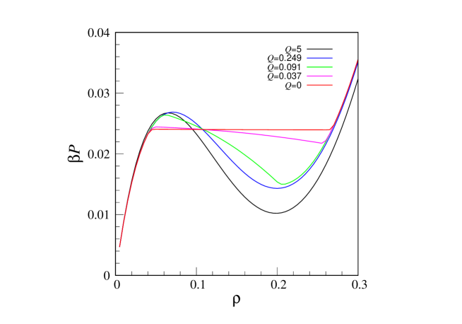
Figure 8: The HRT equation of state (reduced pressure vs. density) of the model defined in Eq. (4.2) for $\eta=0.025$ at different values of the cut-off $Q$. The initial condition at $Q=5$ is given by the mean-field approximation (black line). Integration of the “evolution equation” (3.1) allows to gradually include density fluctuations. The equation of state is shown for a few representative intermediate values of the cut-off: $Q=0.249$ (blue), $Q=0.091$ (green), and $Q=0.037$ (magenta), till $Q=0$ (red), where convexity of free energy is eventually recovered.

An illustrative example, displaying the role of fluctuations in suppressing van der Waals loops, is shown in Fig. 8 of Sec. IV.B. The equation of state of the shifted double-Gaussian model (defined at Eq. (4.2) below) for $\eta=0.025$ is plotted for different values of the cut-off $Q$, at a reduced temperature $T=0.12<T_{c}$. When $Q$ is large, the free energy is given by its mean-field value, and a van der Waals loop is clearly present. As $Q$ is decreased, density fluctuations of wave-vector $Q$ are gradually included, leading, for $Q=0$, to the complete suppression of the loop: A region of constant pressure now appears in the density interval $0.05<\rho<0.265$, allowing the unambiguous identification of the coexistence region at $T=0.12$.

III.3 Monte Carlo simulation

In Ref. Malescio_Prestipino , we have investigated liquid-vapor coexistence in a shifted-DG system near the stability threshold, using the method of Gibbs-ensemble Monte Carlo (GEMC) simulation Panagiotopoulos ; Frenkel . Here, the same analysis is performed for a DE type of system (see Sec. IV.B).

In a GEMC simulation run, $N$ particles are initially distributed between two cubic simulation boxes, and arranged in, e.g., a lattice configuration with the same number density in both. Periodic boundary conditions are applied to each box separately. One GEMC cycle consists of trial moves of three types: shift of a particle within a box, exchange of volume between the boxes, and particle swap. The acceptance rule as well as the schedule of the moves are designed in such a way that detailed balance holds; particular care has been paid in treating the case where one box happens to be empty (see Ref. Frenkel , which we have closely followed in writing our GEMC code). In order to achieve faster equilibration at low temperature we have found useful to start with largely different numbers of particles in the two boxes (in the captions of Figs. 8 and 9 below, we write $N_{1}+N_{2}$ to mean that we initially put $N_{1}$ particles in one box and $N_{2}$ particles in the other). Typically, from $4\times 10^{4}$ to $4\times 10^{5}$ GEMC cycles (depending on the sample size) are more than enough for equilibrium quantities like the density or the energy, whose averages are computed over the second half of the trajectory only.

IV Results

IV.1 HNC results

For each potential of those listed in Sec. II, we have examined first how the BL changes upon varying the balance between repulsive and attractive interactions. We focus on an interval of values of the potential parameters lying close to the TST.

Though the HNC equation can only provide a qualitative assessment of the fluid phase diagram, it turns out that it is extremely accurate in locating the ultimate threshold of thermodynamic stability. As shown below, for all the investigated systems we find that the HNC estimate of the TST is in excellent agreement with the analytic result derived from the Ruelle-Fisher criteria (relative differences being of the order of $10^{-3}$, or even smaller). Therefore, we can confidently assume that, at least in a small interval around the threshold, the HNC equation is able to grasp the essential features of the fluid behavior. At the end of the section, we present a theoretical argument to justify the effectiveness of the HNC equation for FRAC fluids.

1) DG potential. For fixed $A,B,b$, the DG potential (2.1) only depends on the $a$ parameter. As $a$ increases, the repulsion becomes more and more short-ranged, hence the interval of distances over which the attractive component is effective grows, and the depth of the attractive well also increases. Clearly, the attraction can be enhanced relative to repulsion in many different ways; for example, at fixed $A,a,b$, an increase of $B$ makes the attractive well deeper, while the attractive range is not affected. Otherwise, one can extend the range of the attractive well (controlled by $b$) while keeping its depth ($B$) fixed. In general, for any given potential one can use different parameters to control the importance of attraction versus repulsion. The choice of the control parameter determines the way in which attraction grows at the expense of repulsion as the system approaches thermodynamic instability. Alternatively, one may consider many different potential forms and study their behavior in the approach to thermodynamic instability as only one of the possible control parameters is varied. In our analysis we followed the latter option, which allows a more thorough investigation of the space of interaction potentials.

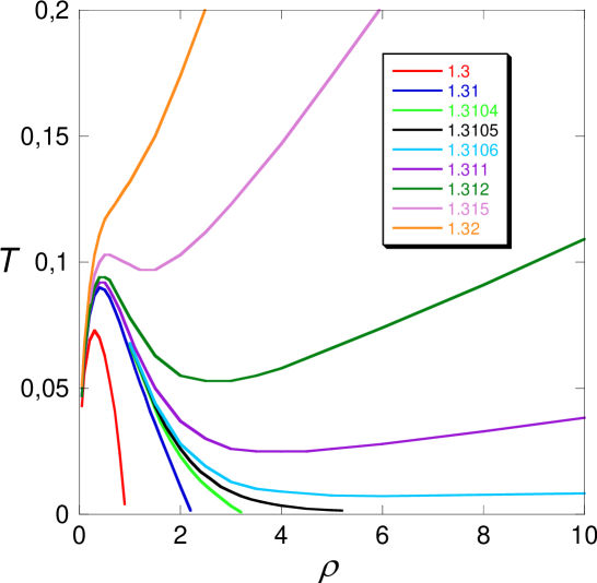
Figure 1: DG potential for $A=1.5,B=b=1$: BL for a few values of $a$ (in the legend), growing from bottom to top. In this picture, as well as in the following ones, both $\rho$ and $T$ are expressed in dimensionless units.

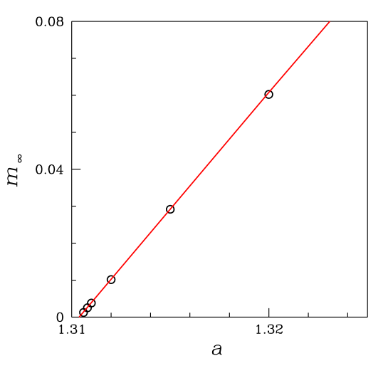
Figure 2: DG potential for $A=1.5,B=b=1$: asymptotic BL slope $m_{\infty}$ for a number of $a$ values (open dots). A linear least-square fit of the data points gives $a^{\prime}_{c}=1.31040247$, to be compared with $a_{c}=1.31037069\ldots$ The red line represents $|\widetilde{u}(0)|$ as a function of $a$ (see Sec. IV.C). The $r$ grid used in the computer code to solve the HNC equation has 2048 points and a spacing of 0.01 (see text).

In Fig. 1 we plot the BL for $A=1.5$ and $B=b=1$ in a range of $a$ values enclosing the TST ($a=a_{c}=1.31037069\ldots$). We see in this picture that, for small $a$, the unstable-fluid region is bell-shaped and its area is finite; above the temperature $T_{\rm max}$, corresponding to the bell maximum, the HNC equation can be solved for any $\rho$. As $a$ increases, the unstable-fluid region becomes higher ($T_{\rm max}$ increases) and wider. In the proximity of $a_{c}$, the widening of the curve blows up at low $T$, until the liquid density apparently diverges for $T\rightarrow 0$ at $a=a^{\prime}_{c}\simeq a_{c}$. In analogy to the evolution of the liquid-vapor binodal line in the shifted-DG model Malescio_Prestipino , we surmise that $a^{\prime}_{c}$ is the HNC estimate of $a_{c}$. For $a>a^{\prime}_{c}$ the topology of the BL changes radically: the right side of the bell “opens up” and, at large densities, the BL becomes a straight line with positive slope. In other words, for all $T$ there is a density above which the HNC equation cannot be solved. Accordingly, the area of the unstable-fluid region becomes infinite. As $a$ increases further, the BL becomes monotonically increasing, and eventually resembles a straight line running close to the $T$ axis; in turn, the unstable-fluid region covers the entire thermodynamic plane, except only for a narrow region of low densities.

In order to estimate $a^{\prime}_{c}$ accurately, we proceed as follows. At $a=a^{\prime}_{c}$, the BL has a vanishing asymptotic slope. We calculate for $a>a^{\prime}_{c}$ the slope $m_{\infty}$ of the BL at very high density (where the BL is a perfectly straight line) and report it in a graph as a function of $a$ (Fig. 2). We find that these slopes lie on a straight line, meaning that the BL slope is to a very good approximation a linear function of $a$, at least close enough to $a^{\prime}_{c}$. Through a least-square fit, we extrapolate $m_{\infty}(a)$ down to zero slope, thus obtaining the crossover value $a^{\prime}_{c}$ between the stable and the Ruelle-unstable regime. We stress that $m_{\infty}(a)$ is close to a straight line for all the $a>a^{\prime}_{c}$ values considered in Fig. 1, regardless of the shape of the BL at low density.

Obviously, the accuracy of $a^{\prime}_{c}$ depends on the $r$ grid used to solve the HNC equation by iteration. Throughout this paper, we use a spatial grid with $N=2^{10}$ points and spacing $0.02$ (we have performed a few checks with more refined grids and found no appreciable variation in the overall BL behavior). We obtain $a^{\prime}_{c}=1.3105168$, which is extremely close to $a_{c}$ (the difference is 0.00015). Using a denser mesh of points ($N=2^{11}$, with spacing $0.01$) we obtain the even more accurate estimate $a^{\prime}_{c}=1.31040247$ (corresponding to a difference $a^{\prime}_{c}-a_{c}$ of 0.000032). A similar systematic improvement in accuracy is found for all the potentials considered.

Table 1: DG potential for $B=b=1$: For a few $A$ values we compare the TST $a_{c}$ with its estimate $a^{\prime}_{c}$ from the HNC theory. The $a^{\prime}_{c}$ data have been computed with a $r$ grid of 1024 points and a spacing of 0.02 (see text).

$A$	$a_{c}$	$a^{\prime}_{c}$
1.5	1.3104	1.31052(1)
2	1.5874	1.5875(5)
3	2.0801	2.0805(5)

In Table I we report $a^{\prime}_{c}$ for a few values of $A$, and compare it to the TST (according to the Ruelle-Fisher criteria, $A/B\geq(a/b)^{3/2}\geq 1$ is a necessary and sufficient condition for thermodynamic stability Heyes1 ). It turns out that $a^{\prime}_{c}$ is in remarkable agreement with the threshold $a_{c}$, the relative discrepancy being smaller than $0.001$.

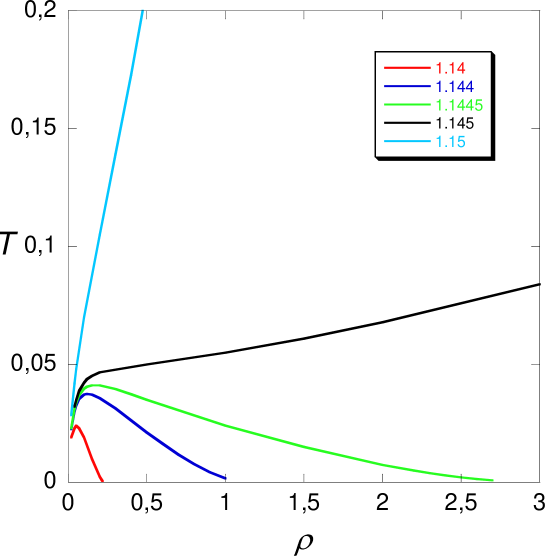
Figure 3: DE potential for $A=1.5,B=b=1$: BL for a few values of $a$ (in the legend), growing from bottom to top.

Table 2: DE potential for $B=b=1$: For a few $A$ values we compare the TST $a_{c}$ with its estimate $a^{\prime}_{c}$ from the HNC theory.

$A$	$a_{c}$	$a^{\prime}_{c}$
1.5	1.1447	1.1447(3)
2	1.2599	1.2595(5)
3	1.4422	1.4425(5)

2) DE potential. For fixed $A,B,b$, the DE potential (2.2) only depends on $a$. As $a$ increases, the repulsion becomes more short-ranged and the importance of the attraction in turn increases. The evolution of the BL with increasing $a$ (see Fig. 3) is similar to that reported for the DG potential.

In Table II we report $a^{\prime}_{c}$ for a few values of $A$, while $a_{c}$ follows from the Ruelle-Fisher criteria, according to which $A/B>(a/b)^{3}$ is a necessary and sufficient condition for thermodynamic stability Heyes1 . The relative discrepancy between the HNC threshold and the exact one is smaller than 0.001.

3) CG potential. According to the Ruelle-Fisher criteria, $a^{2}/(2b)\leq 1$ is a necessary and sufficient condition for thermodynamic stability Heyes1 . A CG-type of potential has been considered by Louis et al. Louis2 , who write it in the form:

$$u(r)=\cos\left(\sqrt{2+\delta}\,r\right)\exp\{-r^{2}\}$$ (4.1)

(i.e., $a=\sqrt{2+\delta},b=1$). Hence, the stability criterion for (4.1) reads $\delta\leq 0$. Our analysis based on the HNC equation yields a threshold value $\delta^{\prime}_{c}=0.001(1)$ (see Fig. 4).

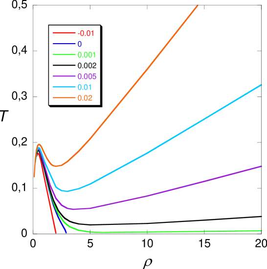
Figure 4: CG potential (4.1): BL for a few values of $\delta$ (in the legend), growing from bottom to top.

4) SHRAT potential. According to the Ruelle-Fisher criteria, $A/B\geq 7/4$ is a necessary and sufficient condition for thermodynamic stability Heyes1 . For $B=1$, the HNC analysis gives $A^{\prime}_{c}=1.7497(5)$ (see Fig. 5). Notice that the path from the stable to the Ruelle-unstable regime corresponds for the SHRAT potential to the direction of decreasing $A$.

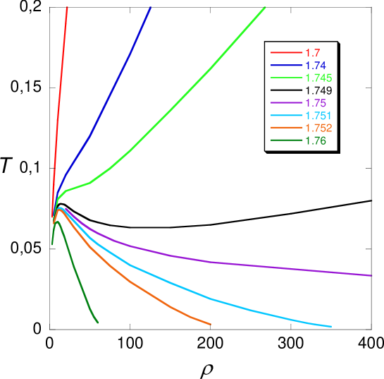
Figure 5: SHRAT potential for $B=1$: BL for a few values of $A$ (in the legend), growing from top to bottom.

5) Separation-shifted LJ potential. In Ref. Heyes2 , the conditions for stability of potential (2.5) have been investigated for $p=6$ and $q=3$ (which yields a regularized LJ potential), and it has been found for $a=b$ that $A/B\geq 32/7=4.5714\ldots$ is a necessary and sufficient condition for thermodynamic stability. For $B=1$, the HNC equation predicts a threshold value $A^{\prime}_{c}=4.569(1)$ (see Fig. 6). Again, the system turns from stable to Ruelle-unstable upon decreasing the value of $A$.

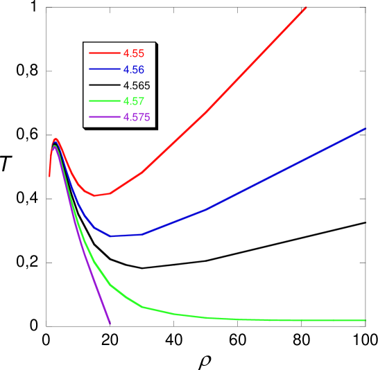
Figure 6: Separation-shifted LJ potential ($a=b,B=1,p=6,q=3$): BL for a few values of $A$ (in the legend), growing from top to bottom.

6) GE6 potential. The Fourier transform of the GE6 potential in Eq. (2.6) is negative at the origin for $Ab^{6}/B<\pi(ab)^{3}/32$ Heyes1 . However, $\widetilde{u}(k)$ is not positive definite for $Ab^{6}/B\geq\pi(ab)^{3}/32$, hence one cannot state — based only on the Ruelle-Fisher criteria — that the system is thermodynamically stable above this threshold. However, the HNC analysis indicates that this is likely the case. We have computed the BL for $B=b=1,a=3$, and several $A$ values (see Fig. 7; notice that the system turns from stable to Ruelle-unstable with decreasing $A$). By fitting the asymptotic BL slopes for $A=2.6,2.62,2.64$, we obtain $A^{\prime}_{c}=2.6503(2)$, close indeed to the TST value ($A_{c}=2.6507$). We have checked numerically that, for $A=2.65$, the BL indeed attains a minimum for a density $\rho\approx 200$.

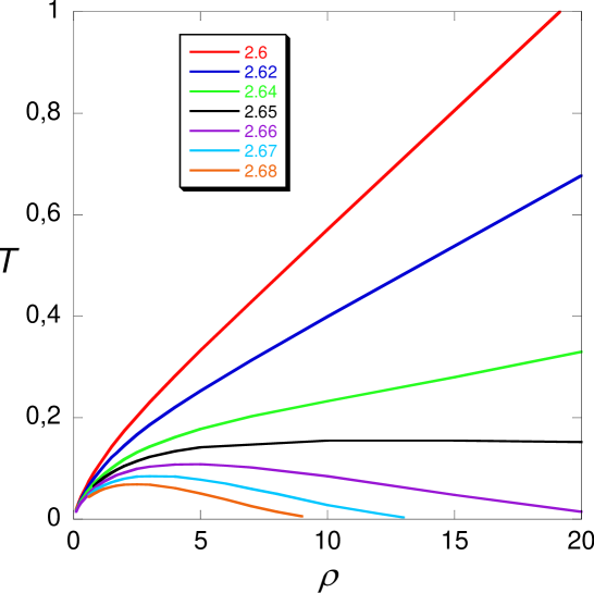
Figure 7: GE6 potential for $B=b=1,a=3$: BL for a few values of $A$ (in the legend), growing from top to bottom.

IV.2 Comparison with HRT and MC results

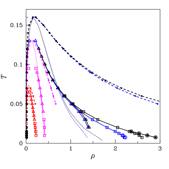
Figure 9: Shifted-DG potential (see Eq. (1) of Ref. Malescio_Prestipino ) below $\eta_{\rm c}=0.02631579\ldots$: Liquid-vapor coexistence densities from GEMC simulations performed for a number of $\eta$ values (0.020, red; 0.025, magenta; 0.0263, blue; and 0.02631, black). The various symbols correspond to different initial numbers of particles in the two simulation boxes ($864+864$, triangles; $4000+108$, squares; $8192+128$, open dots; and $16000+128$, full dots). Also reported are the BL and the HRT coexistence densities for the same $\eta$ values (dotted and dashed lines, respectively).

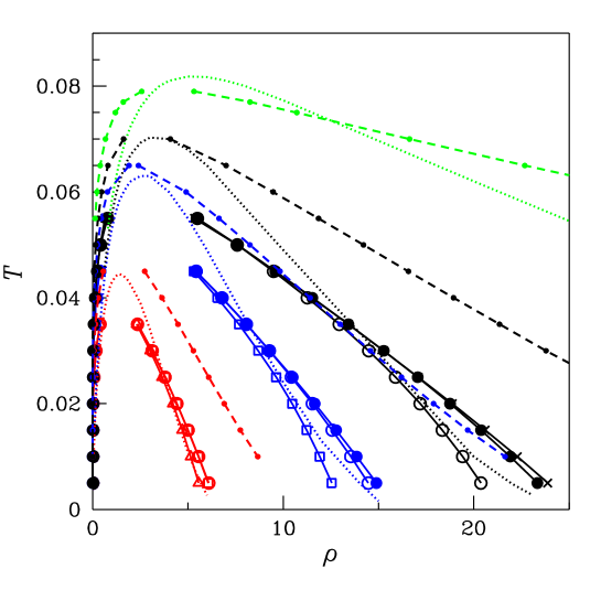
Figure 10: DE potential (4.2) above $L_{c}=0.79370052\ldots$: Liquid-vapor coexistence densities from GEMC simulations performed for a number of $L$ values (0.80, red; 0.796, blue; and 0.795, black). The various symbols correspond to different initial numbers of particles in the two simulation boxes ($864+864$, triangles; $4000+256$, squares; $8192+250$, open dots; $16000+128$, full dots; and $32000+256$, crosses). Also reported are the BL and HRT coexistence densities as dotted and dashed lines, respectively (the green lines are for $L=0.794$).

For the same shifted-DG potential investigated in Ref. Malescio_Prestipino , i.e.,

$$u(r)=\exp\{-r^{2}\}-\eta\exp\{-(r-3)^{2}\}\,,$$ (4.2)

we have used the HRT to compute a number of points along the binodal line for a few values of $\eta$ (the attraction strength). Adding these points to the MC data points in Fig. 1 of Ref. Malescio_Prestipino , we finally obtain the present Fig. 9. As $\eta$ moves towards $\eta_{c}$, the HRT binodal line shows the characteristic widening already observed in the BL and in the MC data. Moreover, the HRT binodal line satisfactorily encloses the HNC pseudospinodal line. In more quantitative terms, however, the HRT substantially overestimates the densities of the coexisting liquid.

As a second example, we have considered the following one-parameter family of DE potentials,

$$u(r)=2\exp\{-3r/L\}-\exp\{-3r\}\,.$$ (4.3)

The TST of potential (4.3) is $L_{c}=2^{-1/3}$ (see Sec. IV.A). In order to speed up the simulation, the potential has been cut off at $r=5$. We have carried out GEMC simulations on samples of increasing size, until finite-size effects vanish altogether. We have checked that, once formed, the liquid always occupies the box of larger volume (otherwise, the simulation is restarted from a different configuration). The BL, the MC coexistence line for various sizes, and the HRT binodal line are all reported in Fig. 10. Overall, the same scenario of Fig. 9 shows up, with the HRT line considerably wider than the MC line, especially closer to $L_{c}$. Despite this, the behavior of the HRT line qualitatively reproduces the MC coexistence line.

As a last comment, we point out that we have never observed in our simulations the spontaneous onset of a crystalline phase. This means that, either a stable crystal only occurs at densities considerably higher than those probed here, or the liquid phase is actually metastable but its lifetime is very long. In any event, the possible metastability of the liquid phase at the highest densities would not weaken in any respect the expectation, corroborated by simulation in two distinct cases, of an anomalous widening of the liquid-vapor coexistence line of FRAC fluids approaching the TST from below.

IV.3 Theory

In order to account for the BL behavior described in Sec. IV.A, and thus unveil the roots of universality in the approach of FRAC fluids to the TST, we put forward an argument that builds on that presented in Ref. Malescio_Prestipino but considerably extend it. In the following, the ultimate threshold of stability of the homogeneous fluid is identified with the locus $T_{0}(\rho)$ where the inverse isothermal compressibility, given in general by

$$\frac{1}{\rho k_{B}TK_{T}}=\frac{1}{1+\rho\widetilde{h}(0)}=1-\rho\widetilde{c}(0)\,,$$ (4.4)

is predicted to vanish.

In Ref. Malescio_Prestipino , we have made the hypothesis that, for each FRAC fluid, a characteristic density $\rho_{0}(T)$ exists above which the total correlation function

$$h(r)\approx 0\,,$$ (4.5)

that is, $h$ is zero for all distances to within a small tolerance fixed once and for all (we have checked that Eq. (4.5) is roughly satisfied in MC simulations of the shifted-DG fluid along the $\rho=5$ isochore). We expect that $\rho_{0}(T)$ is a decreasing function of $T$, because the higher is the temperature the better the system would conform to ideal-gas behavior. Equation (4.5) tells that the structure of a FRAC fluid at high enough density resembles that of an ideal gas (“infinite-density ideal gas” limit Stillinger ; Likos1 ).

This ansatz is actually a direct consequence of the form of the HNC equation:

$$c(r)=h(r)-\ln[1+h(r)]-\beta u(r)$$ (4.6)

In fact, by spatial integration of both sides of Eq. (4.6), we get $\widetilde{c}(0)=\int{\rm d}{\bf r}\,\left\{h(r)-\ln[h(r)+1]\right\}-\beta\widetilde{u}(0)$. The HNC equation, by encompassing the Ornstein-Zernike equation, has solutions only provided that $\widetilde{c}(0)<1/\rho$, which implies $\int{\rm d}{\bf r}\,\left\{h(r)-\ln[h(r)+1]\right\}<\beta\widetilde{u}(0)+1/\rho$. Close to the Fisher-Ruelle stability threshold and at high density, the right-hand side is small and thermodynamic stability then implies that also the left-hand side is small. However, the integrand is positive semidefinite and vanishes only for $h(r)=0$. As a consequence, in this limit the HNC equation forces the total correlation function to small values at all distances.

If Eq. (4.5) holds, for $\rho>\rho_{0}(T)$ we obtain from the HNC equation that

$$c(r)=h(r)-\ln[1+h(r)]-\beta u(r)\approx-\beta u(r)\,,$$ (4.7)

namely, at sufficiently high density the HNC approximation reduces to the random phase approximation (RPA). Taken the RPA for granted, we have:

$$\frac{1}{\rho k_{B}TK_{T}}=1+\beta\widetilde{u}(0)\rho\,.$$ (4.8)

Hence, $K_{T}$ is always positive in the stable regime, where $\widetilde{u}(0)>0$, while it is negative beyond the density $k_{B}T/|\widetilde{u}(0)|$ in the unstable regime (for the sake of clarity, we hereafter use a notation appropriate to the shifted-DG potential Malescio_Prestipino ; Prestipino_Malescio , where the stable regime corresponds to $\eta<\eta_{c}$; however, similar considerations apply for each parametric FRAC potential which becomes Ruelle-unstable exactly where $\widetilde{u}(0)$ changes sign). While the previous conclusions are consistent with the high-density behavior of the BL for $\eta>\eta_{c}$ Malescio_Prestipino , they are clearly insufficient to explain its anomalous widening below $\eta_{c}$.

Reasoning in purely heuristic terms, a better approximation for large densities would be:

$$\widetilde{c}(0)=-\beta\widetilde{u}(0)+\frac{A}{\rho}\,,$$ (4.9)

$A$ being a dimensionless quantity. From Eq. (4.4), it then follows:

$$\frac{1}{\rho k_{B}TK_{T}}=1+\beta\widetilde{u}(0)\rho-A\,.$$ (4.10)

Aiming to reproduce the HNC phenomenology at high density, we assume that $A=T^{*}/T$, for a convenient $T^{*}$. This is a reasonable assumption, considering that Eq. (4.6) becomes better satisfied, at fixed density, when $T$ is higher. With this $A$, we obtain:

$$K_{T}>0\,\,\,\Longleftrightarrow\,\,\,k_{B}T>k_{B}T^{*}-\widetilde{u}(0)\rho\,.$$ (4.11)

Below $\eta_{c}$, Eq. (4.11) predicts that the BL is a straight line for high densities. Stated differently, Eq. (4.11) reads:

$$K_{T}>0\,\,\,\Longleftrightarrow\,\,\,\rho>\frac{k_{B}(T^{*}-T)}{\widetilde{u}(0)}\,.$$ (4.12)

In particular, at $T=0$ the system would be stable only for densities larger than

$$\rho^{*}=\frac{k_{B}T^{*}}{\widetilde{u}(0)}\,,$$ (4.13)

which grows and eventually diverges when $\eta$ goes to $\eta_{c}$. Very close to $\eta_{c}$, where $\widetilde{u}(0)\approx B(\eta_{c}-\eta)$ with $B>0$, an immediate prediction is $\rho^{*}\propto(\eta_{c}-\eta)^{-1}$. However, we find that this scaling law is not generally obeyed, which can only be the effect of a $\rho_{0}(T)$ diverging for $T\rightarrow 0$ faster than $\rho^{*}$. Indeed, we have checked in a few cases that the radial structure of the saturated liquid near $T=0$ is anything but trivial in the HNC theory. We conclude that, even though the simple modification (4.9) to the RPA correctly accounts for the general blowing up of $\rho^{*}$ at $\eta_{c}$, it is by far insufficient to give the correct scaling exponent (which, moreover, appears to be non-universal).

Above $\eta_{c}$, where the HNC equation can still be solved, we obtain from Eq. (4.11):

$$K_{T}>0\,\,\,\Longleftrightarrow\,\,\,k_{B}T>k_{B}T^{*}+|\widetilde{u}(0)|\rho\,.$$ (4.14)

In particular, the asymptotic slope of the BL above $\eta_{c}$ is just $|\widetilde{u}(0)|$, as already checked to a very high precision in the shifted-DG potential Malescio_Prestipino (see also Fig. 2). Stated differently, the stability condition reads

$$\rho<\frac{k_{B}(T-T^{*})}{|\widetilde{u}(0)|}\,,$$ (4.15)

and is clearly violated for $T=0$, with the result that the unstable-fluid region now extends to infinite density.

V Conclusions

We have shown that a considerable number of FRAC potentials exhibit similar fluid behavior when the threshold of thermodynamic (alias H-) stability is approached, and eventually surpassed. The most important feature of this general behavior is the pronounced widening of the binodal line at low $T$. Right at the TST, a vanishing-density vapor coexists with a diverging-density liquid. This is consistent with the long-time behavior of the shifted double-Gaussian fluid beyond the TST Malescio_Prestipino ; Prestipino_Malescio , where $N$ particles collapse to an extremely dense aggregate and the energy per particle is proportional to $N$. Given the widely different features of the systems examined in this paper, our results suggest that the transition of FRAC fluids to Ruelle instability indeed occurs following a universal pathway.

Using the HNC pseudospinodal line as a clue to liquid-vapor coexistence behavior, we have found that the HNC estimate of the TST is, for all the investigated systems, in excellent agreement with the value provided by the Ruelle-Fisher criteria. This supports the assumption that, at least in a narrow interval around this threshold, the HNC equation gives reliable indications. For two specific interactions (the shifted-DG and DE potentials), the predictions of the HNC equation have been checked against MC simulation and a more refined liquid-state theory, the HRT. By this comparison, we conclude that the HNC equation faithfully describes the modifications undergone by the liquid-vapor coexistence line as the TST is approached from the stable side. We argue that this happens as a result of the nearly ideal-gas structure of the high-density fluid, as illustrated in Sec. IV.C, where we have put forward a general explanation for the universal approach of a bounded potential to the TST, by an argument that supersedes and improves the original one given in Ref. Malescio_Prestipino .

In the light of the present results, it is possible to build up the following general scenario for the transition to Ruelle instability in fluid systems with a bounded interparticle repulsion and a longer-range attraction. For stable homogeneous fluids, there exists a region of mechanical instability (bounded above by the spinodal line) lying inside that of thermodynamic instability (bounded above by the binodal line). Both regions occupy a bounded subset of the thermodynamic plane. Upon getting closer to the threshold of Ruelle instability, the extension of both regions increases due to widening of both binodal and spinodal lines at low temperatures. When the TST is eventually reached, the liquid density becomes infinitely large for $T\rightarrow 0$. In the HNC analysis, the transition to the Ruelle-unstable regime is evidenced in the “opening up” of both thermodynamic and mechanical unstable-fluid regions, i.e., the extension of these regions on the $\rho$-$T$ plane turns from bounded to unbounded at the crossing of the TST.

References

- (1) A. A. Louis, P. G. Bolhuis, J.-P. Hansen, and E. J. Meijer, Phys. Rev. Lett. 85, 2522 (2000).
- (2) C. N. Likos, Phys. Rep. 348, 267 (2001).
- (3) C. N. Likos, M. Schmidt, H. Löwen, M. Ballauff, D. Pötschke, and P. Lindner, Macromolecules 34, 2914 (2001).
- (4) C. N. Likos, Soft Matter 2, 478 (2006).
- (5) D. Ruelle, Statistical Mechanics: Rigorous Results (Imperial College Press, London, 1999).
- (6) M. E. Fisher and D. Ruelle, J. Math. Phys. 7, 260 (1966).
- (7) D. M. Heyes and G. Rickayzen, J. Phys.: Condens. Matter 19, 416101 (2007).
- (8) S. Prestipino, C. Speranza, G. Malescio, and P. V. Giaquinta, J. Chem. Phys. 140, 084906 (2014).
- (9) C. Speranza, S. Prestipino, G. Malescio, and P. V. Giaquinta, Phys. Rev. E 90, 012305 (2014).
- (10) G. Malescio and S. Prestipino, Phys. Rev. E 92, 050301(R) (2015).
- (11) S. Prestipino and G. Malescio, Physica A 457, 492 (2016).
- (12) R. Fantoni, A. Malijevský, A. Santos, and A. Giacometti, Europhys. Lett. 93, 26002 (2011).
- (13) R. Fantoni, A. Malijevský, A. Santos, and A. Giacometti, Mol. Phys. 109, 2723 (2011).
- (14) M. R. D’Orsogna, Y. L. Chuang, A. L. Bertozzi, and L. S. Chayes, Phys. Rev. Lett. 96, 104302 (2006).
- (15) M. A. Miller, J. P. K. Doye, and D. J. Wales, J. Phys. Chem. 110, 328 (1999).
- (16) I. Stankovic, S. Hess, and M. Kröger, Phys. Rev. E 69, 021509 (2004).
- (17) D. M. Heyes, M. J. Cass, and G. Rickayzen, J. Chem. Phys. 126, 084510 (2007).
- (18) R. A. Buckingham and J. Corner, Proc. Royal Soc. A 189, 118 (1947).
- (19) F. Saija and S. Prestipino, Phys. Rev. B 72, 024113 (2005).
- (20) G. Malescio, F. Saija, and S. Prestipino, J. Chem. Phys. 129, 241101 (2008).
- (21) See, e.g., J.-P. Hansen and I. R. McDonald, Theory of Simple Liquids, 4th ed. (Academic, New York, 2013).
- (22) C. N. Likos, B. M. Mladek, D. Gottwald, and G. Kahl, J. Chem. Phys. 126, 224502 (2007).
- (23) A. Parola and L. Reatto, Mol. Phys. 110, 2859 (2012).
- (24) P. G. Bolhuis, A. A. Louis, J.-P. Hansen, and E. J. Meijer, J. Chem. Phys. 114, 4296 (2001).
- (25) A. Z. Panagiotopoulos, Mol. Phys. 61, 813 (1987).
- (26) See, e.g., D. Frenkel and B. Smit, Understanding Molecular Simulation, 2nd ed. (Academic, 2002).
- (27) A. A. Louis, P. G. Bolhuis, and J.-P. Hansen, Phys. Rev. E 62, 7961 (2000).
- (28) F. H. Stillinger, J. Chem. Phys. 65, 3968 (1976).