Electric and Magnetic Gating of Rashba-Active Weak Links

Abstract

In a one-dimensional weak-link wire the spin-orbit interaction (SOI) alone cannot generate a nonzero spin current. We show that a Zeeman field acting in the wire in conjunction with the Rashba SOI there does yield such a current, whose magnitude and direction depend on the direction of the field. When this field is not parallel to the effective field due to the SOI, both the charge and the spin currents oscillate with the length of the wire. Measuring the oscillating anisotropic magnetoresistance can thus yield information on the SOI strength. These features are tuned by applying a magnetic and/or an electric field, with possible applications to spintronics.

Spintronics takes advantage of the electronic spins in designing a variety of applications, including giant magnetoresistance sensing, quantum computing, and quantum-information processing wolf ; zutic . A promising approach for the latter exploits mobile qubits, which carry the quantum information via the spin polarization of the moving electrons. The spins of mobile electrons can be manipulated by the spin-orbit interaction (SOI), which causes the spin of an electron moving through a spin-orbit active material (e.g., semiconductor heterostructures Kohda ) to rotate around an effective magnetic field that depends on the momentum winkler ; manchon . In the particular case of the Rashba SOI rashba , both the rotation axis and the amount of rotation can be tuned by gate voltages Nitta ; Sato ; Beukman ; comDres . Research in this direction was enhanced following the proposal by Datta and Das datta , of a spin field-effect transistor based on magnetic leads. It is still a challenge to achieve polarized mobile electronic spins avoiding the use of ferromagnetic leads.

In the simplest device, electrons move between two large electronic reservoirs, via a mesoscopic region. When the region is spin-orbit active, the single-channel transmission is described by a $2\times 2$ matrix in spin Hilbert space. Since this matrix is proportional to the unit matrix when time-reversal symmetry is obeyed bardarson , spin splitting cannot be achieved with SOI alone. Time-reversal symmetry is broken by applying a magnetic field. Indeed, several proposed devices utilize an orbital Aharonov-Bohm magnetic flux, which penetrates loops of interferometers to achieve spin splitting lyanda ; us ; Saarikoski , via the interference of the spinor wave functions in the two branches of the loop.

Here we analyze an even simpler geometry: the two reservoirs are connected by a single (weak link) spin-orbit active wire, but we do take into account the Zeeman energy gained from an external magnetic field acting on the whole wire (see Fig. 1). Due to this field, both the charge and the spin conductances of the device are found to exhibit oscillations with the length of the wire. These oscillations, as well as the associated magnetoconductance anisotropy, can be used to identify the strength of the SOI; remarkably, they can be tuned by applying electric and/or magnetic fields. Although earlier papers privman ; goldhaber ; gudmundsson considered the band structure and the gate-voltage dependence of the conductance of such wires, they did not discuss these interesting phenomena.

The SOI and the Zeeman field split the spinor wave function in the wire into two waves, with different wave vectors and with different spin polarizations. In the presence of both the external magnetic field, ${\bf H}$, and the effective magnetic field due to the SOI, ${\bf H}_{\rm so}$, each of these accumulates its own phase along the link, and they interfere to generate a 2$\times$2 matrix for the tunneling amplitude, which contains a mixture of the two polarizations. Without the external field, this matrix is unitary, causing only a rotation of the spin polarizations around ${\bf H}_{\rm so}$ by an angle which depends on the SOI strength and the wire length Oreg . The resulting transmission matrix is proportional to the unit matrix, and there is no net polarization. In contrast, a nonzero ${\bf H}$ generates a non-unitary tunneling amplitude. Then, a bias voltage between the reservoirs induces particle and spin currents. Thus, the non-unitarity of the transmission matrix results in a net spin magnetization in the reservoirs. This, as well as the magnetoconductance of the weak link, do not depend on the length of the wire unless the magnetic field is not along ${\bf H}_{\rm so}$. In particular, when ${\bf H}$ is perpendicular to ${\bf H}_{\rm so}$, both properties exhibit distinct oscillations with this length, on length scales related to the SOI and the field strengths. As such, they are both tunable by electric and magnetic fields. The magnetization generated in the reservoirs has components along ${\bf H}$ and ${\bf H}_{\rm so}$, and - surprisingly - also perpendicular to both of these directions. Remarkably, these effects are of the order of the ratio of the Zeeman energy to the spin-orbit energy comAB .

The described interference can be compared to the Aharonov-Bohm effect, where the electron wave function acquires different extra phases from the motion of an electric charge along different paths in an external magnetic field. Here the extra phases - which we may call Aharonov-Casher AC phases for electrons - are due to the motion of a magnetic moment in an electric field. Our device can therefore be viewed as an Aharonov-Casher interferometer. Unlike the Aharonov-Bohm one, here the phase difference between two “channels” can appear even though the electrons move along the same spatial trajectory between two singly-connected leads.

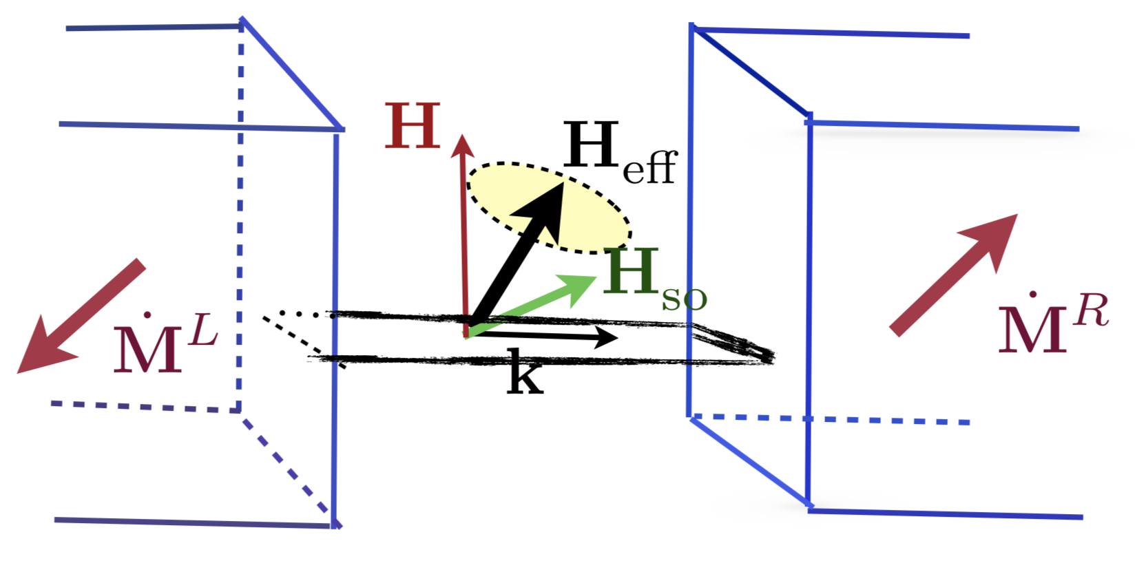
Figure 1: (Color online.) A spin-orbit active weak-link wire connecting two reservoirs. The momentum of the electron is ${\bf k}$, the external magnetic field is ${\bf H}$ and the effective field due to the SOI is ${\bf H}_{\rm so}$. The net effective field (around which the spins rotate) is ${\bf H}_{\rm eff}$. The arrows in the reservoirs show the magnetization rates there, $\dot{\bf M}^{L}$ and $\dot{\bf M}^{R}=-\dot{\bf M}^{L}$, generated due to the joint effect of ${\bf H}_{\rm so}$ and ${\bf H}$.

Adopting units in which $\hbar=1$ and using the linear Rashba SOI, the Hamiltonian of the system is

$${\cal H}={\cal H}_{\rm link}+{\cal H}_{\rm leads}+{\cal H}_{\rm tun}\ .$$ (1)

Here, the Hamiltonian in the weak link is

$${\cal H}_{\rm link}=-\frac{1}{2m^{\ast}}{\mbox{\boldmath{$\nabla$}}}^{2}-i\frac{\widetilde{k}_{\rm so}}{m^{\ast}}\hat{\bf n}\cdot({\mbox{\boldmath{$\sigma$}}}\times{\mbox{\boldmath{$\nabla$}}})-{\bf H}\cdot{\mbox{\boldmath{$\sigma$}}}\ ,$$ (2)

where $\sigma$ is the vector of Pauli matrices, $m^{\ast}$ is the effective mass, and $\hat{\bf n}$ is a unit vector along the electric field which causes the SOI. The net strength of this interaction (in momentum units comRashba ) is denoted $\widetilde{k}_{\rm so}$; the notation $k_{\rm so}$ is used below for the “full” coupling. The “magnetic field” ${\bf H}$ contains the factor $(g/2)\mu_{\rm B}$, i.e., the $g-$factor and the Bohr magneton, and therefore has units of energy. The Hamiltonian of the leads is ${\cal H}_{\rm leads}=\sum_{\alpha=L,R}{\cal H}^{\alpha}_{\rm lead}$, with

$${\cal H}^{\alpha=L(R)}_{\rm lead}=\sum_{{\bf k}({\bf p}),\sigma}\epsilon_{k(p)}c^{\dagger}_{{\bf k}({\bf p})\sigma}c_{{\bf k}({\bf p})\sigma}\ ,$$ (3)

where $c^{\dagger}_{{\bf k}\sigma}$ ($c_{{\bf k}\sigma}$) creates (annihilates) an electron with momentum ${\bf k}$ and spin $\sigma$ (at an arbitrary quantization axis at this stage) in the left lead, with similar definitions in the right lead. The tunneling between the leads and the weak link is described by

$${\cal H}_{\rm tun}=\sum_{{\bf k},{\bf p},\sigma,\sigma^{\prime}}([V_{{\bf k}{\bf p}}]_{\sigma\sigma^{\prime}}c^{\dagger}_{{\bf k}\sigma}c_{{\bf p}\sigma^{\prime}}+[V^{\ast}_{{\bf k}{\bf p}}]_{\sigma\sigma^{\prime}}c^{\dagger}_{{\bf p}\sigma^{\prime}}c_{{\bf k}\sigma})\ ,$$ (4)

where $[V_{{\bf k}{\bf p}}]_{\sigma\sigma^{\prime}}$ is the tunneling amplitude from the state with momentum ${\bf p}$ and spin $\sigma^{\prime}$ in the right lead to the state with momentum ${\bf k}$ and spin $\sigma$ in the left one. This amplitude, the key ingredient of our approach, is proportional to the spin-dependent propagator connecting the two states revRashba .

Our calculation contains three steps. First, ${\cal H}_{\rm link}$ is used to derive the propagator, i.e., the Green’s function connecting a pair of electronic spin states along the (one-dimensional) wire. Second, the time derivatives of the particle number and the total spin in the reservoirs is found to second-order in ${\cal H}_{\rm tun}$. For unpolarized leads the Fermi distribution, e.g., in the left lead, is

$$f_{L}(\epsilon_{k})=1/[e^{\beta(\epsilon_{k}-\mu_{L})}+1]\ ,$$ (5)

where $\beta=(k_{B}T)^{-1}$ is the inverse temperature and $\mu_{L}$ is the chemical potential. The Fermi distribution in the right reservoir, $f_{R}(\epsilon_{p})$, is defined similarly. Finally, the transmission matrix and the particle and spin currents are analyzed. We consider the case where the Fermi energy in the conducting wire, $E_{\rm F}$ ($E_{\rm F}$ is the common chemical potential of the reservoirs) exceeds significantly all other energies. The opposite limit of an insulating wire ($E_{\rm F}<0$ in our notation) is addressed in Ref. Jonckheere, ; an intriguing interplay between $|E_{\rm F}|$ and both the Zeeman and SOI energies is found to dominate the transport.

We first consider the propagator. Assuming a plane-wave solution with a wave vector ${\bf k}$ directed along the one-dimensional wire, $\exp[i{\bf k}\cdot{\bf r}]=\exp[iks]$ ($s>0$ is the coordinate along the wire), the effective magnetic field associated with the SOI is

$${\bf H}_{\rm so}({\bf k})=(kk_{\rm so}/m^{\ast})\hat{\bf h}_{\rm so}\ ;\quad\hat{{\bf h}}_{\rm so}=(\hat{\bf n}\times\hat{\bf k})/|\hat{\bf n}\times\hat{\bf k}|\ ,$$ (6)

where $k_{\rm so}=\tilde{k}_{\rm so}|\hat{\bf n}\times\hat{\bf k}|$ and $\hat{{\bf h}}_{\rm so}$ is a unit vector along the direction of ${\bf H}_{\rm so}$ comRashba . Then ${\cal H}_{\rm link}({\bf k})=k^{2}/(2m^{\ast})-{\bf H}_{\rm eff}({\bf k})\cdot{\mbox{\boldmath{$\sigma$}}}$, with the net effective magnetic field

$${\bf H}_{\rm eff}({\bf k})={\bf H}_{\rm so}({\bf k})+{\bf H}=\frac{kk_{\rm so}}{m^{\ast}}\hat{\bf h}_{\rm so}+{\bf H}\ .$$ (7)

The (spin-dependent) propagator between two points along the link is a 2$\times$2 matrix in spin space revRashba ; Shahbazyan

$$G(s;E) =\int dke^{iks}\frac{E+i0^{+}-\frac{k^{2}}{2m^{\ast}}-{\bf H}_{\rm eff}({\bf k})\cdot{\mbox{\boldmath{$\sigma$}}}}{(E+i0^{+}-\frac{k^{2}}{2m^{\ast}})^{2}-{H}^{2}_{\rm eff}({\bf k})}\ .$$ (8)

It is evaluated by the Cauchy theorem sup , with $E=k^{2}_{\rm F}/(2m^{\ast})$, as the electrons in the link are at the Fermi energy. The free-particle propagator, $G_{0}(s;E)=-i\pi m^{\ast}\exp[ik_{\rm F}s]/k_{\rm F}$, is recovered when ${\bf H}={\bf H}_{\rm so}=0$.

In the presence of the effective magnetic field Eq. (7), the external magnetic field ${\bf H}$ is decomposed into components parallel ($H_{\parallel}$) and perpendicular ($H_{\perp}$) to $\hat{\bf h}_{\rm so}$. The poles of the integrand in Eq. (8) are the solutions of

$$(k^{2}-k_{\rm F}^{2})^{2}=(2m^{\ast}H_{\perp})^{2}+(2k_{\rm so}k+2m^{\ast}H_{\parallel})^{2}$$ (9)

in the upper half of the complex $k-$plane compole . Denoting these by $k_{\pm}$, with $k^{2}_{\pm}-k_{\rm F}^{2}=\pm 2m^{\ast}H_{\rm eff}(k_{\pm})$, the propagator is

$$G(s;E)=G_{0}(s;E)\exp[-ik_{\rm F}s]$$

$$\times\big{[}e^{ik_{+}s}A_{+}(1+\hat{\bf q}_{+}\cdot{\mbox{\boldmath{$\sigma$}}})+e^{ik_{-}s}A_{-}(1-\hat{\bf q}_{-}\cdot{\mbox{\boldmath{$\sigma$}}})\big{]}\ ,$$ (10)

where the real coefficients $A_{\pm}$ (i.e., the residues of the corresponding poles) and the unit vectors [see Eq. (7)]

$$\hat{\bf q}_{\pm}\equiv \frac{{\bf H}_{\rm eff}(k_{\pm})}{H_{\rm eff}(k_{\pm})}$$ (11)

depend on $k_{\pm}$. The two terms in the square brackets of Eq. (10) correspond to waves with wave numbers $k_{+}$ and $k_{-}$ compole . The corresponding tunneling amplitudes contain the spin projection matrices $(1\pm\hat{\bf q}_{\pm}\cdot{\mbox{\boldmath{$\sigma$}}})$, so that the transmitted electrons are fully polarized along $\hat{\bf q}_{+}$ and $-\hat{\bf q}_{-}$, respectively.

At zero magnetic field $\hat{\bf q}_{+}=\hat{\bf q}_{-}=\hat{\bf h}_{\rm so}$, and the propagator is proportional to a unitary matrix, $G(s;E)\propto\exp[-ik_{\rm so}s\hat{\bf h}_{\rm so}\cdot{\mbox{\boldmath{$\sigma$}}}]$ revRashba . Applied to any spinor, it describes a rotation of its spin polarization, by an amount which is determined by the distance $s$ and by the spin-orbit “momentum” $k_{\rm so}$. This rotation is the same for all spinors, and hence does not change the total spin polarization. As expected from time-reversal symmetry, the SOI alone cannot generate any spin splitting bardarson . In the presence of ${\bf H}$ the matrix in the square brackets in Eq. (10) is not unitary; as shown below, this leads to a finite spin polarization, whose magnitude increases with $H$.

Using these peculiar properties of the spin-dependent tunneling amplitude, we analyze the particle current and the magnetization rate. Both are determined by comsign ; sup

$$R^{L}_{\sigma\sigma^{\prime}}=\frac{d}{dt}\sum_{\bf k}\langle c^{\dagger}_{{\bf k}\sigma}c_{{\bf k}\sigma^{\prime}}\rangle$$

$$=i\sum_{{\bf k},{\bf p},\sigma_{1}}\langle[V^{\ast}_{{\bf k}{\bf p}}]_{\sigma\sigma_{1}}c^{\dagger}_{{\bf p}\sigma_{1}}c_{{\bf k}\sigma^{\prime}}-[V_{{\bf k}{\bf p}}]_{\sigma^{\prime}\sigma_{1}}c^{\dagger}_{{\bf k}\sigma}c_{{\bf p}\sigma_{1}}\rangle\ ,$$ (12)

where the angular brackets indicate a quantum average and where we used the assumption that the leads are not polarized. The total particle current is then

$$I^{L}=\sum_{\sigma}R^{L}_{\sigma\sigma}\ ,$$ (13)

while the magnetization rate, that can be interpreted as a spin current, is

$$\dot{\bf M}^{L}=\sum_{\sigma,\sigma^{\prime}}R^{L}_{\sigma\sigma^{\prime}}[{\mbox{\boldmath{$\sigma$}}}]_{\sigma\sigma^{\prime}}\ .$$ (14)

The spin-dependent rate Eq. (12) is found to second-order in the tunneling sup ,

$$R^{L}_{\sigma\sigma^{\prime}} =2\pi\sum_{{\bf k},{\bf p}}[V_{\bf kp}V^{\dagger}_{\bf kp}]_{\sigma^{\prime}\sigma}\delta(\epsilon_{k}-\epsilon_{p})[f_{L}(\epsilon_{k})-f_{R}(\epsilon_{p})]\ .$$ (15)

This is the Landauer formula, with the $2\times 2$ transmission matrix ${\cal T}=[V_{\bf kp}V^{\dagger}_{\bf kp}]$; it implies that in the linear-response regime both $I^{L}$ and $\dot{\bf M}^{L}$ are proportional to the bias voltage $\mu_{L}-\mu_{R}$. The transmission matrix, ${\cal T}$, evaluated at the Fermi energy, is given in terms of the propagator Eq. (10), ${\cal T}=|C|^{2}G(d,E_{\rm F})G(d,E_{\rm F})^{\dagger}$ where $C$ is a constant which is independent of ${\cal H}_{\rm link}$ and $d$ is the length of the wire. It has the generic form

$${\cal T}_{\sigma^{\prime}\sigma}={\cal T}_{0}(U\delta_{\sigma^{\prime}\sigma}+{\bf W}\cdot[{\mbox{\boldmath{$\sigma$}}}]_{\sigma^{\prime}\sigma})\ ,$$ (16)

where ${\cal T}_{0}$ is the (spin-independent) transmission of the junction in the absence of the external magnetic field and the SOI, and where $U$ and ${\bf W}$ are a real number and a real vector, respectively. For ${\bf H}=0$ the matrix $V_{\bf kp}$ is proportional a unitary matrix revRashba , the transmission matrix is proportional to the unit matrix, the rate matrix $R^{L}$ is also proportional to the unit matrix and consequently $\dot{\bf M}^{L}=0$. The eigenstates of this matrix, given by ${\bf W}\cdot{\mbox{\boldmath{$\sigma$}}}|v_{\pm}\rangle=\pm W|v_{\pm}\rangle$, represent spins which are fully polarized in the direction of the vector ${\bf W}$.

Our central results are the particle current (i.e., the magnetoconductance) and the magnetization rate (i.e., the spin current),

$$I^{L}\propto{\rm Tr}\{{\cal T}\}={\cal T}_{0}(2U)\ ,\ \dot{\bf M}^{L}\propto{\rm Tr}\{{\cal T}{\mbox{\boldmath{$\sigma$}}}\}={\cal T}_{0}(2{\bf W})\ .$$ (17)

When $W=0$ the two eigenvalues of the transmission are identical and the magnetization-rate vector vanishes. When they are not equal, $\dot{\bf M}^{L}$ is directed along the vector ${\bf W}$, and its magnitude is proportional to $W$.

We analyze the charge and spin currents in two configurations. (i) The external magnetic field is along the direction of the effective magnetic field due to the SOI, ${\bf H}_{\parallel}\parallel\hat{\bf h}_{\rm so}$. In this case $\hat{\bf q}_{+}=\hat{\bf q}_{-}=\hat{\bf h}_{\rm so}$, $A_{\pm}=k_{\rm F}/[2(k^{2}_{\rm F}+k^{2}_{\rm so}\pm 2m^{\ast}H_{\parallel})^{1/2}]$, and the magnetoconductance of the weak link is comDiv

$$U_{i}=\frac{1+k^{2}_{\rm so}/k^{2}_{\rm F}}{(1+k^{2}_{\rm so}/k^{2}_{\rm F})^{2}-(2m^{\ast}H_{\parallel}/k^{2}_{\rm F})^{2}}\ .$$ (18)

The magnetoconductance increases monotonically with $H_{\parallel}$ and decreases monotonically with $k_{\rm so}$. The magnetization rate in this configuration is directed along ${\bf H}_{\parallel}$,

$${\bf W}_{i}=-\frac{2m^{\ast}{\bf H}_{\parallel}/k^{2}_{\rm F}}{(1+k^{2}_{\rm so}/k^{2}_{\rm F})^{2}-(2m^{\ast}H_{\parallel}/k^{2}_{\rm F})^{2}}\ .$$ (19)

The magnetic moment grows with $H_{\parallel}$, and decreases with $k_{\rm so}$. Neither the charge current nor the spin current depend on the length of the weak-link wire. Since our calculation holds for $2m^{\ast}H<k^{2}_{\rm F}$, the ratio of the magnetization rate to the particle number rate remains small.

(ii) The more intriguing configuration is when ${\bf H}\equiv{\bf H}_{\perp}\perp\hat{\bf h}_{\rm so}$ because then the transmission results from the interference of two waves of wave vectors $k_{\pm}$,

$$k^{2}_{\pm}=k^{2}_{\rm F}+2k^{2}_{\rm so}\pm 2[k^{4}_{\rm so}+k^{2}_{\rm so}k^{2}_{\rm F}+(mH_{\perp})^{2}]^{1/2}\ .$$ (20)

These correspond to two spin-projection matrices [see Eqs. (10) and (11)], determined by the unit vectors $\hat{\bf q}_{\pm}=[k_{\rm so}k_{\pm}\hat{\bf h}_{\rm so}+m^{\ast}{\bf H}_{\perp}]/[(k_{\rm so}k_{\pm})^{2}+(m^{\ast}H_{\perp})^{2}]^{1/2}$. In this case the magnetoconductance is given by $U_{ii}$,

$$U_{ii} =2(A^{2}_{+}+A^{2}_{-}+A_{+}A_{-}\cos(\alpha)[1-\hat{\bf q}_{+}\cdot\hat{\bf q}_{-}])\ ,$$ (21)

where $\alpha=(k_{+}-k_{-})d$, and

$$A_{\pm}=2k_{\rm F}[k^{2}_{\rm so}k^{2}_{\pm}+(m^{\ast}H_{\perp})^{2}]^{1/2}/[k_{\pm}(k^{2}_{+}-k^{2}_{-})]\ ,$$ (22)

The magnetoconductance oscillates with the length of the weak link. The oscillations are more pronounced when the difference $U_{ii}-U_{i}$ is plotted for the same magnitudes of the field; this is displayed in Fig. 2.

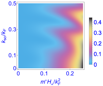
Figure 2: (Color online.) The magnetoconductance difference, $U_{ii}-U_{i}$, calculated for $k_{\rm F}d=20$, as function of the spin-orbit coupling ($k_{\rm so}$) measured in units of the Fermi wave vector, and the Zeeman energy, measured in units of $k^{2}_{\rm F}/m^{\ast}$. The oscillations shown are due to the term $\propto\cos(\alpha)$ of $U_{ii}$; $\alpha=(k_{+}-k_{-})d$.

The spin-current vector ${\bf W}$ in this configuration is conveniently separated into components ${\bf W}_{\rm perp}$ along $\hat{\bf q}_{+}\times\hat{\bf q}_{-}\parallel\hat{\bf h}_{\rm so}\times{\bf H}_{\perp}$, and ${\bf W}_{\rm plane}$ in the $\{\hat{\bf q}_{+},\hat{\bf q}_{-}\}$ (or $\{\hat{\bf h}_{\rm so},{\bf H}_{\perp}\})-$plane. The magnitudes of those are sup

$$W_{\rm perp}=2A_{+}A_{-}|\sin(\alpha)\hat{\bf q}_{+}\times\hat{\bf q}_{-}|\ ,$$

$$W_{\rm plane}=2\Big{|}(A^{2}_{+}-A^{2}_{-})^{2}+2A_{+}A_{-}[1-\hat{\bf q}_{+}\cdot\hat{\bf q}_{-}]$$

$$\times\Big{(}A_{+}A_{-}+\cos(\alpha)(A^{2}_{+}+A^{2}_{-})+A_{+}A_{-}\cos^{2}(\alpha)\Big{)}\Big{|}^{1/2}\ .$$ (23)

The magnitude of ${\bf W}_{\rm plane}$ and ${\bf W}_{\rm perp}$ are displayed in Figs. 3 and 4, respectively. The (almost) double periodicity in Fig. 4 as compared with Fig. 3 appears since $|{\bf W}_{\rm perp}|$ is proportional to $\sin(\alpha)$.

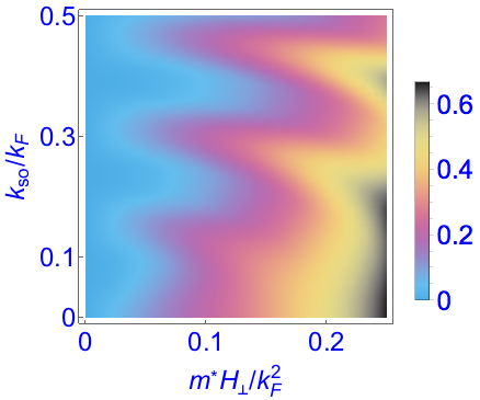
Figure 3: (Color online.) The magnitude of the spin current along ${\bf W}_{\rm plane}$ with the same parameters as in Fig. 2.

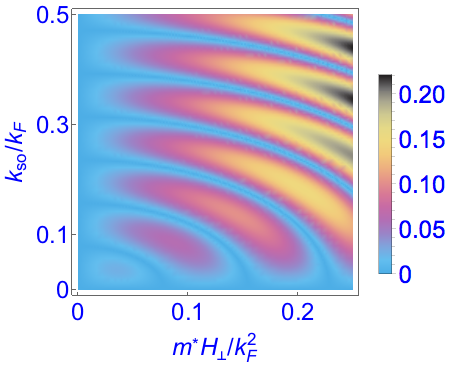
Figure 4: (Color online.) The magnitude of the spin current ${\bf W}_{\rm perp}$ with the same parameters as in Fig. 2.

In summary, we have shown that a net amount of charge and magnetic moment per unit time is transferred through a biased spin-orbit active weak-link from a source to a drain electrode. Electrons enter and leave the weak-link wire at injection points, whose small volumes are characterized by the cross-section radius $r_{0}$ of the wire. Assuming the volumes of the electrodes are much larger than these injection volumes, and if the system is part of a closed electrical circuit, the density of the injected electrons, $\delta n(r)$, and the density of the associated magnetic moment, $M(r)$, will decrease with the distance $r$ from the ends of the wire due to a geometrical spreading effect, $\delta n(r)/\delta n(r_{0})\,,\,\,M(r)/M(r_{0})\propto\left(r_{0}/r\right)^{x}$, where $x=2$ ($x=1$) in the ballistic (diffusive) transport regime JETP ; LTP . The injected magnetization can be measured, e.g., by a properly-positioned SQUID, or by a magnetic-resonance force microscope. In an open electrical circuit, the injection of magnetic moments will lead to a finite magnetization, proportional to the bias voltage, in the entire volume of each electrode.

- (1) S. A. Wolf, D. D. Awschalom, R. A. Buhrman, J. M. Daughton, S. von Molnár, M. L. Roukes, A. Y. Chtchelkanova, and D. M. Treger, Spintronics: a spin-based electronics vision for the future, Science 294, 1488 (2001).
- (2) I. Žutić, J. Fabian, and S. Das Sarma, Spintronics: fundamentals and applications, Rev. Mod. Phys. 76, 323 (2004).
- (3) M. Kohda and J. Nitta, Enhancement of spin-orbit interaction and the effect of interface diffusion in quaternary InGaAsP/InGaAs heterostructures, Phys. Rev. B 81, 115118 (2010).
- (4) R. Winkler, Spin-Orbit Coupling Effects in Two-Dimensional Electron and Hole Systems, (Springer-Verlag, Berlin, 2003).
- (5) A. Manchon, H. C. Koo, J. Nitta, S. M. Frolov, and R. A. Duine, New Perspectives for Rashba Spin-Orbit Coupling, Nat. Mater. 14, 871 (2015).
- (6) E. I. Rashba, Properties of semiconductors with an extremum loop .1. Cyclotron and combinational resonance in a magnetic field perpendicular to the plane of the loop, Fiz. Tverd. Tela (Leningrad) 2, 1224 (1960) [Sov. Phys. Solid State 2, 1109 (1960)]; Y. A. Bychkov and E. I. Rashba, Oscillatory effects and the magnetic susceptibility of carriers in inversion layers, J. Phys. C 17, 6039 (1984).
- (7) J. Nitta, T. Akazaki, H. Takayanagi, and T. Enoki, Gate Control of Spin-Orbit Interaction in an Inverted In0.53Ga0.47As/In0.52Al0.48As Heterostructure, Phys. Rev. Lett. 78, 1335 (1997).
- (8) Y. Sato, T. Kita, S. Gozu, and S. Yamada, Large spontaneous spin splitting in gate-controlled two-dimensional electron gases at normal In0.75Ga0.25As/In0.75Al0.25As heterojunctions, J. Appl. Phys. 89, 8017 (2001).
- (9) A. J. A. Beukman, F. K. de Vries, J. van Veen, R. Skolasinski, M. Wimmer, F. Qu, D. T. de Vries, B. M. Nguyen, W. Yi, A. A. Kiselev, M. Sokolich, M. J. Manfra, F. Nichele, C. M. Marcus, and L. P. Kouwenhoven, Spin-orbit interaction in a dual gated InAs/GaSb quantum well, Phys. Rev. B 96, 241401 (2017).
- (10) Other types of SOI, e.g. the Dresselhaus SOI [G. Dresselhaus, Spin-Orbit Coupling Effects in Zinc Blende Structures, Phys. Rev. 100, 580 (1955)], or those resulting from strains in the wire [M. S. Rudner and E. I. Rashba, Spin relaxation due to deflection coupling in nanotube quantum dots, Phys. Rev. B 81, 125426 (2010); K. Flensberg and C. M. Marcus, Bends in nanotubes allow electric spin control and coupling, Phys. Rev. B 81, 195418 (2010), G. A. Steele, F. Pei, E. A. Laird, J. M. Jol, H. B. Meerwaldt, and L. P. Kouwenhoven, Large spin-orbit coupling in carbon nanotubes, Nature Comm. 2584, (2013)], yield similar effects, with other directions of the effective SOI magnetic field around which the spins rotate.
- (11) S. Datta and B. Das, Electronic analog of the electro‐optic modulator, Appl. Phys. Lett. 56, 665 (1990).
- (12) J. H. Bardarson, A proof of the Kramers degeneracy of transmission eigenvalues from antisymmetry of the scattering matrix, J. Phys. A: Math. Theor. 41, 405203 (2008).
- (13) A. G. Aronov and Y. B. Lyanda-Geller, Spin-Orbit Berry Phase in Conducting Rings, Phys. Rev. Lett. 70, 343 (1993).
- (14) A. Aharony, Y. Tokura, G. Z. Cohen, O. Entin-Wohlman, and S. Katsumoto, Filtering and analyzing mobile qubit information via Rashba-Dresselhaus-Aharonov-Bohm interferometers, Phys. Rev. B 84, 035323 (2011) and references therein.
- (15) H. Saarikoski, A. A. Reynoso, J. P. Baltanás, D. Frustaglia, and J. Nitta, Spin interferometry in anisotropic spin-orbit fields, Phys. Rev, B 97, 125423 (2018); see also F. Nagasawa, A. A. Reynoso, J. P. Baltanás, D. Frustaglia, H. Saarikoski, and J. Nitta, Gate-controlled anisotropy in Aharonov-Casher spin interference, arXiv:1803.11371.
- (16) Y. V. Pershin, J. A. Nesteroff, and V. Privman, Effect of spin-orbit interaction and in-plane magnetic field on the conductance of a quasi-one-dimensional system, Phys. Rev. B 69, 121306(R) (2004).
- (17) C. H. L. Quay, T. L. Hughes, J. A. Sulpizio, L. N. Pfeiffer, K. W. Baldwin, K. W. West, D. Goldhaber-Gordon, and R. de Picciotto, Observation of a one-dimensional spin-orbit gap in a quantum wire, Nat. Phys. 6, 336 (2010).
- (18) C. Tang, Y. Yu, N. R. Abdullah, and V. Gudmundsson, Transport signatures of top-gate bound states with strong Rashba-Zeeman effect, Phys. Lett. A 381, 3960 (2017).
- (19) Y. Oreg and O. Entin-Wohlman, Transmissions through low-dimensional mesoscopic systems subject to spin-orbit scattering, Phys. Rev. B 46, 2393 (1992).
- (20) This feature distinguishes the present geometry from the devices based on Aharonov-Bohm interferometers where the Zeeman energy is compared to the Fermi energy.
- (21) Y. Aharonov and A. Casher, Topological quantum effects for neutral particles, Phys. Rev. Lett. 53, 319 (1984).
- (22) We note that is related to the Rashba parameter : . The full strength of the spin-orbit coupling includes the sine of the angle between and the direction of motion, i.e., [see Eq. (6)]. In earlier papers (e.g. Ref. revRashba, ) we did not include this factor.
- (23) R. I. Shekhter, O. Entin-Wohlman, M. Jonson, and A. Aharony, Rashba splitting of Cooper pairs, Phys. Rev. Lett. 116, 217001 (2016) and supplementary material there.
- (24) T. Jonckheere, G. I. Japaridze, T. Martin, and R. Hayn, Transport through a band insulator with Rashba spin-orbit coupling: Metal-insulator transition and spin-filtering effects, Phys. Rev. B 81, 16543 (2010).
- (25) T. V. Shahbazyan and M. E. Raikh, Low field anomaly in 2D hopping magnetoresistance caused by spin-orbit term in the energy spectrum, Phys. Rev. Lett. 73, 1408 (1994).
- (26) See Supplemental Material at http://link.aps.org/supplemental for a detailed derivation.
- (27) are real and positive as we assume the Zeeman energy to be smaller than the fermi energy, .
- (28) We consider those two quantities in the left lead; the ones corresponding to the right lead are derived similarly. They have opposite signs to those of the left lead.
- (29) The denominators in Eqs. (18) and (19) vanish when the Zeeman energy approaches the Fermi energy. However, our perturbative calculation requires small tunneling matrix elements, and therefore these equations can be used only when the Zeeman energy is significantly smaller than the Fermi energy.
- (30) I. O. Kulik, R. I. Shekhter, and A. G. Shkorbatov, Point-contact spectroscopy of electron-phonon coupling in metals with a small electron mean free path, Sov. Phys. JETP 54, 1130 (1981); Eqs. (2.11), (2.12), and (3.3 - 3.5).
- (31) R. I. Shekhter and I. O. Kulik, Spectroscopy of phonons in heterocontacts, Sov. J. Low Temp. Phys. 9, 22 (1983); The Introduction and Section 1.