Age-Optimal Trajectory Planning for UAV-Assisted Data Collection

Abstract

Unmanned aerial vehicle (UAV)-aided data collection is a new and promising application in many practical scenarios. In this work, we study the age-optimal trajectory planning problem in UAV-enabled wireless sensor networks, where a UAV is dispatched to collect data from the ground sensor nodes (SNs). The age of information (AoI) collected from each SN is characterized by the data uploading time and the time elapsed since the UAV leaves this SN. We attempt to design two age-optimal trajectories, referred to as the Max-AoI-optimal and Ave-AoI-optimal trajectories, respectively. The Max-AoI-optimal trajectory planning is to minimize the age of the ‘oldest’ sensed information among the SNs. The Ave-AoI-optimal trajectory planning is to minimize the average AoI of all the SNs. Then, we show that each age-optimal flight trajectory corresponds to a shortest Hamiltonian path in the wireless sensor network where the distance between any two SNs represents the amount of inter-visit time. The dynamic programming (DP) method and genetic algorithm (GA) are adopted to find the two different age-optimal trajectories. Simulation results validate the effectiveness of the proposed methods, and show how the UAV’s trajectory is affected by the two AoI metrics.

I Introduction

Unmanned aerial vehicles (UAVs) have attracted a lot of attentions in both academia and industry [1]. Thanks to its fully controllable mobility, the UAV can be employed to collect the sensed data from the ground sensor nodes (SNs) as a mobile data collector. The UAV can move very close to each SN and communicate with it via low-altitude line-of-sight (LoS) communication links [2]. Hence, the UAV-assisted data collection can save the transmission energy of each SN, and prolong the lifetime of wireless sensor networks.

The efficiency of data collection and design of UAV’s trajectory have been studied recently for UAV-assisted wireless sensor networks [3, 4, 5]. In [3], considering the fairness between the cluster heads that communicate with the UAV directly, Abdulla et al. formulated the energy efficiency maximization problem in UAV-aided data collection as a potential game. The impacts of the UAV’s trajectory on the adaptive modulation scheme were also discussed. Say et al. proposed in [4] a UAV-assisted data gathering framework for wireless sensor networks, where the UAV is used as a relay to collect the sensed data from the SNs. Inside the UAV’s coverage area, the sensors are divided into different frames according to their locations and assigned with different transmission priorities to reduce the packet loss. The authors of [5] studied the joint optimization of the SNs’ wake-up schedule and UAV’s trajectory in UAV-enabled wireless sensor networks for reliable and energy-efficient data collection. The successive convex optimization method was applied to find a sub-optimal UAV’s trajectory. It is shown in these works that the UAV’s trajectory greatly affects the efficiency of data collection.

On the other hand, the freshness of the sensed information is very crucial in delay-sensitive applications. The freshness is a new and important metric, referred to as the age of information (AoI) or status age, which is defined as the amount of time elapsed since the instant at which the freshest delivered update takes place [6]. Most existing works focused on analyzing or optimizing the AoI-based schedule or transmission [6, 7, 8]. In [6], the age-optimal throughput region was derived for the first-come-first-served M/M/1 queueing system. The status age was derived for status updates randomly generated and transmitted in a cloud-based network in [7]. Sun et al. studied the optimal control policy of information updates in a communication system and proposed the zero-wait policy to keep the data fresh [8]. Efficient algorithms were developed to find the optimal update policy in the constrained semi-Markov decision framework.

Motivated by the above works, we are interested in investigating the impacts of AoI metrics on the design of UAV-assisted data collection. In this work, we study the age-optimal trajectory planning problem in UAV-enabled wireless sensor networks. The UAV takes off from the data center, collects the sensed data from all the SNs sequentially and delivers them to the data center for information processing when it flies back to it. The AoI of each SN is equal to the amount of time elapsed from the instant at which the information is sensed to the instant at which the information is delivered to the data center. It is easy to see that the UAV’s trajectory has a great impact on the AoI of each SN. Particularly, we define two different AoI metrics, i.e., the maximum AoI and average AoI of SNs. Accordingly, the UAV’s optimal trajectories are referred to as the Max-AoI-optimal and Ave-AoI-optimal trajectories, respectively. Through theoretical analysis, we show that the Max-AoI-optimal trajectory is exactly a shortest Hamiltonian path while the Ave-AoI-optimal one is a stage-weighted shortest Hamiltonian path in the wireless sensor network. Then, we adopt the dynamic programming (DP) approach to find the two age-optimal trajectories recursively. The computational complexity of DP is rather high as the network size increases. For large-scale wireless sensor networks, we develop a genetic algorithm (GA) to intelligently search the near optimal trajectories. Simulation results show the importance of the two AoI metrics in the design of the UAV’s trajectory.

II System Model

Fig. 1: An illustrative model of UAV-enabled data collection: The UAV flies following a trajectory $v_{0}\rightarrow v_{1}\rightarrow v_{4}\rightarrow v_{3}\rightarrow v_{5}\rightarrow v_{2}\rightarrow v_{0}$, collects the latest sensing information from each SN $v_{i}$ ($i=1,\cdots,5$), and flies back to the data center $v_{0}$.

As shown in Fig. 1, we consider a UAV-enabled wireless sensor network in which a UAV is dispatched to collect data from $M$ SNs, denoted by $\mathcal{V}=\left\{v_{1},\cdots,v_{M}\right\}$, and then flies back to the data center $v_{0}$ for data analysis. The network can be described by a complete graph $G=(\mathcal{V}^{+},\,\mathcal{E})$, where $\mathcal{V}^{+}=\left\{v_{0}\right\}\bigcup\mathcal{V}$ denotes the set of all the nodes including the data center, and $\mathcal{E}=\{(v_{i},v_{j})\,|v_{i},v_{j}\in\mathcal{V},\,i\neq j\}$ denotes the set of all the edges connecting any two nodes. For ease of exposition, we denote by $\mathcal{N}_{m}=\{v_{i}|(v_{i},v_{m})\in\mathcal{E},v_{i}\in\mathcal{V}^{+}\}$ the set of the neighboring nodes of node $v_{m}$. Each edge $(v_{i},v_{j})$ has an associated non-negative weight $d_{i,j}$, indicating the distance between nodes $v_{i}$ and $v_{j}$, i.e., $d_{i,j}=\|\bm{s}_{i}-\bm{s}_{j}\|$, where $\bm{s}_{i}=[x_{i},y_{i}]\in\mathbb{R}^{2}$ is the location of node $v_{i}$.

To collect the information, the UAV takes off from the data center $v_{0}$, flies to collect the information from all the $M$ nodes following a prescheduled trajectory, and lands at the data center after completing the job. The UAV flies at a fixed altitude $h$ and maintains a constant flight velocity, denoted by $V$. Except the start/end point $v_{0}$, the trajectory is supposed to contain the sequence of the non-repeating nodes, like $v_{0}\rightarrow v_{(1)}\rightarrow v_{(2)}\rightarrow\cdots\rightarrow v_{(M)}\rightarrow v_{(M+1)}=v_{0}$, where $v_{(i)}\in\mathcal{V}$ denotes the $i$-th node in the trajectory. Here, the trajectory vector $\bm{u}=[v_{(1)},v_{(2)}\cdots,v_{(M)}]$ specifies one permutation of the node set $\mathcal{V}$.

When the UAV flies to and hovers above node $v_{(i)}$, it establishes a line-of-sight communication link immediately with this node. Node $v_{(i)}$ samples its sensing information, packs it in a data packet of length $L_{(i)}^{p}$ with timestamp $T_{i}$, and transmits the tagged packet to the UAV. Without loss of generality, we assume that the UAV takes off at time $T_{0}=0$. The channel power gain of the LOS link from the node to the UAV can be modeled as $g=\beta h^{-2}$, where $\beta$ denotes the channel gain at the reference distance [2]. When the node transmits at a constant power $P_{(i)}$, its uploading data rate over the LOS link can be expressed as

$$R_{(i)}=B\log_{2}\left(1+\frac{g\cdot P_{(i)}}{\sigma^{2}}\right)=B\log_{2}\left(1+\frac{\beta}{h^{2}\sigma^{2}}P_{(i)}\right),$$ (1)

where $B$ denotes the system bandwidth, and $\sigma^{2}$ denotes the noise power at the UAV receiver. Assuming that the sensing time is very small and negligible, the data collection time at node $v_{(i)}$ can be evaluated as $t_{(i)}^{tx}=L_{(i)}^{p}/R_{(i)}$. The set of SNs that have been visited by the UAV till now is denoted by $\mathcal{C}_{i}=\{v_{(1)},\cdots,v_{(i)}\}$. Then, the UAV flies directly to the next node $v_{(i+1)}$ in the trajectory and continues the data collecting job. After visiting all the nodes, the UAV returns back to the data center at time $T_{(M+1)}$ for data analysis.

We use $X_{i}(t)$ to track the age of the information collected from the $i$-th node $v_{(i)}$ in the flight trajectory at time $t$. When $t<T_{i}$, $X_{i}(t)=0$, since node $v_{(i)}$ has not been visited at this time and its information has not been sampled [6]. Otherwise, $X_{i}(t)=t-T_{i}$. Hence, the information age of node $v_{(i)}$ is given by

$$X_{i}(t)=\left(t-T_{i}\right)^{+},\quad i=1,2,\cdots,M,$$ (2)

where $(x)^{+}=\max\{0,x\}.$ At instant $t=T_{i+1}$, the AoI collected from node $v_{(i)}$ is equal to

$$X_{i}(T_{i+1})\triangleq\eta_{(i),(i+1)}=t_{(i)}^{tx}+t_{(i),(i+1)}^{flight},$$ (3)

where $t_{(i),(i+1)}^{flight}=V^{-1}d_{(i),(i+1)}$ denotes the flight time of the UAV from node $v_{(i)}$ to node $v_{(i+1)}$. Here, $\eta_{(i),(i+1)}$ indicates the amount of time elapsed between two data collection actions at node $v_{(i)}$ and node $v_{(i+1)}$. When getting back to the data center at time $T_{(M+1)}$, the UAV has visited all the SNs and collected $M$ data packets including sensing information with different ages, given by

$$X_{i}(T_{(M+1)})=T_{(M+1)}-T_{i}=\sum_{k=i}^{M}\eta_{(k),(k+1)},$$ (4)

which is totally determined by the trajectory $\bm{u}$ and hence can be expressed as a function of the trajectory $\bm{u}$, i.e., $X_{i}(T_{(M+1)})=X_{i}(\bm{u})$. Similarly, the average age of the sensing information can be computed as

$$\overline{X}(T_{(M+1)})=\overline{X}(\bm{u})=\frac{1}{M}\sum_{i=1}^{M}X_{i}(\bm{u}).$$ (5)

In this work, we attempt to design two age-optimal flight trajectories for UAV-assisted data collection. One is to minimize the age of the ‘oldest’ sensing information among the SNs. The other is to minimize the average age of the sensing information. In particular, we formulate two combinatorial optimization problems as follows:

$$\mathcal{P}_{1}:\quad\min_{\bm{u}}\,\max_{i\in\{1,\cdots,M\}}\left\{X_{i}(\bm{u})\right\}$$ (6)

and

$$\mathcal{P}_{2}:\quad\min_{\bm{u}}\,\overline{X}(\bm{u}).$$ (7)

The optimal solutions to Problems $\mathcal{P}_{1}$ and $\mathcal{P}_{2}$ are denoted by $\bm{u}_{max}^{*}$ and $\bm{u}_{ave}^{*}$, referred to as the optimal maximum-age-of-information (Max-AoI-optimal) trajectory and the optimal average-age-of-information (Ave-AoI-optimal) trajectory, as discussed below.

III AoI-Optimal Trajectory Planning

By analyzing the properties of Problems $\mathcal{P}_{1}$ and $\mathcal{P}_{2}$, we show that the Max-AoI-optimal and Ave-AoI-optimal flight trajectories are actually two shortest Hamiltonian paths.

III-A Max-AoI-optimal Trajectory

Among all the SNs, the first node $v_{(1)}$ in the trajectory $\bm{u}$ always experiences the largest AoI, as presented in the following lemma.

Lemma 1.

For any flight trajectory $\bm{u}$, we have

$$X_{1}(\bm{u})>X_{2}(\bm{u})>\cdots>X_{M}(\bm{u}).$$ (8)

From Lemma 1, Problem $\mathcal{P}_{1}$ is equivalent to

$$\mathcal{P}_{1}^{{}^{\prime}}:\quad\min_{\bm{u}}\quad X_{1}(\bm{u}).$$ (9)

Accordingly, the optimal value of Problem $\mathcal{P}_{1}^{{}^{\prime}}$ is denoted by $X_{1}^{*}=X_{1}(\bm{u}_{max}^{*})$.

Theorem 2.

The Max-AoI-optimal trajectory is a shortest Hamiltonian path that where the distance between any two nodes $v_{i}$ and $v_{j}$ is equal to $\eta_{i,j}$.

Proof:

Notice that the length of the flight trajectory is equal to

$$X_{1}(\bm{u})=\sum_{k=1}^{M}\eta_{(i),(i+1)}.$$ (10)

Thus, solving Problem $\mathcal{P}_{1}^{{}^{\prime}}$ is equivalent to finding a shortest Hamiltonian path $\bm{u}_{max}^{*}$ that starts from node $v_{(1)}$ and visits all the other nodes exactly once before going back to the data center $v_{0}$. The AoI of node $v_{(1)}$ is equal to the length of the Hamiltonian path $X_{1}(\bm{u})$, which is to be minimized. ∎

In graph theory, a Hamiltonian path is a path in an undirected or directed graph that visits each vertex exactly once [9]. There exists a Hamiltonian path in the complete graph $G$. Hence, to find the Max-AoI-optimal flight trajectory, we shall find a shortest Hamiltonian path that visits all the SNs $\{v_{i}\}$ $(i=1,\cdots,M)$ exactly once and goes back to the data center $v_{0}$. In this scenario, the time parameters $\{\eta_{i,j}\}$ $(\forall i,j\in\mathcal{V}^{+})$ are treated as the distances between any two nodes.

III-B Ave-AoI-optimal Trajectory Planning

Similarly, we analyze the average age of the sensing information $\overline{X}(\bm{u})$ and discuss the Ave-AoI-optimal trajectory planning problem $\mathcal{P}_{2}$.

Lemma 3.

The average AoI given by (5) can be re-expressed as

$$\overline{X}(\bm{u})=\sum_{i=1}^{M}\frac{i}{M}\cdot\eta_{(i),(i+1)}.$$ (11)

For ease of exposition, we define the weighted AoI collected from node $v_{(i)}$ to node $v_{(M)}$ along the trajectory $\bm{u}$ as

$$\overline{X}_{i}(\bm{u})=\sum_{k=i}^{M}\frac{k}{M}\cdot\eta_{(k),(k+1)},$$ (12)

which satisfies

$$\overline{X}_{i}(\bm{u})>\overline{X}_{j}(\bm{u})\quad\forall i<j.$$ (13)

Thus, the average information age is obtained as $\overline{X}(\bm{u})=\overline{X}_{1}(\bm{u})$. Thus, Problem $\mathcal{P}_{2}$ is equivalent to

$$\mathcal{P}_{2}^{{}^{\prime}}:\quad\min_{\bm{u}}\quad\overline{X}_{1}(\bm{u}).$$ (14)

The Ave-AoI-optimal trajectory is the optimal solution of $\mathcal{P}_{2}^{{}^{\prime}}$ and the optimal value is denoted by $\overline{X}_{1}^{*}=\overline{X}_{1}(\bm{u}_{ave}^{*})$ accordingly.

Theorem 4.

The Ave-AoI-optimal trajectory is a stage-weighted shortest Hamiltonian path where the stage-weighted distance between node $v_{(k)}$ and $v_{(k+1)}$ is equal to $\frac{k}{M}\cdot\eta_{(k),(k+1)}$.

Proof:

For any trajectory $\bm{u}$, the average AoI can be viewed as the stage-weighted length of the trajectory, i.e.,

$$\overline{X}_{1}(\bm{u})=\sum_{k=1}^{M}\frac{k}{M}\cdot\eta_{(k),(k+1)},$$ (15)

where $\frac{k}{M}$ is the weight. Specifically, the distance between nodes $v_{(k)}$ and $v_{(k+1)}$ is equal to $\frac{k}{M}\cdot\eta_{(k),(k+1)}$. Thus, solving Problem $\mathcal{P}_{2}^{{}^{\prime}}$ is equivalent to finding a stage-weighted shortest Hamiltonian path $\bm{u}_{ave}^{*}$ that starts from node $v_{(1)}$ and visits all the other nodes exactly once before going back to the data center $v_{0}$. From (15), the minimum average AoI is equal to the stage-weighted length of the shortest Hamiltonian path $\bm{u}_{ave}^{*}$. ∎

In this theorem, we show that the Ave-AoI-optimal trajectory can also be regarded as a shortest Hamiltonian path in the wireless sensor network. However, the distance between two consecutive nodes $v_{(k)}$ and $v_{(k+1)}$ in the trajectory is equal to the product of the factor $\frac{k}{M}$ and the time parameter $\eta_{(k),(k+1)}$. In the sequel, we discuss the algorithm design problem for AoI-Optimal trajectory planning.

IV Algorithm Design for AoI-Optimal Trajectory Planning

In this part, we discuss how to find the Max-AoI-optimal and Ave-AoI-optimal trajectories using methods of DP and genetic algorithm (GA), respectively.

Algorithm 1 DP-based age-optimal trajectory planning

1:  Input: the network topology $G=(\mathcal{V}^{+},\,\mathcal{E})$, and the system parameters $(V,h,\beta,B,P_{m},\sigma^{2})$ for all $v_{m}\in\mathcal{V}$.

2:  Calculate the elapsed time of data collection between any two nodes $\eta_{i,j}$ (c.f. (3)) for all $i\neq j$, $v_{i},v_{j}\in\mathcal{V}^{+}$;

3:  for $i=1:M$ do

4:     for $S\subseteq\mathcal{V}-\{v_{i}\}$ do

5:        Calculate the minimum path cost $f(i,S)$ (or $g(i,S)$) according to (16) (or (18));

6:     end for

7:  end for

8:  Calculate the minimum AoI as $X_{1}^{*}$ (or $\overline{X}_{1}^{*}$) by (17) (or (19));

9:  Find the optimal node $v_{(1)}^{*}=\arg\min_{v_{i}\in\mathcal{V}}f(i,\mathcal{V}-\{v_{i}\})$ (or $v_{(1)}^{*}=\arg\min_{v_{i}\in\mathcal{V}}g(i,\mathcal{V}-\{v_{i}\})$) that is firstly visited;

10:  Trace back to find the optimal trajectory $\bm{u}_{max}^{*}$ (or $\bm{u}_{ave}^{*}$) starting with node $v_{(1)}^{*}$ and ending with node $v_{0}$;

11:  Output: the optimal trajectory $\bm{u}_{max}^{*}$ (or $\bm{u}_{ave}^{*}$).

IV-A DP-based AoI-Optimal Trajectory Planning

i) The Max-AoI-optimal Case: We first apply the DP method to find the Max-AoI-optimal flight trajectory in the wireless sensor network. Let $f(i,S)$ $(v_{i}\notin S\subset\mathcal{V})$ denote the minimum cost of the path starting from node $v_{i}$, passing all the vertices in the set $S$ exactly once and going back to the data center $v_{0}$. The minimum path cost $f(i,S)$ can be expressed in a recursive form:

$$f(i,S)=\begin{cases}\eta_{i,0},&S=\emptyset,\\ \min\limits_{v_{k}\in S}\left\{\eta_{i,k}+f(k,S-\{k\})\right\},&S\neq\emptyset.\end{cases}$$ (16)

The Max-AoI-optimal trajectory is exactly the shortest Hamiltonian path that achieves the minimum cost

$$X_{1}^{*}=\min_{v_{i}\in\mathcal{V}}f(i,\mathcal{V}-\{v_{i}\}),$$ (17)

where the cost function $f(i,\mathcal{V}-\{v_{i}\})$ is calculated by (16).

ii) The Ave-AoI-optimal Case: Similarly, we show that the Ave-AoI-optimal trajectory can also be found using the DP method. Let $g(i,S)$ $(v_{i}\notin S)$ denote the minimum weighted cost of the path starting from node $v_{i}$, passing all the vertices in the set $S$ exactly once and returning back to the data center $v_{0}$. To find the stage-weighted shortest Hamiltonian path, we express the minimum weighted path cost $g(i,S)$ as:

$$g(i,S)=\begin{cases}\eta_{i,0},&S=\emptyset,\\ \min\limits_{v_{k}\in S}\left\{(1-\frac{|S|}{M})\eta_{i,k}+g(k,S-\{k\})\right\},&S\neq\emptyset.\end{cases}$$ (18)

where $|S|$ denotes the cardinality of the set $S$, i.e., the number of elements in $S$. Here, $|S|$ is used to indicate how many nodes remain unvisited. Accordingly, $1-\frac{|S|}{M}$ can be used to represent the stage weight. Therefore, the Ave-AoI-optimal trajectory is also the ‘shortest’ Hamiltonian path that obtains the minimum path cost as

$$\overline{X}_{1}^{*}=\min_{v_{i}\in\mathcal{V}}g(i,\mathcal{V}-\{v_{i}\}),$$ (19)

where the cost function $g(i,\mathcal{V}-\{v_{i}\})$ is calculated by (18) iteratively.

iii) Algorithm Design: According to the above discussions, we propose a DP based algorithm, i.e., Algorithm 1, to find the two AoI-optimal trajectories. In particular, we first calculate the distance $\eta_{i,j}$ between any two nodes $v_{i}$ and $v_{j}$ by (3). To find the Max-AoI-optimal trajectory, we calculate the minimum path costs $f(i,S)$ recursively by (16) for each node $v_{i}\in\mathcal{V}$ and all the subsets $S\subseteq\mathcal{V}-\{v_{i}\}$. The minimum path cost $f(i,S)$ and the node $\tau\in S$ being visited exactly after node $v_{i}$ are recorded in a table. From (17), the minimum AoI as $X_{1}^{*}$ is found by comparing the minimum path costs $f(i,\mathcal{V}-\{v_{i}\})$ for all $v_{i}\in\mathcal{V}$. Accordingly, the optimal node firstly visited by the UAV is marked as $v_{(1)}^{*}$. The shortest Hamiltonian path $\bm{u}_{max}^{*}$ can be found by tracing back the data stored in the table. Using the DP algorithm, the Ave-AoI-optimal trajectory $\bm{u}_{ave}^{*}$ can be found in the same way. Notice that the minimum weighted path costs $g(i,S)$ (c.f. (18)) rather than the path costs $f(i,S)$ shall be calculated and recorded.

In this way, we can find the Max-AoI-optimal and Ave-AoI-optimal trajectories using Algorithm 1. The computational complexity of the DP method is about $O(M\cdot 2^{M})$, which becomes intolerable when the number of nodes $M$ is large. To deal with this issue, we develop a genetic algorithm (GA) to solve the AoI-optimal trajectory planning problems $\mathcal{P}_{1}^{{}^{\prime}}$ and $\mathcal{P}_{2}^{{}^{\prime}}$ in the sequel.

IV-B GA-based AoI-Optimal Trajectory Planning

Algorithm 2 GA-based age-optimal trajectory planning

1:  Input: the network topology $G=(\mathcal{V}^{+},\,\mathcal{E})$, the data collecting time matrix $\bm{\eta}=[\eta_{i,j}]$, and the GA related parameters $\{N_{c},N_{g},\alpha,\gamma_{c},\gamma_{m}\}$;

2:  Step 1: Create an initial population of $N_{c}$ chromosomes, and set the generation index as $n=0$;

3:  Step 2: Evaluate the normalized fitness of each chromosome $\bm{u}$ by substituting $l(\bm{u})=X_{1}(\bm{u})$ or $l(\bm{u})=\overline{X}_{1}(\bm{u})$ into (20);

4:  Step 3: Randomly choose the parent chromosomes via proportional selection according to the threshold $\gamma_{c}$; Create offsprings from the selected parent chromosomes using partially mapped crossover operation; Apply the mutation operations on the current population of $N_{c}$ chromosomes with probability $\gamma_{m}$;

5:  Step 4: Generate a new population of $N_{c}$ chromosomes by replacing old chromosomes with new ones, and increase the generation index $n$ by one, i.e., $n=n+1$; The procedure goes to Step 2 if $n<N_{g}$; Otherwise, it is terminated.

6:  Step 5: Calculate the fitness of each chromosome $\bm{u}\in\mathcal{C}$, and find the optimal trajectory $\bm{u}_{max}^{*}=\arg\max\limits_{\bm{u}\in\mathcal{C}}l(\bm{u})=X_{1}(\bm{u})$ (or $\bm{u}_{ave}^{*}=\arg\max\limits_{\bm{u}\in\mathcal{C}}l(\bm{u})=\overline{X}_{1}(\bm{u})$);

7:  Output: the optimal trajectory $\bm{u}_{max}^{*}$ (or $\bm{u}_{ave}^{*}$).

In Algorithm 2, we present the GA-based AoI-optimal trajectory planning algorithm which consists of the following several steps.

Step 1: we create an initial population of $N_{c}$ chromosomes, denoted by a set $\mathcal{C}$. Each chromosome represents a feasible Hamiltonian path $\bm{u}$ in the wireless sensor network. The generation index $n$ is set as zero.

Step 2: we evaluate the normalized fitness of each chromosome $\bm{u}$ as

$$\phi(\bm{u})=\left(1-\frac{l(\bm{u})-l_{min}(\mathcal{C})}{l_{max}(\mathcal{C})-l_{min}(\mathcal{C})+\epsilon}\right)^{\alpha},$$ (20)

where $l(\bm{u})$ denotes the length of path $\bm{u}$ that is equal to the maximum age $X_{1}(\bm{u})$ or the maximum average age $\overline{X}_{1}(\bm{u})$, $l_{max}(\mathcal{C})=\max_{\bm{u}\in\mathcal{C}}l(\bm{u})$ and $l_{min}(\mathcal{C})=\min_{\bm{u}\in\mathcal{C}}l(\bm{u})$ are the maximum length and the minimum length of all the paths in the set $\mathcal{C}$, $\alpha$ is an acceleration factor that is larger than one, and $\epsilon$ is a very small value used for adjustment.

Step 3: we apply the selection, crossover and mutation operations on the population of $N_{c}$ chromosomes. Firstly, we randomly choose the parent chromosomes via proportional selection for mating. This means that in accordance with shorter Hamiltonian paths, the chromosomes with higher fitness have a larger probability of being selected. Specifically, the chromosome is selected if its fitness value is larger than a threshold $\gamma_{c}$. The set of the selected chromosomes is denoted by $N_{c}^{{}^{\prime}}$. Secondly, we randomly choose $\lfloor\frac{N_{c}^{{}^{\prime}}}{2}\rfloor$ pairs of parents to create offsprings using partially mapped crossover operation. By marking two random cut points on a pair of parent paths, the nodes between cut points are exchanged between the two paths to create two offspring paths. The repetitive nodes between the offspring paths are then exchanged to produce two offspring Hamiltonian paths. Thirdly, we apply mutation operation on each chromosome with probability $\gamma_{m}$. That is, two nodes of a path $\bm{u}$ are randomly selected and exchanged several time.

Step 4: we generate a new population of $N_{c}$ chromosomes by replacing a proportion of old chromosomes with new ones. Thus, the number of generations $n$ is increased by one. The procedure is terminated if the number of generations reaches its maximum value $N_{g}$, i.e., $n=N_{g}$. Otherwise, the process goes to Step 2 and repeats.

Step 5: we calculate the fitness of each chromosome in the final generation, and set the chromosome with the maximum fitness as the optimal flight trajectory, i.e., $\bm{u}_{max}^{*}=\arg\max\limits_{\bm{u}\in\mathcal{C}}l(\bm{u})=X_{1}(\bm{u})$ (or $\bm{u}_{ave}^{*}=\arg\max\limits_{\bm{u}\in\mathcal{C}}l(\bm{u})=\overline{X}_{1}(\bm{u})$);

In this way, we develop the GA-based algorithm to find the Max-AoI-optimal and Ave-AoI-optimal trajectories.

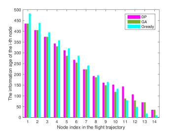
Figure 2: The minimum AoI $X_{i}^{*}$ in the Max-AoI-optimal trajectory with $M=14$ SNs.

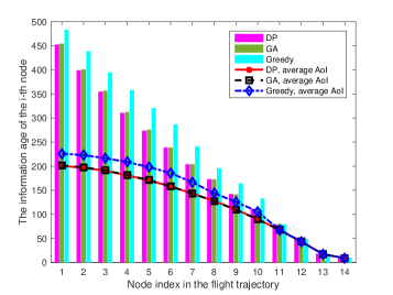
Figure 3: The minimum average AoI $\overline{X}_{i}^{*}$ in the Ave-AoI-optimal trajectory with $M=14$ SNs.

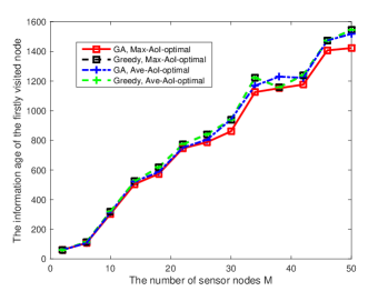
Figure 4: The minimum AoI $X_{1}^{*}$ versus the number of SNs $M$ in the Max-AoI-optimal and Ave-AoI-optimal trajectories.

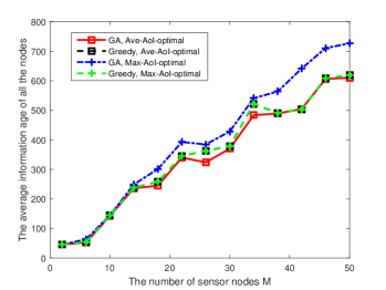
Figure 5: The minimum average AoI $\overline{X}_{1}^{*}$ versus the number of SNs $M$ in the Max-AoI-optimal and Ave-AoI-optimal trajectories.

V Simulation Results

In this section, we present simulation results to demonstrate the performance of the two trajectory planning algorithms. We consider a UAV-enabled wireless sensor network that consists of one data center, one UAV and $M$ SNs. The nodes are randomly located in a circular area of radius $1000$m. The UAV is dispatched to collect data from all the SNs exactly once along the flight trajectory. The flight height and velocity are set as $50$m and $20$m/s, respectively. The sensed data of each SN is uploaded to the UAV via a LOS link. The system bandwidth is equal to $B=5$ MHz, and the channel power gain at the reference distance $d_{0}=1$ m is set as $\beta=-60$ dB. The node’s transmission power and the noise power are set as $P_{i}=0.1$ watt and $\sigma^{2}=-110$ dBm, respectively. The data sensing time at each node is assumed to be very small and negligible. Suppose that the UAV takes off at time $T_{0}=0$.

In simulations, the Max-AoI-optimal and Ave-AoI-optimal trajectories are found using the three algorithms as follows: 1) the DP-based algorithm, i.e., Algorithm 1; 2) the GA-based algorithm, i.e., Algorithm 2; 3) the greedy algorithm that recursively finds the nearest predecessor $v_{(i-1)}$ for the node $v_{(i)}$ at each stage $i=M+1,M,\cdots,2$. More specifically, the node closest to the data center $v_{0}=v_{(M+1)}$ is selected and marked as node $v_{(M)}$. Similarly, among the unmarked nodes, the node nearest to node $v_{(i)}$ is selected as node $v_{(i-1)}$. This iterative procedure repeats until all the $M$ nodes constitute a Hamiltonian path. The GA related parameters are set as $N_{c}=10^{3}$, $N_{g}=10^{4}$, $\alpha=2$, $\gamma_{c}=0.8$ and $\gamma_{m}=0.01$.

In Fig. 2 and Fig. 3, we present the AoI $X_{i}^{*}$ of node $v_{(i)}$ in the Max-AoI-optimal and Ave-AoI-optimal trajectories, respectively. In this simulation, we consider a data collecting network with $M=14$. For comparison, we also plot the minimum average AoI $\overline{X}_{i}^{*}$ versus the node index $i$ in Fig. 3. From these figures, the information ages $X_{i}^{*}$ and $\overline{X}_{i}^{*}$ monotonically decreases with the node index $i$, in accordance with the results in Lemma 1 and Eq. (13). Among the three algorithms, the DP-based algorithm performs the best in terms of the AoI $X_{1}^{*}$ and $\overline{X}_{1}^{*}$, since it can find the Max-AoI-optimal and Ave-AoI-optimal trajectories by comparing all the candidate Hamiltonian paths. By intelligent search, the GA-based algorithm can find near optimal trajectories on which $X_{1}$ and $\overline{X}_{1}$ are very close to the minimum ones $X_{1}^{*}$ and $\overline{X}_{1}^{*}$. In contrast, the greedy algorithm achieves the largest AoIs $X_{1}$ and $\overline{X}_{1}$, since it just finds the local optimum at each stage.

The AoI $X_{i}^{*}$ of node $v_{(i)}$ ($i=2,\cdots,M$) found by the DP algorithm may not be the smallest, as shown in Fig. 2. In this figure, the ages of information $X_{i}^{*}$ for $i=4,\cdots,12$ calculated by the DP algorithm are larger than that by the GA algorithm. Similarly, $X_{i}^{*}$ for $i=10,\cdots,14$ are larger than that obtained by the greedy algorithm. This is because that any part of the globally optimal Hamiltonian path is not necessary to be locally optimal. Different from the Max-AoI-optimal trajectory planning case, the ages of information $X_{i}^{*}$ and $\overline{X}_{i}^{*}$ collected from the nodes in the Ave-AoI-optimal trajectory found by the GA and DP algorithms are very close, and are less than that obtained by the greedy algorithm, as shown in Fig. 3. This implies that the AoI metrics play the very important role in the flight trajectory planning.

In Fig. 4 and Fig. 5, we plot the minimum AoI of the firstly visited node $X_{1}^{*}$ and the minimum average AoI $\overline{X}_{1}^{*}$, respectively, when the Max-AoI-optimal and Ave-AoI-optimal trajectories are found by the GA and greedy algorithms. In Fig. 4, the information age $X_{1}^{*}$ in the Max-AoI-optimal trajectory is smaller than that in the Ave-AoI-optimal trajectory, when the GA algorithm is applied. Similarly, the Ave-AoI-optimal trajectory achieves a much smaller average AoI $\overline{X}_{1}^{*}$ than the Max-AoI-optimal trajectory. Again, this points out the importance of the AoI metric in the flight trajectory planning. When the greedy algorithm is applied, the Max-AoI-optimal and Ave-AoI-optimal trajectories are exactly the same, since the greedy algorithm always selects the the nearest neighbor among the candidate nodes at each stage in either the Max-AoI-optimal or Ave-AoI-optimal trajectory. It is also shown that the greedy algorithm performs better in finding the Ave-AoI-optimal trajectory than finding the Max-AoI-optimal trajectory, due to the increasing weight with the stage index.

VI Conclusions

This paper studied the Max-AoI-optimal and Ave-AoI-optimal trajectory planning problems for UAV-enabled data collection in wireless sensor networks. It was shown that the two age-optimal trajectories are exactly two shortest Hamiltonian paths in a weighted complete graph. Then, we developed DP and GA based algorithms to find Max-AoI-optimal and Ave-AoI-optimal trajectories in a unified way. By simulations, we showed that the proposed algorithms can find the age-optimal trajectories efficiently, compared to the baseline greedy algorithm. Based on the two AoI metrics, the UAV’s trajectory design helps to keep the sensed data fresh in wireless sensor networks.

References

- [1] N. H. Motlagh, T. Taleb, and O. Arouk, “Low-altitude unmanned aerial vehicles-based internet of things services: Comprehensive survey and future perspectives,” IEEE Internet of Things Journal, vol. 3, no. 6, pp. 899–922, Dec. 2016.
- [2] D. Yang, Q. Wu, Y. Zeng, and R. Zhang, “Energy trade-off in ground-to-UAV communication via trajectory design,” Sep. 2017. [Online]. Available: https://arxiv.org/pdf/1709.02975.pdf
- [3] A. E. A. A. Abdulla, Z. M. Fadlullah, H. Nishiyama, N. Kato, F. Ono, and R. Miura, “An optimal data collection technique for improved utility in UAS-aided networks,” in in Proc. IEEE Int. Conf. Comput. Commun. (INFOCOM), Toronto, Canada, May 2014, pp. 736–744.
- [4] S. Say, H. Inata, J. Liu, and S. Shimamoto, “Priority-based data gathering framework in UAV-assisted wireless sensor networks,” IEEE Sensors Journal, vol. 16, no. 14, pp. 5785–5794, Jul. 2016.
- [5] C. Zhan, Y. Zeng, and R. Zhang, “Energy-efficient data collection in UAV enabled wireless sensor network,” IEEE Wireless Commun. Letters, 2017. [Online]. Available: http://ieeexplore.ieee.org/stamp/stamp.jsp?tp=&arnumber=8119562
- [6] S. Kaul, R. Yates, and M. Gruteser, “Real-time status: How often should one update?” in Proc. INFOCOM, Orlando, FL, USA, Mar. 2012, pp. 2731–2735.
- [7] C. Kam, S. Kompella, and A. Ephremides, “Age of information under random updates,” in in Proc. IEEE ISIT, Jul. 2013, pp. 66–70.
- [8] Y. Sun, E. Uysal-Biyikoglu, R. Yates, C. E. Koksal, and N. B. Shroff, “Update or wait: How to keep your data fresh,” IEEE Trans. Inf. Theory, vol. 63, no. 11, pp. 7492–7508, Nov. 2017.
- [9] R. Diestel, Graph Theory, 5th ed. Springer-Verlag, Heidelberg, 2016.